CARNEGIE MELLON UNIVERSITY

DOCTORAL THESIS

Algorithms for Ranking and RoutingProblems

Author:Yang JIAO

Supervisor:R. RAVI

Dissertation Committee:R. Ravi (Chair)

Gérard CornuéjolsWillem-Jan van Hoeve

Ojas ParekhCynthia Phillips

A thesis submitted in fulfillment of the requirementsfor the degree of Doctor of Philosophy

in the

Algorithms, Combinatorics, and OptimizationTepper School of Business, Carnegie Mellon University

September 7, 2018

iii

Declaration of AuthorshipI, Yang JIAO, declare that this thesis titled, “Algorithms for Ranking and RoutingProblems” and the work presented in it are my own. I confirm that:

• This work was done wholly or mainly while in candidature for a research de-gree at this University.

• Where any part of this thesis has previously been submitted for a degree orany other qualification at this University or any other institution, this has beenclearly stated.

• Where I have consulted the published work of others, this is always clearlyattributed.

• Where I have quoted from the work of others, the source is always given. Withthe exception of such quotations, this thesis is entirely my own work.

• I have acknowledged all main sources of help.

• Where the thesis is based on work done by myself jointly with others, I havemade clear exactly what was done by others and what I have contributed my-self.

Signed:

Date:

v

CARNEGIE MELLON UNIVERSITY

AbstractTepper School of Business, Carnegie Mellon University

Doctor of Philosophy

Algorithms for Ranking and Routing Problems

by Yang JIAO

In this thesis, we develop new algorithms for two categories of problems–rankingand routing. In the first category, we classify the complexity of new problems formutually ranking participants and tasks when a ranking of the participants “nearby"the optimal is given. In the second category, we give approximation algorithmsfor inventory routing on line metrics, two new variants of inventory routing, andprovide fast heuristics for inventory routing on arbitrary metrics.

For the first category, we introduce and resolve the computational complexity ofa set of new problems that require ranking participants and tasks by their strengthsand difficulties, respectively, given the set of tasks that each participant completedsuccessfully. The ideal ranking ensures that stronger participants succeed at all tasksthat weaker participants performed successfully and easier tasks are performed suc-cessfully by all the participants who succeeded at harder tasks. The new variantswe introduce and study account for recurring participants, by constraining the out-come of the current ranking to be close to an initial given ranking of the participantsarrived from past contests. We provide a comprehensive study of the complexity ofall the variants.

The second category involves three sets of routing problems. The first amongthem is the Inventory Routing Problem (IRP). Given clients on a metric, each withdaily demands that must be delivered from a depot, and holding costs over the plan-ning horizon, a solution selects a set of daily routes from the depot through a subsetof clients to deliver all demands before they are due. The cost of the solution com-bines the costs of the routes with the holding cost of the demand that arrives earlierat clients. For Inventory Routing on line metrics, we give a constant approximationalgorithms by LP rounding and a primal dual method. We also study the computa-tional aspect of IRP on general metrics. We design fast combinatorial heuristics forIRP by connecting them to prize-collecting vehicle routing problems and evaluatetheir performance on randomly generated data sets. The second variant of IRP westudy is called Deadline IRP. In this version, every client has a deadline within whichit will run out if it starts at full capacity, and each visit to every client fills the clientlocation to capacity. The goal is to determine an IRP solution so that no client everruns out. We provide logarithmic approximations and show a class of instances forwhich our method cannot improve the approximation factor. The third set of routingproblems we study are variants of Inventory Routing with Facility Location, whichallows multiple depot locations to be opened for service at an extra cost. We providea 12-approximation for Star Inventory Routing with Facility Location assuming thatclients connect directly to the opened facilities.

vii

AcknowledgementsFirst, I am deeply grateful to my advisor R. Ravi, whose continuous enthusiasm

has been an inspiration to me for the past five years. I am indebted to the generoustime and effort he has spent developing my research skills and communication skills.His sharp intuition for a wide range of problems has helped me develop better waysto visualize and solve new problems. I also appreciate Ravi’s approachability andwillingness to meet beyond our regularly scheduled hours whenever I needed. Hisabundant and prompt feedback on my many drafts and talks has significantly im-proved my ability to communicate technical ideas clearly. Ravi has encouraged andsupported me to attend workshops/conferences and present my research at everyopportunity. I cannot thank him enough for all he has done for my development.

Additionally, I would like to thank Ojas Parekh for hosting me at Sandia andintroducing me to the emerging field of quantum computing. Ojas’s excitement forquantum computing has positively influenced me to keep an eye out for new areasrelated to my research. I also appreciate him kindly taking me to the many hospitalvisits during the occurrence of my health problems at Sandia. During my internshipwith Ojas, I was fortunate to have the opportunity to have met Cindy Phillips. Iwould like to thank her for her professional advice and for inviting me to presentmy work at SIAM.

During my work on the ranking related problems, I had the opportunity to col-laborate with Wolfgang Gatterbauer. I would like to thank him for the discussionsand the detailed feedback he gave on my paper and presentation.

Also, I would like to thank all of my committee members, R. Ravi, Gérard Cor-nuéjols, Willem-Jan van Hoeve, Ojas Parekh, and Cindy Phillips, for providing valu-able feedback on my drafts and talks.

Before I first came into the field, I had an excellent teacher, Rajiv Gandhi, whokindled my love for algorithms. I thank him for believing in the best of all his stu-dents and for inspiring me to delve deeper into theoretical computer science.

I extend my thanks to Lawrence Rapp and Laila Lee, who helped the PhD processrun smoothly.

Finally, I would like to thank my family, friends, and peers for keeping me mo-tivated to the end. In particular, thanks to Anuj, Arash, Christian, Dabeen, Eric,Gerdus, Jenny, Ji, John, Nam, Ryo, Sagnik, Shirley, Stelios, Thiago, Thomas, andWenting for their helpful discussions and friendship. I thank my parents for theirunwavering love and support throughout my life.

ix

Contents

Declaration of Authorship iii

Abstract v

Acknowledgements vii

1 Introduction 1

2 Algorithms for Automatic Ranking of Participants and Tasks in an AnonymizedContest 52.1 Introduction . . . . . . . . . . . . . . . . . . . . . . . . . . . . . . . . . . 5

2.1.1 Motivation . . . . . . . . . . . . . . . . . . . . . . . . . . . . . . . 52.1.2 Problem Formulations . . . . . . . . . . . . . . . . . . . . . . . . 72.1.3 Basic Variants of Chain Editing . . . . . . . . . . . . . . . . . . . 72.1.4 Main Results . . . . . . . . . . . . . . . . . . . . . . . . . . . . . 10

2.2 Related Work . . . . . . . . . . . . . . . . . . . . . . . . . . . . . . . . . 122.3 Polynomial Time Algorithms for k-near Orderings . . . . . . . . . . . . 13

2.3.1 Constrained k-near . . . . . . . . . . . . . . . . . . . . . . . . . . 132.3.2 Unconstrained k-near . . . . . . . . . . . . . . . . . . . . . . . . 162.3.3 Both k-near . . . . . . . . . . . . . . . . . . . . . . . . . . . . . . 19

2.4 Conclusion . . . . . . . . . . . . . . . . . . . . . . . . . . . . . . . . . . . 21

3 Inventory Routing on Line Metrics 233.1 Introduction . . . . . . . . . . . . . . . . . . . . . . . . . . . . . . . . . . 233.2 Related Work . . . . . . . . . . . . . . . . . . . . . . . . . . . . . . . . . 243.3 Primal Rounding for Line . . . . . . . . . . . . . . . . . . . . . . . . . . 253.4 Primal Dual . . . . . . . . . . . . . . . . . . . . . . . . . . . . . . . . . . 27

3.4.1 LP Formulation . . . . . . . . . . . . . . . . . . . . . . . . . . . . 273.4.2 Basic Primal Dual Phase and Analysis . . . . . . . . . . . . . . . 283.4.3 Example with High Routing Cost . . . . . . . . . . . . . . . . . 313.4.4 Pruning Phase and Analysis . . . . . . . . . . . . . . . . . . . . . 32

3.5 Open Questions . . . . . . . . . . . . . . . . . . . . . . . . . . . . . . . . 35

4 Combinatorial Heuristics for Inventory Routing on General Metrics 374.1 Introduction . . . . . . . . . . . . . . . . . . . . . . . . . . . . . . . . . . 374.2 Related Work . . . . . . . . . . . . . . . . . . . . . . . . . . . . . . . . . 404.3 Local Search . . . . . . . . . . . . . . . . . . . . . . . . . . . . . . . . . . 41

4.3.1 DELETE . . . . . . . . . . . . . . . . . . . . . . . . . . . . . . . . 424.3.2 ADD . . . . . . . . . . . . . . . . . . . . . . . . . . . . . . . . . . 424.3.3 Prioritized Local Search . . . . . . . . . . . . . . . . . . . . . . . 44

4.4 Greedy Heuristic . . . . . . . . . . . . . . . . . . . . . . . . . . . . . . . 454.4.1 Greedy Framework . . . . . . . . . . . . . . . . . . . . . . . . . . 454.4.2 Approximate Minimum Density Set . . . . . . . . . . . . . . . . 46

x

4.4.3 Implementation Detail . . . . . . . . . . . . . . . . . . . . . . . . 484.5 Primal Dual . . . . . . . . . . . . . . . . . . . . . . . . . . . . . . . . . . 49

4.5.1 LP Formulation . . . . . . . . . . . . . . . . . . . . . . . . . . . . 494.5.2 A Primal-dual Approach . . . . . . . . . . . . . . . . . . . . . . 504.5.3 Defining a Feasible Dual . . . . . . . . . . . . . . . . . . . . . . . 534.5.4 Implementation . . . . . . . . . . . . . . . . . . . . . . . . . . . . 54

4.6 Benchmark MIP Formulation . . . . . . . . . . . . . . . . . . . . . . . . 544.7 Computational Results . . . . . . . . . . . . . . . . . . . . . . . . . . . . 56

4.7.1 Data Generation Model . . . . . . . . . . . . . . . . . . . . . . . 584.7.2 Performance Evaluation . . . . . . . . . . . . . . . . . . . . . . . 584.7.3 Conclusions . . . . . . . . . . . . . . . . . . . . . . . . . . . . . . 63

4.8 Acknowledgments . . . . . . . . . . . . . . . . . . . . . . . . . . . . . . 65

5 Deadline Inventory Routing Problem 675.1 Introduction . . . . . . . . . . . . . . . . . . . . . . . . . . . . . . . . . . 675.2 Related Work . . . . . . . . . . . . . . . . . . . . . . . . . . . . . . . . . 685.3 Approximation Algorithms . . . . . . . . . . . . . . . . . . . . . . . . . 695.4 Conclusion . . . . . . . . . . . . . . . . . . . . . . . . . . . . . . . . . . . 74

6 Inventory Routing Problem with Facility Location 756.1 Related Work . . . . . . . . . . . . . . . . . . . . . . . . . . . . . . . . . 756.2 Inventory Access Problem . . . . . . . . . . . . . . . . . . . . . . . . . . 76

6.2.1 Uncapacitated IAP . . . . . . . . . . . . . . . . . . . . . . . . . . 766.2.2 Capacitated Unsplittable IAP . . . . . . . . . . . . . . . . . . . . 766.2.3 Capacitated Splittable IAP . . . . . . . . . . . . . . . . . . . . . . 77

6.3 Uncapacitated SIRPFL . . . . . . . . . . . . . . . . . . . . . . . . . . . . 796.4 Conclusion . . . . . . . . . . . . . . . . . . . . . . . . . . . . . . . . . . . 83

7 Conclusion 85

Bibliography 87

xi

List of Figures

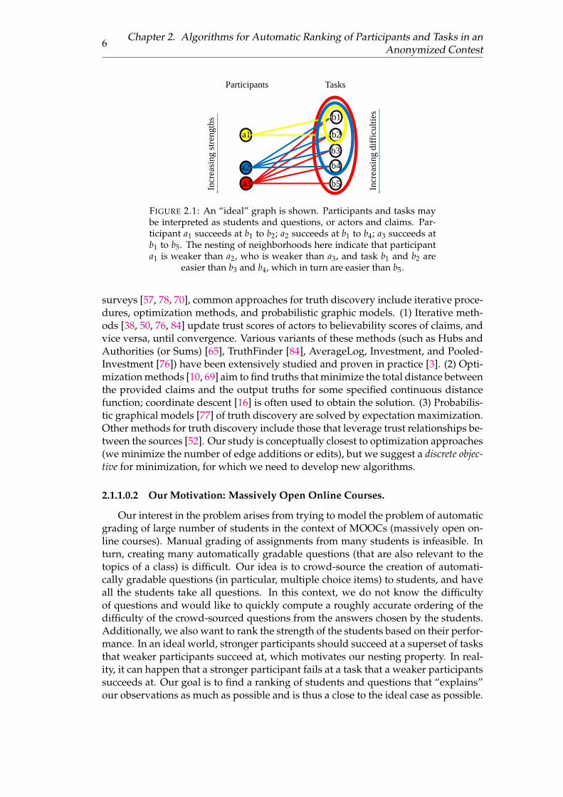
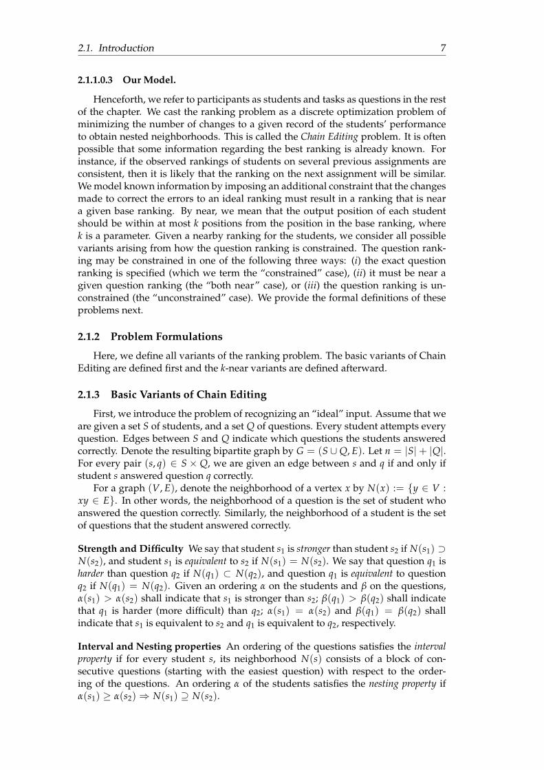
2.1 An “ideal” graph is shown. Participants and tasks may be interpretedas students and questions, or actors and claims. Participant a1 suc-ceeds at b1 to b2; a2 succeeds at b1 to b4; a3 succeeds at b1 to b5. Thenesting of neighborhoods here indicate that participant a1 is weakerthan a2, who is weaker than a3, and task b1 and b2 are easier than b3and b4, which in turn are easier than b5. . . . . . . . . . . . . . . . . . . 6

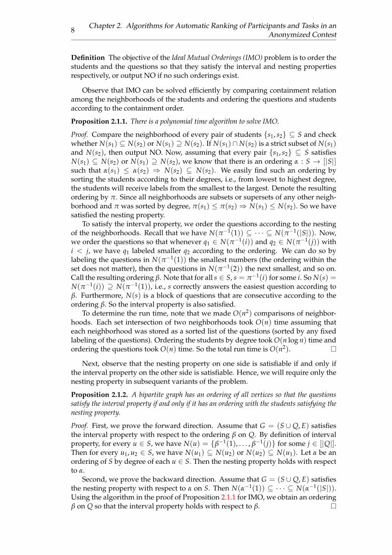
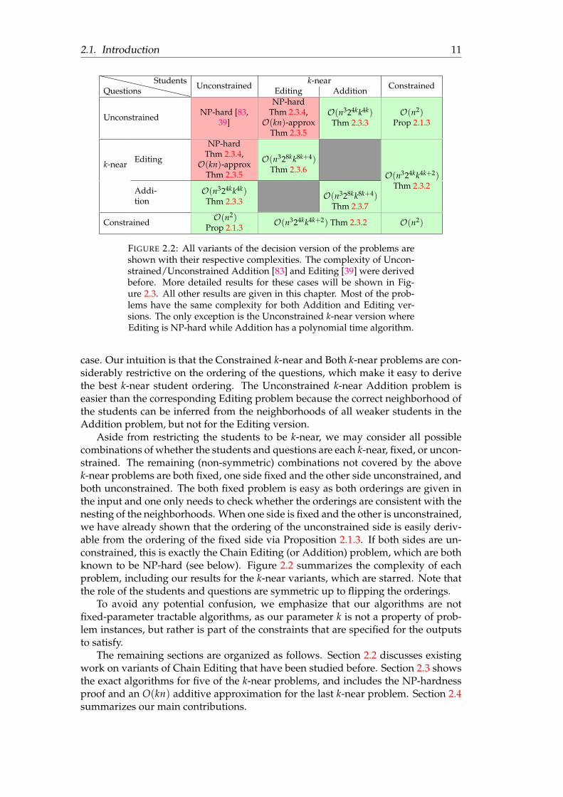
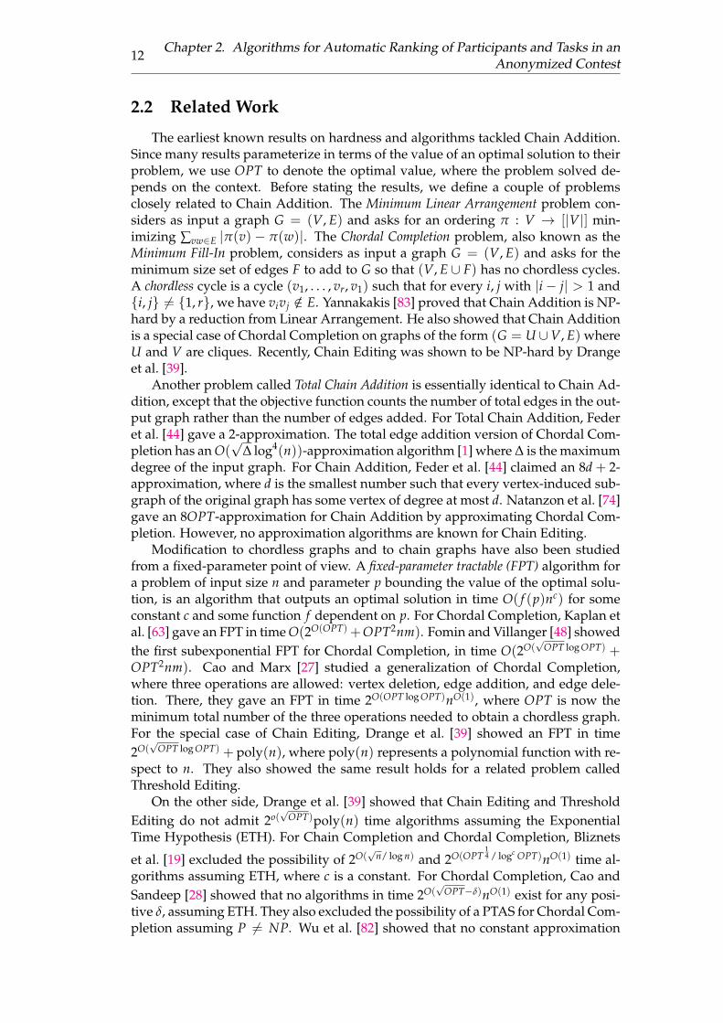
2.2 All variants of the decision version of the problems are shown withtheir respective complexities. The complexity of Unconstrained/UnconstrainedAddition [83] and Editing [39] were derived before. More detailed re-sults for these cases will be shown in Figure 2.3. All other results aregiven in this chapter. Most of the problems have the same complexityfor both Addition and Editing versions. The only exception is the Un-constrained k-near version where Editing is NP-hard while Additionhas a polynomial time algorithm. . . . . . . . . . . . . . . . . . . . . . . 11

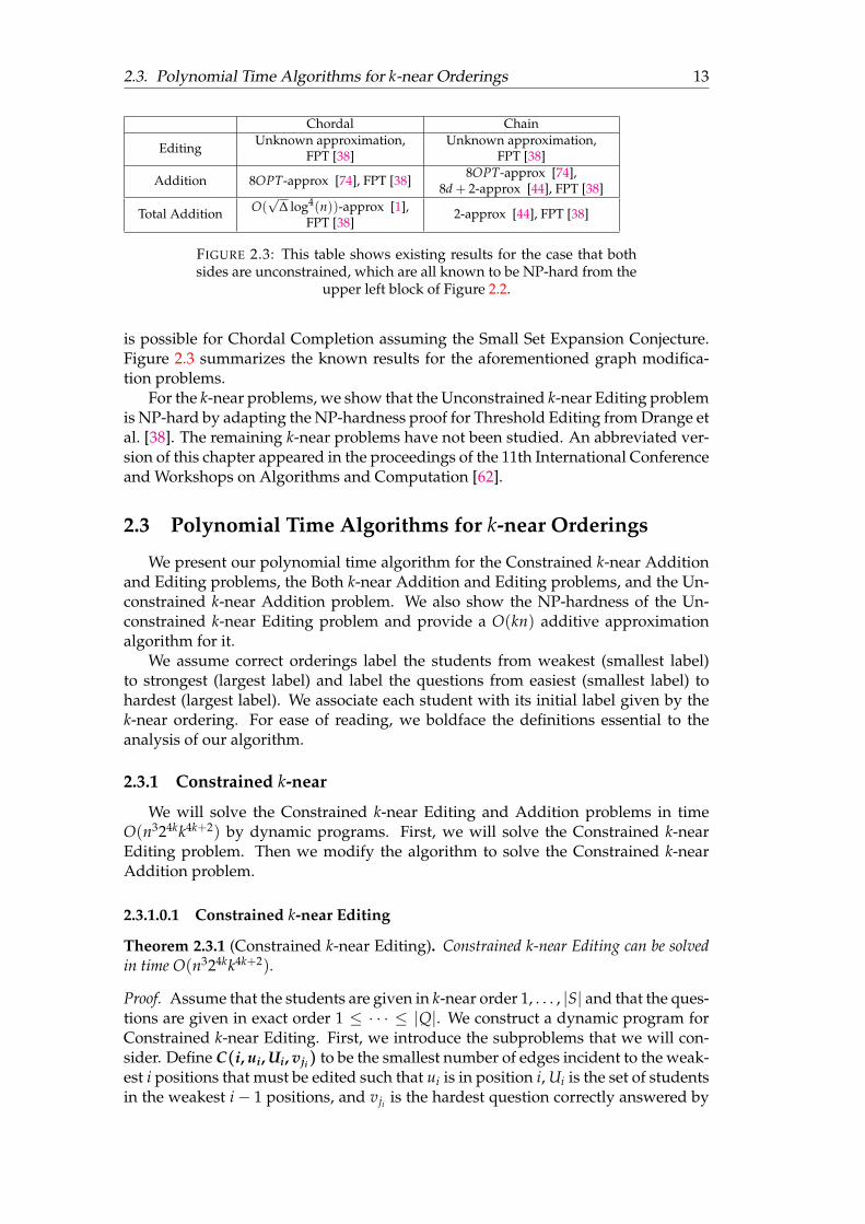
2.3 This table shows existing results for the case that both sides are un-constrained, which are all known to be NP-hard from the upper leftblock of Figure 2.2. . . . . . . . . . . . . . . . . . . . . . . . . . . . . . . 13

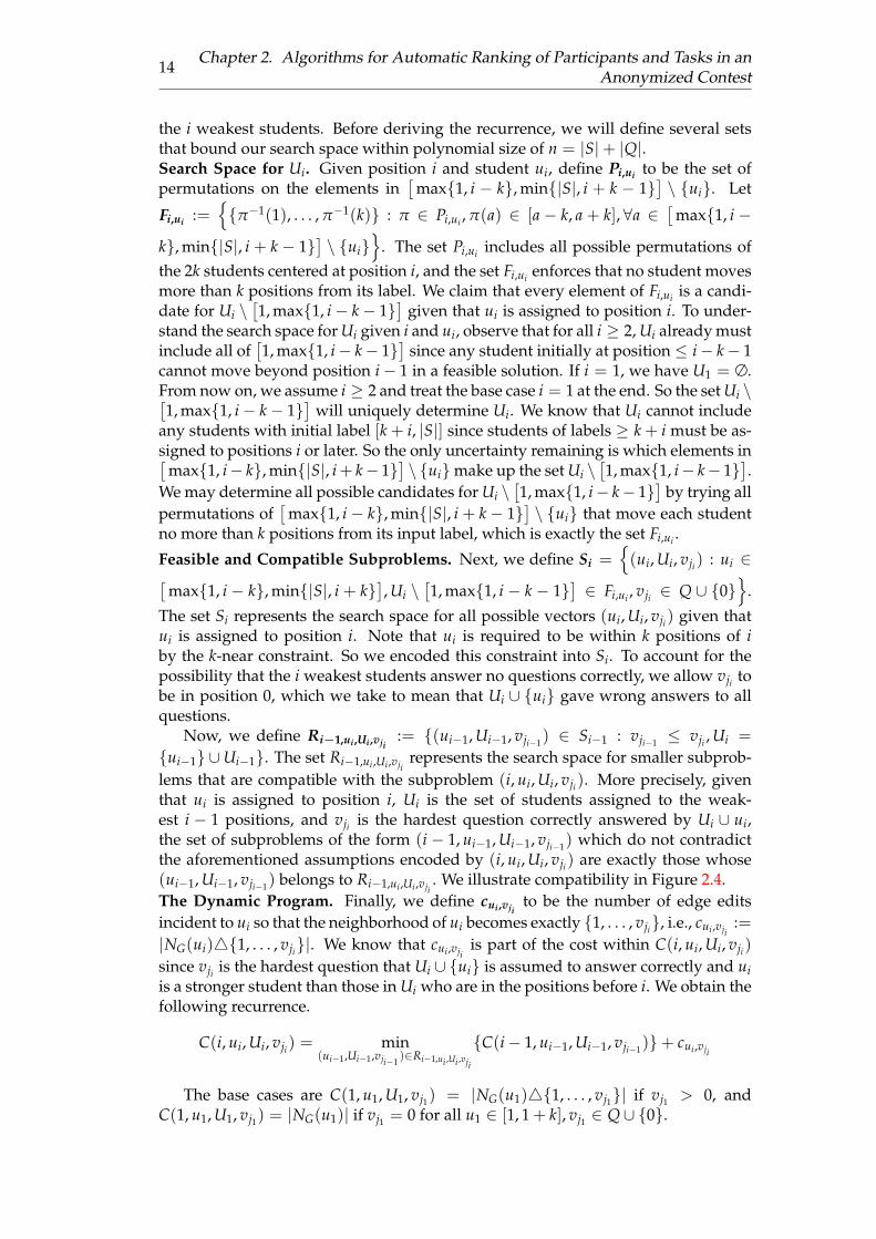
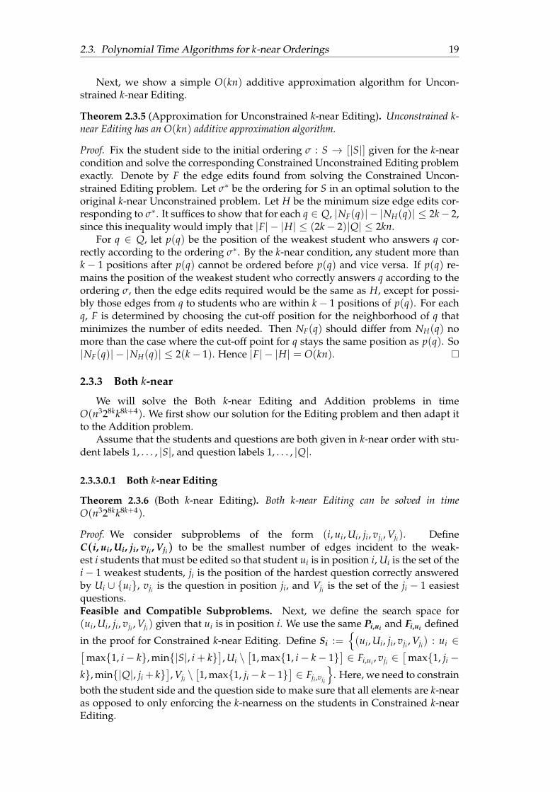
2.4 Subproblem (i− 1, ui−1, Ui−1, vji−1) is compatible with subproblem (i, ui, Ui, vji)if and only if vji−1 is no harder than vji and Ui = ui−1 ∪Ui−1. Thecost of (i, ui, Ui, vji) is the sum of the minimum cost among feasi-ble compatible subproblems of the form (i − 1, ui−1, Ui−1, vji−1) andthe number of edits incident to ui to make its neighborhood exactly1, . . . , vji. . . . . . . . . . . . . . . . . . . . . . . . . . . . . . . . . . . . 15

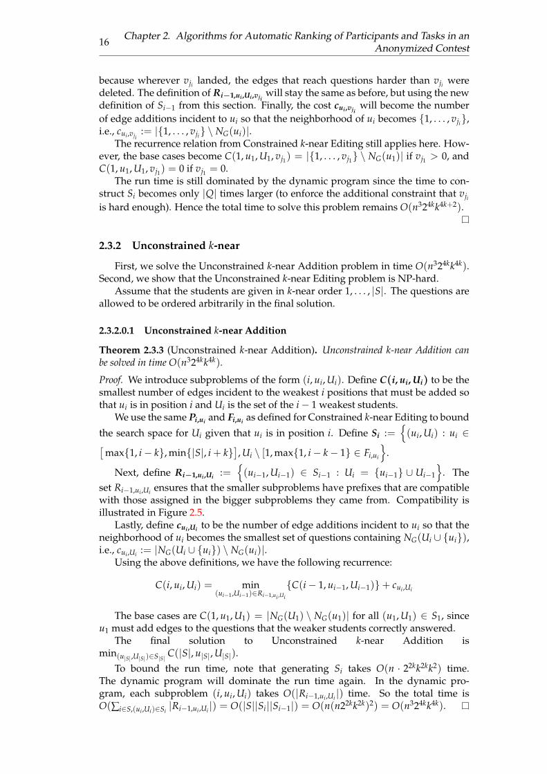
2.5 Subproblem (i− 1, ui−1, Ui−1) is compatible with subproblem (i, ui, Ui)if and only if Ui = ui−1 ∪Ui−1. The cost of (i, ui, Ui) is sum of theminimum cost among feasible compatible subproblems of the form(i− 1, ui−1, Ui−1) and the number of additions incident to ui to makeits neighborhood the smallest set of questions containing the existingneighbors of Ui. . . . . . . . . . . . . . . . . . . . . . . . . . . . . . . . . 17

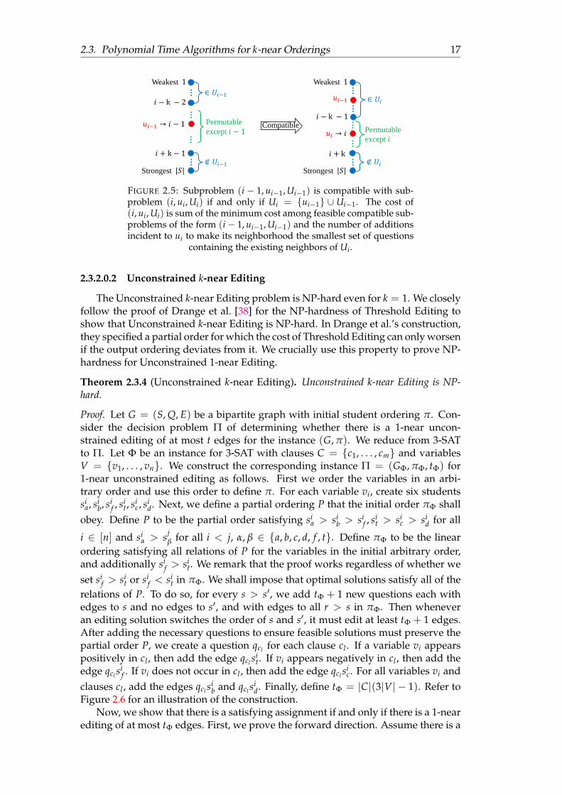
2.6 Each set of six vertices represents the students corresponding to avariable x, y, or z. The bottom vertex represents a question corre-sponding to the clause cl = w ∨ x ∨ y. . . . . . . . . . . . . . . . . . . . 18

2.7 Subproblem (i − 1, ui−1, Ui−1, ji−1, vji−1 , Vji−1) is compatible with sub-problem (i, ui, Ui, ji, vji , Vji) if and only if Ui = ui ∪Ui−1, ji−1 rep-resents a position no harder than ji, Vji ∪ vji contains Vji−1 ∪ vji−1,and ji−1 strictly easier than ji implies that Vji contains Vji−1 ∪ vji−1.The cost of (i, ui, Ui, ji, vji , Vji) is the sum of the minimum cost amongfeasible compatible states of the form (i− 1, ui−1, Ui−1, ji−1, vji−1 , Vji−1)and the number of edits incident to ui that makes its neighborhoodVji ∪ vji. . . . . . . . . . . . . . . . . . . . . . . . . . . . . . . . . . . . 20

xii

3.1 Each arrow from an edge to a location indicates that accumulation ofthe LP values of that edge determines the times assigned to visits upto that location. . . . . . . . . . . . . . . . . . . . . . . . . . . . . . . . . 26

3.2 The red dots at location Di time s indicate that visit s is the freezingvisit of the demand point (i, t) whose [ f reeze(i, t), t] 3 s. The horizon-tal colored portion of each active interval [ f reeze(i, t), t] represents theamount βi

s,t = Hif reeze(i,t),t − Hi

s,t that (i, t) contributes to the routingcost of visit s of the same color. . . . . . . . . . . . . . . . . . . . . . . . 30

3.3 The above shows the active intervals of the instance in Example 1. . . . 323.4 βs′(i,t) ≥ Di(i,t)

/2. . . . . . . . . . . . . . . . . . . . . . . . . . . . . . . . . 34

3.5 At most one freezing visit charges bit per Fk. . . . . . . . . . . . . . . . . 35

3.6 At most three freezing visits total charge bit. . . . . . . . . . . . . . . . . 36

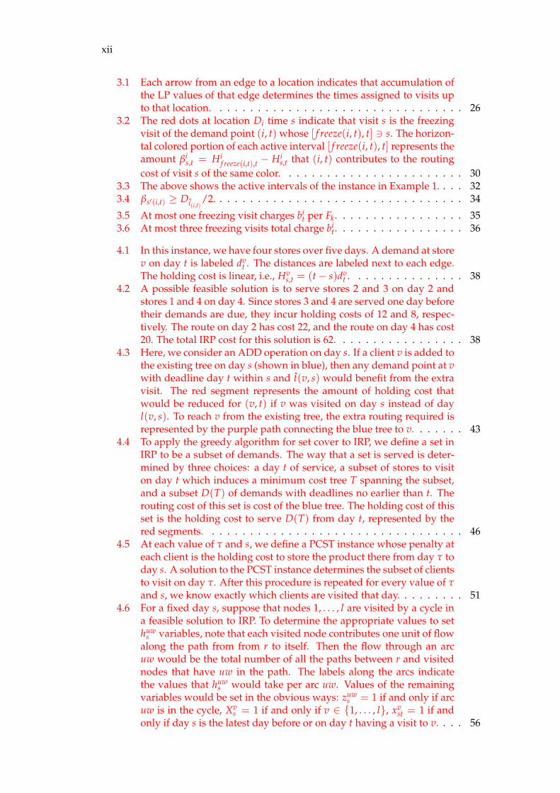
4.1 In this instance, we have four stores over five days. A demand at storev on day t is labeled dv

t . The distances are labeled next to each edge.The holding cost is linear, i.e., Hv

s,t = (t− s)dvt . . . . . . . . . . . . . . . 38

4.2 A possible feasible solution is to serve stores 2 and 3 on day 2 andstores 1 and 4 on day 4. Since stores 3 and 4 are served one day beforetheir demands are due, they incur holding costs of 12 and 8, respec-tively. The route on day 2 has cost 22, and the route on day 4 has cost20. The total IRP cost for this solution is 62. . . . . . . . . . . . . . . . . 38

4.3 Here, we consider an ADD operation on day s. If a client v is added tothe existing tree on day s (shown in blue), then any demand point at vwith deadline day t within s and t(v, s) would benefit from the extravisit. The red segment represents the amount of holding cost thatwould be reduced for (v, t) if v was visited on day s instead of dayl(v, s). To reach v from the existing tree, the extra routing required isrepresented by the purple path connecting the blue tree to v. . . . . . . 43

4.4 To apply the greedy algorithm for set cover to IRP, we define a set inIRP to be a subset of demands. The way that a set is served is deter-mined by three choices: a day t of service, a subset of stores to visiton day t which induces a minimum cost tree T spanning the subset,and a subset D(T) of demands with deadlines no earlier than t. Therouting cost of this set is cost of the blue tree. The holding cost of thisset is the holding cost to serve D(T) from day t, represented by thered segments. . . . . . . . . . . . . . . . . . . . . . . . . . . . . . . . . . 46

4.5 At each value of τ and s, we define a PCST instance whose penalty ateach client is the holding cost to store the product there from day τ today s. A solution to the PCST instance determines the subset of clientsto visit on day τ. After this procedure is repeated for every value of τand s, we know exactly which clients are visited that day. . . . . . . . . 51

4.6 For a fixed day s, suppose that nodes 1, . . . , l are visited by a cycle ina feasible solution to IRP. To determine the appropriate values to sethuw

s variables, note that each visited node contributes one unit of flowalong the path from from r to itself. Then the flow through an arcuw would be the total number of all the paths between r and visitednodes that have uw in the path. The labels along the arcs indicatethe values that huw

s would take per arc uw. Values of the remainingvariables would be set in the obvious ways: zuw

s = 1 if and only if arcuw is in the cycle, Xv

s = 1 if and only if v ∈ 1, . . . , l, xvst = 1 if and

only if day s is the latest day before or on day t having a visit to v. . . . 56

xiii

4.7 Delete, Add, and Prioritized each correspond to the local search thatDELETEs, ADDs, and all operations, respectively. The gaps and run-ning times for Delete, Add, Prioritized local search, Greedy, PrunedGreedy, Primal Dual, and Pruned Primal Dual are shown in blue, red,green, purple, light blue, orange, and dark blue, respectively. . . . . . . 60

4.8 The gaps and running times for Delete, Add, Prioritized local search,Greedy, Pruned Greedy, Primal Dual, and Pruned Primal Dual areshown in blue, red, green, purple, light blue, orange, and dark blue,respectively. . . . . . . . . . . . . . . . . . . . . . . . . . . . . . . . . . . 62

4.9 The gaps and running times for Delete, Add, Prioritized local search,Greedy, Pruned Greedy, Primal Dual, and Pruned Primal Dual areshown in blue, red, green, purple, light blue, orange, and dark blue,respectively. . . . . . . . . . . . . . . . . . . . . . . . . . . . . . . . . . . 64

5.1 Illustration of G2, (depletion times in circles) . . . . . . . . . . . . . . . 725.2 Illustration of H2 . . . . . . . . . . . . . . . . . . . . . . . . . . . . . . . 72

xv

Dedicated to my parents

1

Chapter 1

Introduction

MotivationWe study a set of ranking problems and three types of routing problems that

involve coordinating schedules with the routes. The ranking problems arise fromthe context of Massive Open Online Courses, where the large number of studentsmake it challenging to create appropriate ways to evaluate students such that theirresults can all be graded efficiently for timely feedback. One way to speed up theprocess is to restrict the test questions to automatically gradable questions e.g. mul-tiple choice. Furthermore, to quickly create a large number of test questions, weconsider crowd-sourcing the creation of test questions to the students. However,giving role of question creation to the students means that the instructor no longerknows the difficulty of the questions. So we would like to find ways to quickly rankthe difficulty of the newly created questions as well as the strength of the studentsafter they attempt all the questions. Chapter 2 models variants of the this rankingproblem and resolves their complexity.

Routing problems with scheduling components have been studied extensivelyon the computational side, but are fairly new within the theoretical realm. Althougha rich history of theoretical methods exist for network design problems (the routingcomponent), the integration of routing with scheduling create an interesting chal-lenge to obtaining theoretical guarantees. We study variants of a popular inventoryrouting problem in this thesis [80]. We consider the deterministic inventory routingproblem over a discrete finite time horizon. Given clients on a metric, each withdaily demands that must be delivered from a depot and holding costs over the plan-ning horizon, an optimal solution selects a set of daily tours through a subset ofclients to deliver all demands before they are due and minimizes the total holdingand tour routing costs over the horizon. In particular, the best approximation forInventory Routing Problem (on general metrics) has yet to break a logarithmic fac-tor. It is also unknown whether this problem can be shown to have a super constanthardness of approximation. Constant factor guarantees have only been shown forspecial cases such as when the metric is a tree or when the schedule is restricted tobe periodic. In the subsequent chapters, we extend LP-based methods to variantsof Inventory Routing and give fast heuristics that obtain near optimal solutions onrandomly generated data sets.SummaryRanking Problems The first category of problems we study are the ranking prob-lems of Chapter 2. Here, we introduce a new set of problems based on the ChainEditing problem. In our version of Chain Editing, we are given a set of participantsand a set of tasks that every participant attempts. For each participant-task pair,we know whether the participant has succeeded at the task or not. We assume thatparticipants vary in their ability to solve tasks, and that tasks vary in their difficultyto be solved. In an ideal world, stronger participants should succeed at a superset

2 Chapter 1. Introduction

of tasks that weaker participants succeed at. Similarly, easier tasks should be com-pleted successfully by a superset of participants who succeed at harder tasks. Inreality, it can happen that a stronger participant fails at a task that a weaker partici-pants succeeds at. Our goal is to find a perfect nesting of the participant-task relations byflipping a minimum number of participant-task relations, implying such a “nearestperfect ordering” to be the one that is closest to the truth of participant strengths andtask difficulties. Many variants of the problem are known to be NP-hard.

We propose six natural k-near versions of the Chain Editing problem and classifytheir complexity. The input to a k-near Chain Editing problem includes an initialordering of the participants (or tasks) that the final solution is required to be “close”to, by moving each participant (or task) at most k positions from the initial ordering.We obtain surprising results on the complexity of the six k-near problems: Five ofthe problems are polynomial-time solvable using dynamic programming, but one ofthem is NP-hard.Inventory Routing Problem The second category of problems consists of three typesof routing problems. The first among them is inventory routing, introduced in Chap-ter 3. For the special case that the metric is a line, we obtain a 5-approximation usingLP rounding and a 26-approximation using a primal dual algorithm.

Besides theoretical guarantees for the special case on line metrics, we study thecomputational side of IRP arbitrary metrics in Chapter 4. In particular, we providefast heuristics for IRP on general metrics that uses a Prize-Collecting Steiner Treesubproblem to guide the inventory routing solution to near optimality. Our bestheuristic solves instances of at least 160 clients over 6 days and 50 clients over 18days to near optimality in a few seconds. It is three orders of magnitude faster thansolving the single commodity flow MIP formulation using Gurobi cut off at 10%MIPGap.Deadline Inventory Routing Problem The second type of routing problem, intro-duced in Chapter 5, is called Deadline Inventory Routing, motivated by the replen-ishment of ATMs. In Deadline Inventory Routing, every client has a deadline withinwhich it will run out if it starts at full capacity, and each visit to every client fillsthe client location to capacity. The goal is to determine a set of routes, one for eachday, such that no client ever runs out. We show a log(n)-approximation, where nis the number of clients. To obtain the logarithmic approximation, we first reducefrom arbitrary instances to a subclass of instances where each deadline is a powerof 2 by losing a constant factor in the cost of the solution. Within powers-of-2 in-stances, a natural (though possibly costly) solution is one that visits on day l exactlythose clients whose deadlines 2i divide l (i.e., l is a multiple of 2i). We call sucha solution synchronized since it tries to group together as many clients as possiblewho are appropriate to visit per day. Next, we introduce nondecreasing solutions,which are those whose route per day must visit clients in nondecreasing order oftheir deadline values. We show that nondecreasing solutions have cost at most alogarithmic factor away from the cost of any arbitrary solution. Then, we show thatsynchronized solutions are derivable from nondecreasing solutions preserving theexact cost. So optimal synchronized solutions are also logarithmic factor from arbi-trary solutions. Since the set of clients to visit per day is completely determined insynchronized solutions, optimal synchronized solutions are easy to approximate byapproximating Steiner trees. Hence we obtain an O(log n)-approximation for Sta-tionary Deadline Inventory Routing. We show that the analysis for this method istight on an infinite class of instances. Using an LP-based approach, we also obtain alog(T)-approximation, where T is the number of days in the time horizon.

Chapter 1. Introduction 3

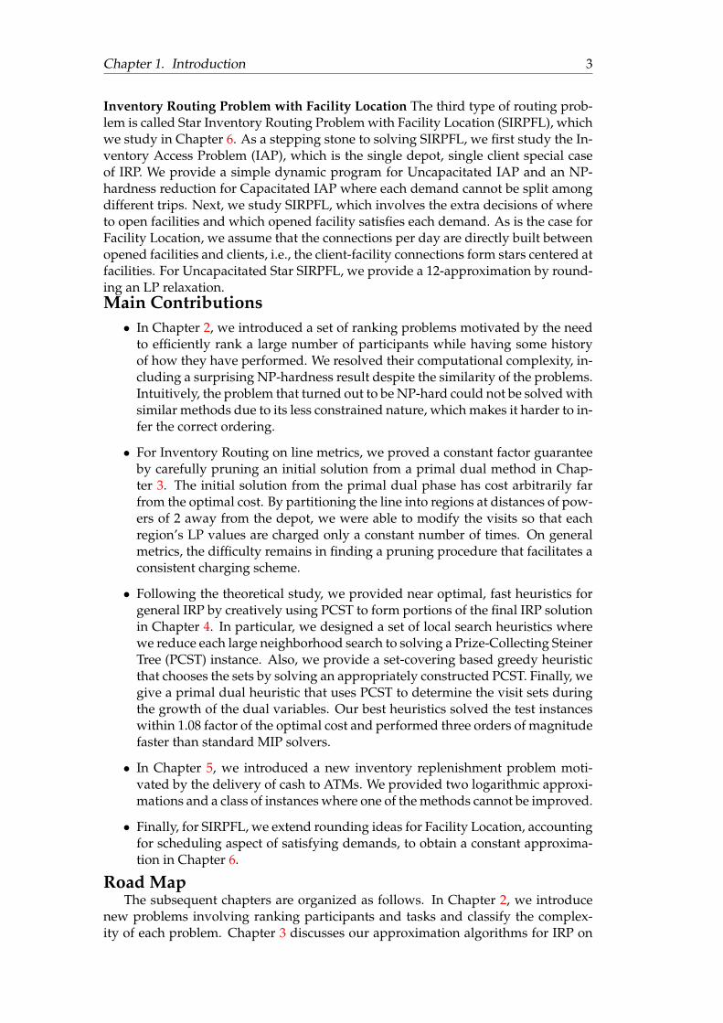
Inventory Routing Problem with Facility Location The third type of routing prob-lem is called Star Inventory Routing Problem with Facility Location (SIRPFL), whichwe study in Chapter 6. As a stepping stone to solving SIRPFL, we first study the In-ventory Access Problem (IAP), which is the single depot, single client special caseof IRP. We provide a simple dynamic program for Uncapacitated IAP and an NP-hardness reduction for Capacitated IAP where each demand cannot be split amongdifferent trips. Next, we study SIRPFL, which involves the extra decisions of whereto open facilities and which opened facility satisfies each demand. As is the case forFacility Location, we assume that the connections per day are directly built betweenopened facilities and clients, i.e., the client-facility connections form stars centered atfacilities. For Uncapacitated Star SIRPFL, we provide a 12-approximation by round-ing an LP relaxation.Main Contributions• In Chapter 2, we introduced a set of ranking problems motivated by the need

to efficiently rank a large number of participants while having some historyof how they have performed. We resolved their computational complexity, in-cluding a surprising NP-hardness result despite the similarity of the problems.Intuitively, the problem that turned out to be NP-hard could not be solved withsimilar methods due to its less constrained nature, which makes it harder to in-fer the correct ordering.

• For Inventory Routing on line metrics, we proved a constant factor guaranteeby carefully pruning an initial solution from a primal dual method in Chap-ter 3. The initial solution from the primal dual phase has cost arbitrarily farfrom the optimal cost. By partitioning the line into regions at distances of pow-ers of 2 away from the depot, we were able to modify the visits so that eachregion’s LP values are charged only a constant number of times. On generalmetrics, the difficulty remains in finding a pruning procedure that facilitates aconsistent charging scheme.

• Following the theoretical study, we provided near optimal, fast heuristics forgeneral IRP by creatively using PCST to form portions of the final IRP solutionin Chapter 4. In particular, we designed a set of local search heuristics wherewe reduce each large neighborhood search to solving a Prize-Collecting SteinerTree (PCST) instance. Also, we provide a set-covering based greedy heuristicthat chooses the sets by solving an appropriately constructed PCST. Finally, wegive a primal dual heuristic that uses PCST to determine the visit sets duringthe growth of the dual variables. Our best heuristics solved the test instanceswithin 1.08 factor of the optimal cost and performed three orders of magnitudefaster than standard MIP solvers.

• In Chapter 5, we introduced a new inventory replenishment problem moti-vated by the delivery of cash to ATMs. We provided two logarithmic approxi-mations and a class of instances where one of the methods cannot be improved.

• Finally, for SIRPFL, we extend rounding ideas for Facility Location, accountingfor scheduling aspect of satisfying demands, to obtain a constant approxima-tion in Chapter 6.

Road MapThe subsequent chapters are organized as follows. In Chapter 2, we introduce

new problems involving ranking participants and tasks and classify the complex-ity of each problem. Chapter 3 discusses our approximation algorithms for IRP on

4 Chapter 1. Introduction

line metrics. In Chapter 4, we give three combinatorial heuristics that utilize Prize-Collecting Steiner Tree solutions to find fast near optimal solutions for IRP. In Chap-ter 5, we propose a new variant of IRP called Deadline IRP and state our approaches.Chapter 6 introduces another variant of IRP, Star IRP with Facility Location and pro-vides a constant approximation by LP rounding.

5

Chapter 2

Algorithms for Automatic Rankingof Participants and Tasks in anAnonymized Contest

2.1 Introduction

2.1.1 Motivation

Consider a contest with a set S of participants who are required to complete aset Q of tasks. Every participant either succeeds or fails at completing each task. Weaim to obtain rankings of the participants’ strengths and the tasks’ difficulties. Thissituation can be modeled by a bipartite graph with participants on one side, taskson the other side, and edges present if a participant succeeded at the task. From theedges of the bipartite graph, we can infer that a participant a2 is stronger than a1 ifthe neighborhood of a1 is strictly contained in (or is strictly “nested in”) that of a2.Similarly, we can infer that a task is easier than another if its neighborhood strictlycontains that of the other. If two participants or tasks have the same neighborhood,then they are considered equally strong or equally easy. See Figure 2.1 for a visual-ization of strengths of participants and difficulties of tasks. If all neighborhoods arenested, then this nesting immediately implies a ranking of the participants and tasks.However, participants and tasks are not perfect in reality, which may result in a bi-partite graph with “non-nested” neighborhoods. For such more realistic scenarios,we wish to determine a ranking of the participants and the tasks that is still “close”to the ideal case. In this chapter, we define several variants of this problem that aredifferent in what changes can be made (adding, deleting, or adding and deletingedges) and prior knowledge of rankings (exact for one side, no prior knowledge,nearby starting values) that together give rise to varying problem complexities.

2.1.1.0.1 Relation to Truth Discovery.

A popular application of unbiased rankings is computational “truth discovery.”Truth discovery is the determination of trustworthiness of conflicting pieces of infor-mation that are observed often from a variety of sources [78] and is motivated bythe problem of extracting information from networks where the trustworthiness ofthe actors are uncertain [57]. The most basic model of the problem is to considera bipartite graph where one side is made up of actors, the other side is made upof their claims, and edges denote associations between actors and claims. Further-more, claims and actors are assumed to have “trustworthiness” and “believability”scores, respectively, with known a priori values. According to a number of recent

6Chapter 2. Algorithms for Automatic Ranking of Participants and Tasks in an

Anonymized Contest

a1

a2

a3

b1

b2

b3

b4

b5

Participants Tasks

Incr

easi

ng s

tren

gth

s

Incr

easi

ng d

iffi

cult

ies

FIGURE 2.1: An “ideal” graph is shown. Participants and tasks maybe interpreted as students and questions, or actors and claims. Par-ticipant a1 succeeds at b1 to b2; a2 succeeds at b1 to b4; a3 succeeds atb1 to b5. The nesting of neighborhoods here indicate that participanta1 is weaker than a2, who is weaker than a3, and task b1 and b2 are

easier than b3 and b4, which in turn are easier than b5.

surveys [57, 78, 70], common approaches for truth discovery include iterative proce-dures, optimization methods, and probabilistic graphic models. (1) Iterative meth-ods [38, 50, 76, 84] update trust scores of actors to believability scores of claims, andvice versa, until convergence. Various variants of these methods (such as Hubs andAuthorities (or Sums) [65], TruthFinder [84], AverageLog, Investment, and Pooled-Investment [76]) have been extensively studied and proven in practice [3]. (2) Opti-mization methods [10, 69] aim to find truths that minimize the total distance betweenthe provided claims and the output truths for some specified continuous distancefunction; coordinate descent [16] is often used to obtain the solution. (3) Probabilis-tic graphical models [77] of truth discovery are solved by expectation maximization.Other methods for truth discovery include those that leverage trust relationships be-tween the sources [52]. Our study is conceptually closest to optimization approaches(we minimize the number of edge additions or edits), but we suggest a discrete objec-tive for minimization, for which we need to develop new algorithms.

2.1.1.0.2 Our Motivation: Massively Open Online Courses.

Our interest in the problem arises from trying to model the problem of automaticgrading of large number of students in the context of MOOCs (massively open on-line courses). Manual grading of assignments from many students is infeasible. Inturn, creating many automatically gradable questions (that are also relevant to thetopics of a class) is difficult. Our idea is to crowd-source the creation of automati-cally gradable questions (in particular, multiple choice items) to students, and haveall the students take all questions. In this context, we do not know the difficultyof questions and would like to quickly compute a roughly accurate ordering of thedifficulty of the crowd-sourced questions from the answers chosen by the students.Additionally, we also want to rank the strength of the students based on their perfor-mance. In an ideal world, stronger participants should succeed at a superset of tasksthat weaker participants succeed at, which motivates our nesting property. In real-ity, it can happen that a stronger participant fails at a task that a weaker participantssucceeds at. Our goal is to find a ranking of students and questions that “explains”our observations as much as possible and is thus a close to the ideal case as possible.

2.1. Introduction 7

2.1.1.0.3 Our Model.

Henceforth, we refer to participants as students and tasks as questions in the restof the chapter. We cast the ranking problem as a discrete optimization problem ofminimizing the number of changes to a given record of the students’ performanceto obtain nested neighborhoods. This is called the Chain Editing problem. It is oftenpossible that some information regarding the best ranking is already known. Forinstance, if the observed rankings of students on several previous assignments areconsistent, then it is likely that the ranking on the next assignment will be similar.We model known information by imposing an additional constraint that the changesmade to correct the errors to an ideal ranking must result in a ranking that is neara given base ranking. By near, we mean that the output position of each studentshould be within at most k positions from the position in the base ranking, wherek is a parameter. Given a nearby ranking for the students, we consider all possiblevariants arising from how the question ranking is constrained. The question rank-ing may be constrained in one of the following three ways: (i) the exact questionranking is specified (which we term the “constrained” case), (ii) it must be near agiven question ranking (the “both near” case), or (iii) the question ranking is un-constrained (the “unconstrained” case). We provide the formal definitions of theseproblems next.

2.1.2 Problem Formulations

Here, we define all variants of the ranking problem. The basic variants of ChainEditing are defined first and the k-near variants are defined afterward.

2.1.3 Basic Variants of Chain Editing

First, we introduce the problem of recognizing an “ideal” input. Assume that weare given a set S of students, and a set Q of questions. Every student attempts everyquestion. Edges between S and Q indicate which questions the students answeredcorrectly. Denote the resulting bipartite graph by G = (S ∪Q, E). Let n = |S|+ |Q|.For every pair (s, q) ∈ S× Q, we are given an edge between s and q if and only ifstudent s answered question q correctly.

For a graph (V, E), denote the neighborhood of a vertex x by N(x) := y ∈ V :xy ∈ E. In other words, the neighborhood of a question is the set of student whoanswered the question correctly. Similarly, the neighborhood of a student is the setof questions that the student answered correctly.

Strength and Difficulty We say that student s1 is stronger than student s2 if N(s1) ⊃N(s2), and student s1 is equivalent to s2 if N(s1) = N(s2). We say that question q1 isharder than question q2 if N(q1) ⊂ N(q2), and question q1 is equivalent to questionq2 if N(q1) = N(q2). Given an ordering α on the students and β on the questions,α(s1) > α(s2) shall indicate that s1 is stronger than s2; β(q1) > β(q2) shall indicatethat q1 is harder (more difficult) than q2; α(s1) = α(s2) and β(q1) = β(q2) shallindicate that s1 is equivalent to s2 and q1 is equivalent to q2, respectively.

Interval and Nesting properties An ordering of the questions satisfies the intervalproperty if for every student s, its neighborhood N(s) consists of a block of con-secutive questions (starting with the easiest question) with respect to the order-ing of the questions. An ordering α of the students satisfies the nesting property ifα(s1) ≥ α(s2)⇒ N(s1) ⊇ N(s2).

8Chapter 2. Algorithms for Automatic Ranking of Participants and Tasks in an

Anonymized Contest

Definition The objective of the Ideal Mutual Orderings (IMO) problem is to order thestudents and the questions so that they satisfy the interval and nesting propertiesrespectively, or output NO if no such orderings exist.

Observe that IMO can be solved efficiently by comparing containment relationamong the neighborhoods of the students and ordering the questions and studentsaccording to the containment order.

Proposition 2.1.1. There is a polynomial time algorithm to solve IMO.

Proof. Compare the neighborhood of every pair of students s1, s2 ⊆ S and checkwhether N(s1) ⊆ N(s2) or N(s1) ⊇ N(s2). If N(s1)∩N(s2) is a strict subset of N(s1)and N(s2), then output NO. Now, assuming that every pair s1, s2 ⊆ S satisfiesN(s1) ⊆ N(s2) or N(s1) ⊇ N(s2), we know that there is an ordering α : S → [|S|]such that α(s1) ≤ α(s2) ⇒ N(s2) ⊆ N(s2). We easily find such an ordering bysorting the students according to their degrees, i.e., from lowest to highest degree,the students will receive labels from the smallest to the largest. Denote the resultingordering by π. Since all neighborhoods are subsets or supersets of any other neigh-borhood and π was sorted by degree, π(s1) ≤ π(s2) ⇒ N(s1) ≤ N(s2). So we havesatisfied the nesting property.

To satisfy the interval property, we order the questions according to the nestingof the neighborhoods. Recall that we have N(π−1(1)) ⊆ · · · ⊆ N(π−1(|S|)). Now,we order the questions so that whenever q1 ∈ N(π−1(i)) and q2 ∈ N(π−1(j)) withi < j, we have q1 labeled smaller q2 according to the ordering. We can do so bylabeling the questions in N(π−1(1)) the smallest numbers (the ordering within theset does not matter), then the questions in N(π−1(2)) the next smallest, and so on.Call the resulting ordering β. Note that for all s ∈ S, s = π−1(i) for some i. So N(s) =N(π−1(i)) ⊇ N(π−1(1)), i.e., s correctly answers the easiest question according toβ. Furthermore, N(s) is a block of questions that are consecutive according to theordering β. So the interval property is also satisfied.

To determine the run time, note that we made O(n2) comparisons of neighbor-hoods. Each set intersection of two neighborhoods took O(n) time assuming thateach neighborhood was stored as a sorted list of the questions (sorted by any fixedlabeling of the questions). Ordering the students by degree took O(n log n) time andordering the questions took O(n) time. So the total run time is O(n2).

Next, observe that the nesting property on one side is satisfiable if and only ifthe interval property on the other side is satisfiable. Hence, we will require only thenesting property in subsequent variants of the problem.

Proposition 2.1.2. A bipartite graph has an ordering of all vertices so that the questionssatisfy the interval property if and only if it has an ordering with the students satisfying thenesting property.

Proof. First, we prove the forward direction. Assume that G = (S ∪ Q, E) satisfiesthe interval property with respect to the ordering β on Q. By definition of intervalproperty, for every u ∈ S, we have N(u) = β−1(1), . . . , β−1(j) for some j ∈ [|Q|].Then for every u1, u2 ∈ S, we have N(u1) ⊆ N(u2) or N(u2) ⊆ N(u1). Let α be anordering of S by degree of each u ∈ S. Then the nesting property holds with respectto α.

Second, we prove the backward direction. Assume that G = (S ∪ Q, E) satisfiesthe nesting property with respect to α on S. Then N(α−1(1)) ⊆ · · · ⊆ N(α−1(|S|)).Using the algorithm in the proof of Proposition 2.1.1 for IMO, we obtain an orderingβ on Q so that the interval property holds with respect to β.

2.1. Introduction 9

Next, we define three variants of IMO, which model the possible ways we wouldallow changes to the edges in the graph in order to achieve the nesting property:allowing edges to be added, or deleted, or both.

Chain Editing (CE) In the Chain Editing (CE) problem, we are given a bipartitegraph representing student-question relations and asked to find a minimum set ofedge edits that admits an ordering of the students satisfying the nesting property.

A more restrictive problem than Chain Editing is Chain Addition. Chain Ad-dition is variant of Chain Editing that allows only edge additions and no dele-tions. Chain Addition models situations where students sometimes accidentallygive wrong answers on questions that they know how to solve but never answera hard problem correctly by luck, e.g., in numerical entry questions.

Chain Addition (CA) In the Chain Addition (CA) problem, we are given a bipartitegraph representing student-question relations and asked to find a minimum set ofedge additions that admits an ordering of the students satisfying the nesting prop-erty.

On the other hand, weak students may accidentally solve hard questions cor-rectly when the questions are multiple choice or true/false. Chain Deletion modelssuch situations.

Chain Deletion (CD) In the Chain Deletion (CD) problem, we are given a bipartitegraph representing student-question relations and asked to find a minimum set ofedge deletions that admits an ordering of the students satisfying the nesting prop-erty.

Among the three problems, Chain Addition and Chain Deletion are isomorphic,i.e., solving one enables us to solve the other. The key property that connects ChainAddition with Chain Deletion is that a graph satisfies the nesting property if andonly if its complement satisfies the nesting property. To solve Chain Deletion on agraph G, consider the complement G of G and solve Chain Addition on G. Let Fbe the set of edges in an optimal solution for Chain Addition on G. By definition ofcomplement, F must have been a subset of the edges in G. Since G ∪ F satisfies thenesting property, its complement G ∪ F = G \ F must also satisfy the nesting prop-erty. So F is an optimal solution for Chain Deletion on G. A symmetric argumentapplies to solve Chain Addition from Chain Deletion. Since the addition and thedeletion cases are isomorphic, we consider only the addition and the more generaledition, which – together with the three constraint variants from subsection 2.1.1.0.3– give rise to our 6 problem formulations.

Analogous to needing only to satisfy one of the two properties, it suffices to findan optimal ordering for only one side. Once one side is fixed, it is easy to find anoptimal ordering of the other side respecting the fixed ordering.

Proposition 2.1.3. In Chain Editing, if the best ordering (that minimizes the number ofedge edits) for either students or questions is known, then the edge edits and ordering of theother side can be found in polynomial time.

Proof. Consider the special case that one side of the correct ordering is given to us,say the questions are given in hardest to easiest order v1 ≥ · · · ≥ vq. Then we canfind the minimum number of errors needed to satisfy the required conditions bycorrecting the edges incident to each student u individually.

10Chapter 2. Algorithms for Automatic Ranking of Participants and Tasks in an

Anonymized Contest

We know by the interval property that every student u must correctly answereither a set of consecutive questions starting from v1 or no questions at all. For eachu ∈ S, and for each vj, simply compute the number of edge edits required so thatthe neighborhood of u becomes v1, . . . , vj. Select the question vu that minimizesthe cost of enforcing v1, . . . , vj to be the neighborhood of u. Once the edges arecorrected, order the students by the containment relation of their neighborhoods.

The algorithm correctly calculates the minimum edge edits since the intervalproperty was satisfied at the minimum cost possible per student. The algorithmfinds the neighborhood of each student by trying at most |Q| < n difficulty thresh-olds vj, and the cost of calculation for each threshold takes O(1), by using the valuecalculated from the previous thresholds tried. Summing over the |S| < n studentsgives a total running time no more than O(n2).

2.1.3.0.1 k-near Variants of Chain Editing or Addition

We introduce and study the nearby versions of Chain Editing or Chain Addition.Our problem formulations are inspired by Balas and Simonetti’s [11] work on k-nearversions of the TSP.

k-near CE or CA In the k-near problem, we are given an initial ordering α : S →[|S|] and a nonnegative integer k. A feasible solution exhibits a set of edge edits(additions) attaining the nesting property so that the associated ordering π, inducedby the neighborhood nestings, of the students satisfies π(s) ∈ [α(s)− k, α(s) + k].

Next, we define three types of k-near problems. In the subsequent problem formu-lations, we bring back the interval property to our constraints since we considerproblems where the question side is not allowed to be arbitrarily ordered.

Unconstrained k-near CE or CA In Unconstrained k-near Chain Editing (Addition),the student ordering must be k-near but the question side may be ordered any way.The objective is to minimize the number of edge edits (additions) so that there is ak-near ordering of the students that satisfies the nesting property.

Constrained k-near CE or CA In Constrained k-near Chain Editing (Addition), thestudent ordering must be k-near while the questions have a fixed initial orderingthat must be kept. The objective is to minimize the number of edge edits (additions)so that there is k-near ordering of the students that satisfies the nesting property andrespects the interval property according to the given question ordering.

Both k-near CE or CA In Both k-near Chain Editing (Addition), both sides must bek-near with respect to two given initial orderings on their respective sides. The ob-jective is to minimize the number of edge edits (additions) so that there is a k-nearordering of the students that satisfies the nesting property and a k-near ordering ofthe questions that satisfies the interval property.

2.1.4 Main Results

In this chapter, we introduce k-near models to the Chain Editing problem andpresent surprising complexity results. Our k-near model captures realistic scenariosof MOOCs, where information from past tests is usually known and can be used toarrive at a reliable initial nearby ordering.

We find that five of the k-near Editing and Addition problems have polynomialtime algorithms while the Unconstrained k-near Editing problem is NP-hard. Ad-ditionally, we provide an O(kn) additive approximation algorithm for the NP-hard

2.1. Introduction 11

QuestionsStudents Unconstrained k-near Constrained

Editing Addition

UnconstrainedNP-hard [83,

39]

NP-hardThm 2.3.4,O(kn)-approx

Thm 2.3.5

O(n324kk4k)Thm 2.3.3

O(n2)Prop 2.1.3

k-nearEditing

NP-hardThm 2.3.4,O(kn)-approx

Thm 2.3.5

O(n328kk8k+4)Thm 2.3.6

Addi-tion

O(n324kk4k)Thm 2.3.3

O(n328kk8k+4)Thm 2.3.7

O(n324kk4k+2)Thm 2.3.2

Constrained O(n2)Prop 2.1.3

O(n324kk4k+2) Thm 2.3.2 O(n2)

FIGURE 2.2: All variants of the decision version of the problems areshown with their respective complexities. The complexity of Uncon-strained/Unconstrained Addition [83] and Editing [39] were derivedbefore. More detailed results for these cases will be shown in Fig-ure 2.3. All other results are given in this chapter. Most of the prob-lems have the same complexity for both Addition and Editing ver-sions. The only exception is the Unconstrained k-near version whereEditing is NP-hard while Addition has a polynomial time algorithm.

case. Our intuition is that the Constrained k-near and Both k-near problems are con-siderably restrictive on the ordering of the questions, which make it easy to derivethe best k-near student ordering. The Unconstrained k-near Addition problem iseasier than the corresponding Editing problem because the correct neighborhood ofthe students can be inferred from the neighborhoods of all weaker students in theAddition problem, but not for the Editing version.

Aside from restricting the students to be k-near, we may consider all possiblecombinations of whether the students and questions are each k-near, fixed, or uncon-strained. The remaining (non-symmetric) combinations not covered by the abovek-near problems are both fixed, one side fixed and the other side unconstrained, andboth unconstrained. The both fixed problem is easy as both orderings are given inthe input and one only needs to check whether the orderings are consistent with thenesting of the neighborhoods. When one side is fixed and the other is unconstrained,we have already shown that the ordering of the unconstrained side is easily deriv-able from the ordering of the fixed side via Proposition 2.1.3. If both sides are un-constrained, this is exactly the Chain Editing (or Addition) problem, which are bothknown to be NP-hard (see below). Figure 2.2 summarizes the complexity of eachproblem, including our results for the k-near variants, which are starred. Note thatthe role of the students and questions are symmetric up to flipping the orderings.

To avoid any potential confusion, we emphasize that our algorithms are notfixed-parameter tractable algorithms, as our parameter k is not a property of prob-lem instances, but rather is part of the constraints that are specified for the outputsto satisfy.

The remaining sections are organized as follows. Section 2.2 discusses existingwork on variants of Chain Editing that have been studied before. Section 2.3 showsthe exact algorithms for five of the k-near problems, and includes the NP-hardnessproof and an O(kn) additive approximation for the last k-near problem. Section 2.4summarizes our main contributions.

12Chapter 2. Algorithms for Automatic Ranking of Participants and Tasks in an

Anonymized Contest

2.2 Related Work

The earliest known results on hardness and algorithms tackled Chain Addition.Since many results parameterize in terms of the value of an optimal solution to theirproblem, we use OPT to denote the optimal value, where the problem solved de-pends on the context. Before stating the results, we define a couple of problemsclosely related to Chain Addition. The Minimum Linear Arrangement problem con-siders as input a graph G = (V, E) and asks for an ordering π : V → [|V|] min-imizing ∑vw∈E |π(v) − π(w)|. The Chordal Completion problem, also known as theMinimum Fill-In problem, considers as input a graph G = (V, E) and asks for theminimum size set of edges F to add to G so that (V, E ∪ F) has no chordless cycles.A chordless cycle is a cycle (v1, . . . , vr, v1) such that for every i, j with |i− j| > 1 andi, j 6= 1, r, we have vivj /∈ E. Yannakakis [83] proved that Chain Addition is NP-hard by a reduction from Linear Arrangement. He also showed that Chain Additionis a special case of Chordal Completion on graphs of the form (G = U ∪V, E) whereU and V are cliques. Recently, Chain Editing was shown to be NP-hard by Drangeet al. [39].

Another problem called Total Chain Addition is essentially identical to Chain Ad-dition, except that the objective function counts the number of total edges in the out-put graph rather than the number of edges added. For Total Chain Addition, Federet al. [44] gave a 2-approximation. The total edge addition version of Chordal Com-pletion has an O(

√∆ log4(n))-approximation algorithm [1] where ∆ is the maximum

degree of the input graph. For Chain Addition, Feder et al. [44] claimed an 8d + 2-approximation, where d is the smallest number such that every vertex-induced sub-graph of the original graph has some vertex of degree at most d. Natanzon et al. [74]gave an 8OPT-approximation for Chain Addition by approximating Chordal Com-pletion. However, no approximation algorithms are known for Chain Editing.

Modification to chordless graphs and to chain graphs have also been studiedfrom a fixed-parameter point of view. A fixed-parameter tractable (FPT) algorithm fora problem of input size n and parameter p bounding the value of the optimal solu-tion, is an algorithm that outputs an optimal solution in time O( f (p)nc) for someconstant c and some function f dependent on p. For Chordal Completion, Kaplan etal. [63] gave an FPT in time O(2O(OPT)+OPT2nm). Fomin and Villanger [48] showedthe first subexponential FPT for Chordal Completion, in time O(2O(

√OPT log OPT) +

OPT2nm). Cao and Marx [27] studied a generalization of Chordal Completion,where three operations are allowed: vertex deletion, edge addition, and edge dele-tion. There, they gave an FPT in time 2O(OPT log OPT)nO(1), where OPT is now theminimum total number of the three operations needed to obtain a chordless graph.For the special case of Chain Editing, Drange et al. [39] showed an FPT in time2O(√

OPT log OPT) + poly(n), where poly(n) represents a polynomial function with re-spect to n. They also showed the same result holds for a related problem calledThreshold Editing.

On the other side, Drange et al. [39] showed that Chain Editing and ThresholdEditing do not admit 2o(

√OPT)poly(n) time algorithms assuming the Exponential

Time Hypothesis (ETH). For Chain Completion and Chordal Completion, Bliznets

et al. [19] excluded the possibility of 2O(√

n/ log n) and 2O(OPT14 / logc OPT)nO(1) time al-

gorithms assuming ETH, where c is a constant. For Chordal Completion, Cao andSandeep [28] showed that no algorithms in time 2O(

√OPT−δ)nO(1) exist for any posi-

tive δ, assuming ETH. They also excluded the possibility of a PTAS for Chordal Com-pletion assuming P 6= NP. Wu et al. [82] showed that no constant approximation

2.3. Polynomial Time Algorithms for k-near Orderings 13

Chordal Chain

Editing Unknown approximation,FPT [38]

Unknown approximation,FPT [38]

Addition 8OPT-approx [74], FPT [38] 8OPT-approx [74],8d + 2-approx [44], FPT [38]

Total Addition O(√

∆ log4(n))-approx [1],FPT [38]

2-approx [44], FPT [38]

FIGURE 2.3: This table shows existing results for the case that bothsides are unconstrained, which are all known to be NP-hard from the

upper left block of Figure 2.2.

is possible for Chordal Completion assuming the Small Set Expansion Conjecture.Figure 2.3 summarizes the known results for the aforementioned graph modifica-tion problems.

For the k-near problems, we show that the Unconstrained k-near Editing problemis NP-hard by adapting the NP-hardness proof for Threshold Editing from Drange etal. [38]. The remaining k-near problems have not been studied. An abbreviated ver-sion of this chapter appeared in the proceedings of the 11th International Conferenceand Workshops on Algorithms and Computation [62].

2.3 Polynomial Time Algorithms for k-near Orderings

We present our polynomial time algorithm for the Constrained k-near Additionand Editing problems, the Both k-near Addition and Editing problems, and the Un-constrained k-near Addition problem. We also show the NP-hardness of the Un-constrained k-near Editing problem and provide a O(kn) additive approximationalgorithm for it.

We assume correct orderings label the students from weakest (smallest label)to strongest (largest label) and label the questions from easiest (smallest label) tohardest (largest label). We associate each student with its initial label given by thek-near ordering. For ease of reading, we boldface the definitions essential to theanalysis of our algorithm.

2.3.1 Constrained k-near

We will solve the Constrained k-near Editing and Addition problems in timeO(n324kk4k+2) by dynamic programs. First, we will solve the Constrained k-nearEditing problem. Then we modify the algorithm to solve the Constrained k-nearAddition problem.

2.3.1.0.1 Constrained k-near Editing

Theorem 2.3.1 (Constrained k-near Editing). Constrained k-near Editing can be solvedin time O(n324kk4k+2).

Proof. Assume that the students are given in k-near order 1, . . . , |S| and that the ques-tions are given in exact order 1 ≤ · · · ≤ |Q|. We construct a dynamic program forConstrained k-near Editing. First, we introduce the subproblems that we will con-sider. Define C(i, ui, Ui, vji) to be the smallest number of edges incident to the weak-est i positions that must be edited such that ui is in position i, Ui is the set of studentsin the weakest i− 1 positions, and vji is the hardest question correctly answered by

14Chapter 2. Algorithms for Automatic Ranking of Participants and Tasks in an

Anonymized Contest

the i weakest students. Before deriving the recurrence, we will define several setsthat bound our search space within polynomial size of n = |S|+ |Q|.Search Space for Ui. Given position i and student ui, define Pi,ui to be the set ofpermutations on the elements in

[max1, i − k, min|S|, i + k − 1

]\ ui. Let

Fi,ui :=π−1(1), . . . , π−1(k) : π ∈ Pi,ui , π(a) ∈ [a − k, a + k], ∀a ∈

[max1, i −

k, min|S|, i + k − 1]\ ui

. The set Pi,ui includes all possible permutations of

the 2k students centered at position i, and the set Fi,ui enforces that no student movesmore than k positions from its label. We claim that every element of Fi,ui is a candi-date for Ui \

[1, max1, i− k− 1

]given that ui is assigned to position i. To under-

stand the search space for Ui given i and ui, observe that for all i ≥ 2, Ui already mustinclude all of

[1, max1, i− k− 1

]since any student initially at position ≤ i− k− 1

cannot move beyond position i− 1 in a feasible solution. If i = 1, we have U1 = ∅.From now on, we assume i ≥ 2 and treat the base case i = 1 at the end. So the set Ui \[1, max1, i− k− 1

]will uniquely determine Ui. We know that Ui cannot include

any students with initial label [k + i, |S|] since students of labels ≥ k + i must be as-signed to positions i or later. So the only uncertainty remaining is which elements in[

max1, i− k, min|S|, i+ k− 1]\ uimake up the set Ui \

[1, max1, i− k− 1

].

We may determine all possible candidates for Ui \[1, max1, i− k− 1

]by trying all

permutations of[

max1, i − k, min|S|, i + k − 1]\ ui that move each student

no more than k positions from its input label, which is exactly the set Fi,ui .

Feasible and Compatible Subproblems. Next, we define Si =(ui, Ui, vji) : ui ∈[

max1, i − k, min|S|, i + k], Ui \

[1, max1, i − k − 1

]∈ Fi,ui , vji ∈ Q ∪ 0

.

The set Si represents the search space for all possible vectors (ui, Ui, vji) given thatui is assigned to position i. Note that ui is required to be within k positions of iby the k-near constraint. So we encoded this constraint into Si. To account for thepossibility that the i weakest students answer no questions correctly, we allow vji tobe in position 0, which we take to mean that Ui ∪ ui gave wrong answers to allquestions.

Now, we define Ri−1,ui ,Ui ,vji:= (ui−1, Ui−1, vji−1) ∈ Si−1 : vji−1 ≤ vji , Ui =

ui−1 ∪Ui−1. The set Ri−1,ui ,Ui ,vjirepresents the search space for smaller subprob-

lems that are compatible with the subproblem (i, ui, Ui, vji). More precisely, giventhat ui is assigned to position i, Ui is the set of students assigned to the weak-est i − 1 positions, and vji is the hardest question correctly answered by Ui ∪ ui,the set of subproblems of the form (i − 1, ui−1, Ui−1, vji−1) which do not contradictthe aforementioned assumptions encoded by (i, ui, Ui, vji) are exactly those whose(ui−1, Ui−1, vji−1) belongs to Ri−1,ui ,Ui ,vji

. We illustrate compatibility in Figure 2.4.The Dynamic Program. Finally, we define cui ,vji

to be the number of edge editsincident to ui so that the neighborhood of ui becomes exactly 1, . . . , vji, i.e., cui ,vji

:=|NG(ui)41, . . . , vji|. We know that cui ,vji

is part of the cost within C(i, ui, Ui, vji)

since vji is the hardest question that Ui ∪ ui is assumed to answer correctly and uiis a stronger student than those in Ui who are in the positions before i. We obtain thefollowing recurrence.

C(i, ui, Ui, vji) = min(ui−1,Ui−1,vji−1

)∈Ri−1,ui ,Ui ,vji

C(i− 1, ui−1, Ui−1, vji−1)+ cui ,vji

The base cases are C(1, u1, U1, vj1) = |NG(u1)41, . . . , vj1| if vj1 > 0, andC(1, u1, U1, vj1) = |NG(u1)| if vj1 = 0 for all u1 ∈ [1, 1 + k], vj1 ∈ Q ∪ 0.

2.3. Polynomial Time Algorithms for k-near Orderings 15

1Weakest

Strongest |𝑆|

𝑖 − k − 2

𝑖 + k − 1

∈ 𝑈𝑖−1

∉ 𝑈𝑖−1

Permutable

except 𝑖 − 1

……

……

𝑢𝑖−1 → 𝑖 − 1

1

|𝑄|

Easiest

Hardest

……

…

𝑣𝑗𝑖−1

𝑣𝑗𝑖

Compatible

1Weakest

Strongest |𝑆|

𝑖 − k − 1

𝑖 + k

∈ 𝑈𝑖

∉ 𝑈𝑖

Permutable

except 𝑖

……

……𝑢𝑖 → 𝑖

1

|𝑄|

Easiest

Hardest…

……

𝑣𝑗𝑖−1

𝑣𝑗𝑖

…

𝑢𝑖−1

FIGURE 2.4: Subproblem (i − 1, ui−1, Ui−1, vji−1) is compatible withsubproblem (i, ui, Ui, vji ) if and only if vji−1 is no harder than vjiand Ui = ui−1 ∪ Ui−1. The cost of (i, ui, Ui, vji ) is the sum of theminimum cost among feasible compatible subproblems of the form(i− 1, ui−1, Ui−1, vji−1) and the number of edits incident to ui to make

its neighborhood exactly 1, . . . , vji.

By definition of our subproblems, the final solution we seek ismin(u|S|,U|S|,vj|S| )∈S|S| C(|S|, u|S|, U|S|, vj|S|).

Running Time. Now, we bound the run time of the dynamic program. Note thatbefore running the dynamic program, we build the sets Pi,ui , Fi,ui , Si, Ri−1,ui ,Ui ,vji

toensure that our solution obeys the k-near constraint and that the smaller subproblemper recurrence is compatible with the bigger subproblem it came from. Generatingthe set Pi,ui takes (2k)! = O(22kk2k) time per (i, ui). Checking the k-near condition toobtain the set Fi,ui while building Pi,ui takes k2 time per (i, ui). So generating Si takesO(k · 22kk2kk2 · |Q|) time per i. Knowing Si−1, generating Ri−1,ui ,Ui ,vji

takes O(|S|)time. Hence, generating all of the sets is dominated by the time to build ∪i≤|S|Si,which is O(|S|k322kk2k|Q|) = O(n222kk2k+3).

After generating the necessary sets, we solve the dynamic program. Each sub-problem (i, ui, Ui, vji) takes O(|Ri−1,ui ,Ui ,vji

)| time. So the total time to solve thedynamic program is O(∑i∈S,(ui ,Ui ,vji )∈Si

|Ri−1,ui ,Ui ,vji|) = O(|S||Si||Si−1|) = O(n(k ·

22kk2k · n)2) = O(n324kk4k+2).

2.3.1.0.2 Constrained k-near Addition

We use the same framework as Constrained k-near Editing to solve the Con-strained k-near Addition. We change the definitions of the subproblem, the relevantsets, and the costs appropriately to adapt to the Addition problem.

Theorem 2.3.2 (Constrained k-near Addition). Constrained k-near Addition can besolved in time O(n324kk4k+2).

Proof. First, redefine C(i, ui, Ui, vji) to be the smallest cost of adding edges incidentto the weakest i positions so that ui is in position i, Ui is the set of students in theweakest i − 1 positions, and vji is the hardest question correctly answered by the iweakest students.

The sets Pi,ui and Fi,ui will stay the same as before. We redefine Si :=(ui, Ui, vji) : ui ∈

[max1, i − k, min|S|, i + k

], Ui \

[1, max1, i − k − 1

]∈

Fi,ui , vji ∈ Q ∪ 0, vji ≥ max NG(ui ∪Ui)

. Requiring that vji is at least as hard

as NG(ui ∪ Ui) ensures that the final solution will satisfy the interval propertywith respect to the given question order. It was not needed in the Editing problem

16Chapter 2. Algorithms for Automatic Ranking of Participants and Tasks in an

Anonymized Contest

because wherever vji landed, the edges that reach questions harder than vji weredeleted. The definition of Ri−1,ui ,Ui ,vji

will stay the same as before, but using the newdefinition of Si−1 from this section. Finally, the cost cui ,vji

will become the numberof edge additions incident to ui so that the neighborhood of ui becomes 1, . . . , vji,i.e., cui ,vji

:= |1, . . . , vji \ NG(ui)|.The recurrence relation from Constrained k-near Editing still applies here. How-

ever, the base cases become C(1, u1, U1, vj1) = |1, . . . , vj1 \ NG(u1)| if vj1 > 0, andC(1, u1, U1, vj1) = 0 if vj1 = 0.

The run time is still dominated by the dynamic program since the time to con-struct Si becomes only |Q| times larger (to enforce the additional constraint that vjiis hard enough). Hence the total time to solve this problem remains O(n324kk4k+2).

2.3.2 Unconstrained k-near

First, we solve the Unconstrained k-near Addition problem in time O(n324kk4k).Second, we show that the Unconstrained k-near Editing problem is NP-hard.

Assume that the students are given in k-near order 1, . . . , |S|. The questions areallowed to be ordered arbitrarily in the final solution.

2.3.2.0.1 Unconstrained k-near Addition

Theorem 2.3.3 (Unconstrained k-near Addition). Unconstrained k-near Addition canbe solved in time O(n324kk4k).

Proof. We introduce subproblems of the form (i, ui, Ui). Define C(i, ui, Ui) to be thesmallest number of edges incident to the weakest i positions that must be added sothat ui is in position i and Ui is the set of the i− 1 weakest students.

We use the same Pi,ui and Fi,ui as defined for Constrained k-near Editing to bound

the search space for Ui given that ui is in position i. Define Si :=(ui, Ui) : ui ∈[

max1, i− k, min|S|, i + k], Ui \ [1, max1, i− k− 1 ∈ Fi,ui

.

Next, define Ri−1,ui ,Ui :=(ui−1, Ui−1) ∈ Si−1 : Ui = ui−1 ∪ Ui−1

. The

set Ri−1,ui ,Ui ensures that the smaller subproblems have prefixes that are compatiblewith those assigned in the bigger subproblems they came from. Compatibility isillustrated in Figure 2.5.

Lastly, define cui ,Ui to be the number of edge additions incident to ui so that theneighborhood of ui becomes the smallest set of questions containing NG(Ui ∪ ui),i.e., cui ,Ui := |NG(Ui ∪ ui) \ NG(ui)|.

Using the above definitions, we have the following recurrence:

C(i, ui, Ui) = min(ui−1,Ui−1)∈Ri−1,ui ,Ui

C(i− 1, ui−1, Ui−1)+ cui ,Ui

The base cases are C(1, u1, U1) = |NG(U1) \ NG(u1)| for all (u1, U1) ∈ S1, sinceu1 must add edges to the questions that the weaker students correctly answered.

The final solution to Unconstrained k-near Addition ismin(u|S|,U|S|)∈S|S| C(|S|, u|S|, U|S|).

To bound the run time, note that generating Si takes O(n · 22kk2kk2) time.The dynamic program will dominate the run time again. In the dynamic pro-gram, each subproblem (i, ui, Ui) takes O(|Ri−1,ui ,Ui |) time. So the total time isO(∑i∈S,(ui ,Ui)∈Si

|Ri−1,ui ,Ui |) = O(|S||Si||Si−1|) = O(n(n22kk2k)2) = O(n324kk4k).

2.3. Polynomial Time Algorithms for k-near Orderings 17

1Weakest

Strongest |𝑆|

𝑖 − k − 2

𝑖 + k − 1

∈ 𝑈𝑖−1

∉ 𝑈𝑖−1

Permutable

except 𝑖 − 1

……

……

𝑢𝑖−1 → 𝑖 − 1

1Weakest

Strongest |𝑆|

𝑖 − k − 1

𝑖 + k

∈ 𝑈𝑖

∉ 𝑈𝑖

Permutable

except 𝑖

……

……𝑢𝑖 → 𝑖

…

𝑢𝑖−1

Compatible

FIGURE 2.5: Subproblem (i − 1, ui−1, Ui−1) is compatible with sub-problem (i, ui, Ui) if and only if Ui = ui−1 ∪ Ui−1. The cost of(i, ui, Ui) is sum of the minimum cost among feasible compatible sub-problems of the form (i− 1, ui−1, Ui−1) and the number of additionsincident to ui to make its neighborhood the smallest set of questions

containing the existing neighbors of Ui.

2.3.2.0.2 Unconstrained k-near Editing

The Unconstrained k-near Editing problem is NP-hard even for k = 1. We closelyfollow the proof of Drange et al. [38] for the NP-hardness of Threshold Editing toshow that Unconstrained k-near Editing is NP-hard. In Drange et al.’s construction,they specified a partial order for which the cost of Threshold Editing can only worsenif the output ordering deviates from it. We crucially use this property to prove NP-hardness for Unconstrained 1-near Editing.

Theorem 2.3.4 (Unconstrained k-near Editing). Unconstrained k-near Editing is NP-hard.

Proof. Let G = (S, Q, E) be a bipartite graph with initial student ordering π. Con-sider the decision problem Π of determining whether there is a 1-near uncon-strained editing of at most t edges for the instance (G, π). We reduce from 3-SATto Π. Let Φ be an instance for 3-SAT with clauses C = c1, . . . , cm and variablesV = v1, . . . , vn. We construct the corresponding instance Π = (GΦ, πΦ, tΦ) for1-near unconstrained editing as follows. First we order the variables in an arbi-trary order and use this order to define π. For each variable vi, create six studentssi

a, sib, si

f , sit, si

c, sid. Next, we define a partial ordering P that the initial order πΦ shall

obey. Define P to be the partial order satisfying sia > si

b > sif , si

t > sic > si

d for all

i ∈ [n] and siα > sj

β for all i < j, α, β ∈ a, b, c, d, f , t. Define πΦ to be the linearordering satisfying all relations of P for the variables in the initial arbitrary order,and additionally si

f > sit. We remark that the proof works regardless of whether we

set sif > si

t or sif < si

t in πΦ. We shall impose that optimal solutions satisfy all of therelations of P. To do so, for every s > s′, we add tΦ + 1 new questions each withedges to s and no edges to s′, and with edges to all r > s in πΦ. Then wheneveran editing solution switches the order of s and s′, it must edit at least tΦ + 1 edges.After adding the necessary questions to ensure feasible solutions must preserve thepartial order P, we create a question qcl for each clause cl . If a variable vi appearspositively in cl , then add the edge qcl s

it. If vi appears negatively in cl , then add the

edge qcl sif . If vi does not occur in cl , then add the edge qcl s

ic. For all variables vi and

clauses cl , add the edges qcl sib and qcl s

id. Finally, define tΦ = |C|(3|V| − 1). Refer to

Figure 2.6 for an illustration of the construction.Now, we show that there is a satisfying assignment if and only if there is a 1-near

editing of at most tΦ edges. First, we prove the forward direction. Assume there is a

18Chapter 2. Algorithms for Automatic Ranking of Participants and Tasks in an

Anonymized Contest

𝑠𝑎𝑥 𝑠𝑏

𝑥 𝑠𝑐𝑥 𝑠𝑑

𝑥𝑠𝑓𝑥

𝑠𝑡𝑥 𝑠𝑎

𝑦 𝑠𝑏𝑦

𝑠𝑐𝑦

𝑠𝑑𝑦𝑠𝑓

𝑦𝑠𝑡𝑦 𝑠𝑎

𝑧 𝑠𝑏𝑧 𝑠𝑐

𝑧 𝑠𝑑𝑧𝑠𝑓

𝑧𝑠𝑡𝑧

𝑞𝑐𝑙

𝑐𝑙 = 𝑤 ∨ ҧ𝑥 ∨ 𝑦

FIGURE 2.6: Each set of six vertices represents the students corre-sponding to a variable x, y, or z. The bottom vertex represents a ques-

tion corresponding to the clause cl = w ∨ x ∨ y.

satisfying assignment f : V → T, F. Let cl be a clause. One of the literals vi in cl isset to T under the assignment f . If vi occurs positively, then edit the neighborhoodof qcl to be all students s such that s ≥ si

t according to P and impose sit > si

f in thesolution. If vi occurs negatively in qcl , then edit the neighborhood of qcl to be allstudents s such that s ≥ si

f and keep the initial order that sif > si

t. In both cases, theneighborhood of qcl changed by 2 among the six students corresponding the variablevi and changed by 3 for the remaining groups of six students. So the number of edgeedits incident to each (clause) question is 3|V| − 1. Note that the neighborhoods ofthe extra questions we added to impose P are already nested because each time anew question was added, it received edges to all students who are stronger thana particular student according to P. So only the questions that came from clausespotentially need to edit their neighborhoods to achieve nesting. Hence, the totalnumber of edge edits is |C|(3|V| − 1) = tΦ.

Second, we prove the backward direction. Assume there is an unconstrained 1-near editing of |C|(3|V| − 1) edges to obtain a chain graph. Let cl be a clause. Forany variable vj not occurring in cl , the original edges that qcl has to the six students

corresponding to vj are to sjb, sj

c, sjd. If the cut-off point of the edited neighborhood

of qcl is among sja, sj

b, sjf , sj

t, sjc, sj

d, then the edges incident to qcl must change by atleast three among those six, which means that qcl would have at least 3|V| edgesincident to it. If the cut-off point of the edited neighborhood of qcl is among the sixstudents corresponding to a variable vi that occurs in cl , then the edges incident toqcl must change by at least two (by switching the order of si

f and sit when needed)

among those six students and at least three for the students corresponding to theremaining variables. Thus qcl has at least 3|V| − 1 edges edits incident to it for everycl . So the smallest number of edge edits possible is at least |C|(3|V| − 1). By theassumption, GΦ has a feasible editing of at most |C|(3|V| − 1) edges. Then each qcl

must have exactly 3|V| − 1 edits incident to it. So the cut-off point for the editedneighborhood of each qcl must occur among the six students corresponding to avariable vi occurring inside cl . If the occurring variable vi is positive, then the cut-off point must have been at si

t and required sit > si

f since all other cut-offs incur atleast three edits. Similarly, if vi is negative, then the cut-off point must have beenat si

f and required sif > si

t. All clauses must be consistent in their choice of theordering between si

f and sit for all i ∈ [n] since the editing solution was feasible.

Hence, we obtain a satisfying assignment by setting each variable vi true if and onlyif si

t > sif .

2.3. Polynomial Time Algorithms for k-near Orderings 19

Next, we show a simple O(kn) additive approximation algorithm for Uncon-strained k-near Editing.

Theorem 2.3.5 (Approximation for Unconstrained k-near Editing). Unconstrained k-near Editing has an O(kn) additive approximation algorithm.

Proof. Fix the student side to the initial ordering σ : S → [|S|] given for the k-nearcondition and solve the corresponding Constrained Unconstrained Editing problemexactly. Denote by F the edge edits found from solving the Constrained Uncon-strained Editing problem. Let σ∗ be the ordering for S in an optimal solution to theoriginal k-near Unconstrained problem. Let H be the minimum size edge edits cor-responding to σ∗. It suffices to show that for each q ∈ Q, |NF(q)| − |NH(q)| ≤ 2k− 2,since this inequality would imply that |F| − |H| ≤ (2k− 2)|Q| ≤ 2kn.

For q ∈ Q, let p(q) be the position of the weakest student who answers q cor-rectly according to the ordering σ∗. By the k-near condition, any student more thank − 1 positions after p(q) cannot be ordered before p(q) and vice versa. If p(q) re-mains the position of the weakest student who correctly answers q according to theordering σ, then the edge edits required would be the same as H, except for possi-bly those edges from q to students who are within k− 1 positions of p(q). For eachq, F is determined by choosing the cut-off position for the neighborhood of q thatminimizes the number of edits needed. Then NF(q) should differ from NH(q) nomore than the case where the cut-off point for q stays the same position as p(q). So|NF(q)| − |NH(q)| ≤ 2(k− 1). Hence |F| − |H| = O(kn).

2.3.3 Both k-near

We will solve the Both k-near Editing and Addition problems in timeO(n328kk8k+4). We first show our solution for the Editing problem and then adapt itto the Addition problem.

Assume that the students and questions are both given in k-near order with stu-dent labels 1, . . . , |S|, and question labels 1, . . . , |Q|.

2.3.3.0.1 Both k-near Editing

Theorem 2.3.6 (Both k-near Editing). Both k-near Editing can be solved in timeO(n328kk8k+4).

Proof. We consider subproblems of the form (i, ui, Ui, ji, vji , Vji). DefineC(i, ui, Ui, ji, vji , Vji) to be the smallest number of edges incident to the weak-est i students that must be edited so that student ui is in position i, Ui is the set of thei− 1 weakest students, ji is the position of the hardest question correctly answeredby Ui ∪ ui, vji is the question in position ji, and Vji is the set of the ji − 1 easiestquestions.Feasible and Compatible Subproblems. Next, we define the search space for(ui, Ui, ji, vji , Vji) given that ui is in position i. We use the same Pi,ui and Fi,ui defined

in the proof for Constrained k-near Editing. Define Si :=(ui, Ui, ji, vji , Vji) : ui ∈[

max1, i− k, min|S|, i + k], Ui \

[1, max1, i− k− 1

]∈ Fi,ui , vji ∈

[max1, ji −

k, min|Q|, ji + k], Vji \

[1, max1, ji− k− 1

]∈ Fji ,vji

. Here, we need to constrain

both the student side and the question side to make sure that all elements are k-nearas opposed to only enforcing the k-nearness on the students in Constrained k-nearEditing.

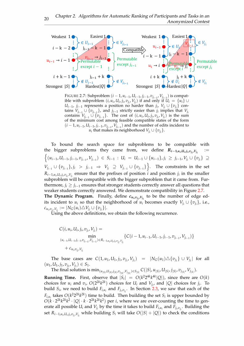
20Chapter 2. Algorithms for Automatic Ranking of Participants and Tasks in an

Anonymized Contest

1Weakest

Strongest |𝑆|

𝑖 − k − 2

𝑖 + k − 1

∈ 𝑈𝑖−1

∉ 𝑈𝑖−1

Permutable

except 𝑖 − 1

……

……

𝑢𝑖−1 → 𝑖 − 1

1Weakest

Strongest |𝑆|

𝑖 − k − 1

𝑖 + k

∈ 𝑈𝑖

∉ 𝑈𝑖

Permutable

except 𝑖

……

……𝑢𝑖 → 𝑖

…

𝑢𝑖−1

1Easiest

Hardest|𝑄|

ji−1 − k − 1

ji−1 + k

∈ 𝑉𝑗𝑖−1

∉ 𝑉𝑗𝑖−1

Permutable

except 𝑗𝑖−1

……

……

𝑣𝑗𝑖−1 → 𝑗𝑖−1

1Easiest

|𝑄|

ji + k

∈ 𝑉𝑗𝑖

∉ 𝑉𝑗𝑖

Permutable

except 𝑗𝑖

……

……𝑣𝑗𝑖 → 𝑗𝑖

…𝑉𝑗𝑖−1

ji − k − 1Compatible

Hardest

FIGURE 2.7: Subproblem (i− 1, ui−1, Ui−1, ji−1, vji−1 , Vji−1) is compat-ible with subproblem (i, ui, Ui, ji, vji , Vji ) if and only if Ui = ui ∪Ui−1, ji−1 represents a position no harder than ji, Vji ∪ vji con-tains Vji−1 ∪ vji−1, and ji−1 strictly easier than ji implies that Vjicontains Vji−1 ∪ vji−1. The cost of (i, ui, Ui, ji, vji , Vji ) is the sumof the minimum cost among feasible compatible states of the form(i− 1, ui−1, Ui−1, ji−1, vji−1 , Vji−1) and the number of edits incident to

ui that makes its neighborhood Vji ∪ vji.

To bound the search space for subproblems to be compatible withthe bigger subproblems they came from, we define Ri−1,ui ,Ui ,ji ,vji ,Vji

:=(ui−1, Ui−1, ji−1, vji−1 , Vji−1) ∈ Si−1 : Ui = Ui−1 ∪ ui−1, ji ≥ ji−1, Vji ∪ vji ⊇

Vji−1 ∪ vji−1, ji > ji−1 ⇒ Vji ⊇ Vji−1 ∪ vji−1

. The constraints in the setRi−1,ui ,Ui ,ji ,vji ,Vji

ensure that the prefixes of position i and position ji in the smallersubproblem will be compatible with the bigger subproblem that it came from. Fur-thermore, ji ≥ ji−1 ensures that stronger students correctly answer all questions thatweaker students correctly answered. We demonstrate compatibility in Figure 2.7.The Dynamic Program. Finally, define cui ,vji ,Vji

to be the number of edge ed-its incident to ui so that the neighborhood of ui becomes exactly Vji ∪ vji, i.e.,cui ,vji ,Vji

:= |NG(ui)4Vji ∪ vji|.Using the above definitions, we obtain the following recurrence.

C(i, ui, Ui, ji, vji , Vji) =

min(ui−1,Ui−1,ji−1,vji−1

,Vji−1)∈Ri−1,ui ,Ui ,ji ,vji

,Vji

C(i− 1, ui−1, Ui−1, ji−1, vji−1 , Vji−1)

+ cui ,vji ,Vji

The base cases are C(1, u1, U1, j1, vj1 , Vj1) = |NG(u1)4vj1 ∪ Vj1 | for all(u1, U1, j1, vj1 , Vj1) ∈ S1.

The final solution is min(u|S|,U|S|,j|S|,vj|S| ,Vj|S| )∈S|S| C(|S|, u|S|, U|S|, j|S|, vj|S| , Vj|S|).

Running Time. First, observe that |Si| = O(k224kk4k|Q|), since there are O(k)choices for ui and vi, O(22kk2k) choices for Ui and Vji , and |Q| choices for ji. Tobuild Si, we need to build Fi,ui and Fji ,vji

. In Section 2.3, we saw that each of theFi,ui takes O(k222kk2k) time to build. Then building the set Si is upper bounded byO(k · 22kk2kk2 · |Q| · k · 22kk2kk2) per i, where we are over-counting the time to gen-erate all possible Ui and Vji by the time it takes to build Fi,ui and Fji ,vji

. Building theset Ri−1,ui ,Ui ,ji ,vji ,Vji

while building Si will take O(|S| + |Q|) to check the conditions

2.4. Conclusion 21

that restrict Si−1 to Ri−1,ui ,Ui ,ji ,vji ,Vji. Due to the size of Si, the construction of sets

will still be dominated by the time to solve the dynamic program. Specifically, eachsubproblem (i, ui, Ui, ji, vji , Vji) takes O(|Ri−1,ui ,Ui ,ji ,vji ,Vji

|) time. So the total time isO(∑i∈S,(ui ,Ui ,ji ,vji ,Vji )∈Si

|Ri−1,ui ,Ui ,ji ,vji ,Vji|) = O(|S||Si||Si−1|) = O(n(k2 · 24kk4kn)2) =

O(n328kk8k+4).

2.3.3.0.2 Both k-near Addition

To solve the Addition version, we apply the method from the solution for Bothk-near Editing.

Theorem 2.3.7 (Both k-near Addition). Both k-near Addition can be solved in timeO(n328kk8k+4).

Proof. We redefine C(i, ui, Ui, ji, vji , Vji) to be the smallest number of edges incidentto the weakest i students that must be added so that student ui is in position i, Ui isthe set of the i− 1 weakest students, ji is the position of the hardest question correctlyanswered by Ui ∪ ui, vji is the question in position ji, and Vji is the set of the ji − 1easiest questions.

We keep Pi,ui and Fi,ui the same as in the proof for Constrained k-near Edit-

ing. Redefine Si :=(ui, Ui, ji, vji , Vji) : ui ∈

[max1, i − k, min|S|, i +

k], Ui \

[1, max1, i − k − 1

]∈ Fi,ui , vji ∈

[max1, ji − k, min|Q|, ji + k

], Vji \[

1, max1, ji − k− 1]∈ Fji ,vji

, Vji ∪ vji ⊇ NG(ui ∪Ui)

. The addition constraint

Vji ∪ vji ⊇ NG(ui ∪ Ui) is added here to ensure that the interval property in-duced by the current student ordering is satisfied every step. It was not neededin section 2.3.3.0.1 because existing edges to questions outside Vji ∪ vji could bedeleted. The definition of Ri−1,ui ,Ui ,ji ,vji ,Vji

remains the same as section 2.3.3.0.1, butusing the newly defined Si−1. Lastly, redefine cui ,vji ,Vji

to be the number of edge ad-ditions incident to ui so that the neighborhood of ui becomes exactly Vji ∪ vji, i.e.,cui ,vji ,Vji

:= |Vji ∪ vji \ NG(ui)|.The general recurrence relation of Section 2.3.3.0.1 stays the same. The base cases

change to C(1, u1, U1, j1, vj1 , Vj1) = |vj1 ∪ Vj1 \ NG(u1)|, with the convention thatj1 = 0 means Vj1 = ∅ and vj1 is omitted from the count |vj1 ∪Vj1 |.

Although the time to construct Si is larger by a factor of |Q|, the total run time isdominated by the dynamic program, which takes O(n328kk8k+4).

It is possible that the above running times for the five “easy” problems couldimprove. Our dynamic programs are designed based on the intuitiveness of thestates and not necessarily optimized for time complexity.

2.4 Conclusion

We proposed a new set of problems that arise naturally from ranking partici-pants and tasks in competitive settings and classified the complexity of each prob-lem. First, we introduced six k-near variants of the Chain Editing problem, whichcapture a common scenario of having partial information about the final orderingsfrom past rankings. Second, we provided polynomial time algorithms for five of theproblems and showed NP-hardness and an O(kn) additive approximation for theremaining one.

22Chapter 2. Algorithms for Automatic Ranking of Participants and Tasks in an

Anonymized Contest

Some open questions still remain for the NP-hard problems in Figure 2.2. ForChain Editing when both sides are unconstrained, there are no known approxima-tion algorithms. For the corresponding Chain Addition problem, can a constantapproximation can be achieved? For the Unconstrained k-near Editing problem, canthe O(kn) additive approximation be improved?

AcknowledgmentsThis work was supported in part by the US National Science Foundation underaward numbers CCF-1527032, CCF-1655442, and IIS-1553547.

23

Chapter 3

Inventory Routing on Line Metrics

3.1 Introduction

The inventory routing problem (IRP) has been studied extensively in supplychain optimization [23, 29, 25, 26]. It models the delivering decisions that a sup-plier must make to satisfy demands for its product at various locations over a timehorizon. For instance, a chain store may have different levels of demand for a prod-uct depending on the location of the store. As the product sells, each location needsto be replenished to satisfy future demands. The supplier is asked by the chain storeto decide when and how much of its product to ship to each location. Storing extraamounts of the product over time incurs holding cost while each delivery to differ-ent locations from the supply center incurs routing cost. The supplier would liketo minimize its total shipping cost and storage cost over the time horizon. Visitingfrequently incurs high routing cost while visiting sparsely incurs high holding cost.Minimizing the total cost requires finding the right trade off between the two costs.

We now give the formal definition of IRP. In IRP, we are given a complete graphKn = (V, E) whose vertices are potential locations of clients and whose edge weightsare determined by a metric w : E → R≥0 (wxz ≤ wxy + wyz for all x, y, z ∈ V). In agraph metric, the distance between every pair of vertices is the length of the shortestpath between them in a given weighted graph. There is a depot r ∈ V from whicha vehicle loads supply to drop off to clients. The vehicle may carry any amount ofsupply from the depot at each time. We have a discrete time horizon 1, . . . , T overwhich client v ∈ V demands dv

t ≥ 0 units of supply to be delivered to it by time t.For each client v ∈ V, demand time t ∈ [T], and potential serving time s ≤ t, storingone unit of supply at v during time [s, t] incurs a holding cost of hv

s,t. We assume thatthe holding costs are monotone, i.e., hv

s1,t ≥ hvs2,t for every client v ∈ V, t ∈ [T], and

s1 ≤ s2. We denote by D(V × [T]) the set points (v, t) such that dvt > 0. When the

context of V and [T] are clear, we use D and D(V × [T]) interchangeably. We callsuch points demand points. The objective is to select a tour from r through a subset ofclients per time t ∈ [T] to satisfy every demand point (no late delivery allowed) sothat the total routing cost and holding cost over [T] is minimized. For simplicity, weassume that the route is a Steiner tree (instead of a tour) through the selected subsetof clients each day since previous work in approximation algorithms for IRP assumethe same. Observe that a Steiner tree can be converted into a tour of twice its cost bydoubling the tree’s edges and short-cutting. Denote by Hv

s,t the holding cost incurredif dv

t is served at time s, i.e., Hvs,t = hv

s,tdvt . We remark that there is always an optimal

solution such that each dvt is served at a single time, for if dv

t is delivered in separateportions at times s1 < . . . < sl , then the total cost does not increase if we move all ofdv

t to be delivered at time sl .In this chapter, we construct constant factor approximation algorithms (polynomial

24 Chapter 3. Inventory Routing on Line Metrics

time algorithms producing solution within a guaranteed factor of the cost of an opti-mal solution) for IRP restricted to line metrics. First, we show a 5-approximation forIRP on line metrics with a simple rounding method. Second, we provide a primaldual algorithm for IRP on line metrics, proving a 26-approximation. The line metricinduces the distance between each pair of vertices to be the total weight of the edgesbetween them on a given weighted line. Although there is a dynamic program [18]for the line metric case of IRP, we study LP based methods as they are more gener-alizable to harder metrics. Our primal dual algorithm extends the method [67] forthe closely related joint replenishment problem (JRP) to IRP on the line to obtain a26-approximation.

The remaining sections are organized as follows. In Section 4.2, we summarizeknown approximation algorithms, heuristics, and policies for IRP. In Section 3.3, weprovide a 5-approximation for IRP on line metrics via LP rounding. In Section 3.4,we show a 26-approximation by a primal dual method for IRP on line metrics. InSection 3.5, we state related open questions.

3.2 Related Work

Approximation algorithms for special cases of IRP have been studied while thegeneral problem has no known constant factor approximation. IRP on general met-rics has a O( log T

log log T )-approximation by Nagarajan and Shi [73] and an O(log N)-approximation by Fukunaga et al [49]. For IRP restricted to nested periodic sched-ules, Fukunaga et al. [49] provide a 2.55-approximation. The joint replenishmentproblem is equivalent to IRP on a two-level tree metric, where the first level has onlyone edge. For JRP, Levi et al. [67] give a 2-approximation via a primal dual approach.They reduced the approximation factor to 1.8 in [68] by LP rounding. Recently, Bi-enkowski et al. [17] improve the factor to 1.791 by randomized rounding. For theonline version of JRP, Buchbinder et al. [22] give a 3-approximation by a differentprimal dual method. A generalization of the JRP is IRP on arbitary trees, for whichCheung et el. [32] provide a 3-approximation.

Heuristics for IRP and its variants have been extensively studied. For instance,Federgruen and Zipkin [45] study both stochastic and deterministic IRP with capaci-tated vehicles using a single day approach to initialize a feasible solution and switchclients between routes to reduce the cost. In a different single day approach, Goldenet al. [56] determine the client set per day by the urgency level of each client. Chienet al. [33] study a single day approach that passes information between consecutivedays. They seek to maximize daily profit, where the profit is determined by the rev-enue gained from the quantity delivered and the revenue lost from not satisfyingdemands, but unsatisfied demand for one day is recalculated as revenue gain forthe next day. In a short term planning approach for IRP with capacitated storagelocations, Dror et al. [40, 41] find the next best replenishment day per client for eachshort term period based on the routing cost and stockout cost. For stochastic IRP,Jaillet et al. [12, 13, 61] find the best replenishment day per client within every twoweek period, assigning only the first week’s solution, and re-solving the next twoweeks.

Researchers have also developed policies for IRP by restricting the structure ofthe routes. Kleywegt et al. [66] consider the stochastic IRP with stockout penaltiesunder the restriction that the vehicle must visit the depot after each client visit. Fordeterministic IRP, Anily and Federgruen [5] break the client set into regions and

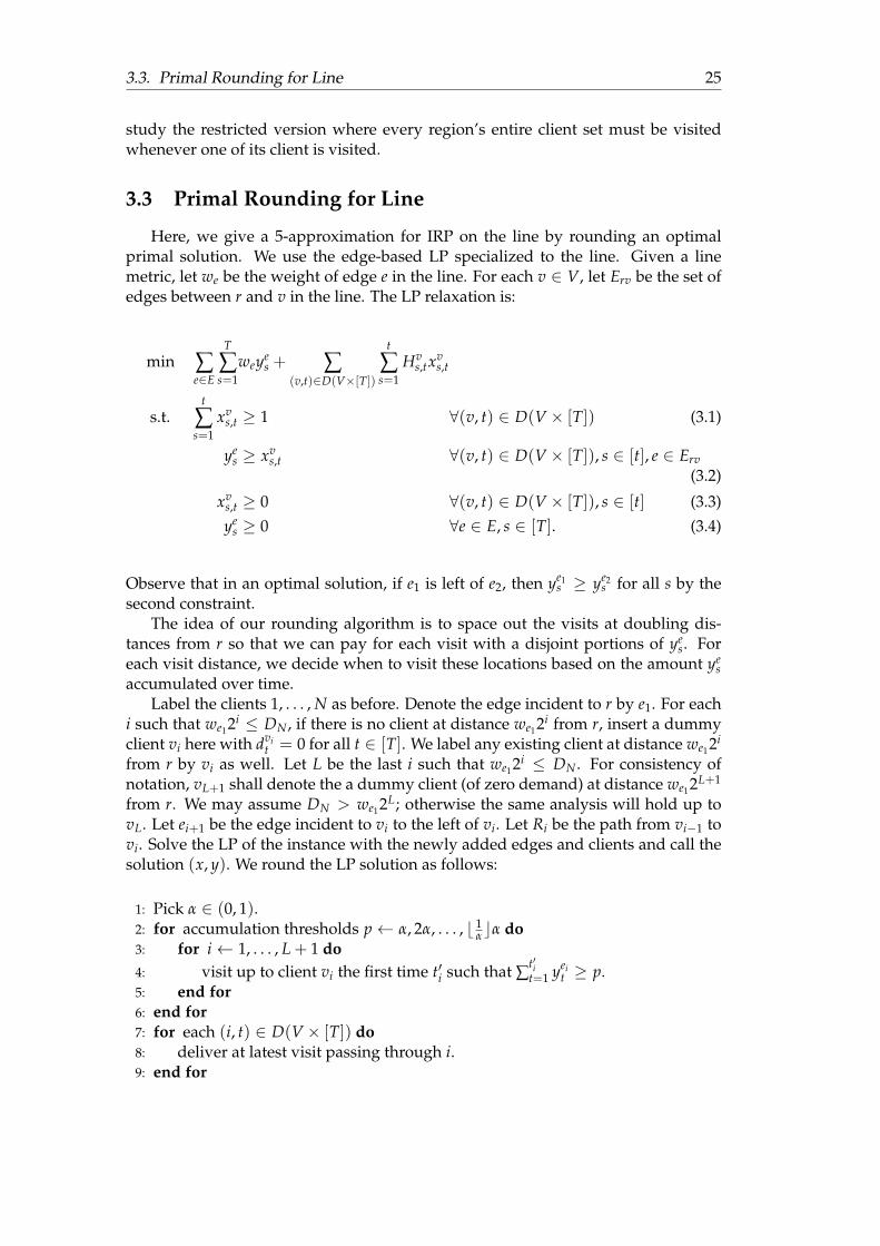
3.3. Primal Rounding for Line 25

study the restricted version where every region’s entire client set must be visitedwhenever one of its client is visited.

3.3 Primal Rounding for Line

Here, we give a 5-approximation for IRP on the line by rounding an optimalprimal solution. We use the edge-based LP specialized to the line. Given a linemetric, let we be the weight of edge e in the line. For each v ∈ V, let Erv be the set ofedges between r and v in the line. The LP relaxation is:

min ∑e∈E

T

∑s=1

weyes + ∑

(v,t)∈D(V×[T])

t

∑s=1

Hvs,tx

vs,t

s.t.t

∑s=1

xvs,t ≥ 1 ∀(v, t) ∈ D(V × [T]) (3.1)

yes ≥ xv

s,t ∀(v, t) ∈ D(V × [T]), s ∈ [t], e ∈ Erv(3.2)

xvs,t ≥ 0 ∀(v, t) ∈ D(V × [T]), s ∈ [t] (3.3)ye

s ≥ 0 ∀e ∈ E, s ∈ [T]. (3.4)

Observe that in an optimal solution, if e1 is left of e2, then ye1s ≥ ye2

s for all s by thesecond constraint.

The idea of our rounding algorithm is to space out the visits at doubling dis-tances from r so that we can pay for each visit with a disjoint portions of ye

s. Foreach visit distance, we decide when to visit these locations based on the amount ye

saccumulated over time.

Label the clients 1, . . . , N as before. Denote the edge incident to r by e1. For eachi such that we12i ≤ DN , if there is no client at distance we12i from r, insert a dummyclient vi here with dvi

t = 0 for all t ∈ [T]. We label any existing client at distance we12i

from r by vi as well. Let L be the last i such that we12i ≤ DN . For consistency ofnotation, vL+1 shall denote the a dummy client (of zero demand) at distance we12L+1

from r. We may assume DN > we12L; otherwise the same analysis will hold up tovL. Let ei+1 be the edge incident to vi to the left of vi. Let Ri be the path from vi−1 tovi. Solve the LP of the instance with the newly added edges and clients and call thesolution (x, y). We round the LP solution as follows:

1: Pick α ∈ (0, 1).2: for accumulation thresholds p← α, 2α, . . . , b 1

αcα do3: for i← 1, . . . , L + 1 do4: visit up to client vi the first time t′i such that ∑

t′it=1 yei

t ≥ p.5: end for6: end for7: for each (i, t) ∈ D(V × [T]) do8: deliver at latest visit passing through i.9: end for

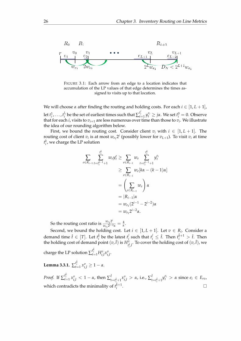
26 Chapter 3. Inventory Routing on Line Metrics

FIGURE 3.1: Each arrow from an edge to a location indicates thataccumulation of the LP values of that edge determines the times as-

signed to visits up to that location.

We will choose α after finding the routing and holding costs. For each i ∈ [1, L + 1],

let t1i , . . . , tli

i be the set of earliest times such that ∑tji

t=1 yeit ≥ jα. We set t0

i = 0. Observethat for each i, visits to vi+1 are less numerous over time than those to vi. We illustratethe idea of our rounding algorithm below.

First, we bound the routing cost. Consider client vi with i ∈ [1, L + 1]. Therouting cost of client vi is at most we12i (possibly lower for vL+1). To visit vi at timetki , we charge the LP solution

∑e∈Ri−1

tki

∑t=tk−1

i +1

weyet ≥ ∑

e∈Ri−1

we

tki

∑t=tk−1

i +1

yeit

≥ ∑e∈Ri−1

we[kα− (k− 1)α]

=

(∑

e∈Ri−1

we

)α

= |Ri−1|α= we1(2

i−1 − 2i−2)α

= we12i−2α.

So the routing cost ratio iswe1 2i

we1 2i−2α= 4

α .

Second, we bound the holding cost. Let i ∈ [1, L + 1]. Let v ∈ Ri. Consider ademand time t ∈ [T]. Let tk

i be the latest tji such that tj

i ≤ t. Then tk+1i > t. Then

the holding cost of demand point (v, t) is Hvtki ,t

. To cover the holding cost of (v, t), we

charge the LP solution ∑tki

t=1Hvt,tx

vt,t.

Lemma 3.3.1. ∑tki

t=1 xvt,t ≥ 1− α.

Proof. If ∑tki

t=1 xvt,t < 1− α, then ∑t

t=tki +1

xvt,t > α, i.e., ∑t

t=tki +1

yeit > α since ei ∈ Erv,

which contradicts the minimality of tk+1i .

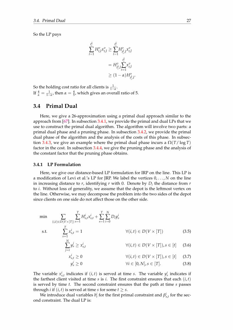
3.4. Primal Dual 27

So the LP pays

tki

∑t=1

Hvt,tx

vt,t ≥

tki

∑t=1

Hvtki ,t

xvt,t

= Hvtki ,t

tki

∑t=1

xvt,t

≥ (1− α)Hvtki ,t

.

So the holding cost ratio for all clients is 11−α .

If 4α = 1

1−α , then α = 45 , which gives an overall ratio of 5.

3.4 Primal Dual

Here, we give a 26-approximation using a primal dual approach similar to theapproach from [67]. In subsection 3.4.1, we provide the primal and dual LPs that weuse to construct the primal dual algorithm. The algorithm will involve two parts: aprimal dual phase and a pruning phase. In subsection 3.4.2, we provide the primaldual phase of the algorithm and the analysis of the costs of this phase. In subsec-tion 3.4.3, we give an example where the primal dual phase incurs a Ω(T/ log T)factor in the cost. In subsection 3.4.4, we give the pruning phase and the analysis ofthe constant factor that the pruning phase obtains.

3.4.1 LP Formulation

Here, we give our distance-based LP formulation for IRP on the line. This LP isa modification of Levi et al.’s LP for JRP. We label the vertices 0, . . . , N on the linein increasing distance to r, identifying r with 0. Denote by Di the distance from rto i. Without loss of generality, we assume that the depot is the leftmost vertex onthe line. Otherwise, we may decompose the problem into the two sides of the depotsince clients on one side do not affect those on the other side.

min ∑(i,t)∈D(V×[T])

T

∑s=1

His,tx

is,t +

T

∑s=1

N

∑i=0

Diyis

s.t.T

∑s=1

xis,t = 1 ∀(i, t) ∈ D(V × [T]) (3.5)

N

∑j=i

yjs ≥ xi

s,t ∀(i, t) ∈ D(V × [T]), s ∈ [t] (3.6)

xis,t ≥ 0 ∀(i, t) ∈ D(V × [T]), s ∈ [t] (3.7)

yis ≥ 0 ∀i ∈ [0, N], s ∈ [T]. (3.8)

The variable xis,t indicates if (i, t) is served at time s. The variable yi

s indicates ifthe farthest client visited at time s is i. The first constraint ensures that each (i, t)is served by time t. The second constraint ensures that the path at time s passesthrough i if (i, t) is served at time s for some t ≥ s.

We introduce dual variables bit for the first primal constraint and βi

s,t for the sec-ond constraint. The dual LP is:

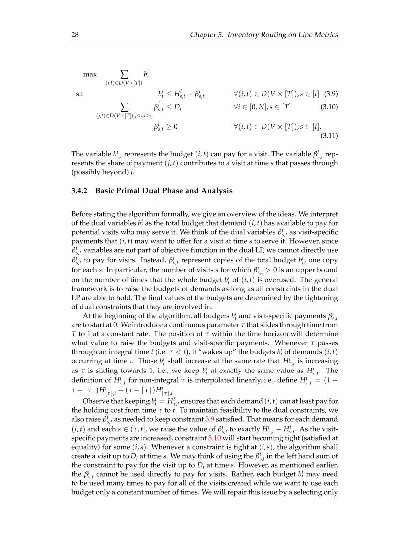
28 Chapter 3. Inventory Routing on Line Metrics

max ∑(i,t)∈D(V×[T])

bit

s.t bit ≤ Hi

s,t + βis,t ∀(i, t) ∈ D(V × [T]), s ∈ [t] (3.9)

∑(j,t)∈D(V×[T]):j≤i,t≥s

βjs,t ≤ Di ∀i ∈ [0, N], s ∈ [T] (3.10)

βis,t ≥ 0 ∀(i, t) ∈ D(V × [T]), s ∈ [t].

(3.11)

The variable bis,t represents the budget (i, t) can pay for a visit. The variable β

js,t rep-

resents the share of payment (j, t) contributes to a visit at time s that passes through(possibly beyond) j.

3.4.2 Basic Primal Dual Phase and Analysis

Before stating the algorithm formally, we give an overview of the ideas. We interpretof the dual variables bi

t as the total budget that demand (i, t) has available to pay forpotential visits who may serve it. We think of the dual variables βi

s,t as visit-specificpayments that (i, t) may want to offer for a visit at time s to serve it. However, sinceβi

s,t variables are not part of objective function in the dual LP, we cannot directly useβi

s,t to pay for visits. Instead, βis,t represent copies of the total budget bi

t, one copyfor each s. In particular, the number of visits s for which βi

s,t > 0 is an upper boundon the number of times that the whole budget bi

t of (i, t) is overused. The generalframework is to raise the budgets of demands as long as all constraints in the dualLP are able to hold. The final values of the budgets are determined by the tighteningof dual constraints that they are involved in.

At the beginning of the algorithm, all budgets bit and visit-specific payments βi

s,tare to start at 0. We introduce a continuous parameter τ that slides through time fromT to 1 at a constant rate. The position of τ within the time horizon will determinewhat value to raise the budgets and visit-specific payments. Whenever τ passesthrough an integral time t (i.e. τ < t), it “wakes up” the budgets bi

t of demands (i, t)occurring at time t. Those bi

t shall increase at the same rate that Hiτ,t is increasing

as τ is sliding towards 1, i.e., we keep bit at exactly the same value as Hi

τ,t. Thedefinition of Hi

τ,t for non-integral τ is interpolated linearly, i.e., define Hiτ,t = (1−

τ + bτc)Hibτc,t + (τ − bτc)Hi

dτe,t.

Observe that keeping bit = Hi

τ,t ensures that each demand (i, t) can at least pay forthe holding cost from time τ to t. To maintain feasibility to the dual constraints, wealso raise βi

s,t as needed to keep constraint 3.9 satisfied. That means for each demand(i, t) and each s ∈ (τ, t], we raise the value of βi

s,t to exactly Hiτ,t − Hi

s,t. As the visit-specific payments are increased, constraint 3.10 will start becoming tight (satisfied atequality) for some (i, s). Whenever a constraint is tight at (i, s), the algorithm shallcreate a visit up to Di at time s. We may think of using the βi

s,t in the left hand sum ofthe constraint to pay for the visit up to Di at time s. However, as mentioned earlier,the βi

s,t cannot be used directly to pay for visits. Rather, each budget bit may need

to be used many times to pay for all of the visits created while we want to use eachbudget only a constant number of times. We will repair this issue by a selecting only

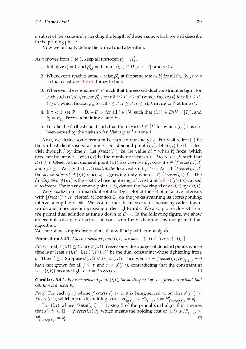
3.4. Primal Dual 29

a subset of the visits and extending the length of those visits, which we will describein the pruning phase.

Now we formally define the primal dual algorithm.

As τ moves from T to 1, keep all unfrozen bit = Hi

τt.

1. Initialize bit = 0 and βi

s,t = 0 for all (i, t) ∈ D(V × [T]) and s ≤ t.

2. Whenever τ reaches some s, raise βist at the same rate as bi

t for all i ∈ [N], t ≥ sso that constraint 3.9 continues to hold.

3. Whenever there is some i∗, s∗ such that the second dual constraint is tight, foreach such (i∗, s∗), freeze β

js∗t for all j ≤ i∗, t ≥ s∗ (which freezes bj

t for all j ≤ i∗,t ≥ s∗, which freezes β

jst for all j ≤ i∗, t ≥ s∗, s ≤ τ). Visit up to i∗ at time s∗.

4. If τ < 1, set βi11 = Di − Di−1 for all i ∈ [N] such that (i, 1) ∈ D(V × [T]), and

bi1 = βi

11. Freeze remaining bit and βi

st.

5. Let i be the farthest client such that there exists t ∈ [T] for which (i, t) has notbeen served by the visits so far. Visit up to i at time 1.

Next, we define some terms to be used in our analysis. For visit s, let i(s) bethe farthest client visited at time s. For demand point (i, t), let s(i, t) be the latestvisit through i by time t. Let f reeze(i, t) be the value of τ when bi

t froze, whichneed not be integer. Let µ(i, t) be the number of visits s ∈ [ f reeze(i, t), t] such thati(s) ≥ i. Observe that demand point (i, t) has positive βi

s,t only if s ∈ [ f reeze(i, t), t]and i(s) ≥ i. We say that (i, t) contributes to a visit s if βi

s,t > 0. We call [ f reeze(i, t), t]the active interval of (i, t) since bi

t is growing only when τ ∈ [ f reeze(i, t), t]. Thefreezing visit of (i, t) is the visit s whose tightening of constraint 3.10 at (i(s), s) causedbi

t to freeze. For every demand point (i, t), denote the freezing visit of (i, t) by s′(i, t).We visualize our primal dual solution by a plot of the set of all active intervals

with [ f reeze(i, t), t] plotted at location Di on the y-axis spanning its correspondinginterval along the x-axis. We assume that distances are in increasing order down-wards and times are in increasing order rightwards. We also plot each visit fromthe primal dual solution at time s down to Di(s). In the following figure, we showan example of a plot of active intervals with the visits grown by our primal dualalgorithm.We state some simple observations that will help with our analysis.

Proposition 3.4.1. Given a demand point (i, t), we have s′(i, t) ∈ [ f reeze(i, t), t].

Proof. First, s′(i, t) ≤ t since s′(i, t) freezes only the budges of demand points whosetime is at least s′(i, t). Let (i′, s′(i, t)) be the dual constraint whose tightening frozebi

t. Then i′ ≥ i. Suppose s′(i, t) < f reeze(i, t). Then when τ = f reeze(i, t), βjs′(i,t),r = 0

have not grown for all j ≤ i′ and r ≥ s′(i, t), contradicting that the constraint at(i′, s′(i, t)) became tight at τ = f reeze(i, t).

Corollary 3.4.2. For each demand point (i, t), the holding cost of (i, t) from our primal dualsolution is at most bi

t.

Proof. For each (i, t) whose f reeze(i, t) > 1, it is being served at or after s′(i, t) ≥f reeze(i, t), which means its holding cost is Hi

s(i,t),t ≤ His′(i,t),t <= Hi

f reeze(i,t),t = bit.

For (i, t) whose f reeze(i, t) = 1, step 5 of the primal dual algorithm ensuresthat s(i, t) ∈ [1 = f reeze(i, t), t], which means the holding cost of (i, t) is Hi

s(i,t),t ≤Hi

f reeze(i,t),t = bit.

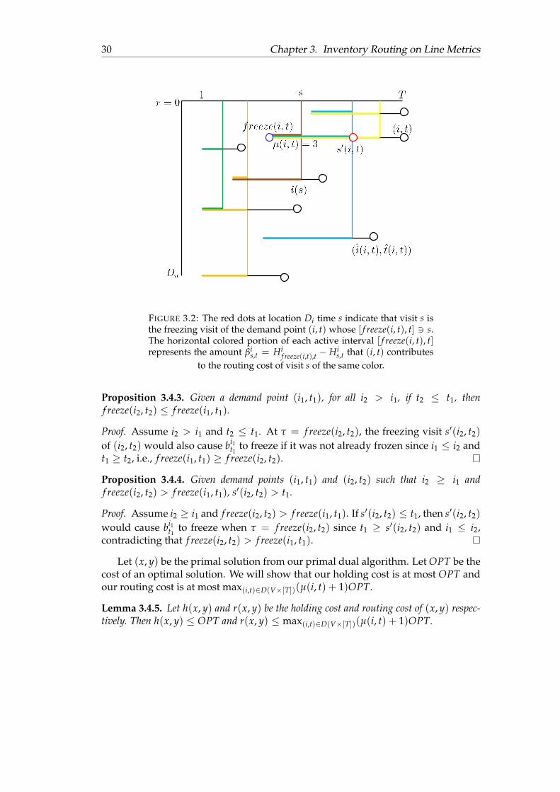
30 Chapter 3. Inventory Routing on Line Metrics

FIGURE 3.2: The red dots at location Di time s indicate that visit s isthe freezing visit of the demand point (i, t) whose [ f reeze(i, t), t] 3 s.The horizontal colored portion of each active interval [ f reeze(i, t), t]represents the amount βi

s,t = Hif reeze(i,t),t − Hi

s,t that (i, t) contributesto the routing cost of visit s of the same color.

Proposition 3.4.3. Given a demand point (i1, t1), for all i2 > i1, if t2 ≤ t1, thenf reeze(i2, t2) ≤ f reeze(i1, t1).

Proof. Assume i2 > i1 and t2 ≤ t1. At τ = f reeze(i2, t2), the freezing visit s′(i2, t2)

of (i2, t2) would also cause bi1t1

to freeze if it was not already frozen since i1 ≤ i2 andt1 ≥ t2, i.e., f reeze(i1, t1) ≥ f reeze(i2, t2).

Proposition 3.4.4. Given demand points (i1, t1) and (i2, t2) such that i2 ≥ i1 andf reeze(i2, t2) > f reeze(i1, t1), s′(i2, t2) > t1.

Proof. Assume i2 ≥ i1 and f reeze(i2, t2) > f reeze(i1, t1). If s′(i2, t2) ≤ t1, then s′(i2, t2)

would cause bi1t1

to freeze when τ = f reeze(i2, t2) since t1 ≥ s′(i2, t2) and i1 ≤ i2,contradicting that f reeze(i2, t2) > f reeze(i1, t1).

Let (x, y) be the primal solution from our primal dual algorithm. Let OPT be thecost of an optimal solution. We will show that our holding cost is at most OPT andour routing cost is at most max(i,t)∈D(V×[T])(µ(i, t) + 1)OPT.

Lemma 3.4.5. Let h(x, y) and r(x, y) be the holding cost and routing cost of (x, y) respec-tively. Then h(x, y) ≤ OPT and r(x, y) ≤ max(i,t)∈D(V×[T])(µ(i, t) + 1)OPT.

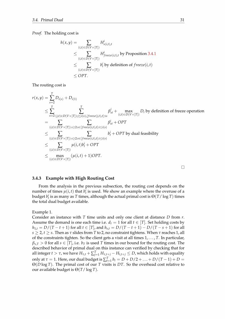
3.4. Primal Dual 31

Proof. The holding cost is

h(x, y) = ∑(i,t)∈D(V×[T])

His(i,t),t

≤ ∑(i,t)∈D(V×[T])

Hif reeze(i,t),t by Proposition 3.4.1

≤ ∑(i,t)∈D(V×[T])

bit by definition of f reeze(i, t)

≤ OPT.

The routing cost is

r(x, y) =T

∑s=2

Di(s) + Di(1)

≤T

∑s=2

T

∑(j,t)∈D(V×[T]):j≤i(s),[ f reeze(j,t),t]3s

βjst + max

(i,t)∈D(V×[T])Di by definition of freeze operation

= ∑(i,t)∈D(V×[T])

∑s≥2:s∈[ f reeze(i,t),t]:i≤i(s)

βist + OPT

≤ ∑(i,t)∈D(V×[T])

∑s≥2:s∈[ f reeze(i,t),t]:i≤i(s)

bit + OPT by dual feasibility

≤ ∑(i,t)∈D(V×[T])

µ(i, t)bit + OPT

≤ max(i,t)∈D(V×[T])

(µ(i, t) + 1)OPT.

3.4.3 Example with High Routing Cost

From the analysis in the previous subsection, the routing cost depends on thenumber of times µ(i, t) that bi

t is used. We show an example where the overuse of abudget bi

t is as many as T times, although the actual primal cost is Θ(T/ log T) timesthe total dual budget available.

Example 1.Consider an instance with T time units and only one client at distance D from r.Assume the demand is one each time i.e. dt = 1 for all t ∈ [T]. Set holding costs byh1,t = D/(T− t + 1) for all t ∈ [T], and hs,t = D/(T− t + 1)− D/(T− s + 1) for alls ≥ 2, t ≥ s. Then as τ slides from T to 2, no constraint tightens. When τ reaches 1, allof the constraints tighten. So the client gets a visit at all times 1, . . . , T. In particular,βs,T > 0 for all s ∈ [T], i.e. bT is used T times in our bound for the routing cost. Thedescribed behavior of primal dual on this instance can verified by checking that forall integer t > τ, we have Hτ,t + ∑T

j=1 Hτ,t+j− Ht,t+j ≤ D, which holds with equalityonly at τ = 1. Here, our dual budget is ∑T

t=1 bt = D + D/2+ . . . + D/(T− 1) + D =Θ(D log T). The primal cost of our T visits is DT. So the overhead cost relative toour available budget is Θ(T/ log T).

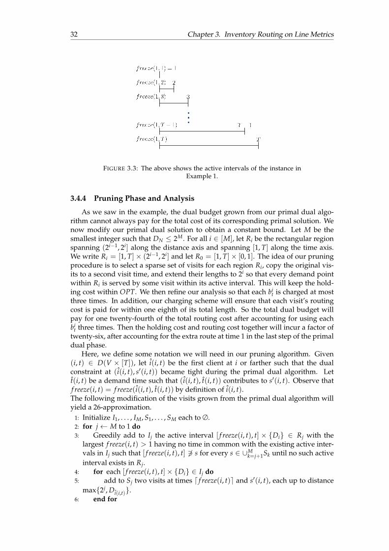
32 Chapter 3. Inventory Routing on Line Metrics

FIGURE 3.3: The above shows the active intervals of the instance inExample 1.

3.4.4 Pruning Phase and Analysis

As we saw in the example, the dual budget grown from our primal dual algo-rithm cannot always pay for the total cost of its corresponding primal solution. Wenow modify our primal dual solution to obtain a constant bound. Let M be thesmallest integer such that DN ≤ 2M. For all i ∈ [M], let Ri be the rectangular regionspanning (2i−1, 2i] along the distance axis and spanning [1, T] along the time axis.We write Ri = [1, T]× (2i−1, 2i] and let R0 = [1, T]× [0, 1]. The idea of our pruningprocedure is to select a sparse set of visits for each region Ri, copy the original vis-its to a second visit time, and extend their lengths to 2i so that every demand pointwithin Ri is served by some visit within its active interval. This will keep the hold-ing cost within OPT. We then refine our analysis so that each bi

t is charged at mostthree times. In addition, our charging scheme will ensure that each visit’s routingcost is paid for within one eighth of its total length. So the total dual budget willpay for one twenty-fourth of the total routing cost after accounting for using eachbi

t three times. Then the holding cost and routing cost together will incur a factor oftwenty-six, after accounting for the extra route at time 1 in the last step of the primaldual phase.

Here, we define some notation we will need in our pruning algorithm. Given(i, t) ∈ D(V × [T]), let i(i, t) be the first client at i or farther such that the dualconstraint at (i(i, t), s′(i, t)) became tight during the primal dual algorithm. Lett(i, t) be a demand time such that (i(i, t), t(i, t)) contributes to s′(i, t). Observe thatf reeze(i, t) = f reeze(i(i, t), t(i, t)) by definition of i(i, t).The following modification of the visits grown from the primal dual algorithm willyield a 26-approximation.

1: Initialize I1, . . . , IM, S1, . . . , SM each to ∅.2: for j← M to 1 do3: Greedily add to Ij the active interval [ f reeze(i, t), t] × Di ∈ Rj with the

largest f reeze(i, t) > 1 having no time in common with the existing active inter-vals in Ij such that [ f reeze(i, t), t] 63 s for every s ∈ ∪M

k=j+1Sk until no such activeinterval exists in Rj.

4: for each [ f reeze(i, t), t]× Di ∈ Ij do5: add to Sj two visits at times d f reeze(i, t)e and s′(i, t), each up to distance

max2j, Di(i,t).6: end for

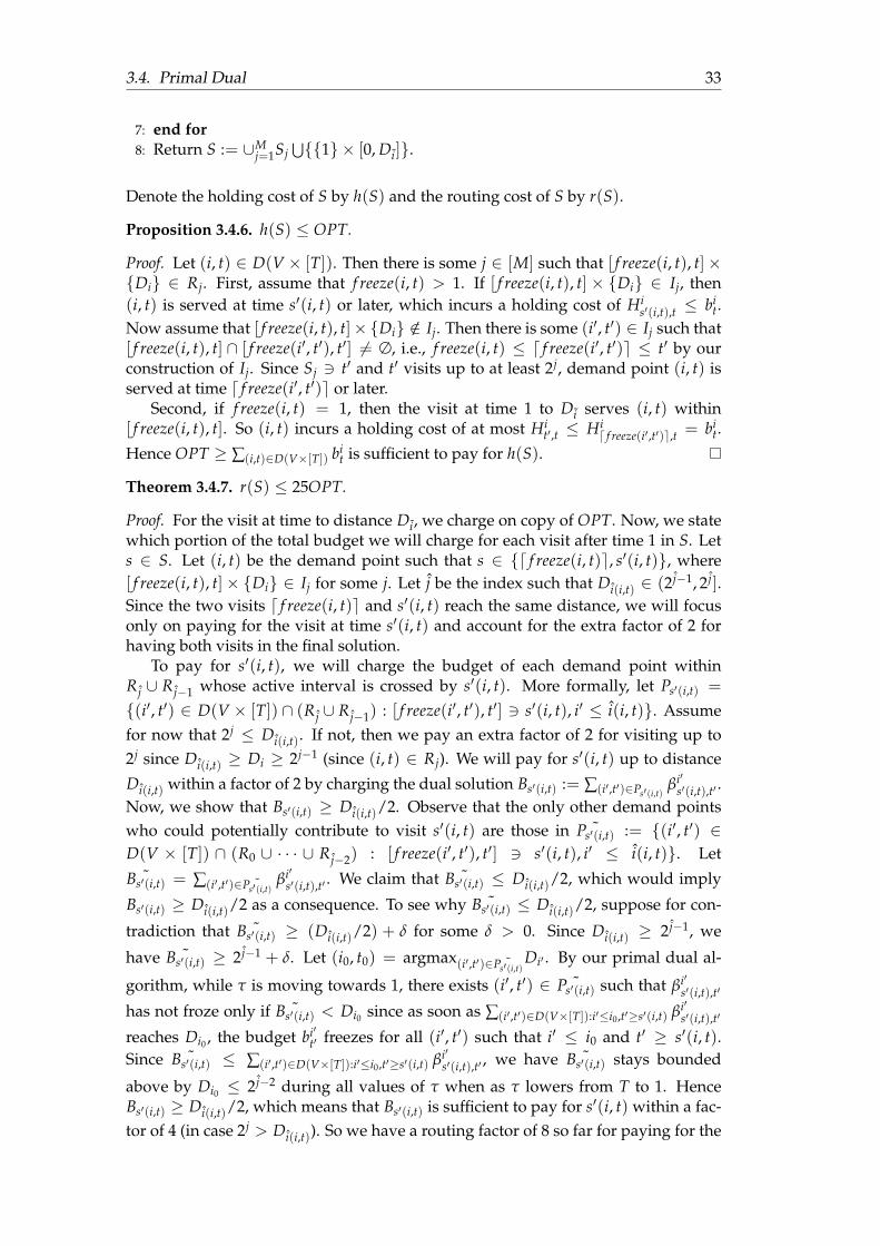
3.4. Primal Dual 33

7: end for8: Return S := ∪M

j=1Sj⋃1 × [0, Di].

Denote the holding cost of S by h(S) and the routing cost of S by r(S).

Proposition 3.4.6. h(S) ≤ OPT.

Proof. Let (i, t) ∈ D(V × [T]). Then there is some j ∈ [M] such that [ f reeze(i, t), t]×Di ∈ Rj. First, assume that f reeze(i, t) > 1. If [ f reeze(i, t), t] × Di ∈ Ij, then(i, t) is served at time s′(i, t) or later, which incurs a holding cost of Hi

s′(i,t),t ≤ bit.

Now assume that [ f reeze(i, t), t]×Di /∈ Ij. Then there is some (i′, t′) ∈ Ij such that[ f reeze(i, t), t] ∩ [ f reeze(i′, t′), t′] 6= ∅, i.e., f reeze(i, t) ≤ d f reeze(i′, t′)e ≤ t′ by ourconstruction of Ij. Since Sj 3 t′ and t′ visits up to at least 2j, demand point (i, t) isserved at time d f reeze(i′, t′)e or later.

Second, if f reeze(i, t) = 1, then the visit at time 1 to Di serves (i, t) within[ f reeze(i, t), t]. So (i, t) incurs a holding cost of at most Hi

t′,t ≤ Hid f reeze(i′,t′)e,t = bi

t.

Hence OPT ≥ ∑(i,t)∈D(V×[T]) bit is sufficient to pay for h(S).

Theorem 3.4.7. r(S) ≤ 25OPT.

Proof. For the visit at time to distance Di, we charge on copy of OPT. Now, we statewhich portion of the total budget we will charge for each visit after time 1 in S. Lets ∈ S. Let (i, t) be the demand point such that s ∈ d f reeze(i, t)e, s′(i, t), where[ f reeze(i, t), t]× Di ∈ Ij for some j. Let j be the index such that Di(i,t) ∈ (2 j−1, 2 j].Since the two visits d f reeze(i, t)e and s′(i, t) reach the same distance, we will focusonly on paying for the visit at time s′(i, t) and account for the extra factor of 2 forhaving both visits in the final solution.

To pay for s′(i, t), we will charge the budget of each demand point withinR j ∪ R j−1 whose active interval is crossed by s′(i, t). More formally, let Ps′(i,t) =

(i′, t′) ∈ D(V × [T]) ∩ (R j ∪ R j−1) : [ f reeze(i′, t′), t′] 3 s′(i, t), i′ ≤ i(i, t). Assumefor now that 2j ≤ Di(i,t). If not, then we pay an extra factor of 2 for visiting up to2j since Di(i,t) ≥ Di ≥ 2j−1 (since (i, t) ∈ Rj). We will pay for s′(i, t) up to distance

Di(i,t) within a factor of 2 by charging the dual solution Bs′(i,t) := ∑(i′,t′)∈Ps′(i,t)βi′

s′(i,t),t′ .Now, we show that Bs′(i,t) ≥ Di(i,t)/2. Observe that the only other demand pointswho could potentially contribute to visit s′(i, t) are those in ˜Ps′(i,t) := (i′, t′) ∈D(V × [T]) ∩ (R0 ∪ · · · ∪ R j−2) : [ f reeze(i′, t′), t′] 3 s′(i, t), i′ ≤ i(i, t). Let

˜Bs′(i,t) = ∑(i′,t′)∈ ˜Ps′(i,t)βi′

s′(i,t),t′ . We claim that ˜Bs′(i,t) ≤ Di(i,t)/2, which would imply

Bs′(i,t) ≥ Di(i,t)/2 as a consequence. To see why ˜Bs′(i,t) ≤ Di(i,t)/2, suppose for con-

tradiction that ˜Bs′(i,t) ≥ (Di(i,t)/2) + δ for some δ > 0. Since Di(i,t) ≥ 2 j−1, we

have ˜Bs′(i,t) ≥ 2 j−1 + δ. Let (i0, t0) = argmax(i′,t′)∈ ˜Ps′(i,t)Di′ . By our primal dual al-

gorithm, while τ is moving towards 1, there exists (i′, t′) ∈ ˜Ps′(i,t) such that βi′s′(i,t),t′

has not froze only if ˜Bs′(i,t) < Di0 since as soon as ∑(i′,t′)∈D(V×[T]):i′≤i0,t′≥s′(i,t) βi′s′(i,t),t′

reaches Di0 , the budget bi′t′ freezes for all (i′, t′) such that i′ ≤ i0 and t′ ≥ s′(i, t).

Since ˜Bs′(i,t) ≤ ∑(i′,t′)∈D(V×[T]):i′≤i0,t′≥s′(i,t) βi′s′(i,t),t′ , we have ˜Bs′(i,t) stays bounded

above by Di0 ≤ 2 j−2 during all values of τ when as τ lowers from T to 1. HenceBs′(i,t) ≥ Di(i,t)/2, which means that Bs′(i,t) is sufficient to pay for s′(i, t) within a fac-tor of 4 (in case 2j > Di(i,t)). So we have a routing factor of 8 so far for paying for the

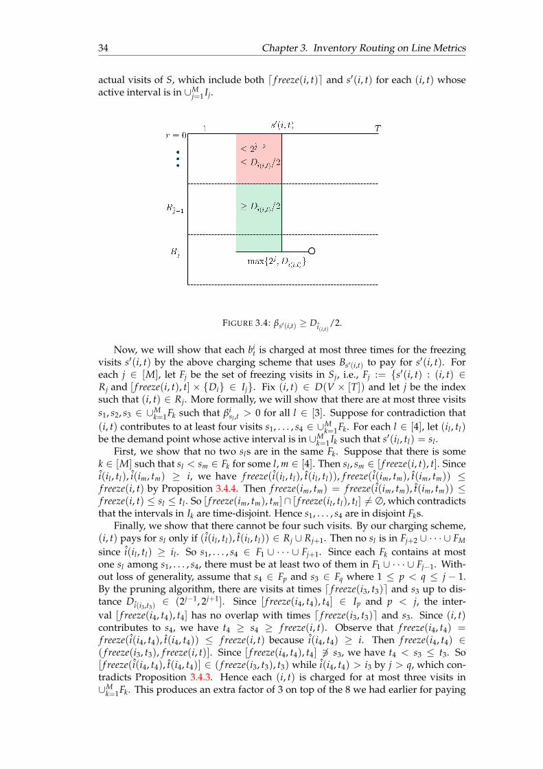
34 Chapter 3. Inventory Routing on Line Metrics

actual visits of S, which include both d f reeze(i, t)e and s′(i, t) for each (i, t) whoseactive interval is in ∪M

j=1 Ij.

FIGURE 3.4: βs′(i,t) ≥ Di(i,t)/2.

Now, we will show that each bit is charged at most three times for the freezing

visits s′(i, t) by the above charging scheme that uses Bs′(i,t) to pay for s′(i, t). Foreach j ∈ [M], let Fj be the set of freezing visits in Sj, i.e., Fj := s′(i, t) : (i, t) ∈Rj and [ f reeze(i, t), t] × Di ∈ Ij. Fix (i, t) ∈ D(V × [T]) and let j be the indexsuch that (i, t) ∈ Rj. More formally, we will show that there are at most three visitss1, s2, s3 ∈ ∪M

k=1Fk such that βisl ,t > 0 for all l ∈ [3]. Suppose for contradiction that

(i, t) contributes to at least four visits s1, . . . , s4 ∈ ∪Mk=1Fk. For each l ∈ [4], let (il , tl)

be the demand point whose active interval is in ∪Mk=1 Ik such that s′(il , tl) = sl .

First, we show that no two sls are in the same Fk. Suppose that there is somek ∈ [M] such that sl < sm ∈ Fk for some l, m ∈ [4]. Then sl , sm ∈ [ f reeze(i, t), t]. Sincei(il , tl), i(im, tm) ≥ i, we have f reeze(i(il , tl), t(il , tl)), f reeze(i(im, tm), t(im, tm)) ≤f reeze(i, t) by Proposition 3.4.4. Then f reeze(im, tm) = f reeze(i(im, tm), t(im, tm)) ≤f reeze(i, t) ≤ sl ≤ tl . So [ f reeze(im, tm), tm]∩ [ f reeze(il , tl), tl ] 6= ∅, which contradictsthat the intervals in Ik are time-disjoint. Hence s1, . . . , s4 are in disjoint Fks.

Finally, we show that there cannot be four such visits. By our charging scheme,(i, t) pays for sl only if (i(il , tl), t(il , tl)) ∈ Rj ∪ Rj+1. Then no sl is in Fj+2 ∪ · · · ∪ FM

since i(il , tl) ≥ il . So s1, . . . , s4 ∈ F1 ∪ · · · ∪ Fj+1. Since each Fk contains at mostone sl among s1, . . . , s4, there must be at least two of them in F1 ∪ · · · ∪ Fj−1. With-out loss of generality, assume that s4 ∈ Fp and s3 ∈ Fq where 1 ≤ p < q ≤ j − 1.By the pruning algorithm, there are visits at times d f reeze(i3, t3)e and s3 up to dis-tance Di(i3,t3)

∈ (2j−1, 2j+1]. Since [ f reeze(i4, t4), t4] ∈ Ip and p < j, the inter-val [ f reeze(i4, t4), t4] has no overlap with times d f reeze(i3, t3)e and s3. Since (i, t)contributes to s4, we have t4 ≥ s4 ≥ f reeze(i, t). Observe that f reeze(i4, t4) =f reeze(i(i4, t4), t(i4, t4)) ≤ f reeze(i, t) because i(i4, t4) ≥ i. Then f reeze(i4, t4) ∈( f reeze(i3, t3), f reeze(i, t)]. Since [ f reeze(i4, t4), t4] 63 s3, we have t4 < s3 ≤ t3. So[ f reeze(i(i4, t4), t(i4, t4)] ∈ ( f reeze(i3, t3), t3) while i(i4, t4) > i3 by j > q, which con-tradicts Proposition 3.4.3. Hence each (i, t) is charged for at most three visits in∪M

k=1Fk. This produces an extra factor of 3 on top of the 8 we had earlier for paying

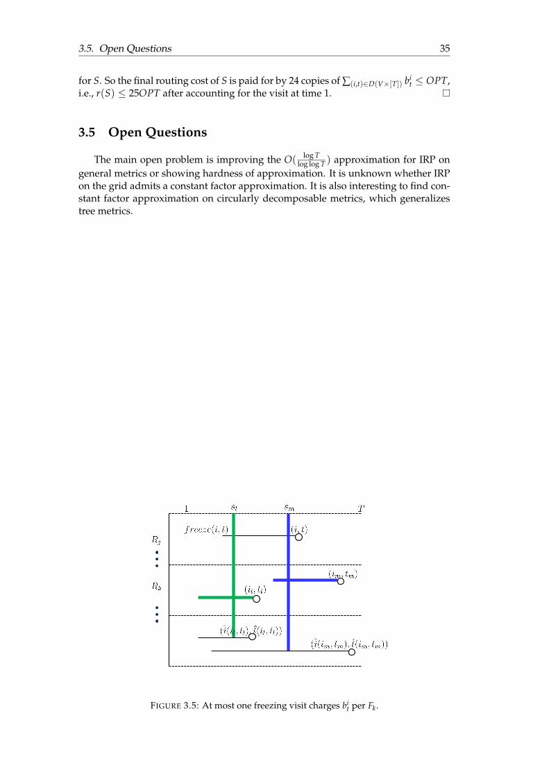
3.5. Open Questions 35

for S. So the final routing cost of S is paid for by 24 copies of ∑(i,t)∈D(V×[T]) bit ≤ OPT,

i.e., r(S) ≤ 25OPT after accounting for the visit at time 1.

3.5 Open Questions

The main open problem is improving the O( log Tlog log T ) approximation for IRP on

general metrics or showing hardness of approximation. It is unknown whether IRPon the grid admits a constant factor approximation. It is also interesting to find con-stant factor approximation on circularly decomposable metrics, which generalizestree metrics.

FIGURE 3.5: At most one freezing visit charges bit per Fk.

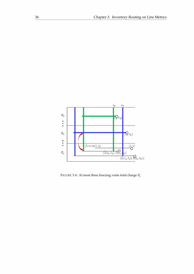
36 Chapter 3. Inventory Routing on Line Metrics

FIGURE 3.6: At most three freezing visits total charge bit.

37

Chapter 4

Combinatorial Heuristics forInventory Routing on GeneralMetrics

4.1 Introduction

The Inventory Routing Problem (IRP) arises from Vendor Managed Inventorysystems in which a product supplier and its retailers cooperate in the inventory plan-ning. First, the retailers share with the supplier the demand patterns for its productand the storage costs for keeping early deliveries per retailer location. Then the sup-plier is responsible for planning a delivery schedule that serves all the demands ontime. Naturally, the supplier wishes to minimize its routing cost and storage costover the time horizon. This optimization problem is called IRP and has been studiedextensively [23, 29, 25, 26].

In the classical single-depot IRP, a set of client demand locations in a metric con-taining the depot is given, and for a planning horizon of T days, a daily demand ateach client location is specified. The goal is to come up with vehicle routing sched-ules in each of the T days to stock the client demands before they materialize. How-ever, early stocking at a location incurs a location- and duration-specific inventoryholding cost that are also specified. If we assume the daily replenishing vehicle hasinfinite capacity, the distance traveled by the vehicle in a daily route translates to arouting cost. The goal of IRP is to find daily vehicle schedules for the T days thatdeliver enough supply at each location to meet all daily demands and minimizesthe sum of inventory holding costs for units supplied ahead of their demand andthe daily routing costs of the vehicle, over the T days.Problem Definition. We now give the formal definition of IRP. In IRP, we are givena complete graph Kn = (V, E) whose vertices are potential locations of clients andwhose edge weights are determined by a metric w : E → R≥0 (wxz ≤ wxy + wyz forall x, y, z ∈ V). In a graph metric, the distance between every pair of vertices is thelength of the shortest path between them in a given weighted graph. There is a depotr ∈ V from which a vehicle of infinite capacity loads supply to drop off to clients.The vehicle may carry any amount of supply from the depot at each time. We havea discrete time horizon 1, . . . , T over which client v ∈ V demands dv

t ≥ 0 units ofsupply to be delivered to it by time t. For each client v ∈ V, demand time t ∈ [T], andpotential serving time s ≤ t, storing one unit of supply at v during time [s, t] incursa holding cost of hv

s,t. We denote by D(V × [T]) the set points (v, t) such that dvt > 0.

When the context of V and [T] are clear, we use D and D(V × [T]) interchangeably.We call such points demand points. The objective is to select a tour from r througha subset of clients per time t ∈ [T] to satisfy every demand point (no late delivery

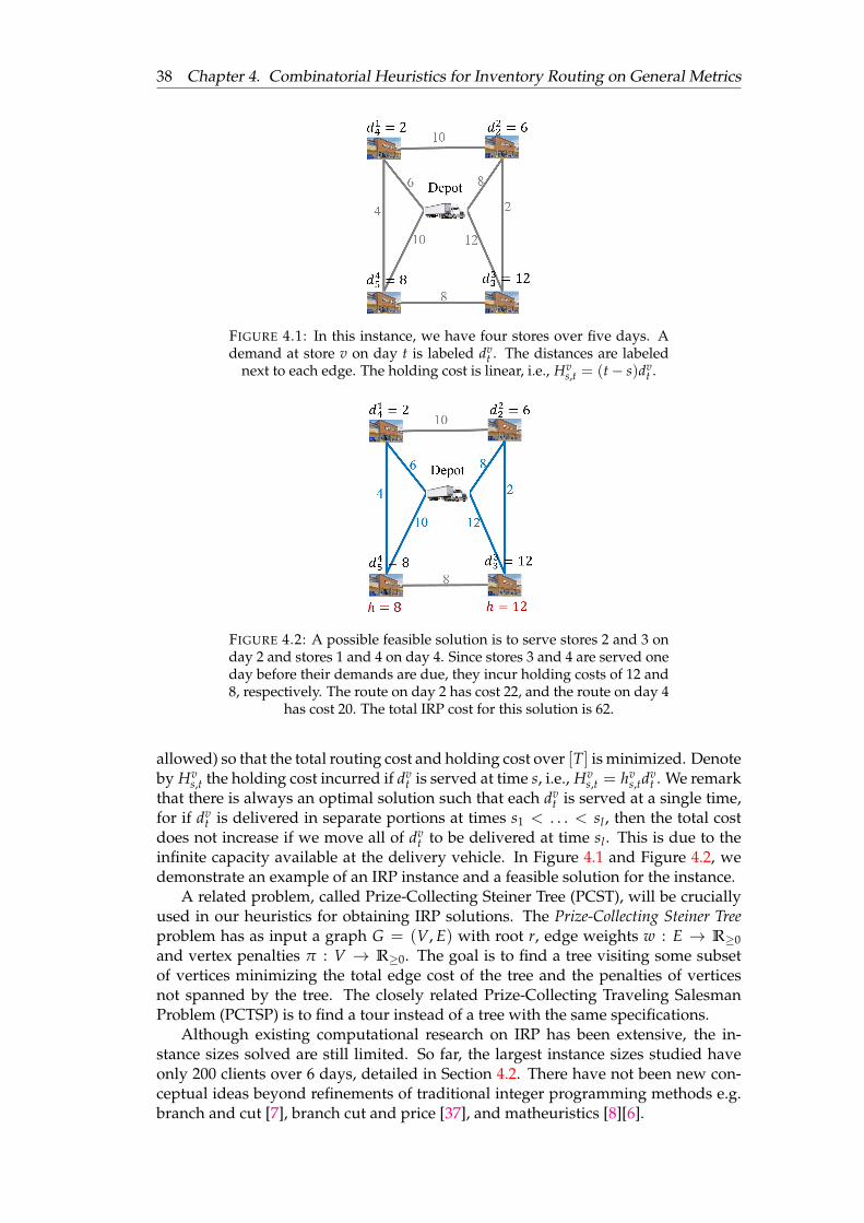
38 Chapter 4. Combinatorial Heuristics for Inventory Routing on General Metrics

FIGURE 4.1: In this instance, we have four stores over five days. Ademand at store v on day t is labeled dv

t . The distances are labelednext to each edge. The holding cost is linear, i.e., Hv

s,t = (t− s)dvt .

FIGURE 4.2: A possible feasible solution is to serve stores 2 and 3 onday 2 and stores 1 and 4 on day 4. Since stores 3 and 4 are served oneday before their demands are due, they incur holding costs of 12 and8, respectively. The route on day 2 has cost 22, and the route on day 4

has cost 20. The total IRP cost for this solution is 62.

allowed) so that the total routing cost and holding cost over [T] is minimized. Denoteby Hv

s,t the holding cost incurred if dvt is served at time s, i.e., Hv

s,t = hvs,td

vt . We remark

that there is always an optimal solution such that each dvt is served at a single time,

for if dvt is delivered in separate portions at times s1 < . . . < sl , then the total cost

does not increase if we move all of dvt to be delivered at time sl . This is due to the

infinite capacity available at the delivery vehicle. In Figure 4.1 and Figure 4.2, wedemonstrate an example of an IRP instance and a feasible solution for the instance.

A related problem, called Prize-Collecting Steiner Tree (PCST), will be cruciallyused in our heuristics for obtaining IRP solutions. The Prize-Collecting Steiner Treeproblem has as input a graph G = (V, E) with root r, edge weights w : E → R≥0and vertex penalties π : V → R≥0. The goal is to find a tree visiting some subsetof vertices minimizing the total edge cost of the tree and the penalties of verticesnot spanned by the tree. The closely related Prize-Collecting Traveling SalesmanProblem (PCTSP) is to find a tour instead of a tree with the same specifications.

Although existing computational research on IRP has been extensive, the in-stance sizes solved are still limited. So far, the largest instance sizes studied haveonly 200 clients over 6 days, detailed in Section 4.2. There have not been new con-ceptual ideas beyond refinements of traditional integer programming methods e.g.branch and cut [7], branch cut and price [37], and matheuristics [8][6].

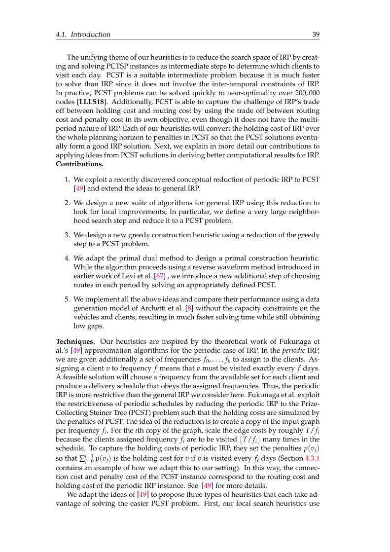
4.1. Introduction 39

The unifying theme of our heuristics is to reduce the search space of IRP by creat-ing and solving PCTSP instances as intermediate steps to determine which clients tovisit each day. PCST is a suitable intermediate problem because it is much fasterto solve than IRP since it does not involve the inter-temporal constraints of IRP.In practice, PCST problems can be solved quickly to near-optimality over 200, 000nodes [LLLS18]. Additionally, PCST is able to capture the challenge of IRP’s tradeoff between holding cost and routing cost by using the trade off between routingcost and penalty cost in its own objective, even though it does not have the multi-period nature of IRP. Each of our heuristics will convert the holding cost of IRP overthe whole planning horizon to penalties in PCST so that the PCST solutions eventu-ally form a good IRP solution. Next, we explain in more detail our contributions toapplying ideas from PCST solutions in deriving better computational results for IRP.Contributions.

1. We exploit a recently discovered conceptual reduction of periodic IRP to PCST[49] and extend the ideas to general IRP.

2. We design a new suite of algorithms for general IRP using this reduction tolook for local improvements; In particular, we define a very large neighbor-hood search step and reduce it to a PCST problem.

3. We design a new greedy construction heuristic using a reduction of the greedystep to a PCST problem.

4. We adapt the primal dual method to design a primal construction heuristic.While the algorithm proceeds using a reverse waveform method introduced inearlier work of Levi et al. [67] , we introduce a new additional step of choosingroutes in each period by solving an appropriately defined PCST.

5. We implement all the above ideas and compare their performance using a datageneration model of Archetti et al. [8] without the capacity constraints on thevehicles and clients, resulting in much faster solving time while still obtaininglow gaps.

Techniques. Our heuristics are inspired by the theoretical work of Fukunaga etal.’s [49] approximation algorithms for the periodic case of IRP. In the periodic IRP,we are given additionally a set of frequencies f0, . . . , fk to assign to the clients. As-signing a client v to frequency f means that v must be visited exactly every f days.A feasible solution will choose a frequency from the available set for each client andproduce a delivery schedule that obeys the assigned frequencies. Thus, the periodicIRP is more restrictive than the general IRP we consider here. Fukunaga et al. exploitthe restrictiveness of periodic schedules by reducing the periodic IRP to the Prize-Collecting Steiner Tree (PCST) problem such that the holding costs are simulated bythe penalties of PCST. The idea of the reduction is to create a copy of the input graphper frequency fi. For the ith copy of the graph, scale the edge costs by roughly T/ fibecause the clients assigned frequency fi are to be visited bT/ fic many times in theschedule. To capture the holding costs of periodic IRP, they set the penalties p(vj)

so that ∑i−1j=0 p(vj) is the holding cost for v if v is visited every fi days (Section 4.3.1

contains an example of how we adapt this to our setting). In this way, the connec-tion cost and penalty cost of the PCST instance correspond to the routing cost andholding cost of the periodic IRP instance. See [49] for more details.

We adapt the ideas of [49] to propose three types of heuristics that each take ad-vantage of solving the easier PCST problem. First, our local search heuristics use

40 Chapter 4. Combinatorial Heuristics for Inventory Routing on General Metrics

PCST to quickly perform large neighborhood search among the potential improve-ments per round. Adaptive large neighborhood search has been used on IRP withTransshipments [CCL12a] and Multi-vehicle IRP [CCL12b]. Large neighborhoodsearch has also been investigated on other variants of IRP [81, 2, 54].

Second, our greedy heuristic uses PCST to determine the best density demandset to cover each round. Finally, the primal-dual heuristic uses PCST to guide thegrowth of the dual values and identify the set of demands to serve. We describethe motivation for using PCSTs in Section 4.3. The best of our heuristics achievesoptimality ratios between 1.04 and 1.08 (across various problem settings), and yetwas able to solve instances of size 140 clients over 6 days and 50 clients over 14 dayswithin 2.01 seconds and under 1 second, respectively. They are still able to solveeven larger instances quickly, but we do not have lower bounds to evaluate theirsolution quality for instances larger than the aforementioned sizes. Both of thesesolution times are over three orders of magnitude faster than solving a single com-modity flow MIP model of IRP, which requires over 2837 seconds and 1481 seconds,respectively, to solve within 10% MIPGap.Chapter Outline. The remaining sections are organized as follows. In Section 4.2,we describe related work. Section 4.3 describes three local search heuristics. Sec-tion 4.4 provides a greedy heuristic. Section 4.5 presents a primal dual heuristic. InSection 4.6, we describe a single commodity flow MIP formulation of IRP to attainlower bounds for the costs of optimal solutions to compare with the heuristics. Fi-nally, Section 4.7 shows the computational results of the various heuristics across arange of input parameters.

4.2 Related Work

Methods for Capacitated IRP. For the capacitated single-vehicle deterministic IRP,Archetti et al. [7] introduced and found exact solutions for small benchmark instancesof up to 50 clients over 3 days and up to 30 clients over 6 days. Later, Archettiet al. [8] gave a heuristic combining tabu search with MIPs that found near-optimalsolutions to the small instances. They also improved upper bounds on large instancesof 200 clients over 6 days in the case of order-up-to-level policy. For the more generalmultivehicle case, Desaulniers et al. [37] provide a branch-price-and-cut algorithm,finding 54 new optima out of the 238 instances from Archetti et al. [8] with unknownoptima. Archetti et al. [6] give a metaheuristic that solves MIPs both before andafter tabu search. To initialize a solution, they formulate MIPs of different strengthsand choose the MIP based on the instance size, stronger MIP for smaller instances.Then the tabu search adds, deletes, or moves visits. If the instance was small, theMIP after the tabu search fixes some variables to integer values based on how oftenthe variable is 0 or 1 among the solutions from the search. For large instances, theroutes from the tabu solutions are included as route variables in the MIP. They wereable to improve the upper bound on 224 of the 240 large instances. We remark thatour results are not directly comparable with these existing results since we considerthe uncapacitated version of the problem. To the best of our knowledge, there are nocomputational studies specifically geared towards the uncapacitated IRP consideredhere. However, as a starting point, we test our heuristics on uncapacitated instanceshaving the same parameter values (except for the capacities that we ignore) as thelarge instances of size 200 by 6 [8].Prize-Collecting Steiner Trees and Tours. Since we will use the solvers for PCSTin our implementation, we also review previous work on PCST. Specifically, we use

4.3. Local Search 41

the dual-ascent-based branch-and-bound solver of Leitner et al. [LLLS18] for PCST,which reaches near-optimality and performs the fastest on many categories of in-stances from the DIMACS Challenge. Prior to this, Ljubic et al. [71] and Fischetti etal. [46] provided the most competitive algorithms to find exact solutions for PCST.Whenever we obtain a tree from the solver [LLLS18], we convert the tree to a tourby running the TSP solver Concorde [Cook15] on the subset of vertices spanned bythe tree.

Theoretically, our greedy algorithm will solve a PCST problem to find low den-sity set covers. The solution to each PCST instance will come from the primal dualalgorithm for PCST [55], whose analysis is used in eventually proving a logarithmicfactor guarantee of our greedy algorithm for IRP.Approximation Algorithms for IRP. On the theoretical side, approximation algo-rithms for special cases of IRP have been studied but mostly for the uncapacitatedversions that we study here. IRP on general metrics has a O( log T

log log T )-approximationby Nagarajan and Shi [73] and an O(log N)-approximation by Fukunaga et al [49].For variants of periodic IRP, Fukunaga et al. [49] provide constant approximations.Another special case of IRP is the joint replenishment problem (JRP). JRP is equiv-alent to IRP on a two-level tree metric, where the first level has one edge of costK0 and the second level consists of children of the first level, with an edge of costKi for each commodity i. JRP is known to be NP-hard [9] and APX-hard [75]. Onthe positive side, Levi et al. [67] give a 2-approximation via a primal dual approach.The approximation factor was reduced to 1.8 in [68] by LP rounding. Bienkowski etal. [17] improve the approximation factor further to 1.791 by randomized rounding.

4.3 Local Search

We examine three local search algorithms: DELETE, ADD, and prioritized.Among them, the latter two solve PCSTs to compute the improvement step. Thereason we use PCST in our heuristics is that solving PCSTs allows us to attain locallyoptimal solutions to IRP. In the ADD local search, an ADD operation on day s willfind the subset of clients whose addition to the existing visit set on day s maximizesthe total cost savings from the current solution. This best subset is found by solvinga PCST problem with appropriately constructed penalties that capture the savings inholding cost for extra visits. The extra connection cost is naturally modeled into theedge costs of the PCST problem. To keep track of the feasible solutions found duringthe local searches, we use T to denote candidate solutions to the IRP, overloading itwith all the relevant information in the solution such as the trees in the daily visits,the visit times at each demand and the implied holding costs. Since global optimal-ity implies local optimality, if we started with an optimal solution T and deleted allvisits on a fixed day, then applying ADD on that day will yield back the original setvisited by T.

We prove this claim formally in Lemma 4.3.1 of Section 4.3.2.All of the local searches rely on the fact that the test instances generated using

Archetti et al.’s model have all positive demands for every v ∈ V, 1 ≤ t ≤ T. So alllocal search heuristics consider modifying the visit set only on days 2, . . . , T, not day1, since any feasible solution must satisfy all the demands on day 1.

To obtain an IRP solution at the end, we convert each day’s tree into a tour vis-iting the clients spanned by the tree by calling Concorde on the graph induced bythe spanned clients. We will apply the same conversion from trees to tours in allremaining heuristics as well.

42 Chapter 4. Combinatorial Heuristics for Inventory Routing on General Metrics

In Section 4.3.1, we introduce a local search procedure that applies onlyDELETEs. Section 4.3.2 describes a local search procedure applying only ADDs.In Section 4.3.3 we introduce the DELETE-ADD operation and define a more refinedlocal search that applies all three operations in order of complexity.

4.3.1 DELETE

In the delete-only local search, we start with a feasible solution that visits every-one everyday and delete an entire day’s visit as long as it makes an improvement.

We define the following notations needed for the algorithm. Let l(v, s) be thelatest visit before day s that visits v. Denote by Ts the existing tree on day s in thecurrent step of the algorithm. We use the vector T to represent the current set ofexisting trees on each day throughout the time horizon. Let t(v, s) be the latest day tsuch T does not visit v during the time interval [s + 1, t]. Notice that if a visit to v onday s is removed, then each demand (v, t) with t ∈ [s, t(v, s)] would incur an extraholding cost of Hv

l(v,s),t − Hvs,t. So we set the penalty of removing v on day s to be

πs(v) :=

∑t(v,s)

t=s (Hvl(v,s),t − Hv

s,t) if v ∈ Ts

0 else.(4.1)

If the tree Ts on day s is deleted, then the routing cost decreases by c(E(Ts)) andthe change to the holding cost increases by πs(V(Ts)). So the total change in costfor deleting the tree on day s is ∆DELETE(s) := −c(E(Ts)) + πs(V(Ts)). Finally, theoperation DELETE(s) removes the existing tree Ts on day s.

Denote by c(T) the total cost of a solution T. The improvement ratio of an operationis the magnitude of the change in cost induced by the operation divided by the totalcost of the current feasible solution. In all of the local search heuristics, whenever wescan through the time period to find an improving step, we will make the improvingoperation on the day that gives the best improvement. To avoid potentially longrunning time, we shall stop looking for improvements whenever the best possibleimprovement ratio is smaller than some small value, typically 0.01.

Now, we formally define the DELETE algorithm.

Algorithm 1 Local Search with DELETE

1: Initialize a feasible solution T.2: Let t′ = arg mins∈[2,T] ∆DELETE(s).

3: while |∆DELETE(t′)||c(T)| ≥ 0.01 do

4: DELETE(t′)5: end while

The initial feasible solution here is a “full” solution, where each day consists ofa minimum cost tree that visits everyone. We delete only trees within time [2, T]to keep the solution feasible. Since all (v, t) have positive demands, any feasiblesolution must visit everyone on day 1. So leaving T1 untouched does not make oursolution costlier than a local optimum.

4.3.2 ADD

In the add-only local search, we start with a feasible solution and we find anoptimal subset of clients to add to the current subset on some day as long as it im-proves the total cost. To find the best subset of clients to add on a given day s, we

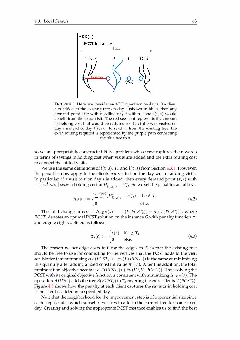
4.3. Local Search 43

FIGURE 4.3: Here, we consider an ADD operation on day s. If a clientv is added to the existing tree on day s (shown in blue), then anydemand point at v with deadline day t within s and t(v, s) wouldbenefit from the extra visit. The red segment represents the amountof holding cost that would be reduced for (v, t) if v was visited onday s instead of day l(v, s). To reach v from the existing tree, theextra routing required is represented by the purple path connecting

the blue tree to v.

solve an appropriately constructed PCST problem whose cost captures the rewardsin terms of savings in holding cost when visits are added and the extra routing costto connect the added visits.

We use the same definitions of l(v, s), Ts, and t(v, s) from Section 4.3.1. However,the penalties now apply to the clients not visited on the day we are adding visits.In particular, if a visit to v on day s is added, then every demand point (v, t) witht ∈ [s, t(s, v)] saves a holding cost of Hv

l(v,s),t− Hvs,t. So we set the penalties as follows.

πs(v) :=

∑t(v,s)

t=s (Hvl(v,s),t − Hv

s,t) if v /∈ Ts

0 else.(4.2)

The total change in cost is ∆ADD(s) := c(E(PCSTs)) − πs(V(PCSTs)), wherePCSTs denotes an optimal PCST solution on the instance G with penalty function πsand edge weights defined as follows.

ws(e) :=

c(e) if e /∈ Ts

0 else.(4.3)

The reason we set edge costs to 0 for the edges in Ts is that the existing treeshould be free to use for connecting to the vertices that the PCST adds to the visitset. Notice that minimizing c(E(PCSTs))−πs(V(PCSTs)) is the same as minimizingthis quantity after adding a fixed constant value πs(V). After this addition, the totalminimization objective becomes c(E(PCSTs))+πs(V \V(PCSTs)). Thus solving thePCST with its original objective function is consistent with minimizing ∆ADD(s). Theoperation ADD(s) adds the tree E(PCSTs) to Ts covering the extra clients V(PCSTs).Figure 4.3 shows how the penalty at each client captures the savings in holding costif the client is added on a specified day.

Note that the neighborhood for the improvement step is of exponential size sinceeach step decides which subset of vertices to add to the current tree for some fixedday. Creating and solving the appropriate PCST instance enables us to find the best

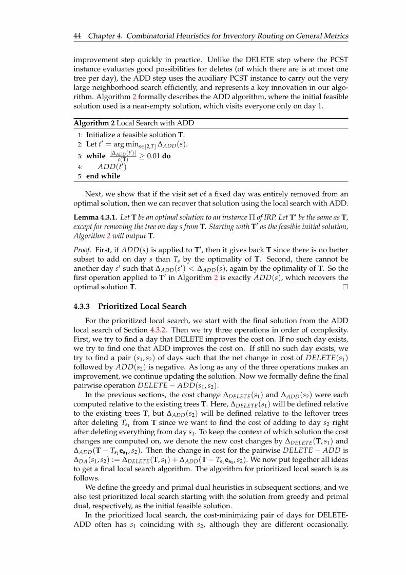
44 Chapter 4. Combinatorial Heuristics for Inventory Routing on General Metrics

improvement step quickly in practice. Unlike the DELETE step where the PCSTinstance evaluates good possibilities for deletes (of which there are is at most onetree per day), the ADD step uses the auxiliary PCST instance to carry out the verylarge neighborhood search efficiently, and represents a key innovation in our algo-rithm. Algorithm 2 formally describes the ADD algorithm, where the initial feasiblesolution used is a near-empty solution, which visits everyone only on day 1.

Algorithm 2 Local Search with ADD

1: Initialize a feasible solution T.2: Let t′ = arg mins∈[2,T] ∆ADD(s).

3: while |∆ADD(t′)|c(T) ≥ 0.01 do

4: ADD(t′)5: end while

Next, we show that if the visit set of a fixed day was entirely removed from anoptimal solution, then we can recover that solution using the local search with ADD.

Lemma 4.3.1. Let T be an optimal solution to an instance Π of IRP. Let T′ be the same as T,except for removing the tree on day s from T. Starting with T′ as the feasible initial solution,Algorithm 2 will output T.

Proof. First, if ADD(s) is applied to T′, then it gives back T since there is no bettersubset to add on day s than Ts by the optimality of T. Second, there cannot beanother day s′ such that ∆ADD(s′) < ∆ADD(s), again by the optimality of T. So thefirst operation applied to T′ in Algorithm 2 is exactly ADD(s), which recovers theoptimal solution T.

4.3.3 Prioritized Local Search

For the prioritized local search, we start with the final solution from the ADDlocal search of Section 4.3.2. Then we try three operations in order of complexity.First, we try to find a day that DELETE improves the cost on. If no such day exists,we try to find one that ADD improves the cost on. If still no such day exists, wetry to find a pair (s1, s2) of days such that the net change in cost of DELETE(s1)followed by ADD(s2) is negative. As long as any of the three operations makes animprovement, we continue updating the solution. Now we formally define the finalpairwise operation DELETE− ADD(s1, s2).

In the previous sections, the cost change ∆DELETE(s1) and ∆ADD(s2) were eachcomputed relative to the existing trees T. Here, ∆DELETE(s1) will be defined relativeto the existing trees T, but ∆ADD(s2) will be defined relative to the leftover treesafter deleting Ts1 from T since we want to find the cost of adding to day s2 rightafter deleting everything from day s1. To keep the context of which solution the costchanges are computed on, we denote the new cost changes by ∆DELETE(T, s1) and∆ADD(T− Ts1es1 , s2). Then the change in cost for the pairwise DELETE− ADD is∆DA(s1, s2) := ∆DELETE(T, s1) + ∆ADD(T− Ts1es1 , s2). We now put together all ideasto get a final local search algorithm. The algorithm for prioritized local search is asfollows.

We define the greedy and primal dual heuristics in subsequent sections, and wealso test prioritized local search starting with the solution from greedy and primaldual, respectively, as the initial feasible solution.

In the prioritized local search, the cost-minimizing pair of days for DELETE-ADD often has s1 coinciding with s2, although they are different occasionally.

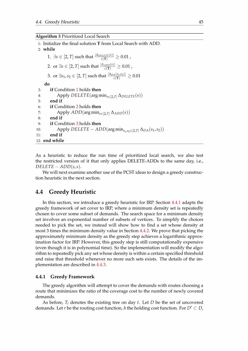
4.4. Greedy Heuristic 45

Algorithm 3 Prioritized Local Search

1: Initialize the final solution T from Local Search with ADD.2: while

1. ∃s ∈ [2, T] such that |∆DELETE(s)|c(T) ≥ 0.01 ,

2. or ∃s ∈ [2, T] such that |∆ADD(s)|c(T) ≥ 0.01 ,

3. or ∃s1, s2 ∈ [2, T] such that |∆DA(s1,s2)|c(T) ≥ 0.01

do3: if Condition 1 holds then4: Apply DELETE(arg mins∈[2,T] ∆DELETE(s))5: end if6: if Condition 2 holds then7: Apply ADD(arg mins∈[2,T] ∆ADD(s))8: end if9: if Condition 3 holds then

10: Apply DELETE− ADD(arg mins1,s2∈[2,T] ∆DA(s1, s2))11: end if12: end while

As a heuristic to reduce the run time of prioritized local search, we also testthe restricted version of it that only applies DELETE-ADDs to the same day, i.e.,DELETE− ADD(s, s).

We will next examine another use of the PCST ideas to design a greedy construc-tion heuristic in the next section.

4.4 Greedy Heuristic

In this section, we introduce a greedy heuristic for IRP. Section 4.4.1 adapts thegreedy framework of set cover to IRP, where a minimum density set is repeatedlychosen to cover some subset of demands. The search space for a minimum densityset involves an exponential number of subsets of vertices. To simplify the choicesneeded to pick the set, we instead will show how to find a set whose density atmost 3 times the minimum density value in Section 4.4.2. We prove that picking theapproximately minimum density as the greedy step achieves a logarithmic approx-imation factor for IRP. However, this greedy step is still computationally expensive(even though it is in polynomial time). So the implementation will modify the algo-rithm to repeatedly pick any set whose density is within a certain specified thresholdand raise that threshold whenever no more such sets exists. The details of the im-plementation are described in 4.4.3.

4.4.1 Greedy Framework

The greedy algorithm will attempt to cover the demands with routes choosing aroute that minimizes the ratio of the coverage cost to the number of newly covereddemands.

As before, Tt denotes the existing tree on day t. Let D be the set of uncovereddemands. Let r be the routing cost function, h the holding cost function. For D′ ⊂ D,

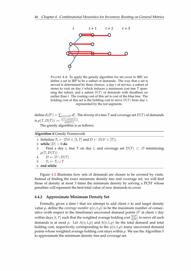
46 Chapter 4. Combinatorial Heuristics for Inventory Routing on General Metrics

FIGURE 4.4: To apply the greedy algorithm for set cover to IRP, wedefine a set in IRP to be a subset of demands. The way that a set isserved is determined by three choices: a day t of service, a subset ofstores to visit on day t which induces a minimum cost tree T span-ning the subset, and a subset D(T) of demands with deadlines noearlier than t. The routing cost of this set is cost of the blue tree. Theholding cost of this set is the holding cost to serve D(T) from day t,

represented by the red segments.

define d(D′) = ∑(v,t)∈D′ dvt . The density of a tree T and coverage set D(T) of demands

is ρ(T, D(T)) := r(T)+h(D(T))d(D(T)) .

The greedy algorithm is as follows.

Algorithm 4 Greedy Framework

1: Initialize Tt ← ∅∀t ∈ [1, T] and D ← D(V × [T]).2: while |D| > 0 do3: Find a day t, tree T on day t, and coverage set D(T) ⊂ D minimizing

ρ(T, D(T))4: D ← D \ D(T)5: Tt ← Tt ∪ T6: end while

Figure 4.4 illustrates how sets of demands are chosen to be covered by visits.Instead of finding the exact minimum density tree and coverage set, we will findthose of density at most 3 times the minimum density by solving a PCST whosepenalties will represent the best total value of new demands to cover.

4.4.2 Approximate Minimum Density Set

Formally, given a time t that we attempt to add client v to and target densityvalue ρ, define the coverage number η(v, t, ρ) to be the maximum number of consec-utive (with respect to the timeframe) uncovered demand points D′ at client v daywithin days [t, T] such that the weighted average holding cost h(D′)

d(D′) to serve all suchdemands is at most ρ. Let A(v, t, ρ) and h(v, t, ρ) be the total demand and totalholding cost, respectively, corresponding to the η(v, t, ρ) many uncovered demandpoints whose weighted average holding cost stays within ρ. We use the Algorithm 0to approximate the minimum density tree and coverage set.

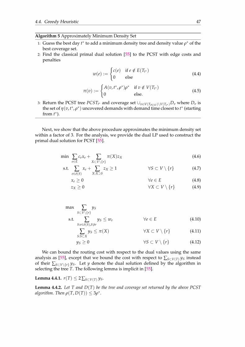
4.4. Greedy Heuristic 47

Algorithm 5 Approximately Minimum Density Set

1: Guess the best day t∗ to add a minimum density tree and density value ρ∗ of thebest coverage set.

2: Find the classical primal dual solution [55] to the PCST with edge costs andpenalties

w(e) :=

c(e) if e /∈ E(Tt∗)

0 else(4.4)

π(v) :=

A(v, t∗, ρ∗)ρ∗ if v /∈ V(Tt∗)

0 else.(4.5)

3: Return the PCST tree PCSTt∗ and coverage set ∪v∈V(TPCST)\V(Tt∗ )Dv where Dv is

the set of η(v, t∗, ρ∗) uncovered demands with demand time closest to t∗ (startingfrom t∗).

Next, we show that the above procedure approximates the minimum density setwithin a factor of 3. For the analysis, we provide the dual LP used to construct theprimal dual solution for PCST [55].

min ∑e∈E

cexe + ∑X⊂V\r

π(X)zX (4.6)

s.t. ∑e∈δ(S)

xe + ∑X:X⊃S

zX ≥ 1 ∀S ⊂ V \ r (4.7)

xe ≥ 0 ∀e ∈ E (4.8)zX ≥ 0 ∀X ⊂ V \ r (4.9)

max ∑S⊂V\r

yS

s.t. ∑S:e∈δ(S),S 63r

yS ≤ we ∀e ∈ E (4.10)

∑S:S⊂X

yS ≤ π(X) ∀X ⊂ V \ r (4.11)

yS ≥ 0 ∀S ⊂ V \ r (4.12)

We can bound the routing cost with respect to the dual values using the sameanalysis as [55], except that we bound the cost with respect to ∑S⊂V(T) yS insteadof their ∑S⊂V\r yS. Let y denote the dual solution defined by the algorithm inselecting the tree T. The following lemma is implicit in [55].

Lemma 4.4.1. r(T) ≤ 2 ∑S⊂V(T) yS.

Lemma 4.4.2. Let T and D(T) be the tree and coverage set returned by the above PCSTalgorithm. Then ρ(T, D(T)) ≤ 3ρ∗.

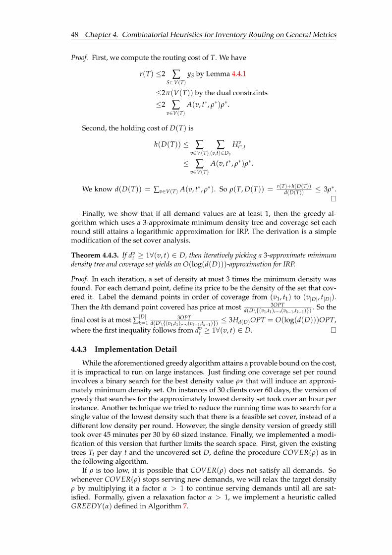
48 Chapter 4. Combinatorial Heuristics for Inventory Routing on General Metrics

Proof. First, we compute the routing cost of T. We have

r(T) ≤2 ∑S⊂V(T)

yS by Lemma 4.4.1

≤2π(V(T)) by the dual constraints

≤2 ∑v∈V(T)

A(v, t∗, ρ∗)ρ∗.

Second, the holding cost of D(T) is

h(D(T)) ≤ ∑v∈V(T)

∑(v,t)∈Dv

Hvt∗,t

≤ ∑v∈V(T)

A(v, t∗, ρ∗)ρ∗.

We know d(D(T)) = ∑v∈V(T) A(v, t∗, ρ∗). So ρ(T, D(T)) = r(T)+h(D(T))d(D(T)) ≤ 3ρ∗.

Finally, we show that if all demand values are at least 1, then the greedy al-gorithm which uses a 3-approximate minimum density tree and coverage set eachround still attains a logarithmic approximation for IRP. The derivation is a simplemodification of the set cover analysis.

Theorem 4.4.3. If dvt ≥ 1∀(v, t) ∈ D, then iteratively picking a 3-approximate minimum

density tree and coverage set yields an O(log(d(D)))-approximation for IRP.

Proof. In each iteration, a set of density at most 3 times the minimum density wasfound. For each demand point, define its price to be the density of the set that cov-ered it. Label the demand points in order of coverage from (v1, t1) to (v|D|, t|D|).Then the kth demand point covered has price at most 3OPT

d(D\(v1,t1),...,(vk−1,tk−1)). So the

final cost is at most ∑|D|k=13OPT

d(D\(v1,t1),...,(vk−1,tk−1))≤ 3Hd(D)OPT = O(log(d(D)))OPT,

where the first inequality follows from dvt ≥ 1∀(v, t) ∈ D.

4.4.3 Implementation Detail

While the aforementioned greedy algorithm attains a provable bound on the cost,it is impractical to run on large instances. Just finding one coverage set per roundinvolves a binary search for the best density value ρ∗ that will induce an approxi-mately minimum density set. On instances of 30 clients over 60 days, the version ofgreedy that searches for the approximately lowest density set took over an hour perinstance. Another technique we tried to reduce the running time was to search for asingle value of the lowest density such that there is a feasible set cover, instead of adifferent low density per round. However, the single density version of greedy stilltook over 45 minutes per 30 by 60 sized instance. Finally, we implemented a modi-fication of this version that further limits the search space. First, given the existingtrees Tt per day t and the uncovered set D, define the procedure COVER(ρ) as inthe following algorithm.

If ρ is too low, it is possible that COVER(ρ) does not satisfy all demands. Sowhenever COVER(ρ) stops serving new demands, we will relax the target densityρ by multiplying it a factor α > 1 to continue serving demands until all are sat-isfied. Formally, given a relaxation factor α > 1, we implement a heuristic calledGREEDY(α) defined in Algorithm 7.

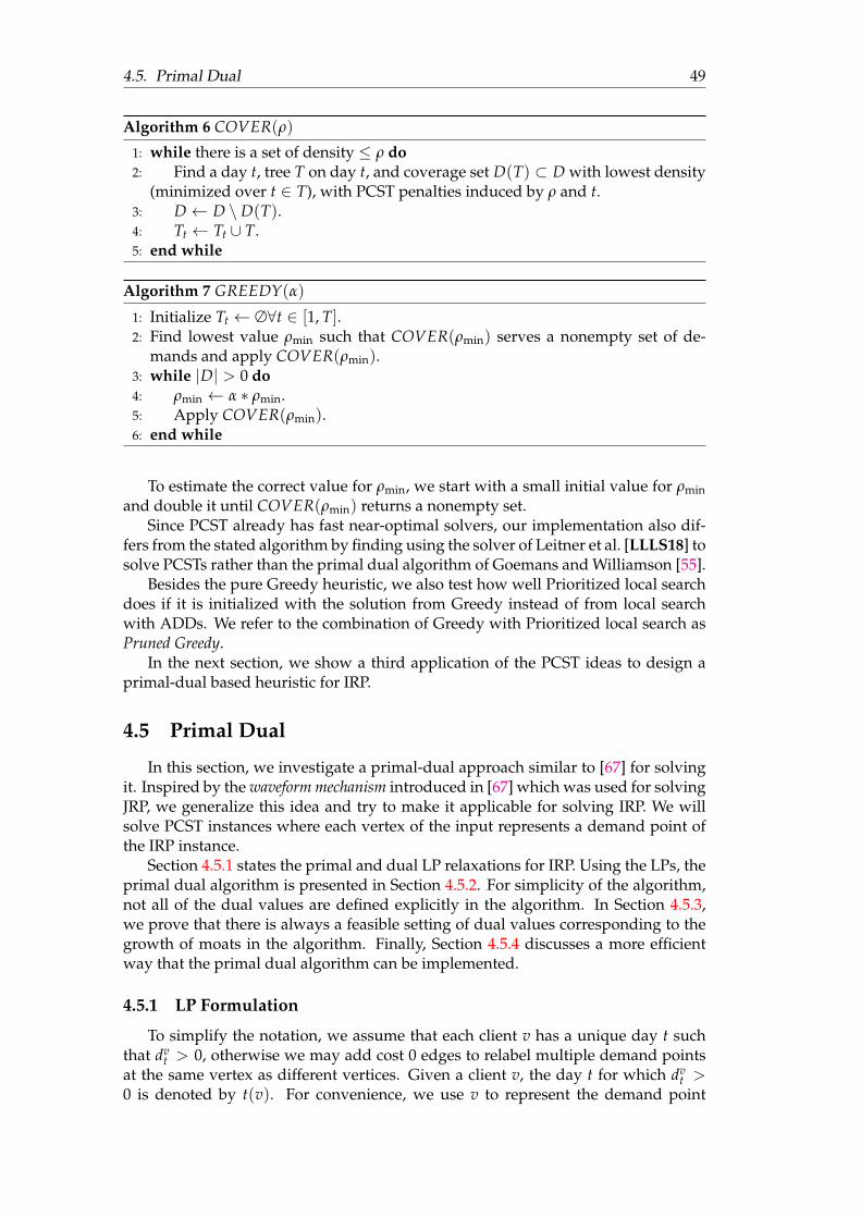
4.5. Primal Dual 49

Algorithm 6 COVER(ρ)

1: while there is a set of density ≤ ρ do2: Find a day t, tree T on day t, and coverage set D(T) ⊂ D with lowest density

(minimized over t ∈ T), with PCST penalties induced by ρ and t.3: D ← D \ D(T).4: Tt ← Tt ∪ T.5: end while

Algorithm 7 GREEDY(α)

1: Initialize Tt ← ∅∀t ∈ [1, T].2: Find lowest value ρmin such that COVER(ρmin) serves a nonempty set of de-

mands and apply COVER(ρmin).3: while |D| > 0 do4: ρmin ← α ∗ ρmin.5: Apply COVER(ρmin).6: end while

To estimate the correct value for ρmin, we start with a small initial value for ρminand double it until COVER(ρmin) returns a nonempty set.

Since PCST already has fast near-optimal solvers, our implementation also dif-fers from the stated algorithm by finding using the solver of Leitner et al. [LLLS18] tosolve PCSTs rather than the primal dual algorithm of Goemans and Williamson [55].

Besides the pure Greedy heuristic, we also test how well Prioritized local searchdoes if it is initialized with the solution from Greedy instead of from local searchwith ADDs. We refer to the combination of Greedy with Prioritized local search asPruned Greedy.

In the next section, we show a third application of the PCST ideas to design aprimal-dual based heuristic for IRP.

4.5 Primal Dual

In this section, we investigate a primal-dual approach similar to [67] for solvingit. Inspired by the waveform mechanism introduced in [67] which was used for solvingJRP, we generalize this idea and try to make it applicable for solving IRP. We willsolve PCST instances where each vertex of the input represents a demand point ofthe IRP instance.

Section 4.5.1 states the primal and dual LP relaxations for IRP. Using the LPs, theprimal dual algorithm is presented in Section 4.5.2. For simplicity of the algorithm,not all of the dual values are defined explicitly in the algorithm. In Section 4.5.3,we prove that there is always a feasible setting of dual values corresponding to thegrowth of moats in the algorithm. Finally, Section 4.5.4 discusses a more efficientway that the primal dual algorithm can be implemented.

4.5.1 LP Formulation

To simplify the notation, we assume that each client v has a unique day t suchthat dv

t > 0, otherwise we may add cost 0 edges to relabel multiple demand pointsat the same vertex as different vertices. Given a client v, the day t for which dv

t >0 is denoted by t(v). For convenience, we use v to represent the demand point

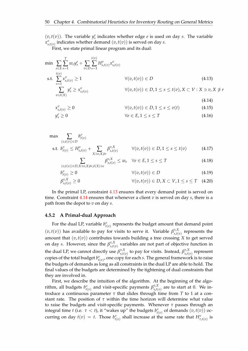
50 Chapter 4. Combinatorial Heuristics for Inventory Routing on General Metrics

(v, t(v)). The variable yes indicates whether edge e is used on day s. The variable

xvs,t(v) indicates whether demand (v, t(v)) is served on day s.

First, we state primal linear program and its dual:

min ∑e∈E

T

∑s=1

weyes + ∑

v∈D

t(v)

∑s=1

Hvs,t(v)x

vs,t(v)

s.t.t(v)

∑s=1

xvs,t(v) ≥ 1 ∀(v, t(v)) ∈ D (4.13)

∑e∈δ(X)

yes ≥ xv

s,t(v) ∀(v, t(v)) ∈ D, 1 ≤ s ≤ t(v), X ⊂ V : X 3 v, X 63 r

(4.14)

xvs,t(v) ≥ 0 ∀(v, t(v)) ∈ D, 1 ≤ s ≤ v(t) (4.15)

yes ≥ 0 ∀e ∈ E, 1 ≤ s ≤ T (4.16)

max ∑(v,t(v))∈D

bvt(v)

s.t. bvt(v) ≤ Hv

s,t(v) + ∑X3v,X 63r

βv,Xs,t(v) ∀(v, t(v)) ∈ D, 1 ≤ s ≤ t(v) (4.17)

∑(v,t(v))∈D,X3v,X 63r,δ(X)3e

βv,Xs,t(v) ≤ we ∀e ∈ E, 1 ≤ s ≤ T (4.18)

bvt(v) ≥ 0 ∀(v, t(v)) ∈ D (4.19)

βv,Xs,t(v) ≥ 0 ∀(v, t(v)) ∈ D, X ⊂ V, 1 ≤ s ≤ T (4.20)

In the primal LP, constraint 4.13 ensures that every demand point is served ontime. Constraint 4.14 ensures that whenever a client v is served on day s, there is apath from the depot to v on day s.

4.5.2 A Primal-dual Approach

For the dual LP, variable bvt(v) represents the budget amount that demand point

(v, t(v)) has available to pay for visits to serve it. Variable βv,Xs,t(v) represents the

amount that (v, t(v)) contributes towards building a tree crossing X to get servedon day s. However, since the βv,X

s,t(v) variables are not part of objective function in

the dual LP, we cannot directly use βv,Xs,t(v) to pay for visits. Instead, βv,X

s,t(v) representcopies of the total budget bv

t(v), one copy for each s. The general framework is to raisethe budgets of demands as long as all constraints in the dual LP are able to hold. Thefinal values of the budgets are determined by the tightening of dual constraints thatthey are involved in.

First, we describe the intuition of the algorithm. At the beginning of the algo-rithm, all budgets bv

t(v) and visit-specific payments βv,Xs,t(v) are to start at 0. We in-

troduce a continuous parameter τ that slides through time from T to 1 at a con-stant rate. The position of τ within the time horizon will determine what valueto raise the budgets and visit-specific payments. Whenever τ passes through anintegral time t (i.e. τ < t), it “wakes up” the budgets bv

t(v) of demands (v, t(v)) oc-curring on day t(v) = t. Those bv

t(v) shall increase at the same rate that Hvτ,t(v) is

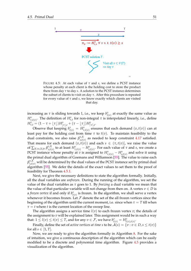
4.5. Primal Dual 51

FIGURE 4.5: At each value of τ and s, we define a PCST instancewhose penalty at each client is the holding cost to store the productthere from day τ to day s. A solution to the PCST instance determinesthe subset of clients to visit on day τ. After this procedure is repeatedfor every value of τ and s, we know exactly which clients are visited

that day.

increasing as τ is sliding towards 1, i.e., we keep bvt(v) at exactly the same value as

Hvτ,t(v). The definition of Hv

τ,t for non-integral τ is interpolated linearly, i.e., defineHv

τ,t = (1− τ + bτc)Hvbτc,t + (τ − bτc)Hv

dτe,t.Observe that keeping bv

t(v) = Hvτ,t(v) ensures that each demand (v, t(v)) can at

least pay for the holding cost from time τ to t(v). To maintain feasibility to thedual constraints, we also raise βv,X

s,t(v) as needed to keep constraint 4.17 satisfied.That means for each demand (v, t(v)) and each s ∈ (τ, t(v)], we raise the valueof ∑X3v,X 63r βv,X

s,t(v) to at least Hvτ,t(v) − Hv

s,t(v). For each value of τ and s, we create aPCST instance whose penalty at v is assigned to Hv

τ,t(v) − Hvs,t(v) and solve it using

the primal dual algorithm of Goemans and Williamson [55]. The value to raise eachβv,X

s,t(v) will be determined by the dual values of the PCST instance set by primal dualalgorithm [55]. We defer the details of the exact values to set them to the proof offeasibility for Theorem 4.5.1.

Next, we give the necessary definitions to state the algorithm formally. Initially,all the dual variables are unfrozen. During the running of the algorithm, we set thevalue of the dual variables as τ goes to 1. By freezing a dual variable we mean thatthe value of that particular variable will not change from then on. A vertex v ∈ D isa frozen vertex if and only if bv

t(v) is frozen. In the algorithm, we shall serve a vertexwhenever it becomes frozen. Let F denote the set of the all frozen vertices since thebeginning of the algorithm until the current moment, i.e. since when τ = T till whenτ = t where t is the current location of the sweep line.

The algorithm assigns a service time l(v) to each frozen vertex v; the details ofthe assignment to v will be explained later. This assignment would be in such a waythat: 1 ≤ l(v) ≤ t(v) ≤ T, and for any v ∈ F , we have bv

t(v) = Hvl(v),t(v).

Finally, define the set of active vertices at time s to be A(s) = v : v ∈ D, s ≤ t(v)for all s ∈ [1, T].

Now, we are ready to give the algorithm formally in Algorithm 8. For the sakeof intuition, we give a continuous description of the algorithm which can be easilymodified to be a discrete and polynomial time algorithm. Figure 4.5 provides avisualization of the algorithm.

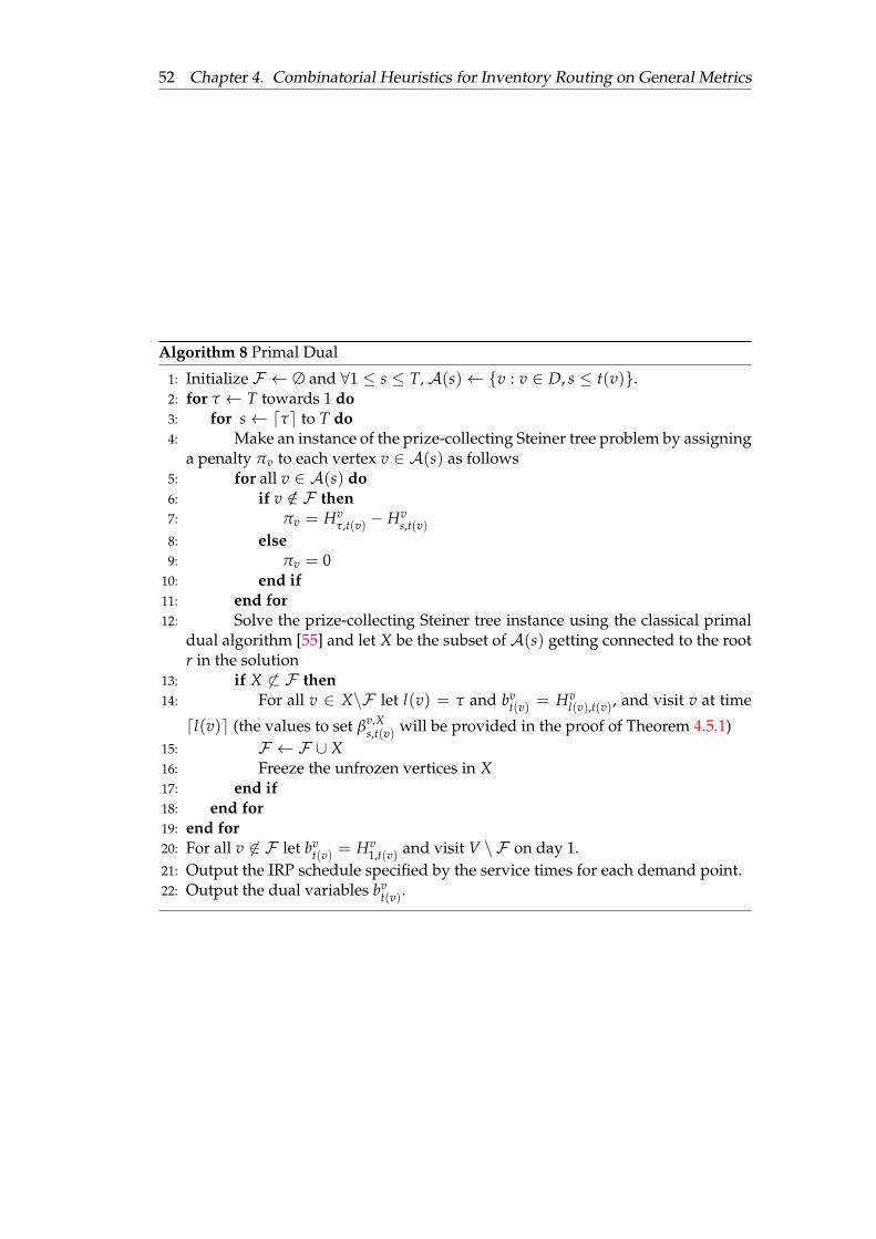
52 Chapter 4. Combinatorial Heuristics for Inventory Routing on General Metrics

Algorithm 8 Primal Dual

1: Initialize F ← ∅ and ∀1 ≤ s ≤ T, A(s)← v : v ∈ D, s ≤ t(v).2: for τ ← T towards 1 do3: for s← dτe to T do4: Make an instance of the prize-collecting Steiner tree problem by assigning

a penalty πv to each vertex v ∈ A(s) as follows5: for all v ∈ A(s) do6: if v /∈ F then7: πv = Hv

τ,t(v) − Hvs,t(v)

8: else9: πv = 0

10: end if11: end for12: Solve the prize-collecting Steiner tree instance using the classical primal

dual algorithm [55] and let X be the subset of A(s) getting connected to the rootr in the solution

13: if X 6⊂ F then14: For all v ∈ X\F let l(v) = τ and bv

t(v) = Hvl(v),t(v), and visit v at time

dl(v)e (the values to set βv,Xs,t(v) will be provided in the proof of Theorem 4.5.1)

15: F ← F ∪ X16: Freeze the unfrozen vertices in X17: end if18: end for19: end for20: For all v 6∈ F let bv

t(v) = Hv1,t(v) and visit V \ F on day 1.

21: Output the IRP schedule specified by the service times for each demand point.22: Output the dual variables bv

t(v).

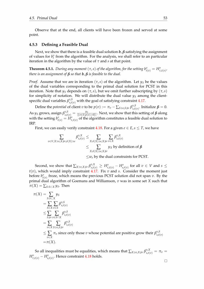
4.5. Primal Dual 53

Observe that at the end, all clients will have been frozen and served at somepoint.

4.5.3 Defining a Feasible Dual

Next, we show that there is a feasible dual solution b, β satisfying the assignmentof values for bv

t from the algorithm. For the analysis, we shall refer to an particulariteration in the algorithm by the value of τ and s at that point.

Theorem 4.5.1. During any moment (τ, s) of the algorithm, for the setting bvt(v) = Hv

τ,t(v),there is an assignment of β so that b, β is feasible to the dual.

Proof. Assume that we are in iteration (τ, s) of the algorithm. Let yS be the valuesof the dual variables corresponding to the primal dual solution for PCST in thisiteration. Note that yS depends on (τ, s), but we omit further subscripting by (τ, s)for simplicity of notation. We will distribute the dual value yS among the client-specific dual variables βv,S

s,t(v) with the goal of satisfying constraint 4.17.

Define the potential of client v to be p(v) := πv −∑S3v,S 63r βv,Ss,t(v). Initialize β = 0.

As yS grows, assign βv,Ss,t(v) =

yS|v∈S:p(v)>0| . Next, we show that this setting of β along

with the setting bvt(v) = Hv

τ,t(v) of the algorithm constitutes a feasible dual solution toIRP.

First, we can easily verify constraint 4.18. For a given e ∈ E, s ≤ T, we have

∑v∈V,X3v,X 63r,δ(X)3e

βv,Xs,t(v) ≤ ∑

X:δ(X)3e,X 63r∑

v∈Xβv,X

s,t(v)

≤ ∑X:δ(X)3e,X 63r

yX by definition of β

≤we by the dual constraints for PCST.

Second, we show that ∑X3v,X 63r βv,Xs,t(v) ≥ Hv

τ,t(v) − Hvs,t(v) for all v ∈ V and s ≤

t(v), which would imply constraint 4.17. Fix v and s. Consider the moment justbefore bv

t(v) froze, which means the previous PCST solution did not span v. By theprimal dual algorithm of Goemans and Williamson, v was in some set X such thatπ(X) = ∑S:S⊂X yS. Then

π(X) = ∑S:S⊂X

yS

= ∑S∈X

∑v∈S

βv,Ss,t(v)

≤∑S 63r

∑v∈S∩X

βv,Ss,t(v)

= ∑v∈X

∑S3v,S 63r

βv,Ss,t(v)

≤ ∑v∈X

πv since only those v whose potential are positive grow their βv,Ss,t(v)

=π(X).

So all inequalities must be equalities, which means that ∑X3v,X 63r βv,Xs,t(v) = πv =

Hvτ,t(v) − Hv

s,t(v). Hence constraint 4.18 holds.

54 Chapter 4. Combinatorial Heuristics for Inventory Routing on General Metrics

4.5.4 Implementation

Here, we provide a simpler implementation of Algorithm 8, which does not re-quire setting dual values and eliminates the loop over s from← dτe to T. In Algo-rithm 8, the purpose of the loop over s is to help determine feasible dual values toset for the variables βv,X

s,t(v) to prove Theorem 4.5.1. However, for purposes of obtain-ing the same primal solution, we do not need to create and solve the PCST instanceper s value. For a fixed τ, no matter which value s takes, the vertices spanned bythe PCST solution all become assigned to the service day τ. Also, for each demandday t(v), there is some round when s takes value t(v), so that the penalty assignedto v is at its highest possible value Hv

τ,t(v). If v gets assigned to be served on day τ

by any s, it would certainly be part of the PCST solution to the instance having thehighest penalty Hv

τ,t(v) − Hvt(v),t(v). So instead of collecting the visits on day τ sepa-

rately through different values of s, we could solve one PCST instance to determinethe visit set for day τ by setting penalty Hv

τ,t(v) for v to collect all visits that couldpossibly have been induced by the largest s. Similarly, the raising of dual valuesbv

t(v) in Algorithm 8 was included to help prove Theorem 4.5.1 and is not neededto determine the primal solution. One last detail we modify is the solution methodfor PCSTs. Algorithm 8 solved PCSTs using [55] so that the dual values of PCSTfrom [55] could be used to determine the dual values to set βv,X

s,t(v), again to provefeasibility. However, for faster solving time, we solve PCSTs using [LLLS18] insteadsince we only need to recover the primal solution at the end regardless of the dualvalues. Further, our implementation is a simplification of the original algorithm thatdiscretizes τ to take only integer values from T to 1. This allows us to use the fastPCST solver of Leitner et al. [LLLS18] in a self-contained manner rather than hav-ing the breakpoints of τ depend on the dual solution for PCST. However, as notedabove, the simplification only finds a primal solution for IRP. The dual values areno longer valid after restricting the breakpoints of τ to only integers. Algorithm 9describes the aforementioned heuristic exactly as implemented.

In addition to the pure Primal Dual heuristic, we test Prioritized local searchinitialized with the solution from the Primal Dual heuristic, which we call PrunedPrimal Dual.

4.6 Benchmark MIP Formulation

In this section, we describe a compact MIP formulation of the IRP, that we usewith modern solvers to establish the benchmark for comparing our solutions. Ourexact MIP formulation for IRP is of size O(N2T) + O(NT2). When the probleminstances get larger, we are however only able to generate lower bounds for thevalue of a solution even using state-of-the-art solvers such as Gurobi Version 7.

As before, xvs,t will be the variable indicating whether to serve (v, t) on day s.

Define a related variable Xvs indicating whether v is visited on day s. Let zuw

s be thevariable indicating whether to use an arc uw on day s. Let huw

s be the continuousvariable representing the amount of total flow through arc uw on day s coming fromthe depot.

Intuitively, the purpose of huws is to enable expressing connectivity in a polyno-

mial number of constraints, in contrast with using a non-compact set of exponen-tially many cut-covering constraints. In Figure 4.6, we provide an example of howthe values of huw

s are set in a feasible solution. Then IRP is modeled by the followingMIP.

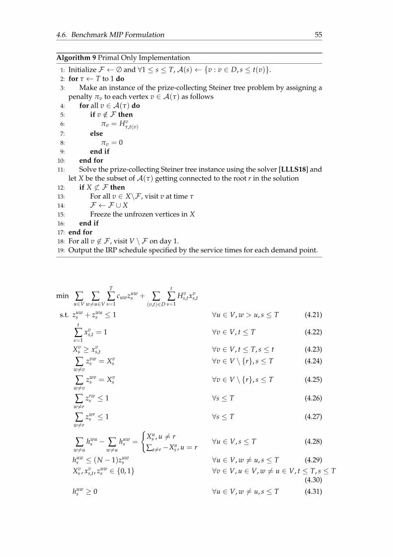
4.6. Benchmark MIP Formulation 55

Algorithm 9 Primal Only Implementation

1: Initialize F ← ∅ and ∀1 ≤ s ≤ T, A(s)← v : v ∈ D, s ≤ t(v).2: for τ ← T to 1 do3: Make an instance of the prize-collecting Steiner tree problem by assigning a

penalty πv to each vertex v ∈ A(τ) as follows4: for all v ∈ A(τ) do5: if v /∈ F then6: πv = Hv

τ,t(v)7: else8: πv = 09: end if

10: end for11: Solve the prize-collecting Steiner tree instance using the solver [LLLS18] and

let X be the subset of A(τ) getting connected to the root r in the solution12: if X 6⊂ F then13: For all v ∈ X\F , visit v at time τ14: F ← F ∪ X15: Freeze the unfrozen vertices in X16: end if17: end for18: For all v 6∈ F , visit V \ F on day 1.19: Output the IRP schedule specified by the service times for each demand point.

min ∑u∈V

∑w 6=u∈V

T

∑s=1

cuwzuws + ∑

(v,t)∈D

t

∑s=1

Hvs,tx

vs,t

s.t. zuws + zwu

s ≤ 1 ∀u ∈ V, w > u, s ≤ T (4.21)t

∑s=1

xvs,t = 1 ∀v ∈ V, t ≤ T (4.22)

Xvs ≥ xv

s,t ∀v ∈ V, t ≤ T, s ≤ t (4.23)

∑w 6=v

zvws = Xv

s ∀v ∈ V \ r, s ≤ T (4.24)

∑w 6=v

zwvs = Xv

s ∀v ∈ V \ r, s ≤ T (4.25)

∑w 6=r

zrws ≤ 1 ∀s ≤ T (4.26)

∑w 6=r

zwrs ≤ 1 ∀s ≤ T (4.27)

∑w 6=u

hwus − ∑

w 6=uhuw

s =

Xu

s , u 6= r

∑a 6=r−Xas , u = r

∀u ∈ V, s ≤ T (4.28)

huws ≤ (N − 1)zuw

s ∀u ∈ V, w 6= u, s ≤ T (4.29)Xv

s , xvs,t, zuw

s ∈ 0, 1 ∀v ∈ V, u ∈ V, w 6= u ∈ V, t ≤ T, s ≤ T(4.30)

huws ≥ 0 ∀u ∈ V, w 6= u, s ≤ T (4.31)

56 Chapter 4. Combinatorial Heuristics for Inventory Routing on General Metrics

67

𝑟

𝑙

𝑗

𝑙 − 1

𝑗 − 1

2

1

𝒍

𝒍 − 𝟏𝟏

𝟎

𝒍 − 𝒋 + 𝟏

FIGURE 4.6: For a fixed day s, suppose that nodes 1, . . . , l are visitedby a cycle in a feasible solution to IRP. To determine the appropriatevalues to set huw

s variables, note that each visited node contributesone unit of flow along the path from from r to itself. Then the flowthrough an arc uw would be the total number of all the paths betweenr and visited nodes that have uw in the path. The labels along thearcs indicate the values that huw

s would take per arc uw. Values of theremaining variables would be set in the obvious ways: zuw

s = 1 if andonly if arc uw is in the cycle, Xv

s = 1 if and only if v ∈ 1, . . . , l,xv

st = 1 if and only if day s is the latest day before or on day t havinga visit to v.

Constraint 4.21 ensures that each edge is used at most once. Constraint 4.22 guar-antees that all demands are satisfied on time. Constraint 4.23 ensures that whenevera demand is served on a specified day, there must be a visit to the client on that day.Constraints 4.24 and 4.25 guarantee that if a vertex is visited, then some in-arc andsome out-arc incident to it must be traversed. Constraints 4.26 and 4.27 limit thenumber of cycles to 1.

We needed a separate case for the fractional degree at r because the depot couldbe served by itself on day s while not building any arcs on day s, which means that∑w 6=r zrw

s and ∑w 6=r zwrs could potentially be 0 even when Xr

s = 1. Constraint 4.28ensures that the net in-flow into any u 6= r corresponds to whether u is visited onthat day, and the net in-flow into r corresponds to the negative of the number ofvertices visited (i.e., out-flow of one per node). Constraint 4.29 requires that on eachday, an arc must be built if there is flow through it from the depot, and the flowallowed is bounded by the maximum possible number of visited nodes.

Solving this MIP directly within MIPGap of 10% was not practical past instancesof size 140 (nodes) by 6 (days) and 50 by 14. We use the lower bound found at 10%MIPGap to compare with the costs from our heuristics.

4.7 Computational Results

Before summarizing the results, we define the necessary parameters involved inthe tests instances. To remain consistent with the problem notation, we still use Nfor the number of clients and T for the number of days. A new parameter H is theamount that the holding cost part of the objective function is multiplied to generateinstances with different trade-offs between routing cost and holding cost. Thus alarger H is oriented towards a solution that pays more attention in optimizing hold-ing versus the routing costs. To measure the quality of our solutions, we examine

4.7. Computational Results 57

the ratio between the cost of a heuristic solution and the lower bound on the optimalcost found by Gurobi solving the MIP. We call this ratio the gap between the respec-tive costs. We implemented all the heuristics we described earlier, to compare themagainst the lower bounds from the benchmark MIP model described above.

1. Local search with DELETE (Algorithm 1).

2. Local search with ADD (Algorithm 2).

3. Prioritized Local Search (Section 4.3.3).

4. Greedy (Section 4.4.3).

5. Pruned Greedy - this is the prioritized local search algorithm applied to aninitial solution obtained by Greedy.

6. Primal Dual (Section 4.5.4).

7. Pruned Primal Dual - this is the prioritized local search algorithm applied toan initial solution obtained by Primal Dual.

Here is a summary of the performance of the various methods we implemented(details of the data generation model are in the next section).

1. The heuristics achieving the best gap and solving time are the prioritized localsearch and the local search with ADD steps, shown in Figure 4.7.

2. Greedy has the largest gaps among all heuristics according to Figures 4.7, 4.8,and 4.9 because picking low density sets to cover demands does not directlyhelp lower the final cost of the IRP solution. Greedy also incurs the longestsolving time due the computationally expensive nature of picking low densitysets.

3. The prioritized local search starting with greedy or primal dual solutions hadworse gaps than simply starting with the solution after local search with ADDsaccording to Figures 4.7, 4.8, and 4.9. The worse performance could be causedby greedy and primal dual being closer to locally optimal but still somewhatfar from the lower bound.

4. From Figure 4.7, as H increases, greedy’s gap decreases dramatically becauselow H values incentivize greedy to pick large sets to start with, which leavesno room to cover demands optimally. The larger H becomes, the more oppor-tunities arise for the sets to be more fine tuned. Primal dual and the three localsearch heuristics have gaps that initially increase up to some H value within[2, 3], then decrease thereafter. This pattern occurs because mid-range H val-ues create instances with more balanced trade-offs between routing cost andholding cost, which correspond to higher difficulty to solve.

5. As T increases, primal dual’s gap worsens according to Figure 4.9 becauseprimal dual tends to build denser visits than needed because the backwardssweep construction of visit sets cannot account for potentially early visits serv-ing late deadlines.

The rest of this section explains these points in more detail.The heuristics were implemented in C++ on an Intel Xeon processor X5680, 3.33

GHz machine with 8 GB RAM. A copy of the code and data used to conduct the

58 Chapter 4. Combinatorial Heuristics for Inventory Routing on General Metrics

experiments will soon be available on github. Since solving the MIP was the majorbottleneck in completing the experiments, we allowed multiple threads for the MIPto speed up the solving time. The MIP was solved by Gurobi Version 7 on defaultsettings using 8 threads. Each heuristic uses 1 thread. We report the run times di-rectly without accounting for number of threads. Next, we describe how the testinstances were generated. Recall that we defined the actual versions of the heuris-tics implemented in their corresponding sections. We then show their performancein cost and runtime relative to each of the three varying parameters.

4.7.1 Data Generation Model

We follow the same generation model of the largest instances tested in Archettiet al. [8], except that our model has no capacity constraints at vehicles and storelocations. To find how the heuristics perform on different types of instances, wechoose three parameters N, T, and H to vary (one at at time). For each setting ofparameter values, we generate 100 test instances.

• Time horizon T = 6, 8, . . . , 18

• Number of clients N = 110, 120, . . . , 160

• Demands dvt randomly generated as an integer in the interval [10, 100]

• Unit holding cost hv randomly generated real number in the interval [0.01, 0.05]

• Transportation cost cuv =√(Xu − Xv)2 + (Yu −Yv)2, with each coordinate of

(Xu, Yu) randomly generated as an integer in [0, 500]

We have an additional parameter H = .01, 0.51, . . . , 6.01 which we use as the scal-ing factor for the holding cost to generate a wide variety of instances. Our objectivefunction relative to H is r(S) + H × h(S), where r(S) is the routing cost and h(S) isthe holding cost of a solution S.

4.7.2 Performance Evaluation

For each heuristic, we plot two values as H, N, or T varies: the gap and runningtime. Recall that the gap is the ratio between the heuristic’s solution cost and thelower bound found for the optimal cost of the MIP model. Henceforth, all gap orrunning time values mentioned refer to the average values over the 100 instancesper choice of parameter values.Varying H

Here, N and T are fixed to 100 and 6, respectively. The holding cost scale H variesfrom 0.01 to 6.01 at increments of 0.5. Results that require lower bound from the MIPgo up to only H = 4.51 due to high running times of the MIP and the large numberof instances per parameter value. We compare the performance of the three localsearch heuristics, pure greedy, greedy with pruning, pure primal dual, and primaldual with pruning.

First, we state the results for the gap.

• Greedy has decreasing gaps as H increases, starting at 2.33 when H = 0.01 to1.53 when H = 4.51.

4.7. Computational Results 59

• Pruned greedy drastically improves upon greedy due to the additional prun-ing by prioritized local search and has the largest gap of 1.11 at H = 3.01. Asmentioned before, the mid-range values of H correspond to harder instancesbecause the trade-off between the routing cost and holding cost is in the mid-dle.

• Primal dual has its largest gap of 1.19 at H = 2.51.

• Pruned primal dual’s gaps increase as H increases, starting from 1.01 at H =0.01 to 1.11 at H = 4.51. It might be the case that the gap would eventually ta-per off at a larger value of H, but we do not have the lower bounds to comparewith due to the large solving times of the MIP.

• For DELETE local search, the gap is largest at 1.1 for H at 2.51 and 3.01.

• For ADD and prioritized local searches, the gap is at most 1.05 for all valuesof H. The values of H for which they have their highest gaps occur at 2.01 and2.51. Since ADD and DELETE-ADD are richer operations in their use of thePCST solutions, we expect them to reach close to optimality. The prioritizedlocal search and local search with ADDs have similar gaps because the solutionfrom ADD is already nearly optimal and there is little room to improve the cost.

In summary, the heuristics in order of lowest to highest gaps are local search withADDs, prioritized local search, local search with DELETEs, pruned greedy, prunedprimal dual, primal dual, and greedy.

Next, we examine the running time of each heuristic.

• The MIP requires over 47 seconds to solve for H = 0.01 and over 768 secondsat H = 4.51.

• Greedy and pruned greedy take the longest to solve among the heuristics.Their solving times start at more than 19 seconds when H = 0.01 and increaseto over 24 seconds at H = 6.01.

• Pruned primal dual requires no more than 3 seconds for all values of H.

• Each of the three local searches (prioritized, ADD, DELETE) take less than 1second on average for instances with any value of H.

• Primal dual also takes under 1 second throughout all instances.

To summarize, the heuristics in order running times from the fastest to slowest arelocal search with DELETE-ADDs, primal dual, local search with ADDs, Prioritizedlocal search, pruned primal dual, greedy and pruned greedy.

Local search with ADDs prevails as the strongest of the heuristics with a gap ofat most 1.05 throughout and runtime of less than 1 second at H = 4.51, which isnearly three orders of magnitude faster than the MIP at H = 4.51.Varying N

Here, T and H are fixed to 6 and 2.6, respectively. The number of clients N variesfrom 110 to 160 at increments of 10. Due to limited computation time, results whichrequire MIP values are restricted to N ≤ 140.

First, we provide the gaps for each heuristic. The gap values of the heuristics didnot form any particular patterns with respect to N.

• Among all methods, greedy has the highest gap of 1.57 to 1.58.

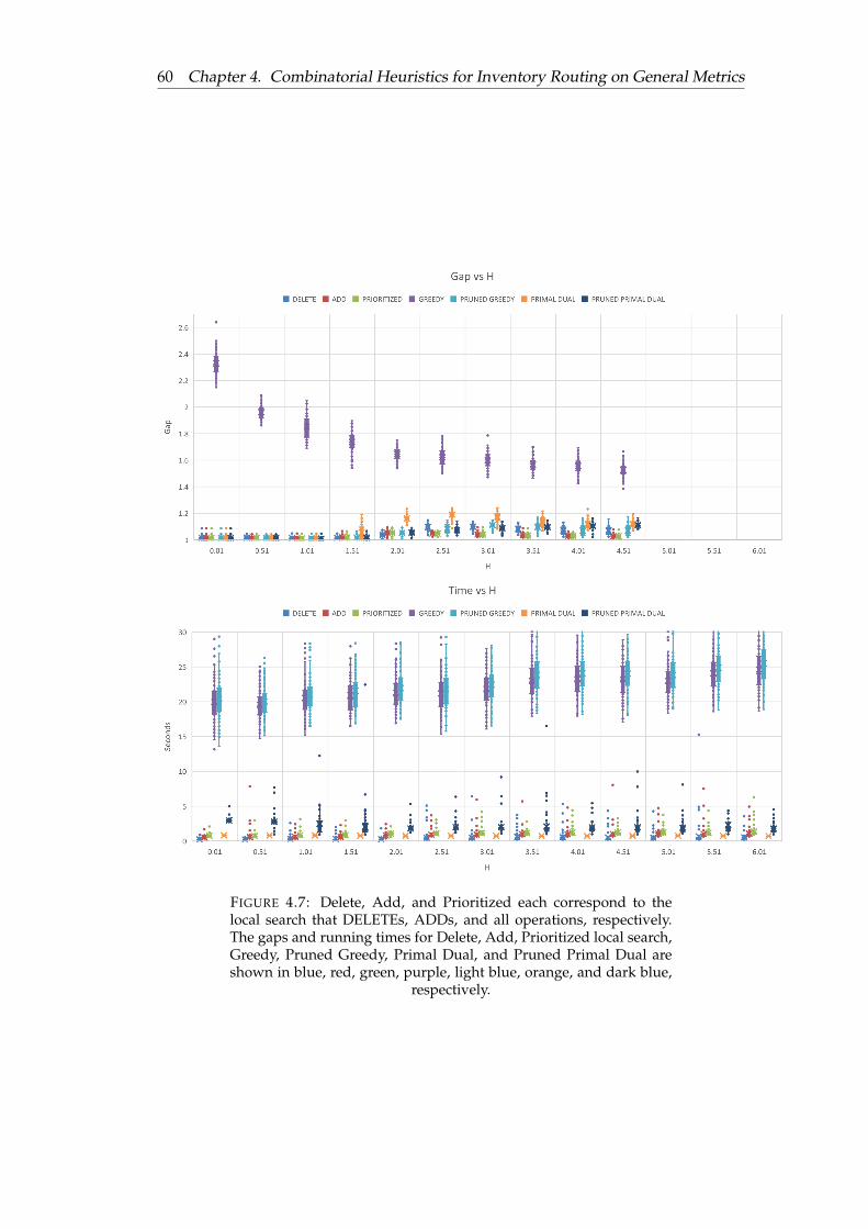
60 Chapter 4. Combinatorial Heuristics for Inventory Routing on General Metrics

FIGURE 4.7: Delete, Add, and Prioritized each correspond to thelocal search that DELETEs, ADDs, and all operations, respectively.The gaps and running times for Delete, Add, Prioritized local search,Greedy, Pruned Greedy, Primal Dual, and Pruned Primal Dual areshown in blue, red, green, purple, light blue, orange, and dark blue,

respectively.

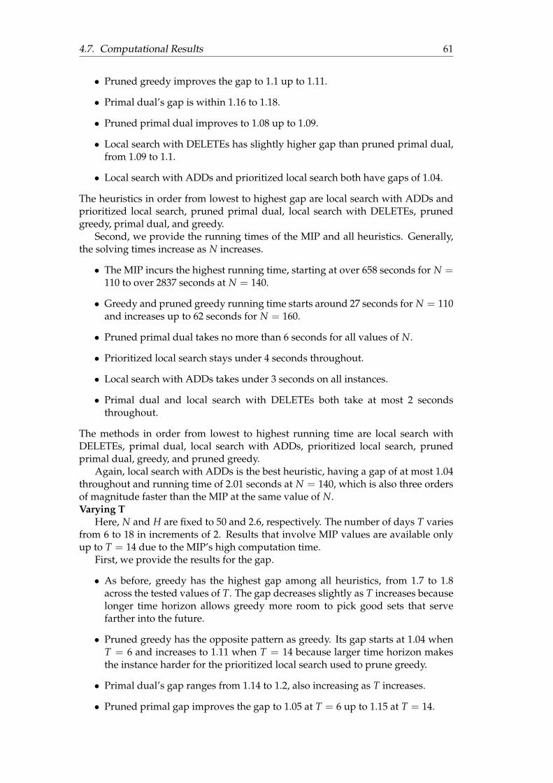
4.7. Computational Results 61

• Pruned greedy improves the gap to 1.1 up to 1.11.

• Primal dual’s gap is within 1.16 to 1.18.

• Pruned primal dual improves to 1.08 up to 1.09.

• Local search with DELETEs has slightly higher gap than pruned primal dual,from 1.09 to 1.1.

• Local search with ADDs and prioritized local search both have gaps of 1.04.

The heuristics in order from lowest to highest gap are local search with ADDs andprioritized local search, pruned primal dual, local search with DELETEs, prunedgreedy, primal dual, and greedy.

Second, we provide the running times of the MIP and all heuristics. Generally,the solving times increase as N increases.

• The MIP incurs the highest running time, starting at over 658 seconds for N =110 to over 2837 seconds at N = 140.

• Greedy and pruned greedy running time starts around 27 seconds for N = 110and increases up to 62 seconds for N = 160.

• Pruned primal dual takes no more than 6 seconds for all values of N.

• Prioritized local search stays under 4 seconds throughout.

• Local search with ADDs takes under 3 seconds on all instances.

• Primal dual and local search with DELETEs both take at most 2 secondsthroughout.

The methods in order from lowest to highest running time are local search withDELETEs, primal dual, local search with ADDs, prioritized local search, prunedprimal dual, greedy, and pruned greedy.

Again, local search with ADDs is the best heuristic, having a gap of at most 1.04throughout and running time of 2.01 seconds at N = 140, which is also three ordersof magnitude faster than the MIP at the same value of N.Varying T

Here, N and H are fixed to 50 and 2.6, respectively. The number of days T variesfrom 6 to 18 in increments of 2. Results that involve MIP values are available onlyup to T = 14 due to the MIP’s high computation time.

First, we provide the results for the gap.

• As before, greedy has the highest gap among all heuristics, from 1.7 to 1.8across the tested values of T. The gap decreases slightly as T increases becauselonger time horizon allows greedy more room to pick good sets that servefarther into the future.

• Pruned greedy has the opposite pattern as greedy. Its gap starts at 1.04 whenT = 6 and increases to 1.11 when T = 14 because larger time horizon makesthe instance harder for the prioritized local search used to prune greedy.

• Primal dual’s gap ranges from 1.14 to 1.2, also increasing as T increases.

• Pruned primal gap improves the gap to 1.05 at T = 6 up to 1.15 at T = 14.

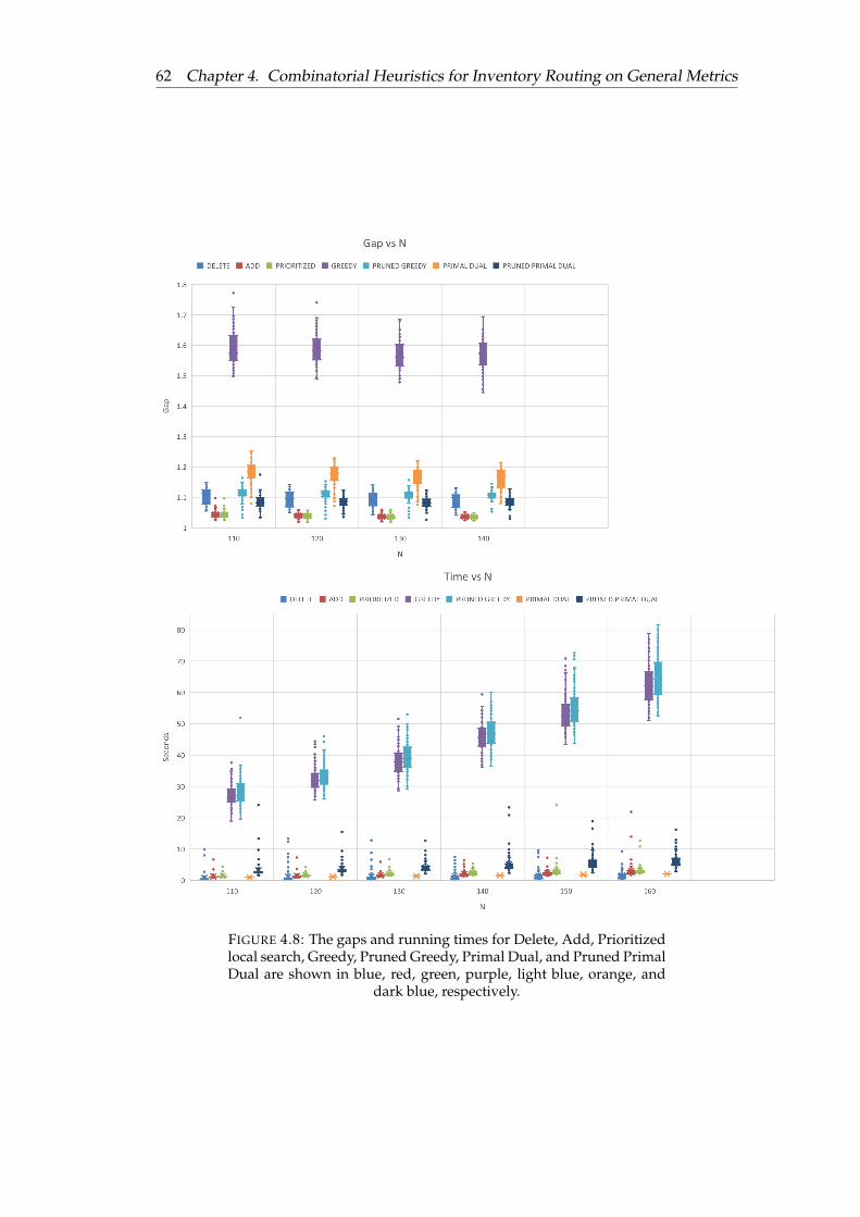
62 Chapter 4. Combinatorial Heuristics for Inventory Routing on General Metrics

FIGURE 4.8: The gaps and running times for Delete, Add, Prioritizedlocal search, Greedy, Pruned Greedy, Primal Dual, and Pruned PrimalDual are shown in blue, red, green, purple, light blue, orange, and

dark blue, respectively.

4.7. Computational Results 63

• Local search with DELETEs’ gap does not exhibit any trend with respect to T.The gap ranges from 1.03 to 1.09.

• Local search with ADDs and prioritized local search both have gaps startingfrom 1.03 at T = 6 to 1.08 at T = 14.

In order from lowest to highest gap, the heuristics are local search with ADDs andprioritized local search, local search with DELETEs, pruned primal dual, prunedgreedy, primal dual, and greedy.

Second, we show the solving times. As expected, the solving times all increaseas T increases.

• MIP solves in over 10 seconds for T = 6 and increases to over 1481 seconds atT = 14.

• Greedy and pruned greedy take around 6 seconds at T = 6, increasing to 30seconds at T = 18.

• Pruned primal dual requires less than 3 seconds on all instances.

• Primal dual, prioritized local search, and local search with ADDs take under 2seconds throughout.

• Local search with DELETEs take under 1 second throughout.

The methods in increasing order of solving time are local search with DELETEs, localsearch with ADDs, prioritized local search, primal dual, pruned primal dual, greedy,and pruned greedy.

As expected, local search with ADDs has the best gap of at most 1.08 throughall test instances and a solving time of less than 1 second for T = 14, which is threeorders of magnitude faster than the MIP at T = 14.

4.7.3 Conclusions

In this chapter, we introduced new local search, greedy, and primal dual heuris-tics that exploit the PCST as intermediate steps towards obtaining near-optimal so-lutions for IRP. We used the PCST subroutine to design very large neighborhoodsearch methods, as well as to find low density sets to serve for the solution in Greedyand good primal visits for the solution for a primal-dual method. We proved a per-formance guarantee for Greedy and showed how the PCST method provides theneeded properties of the solutions in these heuristics. Thus a main contribution ofour work has been to extend the theoretical insights from the work of [49] in usingthe PCST problem as an effective tool to solve IRP. Among the different heuristics weexperimented with, the local search with ADDs performed the best. For 140 by 6 in-stances, it was able to reach within 1.04 factor of optimal cost with a speedup of threeorders of magnitude compared to solving the MIP using Gurobi. Similarly, for 50 by14 instances, it reaches 1.08 factor of optimal cost with similar speedups. Gener-ally, primal dual and greedy were less effective than the local search based methodsbecause their better starting solution structure affords less flexibility in the later pri-oritized local search pruning phase. In all instance sets, greedy had the highest gapand the longest running time. An interesting research direction for future work is toextend the PCST-based approaches to the more general case of IRP with vehicle andinventory capacities.

64 Chapter 4. Combinatorial Heuristics for Inventory Routing on General Metrics

FIGURE 4.9: The gaps and running times for Delete, Add, Prioritizedlocal search, Greedy, Pruned Greedy, Primal Dual, and Pruned PrimalDual are shown in blue, red, green, purple, light blue, orange, and

dark blue, respectively.

4.8. Acknowledgments 65

4.8 Acknowledgments

We would like thank Afshin Nikzad for his contribution to the idea of solvingPCSTs within the primal dual heuristic.

67

Chapter 5

Deadline Inventory RoutingProblem

5.1 Introduction

The Deadline Inventory Routing Problem (Deadline IRP) is a new variant of theclassical IRP [25]. In the classical single-depot IRP [23, 29, 25, 26], a set of client de-mand locations in a metric containing the depot is given, and for a planning horizonof T days, a daily demand at each client location is specified. The goal is to comeup with vehicle routing schedules in each of the T days to stock the client demandsbefore they materialize. However, early stocking at a location incurs a location- andduration-specific inventory holding cost that are also specified. If we assume thedaily replenishing vehicle has infinite capacity, the distance traveled by the vehiclein a daily route translates to a routing cost. The goal of IRP is to find daily vehi-cle schedules for the T days that deliver enough supply at each location to meet alldaily demands and minimizes the sum of inventory holding costs for units suppliedahead of their demand and the daily routing costs of the vehicle, over the T days.

The Deadline IRP (DIRP) replaces the daily client demands with a deadline forrevisit. In other words, if the vehicle visits a location v at time t, this results ina requirement that the next visit of the vehicle to this location must occur by thetime the resources delivered at v are depleted - this sets up a deadline for the nextvisit which is t + Dv where Dv denotes the depletion time. The routing costs areunchanged from the classical IRP formulation. One example of where this alternateformulation appears is in the replenishment of automatic teller machines (ATMs)with cash [4]: based on the currency demand at each location and the servicerequirements of the bank, each visit automatically triggers a deadline for the nextvisit.

Problem Definition. Formally, the Deadline Inventory Routing Problem is given asinput the following.

• a set V of vertices/clients on a metric c that defines the routing costs,

• a root node r ∈ V from which an uncapacitated supply vehicle starts,

• a discrete time horizon 1, 2, . . . , T over which the clients require service, and

• a length Dv of time called the depletion time for each client v that indicates howlong the clients will last from the previous visit before its supplies run out.

The objective of deadline IRP is to minimize the vehicle routing cost while supplyingthe clients within their deadlines over the time horizon. We assume that the dailyvehicle route is a tour that starts and ends in the root. We relax this to be a Steiner

68 Chapter 5. Deadline Inventory Routing Problem

tree connecting the root to the clients visited that day with a loss of a factor of 2 inthe approximation guarantee in the sequel1. Note again that the deadlines are visitdependent.

5.2 Related Work

As mentioned before, our problem can be seen as a special case of the INVEN-TORY ROUTING PROBLEM (IRP) [34]. Here, clients (vertices) have their own storagewith a certain capacity and for each day a demand is specified. The clients pay hold-ing cost over their inventory. However, omitting inventory cost, we can interpret ourproblem as such an inventory routing problem in which the demand at any givenlocation is the same every day.

Another closely related problem is the PERIODIC LATENCY PROBLEM [35], whichfeatures the recurring visits requirement of DIRP. We are given recurrence length qifor each client i and travel distances between clients. Client i is considered served ifit is visited every qi time units. The server does not return to the depot at the end ofeach time unit (e.g. day), but keeps moving continuously between clients at uniformspeed. Another difference between PERIODIC LATENCY PROBLEM and DIRP is theobjective function. Coene et al. [35] study two versions of the problem: one thatmaximizes the number of served clients by one server, and one that minimizes thenumber of servers needed to serve all clients. They resolve the complexity of theseproblems on lines, circles, stars, trees, and general metrics.

A more restrictive problem than DIRP, but with a compact input size is knownunder the guise of PINWHEEL SCHEDULING. It has been introduced to model thescheduling of a ground station to receive information from a set of satellites withoutdata loss. In terms of our problem no more than one vertex can be replenished perday and all distances to the depot are the same; the interesting question here is ifthere exists a feasible schedule for replenishing the vertices. Formally, a set of jobs1, ..., n with periods p1, ..., pn is given, and the question is whether there exists aschedule σ : N → 1, .., n such that j ∈ ⋃t+pj

k=t+1 σk, ∀t ≥ 0 and ∀j. Note thatthe compact representation of time in Pinwheel Scheduling makes its complexityincomparable to that of our problem.

PINWHEEL SCHEDULING was introduced by Holte et al. [59], who showed thatit is contained in PSPACE. The problem is in NP if the schedule σ is restricted to onein which for each job the time between two consecutive executions remains constantthroughout the schedule. In particular this holds for instances with density ρ =

∑j 1/pj = 1 [59]. They also observed that the problem is easily solvable when ρ ≤ 1and the periods are harmonic, i.e. pi is a divisor of pj or vice versa for all i and j. Asa corollary, every instance with ρ ≤ 1

2 is feasible.Chan and Chin [31] improved the latter result by giving an algorithm that pro-

duces a feasible schedule for PINWHEEL SCHEDULING whenever ρ ≤ 23 . In [30],

they improved this factor to 710 . Later, Fishburn and Lagarias [47] showed that every

instance with ρ ≤ 34 has a feasible schedule. All these papers work towards the con-

jecture that there is a feasible schedule if ρ ≤ 56 . That this bound is tight can be seen

by the instance with p1 = 2, p2 = 3 and p3 = M, with M large. This instance cannotbe scheduled, but has a density of 5

6 +1M .

1This relaxation of the tour to be a tree is purely for the sake of simplification of the approximationalgorithms for finding such a route - the algorithms are better understood for trees rather than tours.Moreover, we can convert trees to tours in the end with a further loss of factor of 2 in metrics using anEuler walk on the tree.

5.3. Approximation Algorithms 69

The complexity of PINWHEEL SCHEDULING has been open since it was intro-duced. It was only recently shown by Jacobs and Longo [60] that there is no pseu-dopolynomial time algorithm solving the problem unless SAT has an exact algo-rithm running in expected time nO(log n log log n), implying for example that the ran-domized exponential time hypothesis fails to hold [24, 36]. Since the latter is un-likely, one could conclude that PINWHEEL SCHEDULING is not solvable in pseu-dopolynomial time. It remains open whether the problem is PSPACE-complete.

Similar to PINWHEEL SCHEDULING, the k-SERVER PERIODIC MAINTENANCE

PROBLEM [72, 15, 42] has n jobs, each with a specified periodicity and a process-ing time. Each server may serve at most one job per time unit. However, job i isrequired to be served exactly every mi days apart rather than within every mi days.The case k = 1, cj = 1 for all j is analogous to PINWHEEL SCHEDULING, except forthe exact periodicity constraint. For any k ≥ 1, Mok et al. [72] have shown it isNP-complete in the strong sense. For the special case when mi are multiples of eachother or when there are at most 2 different periodicities, they have shown it is in P.

Other related problems with a compact input representation include real-timescheduling of sporadic tasks [14, 20], where we are given a set of recurrent tasks. Ona single machine, EDF (Earliest Deadline First) is optimal. However, we remark thatthe complexity of deciding whether a given set of tasks is feasible has been open fora long time and only recently proved showing that it is coNP-hard to decide whethera task system is feasible on a single processor even if the utilization is bounded [43].

Another related problem is the BAMBOO GARDEN TRIMMING PROBLEM intro-duced by Gasieniec et al. [51]. There are n bamboos, each having a given growthrate, which may be viewed as inducing a periodicity. On each day, a robot may trimat most one bamboo back to height 0. The goal is to minimize the maximum heightof the bamboos. Gasieniec et al. provide a 4-approximation for the general case anda 2-approximation for balanced growth rates.

The full paper including results for DIRP on special metrics appeared in the pro-ceedings of the 13th Latin American Symposium [21].

5.3 Approximation Algorithms

In this section, we study the design of near-optimal periodic solutions for DIRP.First we show that the periods can be restricted to be of the same order of magnitudeas the maximum client deadline, and all deadlines can be assumed to be powers oftwo with a constant factor loss in optimality. Next, we prove a logarithmic approx-imation algorithm by using the ideas of increasing and synchronized solutions thatwe define and approximate.

We reduce arbitrary Deadline Inventory Routing Problems to those whose de-pletion times are powers of 2 losing only a constant factor.

Lemma 5.3.1. Let Π be a Deadline Inventory Routing Problem instance. For a client v,denote its depletion time by Tv. For any time t, let r(t) be the largest power of 2 not exceedingt. Let Π′ be the Deadline Inventory Routing Problem instance having the same vertex set asΠ, but depletion time r(Tv) for each v ∈ V. Let OPT and OPT′ be the minimum cost of Πand Π′. Then any solution feasible for Π′ is feasible for Π, and OPT′ ≤ 4OPT.

Proof. Feasibility for Π′ implies feasibility for Π by r(Tv) ≤ Tv for all v. To show thatOPT′ ≤ 4OPT, we show that any solution S of Π can be converted to a solution S′

of Π′ such that c(S′) ≤ 4c(S). Given a solution S to Π, let S be the solution such thatfor each t, copy the tree of S at time t to time d t

2e in addition to the original tree attime t.

70 Chapter 5. Deadline Inventory Routing Problem

We claim that S is feasible to the first half subinstance of Π′. To show this, observeno S visit between tk and tk+1 implies no S visit between 2tk and 2tk+1. If tk+1 − tk ≥r(Tv), then 2tk+1 − 2tk ≥ 2d Tv

2 e ≥ Tv, which would imply that S was not feasible toΠ. So S must be feasible to at least the first half subinstance of Π′. By construction,c(S) ≤ 2c(S).

Let S′ be the solution that copies the trees of S in the first half of the instance tothe second half and retains the same first half as S. Then S′ is feasible to the entireinstance Π′, and c(S′) ≤ 2c(S) ≤ 4c(S).

Consider a powers of 2 instance of the Deadline Inventory Routing Problem inwhich depletion times span from 20 to 2L. Denote by V2j the set of vertices whohave depletion time 2j; so V = V1 ∪ · · · ∪ V2L . Define a synchronized solution tobe one which, for each l ≤ L, visits exactly V1 ∪ · · · ∪ V2l on day 2l . Given a treeT covering some subset of V, we say that T is non-decreasing with respect to theDeadline Inventory Routing Problem instance if for each v ∈ V(T), v ∈ V2j impliesthat the r-v path in T contains only vertices from V2l for l ≤ j.

Proposition 5.3.2. Given a solution S to a powers of 2 instance of Deadline InventoryRouting Problem, if the tree in S for each day is non-decreasing, then there is a synchronizedsolution S′ of cost at most c(S).

Proof. We shall use each edge of S at most once to build the trees for S′. First, weknow that for each j ≤ L, every vertex of V2j occurs at least once per time windowof length 2j − 1 in S. So S has paths that reach all of V2j for each window of the form[k2j + 1, (k + 1)2j]. We will use this to build paths for each j that reach V2j on all daysthat are multiples of 2j.

In the base case, we build paths between r and v for all v ∈ V20 once for eachday by using exactly the same V20-reaching paths in S. For the remaining vertices,we build the synchronized solution inductively. Starting from j = 1 to L, for eachk within 0 to 2L−j − 1, take the union of all paths of S occurring between V2j−1 andV2j within days [k2j + 1, (k + 1)2j] and place the edge union at time (k + 1)2j. Notethat we already have paths from r to V2j−1 per day of the form l2j−1 from the earlierrounds. So the current round has guaranteed to reach V2j per day of the form l2j. Atthe end, we have a solution that visits each V2j on all days that are multiples of 2j

and uses each edge of S only once.

Now, we show that arbitrary trees can be approximated by nondecreasing treeswithin logarithmic factor. To do so, we use a tree pairing lemma of Klein andRavi’s [64] that will help us construct the appropriate nondecreasing trees. We in-clude the proof for completeness.

Lemma 5.3.3. [64] Given any tree T and an even subset S of its vertices, there is a pairingof vertices covering S such that the tree-path induced by the pairs are edge-disjoint.

Proof. Let T be a tree on vertex set V and S ⊂ V. For a pairing P, let φ(P) be thetotal length of the paths induced by the pairs in P. We will show that a pairing P∗

minimizing φ(P∗) has all edge-disjoint pair-induced paths. Suppose there are pairsu1, v1 and u2, v2 that share some edge a, b. WLOG, assume that u1 and u2are closer to a than b and v1 and v2 are closer to b than a. Then repairing the fourvertices to u1, u2 and v1, v2 reduces the total length of the paths. So a pairingminimizing the total length cannot have any pairs that overlap.

Using the tree pairing lemma 5.3.3, we will construct nondecreasing trees to ap-proximate arbitrary trees. First we define the notations needed for the algorithm.

5.3. Approximation Algorithms 71

For v ∈ V, let l(v) be the label of the class v belongs to, i.e. Vl(v) 3 v. A nonde-creasing arc a(u, v) of u, v is the arc between u and v that points from the vertexof lower label to the vertex of higher label (ties are broken arbitrarily). The vertexof lower (higher) label between u and v is denoted by L(u, v) (H(u, v)). Wedenote by U the unpaired vertices and A the arcs of the nondecreasing tree beingconstructed.

1: Initialize U ← V and A← ∅.2: while |U| > 0 do:3: Find an edge-disjoint pairing P of a largest even subset of U.4: for u, v ∈ P do:5: A← A ∪ a(u, v).6: U ← U \ H(u, v).7: end for8: end while

Proposition 5.3.4. Given an arbitrary tree T of cost c(T) with respect to vertex setsV0, . . . , VL, there is a nondecreasing tree of cost at most dlog2 nec(T).

Proof. Consider an instance of DIRP. Let T be a tree. We will construct a nonde-creasing tree T′ by iteratively pairing off the vertices and directing each pair in anondecreasing manner.

In the algorithm, we apply the pairing procedure dlog2 ne times to get a nonde-creasing tree of the desired cost. In each round, we pair a largest subset of V suchthat the pairs induce edge disjoint paths in T. Then we direct each pair u, v fromthe vertex of lower label to the vertex of higher label according to the labeling l anddelete the vertex of higher label from consideration. These arcs are added to thearc set of T′. We can think of each pair as a connected component represented bythe vertex of the lower label. In the end, T′ is finalized when no unpaired verticesremain. Note that picking the vertex of minimum label as the representative perconnected component ensures that the final tree is indeed an out-arborescence fromthe vertex of smallest label.

In each round, we used each edge of T at most once since all pair-induced pathswere edge-disjoint. Let κ(t) be the number of vertices at the beginning of round t.Since each round paired off either all vertices or all but vertex, we have κ(t) = dκ(t−1)/2e. So the total number of rounds is dlog2 ne. Hence c(T′) ≤ dlog2 nec(T).

Theorem 5.3.5. There is a O(log n)-approximation for the Deadline Inventory RoutingProblem.

Proof. Given an DIRP instance, OPT denote the cost of an optimal solution. Let ρSTbe the best known approximation ratio for Steiner tree. We will construct a synchro-nized solution to DIRP that has cost at most O(log n)OPT. Note that the subset ofclients to visit per day is completely determined in any synchronized solution. Sooptimal synchronized solutions may be approximated within ρST factor. As ρST isconstant, it suffices to show that optimal synchronized solutions to DIRP are withinO(log n) factor from OPT.

By proposition 5.3.4, there is a nondecreasing solution S′ to DIRP of cost at mostdlog2 neOPT. By Proposition 5.3.2 on each tree of S′, there is a synchronized solutionS to DIRP of cost c(S′). So an optimal synchronized solution to DIRP has cost at mostc(S) ≤ c(S′) ≤ dlog2 neOPT.

However, the above method cannot be improved. There is a class of instancesfor which the cost of optimal solutions is logarithmic factor away from the cost of

72 Chapter 5. Deadline Inventory Routing Problem

optimal monotone solutions. The class of examples is due to a co-author, ThomasBosman.

Proposition 5.3.6. There exists a class of instances in which there is a logarithmic optimal-ity gap between the optimal and the optimal non-decreasing solution.

Consider the following sequence of sequences (a0, a1, . . .) where a0 = (1) andai+1 is generated by alternatingly taking an element from ai and then from the se-quence bi = (2i + 1, 2i + 2, . . . , 2i+1). For example:

• a0 = 1

• a1 = 1, 2

• a2 = 1, 3, 2, 4

• a3 = 1, 5, 3, 6, 2, 7, 4, 8

• · · ·Then define the (unweighted) graph Gi as the path graph with 2i vertices, where

the jth vertex has depletion time 2aij−1. See Figure 5.1 for an example.

FIGURE 5.1: Illustration of G2, (depletion times in circles)

1 4 2 8

The minimum spanning tree in Gi costs 2i− 1. It is easy to check that the decreas-ing spanning tree produced by Lemma 5.3.3 costs i2i−1. Moreover, since the solutionproduced attaches every vertex to a nearest vertex with lower depletion time, it mustbe optimal.

To show tightness of our main theorem, we will define another class of graphsHi for i ≥ 1 that are constructed from Gi. The idea is to make τj copies of eachterminal j, and then connect them in a regular way, for example like in Figure 5.2.

FIGURE 5.2: Illustration of H2

τi = 1 τi = 4 τi = 2 τi = 8

Formally Hi is constructed as follows. For simplicity of description, we assumethat Gi is planarly embedded from left to right, and we assume that we keep a planarembedding of Hi during construction.

We first copy node 1 to Hi. Now we work from left to right, starting from thesecond node. When we are at node j, we put τj copies of j vertically above eachother and to the right of the copies of j− 1 in Hi. Then we connect them to the copiesof j− 1 in Hi such that the graph remains planar and all copies of j− 1 have the samedegree, and all copies of j have the same degree. This can be done in only one way.Furthermore we identify vertex 1 with the depot.

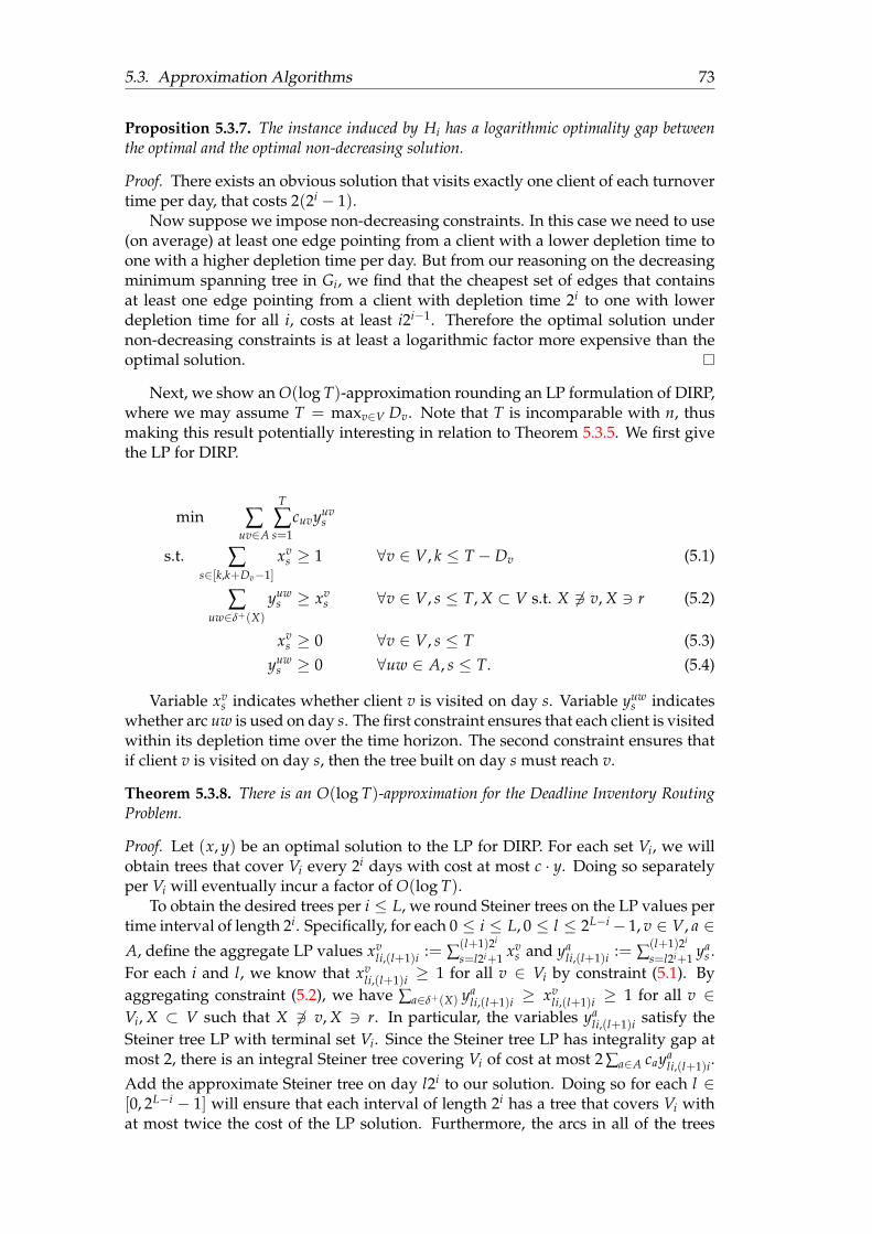
5.3. Approximation Algorithms 73

Proposition 5.3.7. The instance induced by Hi has a logarithmic optimality gap betweenthe optimal and the optimal non-decreasing solution.

Proof. There exists an obvious solution that visits exactly one client of each turnovertime per day, that costs 2(2i − 1).

Now suppose we impose non-decreasing constraints. In this case we need to use(on average) at least one edge pointing from a client with a lower depletion time toone with a higher depletion time per day. But from our reasoning on the decreasingminimum spanning tree in Gi, we find that the cheapest set of edges that containsat least one edge pointing from a client with depletion time 2i to one with lowerdepletion time for all i, costs at least i2i−1. Therefore the optimal solution undernon-decreasing constraints is at least a logarithmic factor more expensive than theoptimal solution.

Next, we show an O(log T)-approximation rounding an LP formulation of DIRP,where we may assume T = maxv∈V Dv. Note that T is incomparable with n, thusmaking this result potentially interesting in relation to Theorem 5.3.5. We first givethe LP for DIRP.

min ∑uv∈A

T

∑s=1

cuvyuvs

s.t. ∑s∈[k,k+Dv−1]

xvs ≥ 1 ∀v ∈ V, k ≤ T − Dv (5.1)

∑uw∈δ+(X)

yuws ≥ xv

s ∀v ∈ V, s ≤ T, X ⊂ V s.t. X 63 v, X 3 r (5.2)

xvs ≥ 0 ∀v ∈ V, s ≤ T (5.3)

yuws ≥ 0 ∀uw ∈ A, s ≤ T. (5.4)

Variable xvs indicates whether client v is visited on day s. Variable yuw

s indicateswhether arc uw is used on day s. The first constraint ensures that each client is visitedwithin its depletion time over the time horizon. The second constraint ensures thatif client v is visited on day s, then the tree built on day s must reach v.

Theorem 5.3.8. There is an O(log T)-approximation for the Deadline Inventory RoutingProblem.

Proof. Let (x, y) be an optimal solution to the LP for DIRP. For each set Vi, we willobtain trees that cover Vi every 2i days with cost at most c · y. Doing so separatelyper Vi will eventually incur a factor of O(log T).

To obtain the desired trees per i ≤ L, we round Steiner trees on the LP values pertime interval of length 2i. Specifically, for each 0 ≤ i ≤ L, 0 ≤ l ≤ 2L−i− 1, v ∈ V, a ∈A, define the aggregate LP values xv

li,(l+1)i := ∑(l+1)2i

s=l2i+1 xvs and ya

li,(l+1)i := ∑(l+1)2i

s=l2i+1 yas .

For each i and l, we know that xvli,(l+1)i ≥ 1 for all v ∈ Vi by constraint (5.1). By

aggregating constraint (5.2), we have ∑a∈δ+(X) yali,(l+1)i ≥ xv

li,(l+1)i ≥ 1 for all v ∈Vi, X ⊂ V such that X 63 v, X 3 r. In particular, the variables ya

li,(l+1)i satisfy theSteiner tree LP with terminal set Vi. Since the Steiner tree LP has integrality gap atmost 2, there is an integral Steiner tree covering Vi of cost at most 2 ∑a∈A caya

li,(l+1)i.

Add the approximate Steiner tree on day l2i to our solution. Doing so for each l ∈[0, 2L−i − 1] will ensure that each interval of length 2i has a tree that covers Vi withat most twice the cost of the LP solution. Furthermore, the arcs in all of the trees

74 Chapter 5. Deadline Inventory Routing Problem

covering Vi throughout the whole time horizon can be paid for by just one copy of ysince ya

li,(l+1)i charges distinct portions of y for each l.To cover Vi for all 0 ≤ i ≤ L, we will use at most L + 1 copies of y. Since

L = dlog Te, the final solution has cost at most (dlog Te+ 1)OPT.

5.4 Conclusion

We provided an O(log n)-approximation and an O(log T)-approximation forDeadline IRP on general metrics. For the O(log n)-approximation, we showed aclass of instances such that the method cannot be improved. The full paper [21]from our collaborations with coauthors also resolve special cases of Deadline IRP,i.e., on paths and trees. In addition, we study Deadline IRP with a Min Max objec-tive, where the goal is to minimize the cost of the largest route among the routesper day. For Min Max Deadline IRP on general metrics, we also gave logarithmicapproximations with respect to n and T, respectively. It remains open to design ap-proximation algorithms with better guarantees for either versions of the DeadlineIRP, especially constant factors.

75

Chapter 6

Inventory Routing Problem withFacility Location

We study Inventory Routing with Facility Location assuming that facility toclient connections directly use the edge between them and call this variant Star In-ventory Routing Problem with Facility Location. The Star Inventory Routing Problemwith Facility Location (SIRPFL) is inventory routing with the extra choice to build de-pots at a subset of the locations for additional costs before the first day, which thencan be used to route deliveries throughout the entire time horizon. Formally, we aregiven a graph G with edge weights we, a time horizon 1, . . . , T, a set D of demandpoints (v, t) with dv

t units of demand due by day t, facility costs fv for vertex v, hold-ing costs hv

s,t per unit of demand delivered on day s serving (v, t). The objective isto open a set F ∈ V of facilities that can be used throughout the entire time horizon,determine the set of demands to serve per day, and connect any visited clients toopened facilities per day so that the total cost from facility openings, client-facilityconnections, and storage costs for early deliveries is minimized.

6.1 Related Work

A related problem is the Tree IRPFL, which has the same requirements exceptthat the connected components are trees instead of stars. Tree IRPFL allows savingconnection costs by connecting clients through various other clients who are con-nected to an opened facility. Single-day variants of Tree IRPFL have been studiedextensively. Some of the approximation ratios depend on the best known ratios ofother related problems. We use ρΠ to denote the best existing approximation ratio forproblem Π. For uncapacitated single-day Tree IRPFL, Goemans and Williamson [55]provide a (2− 1

|V|−1 )-approximation. If clients are given in groups such that onlyone client per group needs to be served, Glicksman and Penn [53] generalize theprevious result to (2− 1

|V|−1 )L-approximation, where L is the largest size of a group.For the capacitated single-day case of Tree IRPFL, Harks et al. [58] provide a

4.38-approximation. They also give constant approximations for the prize collectingvariant and the cross-docking variant. For the group version of the problem, Harksand König show a 4.38L-approximation. Ravi and Sinha [79] give a (ρST + ρUFL)-approximation for a generalization of the capacitated single-day Tree IRPFL calledCapacitated-Cable Facility Location (CCFL). ST stands for Steiner Tree and UFLstands for Uncapacitated Facility Location. In CCFL, the amount of demand de-livered through each edge must be supported by building enough copies of cableson the edge. They give a bicriteria (ρk−MEDIAN + 2)-approximation opening 2k de-pots for the k-median version of the CCFL, which allows k depots to be located at nocost.

76 Chapter 6. Inventory Routing Problem with Facility Location

6.2 Inventory Access Problem

The Inventory Access Problem (IAP) is the single client case of the Inventory Rout-ing Problem. The only decision needed is to determine on each day whether to visitthe client and how much supply to drop off. In SIRPFL, if we know where to buildthe facilities, then the best way to connect clients would be to the closest opened fa-cility. So once facility openings are determined, the remaining problem decomposesinto solving IAP for every client.

6.2.1 Uncapacitated IAP

Uncapacitated IAP is the simplest special case of SIRPFL. This can be solved byan efficient dynamic program as follows. Let C(t, l) be the minimum cost to satisfyall demands within the instance containing only demands up from day 1 to day tsuch that l is the last day of service within day t in the optimal solution for thisrestricted instance. To obtain the recurrence for C(t+ 1, l), observe that we must payrouting cost wrv for the trip on day l and storage cost ∑t+1

s=l+1 hl,sds for all demandsoccurring after day l since l is the latest visit before their due date (i.e. serving themon day l minimizes the holding cost required to satisfy those demands). Then theremaining cost is determined by the cost to serve an instance up to day l− 1 with lastservice day k ≤ l − 1, minimized over the choices k. Hence the following recurrencesolves Uncapacitated IAP:

C(t + 1, l) =

mink≤l−1 C(l − 1, k) + ∑t+1

s=l+1 hl,sds + wrv, l 6= t + 1mink≤t C(t, k) + wrv, l = t + 1

6.2.2 Capacitated Unsplittable IAP

To model more realistic scenarios, we now impose a capacity U on the supplyvehicle. The vehicle may make multiple trips in one day to meet the required de-mands. Also, we assume that demands are unsplittable, i.e., each demand is withincapacity and must be completely delivered in one trip.

We show that Capacitated Unsplittable IAP is weakly NP-hard by reducing fromNumber Partitioning.

Definition In Number Partitioning, we are given a set S of positive integers and wishto determine whether there is a subset X ⊂ S such that ∑a∈X a = ∑b∈S\X b.

Theorem 6.2.1. Number Partitioning ≤P Capacitated Unsplittable IAP.

Proof. Let S be the set in a given instance of the Number Partitioning problem. Wewill create an instance I of Capacitated Unsplittable IAP as follows. For each a ∈ S,create a demand point on day ta with a units of demand. Set all holding costs to 0.This means that serving all demands on the single day arg mina ta forms a valid opti-mal solution. Set the capacity of the vehicle to U := ∑a∈S a

2 . Let the distance betweenthe depot and the client be any positive number wrv. We will show that there is asolution of cost at most 2wrv to I if and only if S has a valid number partitioning.

First, we prove the forward direction. Assume that there is a solution to I ofcost at most 2wrv. Since the total demand is 2U, any solution must cost at least2wrv. Furthermore, the only way to obtain cost exactly 2wrv is to drop off exactlyU = ∑a∈S a

2 units of demand per trip in two trips total. Let X be the set of numbers

6.2. Inventory Access Problem 77

corresponding to the demands in the first trip. By definition of the trips, we have∑a∈X a = U = ∑b∈S\X b.

Second, we prove the backward direction. Assume that there is a number par-titioning X ⊂ S. Then serving X and S \ X each in a trip on day 1 forms a feasiblesolution since ∑a∈X a = U = ∑b∈S\X b. The cost of each trip is wrv, which yields atotal cost of 2wrv.

6.2.3 Capacitated Splittable IAP

Here, we consider Capacitated Splittable IAP, in which a single demand is allowedto be served in parts over multiple days. Let W be the distance between the depotand the client. Denote by hs,t the holding cost to store one unit of demand from s todeadline t. The demand with deadline t is denoted by dt. As before, U denotes thecapacity of the vehicle. We model Capacitated Splittable IAP by the following LPrelaxation.

min ∑s≤T

Wys+ ∑t∈D

∑s≤t

hs,tdtxs,t

s.t. ∑s≤t

xs,t ≥ 1 ∀t ∈ D (6.1)

ys ≥T

∑t=s

xs,tdt

U∀s ≤ T (6.2)

ys ≥ xs,t ∀t ≤ T, s ≤ t (6.3)xs,t ≥ 0∀t ∈ D, (6.4)

The variable ys indicates the number of trips on day s. Variable xs,t indicates thefraction of dt to deliver on day s. Constraint 6.1 requires that each demand becomesentirely delivered by the due date (possibly split over multiple days). Constraint 6.2ensures that the total demand that day s serves do not exceed the total capacityamong all trips on day s. Constraint 6.3 ensures that there is a trip whenever somedelivery is made on day s.

Let (x, y) be an optimal LP solution. For convenience of the analysis, let r(x, y) =∑s≤T Wys and h(x, y) = ∑t∈D ∑s≤t hs,tdtxs,t. We will use the LP values xs,t to deter-mine when to visit the client and which demands to drop per visit. For each t ∈ D,let st be the latest day for which ∑t

s=stxs,t ≥ 1

2 . Denote by tL the latest day amongall demand days. We will keep track of the visit set S along with an anchor set Aconsisting of demand days that caused the creation of new visits.

For the analysis, denote by Ts the set of all demand days t such that t was satisfiedby s in Algorithm 10.

Proposition 6.2.2. The holding cost of the solution from Algorithm 10 is at most 2h(x, y).

Proof. 1. Assume that t ∈ A. Then t was served on day st, i.e., incurs holding costhst,tdt. To pay for the holding cost, we use the following part of the LP

st

∑s=1

hs,tdtxs,t ≥ hst,tdt

st

∑s=1

xs,t

≥ hst,tdt

2.

2. Assume that t /∈ A. Let s be the latest day in S such that s ≤ t. Then theholding cost incurred by the demand on day t is hs,tdt. By definition of the

78 Chapter 6. Inventory Routing Problem with Facility Location

Algorithm 10 Visit Rule for Capacitated Splittable IAP

1: Initialize A← tL.2: Initialize S← stL.3: for unsatisfied demand day t ≥ stl do4: satisfy t by dropping off dt on day stL .5: end for6: while there is any unsatisfied demand do7: Denote by t the unsatisfied demand day with the latest st8: A← A ∪ t.9: S← S ∪ t.

10: Satisfy t by dropping off dt on day st.11: for unsatisfied demand day t ≥ st do12: satisfy t by dropping off dt on day st.13: end for14: end while15: Output the visit set S.

chosen visit days S, t was not chosen as anchor because st was earlier than s.So we pay for the holding cost using

s

∑s=1

hs,tdtxs,t ≥st

∑s=1

hs,tdtxs,t by st ≤ s

≥ hst,tdt

2

≥ hs,tdt

2by monotonicity of holding costs.

Proposition 6.2.3. The routing cost of the solution from Algorithm 10 is at most 3r(x, y).

Proof. For each visit day st ∈ S, the number of trips made is⌈

∑t∈Tstdt

U

⌉≤

∑t∈Tstdt

U + 1.

So the total number of trips made is at most ∑t∈A

(∑t∈Tst

dt

U + 1)≤(

∑t∈A∑t∈Tst

dt

U

)+

|A|. We will use 3 copies of ∑Ts=1 ys to pay for the routing cost–1 copy to pay for

the first term and 2 copies to pay for the second term. The total LP budget for thenumber of trips is

T

∑s=1

ys ≥∑T

s=1 ∑Tt=s xs,tdt

Uby constraint 6.2

≥ ∑Tt=1 ∑t

s=1 xs,tdt

U

≥T

∑t=1

dt

U

≥ ∑t∈A

∑t∈Tstdt

U.

6.3. Uncapacitated SIRPFL 79

So we can pay for the first term using one copy of the LP budget from all the yvariables.

To pay for the second term, we will use constraint 6.3 instead so that we can usedisjoint intervals of y for different anchors. In particular, for anchor t, we will charge

2t

∑s=st

ys ≥t

∑s=st

xs,t

≥ 2 · 12

by definition of st

= 1.

By the construction of A, for any t1, t2 ∈ A, we have [st1 , t1] ∩ [st2 , t2] = ∅. So thepayment for different anchors use disjoint portions of y. Hence the second term canbe payed for within 2 copies of the budget provided by y.

Since all costs are bounded within 3 times the optimal cost, we have the followingCorollary.

Corollary 6.2.4. Algorithm 10 is a 3-approximation.

6.3 Uncapacitated SIRPFL

In this section, we give a constant approximation for Uncapacitated SIRPFL.First, we state the LP formulation for Uncapacitated SIRPFL. Let zv indicate whethera facility at v is opened, yuv

s indicate whether edge uv is built on day s, yuvst indicate

whether to deliver the demand of (v, t) on day s from facility u, and xvs,t indicate

whether demand point (v, t) is served on day s. Then Uncapacitated SIRPFL has thefollowing LP relaxation.

min ∑v∈V

fvzv+ ∑s≤T

∑e∈E

weyes+ ∑

(v,t)∈D∑s≤t

Hvs,tx

vs,t

s.t. ∑s≤t

xvs,t ≥ 1 ∀(v, t) ∈ D (6.5)

∑u∈V

yuvst ≥ xv

s,t ∀(v, t) ∈ D, s ≤ t (6.6)

zu ≥T

∑s=1

yuvst ∀(v, t) ∈ D, u ∈ V (6.7)

yuvs ≥ yuv

st ∀(v, t) ∈ D, u ∈ V, s ≤ t (6.8)zu ≥yuv

s ∀u, v ∈ V, s ≤ T (6.9)

∑u∈V

t2

∑s=s′

yuvst2≥ ∑

u∈V

t2

∑s=s′

yuvst1∀v ∈ V, t2 > t1 ≥ s′ (6.10)

zu, yer, ya

l,mxvs,t ≥ 0 ∀u, v ∈ V, e, a ∈ E, r, m, t ≤ T, l ≤ m, s ≤ t. (6.11)

Constraint 6.5 requires that every demand point is served by its deadline. Con-straint 6.6 enforces that v gets connected to some facility on day s if (v, t) is served onday s. Constraint 6.7 ensures that facility u is opened to the extent that u is assignedto any demand point over the time horizon. Observe that this lower bound for zu isvalid for any optimal solution since any demand point (v, t) only needs to connect

80 Chapter 6. Inventory Routing Problem with Facility Location

to some facility on at most one day – the day that the demand at (v, t) is served. Anyextra connectivity would cause the solution to incur higher cost than necessary. Sooptimal solutions satisfy constraint 6.7. Constraint 6.8 ensures that whenever (v, t)is served on day s from u, an edge between u and v must be built on day s. Con-straint 6.9 ensures that whenever some client v is connected to u on some day s, afacility must e built at u. Constraint 6.10 is valid for optimal solutions since for anyv, if there is a service to (v, t1) within [s′, t1] and t1 < t2, then the service to t2 is eitheron the same day or later, i.e., there must be a service to (v, t2) within [s′, t2].

Using the above LP formulation, we provide an LP rounding algorithm. Beforestating the algorithm, we define the necessary notation. First, let (x, y, z) be an opti-mal LP solution. Let f (x, y, z), r(x, y, z), and h(x, y, z) denote the facility cost, routingcost, and holding cost of (x, y, z) respectively. Define sv,t to be the latest day s∗ suchthat ∑u∈V ∑t

s=s∗ yuvst ≥ 1

2 . Ideally, we would like to use sv,t to bound the holding costincurred when serving (v, t) on day sv,t. However, to avoid high routing costs, notall demands will get to be served by the desired sv,t. Instead, for each client v, anappropriately chosen subset of sv,t : t ≤ Twill be selected to be the days that haveservice to v. To determine facility openings and client-facility connections, the ideais to pick balls that gather enough density of zu values so that the cheapest facilitywithin it can be paid for by the facility cost part of the LP objective. To be able tobound the routing cost, we would like to pick the radii of the balls based on theamount of yuv

s values available from the LP solution. However, yuvs by itself does not

give a good enough lower bound for zu. So we will assign disjoint portions of yuvs to

yuvst for different ts and ultimately use yuv

st to bound the facility cost. Then the disjointportions of yuv

s will be used to pay for the routing cost. With these goals in mind, wenow formally define the visit days and the radius for each client.

Fix a client v. The set Av of demand days t that v gets visited on their sv,t will beassigned based on collecting enough yuv

st over u and s. We call the days in Av anchorsof v. Denote by tLv the latest day that has positive demand at v. We use Sv to keeptrack of the service days for the anchors.

Algorithm 11 Visits for v

1: Initialize Av ← tLv.2: Initialize Sv ← sv,tLv

.3: Denote by t the earliest anchor in Av.4: while there is a positive demand at v on some before t do5: Denote by t the latest day before t with positive demand at (v, t).6: if t ≥ sv,t then7: Serve (v, t) on day sv,t.8: else9: Update Av ← Av ∪ t.

10: Update Sv ← Sv ∪ sv,t.11: Update t← t.12: end if13: end while14: Output the visit set Sv for v.

Define Wv,t = ∑u∈V ∑ts=sv,t

wuvyuvst . Let Wv = mint∈Av wv,t. Finally, define Bv =

u ∈ V : wuv ≤ 4Wv, which is a ball of radius 4Wv centered at v. For ball Bv, letFv = arg minq∈Bv fq. Simply, Fv is a location in Bv with the lowest facility cost. Nowwe are ready to state the algorithm for opening facilities in Algorithm 12.Denote by Bv1 , . . . , Bvl the balls picked into B by Algorithm 12.

6.3. Uncapacitated SIRPFL 81

Algorithm 12 12-approximation for Uncapacitated SIRPFL

1: B ← ∅2: while there is any ball Bv disjoint from all balls in B do3: Add to B the ball Bvi of smallest radius4: end while5: Within each ball Bvi , open a facility at Fvi .6: Assign each client v to the closest opened facility u(v).7: For each v, serve it on all days in Av by building an edge from facility u(v) to v

per day s ∈ Av.

Proposition 6.3.1. The holding cost of the solution from the algorithm is at most 2h(x, y, z).

Proof. For each demand point (v, t), we will charge a disjoint part of twice the xvalues in the LP solution to pay for the holding cost. In particular, to pay for theholding cost incurred by (v, t), we charge ∑

sv,ts=1 Hv

s,txvs,t part of the LP solution. We

consider two cases: t ∈ Av and t /∈ Av.

1. In this case, assume that t ∈ Av. Then (v, t) is served on day sv,t, and incursa holding cost of Hv

sv,t,t. By definition of sv,t, we have ∑u∈V ∑ts=sv,t+1 yuv

st < 12 .

Then

sv,t

∑s=1

xvs,t ≥ 1−

t

∑s=sv,t+1

xvs,t

≥ 1−t

∑s=sv,t+1

∑u∈V

yuvst

> 1− 12

=12

So our budget of ∑sv,ts=1 Hv

s,txvs,t is at least Hv

sv,t,t ∑sv,ts=1 xv

s,t ≥Hv

sv,t ,t

2 .

2. In this case, assume that t /∈ Av. Let t be the earliest anchor after t. Since tis not an anchor, [sv,t, t] must have overlapped [sv,t, t]. So sv,t ≤ t. So (v, t)is served on sv,t. By constraint 6.10, we have sv,t ≤ sv,t. By monotonicityof holding cost, the holding cost incurred by serving (v, t) on sv,t is at mostHv

sv,t,t ≤ 2 ∑sv,ts=1 Hv

s,txvs,t.

Proposition 6.3.2. The routing cost of the solution from the algorithm is at most12r(x, y, z).

Proof. In a similar manner, we will charge a disjoint portion of 12 times the y valuesin the LP solution to pay for the routing cost. Note that only anchors cause new visitdays to be created in the algorithm. So consider a demand point (v, t) such that t isan anchor for v.

82 Chapter 6. Inventory Routing Problem with Facility Location

1. First, consider the case that v ∈ v1, . . . , vl. Then the routing cost to connect(v, t) to the nearest opened facility is

WFv,v ≤ 4Wv

≤ 4Wv,t by definition of Wv

≤ 4 ∑u∈V

t

∑s=sv,t

wuvyuvs by constraint 6.8.

Since it is within 4 times the LP budget, the desired claim holds.

2. Now, assume that v /∈ v1, . . . , vl. Then Bv overlaps Bv′ for some v′ of smallerradius than Bv (otherwise Bv would have been chosen into B instead of thelarger balls that overlap Bv). Then the edge built to serve (v, t) connects Fv′ tov. So the routing cost to serve (v, t) is

WFv′ ,v ≤Wv,v′ + Wv′,Fv′

≤ 2 · 4Wv + 4Wv since radius of Bv is at least radius of Bv′

≤ 12Wv

≤ 12Wv,t

≤ 12 ∑u∈V

t

∑s=sv,t

wuvyuvs by constraint 6.8.

Observe that for every v and any two anchors t1, t2 for v, we have [sv,t1 , t1] ∩[sv,t2 , t2] = ∅ by the construction of anchors. So each yuv

s is charged at most onceamong all demands whose deadline correspond to anchors.

Before bounding the facility costs, we show a Lemma that will help prove thedesired bound.

Lemma 6.3.3. For all i ∈ 1, . . . , l, we have ∑v∈Bvizv ≥ 1

4 .

6.4. Conclusion 83

Proof. Suppose there is some i ∈ 1, . . . , l such that ∑u∈Bvizu < 1

4 . Let t =

arg mint Wvi ,t. Then

Wvi = Wv,t

= ∑u∈V

t

∑s=sv,t

wuvyuvst

≥ ∑u/∈Bvi

t

∑s=sv,t

wuvyuvst

≥ 4Wv ∑u/∈Bvi

t

∑s=sv,t

yuvst by u /∈ Bvi

≥ 4Wv( ∑u∈V

t

∑s=sv,t

yuvst − ∑

u∈Bvi

t

∑s=sv,t

yuvst )

≥ 4Wv(12− ∑

u∈Bvi

t

∑s=sv,t

yuvst ) by definition of sv,t

≥ 4Wv(12− ∑

u∈Bvi

zu) by constraint 6.7

> Wv by the supposition that ∑u∈Bvi

zu <14

, which leads to a contradiction.

Proposition 6.3.4. The facility cost of the algorithm’s solution is at most 4 f (x, y, z).

Proof. We will charge four times the z values of the LP solution to pay for the facil-ities opened by the algorithm. Since the balls picked by Algorithm 12 are disjoint,we can pay for each facility opened using the LP value in its ball. Consider ball Bvi

picked by the algorithm and its cheapest facility Fvi . Then the cost of opening Fvi isat most fv for all v ∈ Bvi . So the facility cost for Fvi is

fFvi≤ 4 ∑

v∈Bvi

zv fFvi

≤ 4 ∑v∈Bvi

zv fv.

The first inequality follows from Lemma 6.3.3. The second inequality is due to Fvi

being the cheapest facility in the ball.

Corollary 6.3.5. Algorithm 12 is a 12-approximation for Uncapacitated SIRPFL.

6.4 Conclusion

We studied the Uncapacitated, Capacitated Unsplittable, and Capacitated Split-table variants of IAP and provided a polynomial time algorithm, an NP-hardnessproof, and a 3-approximation, respectively. For the Uncapacitated SIRPFL, we gavea 12-approximation by integrating rounding ideas for Facility Location and disjointintervals charging scheme from our 3-approximation for Capacitated Splittable IAP.It remains open whether Capacitated Splittable IAP is NP-hard. It would also be

84 Chapter 6. Inventory Routing Problem with Facility Location

interesting to obtain a constant approximation for Capacitated Unsplittable IAP. Fi-nally, are there constant approximations for Capacitated Unsplittable SIRPFL andCapacitated Splittable SIRPFL?

85

Chapter 7

Conclusion

We studied ranking problems and three types of routing problems involvingscheduling deliveries. In the following, we summarize the results and open prob-lems from each chapter.Ranking In Chapter 2, we defined a new set of ranking problems motivated by or-dering large sets of participants and tasks. We provided polynomial time algorithmsfor all except for the Unconstrained k-near Chain Editing problem, for which weshowed NP-hardness and gave an O(kn) additive approximation. It still remainsopen to obtain any approximation for the (both sides unconstrained) Chain Editing.Also, is there a constant approximation for the (both sides unconstrained) ChainAddition problem? Finally, is there an o(kn)-approximation for the Unconstrainedk-near Chain Editing problem?Inventory Routing Problem Chapter 3 provided constant approximations for IRPon line metrics. First, we proved a 5-approximation by rounding the LP. Second, weshowed a 26-approximation by appropriately pruning a primal dual method thatextends the wavelength idea of Levi et al. [67]. The primal dual phase by itselfproduced solutions that could be super-constant factor far from the optimal solution.In order to obtain a solution within constant factor of optimal cost, we sparsifiedthe visits and extended carefully chosen visits based on a partitioning of the line atpowers of 2 distances from the depot. The main open question is to improve theO( log T

log log T )-approximation for IRP on arbitrary metrics. As an intermediate step, itwould also be interesting to obtain constant approximations for IRP on grids andplanar graphs.

Chapter 4 studied IRP on general metrics from a computational perspective. In-spired by the Prize-Collecting Steiner Tree (PCST) reduction for periodic IRP [49],we designed three heuristics that all use PCST (in different ways) as an intermediateproblem to ultimately find good IRP solutions. The local search heuristics reducedlarge neighborhood searches to PCST problems. The greedy heuristic found sets tocover demands by creating PCSTs with penalties that simulate holding costs of thedemands to be covered. The primal dual heuristic solved PCSTs to determine theset of clients to visit at breakpoints of the dual growth. We tested the heuristics oninstances generated at the same parameter settings as the benchmark instances ofArchetti et al. [8]. The best heuristic among them was the local search with ADDoperations, which solved within 1.08 factor of the optimal cost at three orders ofmagnitude the speed of Gurobi. Since previous computational literature have fo-cused on the capacitated case of IRP, rather than the uncapacitated version studiedhere, a natural question is to design heuristics that perform as competitively on theCapacitated IRP.Deadline Inventory Routing Problem In Chapter 5, we introduced the DeadlineInventory Routing Problem, which only has routing costs, but whose optimal solu-tions require carefully aggregating visits satisfying depletion times to minimize the

86 Chapter 7. Conclusion

total routing cost over time. We gave a log(n)-approximation by first finding solu-tions whose trees per day are nondecreasing and then showing that arbitrary treescan be converted to nondecreasing trees losing at most a log(n) factor. On the otherhand, we provide a class of instances on which optimal solutions are log(n) timescheaper than nondecreasing solutions. Since the number of days T is incomparableto the number of clients n, we also proved a log(T)-approximation by LP rounding.In the published version [21] of this Chapter with co-authors, the Min Max objec-tive was considered, i.e. minimize the cost of the largest route among all the days.The results for the Min Max version are also logarithmic approximations for generalmetrics. Natural open questions are to obtain better than logarithmic factors for bothminimizing the total cost and minimizing the highest cost, respectively.Inventory Routing Problem with Facility Location Finally, Chapter 6 integrates theInventory Routing Problem with Facility Location, which introduces the extra choiceof where to open facilities in the beginning and which client-facility connections tomake per day. First, we studied the special case that only one depot and one clientare present, which we called the Inventory Access Problem (IAP). For the Unca-pacitated IAP, we provided a simple dynamic program. For the Capacitated Un-splittable IAP, we gave an NP-hardness reduction from Number Partition. For theCapacitated Splittable IAP, we proved a 3-approximation by rounding the LP. Forthe more general Star Inventory Routing Problem with Facility Location, we gave a12-approximation by combining rounding ideas from Facility Location and the vis-itation ideas from our 3-approximation for Capacitated Splittable IAP. It is open todetermine whether Capacitated Splittable IAP is NP-hard. Despite the capacity con-straints’ similarity to Knapsack, the allowance of splitting up demands fractionallypotentially differentiates it from Knapsack. Another interesting direction would beto approximate the Capacitate Unsplittable IAP, which requires more delicate coor-dination of packing demands into trips to make the best use of the capacity. Finally,constant approximations for the Capacitated Splittable SIRPFL and Capacitated Un-splittable SIRPFL remain open.

87

Bibliography

[1] A. Agrawal, P. Klein, and R. Ravi. “Cutting down on fill using nested dissec-tion: provably good elimination orderings”. In: Graph Theory and Sparse MatrixComputation. Springer, 1993, pp. 31–55.

[2] D. Aksen et al. “An adaptive large neighborhood search algorithm for a se-lective and periodic inventory routing problem”. In: European Journal of Oper-ational Research 239.2 (2014), pp. 413–426.

[3] Reid Andersen et al. “Trust-based recommendation systems: an axiomatic ap-proach”. In: WWW. ACM. 2008, pp. 199–208.

[4] R. Anholt et al. “An Inventory-Routing Problem with Pickups and DeliveriesArising in the Replenishment of Automated Teller Machines”. In: Transporta-tion Science 50.3 (2016), pp. 1077–1091.

[5] S. Anily and A. Federgruen. “One Warehouse Multiple Retailer Systems withVehicle Routing Cost”. In: Mangement Science 36.1 (1990), pp. 92–114.

[6] C. Archetti, N. Boland, and M. G. Speranza. “A Matheuristic for the Multi-vehicle Inventory Routing Problem”. In: INFORMS Journal on Computing 29.3(2017), pp. 377–387.

[7] C. Archetti et al. “A branch-and-cut algorithm for a vendor-managed inven-tory routing problem”. In: Transportation Science 41.3 (2007), pp. 382–391.

[8] C. Archetti et al. “A Hybrid Heuristic for an Inventory Routing Problem”. In:INFORMS Journal on Computing 24.1 (2012), pp. 101–116.

[9] E. Arkin, D. Joneja, and R. Roundy. “Computational complexity of uncapac-itated multi-echelon production planning problems”. In: Operations ResearchLetters 8 (1989), pp. 61–66.

[10] B. Aydin et al. “Crowdsourcing for multiple-choice question answering”. In:IAAI. 2014, pp. 2946–2953.

[11] E. Balas and N. Simonetti. “Linear Time Dynamic-Programming Algorithmsfor New Classes of Restricted TSPs: A Computational Study”. In: INFORMSJournal on Computing 13.1 (2000), pp. 56–75.

[12] J. Bard et al. “A branch and cut algorithm for the vrp with satellite facilities”.In: IIE Transactions 30.9 (1998), pp. 821–834.

[13] J. Bard et al. “A decomposition approach to the inventory routing problemwith satellite facilities”. In: Transportation Science 32.2 (1998), pp. 189–203.

[14] Sanjoy Baruah and Joël Goossens. “Scheduling real-time tasks: Algorithmsand complexity”. In: Handbook of Scheduling: Algorithms, Models, and Perfor-mance Analysis. CRC Press, Boca Raton, 2003. Chap. 28.

[15] Sanjoy Baruah et al. “The complexity of periodic maintenance”. In: Proceedingsof the International Computer Symposium. 1990, pp. 315–320.

[16] D. P. Bertsekas. Non-linear Programming. Athena Scientific, 1999.

88 Bibliography

[17] M. Bienkowski et al. “Better Approximation Bounds for the Joint Replenish-ment Problem”. In: Proceedings of the 25th Annual ACM-SIAM Symposium onDiscrete Algorithms. 2014, pp. 42–54.

[18] M. Bienkowski et al. “Online control message aggregation in chain networks”.In: Proceedings of the 13th Algorithms and Data Structures Symposium. 2013,pp. 133–145.

[19] Ivan Bliznets et al. “Lower Bounds for the Parameterized Complexity of Mini-mum Fill-in and Other Completion Problems”. In: SODA. 2016, pp. 1132–1151.

[20] Vincenzo Bonifaci and Alberto Marchetti-Spaccamela. “Feasibility Analysis ofSporadic Real-Time Multiprocessor Task Systems”. In: Algorithmica 63.4 (2012),pp. 763–780.

[21] T. Bosman et al. “Approximation Algorithms for Replenishment Problemswith Fixed Turnover Times”. In: LATIN. 2018, pp. 217–230.

[22] N. Buchbinder et al. “Online Make-to-order Joint Replenishment Model: Pri-mal Dual Competitive Algorithms”. In: Proceedings of the 19th Annual ACM-SIAM Symposium on Discrete Algorithms. 2008, pp. 952–961.

[23] L. Burns et al. “Distribution Strategies that Minimize Transportation and In-ventory Costs”. In: Operations Research 33.3 (1985), pp. 469–490.

[24] Chris Calabro et al. “The complexity of Unique k-SAT: An Isolation Lemma fork-CNFs”. In: Journal of Computer and System Sciences 74.3 (2008), pp. 386–393.

[25] A. Campbell and M. Savelsbergh. “Inventory Routing in Practice”. In: The Ve-hicle Routing Problem. SIAM Monographs on Discrete Mathematics and Appli-cations, 2002.

[26] A. Campbell et al. “The Inventory Routing Problem”. In: Fleet Management andLogistics. Springer US, 1998.

[27] Yixin Cao and Dániel Marx. “Chordal Editing is Fixed-Parameter Tractable”.In: Algorithmica 75.1 (2016), pp. 118–137.

[28] Yixin Cao and R. B. Sandeep. “Minimum Fill-In: Inapproximability and Al-most Tight Lower Bounds”. In: CoRR abs/1606.08141 (2016). URL: http://arxiv.org/abs/1606.08141.

[29] L. Chan, A. Fedgergruen, and D. Simchi-Levi. “Probabilistic Analyses andPractical Algorithms for Inventory-Routing Models”. In: Operations Research46.1 (1998), pp. 96–106.

[30] Mee Yee Chan and Francis Y. L. Chin. “General schedulers for the pinwheelproblem based on double-integer reduction”. In: IEEE Transactions on Comput-ers 41.6 (1992), pp. 755–768.

[31] Mee Yee Chan and Francis Y. L. Chin. “Schedulers for larger classes of pin-wheel instances”. In: Algorithmica 9.5 (1993), pp. 425–462.

[32] M. Cheung et al. “The submodular joint replenishment problem”. In: Mathe-matical Programming 158.1 (2016), pp. 207–233.

[33] T. Chien, A. Balakrishnan, and R. Wong. “An integrated inventory allocationand vehicle routing problem”. In: Transportation Science 23.2 (1989), pp. 67–76.

[34] Leandro C. Coelho, Jean-François Cordeau, and Gilbert Laporte. “Thirty yearsof inventory routing”. In: Transportation Science 48.1 (2013), pp. 1–19.

Bibliography 89

[35] Sofie Coene, Frits C. R. Spieksma, and Gerhard J. Woeginger. “Charlemagne’sChallenge: The Periodic Latency Problem”. In: Operations Research 59.3 (2011),pp. 674–683.

[36] Holger Dell et al. “Exponential Time Complexity of the Permanent and theTutte Polynomial”. In: ACM Transactions on Algorithms 10.4 (2014), 21:1–21:32.

[37] G. Desaulniers, J. Rakke, and L. Coelho. “A Branch-Price-and-Cut Algorithmfor the Inventory-Routing Problem”. In: Transportation Science 50.3 (2016),pp. 1060–1076.

[38] X. L. Dong, L. Berti-Equille, and D. Srivastava. “Integrating Conflicting Data:The Role of Source Dependence”. In: PVLDB 2.1 (2009), pp. 550–561.

[39] Pål Grønås Drange et al. “On the Threshold of Intractability”. In: ESA. 2015,pp. 411–423.

[40] M. Dror and M. Ball. “Inventory/routing: Reduction from an annual to shortperiod problem”. In: Naval Research Logistics Quarterly 34.6 (1987), pp. 891–905.

[41] M. Dror, M. Ball, and B. Golden. “Computational comparisons of algorithmsfor the inventory routing problem”. In: Annals of Operations Research 4.1 (1985),pp. 3–23.

[42] Friedrich Eisenbrand et al. “Scheduling periodic tasks in a hard real-time envi-ronment”. In: Proceedings of the 37th International Colloquium on Automata, Lan-guages, and Programming. Springer. 2010, pp. 299–311.

[43] Pontus Ekberg and Wang Yi. “Schedulability analysis of a graph-based taskmodel for mixed-criticality systems”. In: Real-Time Systems 52.1 (2016), pp. 1–37. DOI: 10.1007/s11241-015-9225-0. URL: http://dx.doi.org/10.1007/s11241-015-9225-0.

[44] T. Feder, H. Mannila, and E. Terzi. “Approximating the Minimum Chain Com-pletion Problem”. In: Inf. Process. Lett. 109.17 (2009), pp. 980–985.

[45] A. Federgruen and P. Zipkin. “A combined vehicle routing and inventory al-location problem”. In: Operations Research 32.5 (1984), pp. 1019–1037.

[46] M. Fischetti et al. “Thinning out Steiner trees: A node-based model for uniformedge costs”. In: Mathematical Programming Computation 9.2 (2017), pp. 203–229.

[47] Peter C. Fishburn and Jeffrey C. Lagarias. “Pinwheel scheduling: Achievabledensities”. In: Algorithmica 34.1 (2002), pp. 14–38.

[48] Fedor V. Fomin and Yngve Villanger. “Subexponential Parameterized Algo-rithm for Minimum Fill-in”. In: SODA. 2012, pp. 1737–1746.

[49] T. Fukunaga, A. Nikzad, and R. Ravi. “Deliver or hold: Approxmation algo-rithms for the periodic inventory routing problem”. In: Proceedings of the 17thInternational Workshop on Approximation Algorithms for Combinatorial Optimiza-tion Problems. 2014, pp. 209–225.

[50] Alban Galland et al. “Corroborating information from disagreeing views”. In:WSDM. ACM. 2010, pp. 131–140.

[51] Leszek Gasieniec et al. “Bamboo Garden Trimming Problem”. In: SOFSEM.Springer, 2017, pp. 229–240.

[52] Wolfgang Gatterbauer and Dan Suciu. “Data conflict resolution using trustmappings”. In: SIGMOD. 2010, pp. 219–230.

90 Bibliography

[53] H. Glicksman and M. Penn. “Approximation algorithms for group prize-collecting and location-routing problems”. In: Discrete Applied Mathematics156.17 (2008), pp. 3238–3247.

[54] V. Goel et al. “Large neighborhood search for LNG inventory routing”. In:Journal of Heuristics 18.6 (2012), 821–848.

[55] M. Goemans and D.P. Williamson. “A general approximation technique forconstrained forest problems”. In: SIAM Journal on Computing 24.2 (1995),pp. 296–317.

[56] B. Golden, A. Assad, and R. Dahl. “Analysis of large scale vehicle routing withan inventory component”. In: Large Scale Systems 7.2-3 (1984), pp. 181–190.

[57] Manish Gupta and Jiawei Han. “Heterogeneous network-based trust analysis:a survey”. In: SIGKDD Explorations Newsletter 13.1 (2011), pp. 54–71.

[58] T. Harks, F. König, and J. Matuschke. “Approximation Algorithms for Capac-itated Location Routing”. In: Transportation Science 47.1 (2013), pp. 3–21.

[59] Robert Holte et al. “The pinwheel: A real-time scheduling problem”. In: Pro-ceedings of the 22th Annual Hawaii International Conference on System Sciences.Vol. 2. 1989, pp. 693–702.

[60] Tobias Jacobs and Salvatore Longo. “A new perspective on the windowsscheduling problem”. In: arXiv preprint arXiv:1410.7237 (2014).

[61] P. Jaillet et al. “A rolling horizon framework for the inventory routing prob-lem”. 1997.

[62] Y. Jiao, R. Ravi, and W. Gatterbauer. “Algorithms for Automatic Rankingof Participants and Tasks in an Anonymized Contest”. In: WALCOM. 2017,pp. 335–346.

[63] Haim Kaplan, Ron Shamir, and Robert E. Tarjan. “Tractability of Parameter-ized Completion Problems on Chordal, Strongly Chordal, and Proper IntervalGraphs”. In: SIAM J. Comput. 28.5 (1999), pp. 1906–1922.

[64] P. N. Klein and R. Ravi. “A nearly best-possible approximation algorithm fornode-weighted Steiner trees”. In: J. Algorithms 19.1 (1995), pp. 104–114.

[65] Jon M Kleinberg. “Authoritative sources in a hyperlinked environment”. In:JACM 46.5 (1999), pp. 604–632.

[66] A. Kleywegt, V. Nori, and M. Savelsbergh. “The Stochastic Inventory RoutingProblem with Direct Deliveries”. In: Transportation Science 36.1 (2003), pp. 94–118.

[67] R. Levi, R. Roundy, and D. Shmoys. “Primal-Dual Algorithms for Determin-istic Inventory Problems”. In: Mathematics of Operations Research 31.2 (2006),pp. 267–284.

[68] R. Levi et al. “First Constant Approximation Algorithm for the One-Warehouse Multi-Retailer Problem”. In: Management Science 54.4 (2008),pp. 763–776.

[69] Q. Li et al. “Resolving conflicts in heterogeneous data by truth discovery andsource reliability estimation”. In: SIGMOD. 2014, pp. 1187–1198.

[70] Y. Li et al. “A Survey on Truth Discovery”. In: SIGKDD Explorations Newsletter17.2 (2015), pp. 1–16.

Bibliography 91

[71] I. Ljubic et al. “An algorithmic framework for the exact solution of the prize-collecting Steiner tree problem”. In: Mathematical Programming 105.2-3 (2006),pp. 427–449.

[72] Al Mok et al. “Algorithms and complexity of the periodic maintenance prob-lem”. In: Microprocessing and Microprogramming 27.1-5 (1989), pp. 657–664.

[73] V. Nagarajan and C. Shi. “Approximation algorithms for inventory prob-lems with submodular or routing costs”. In: Mathematical Programming (2016),pp. 1–20.

[74] A. Natanzon, R. Shamir, and R. Sharan. “A Polynomial Approximation Al-gorithm for the Minimum Fill-In Problem”. In: SIAM J. Comput. 30.4 (2000),pp. 1067–1079.

[75] T. Nonner and A. Souza. “Approximating the joint replenishment problemwith deadlines”. In: Discrete Math., Alg. and Appl. 1.2 (2009), pp. 153–174.

[76] J. Pasternack and D. Roth. “Knowing What to Believe (when you already knowsomething)”. In: COLING. 2010, pp. 877–885.

[77] J. Pasternack and D. Roth. “Latent Credibility Analysis”. In: WWW. 2013,pp. 1009–1021.

[78] Jeffrey Pasternack, Dan Roth, and V.G. Vinod Vydiswaran. Information Trust-worthiness. AAAI Tutorial. 2013.

[79] R. Ravi and A. Sinha. “Approximation algorithms for problems combining fa-cility location and network design”. In: Operations Research 54.1 (2006), pp. 73–81.

[80] A. M. Sarmiento and R. Nagi. “A review of integrated analysis of production–distribution systems”. In: IIE Transactions 31 (1999), pp. 1061–1074.

[81] V. A. Shirokikh and V. V. Zakharov. “Dynamic Adaptive Large NeighborhoodSearch for Inventory Routing Problem”. In: Modelling, Computation and Opti-mization in Information Systems and Management Sciences 359 (2015), pp. 231–241.

[82] Yu (Ledell) Wu et al. “Inapproximability of Treewidth, One-shot Pebbling, andRelated Layout Problems”. In: J. Artif. Int. Res. 49.1 (2014), pp. 569–600.

[83] M. Yannakakis. “Computing the Minimum Fill-In is NP-Complete”. In: SIAMJournal on the Algebraic and Discrete Methods 2.1 (1981), pp. 77–79.

[84] Xiaoxin Yin, Jiawei Han, and Philip S Yu. “Truth discovery with multiple con-flicting information providers on the web”. In: TKDE 20.6 (2008), pp. 796–808.