Algorithms in Systems Engineering ISE 172 Lecture 12

Algorithms in Systems EngineeringISE 172

Lecture 12

Dr. Ted Ralphs

ISE 172 Lecture 12 1

References for Today’s Lecture

• Required reading

– Chapter 5

• References

– CLRS Chapter 11– D.E. Knuth, The Art of Computer Programming, Volume 3: Sorting

and Searching (Third Edition), 1998.– R. Sedgewick, Algorithms in C++ (Third Edition), 1998.

1


Resolving Collisions

• There are two primary of methods of resolving collisions.

• Chaining: Form a linked list of all the elements that hash to the samevalue.

– Easy to implement.– The table never “fills up” (better for extremely dynamic tables)– May use more memory overall.– Easy to insert and delete.

• Open Addressing: If the hashed address is already used, use a simplerule to systematically look for an alternate.

– Very efficient if implemented correctly.– When the table is nearly full, basic operations become very expensive.– Deleting items can be very difficult, if not impossible.– Once the table fills up, no more items can be added until items are

deleted or the table is reallocated (expensive).

2


Analysis of a Hash Table with Chaining

• Insertion is always constant time, as long as we don’t check forduplication.

• Deletion is also constant time if the lists are doubly linked.

• Searching takes time proportional to the length of the list.

• How long the lists grow on average depends on two factors:

– how well the hash function performs, and– the ratio of the number of items in the table to its size (called the

load factor).

3


Length of the Linked Lists

• We will assume simple uniform hashing, i.e., that any given key is equallylikely to hash to any address.

• Let the load factor be α.

• Under these assumptions, the average number of comparisons per searchis Θ(1 +α), the average chain length plus the time to compute the hashvalue.

• If the table size is chosen to be proportional to the maximum number ofelements, then this is just O(1).

• This result is true for both search hits and misses.

• Note that we are still searching each list sequentially, so the net effect isto improve the performance of sequential search by a factor of M .

• If it is possible to order the keys, we could consider keeping the lists inorder, or making them binary trees to further improve performance.

4


Related Results

• It can be shown that the probability that the maximum length of anylists is within a constant multiple of the load factor is very close to one.

• The probability that a given list has more than tα items on it is less than(αet

)e−α

• In other words, if the load factor is 20, the probability of encountering alist with more than 40 items on it is .0000016.

• A related result tells that the number of empty lists is about e−α.

• Furthermore, the average number of items inserted before the firstcollision occurs is approximately 1.25

√M .

• This last result solves the classic birthday problem.

• We can also derive that the average number of items that must beinserted before every list has at least one item is approximately M lnM .

• This result solves the classic coupon collector’s problem.

5


Table Size with Chaining

• Choosing the size of the table is a perfect example of a time-spacetradeoff.

• The bigger the table is, the more efficient it will be.

• On the other hand, bigger tables also mean more wasted space.

• When using chaining, we can afford to have a load factor greater thanone.

• A load factor as high as 5 or 10 can work well if memory is limited.

6


Empirical Performance of Chaining

Here is a graph showing the time and number of comparisons required toinsert all the words in Dickens’ Tale of Two Cities into a hash table withchaining.

(a) Insertion time (b) Number of Comparisons

Figure 1: Performance of chaining as a function of load factor

• The hash function used is the pseudo-universal one from Lecture 9.

• Note the agreement with theoretical predictions, indicating that the hashfunction is indeed effective.

7


Empirical Performance of Chaining

Here is a graph showing the mean and variance of the number of comparisonsrequired to insert each word in the previous experiment.


Figure 2: Performance of chaining as a function of load factor

Note here that there is an increase in variance as load factor increases, butis almost linear.

8


Open Addressing

• In open addressing, all the elements are stored directly in the hash table.

• If an address is already being used, then we systematically move toanother address in a predetermined sequence until we find an empty slot.

• Hence, we can think of the hash function as producing not just a singleaddress, but a sequence of addresses h(x, 0), h(x, 1), . . . , h(x,M − 1).

• Ideally, the sequence produced should include every address in the table.

• The effect is essentially the same as chaining except that we computethe pointers instead of storing them.

• The price we pay is that as the table fills up, the operations get moreexpensive.

• It is also much more difficult to delete items.

9


Linear Probing

• In linear probing, we simply try the addresses in sequence until an emptyslot is found.

• In other words, if h′ is an ordinary hash function, then the correspondingsequence for linear probing would be

h(x, i) = (h′(x) + i) mod M, i = 0, . . . ,M − 1.

• Items are inserted in the first empty slot with an address greater than orequal to the hashed address (wrapping around at the end of the table).

• To search, start at the hashed address and continue to search eachsucceeding address until encountering a match or an empty slot.

• Deleting is more difficult

– We cannot just simply remove the item to be deleted.– One solution is to replace the item with a sentinel that doesn’t match

any key and can be replaced by another item later on.– Another solution is to rehash all items between the deleted item and

the next empty space.

10


Analysis of Linear Probing

• The average cost of linear probing depends on how the items clustertogether in the table.

• A cluster is a contiguous group of occupied memory addresses.

• Consider a table with half the memory locations filled.

– If every other location is filled, then the number of comparisons persearch is either 1 or 2, with an average of 1.5.

– If the first half of the table is filled and the second half is empty, thenthe average search time is 1 + (

∑ni=1 i)/(2n) ≈ n/4.

• Generalizing, we see that search time is approximately proportional tothe sum of squares of the lengths of the clusters.

11


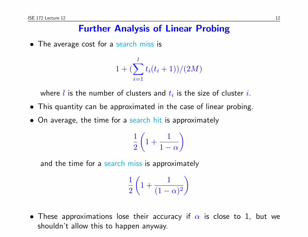
Further Analysis of Linear Probing

• The average cost for a search miss is

1 + (

l∑i=1

ti(ti + 1))/(2M)

where l is the number of clusters and ti is the size of cluster i.

• This quantity can be approximated in the case of linear probing.

• On average, the time for a search hit is approximately

1

2

(1 +

1

1− α

)and the time for a search miss is approximately

1

2

(1 +

1

(1− α)2

)

• These approximations lose their accuracy if α is close to 1, but weshouldn’t allow this to happen anyway.

12


Clustering in Linear Probing

• We have just seen why large clusters are a problem in open addressingschemes.

• Linear probing is particularly susceptible to this problem.

• This is because an empty slot preceded by i full slots has an increasedprobability, (i+ 1)/M , of being filled.

• One way of combating this problem is to use quadratic probing, whichmeans that

h(x, i) = (h′(x) + c1i+ c2i2) mod M, i = 0, . . . ,M − 1

• This alleviates the clustering problem by skipping slots.

• We can choose c1 and c2 such that this sequence generates all possibleaddresses.

13


Double Hashing

• An even better idea is to use double hashing.

• Under a double hashing scheme, we use two hash functions to generatethe sequence as follows.

h(x, i) = (h1(x) + ih2(x)) mod M, i = 0, . . . ,M − 1

• The value of h2(x) must never be zero and should be relatively prime toM for the sequence to include all possible addresses.

• The easiest way to assure this is to choose M to be prime.

• Each pair (h1(x), h2(x)) results in a different sequence, yielding M2

possible sequences, as opposed to M in linear and quadratic probing.

• This results in behavior that is very close to ideal.

• Unfortunately, we can’t delete items by rehashing, as in linear probing.

• To delete, we must use a sentinel.

14


Analyzing Double Hashing

• When collisions are resolved by double hashing, the average time forsearch hits can be approximated by

1

αln

(1

1− α

)and the time for search misses is approximately

1

1− α

• This is a big improvement over linear probing.

• Double hashing allows us to achieve the same performance with a muchsmaller table.

15


Empirical Performance of Open Addressing

Here is a graph showing the time and number of comparisons required toinsert all the words in Dickens’ Tale of Two Cities into a hash table withopen addressing.


Figure 3: Performance of chaining implementation as a function of loadfactor

16


Empirical Performance of Open Addressing (cont.)

• On the previous slide, the blue squares are linear probing and the greentriangles are double hashing.

• The second hash function is a variant of the pseudo-universal one fromLecture 9.

• Note the superior performance of double hasing in terms of requirednumber of comparisons.

• This superior performance does not translate into practical improvementsin running time in this case.

• This may be due to the use of an expensive second hash function.

17


Empirical Performance of Open Addressing

Here is a graph showing the mean and variance of the number of comparisonsrequired to insert each word in the previous experiment.


Figure 4: Performance of open adressing implementations as a function ofload factor

Note here that there is an increase in variance as load factor increases ismuch more dramatic especially with linear probing, as expected.

18


Worst Case Analysis

• So far, we have only looked at average performance over all possibleinputs.

• Particular inputs may not exhibit the nice behavior seen on average.

• As with many algorithms, worst case behavior is easy to find.

• For any hash function, there is always a sequence of inserts that will leadto poor behavior.

• For both open addressing and chaining, a sequence of n inserts couldrequire θ(n2) steps.

• A common way to protect against worst-case behavior in algorithms isto randomize in case a certain common patern leads to the worst case.

• For this purpose, we can use the universal has functions described inLecture 9.

19


Dynamic Hash Tables

• Dynamic hash tables attempt to overcome the limitations of openaddressing when the number of table items is not known at the outset.

• When the table fills up beyond a certain threshold, we simply allocate anew array and rehash all the existing items.

• This operation is expensive, but it happens infrequently.

• Using a technique called amortized analysis, we can show that the averagecost of each operation is still approximately constant.

• This may be a good option in some situations.

20


Python’s Hash Table Implementation

• Python uses open adressing with a variant of double hashing.

self.mask = newsize - 1

perturb = key_hash

while True:

i = (i << 2) + i + perturb + 1;

entry = self.table[i & self.mask]

if entry.key is None:

return entry if free is None else free

if entry.key is key or \

(entry.hash == key_hash and key == entry.key):

return entry

elif entry.key is dummy and free is None:

free = dummy

perturb >>= PERTURB_SHIFT

• The table size is initially 8 and is increased by a factor of 4 whenver itfills up.

• Deletion is by sentinel.

21

Documents

Algorithms in Systems Engineering ISE 172 Lecture 12