Embed Size (px)
Citation preview
Journal of Machine Learning Research 1 (2013) 1-44 Submitted 6/12; Revised 1/13; Published 00/00
Alleviating Naive Bayes Attribute Independence Assumptionby Attribute Weighting
Nayyar A. Zaidi [email protected] of Information TechnologyMonash University, VIC 3800, Australia.
Jesus Cerquides [email protected], Artificial Intelligence Research InstituteSpanish National Research Council, Campus UAB, 08193 Bellaterra, Spain.
Mark J. Carman [email protected] of Information TechnologyMonash University, VIC 3800, Australia.
Geoffrey I. Webb [email protected]
Faculty of Information Technology
Monash University, VIC 3800, Australia.
Editor: Leslie Pack Kaelbling
Abstract
Despite the simplicity of the Naive Bayes classifier, it has continued to perform wellagainst more sophisticated newcomers and has remained, therefore, of great interest to themachine learning community. Of numerous approaches to refining the naive Bayes classifier,attribute weighting has received less attention than it warrants. Most approaches, perhapsinfluenced by attribute weighting in other machine learning algorithms, use weighting toplace more emphasis on highly predictive attributes than those that are less predictive. Inthis paper, we argue that for naive Bayes attribute weighting should instead be used toalleviate the conditional independence assumption. Based on this premise, we propose aweighted naive Bayes algorithm, called WANBIA, that selects weights to minimize eitherthe negative conditional log likelihood or the mean squared error objective functions. Weperform extensive evaluations and find that WANBIA is a competitive alternative to stateof the art classifiers like Random Forest, Logistic Regression and A1DE.
Keywords: Classification, Naive Bayes, Attribute Independence Assumption, WeightedNaive Bayes Classification.
1. Introduction
Naive Bayes (also known as simple Bayes and Idiot’s Bayes) is an extremely simple andremarkably effective approach to classification learning (Lewis, 1998; Hand and Yu, 2001).It infers the probability of a class label given data using a simplifying assumption that theattributes are independent given the label (Kononenko, 1990; Langley et al., 1992). This as-sumption is motivated by the need to estimate high-dimensional multi-variate probabilitiesfrom the training data. If there is sufficient data present for every possible combination ofattribute values, direct estimation of each relevant multi-variate probability will be reliable.
c©2013 Nayyar A. Zaidi, Jesus Cerquides, Mark J. Carman and Geoffrey I. Webb.
Zaidi, Cerquides, Carman, and Webb
In practice, however, this is not the case and most combinations are either not representedin the training data or not present in sufficient numbers. Naive Bayes circumvents thispredicament by its conditional independence assumption. Surprisingly, it has been shownthat the prediction accuracy of naive Bayes compares very well with other more complexclassifiers such as decision trees, instance-based learning and rule learning, especially whenthe data quantity is small (Hand and Yu, 2001; Cestnik et al., 1987; Domingos and Pazzani,1996; Langley et al., 1992).
In practice, naive Bayes’ attribute independence assumption is often violated, and as aresult its probability estimates are often suboptimal. A large literature addresses approachesto reducing the inaccuracies that result from the conditional independence assumption.Such approaches can be placed into two categories. The first category comprises semi-naiveBayes methods. These methods are aimed at enhancing naive Bayes’ accuracy by relaxingthe assumption of conditional independence between attributes given the class label (Lan-gley and Sage, 1994; Friedman and Goldszmidt, 1996; Zheng et al., 1999; Cerquides andDe Mantaras, 2005; Webb et al., 2005, 2011; Zheng et al., 2012). The second category com-prises attribute weighting methods and has received relatively little attention (Hilden andBjerregaard, 1976; Ferreira et al., 2001; Hall, 2007). There is some evidence that attributeweighting appears to have primarily been viewed as a means of increasing the influenceof highly predictive attributes and discounting attributes that have little predictive value.This is not so much evident from the explicit motivation stated in the prior work, butrather from the manner in which weights have been assigned. For example, weighting bymutual information between an attribute and the class is directly using a measure of howpredictive is each individual attribute (Zhang and Sheng, 2004). In contrast, we argue thatthe primary value of attribute weighting is its capacity to reduce the impact on predictionaccuracy of violations of the assumption of conditional attribute independence.
Contributions of this paper are two-fold:
• This paper reviews the state of the art in weighted naive Bayesian classification. Weprovide a compact survey of existing techniques and compare them using the bias-variance decomposition method of Kohavi and Wolpert (1996). We also use Friedmantest and Nemenyi statistics to analyze error, bias, variance and root mean square error.
• We present novel algorithms for learning attribute weights for naive Bayes. It shouldbe noted that the motivation of our work differs from most previous attribute weight-ing methods. We view weighting as a way to reduce the effects of the violations ofthe attribute independence assumption on which naive Bayes is based. Also, ourwork differs from semi-naive Bayes methods, as we weight the attributes rather thanmodifying the structure of naive Bayes.
We propose a weighted naive Bayes algorithm, Weighting attributes to Alleviate NaiveBayes’ Independence Assumption (WANBIA), that introduces weights in naive Bayes andlearns these weights in a discriminative fashion that is minimizing either the negative condi-tional log likelihood or the mean squared error objective functions. Naive Bayes probabilitiesare set to be their maximum a posteriori (MAP) estimates.
The paper is organized as follows: we provide a formal description of the weightednaive Bayes model in section 2. Section 3 provides a survey of related approaches. Our
2
Alleviating NB Attribute Independence Assumption by Attribute Weighting
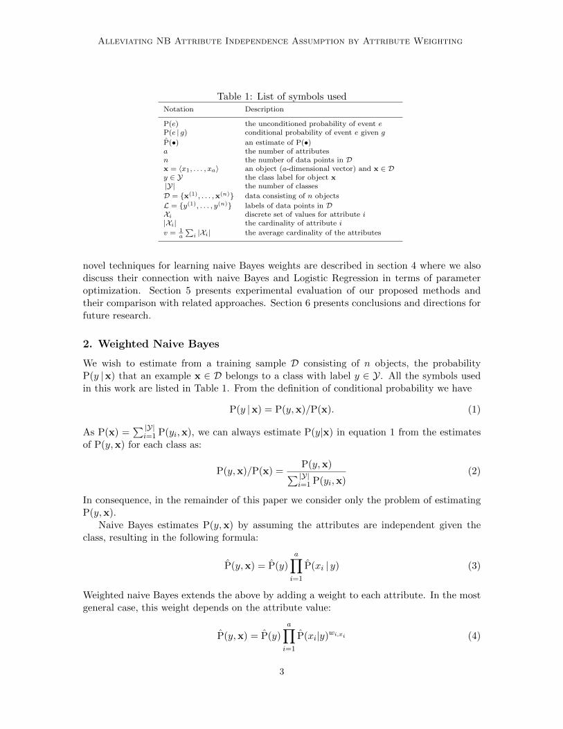
Table 1: List of symbols usedNotation Description
P(e) the unconditioned probability of event eP(e | g) conditional probability of event e given g
P(•) an estimate of P(•)a the number of attributesn the number of data points in Dx = 〈x1, . . . , xa〉 an object (a-dimensional vector) and x ∈ Dy ∈ Y the class label for object x|Y| the number of classes
D = {x(1), . . . ,x(n)} data consisting of n objects
L = {y(1), . . . , y(n)} labels of data points in DXi discrete set of values for attribute i|Xi| the cardinality of attribute i
v = 1a
∑i |Xi| the average cardinality of the attributes
novel techniques for learning naive Bayes weights are described in section 4 where we alsodiscuss their connection with naive Bayes and Logistic Regression in terms of parameteroptimization. Section 5 presents experimental evaluation of our proposed methods andtheir comparison with related approaches. Section 6 presents conclusions and directions forfuture research.
2. Weighted Naive Bayes
We wish to estimate from a training sample D consisting of n objects, the probabilityP(y |x) that an example x ∈ D belongs to a class with label y ∈ Y. All the symbols usedin this work are listed in Table 1. From the definition of conditional probability we have
P(y |x) = P(y,x)/P(x). (1)
As P(x) =∑ |Y|
i=1 P(yi,x), we can always estimate P(y|x) in equation 1 from the estimatesof P(y,x) for each class as:
P(y,x)/P(x) =P(y,x)∑ |Y|i=1 P(yi,x)
(2)
In consequence, in the remainder of this paper we consider only the problem of estimatingP(y,x).
Naive Bayes estimates P(y,x) by assuming the attributes are independent given theclass, resulting in the following formula:
P(y,x) = P(y)
a∏i=1
P(xi | y) (3)
Weighted naive Bayes extends the above by adding a weight to each attribute. In the mostgeneral case, this weight depends on the attribute value:
P(y,x) = P(y)a∏i=1
P(xi|y)wi,xi (4)
3
Zaidi, Cerquides, Carman, and Webb
Doing this results in∑a
i |Xi| weight parameters (and is in some cases equivalent to a “bi-narized logistic regression model” see section 4 for a discussion). A second possibility is togive a single weight per attribute:
P(y,x) = P(y)a∏i=1
P(xi | y)wi (5)
One final possibility is to set all weights to a single value:
P(y,x) = P(y)
(a∏i=1
P(xi | y)
)w(6)
Equation 5 is a special case of equation 4, where ∀i,j wij =wi, and equation 6 is a specialcase of equation 5 where ∀i wi =w. Unless explicitly stated, in this paper we intend theintermediate form when we refer to attribute weighting, as we believe it provides an effectivetrade-off between computational complexity and inductive power.
Appropriate weights can reduce the error that results from violations of naive Bayes’conditional attribute independence assumption. Trivially, if data include a set of a at-tributes that are identical to one another, the error due to the violation of the conditionalindependence assumption can be removed by assigning weights that sum to 1.0 to the setof attributes in the set. For example, the weight for one of the attributes, xi could be setto 1.0, and that of the remaining attributes that are identical to xi set to 0.0. This isequivalent to deleting the remaining attributes. Note that, any assignment of weights suchthat their sum is 1.0 for the a attributes will have the same effect, for example, we couldset the weights of all a attributes to 1/a.
Attribute weighting is strictly more powerful than attribute selection, as it is possible toobtain identical results to attribute selection by setting the weights of selected attributes to1.0 and of discarded attributes to 0.0, and assignment of other weights can create classifiersthat cannot be expressed using attribute selection.
2.1 Dealing with Dependent Attributes by Weighting: A Simple Example
This example shows the relative performance of naive Bayes and weighted naive Bayesas we vary the conditional dependence between attributes. In particular it demonstrateshow optimal assignment of weights will never result in higher error than attribute selectionor standard naive Bayes, and that for certain violations of the attribute independenceassumption it can result in lower error than either.
We will constrain ourselves to a binary class problem with two binary attributes. Wequantify the conditional dependence between the attributes using the Conditional MutualInformation (CMI):
I(X1, X2|Y ) =∑y
∑x2
∑x1
P(x1, x2, y) logP(x1, x2|y)
P(x1|y)P(x2|y)(7)
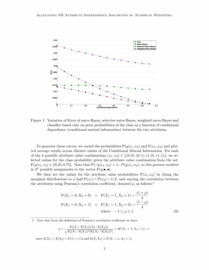
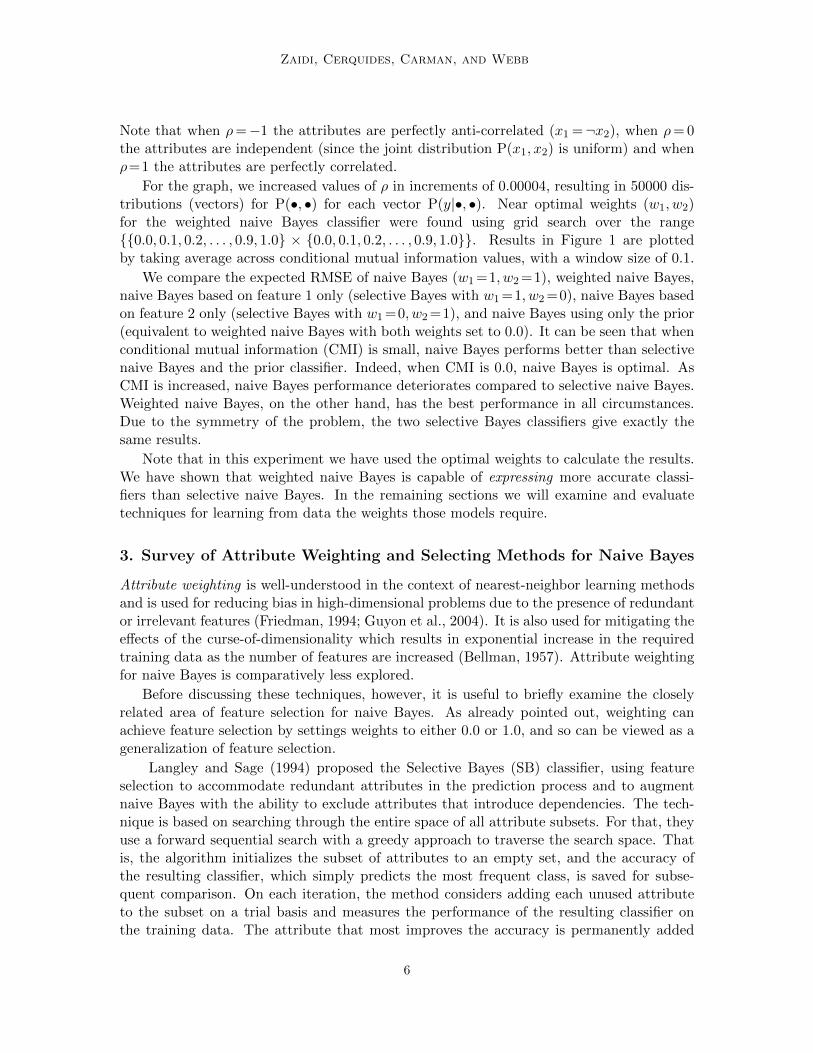
The results of varying the conditional dependence between the attributes on the performanceof the different classifiers in terms of their Root Mean Squared Error (RMSE) is shown inFigure 1.
4
Alleviating NB Attribute Independence Assumption by Attribute Weighting
0 0.1 0.2 0.3 0.4 0.5 0.6 0.70
0.005
0.01
0.015
0.02
0.025
0.03
0.035
0.04
0.045
0.05
Err
or
Conditional Dependence
Prior
Naive Bayes
Selective Naive Bayes
Weighted Naive Bayes
Figure 1: Variation of Error of naive Bayes, selective naive Bayes, weighted naive Bayes andclassifier based only on prior probabilities of the class as a function of conditionaldependence (conditional mutual information) between the two attributes.
To generate these curves, we varied the probabilities P(y|x1, x2) and P(x1, x2) and plot-ted average results across distinct values of the Conditional Mutual Information. For eachof the 4 possible attribute value combinations (x1, x2) ∈ {(0, 0), (0, 1), (1, 0), (1, 1)}, we se-lected values for the class probability given the attribute value combination from the set:P(y|x1, x2) ∈ {0.25, 0.75}. Note that P(¬y|x1, x2) = 1−P (y|x1, x2), so this process resultedin 24 possible assignments to the vector P(y|•, •).
We then set the values for the attribute value probabilities P(x1, x2) by fixing themarginal distributions to a half P(x1) = P(x2) = 1/2, and varying the correlation betweenthe attributes using Pearson’s correlation coefficient, denoted ρ, as follows:1
P(X1 = 0, X2 = 0) = P(X1 = 1, X2 = 1) =(1 + ρ)
4
P(X1 = 0, X2 = 1) = P(X1 = 1, X2 = 0) =(1− ρ)
4where − 1 ≤ ρ ≤ 1 (8)
1. Note that from the definition of Pearson’s correlation coefficient we have:
ρ =E[(X1−E[X1])(X2−E[X2])]√
E[(X1−E[X1])2]E[(X2−E[X2])2]= 4P(X1 = 1, X2 = 1)−1
since E[X1] = E[X2] = P(1) = 1/2 and E[X1X2] = P(X1 = 1, X2 = 1)
5
Zaidi, Cerquides, Carman, and Webb
Note that when ρ=−1 the attributes are perfectly anti-correlated (x1 =¬x2), when ρ= 0the attributes are independent (since the joint distribution P(x1, x2) is uniform) and whenρ=1 the attributes are perfectly correlated.
For the graph, we increased values of ρ in increments of 0.00004, resulting in 50000 dis-tributions (vectors) for P(•, •) for each vector P(y|•, •). Near optimal weights (w1, w2)for the weighted naive Bayes classifier were found using grid search over the range{{0.0, 0.1, 0.2, . . . , 0.9, 1.0} × {0.0, 0.1, 0.2, . . . , 0.9, 1.0}}. Results in Figure 1 are plottedby taking average across conditional mutual information values, with a window size of 0.1.
We compare the expected RMSE of naive Bayes (w1 =1, w2 =1), weighted naive Bayes,naive Bayes based on feature 1 only (selective Bayes with w1 =1, w2 =0), naive Bayes basedon feature 2 only (selective Bayes with w1 =0, w2 =1), and naive Bayes using only the prior(equivalent to weighted naive Bayes with both weights set to 0.0). It can be seen that whenconditional mutual information (CMI) is small, naive Bayes performs better than selectivenaive Bayes and the prior classifier. Indeed, when CMI is 0.0, naive Bayes is optimal. AsCMI is increased, naive Bayes performance deteriorates compared to selective naive Bayes.Weighted naive Bayes, on the other hand, has the best performance in all circumstances.Due to the symmetry of the problem, the two selective Bayes classifiers give exactly thesame results.
Note that in this experiment we have used the optimal weights to calculate the results.We have shown that weighted naive Bayes is capable of expressing more accurate classi-fiers than selective naive Bayes. In the remaining sections we will examine and evaluatetechniques for learning from data the weights those models require.
3. Survey of Attribute Weighting and Selecting Methods for Naive Bayes
Attribute weighting is well-understood in the context of nearest-neighbor learning methodsand is used for reducing bias in high-dimensional problems due to the presence of redundantor irrelevant features (Friedman, 1994; Guyon et al., 2004). It is also used for mitigating theeffects of the curse-of-dimensionality which results in exponential increase in the requiredtraining data as the number of features are increased (Bellman, 1957). Attribute weightingfor naive Bayes is comparatively less explored.
Before discussing these techniques, however, it is useful to briefly examine the closelyrelated area of feature selection for naive Bayes. As already pointed out, weighting canachieve feature selection by settings weights to either 0.0 or 1.0, and so can be viewed as ageneralization of feature selection.
Langley and Sage (1994) proposed the Selective Bayes (SB) classifier, using featureselection to accommodate redundant attributes in the prediction process and to augmentnaive Bayes with the ability to exclude attributes that introduce dependencies. The tech-nique is based on searching through the entire space of all attribute subsets. For that, theyuse a forward sequential search with a greedy approach to traverse the search space. Thatis, the algorithm initializes the subset of attributes to an empty set, and the accuracy ofthe resulting classifier, which simply predicts the most frequent class, is saved for subse-quent comparison. On each iteration, the method considers adding each unused attributeto the subset on a trial basis and measures the performance of the resulting classifier onthe training data. The attribute that most improves the accuracy is permanently added
6
Alleviating NB Attribute Independence Assumption by Attribute Weighting
to the subset. The algorithm terminates when addition of any attribute results in reducedaccuracy, at which point it returns the list of current attributes along with their ranks. Therank of the attribute is based on the order in which they are added to the subset.
Similar to Langley and Sage (1994), Correlation-based Feature Selection (CFS) used acorrelation measure as a metric to determine the relevance of the attribute subset (Hall,2000). It uses a best-first search to traverse through feature subset space. Like SB, it startswith an empty set and generates all possible single feature expansions. The subset withhighest evaluation is selected and expanded in the same manner by adding single features.If expanding a subset results in no improvement, the search drops back to the next bestunexpanded subset and continues from there. The best subset found is returned whenthe search terminates. CFS uses a stopping criterion of five consecutive fully expandednon-improving subsets.
There has been a growing trend in the use of decision trees to improve the performanceof other learning algorithms and naive Bayes classifiers are no exception. For example, onecan build a naive Bayes classifier by using only those attributes appearing in a C4.5 decisiontree. This is equivalent to giving zero weights to attributes not appearing in the decisiontree. The Selective Bayesian Classifier (SBC) of Ratanamahatana and Gunopulos (2003)also employs decision trees for attribute selection for naive Bayes. Only those attributesappearing in the top three levels of a decision tree are selected for inclusion in naive Bayes.Since decision trees are inherently unstable, five decision trees (C4.5) are generated onsamples generated by bootstrapping 10% from the training data. Naive Bayes is trained onan attribute set which comprises the union of attributes appearing in all five decision trees.
One of the earliest works on weighted naive Bayes is by Hilden and Bjerregaard (1976),who used weighting of the form of equation 6. This strategy uses a single weight andtherefore is not strictly performing attribute weighting. Their approach is motivated asa means of alleviating the effects of violations of the attribute independence assumption.Setting w to unity is appropriate when the conditional independence assumption is satisfied.However, on their dataset (acute abdominal pain study in Copenhagen by Bjerregaard et al.(1976)), improved classification was obtained when w was small, with an optimum valueas low as 0.3. The authors point out that if symptom variables of a clinical field trial arenot independent, but pair-wise correlated with independence between pairs, then w = 0.5will be the correct choice since using w = 1 would make all probabilities the square of whatthey ought be. Looking at the optimal value of w = 0.3 for their dataset, they suggestedthat out of ten symptoms, only three are providing independent information. The value ofw was obtained by maximizing the log-likelihood over the entire testing sample.
Zhang and Sheng (2004) used the gain ratio of an attribute with the class labels as itsweight. Their formula is shown in equation 9. The gain ratio is a well-studied attributeweighting technique and is generally used for splitting nodes in decision trees (Duda et al.,2006). The weight of each attribute is set to the gain ratio of the attribute relative to theaverage gain ratio across all attributes. Note that, as a result of the definition at least one(possibly many) of the attributes have weights greater than 1, which means that they arenot only attempting to lessen the effects of the independence assumption – otherwise theywould restrict the weights to be no more than one.
wi =GR(i)
1a
∑ai=1 GR(i)
(9)
7
Zaidi, Cerquides, Carman, and Webb
The gain ratio of an attribute is then simply the Mutual Information between that attributeand the class label divided by the entropy of that attribute:
GR(i) =I(Xi, Y )
H(Xi)=
∑y
∑x1
P(x1, y) log P(x1,y)P(x1)P(y)∑
x1P(x1) log 1
P(x1)
(10)
Several other wrapper-based methods are also proposed in Zhang and Sheng (2004). Forexample, they use a simple hill climbing search to optimize weight w using Area Under Curve(AUC) as an evaluation metric. Another Markov-Chain-Monte-Carlo (MCMC) method isalso proposed.
An attribute weighting scheme based on differential evolution algorithms for naive Bayesclassification have been proposed in Wu and Cai (2011). First, a population of attributeweight vectors is randomly generated, weights in the population are constrained to bebetween 0 and 1. Second, typical genetic algorithmic steps of mutation and cross-overare performed over the the population. They defined a fitness function which is used todetermine if mutation can replace the current individual (weight vector) with a new one.Their algorithm employs a greedy search strategy, where mutated individuals are selectedas offspring only if the fitness is better than that of target individual. Otherwise, the targetis maintained in the next iteration.
A scheme used in Hall (2007) is similar in spirit to SBC where the weight assignedto each attribute is inversely proportional to the minimum depth at which they were firsttested in an unpruned decision tree. Weights are stabilized by averaging across 10 decisiontrees learned on data samples generated by bootstrapping 50% from the training data.Attributes not appearing in the decision trees are assigned a weight of zero. For example,one can assign weight to an attribute i as:
wi =1
T
T∑t
1√dti
(11)
where dti is the minimum depth at which the attribute i appears in decision tree t, and Tis the total number of decision trees generated. To understand whether the improvementin naive Bayes accuracy was due to attribute weighting or selection, a variant of the aboveapproach was also proposed where all non-zero weights are set to one. This is equivalent toSBC except using a bootstrap size of 50% with 10 iterations.
Both SB and CFS are feature selection methods. Since selecting an optimal numberof features is not trivial, Hall (2007) proposed to use SB and CFS for feature weighting innaive Bayes. For example, the weight of an attribute i can be defined as:
wi =1√ri
(12)
where ri is the rank of the feature based on SB and CFS feature selection.The feature weighting method proposed in Ferreira et al. (2001) is the only one to use
equation 4, weighting each attribute value rather than each attribute. They used entropy-based discretization for numeric attributes and assigned a weight to each partition (value)of the attribute that is proportional to its predictive capability of the class. Different
8
Alleviating NB Attribute Independence Assumption by Attribute Weighting
weight functions are proposed to assign weights to the values. These functions measure thedifference between the distribution over classes for the particular attribute-value pair and a“baseline class distribution”. The choice of weight function reduces to a choice of baselinedistribution and the choice of measure quantifying the difference between the distributions.They used two simple baseline distribution schemes. The first assumes equiprobable classes,i.e. uniform class priors. In that case the weight of for value j of the attribute i can bewritten as:
wij ∝
(∑y
|P(y|Xi=j)− 1
|Y|| α)1/α
(13)
where P(y|Xi = j) denotes the probability that the class is y given that the i-th attributeof a data point has value j. Alternatively, the baseline class distribution can be set to theclass probabilities across all values of the attribute (i.e. the class priors). The weighingfunction will take the form:
wij ∝
(∑y
|P(y|Xi=j)− P(y|Xi 6=miss) | α)1/α
(14)
where P(y|Xi 6= miss) is the class prior probability across all data points for which theattribute i is not missing. Equation 13 and 14 assume an Lα distance metric where α = 2corresponds to the L2 norm. Similarly, they have also proposed to use distance based onKullback-Leibler divergence between the two distributions to set weights.
Many researchers have investigated techniques for extending the basic naive Bayes inde-pendence model with a small number of additional dependencies between attributes in orderto improve classification performance (Zheng and Webb, 2000). Popular examples of suchsemi-naive Bayes methods include Tree-Augmented Naive Bayes (TAN) (Friedman et al.,1997) and ensemble methods such as Averaged n-Dependence Estimators (AnDE) (Webbet al., 2011). While detailed discussion of these methods is beyond the scope of this work, wewill describe both TAN and AnDE in section 5.10 for the purposes of empirical comparison.
Semi-naive Bayes methods usually limit the structure of the dependency network tosimple structures such as trees, but more general graph structures can also be learnt. Con-siderable research has been done in the area of learning general Bayesian Networks (Greineret al., 2004; Grossman and Domingos, 2004; Roos et al., 2005), with techniques differing onwhether the network structure is chosen to optimize a generative or discriminative objectivefunction, and whether the same objective is also used for optimizing the parameters of themodel. Indeed optimizing network structure using a discriminative objective function canquickly become computationally challenging and thus recent work in this area has lookedat efficient heuristics for discriminative structure learning (Pernkopf and Bilmes, 2010) andat developing decomposable discriminative objective functions (Carvalho et al., 2011).
In this paper we are interested in improving performance of the NB classifier by reducingthe effect of attribute independence violations through attribute weighting. We do notattempt to identify the particular dependencies between attributes that cause the violationsand thus are not attempting to address the much harder problem of inducing the dependencynetwork structure. While it is conceivable that semi-naive Bayes methods and more generalBayesian Network classifier learning could also benefit from attribute weighting, we leaveits investigation to future work.
9
Zaidi, Cerquides, Carman, and Webb
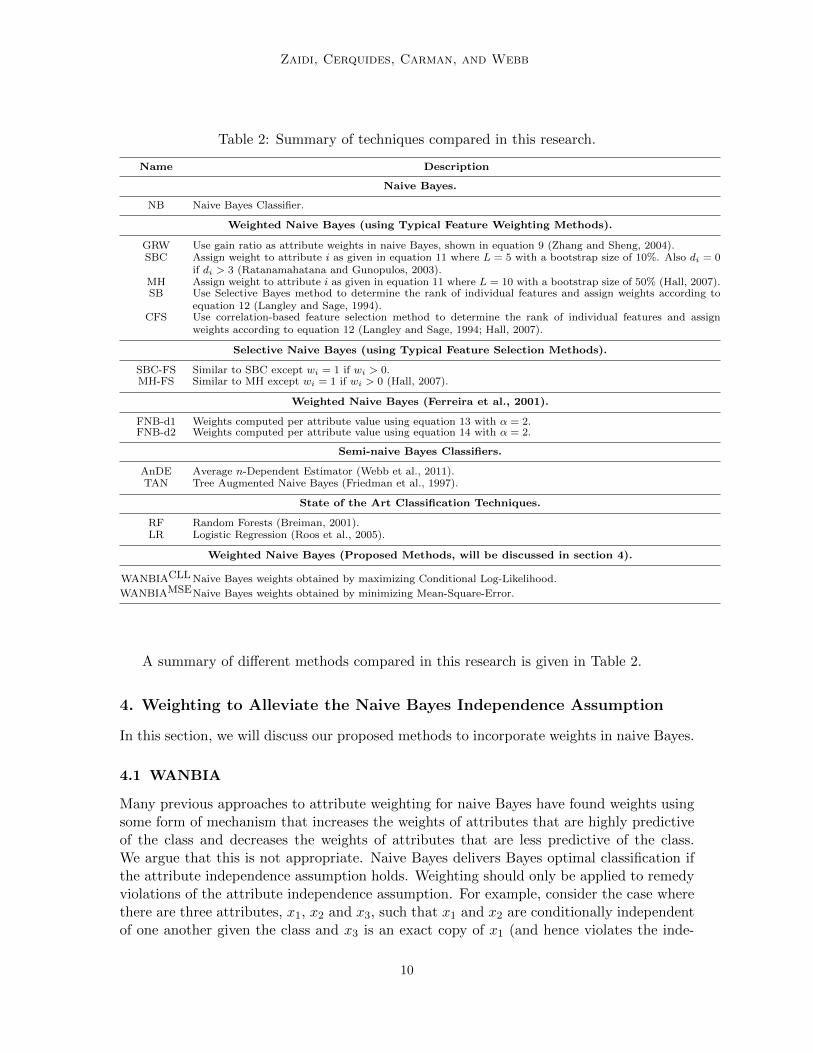
Table 2: Summary of techniques compared in this research.
Name Description
Naive Bayes.
NB Naive Bayes Classifier.
Weighted Naive Bayes (using Typical Feature Weighting Methods).
GRW Use gain ratio as attribute weights in naive Bayes, shown in equation 9 (Zhang and Sheng, 2004).SBC Assign weight to attribute i as given in equation 11 where L = 5 with a bootstrap size of 10%. Also di = 0
if di > 3 (Ratanamahatana and Gunopulos, 2003).MH Assign weight to attribute i as given in equation 11 where L = 10 with a bootstrap size of 50% (Hall, 2007).SB Use Selective Bayes method to determine the rank of individual features and assign weights according to
equation 12 (Langley and Sage, 1994).CFS Use correlation-based feature selection method to determine the rank of individual features and assign
weights according to equation 12 (Langley and Sage, 1994; Hall, 2007).
Selective Naive Bayes (using Typical Feature Selection Methods).
SBC-FS Similar to SBC except wi = 1 if wi > 0.MH-FS Similar to MH except wi = 1 if wi > 0 (Hall, 2007).
Weighted Naive Bayes (Ferreira et al., 2001).
FNB-d1 Weights computed per attribute value using equation 13 with α = 2.FNB-d2 Weights computed per attribute value using equation 14 with α = 2.
Semi-naive Bayes Classifiers.
AnDE Average n-Dependent Estimator (Webb et al., 2011).TAN Tree Augmented Naive Bayes (Friedman et al., 1997).
State of the Art Classification Techniques.
RF Random Forests (Breiman, 2001).LR Logistic Regression (Roos et al., 2005).
Weighted Naive Bayes (Proposed Methods, will be discussed in section 4).
WANBIACLL Naive Bayes weights obtained by maximizing Conditional Log-Likelihood.
WANBIAMSENaive Bayes weights obtained by minimizing Mean-Square-Error.
A summary of different methods compared in this research is given in Table 2.
4. Weighting to Alleviate the Naive Bayes Independence Assumption
In this section, we will discuss our proposed methods to incorporate weights in naive Bayes.
4.1 WANBIA
Many previous approaches to attribute weighting for naive Bayes have found weights usingsome form of mechanism that increases the weights of attributes that are highly predictiveof the class and decreases the weights of attributes that are less predictive of the class.We argue that this is not appropriate. Naive Bayes delivers Bayes optimal classification ifthe attribute independence assumption holds. Weighting should only be applied to remedyviolations of the attribute independence assumption. For example, consider the case wherethere are three attributes, x1, x2 and x3, such that x1 and x2 are conditionally independentof one another given the class and x3 is an exact copy of x1 (and hence violates the inde-
10
Alleviating NB Attribute Independence Assumption by Attribute Weighting
pendence assumption). Irrespective of any measure of how well these three attributes eachpredict the class, Bayes optimal classification will be obtained by setting the weights of x1
and x3 to sum to 1.0 and setting the weight of x2 to 1.0. In contrast, a method that uses ameasure such as mutual information with the class to weight the attribute will reduce theaccuracy of the classifier relative to using uniform weights in any situation where x1 and x3
receive higher weights than x2.
Rather than selecting weights based on measures of predictiveness, we suggest it is moreprofitable to pursue approaches such as those of Zhang and Sheng (2004); Wu and Cai(2011) that optimize the weights to improve the prediction performance of the weightedclassifier as a whole.
Following from equations 1, 2 and 5, let us re-define the weighted naive Bayes model as:
P(y|x;π,Θ,w) =πy∏i θwi
Xi=xi|y∑y′ πy′
∏i θwi
Xi=xi|y′(15)
with constraints: ∑y πy=1 and ∀y,i
∑j θXi=xi|y=1 (16)
where
• {πy, θXi=xi|y} are naive Bayes parameters.
• π ∈ [0, 1] |Y| is a class probability vector.
• The matrix Θ consist of class and attribute-dependent probability vectors θi,y ∈[0, 1] | Xi | .
• w is a vector of class-independent weights, wi for each attribute i.
Our proposed method WANBIA is inspired by Cerquides and Mantaras (2005) whereweights of different classifiers in an ensemble are calculated by maximizing the conditionallog-likelihood (CLL) of the data. We will follow their approach of maximizing the CLL ofthe data to determine weights w in the model. In doing so, we will make the followingassumptions:
• Naive Bayes parameters (πy, θXi=xi|y) are fixed. Hence we can write P(y|x;π,Θ,w)
in equation 15 as P(y|x; w).
• Weights lie in the interval between zero and one and hence w ∈ [0, 1]a.
For notational simplicity, we will write conditional probabilities as θxi|y instead of θXi=xi|y.Since our prior is constant, let us define our supervised posterior as follows:
P(L |D,w) =
| D |∏j=1
P(y(j)|x(j); w) (17)
11
Zaidi, Cerquides, Carman, and Webb
Taking the log of equation 17, we get the Conditional Log-Likelihood (CLL) function, soour objective function can be defined as:
CLL(w) = log P(L |D,w) (18)
=
| D |∑j=1
log P(y(j)|x(j); w) (19)
=
| D |∑j=1
logγyx(w)∑y′ γy′x(w)
(20)
where
γyx(w) = πy∏i
θwi
xi|y (21)
The proposed method WANBIACLL is aimed at solving the following optimization problem:find the weights w that maximizes the objective function CLL(w) in equation 18 subjectto 0 ≤ wi ≤ 1 ∀i. We can solve the problem by using the L-BFGS-M optimizationprocedure (C. Zhu and Nocedal, 1997). In order to do that, we need to be able to assessCLL(w) in equation 18 and its gradient.
Before calculating the gradient of CLL(w) with respect to w, let us find out the gradientof γyx(w) with respect to wi, we can write:
∂
∂wiγyx(w) = (πy
∏i′ 6=i
θwi′xi′ |y
)∂
∂wiθwi
xi|y
= (πy∏i′ 6=i
θwi′xi′ |y
) θwi
xi|y log(θxi|y)
= γyx(w) log(θxi|y) (22)
Now, we can write the gradient of CLL(w) as:
∂
∂wiCLL(w) =
∂
∂wi
∑x∈D
log(γyx(w))− log(∑y′
γy′x(w))
(23)
=∑x∈D
(γyx(w) log(θxi|y)
γyx(w)−∑
y′ γy′x(w) log(θxi|y′)∑y′ γy′x(w)
)
=∑x∈D
log(θxi|y)−∑y′
P(y′|x; w) log(θxi|y′)
(24)
WANBIACLL evaluates the function in equation 18 and its gradient in equation 23 todetermine optimal values of weight vector w.
Instead of maximizing the supervised posterior, one can also minimize Mean Square
Error (MSE). Our second proposed weighting scheme WANBIAMSE is based on minimizing
12
Alleviating NB Attribute Independence Assumption by Attribute Weighting
the MSE function. Based on MSE, we can define our objective function as follows:
MSE(w) =1
2
∑x(j)∈D
∑y
(P(y|x(j))− P(y|x(j)))2 (25)
where we define
P(y|x(j)) =
{1 if y = y(j)
0 otherwise(26)
The gradient of MSE(w) in equation 25 with respect to w can be derived as:
∂MSE(w)
∂wi= −
∑x∈D
∑y
(P(y|x)−P(y|x)
) ∂P(y|x)
∂wi(27)
where
∂P(y|x)
∂wi=
∂∂wi
γyx(w)∑y′ γy′x(w)
−γyx(w) ∂
∂wi
∑y′ γy′x(w)
(∑
y′ γy′x(w))2
=1∑
y′ γy′x(w)
∂γyx(w)
∂wi− P(y|x)
∑y′
∂γy′x(w)
∂wi
Following from equation 22, we can write:
∂P(y|x)
∂wi=
1∑y′ γy′x(w)
γyx(w) log(θxi|y)− P(y|x)∑y′
γy′x(w) log(θxi|y′)
= P(y|x) log(θxi|y)− P(y|x)
∑y′
P(y′|x) log(θxi|y′)
= P(y|x)
log(θxi|y)−∑y′
P(y′|x) log(θxi|y′)
(28)
Plugging the value of ∂P(y|x)∂wi
from equation 28 in equation 27, we can write the gradient as:
∂MSE(w)
∂wi= −
∑x∈D
∑y
(P(y|x)− P(y|x)
)P(y|x)log(θxi|y)−
∑y′
P(y′|x) log(θxi|y′)
(29)
WANBIAMSE evaluates the function in equation 25 and its gradient in equation 29 todetermine the optimal value of weight vector w.
4.2 Connections with Logistic Regression
In this section, we will re-visit naive Bayes to illustrate WANBIA’s connection with thelogistic regression.
13
Zaidi, Cerquides, Carman, and Webb
4.2.1 Background: Naive Bayes and Logistic Regression
As discussed in section 2 and 4.1, the naive Bayes (NB) model for estimating P(y|x) isparameterized by a class probability vector π ∈ [0, 1] |Y| and a matrix Θ, consisting of classand attribute dependent probability vectors θi,y ∈ [0, 1]|Xi|. The NB model thus contains
( |Y| − 1) + |Y|∑i
(|Xi| − 1) (30)
free parameters, which are estimated by maximizing the likelihood function:
P(D,L;π,Θ) =∏j
P(y(j),x(j)) (31)
or the posterior over model parameters (in which case they are referred to as maximum aposteriori or MAP estimates). Importantly, these estimates can be calculated analyticallyfrom attribute-value count vectors.
Meanwhile a multi-class logistic regression model is parameterized by a vector α ∈ R |Y|and matrix B ∈ R |Y|×a each consisting of real values, and can be written as:
PLR(y|x;α,B) =exp(αy +
∑i βi,yxi)∑
y′ exp(αy′ +∑
i βi,y′xi)(32)
where
α1 =0 & ∀i βi,1 =0 (33)
The constraints arbitrarily setting all parameters for y= 1 to the value zero are necessaryonly to prevent over-parameterization. The LR model, therefore, has:
( |Y| − 1)× (1 + a) (34)
free parameters. Rather than maximizing the likelihood, LR parameters are estimated bymaximizing the conditional likelihood of the class labels given the data:
P(L|D;α,B) =∏j
P(y(j)|x(j)) (35)
or the corresponding posterior distribution. Estimating the parameters in this fashionrequires search using gradient-based methods.
Mathematically the relationship between the two models is simple. One can comparethe models, by considering that the “multiplicative contribution” of an attribute value xiin NB is found by simply looking up the corresponding parameter θXi=xi|y in Θ, while forLR it is calculated as exp(βi,yxi), i.e. by taking the exponent of the product of the valuewith an attribute (but not value) dependent parameter βi,y from B.2
2. Note that unlike the NB model, the LR model does not require that the domain of attribute values bediscrete. Non-discrete data can also be handled by Naive Bayes models, but a different parameterizationfor the distribution over attribute values must be used.
14
Alleviating NB Attribute Independence Assumption by Attribute Weighting
4.2.2 Parameters of Weighted Attribute Naive Bayes
The WANBIA model is an extension of the NB model where we introduce a weight vectorw ∈ [0, 1]a containing a class-independent weight wi for each attribute i. The model aswritten in equation 15 includes the NB model as a special case (where w = 1). We donot treat the NB parameters of the model as free however, but instead fix them to theirMAP estimates (assuming the weights were all one), which can be computed analyticallyand therefore does not require any search. We then estimate the parameter vector w bymaximizing the Conditional Log Likelihood (CLL) or by minimizing the Mean SquaredError (MSE).3
Thus in terms of the number of parameters that needs to be estimated using gradient-based search, a WANBIA model can be considered to have a free parameters, which isalways less than the corresponding LR model with ( |Y| − 1)(1 + a) free parameters to beestimated. Thus for a binary class problems containing only binary attributes, WANBIAhas 1 less free parameter than LR, but for multi-class problems with binary attributes itresults in a multiplicative factor of |Y| − 1 fewer parameters. Since parameter estimationusing CLL or MSE (or even Hinge Loss) requires search, fewer free parameters to estimatemeans faster learning and therefore scaling to larger problems.
For problems containing non-binary attributes, WANBIA allows us to build (more ex-pressive) non-linear classifiers, which are not possible for Logistic Regression unless one“binarizes” all attributes, with the resulting blow-out in the number of free parameters asmentioned above. One should note that LR can only operate on nominal data by bina-rizing it. Therefore, on discrete problems with nominal data, WANBIA offers significantadvantage in terms of the number of free parameters.
Lest the reader assume that the only goal of this work is to find a more computationallyefficient version of LR, we note that the real advantage of the WANBIA model is to makeuse of the information present in the easy to compute naive Bayes MAP estimates to guidethe search toward reasonable settings for parameters of a model that is not hampered by theassumption of attribute independence.
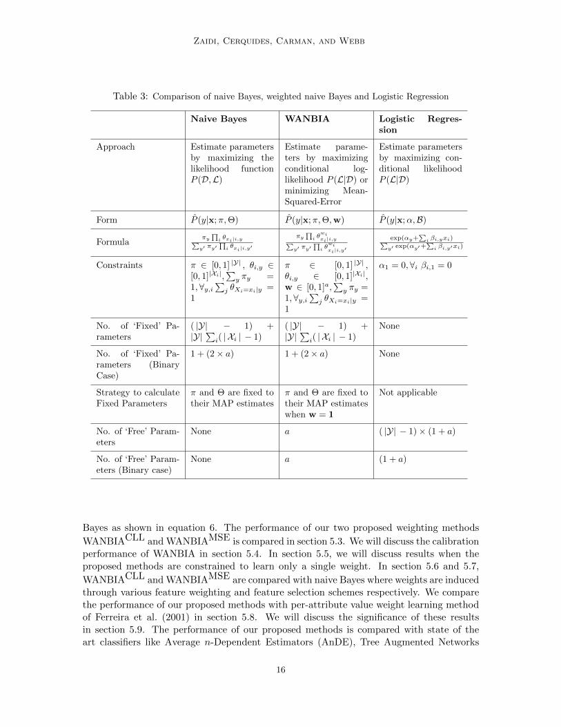
A summary of the comparison of naive Bayes, WANBIA and Logistic Regression is givenin Table 3.
5. Experiments
In this section, we compare the performance of our proposed methods WANBIACLL and
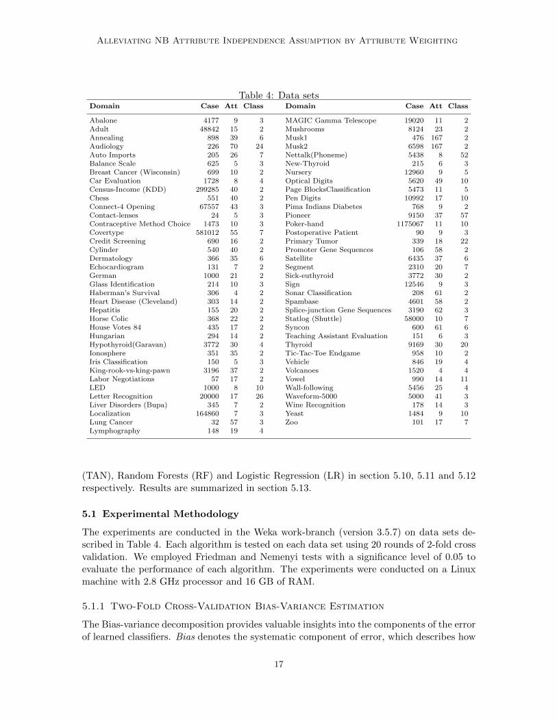
WANBIAMSE with state of the art classifiers, existing semi-naive Bayes methods andweighted naive Bayes methods based on both attribute selection and attribute weighting.The performance is analyzed in terms of 0-1 loss, root mean square error (RMSE), bias andvariance on 73 natural domains from the UCI repository of machine learning (Frank andAsuncion, 2010). Table 4 describes the details of each data set used, including the numberof instances, attributes and classes.
This section is organized as follows: we will discuss our experimental methodologywith details on statistics employed and miscellaneous issues in section 5.1. Section 5.2illustrates the impact of a single weight on bias, variance, 0-1 loss and RMSE of naive
3. Note that we cannot maximize the Log Likelihood (LL) since the model is not generative.
15
Zaidi, Cerquides, Carman, and Webb
Table 3: Comparison of naive Bayes, weighted naive Bayes and Logistic Regression
Naive Bayes WANBIA Logistic Regres-sion
Approach Estimate parametersby maximizing thelikelihood functionP (D,L)
Estimate parame-ters by maximizingconditional log-likelihood P (L|D) orminimizing Mean-Squared-Error
Estimate parametersby maximizing con-ditional likelihoodP (L|D)
Form P (y|x;π,Θ) P (y|x;π,Θ,w) P (y|x;α,B)
Formulaπy
∏i θxi|i,y∑
y′ πy′∏
i θxi|i,y′
πy∏
i θwixi|i,y∑
y′ πy′∏
i θwixi|i,y′
exp(αy+∑
i βi,yxi)∑y′ exp(αy′+
∑i βi,y′xi)
Constraints π ∈ [0, 1] |Y| , θi,y ∈[0, 1]|Xi|,
∑y πy =
1,∀y,i∑j θXi=xi|y =
1
π ∈ [0, 1] |Y| ,θi,y ∈ [0, 1]|Xi|,w ∈ [0, 1]a,
∑y πy =
1,∀y,i∑j θXi=xi|y =
1
α1 = 0,∀i βi,1 = 0
No. of ‘Fixed’ Pa-rameters
( |Y| − 1) +|Y|
∑i( | Xi | − 1)
( |Y| − 1) +|Y|
∑i( | Xi | − 1)
None
No. of ‘Fixed’ Pa-rameters (BinaryCase)
1 + (2× a) 1 + (2× a) None
Strategy to calculateFixed Parameters
π and Θ are fixed totheir MAP estimates
π and Θ are fixed totheir MAP estimateswhen w = 1
Not applicable
No. of ‘Free’ Param-eters
None a ( |Y| − 1)× (1 + a)
No. of ‘Free’ Param-eters (Binary case)
None a (1 + a)
Bayes as shown in equation 6. The performance of our two proposed weighting methods
WANBIACLL and WANBIAMSE is compared in section 5.3. We will discuss the calibrationperformance of WANBIA in section 5.4. In section 5.5, we will discuss results when theproposed methods are constrained to learn only a single weight. In section 5.6 and 5.7,
WANBIACLL and WANBIAMSE are compared with naive Bayes where weights are inducedthrough various feature weighting and feature selection schemes respectively. We comparethe performance of our proposed methods with per-attribute value weight learning methodof Ferreira et al. (2001) in section 5.8. We will discuss the significance of these resultsin section 5.9. The performance of our proposed methods is compared with state of theart classifiers like Average n-Dependent Estimators (AnDE), Tree Augmented Networks
16
Alleviating NB Attribute Independence Assumption by Attribute Weighting
Table 4: Data setsDomain Case Att Class Domain Case Att Class
Abalone 4177 9 3 MAGIC Gamma Telescope 19020 11 2Adult 48842 15 2 Mushrooms 8124 23 2Annealing 898 39 6 Musk1 476 167 2Audiology 226 70 24 Musk2 6598 167 2Auto Imports 205 26 7 Nettalk(Phoneme) 5438 8 52Balance Scale 625 5 3 New-Thyroid 215 6 3Breast Cancer (Wisconsin) 699 10 2 Nursery 12960 9 5Car Evaluation 1728 8 4 Optical Digits 5620 49 10Census-Income (KDD) 299285 40 2 Page BlocksClassification 5473 11 5Chess 551 40 2 Pen Digits 10992 17 10Connect-4 Opening 67557 43 3 Pima Indians Diabetes 768 9 2Contact-lenses 24 5 3 Pioneer 9150 37 57Contraceptive Method Choice 1473 10 3 Poker-hand 1175067 11 10Covertype 581012 55 7 Postoperative Patient 90 9 3Credit Screening 690 16 2 Primary Tumor 339 18 22Cylinder 540 40 2 Promoter Gene Sequences 106 58 2Dermatology 366 35 6 Satellite 6435 37 6Echocardiogram 131 7 2 Segment 2310 20 7German 1000 21 2 Sick-euthyroid 3772 30 2Glass Identification 214 10 3 Sign 12546 9 3Haberman’s Survival 306 4 2 Sonar Classification 208 61 2Heart Disease (Cleveland) 303 14 2 Spambase 4601 58 2Hepatitis 155 20 2 Splice-junction Gene Sequences 3190 62 3Horse Colic 368 22 2 Statlog (Shuttle) 58000 10 7House Votes 84 435 17 2 Syncon 600 61 6Hungarian 294 14 2 Teaching Assistant Evaluation 151 6 3Hypothyroid(Garavan) 3772 30 4 Thyroid 9169 30 20Ionosphere 351 35 2 Tic-Tac-Toe Endgame 958 10 2Iris Classification 150 5 3 Vehicle 846 19 4King-rook-vs-king-pawn 3196 37 2 Volcanoes 1520 4 4Labor Negotiations 57 17 2 Vowel 990 14 11LED 1000 8 10 Wall-following 5456 25 4Letter Recognition 20000 17 26 Waveform-5000 5000 41 3Liver Disorders (Bupa) 345 7 2 Wine Recognition 178 14 3Localization 164860 7 3 Yeast 1484 9 10Lung Cancer 32 57 3 Zoo 101 17 7Lymphography 148 19 4
(TAN), Random Forests (RF) and Logistic Regression (LR) in section 5.10, 5.11 and 5.12respectively. Results are summarized in section 5.13.
5.1 Experimental Methodology
The experiments are conducted in the Weka work-branch (version 3.5.7) on data sets de-scribed in Table 4. Each algorithm is tested on each data set using 20 rounds of 2-fold crossvalidation. We employed Friedman and Nemenyi tests with a significance level of 0.05 toevaluate the performance of each algorithm. The experiments were conducted on a Linuxmachine with 2.8 GHz processor and 16 GB of RAM.
5.1.1 Two-Fold Cross-Validation Bias-Variance Estimation
The Bias-variance decomposition provides valuable insights into the components of the errorof learned classifiers. Bias denotes the systematic component of error, which describes how
17
Zaidi, Cerquides, Carman, and Webb
closely the learner is able to describe the decision surfaces for a domain. Variance describesthe component of error that stems from sampling, which reflects the sensitivity of the learnerto variations in the training sample (Kohavi and Wolpert, 1996; Webb, 2000). There area number of different bias-variance decomposition definitions. In this research, we use thebias and variance definitions of Kohavi and Wolpert (1996) together with the repeatedcross-validation bias-variance estimation method proposed by Webb (2000). Kohavi andWolpert define bias and variance as follows:
bias2 =1
2
∑y∈Y
(P(y|x)− P(y |x)
)2(36)
and
variance =1
2
1−∑y∈Y
P(y |x)2
, (37)
In the method of (Kohavi and Wolpert, 1996), which is the default bias-variance esti-mation method in Weka, the randomized training data are randomly divided into a trainingpool and a test pool. Each pool contains 50% of the data. 50 (the default number in Weka)local training sets, each containing half of the training pool, are sampled from the trainingpool. Hence, each local training set is only 25% of the full data set. Classifiers are generatedfrom local training sets and bias, variance and error are estimated from the performance ofthe classifiers on the test pool. However, in this work, the repeated cross-validation bias-variance estimation method is used as it results in the use of substantially larger trainingsets. Only two folds are used because, if more than two are used, the multiple classifiersare trained from training sets with large overlap, and hence the estimation of variance iscompromised. A further benefit of this approach relative to the Kohavi Wolpert method isthat every case in the training data is used the same number of times for both training andtesting.
A reason for performing bias/variance estimation is that it provides insights into howthe learning algorithm will perform with varying amount of data. We expect low variancealgorithms to have relatively low error for small data and low bias algorithms to haverelatively low error for large data (Brain and Webb, 2002).
5.1.2 Statistics Employed
We employ the following statistics to interpret results:
• Win/Draw/Loss (WDL) Record - When two algorithms are compared, we countthe number of data sets for which one algorithm performs better, equally well or worsethan the other on a given measure. A standard binomial sign test, assuming thatwins and losses are equiprobable, is applied to these records. We assess a differenceas significant if the outcome of a one-tailed binomial sign test is less than 0.05.
• Average - The average (arithmetic mean) across all data sets provides a gross in-dication of relative performance in addition to other statistics. In some cases, wenormalize the results with respect to one of our proposed method’s results and plotthe geometric mean of the ratios.
18
Alleviating NB Attribute Independence Assumption by Attribute Weighting
• Significance (Friedman and Nemenyi) Test - We employ the Friedman and theNemenyi tests for comparison of multiple algorithms over multiple data sets (Demsar,2006; Friedman, 1937, 1940). The Friedman test is a non-parametric equivalent ofthe repeated measures ANOVA (analysis of variance). We follow the steps below tocompute results:
– Calculate the rank of each algorithm for each data set separately (assign averageranks in case of a tie). Calculate the average rank of each algorithm.
– Compute the Friedman statistics as derived in Kononenko (1990) for the set ofaverage ranks:
FF =(D − 1)χ2
F
D(g − 1)− χ2F
(38)
where
χ2F =
12D
g(g + 1)
(∑i
R2i −
g(g + 1)2
4
)(39)
g is the number of algorithms being compared, D is the number of data sets andRi is the average rank of the i-th algorithm.
– Specify the null hypothesis. In our case the null hypothesis is that there is nodifference in the average ranks.
– Check if we can reject the null hypothesis. One can reject the null hypothesisif the Friedman statistic (equation 38) is larger than the critical value of the Fdistribution with g − 1 and (g − 1)(D − 1) degrees of freedom for α = 0.05.
– If null hypothesis is rejected, perform Nemenyi tests which is used to further ana-lyze which pairs of algorithms are significantly different. Let dij be the differencebetween the average ranks of the ith algorithm and jth algorithm. We assess thedifference between the algorithms to be significant if dij > critical difference
(CD) = q0.05
√g(g+1)
6D , where q0.05 are the critical values that are calculated bydividing the values in the row for the infinite degree of freedom of the table ofStudentized range statistics (α = 0.05) by
√2.
5.1.3 Miscellaneous Issues
This section explains other issues related to the experiments.
• Probability Estimates - The base probabilities of each algorithm are estimatedusing m-estimation, since in our initial experiments it leads to more accurate prob-abilities than Laplace estimation for naive Bayes and weighted naive Bayes. In theexperiments, we use m = 1.0, computing the conditional probability as:
P(xi|y) =Nxi,y + m
|Xi|
(Ny −N?) +m(40)
where Nxiy is the count of data points with attribute value xi and class label y, Ny
is the count of data points with class label y, N? is the number of missing values ofattribute i.
19
Zaidi, Cerquides, Carman, and Webb
• Numeric Values - To handle numeric attributes we tested the following techniquesin our initial experiments:
– Quantitative attributes are discretized using three bin discretization.
– Quantitative attributes are discretized using Minimum Description Length(MDL) discretization (Fayyad and Irani, 1992).
– Kernel Density Estimation (KDE) computing the probability of numeric at-tributes as:
P(xi|y) =1
n
∑x(j)∈D
exp
(||xji − xi||2
λ2
)(41)
– k-Nearest neighbor (k-NN) estimation to compute the probability of numericattributes. The probabilities are computed using equation 40, where Nxiy andNy are calculated over a neighborhood spanning k neighbors of xi. We usek = 10, k = 20 and k = 30.
While a detailed analysis of the results of this comparison is beyond the scope of thiswork, we summarize our findings as follows: the k-NN approach with k = 50 achievedthe best 0-1 loss results in terms of Win/Draw/Loss. The k-NN with k = 20 resultedin the best bias performance, KDE in the best variance and MDL discretization in bestRMSE performance. However, we found KDE and k-NN schemes to be extremely slowat classification time. We found that MDL discretization provides the best trade-offbetween the accuracy and computational efficiency. Therefore, we chose to discretizenumeric attributes with MDL scheme.
• Missing Values - For the results reported in from section 5.2 to section 5.9, the miss-ing values of any attributes are incorporated in probability computation as depictedin equation 40. Starting from section 5.10, missing values are treated as a distinctvalue. The motivation behind this is to have a fair comparison between WANBIA andother state of the art classifiers, for instance, Logistic Regression and Random Forest.
• Notation - We will categorize data sets in terms of their size. For example, data setswith instances ≤ 1000, > 1000 and ≤ 10000, > 10000 are denoted as bottom size,medium size and top size respectively. We will report results on these sets to discusssuitability of a classifier for data sets of different sizes.
5.2 Effects of a Single Weight on Naive Bayes
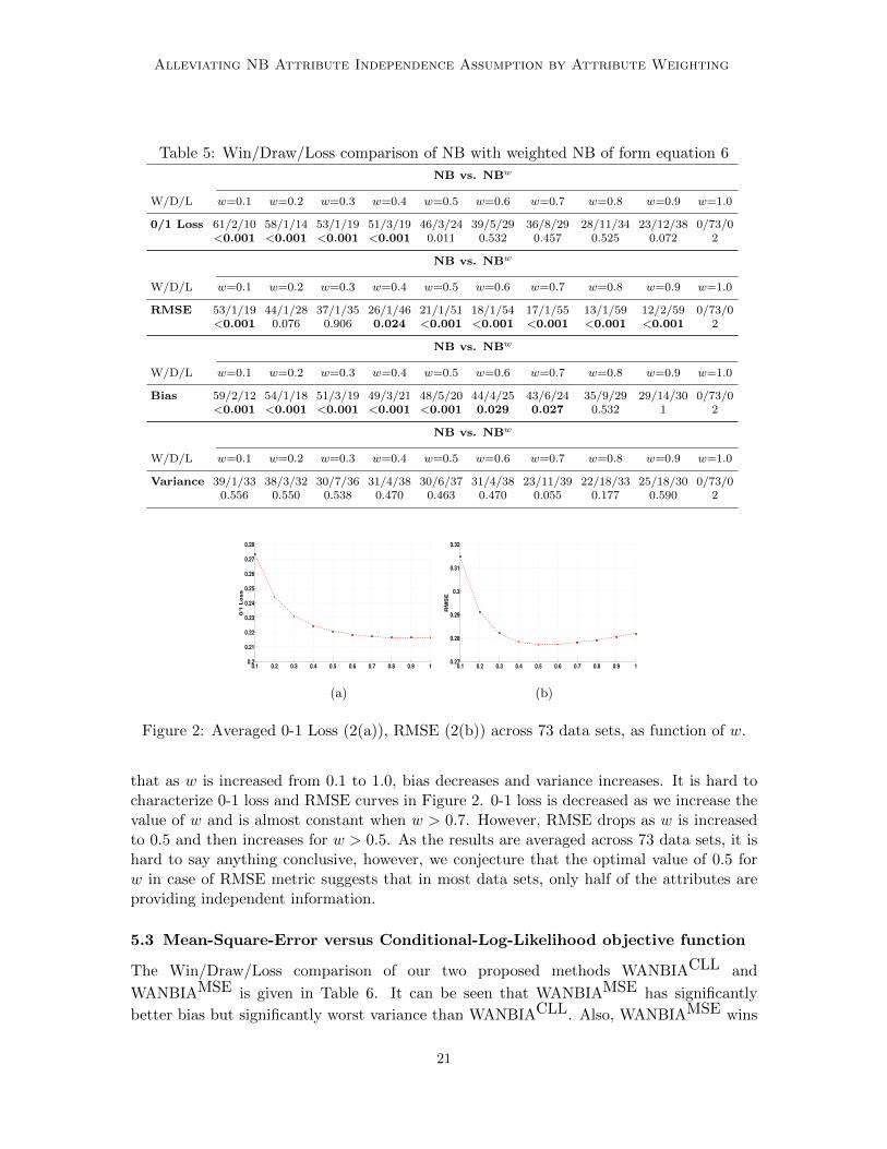
In this section, we will employ the Win/Draw/Loss record (WDL) and simple arithmeticmean to summarize the effects of weights on naive Bayes’ classification performance. Table 5compares the WDL of naive Bayes in equation 3 with weighted naive Bayes in equation 6as the weight w is varied from 0.1 to 1.0. The WDL are presented for 0-1 loss, RMSE, biasand variance. The results reveal that higher value of w e.g., w = 0.9 results in significantlybetter performance in terms of 0-1 loss and RMSE and non-significantly better performancein terms of bias and variance as compared to the lower values.
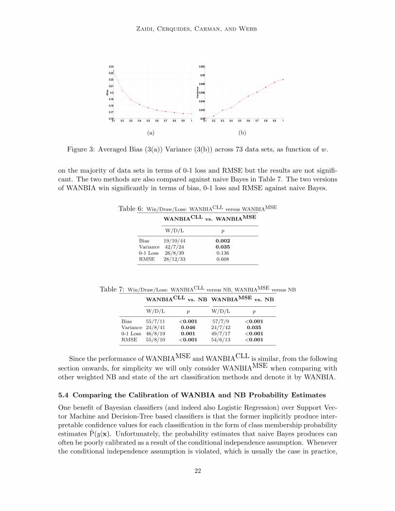
Averaged (arithmetic mean) 0-1 loss, RMSE, bias and variance results across 73 datasets as a function of weight are plotted in Figure 2 and 3. As can be seen from the figures
20
Alleviating NB Attribute Independence Assumption by Attribute Weighting
Table 5: Win/Draw/Loss comparison of NB with weighted NB of form equation 6
NB vs. NBw
W/D/L w=0.1 w=0.2 w=0.3 w=0.4 w=0.5 w=0.6 w=0.7 w=0.8 w=0.9 w=1.0
0/1 Loss 61/2/10 58/1/14 53/1/19 51/3/19 46/3/24 39/5/29 36/8/29 28/11/34 23/12/38 0/73/0<0.001 <0.001 <0.001 <0.001 0.011 0.532 0.457 0.525 0.072 2
NB vs. NBw
W/D/L w=0.1 w=0.2 w=0.3 w=0.4 w=0.5 w=0.6 w=0.7 w=0.8 w=0.9 w=1.0
RMSE 53/1/19 44/1/28 37/1/35 26/1/46 21/1/51 18/1/54 17/1/55 13/1/59 12/2/59 0/73/0<0.001 0.076 0.906 0.024 <0.001 <0.001 <0.001 <0.001 <0.001 2
NB vs. NBw
W/D/L w=0.1 w=0.2 w=0.3 w=0.4 w=0.5 w=0.6 w=0.7 w=0.8 w=0.9 w=1.0
Bias 59/2/12 54/1/18 51/3/19 49/3/21 48/5/20 44/4/25 43/6/24 35/9/29 29/14/30 0/73/0<0.001 <0.001 <0.001 <0.001 <0.001 0.029 0.027 0.532 1 2
NB vs. NBw
W/D/L w=0.1 w=0.2 w=0.3 w=0.4 w=0.5 w=0.6 w=0.7 w=0.8 w=0.9 w=1.0
Variance 39/1/33 38/3/32 30/7/36 31/4/38 30/6/37 31/4/38 23/11/39 22/18/33 25/18/30 0/73/00.556 0.550 0.538 0.470 0.463 0.470 0.055 0.177 0.590 2
0.1 0.2 0.3 0.4 0.5 0.6 0.7 0.8 0.9 10.2
0.21
0.22
0.23
0.24
0.25
0.26
0.27
0.28
0/1
Lo
ss
(a)
0.1 0.2 0.3 0.4 0.5 0.6 0.7 0.8 0.9 10.27
0.28
0.29
0.3
0.31
0.32
RMSE
(b)
Figure 2: Averaged 0-1 Loss (2(a)), RMSE (2(b)) across 73 data sets, as function of w.
that as w is increased from 0.1 to 1.0, bias decreases and variance increases. It is hard tocharacterize 0-1 loss and RMSE curves in Figure 2. 0-1 loss is decreased as we increase thevalue of w and is almost constant when w > 0.7. However, RMSE drops as w is increasedto 0.5 and then increases for w > 0.5. As the results are averaged across 73 data sets, it ishard to say anything conclusive, however, we conjecture that the optimal value of 0.5 forw in case of RMSE metric suggests that in most data sets, only half of the attributes areproviding independent information.
5.3 Mean-Square-Error versus Conditional-Log-Likelihood objective function
The Win/Draw/Loss comparison of our two proposed methods WANBIACLL and
WANBIAMSE is given in Table 6. It can be seen that WANBIAMSE has significantly
better bias but significantly worst variance than WANBIACLL. Also, WANBIAMSE wins
21
Zaidi, Cerquides, Carman, and Webb
0.1 0.2 0.3 0.4 0.5 0.6 0.7 0.8 0.9 10.16
0.17
0.18
0.19
0.2
0.21
0.22
0.23
0.24
Bias
(a)
0.1 0.2 0.3 0.4 0.5 0.6 0.7 0.8 0.9 10.04
0.042
0.044
0.046
0.048
0.05
0.052
Variance
(b)
Figure 3: Averaged Bias (3(a)) Variance (3(b)) across 73 data sets, as function of w.
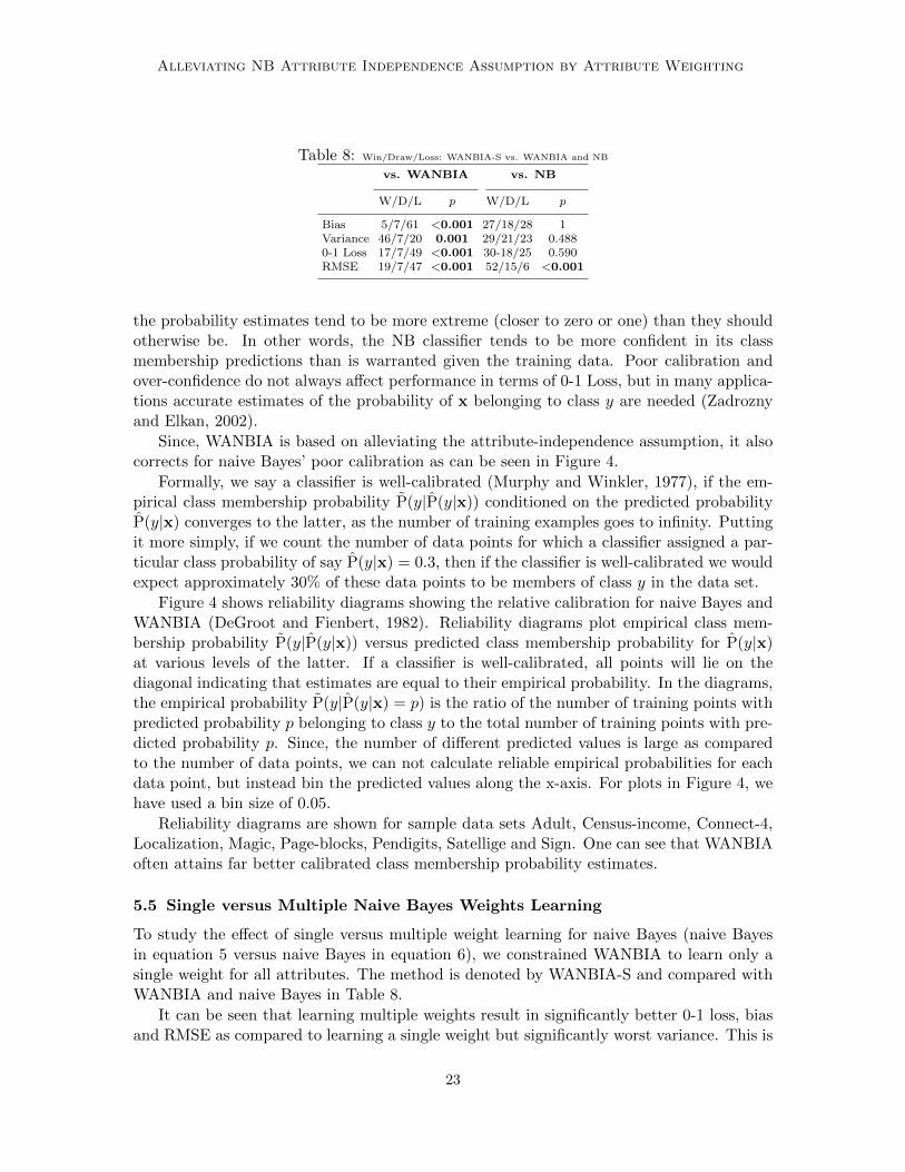
on the majority of data sets in terms of 0-1 loss and RMSE but the results are not signifi-cant. The two methods are also compared against naive Bayes in Table 7. The two versionsof WANBIA win significantly in terms of bias, 0-1 loss and RMSE against naive Bayes.
Table 6: Win/Draw/Loss: WANBIACLL versus WANBIAMSE
WANBIACLL vs. WANBIAMSE
W/D/L p
Bias 19/10/44 0.002Variance 42/7/24 0.0350-1 Loss 26/8/39 0.136RMSE 28/12/33 0.608
Table 7: Win/Draw/Loss: WANBIACLL versus NB, WANBIAMSE versus NB
WANBIACLL vs. NB WANBIAMSE vs. NB
W/D/L p W/D/L p
Bias 55/7/11 <0.001 57/7/9 <0.001Variance 24/8/41 0.046 24/7/42 0.0350-1 Loss 46/8/19 0.001 49/7/17 <0.001RMSE 55/8/10 <0.001 54/6/13 <0.001
Since the performance of WANBIAMSE and WANBIACLL is similar, from the following
section onwards, for simplicity we will only consider WANBIAMSE when comparing withother weighted NB and state of the art classification methods and denote it by WANBIA.
5.4 Comparing the Calibration of WANBIA and NB Probability Estimates
One benefit of Bayesian classifiers (and indeed also Logistic Regression) over Support Vec-tor Machine and Decision-Tree based classifiers is that the former implicitly produce inter-pretable confidence values for each classification in the form of class membership probabilityestimates P(y|x). Unfortunately, the probability estimates that naive Bayes produces canoften be poorly calibrated as a result of the conditional independence assumption. Wheneverthe conditional independence assumption is violated, which is usually the case in practice,
22
Alleviating NB Attribute Independence Assumption by Attribute Weighting
Table 8: Win/Draw/Loss: WANBIA-S vs. WANBIA and NB
vs. WANBIA vs. NB
W/D/L p W/D/L p
Bias 5/7/61 <0.001 27/18/28 1Variance 46/7/20 0.001 29/21/23 0.4880-1 Loss 17/7/49 <0.001 30-18/25 0.590RMSE 19/7/47 <0.001 52/15/6 <0.001
the probability estimates tend to be more extreme (closer to zero or one) than they shouldotherwise be. In other words, the NB classifier tends to be more confident in its classmembership predictions than is warranted given the training data. Poor calibration andover-confidence do not always affect performance in terms of 0-1 Loss, but in many applica-tions accurate estimates of the probability of x belonging to class y are needed (Zadroznyand Elkan, 2002).
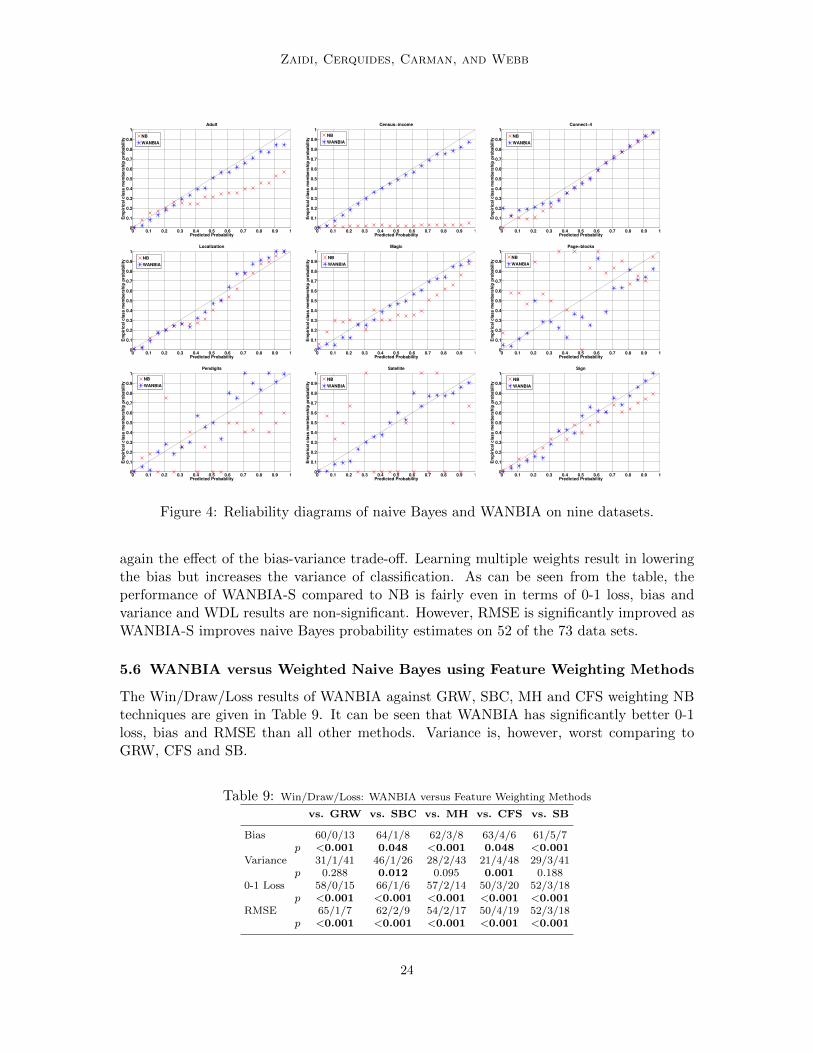
Since, WANBIA is based on alleviating the attribute-independence assumption, it alsocorrects for naive Bayes’ poor calibration as can be seen in Figure 4.
Formally, we say a classifier is well-calibrated (Murphy and Winkler, 1977), if the em-pirical class membership probability P(y|P(y|x)) conditioned on the predicted probabilityP(y|x) converges to the latter, as the number of training examples goes to infinity. Puttingit more simply, if we count the number of data points for which a classifier assigned a par-ticular class probability of say P(y|x) = 0.3, then if the classifier is well-calibrated we wouldexpect approximately 30% of these data points to be members of class y in the data set.
Figure 4 shows reliability diagrams showing the relative calibration for naive Bayes andWANBIA (DeGroot and Fienbert, 1982). Reliability diagrams plot empirical class mem-bership probability P(y|P(y|x)) versus predicted class membership probability for P(y|x)at various levels of the latter. If a classifier is well-calibrated, all points will lie on thediagonal indicating that estimates are equal to their empirical probability. In the diagrams,the empirical probability P(y|P(y|x) = p) is the ratio of the number of training points withpredicted probability p belonging to class y to the total number of training points with pre-dicted probability p. Since, the number of different predicted values is large as comparedto the number of data points, we can not calculate reliable empirical probabilities for eachdata point, but instead bin the predicted values along the x-axis. For plots in Figure 4, wehave used a bin size of 0.05.
Reliability diagrams are shown for sample data sets Adult, Census-income, Connect-4,Localization, Magic, Page-blocks, Pendigits, Satellige and Sign. One can see that WANBIAoften attains far better calibrated class membership probability estimates.
5.5 Single versus Multiple Naive Bayes Weights Learning
To study the effect of single versus multiple weight learning for naive Bayes (naive Bayesin equation 5 versus naive Bayes in equation 6), we constrained WANBIA to learn only asingle weight for all attributes. The method is denoted by WANBIA-S and compared withWANBIA and naive Bayes in Table 8.
It can be seen that learning multiple weights result in significantly better 0-1 loss, biasand RMSE as compared to learning a single weight but significantly worst variance. This is
23
Zaidi, Cerquides, Carman, and Webb
0 0.1 0.2 0.3 0.4 0.5 0.6 0.7 0.8 0.9 10
0.1
0.2
0.3
0.4
0.5
0.6
0.7
0.8
0.9
1
Predicted Probability
Em
pir
ica
l c
las
s m
em
be
rsh
ip p
rob
ab
ilit
yAdult
NB
WANBIA
0 0.1 0.2 0.3 0.4 0.5 0.6 0.7 0.8 0.9 10
0.1
0.2
0.3
0.4
0.5
0.6
0.7
0.8
0.9
1
Predicted Probability
Em
pir
ica
l c
las
s m
em
be
rsh
ip p
rob
ab
ilit
y
Census−income
NB
WANBIA
0 0.1 0.2 0.3 0.4 0.5 0.6 0.7 0.8 0.9 10
0.1
0.2
0.3
0.4
0.5
0.6
0.7
0.8
0.9
1
Predicted Probability
Em
pir
ica
l c
las
s m
em
be
rsh
ip p
rob
ab
ilit
y
Connect−4
NB
WANBIA
0 0.1 0.2 0.3 0.4 0.5 0.6 0.7 0.8 0.9 10
0.1
0.2
0.3
0.4
0.5
0.6
0.7
0.8
0.9
1
Predicted Probability
Em
pir
ica
l c
las
s m
em
be
rsh
ip p
rob
ab
ilit
y
Localization
NB
WANBIA
0 0.1 0.2 0.3 0.4 0.5 0.6 0.7 0.8 0.9 10
0.1
0.2
0.3
0.4
0.5
0.6
0.7
0.8
0.9
1
Predicted Probability
Em
pir
ica
l c
las
s m
em
be
rsh
ip p
rob
ab
ilit
y
Magic
NB
WANBIA
0 0.1 0.2 0.3 0.4 0.5 0.6 0.7 0.8 0.9 10
0.1
0.2
0.3
0.4
0.5
0.6
0.7
0.8
0.9
1
Predicted Probability
Em
pir
ica
l c
las
s m
em
be
rsh
ip p
rob
ab
ilit
y
Page−blocks
NB
WANBIA
0 0.1 0.2 0.3 0.4 0.5 0.6 0.7 0.8 0.9 10
0.1
0.2
0.3
0.4
0.5
0.6
0.7
0.8
0.9
1
Predicted Probability
Em
pir
ica
l c
las
s m
em
be
rsh
ip p
rob
ab
ilit
y
Pendigits
NB
WANBIA
0 0.1 0.2 0.3 0.4 0.5 0.6 0.7 0.8 0.9 10
0.1
0.2
0.3
0.4
0.5
0.6
0.7
0.8
0.9
1
Predicted Probability
Em
pir
ica
l c
las
s m
em
be
rsh
ip p
rob
ab
ilit
y
Satellite
NB
WANBIA
0 0.1 0.2 0.3 0.4 0.5 0.6 0.7 0.8 0.9 10
0.1
0.2
0.3
0.4
0.5
0.6
0.7
0.8
0.9
1
Predicted Probability
Em
pir
ica
l c
las
s m
em
be
rsh
ip p
rob
ab
ilit
y
Sign
NB
WANBIA
Figure 4: Reliability diagrams of naive Bayes and WANBIA on nine datasets.
again the effect of the bias-variance trade-off. Learning multiple weights result in loweringthe bias but increases the variance of classification. As can be seen from the table, theperformance of WANBIA-S compared to NB is fairly even in terms of 0-1 loss, bias andvariance and WDL results are non-significant. However, RMSE is significantly improved asWANBIA-S improves naive Bayes probability estimates on 52 of the 73 data sets.
5.6 WANBIA versus Weighted Naive Bayes using Feature Weighting Methods
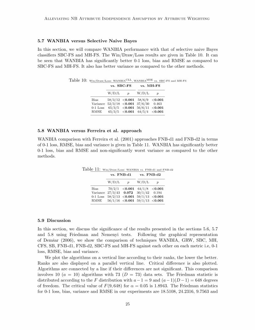
The Win/Draw/Loss results of WANBIA against GRW, SBC, MH and CFS weighting NBtechniques are given in Table 9. It can be seen that WANBIA has significantly better 0-1loss, bias and RMSE than all other methods. Variance is, however, worst comparing toGRW, CFS and SB.
Table 9: Win/Draw/Loss: WANBIA versus Feature Weighting Methods
vs. GRW vs. SBC vs. MH vs. CFS vs. SB
Bias 60/0/13 64/1/8 62/3/8 63/4/6 61/5/7p <0.001 0.048 <0.001 0.048 <0.001
Variance 31/1/41 46/1/26 28/2/43 21/4/48 29/3/41p 0.288 0.012 0.095 0.001 0.188
0-1 Loss 58/0/15 66/1/6 57/2/14 50/3/20 52/3/18p <0.001 <0.001 <0.001 <0.001 <0.001
RMSE 65/1/7 62/2/9 54/2/17 50/4/19 52/3/18p <0.001 <0.001 <0.001 <0.001 <0.001
24
Alleviating NB Attribute Independence Assumption by Attribute Weighting
5.7 WANBIA versus Selective Naive Bayes
In this section, we will compare WANBIA performance with that of selective naive Bayesclassifiers SBC-FS and MH-FS. The Win/Draw/Loss results are given in Table 10. It canbe seen that WANBIA has significantly better 0-1 loss, bias and RMSE as compared toSBC-FS and MH-FS. It also has better variance as compared to the other methods.
Table 10: Win/Draw/Loss: WANBIACLL, WANBIAMSE vs. SBC-FS and MH-FS
vs. SBC-FS vs. MH-FS
W/D/L p W/D/L p
Bias 58/3/12 <0.001 58/6/9 <0.001Variance 52/3/18 <0.001 37/6/30 0.4630-1 Loss 65/3/5 <0.001 56/6/11 <0.001RMSE 65/3/5 <0.001 64/5/4 <0.001
5.8 WANBIA versus Ferreira et al. approach
WANBIA comparison with Ferreira et al. (2001) approaches FNB-d1 and FNB-d2 in termsof 0-1 loss, RMSE, bias and variance is given in Table 11. WANBIA has significantly better0-1 loss, bias and RMSE and non-significantly worst variance as compared to the othermethods.
Table 11: Win/Draw/Loss: WANBIA vs. FNB-d1 and FNB-d2
vs. FNB-d1 vs. FNB-d2
W/D/L p W/D/L p
Bias 70/2/1 <0.001 64/1/8 <0.001Variance 27/3/43 0.072 30/1/42 0.1940-1 Loss 58/2/13 <0.001 59/1/13 <0.001RMSE 56/1/16 <0.001 59/1/13 <0.001
5.9 Discussion
In this section, we discuss the significance of the results presented in the sections 5.6, 5.7and 5.8 using Friedman and Nemenyi tests. Following the graphical representationof Demsar (2006), we show the comparison of techniques WANBIA, GRW, SBC, MH,CFS, SB, FNB-d1, FNB-d2, SBC-FS and MH-FS against each other on each metric i.e, 0-1loss, RMSE, bias and variance.
We plot the algorithms on a vertical line according to their ranks, the lower the better.Ranks are also displayed on a parallel vertical line. Critical difference is also plotted.Algorithms are connected by a line if their differences are not significant. This comparisoninvolves 10 (a = 10) algorithms with 73 (D = 73) data sets. The Friedman statistic isdistributed according to the F distribution with a−1 = 9 and (a−1)(D−1) = 648 degreesof freedom. The critical value of F (9, 648) for α = 0.05 is 1.8943. The Friedman statisticsfor 0-1 loss, bias, variance and RMSE in our experiments are 18.5108, 24.2316, 9.7563 and
25
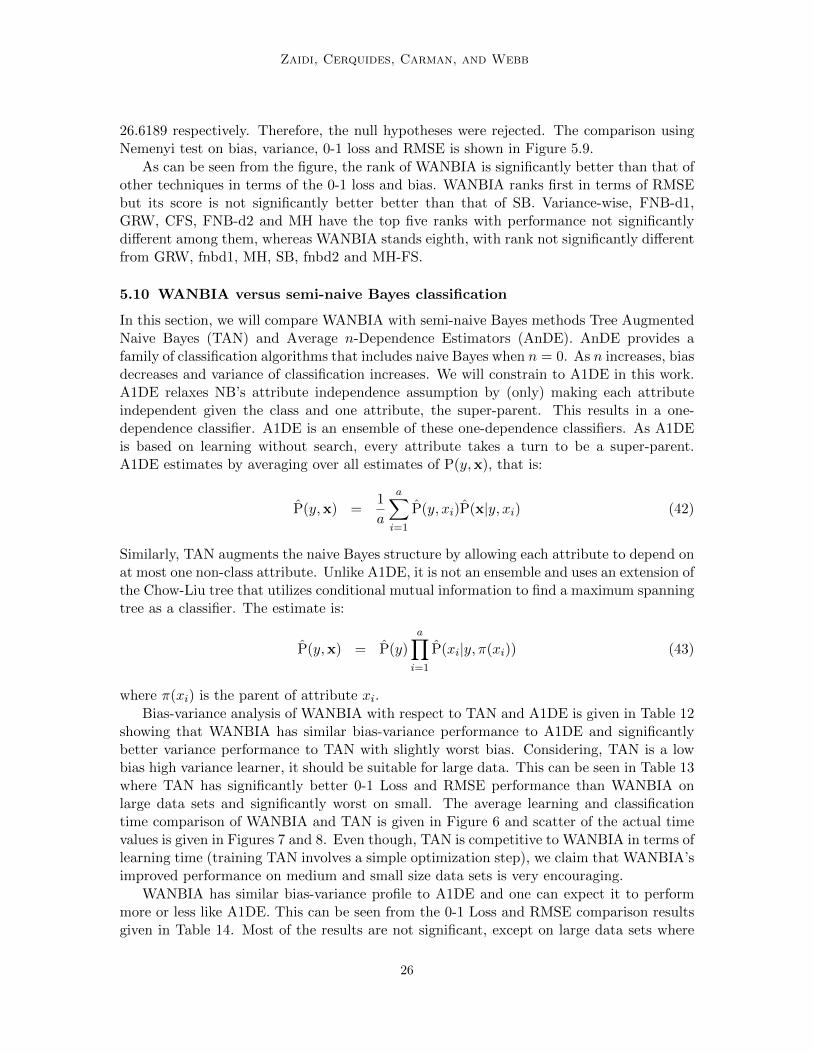
Zaidi, Cerquides, Carman, and Webb
26.6189 respectively. Therefore, the null hypotheses were rejected. The comparison usingNemenyi test on bias, variance, 0-1 loss and RMSE is shown in Figure 5.9.
As can be seen from the figure, the rank of WANBIA is significantly better than that ofother techniques in terms of the 0-1 loss and bias. WANBIA ranks first in terms of RMSEbut its score is not significantly better better than that of SB. Variance-wise, FNB-d1,GRW, CFS, FNB-d2 and MH have the top five ranks with performance not significantlydifferent among them, whereas WANBIA stands eighth, with rank not significantly differentfrom GRW, fnbd1, MH, SB, fnbd2 and MH-FS.
5.10 WANBIA versus semi-naive Bayes classification
In this section, we will compare WANBIA with semi-naive Bayes methods Tree AugmentedNaive Bayes (TAN) and Average n-Dependence Estimators (AnDE). AnDE provides afamily of classification algorithms that includes naive Bayes when n = 0. As n increases, biasdecreases and variance of classification increases. We will constrain to A1DE in this work.A1DE relaxes NB’s attribute independence assumption by (only) making each attributeindependent given the class and one attribute, the super-parent. This results in a one-dependence classifier. A1DE is an ensemble of these one-dependence classifiers. As A1DEis based on learning without search, every attribute takes a turn to be a super-parent.A1DE estimates by averaging over all estimates of P(y,x), that is:
P(y,x) =1
a
a∑i=1
P(y, xi)P(x|y, xi) (42)
Similarly, TAN augments the naive Bayes structure by allowing each attribute to depend onat most one non-class attribute. Unlike A1DE, it is not an ensemble and uses an extension ofthe Chow-Liu tree that utilizes conditional mutual information to find a maximum spanningtree as a classifier. The estimate is:
P(y,x) = P(y)a∏i=1
P(xi|y, π(xi)) (43)
where π(xi) is the parent of attribute xi.
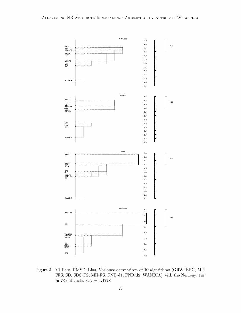
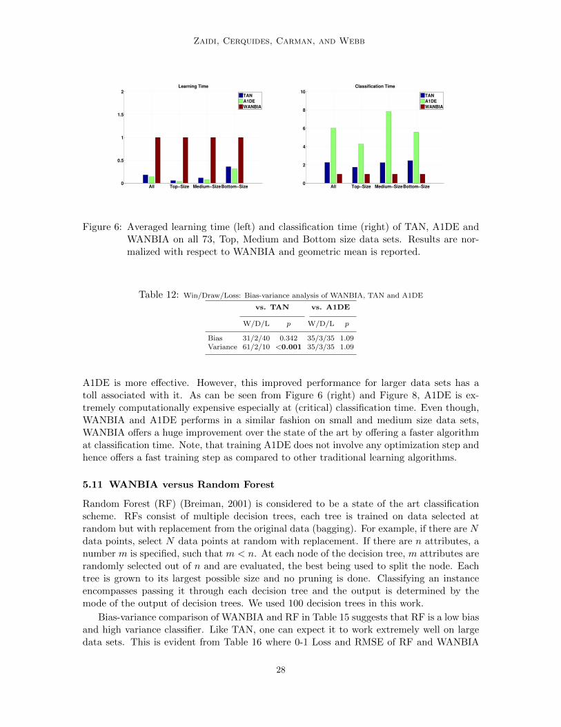
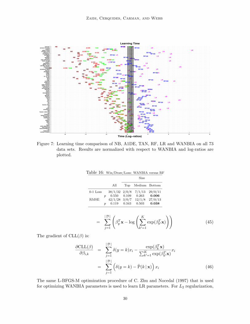
Bias-variance analysis of WANBIA with respect to TAN and A1DE is given in Table 12showing that WANBIA has similar bias-variance performance to A1DE and significantlybetter variance performance to TAN with slightly worst bias. Considering, TAN is a lowbias high variance learner, it should be suitable for large data. This can be seen in Table 13where TAN has significantly better 0-1 Loss and RMSE performance than WANBIA onlarge data sets and significantly worst on small. The average learning and classificationtime comparison of WANBIA and TAN is given in Figure 6 and scatter of the actual timevalues is given in Figures 7 and 8. Even though, TAN is competitive to WANBIA in terms oflearning time (training TAN involves a simple optimization step), we claim that WANBIA’simproved performance on medium and small size data sets is very encouraging.
WANBIA has similar bias-variance profile to A1DE and one can expect it to performmore or less like A1DE. This can be seen from the 0-1 Loss and RMSE comparison resultsgiven in Table 14. Most of the results are not significant, except on large data sets where
26
Alleviating NB Attribute Independence Assumption by Attribute Weighting
0−1 Loss
WANBIA
SBCFSMH
MH−FS
GRWfnbd2
SBC−FS
SBC
fnbd1
2.0
2.5
3.0
3.5
4.0
4.5
5.0
5.5
6.0
6.5
7.0
7.5
8.0
CD
RMSE
WANBIA
SB
CFS
MH
MH−FS
fnbd2SBC
SBC−FS
fnbd1
GRW
2.0
2.5
3.0
3.5
4.0
4.5
5.0
5.5
6.0
6.5
7.0
7.5
8.0
CD
Bias
WANBIA
SBSBC−FSMH−FS
MHCFS
GRW
SBC
fnbd2
fnbd1
2.0
2.5
3.0
3.5
4.0
4.5
5.0
5.5
6.0
6.5
7.0
7.5
8.0
CD
Variance
CFS
GRW
fnbd1MHSB
fnbd2
MH−FS
WANBIA
SBC
SBC−FS
4.0
4.5
5.0
5.5
6.0
6.5
7.0
7.5
8.0
CD
Figure 5: 0-1 Loss, RMSE, Bias, Variance comparison of 10 algorithms (GRW, SBC, MH,CFS, SB, SBC-FS, MH-FS, FNB-d1, FNB-d2, WANBIA) with the Nemenyi teston 73 data sets. CD = 1.4778.
27
Zaidi, Cerquides, Carman, and Webb
All Top−Size Medium−SizeBottom−Size0
0.5
1
1.5
2
Learning Time
TAN
A1DE
WANBIA
All Top−Size Medium−SizeBottom−Size0
2
4
6
8
10
Classification Time
TAN
A1DE
WANBIA
Figure 6: Averaged learning time (left) and classification time (right) of TAN, A1DE andWANBIA on all 73, Top, Medium and Bottom size data sets. Results are nor-malized with respect to WANBIA and geometric mean is reported.
Table 12: Win/Draw/Loss: Bias-variance analysis of WANBIA, TAN and A1DE
vs. TAN vs. A1DE
W/D/L p W/D/L p
Bias 31/2/40 0.342 35/3/35 1.09Variance 61/2/10 <0.001 35/3/35 1.09
A1DE is more effective. However, this improved performance for larger data sets has atoll associated with it. As can be seen from Figure 6 (right) and Figure 8, A1DE is ex-tremely computationally expensive especially at (critical) classification time. Even though,WANBIA and A1DE performs in a similar fashion on small and medium size data sets,WANBIA offers a huge improvement over the state of the art by offering a faster algorithmat classification time. Note, that training A1DE does not involve any optimization step andhence offers a fast training step as compared to other traditional learning algorithms.
5.11 WANBIA versus Random Forest
Random Forest (RF) (Breiman, 2001) is considered to be a state of the art classificationscheme. RFs consist of multiple decision trees, each tree is trained on data selected atrandom but with replacement from the original data (bagging). For example, if there are Ndata points, select N data points at random with replacement. If there are n attributes, anumber m is specified, such that m < n. At each node of the decision tree, m attributes arerandomly selected out of n and are evaluated, the best being used to split the node. Eachtree is grown to its largest possible size and no pruning is done. Classifying an instanceencompasses passing it through each decision tree and the output is determined by themode of the output of decision trees. We used 100 decision trees in this work.
Bias-variance comparison of WANBIA and RF in Table 15 suggests that RF is a low biasand high variance classifier. Like TAN, one can expect it to work extremely well on largedata sets. This is evident from Table 16 where 0-1 Loss and RMSE of RF and WANBIA
28
Alleviating NB Attribute Independence Assumption by Attribute Weighting
Table 13: Win/Draw/Loss: WANBIA versus TAN
Size
All Top Medium Bottom
0-1 Loss 48/2/23 2/0/10 14/1/6 32/1/7p 0.004 0.038 0.115 <0.001
RMSE 46/1/26 2/0/10 14/1/6 30/0/10p 0.024 0.038 0.115 0.002
Table 14: Win/Draw/Loss: WANBIA versus A1DE
Size
All Top Medium Bottom
0-1 Loss 31/4/38 2/1/9 10/1/10 19/2/19p 0.470 0.065 1.176 1.128
RMSE 30/3/40 2/0/10 9/1/11 19/2/19p 0.282 0.038 0.823 1.128
is compared. Note, we were unable to compute results for RF on our two largest data setsPoker-hand and Covertype (Table 4). Even with 32 GB of RAM, Weka exhausted heapmemory during cross-validation experiments on RF for these data sets. However, due toits low bias one would expect RF to beat WANBIA on these two data sets, resulting inW/D/L of 2/0/10 and 3/0/9 on largest datasets for 0-1 Loss and RMSE with a significanceof 0.038 and 0.146.
Table 15: Win/Draw/Loss: Bias-variance analysis of WANBIA and RF
vs. RF
W/D/L p
Bias 21/2/48 0.001Variance 53/3/16 <0.001
On smaller datasets WANBIA has a better 0-1 Loss performance and significantly betterRMSE than RF. This is packaged with WANBIA’s far superior learning and classificationtimings over RF as can be seen from Figures 7, 8 and 9,. This makes WANBIA an excellentalternative to RF especially for small data.
5.12 WANBIA versus Logistic Regression
In this section, we compare the performance of WANBIA with state of the art discriminativeclassifier Logistic Regression (LR). We implemented LR as described in Roos et al. (2005).The following objective function is optimized:
CLL(β) =
|D|∑j=1
log P(y|x) (44)
29
Zaidi, Cerquides, Carman, and Webb
−6 −4 −2 0 2 4 6 8
contact−lenseshaberman
taeechocardiogram
new−thyroidpost−operative
bupairis
winelabor
glass3zoo
clevelandhungarian
balance−scalehepatitis
ledhouse−votes−84
pidvolcanoes
yeastlynttt
horse−coliccrxcar
cmcptn
bcwvowel
vehiclegerman
autosionosphere
chesssonar
abalonedermatology
promoterslung−cancerpage−blocks
annealsegmentnursery
signsick
hypokr−vs−kp
mushaudiomagic
pendigitssyncon
waveform−5000thyroid
phonemecylinder−bands
splice−c4.5spambase
musk1letter−recog
wall−followingshuttle
satelliteadult
optdigitslocalizationconnect−4
covtype−modpoker−hand
musk2census−income
pioneer
Time (Log−ratios)
Learning Time
A1DEA1DE
A1DEA1DE
A1DEA1DE
A1DEA1DE
A1DEA1DE
A1DEA1DE
A1DEA1DE
A1DEA1DE
A1DEA1DE
A1DEA1DE
A1DEA1DE
A1DEA1DE
A1DEA1DE
A1DEA1DE
A1DEA1DE
A1DEA1DE
A1DEA1DE
A1DEA1DE
A1DEA1DE
A1DEA1DE
A1DEA1DE
A1DEA1DE
A1DEA1DE
A1DEA1DE
A1DEA1DE
A1DEA1DE
A1DEA1DE
A1DEA1DE
A1DEA1DE
A1DEA1DE
A1DEA1DE
A1DEA1DE
A1DEA1DE
A1DEA1DE
A1DEA1DE
A1DEA1DE
A1DE
LRLR
LRLR
LRLR
LRLR
LRLR
LRLR
LRLR
LRLR
LRLRLR
LRLR
LRLR
LRLR
LRLR
LRLR
LRLR
LRLR
LRLR
LRLR
LRLR
LRLR
LRLR
LRLR
LRLR
LRLR
LRLR
LRLR
LRLR
LRLR
LRLR
LRLR
LRLR
LRLR
LRLR
LRLR
LRLR
LRLR
NBNB
NBNB
NBNB
NBNB
NBNB
NBNBNB
NBNB
NBNB
NBNB
NBNB
NBNB
NBNB
NBNB
NBNB
NBNB
NBNBNB
NBNB
NBNB
NBNB
NBNB
NBNB
NBNB
NBNB
NBNB
NBNB
NBNB
NBNB
NBNBNB
NBNB
NBNB
NBNB
NBNBNB
NBNB
NBNB
NB
WANBIAWANBIAWANBIAWANBIAWANBIAWANBIAWANBIAWANBIAWANBIAWANBIAWANBIAWANBIAWANBIAWANBIAWANBIAWANBIAWANBIAWANBIAWANBIAWANBIAWANBIAWANBIAWANBIAWANBIAWANBIAWANBIAWANBIAWANBIAWANBIAWANBIAWANBIAWANBIAWANBIAWANBIAWANBIAWANBIAWANBIAWANBIAWANBIAWANBIAWANBIAWANBIAWANBIAWANBIAWANBIAWANBIAWANBIAWANBIAWANBIAWANBIAWANBIAWANBIAWANBIAWANBIAWANBIAWANBIAWANBIAWANBIAWANBIAWANBIAWANBIAWANBIAWANBIAWANBIAWANBIAWANBIAWANBIAWANBIAWANBIAWANBIAWANBIAWANBIAWANBIA
RF100RF100
RF100RF100
RF100RF100
RF100RF100
RF100RF100
RF100RF100
RF100RF100
RF100RF100
RF100RF100
RF100RF100
RF100RF100
RF100RF100
RF100RF100
RF100RF100
RF100RF100
RF100RF100
RF100RF100
RF100RF100
RF100RF100
RF100RF100
RF100RF100
RF100RF100
RF100RF100
RF100RF100
RF100RF100
RF100RF100
RF100RF100
RF100RF100
RF100RF100
RF100RF100
RF100RF100
RF100RF100
RF100RF100
RF100RF100
RF100RF100
RF100
TANTAN
TANTAN
TANTAN
TANTAN
TANTAN
TANTAN
TANTAN
TANTAN
TANTAN
TANTAN
TANTAN
TANTAN
TANTAN
TANTAN
TANTAN
TANTAN
TANTAN
TANTAN
TANTAN
TANTAN
TANTAN
TANTAN
TANTAN
TANTANTAN
TANTAN
TANTAN
TANTAN
TANTAN
TANTAN
TANTAN
TANTAN
TANTAN
TANTAN
TANTAN
TANTAN
TANTAN
Figure 7: Learning time comparison of NB, A1DE, TAN, RF, LR and WANBIA on all 73data sets. Results are normalized with respect to WANBIA and log-ratios areplotted.
Table 16: Win/Draw/Loss: WANBIA versus RF
Size
All Top Medium Bottom
0-1 Loss 38/1/32 2/0/8 7/1/13 29/0/11p 0.550 0.109 0.263 0.006
RMSE 42/1/28 3/0/7 12/1/8 27/0/13p 0.119 0.343 0.503 0.038
=
| D |∑j=1
(βTy x− log
(K∑k′=1
exp(βTk′x)
))(45)
The gradient of CLL(β) is:
∂CLL(β)
∂βi,k=
| D |∑j=1
δ(y = k)xi −exp(βTk x)∑Kk′=1 exp(βTk′x)
xi
=
| D |∑j=1
(δ(y = k)− P(k |x)
)xi (46)
The same L-BFGS-M optimization procedure of C. Zhu and Nocedal (1997) that is usedfor optimizing WANBIA parameters is used to learn LR parameters. For L2 regularization,
30
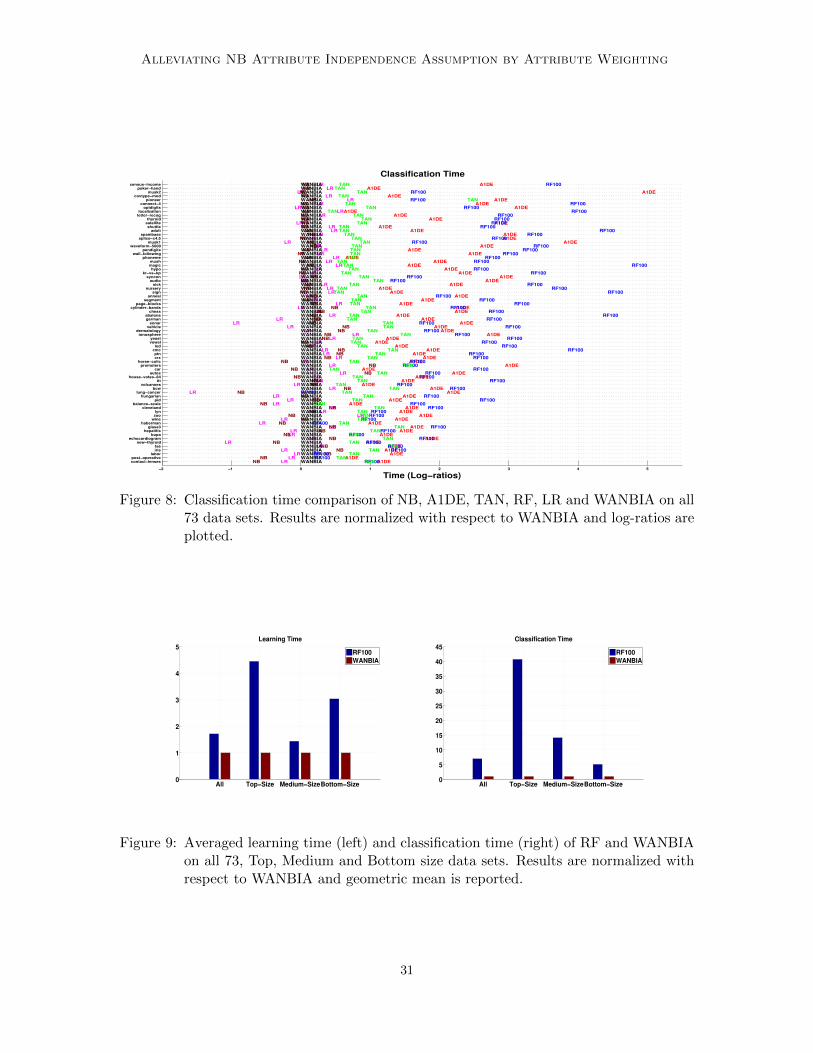
Alleviating NB Attribute Independence Assumption by Attribute Weighting
−2 −1 0 1 2 3 4 5
contact−lensespost−operative
laboriristae
new−thyroidechocardiogram
bupahepatitis
glass3haberman
winezoolyn
clevelandbalance−scale
pidhungarian
lung−cancerbcw
volcanoesttt
house−votes−84autos
carpromoters
horse−coliccrxptn
cmcled
vowelyeast
ionospheredermatology
vehiclesonar
germanabalone
chesscylinder−bands
page−blockssegment
annealsign
nurserysick
audiosyncon
kr−vs−kphypo
magicmush
phonemewall−following
pendigitswaveform−5000
musk1splice−c4.5spambase
adultshuttle
satellitethyroid
letter−recoglocalization
optdigitsconnect−4
pioneercovtype−mod
musk2poker−hand
census−income
Time (Log−ratios)
Classification Time
A1DEA1DE
A1DEA1DE
A1DEA1DE
A1DEA1DE
A1DEA1DE
A1DEA1DE
A1DEA1DE
A1DEA1DE
A1DEA1DE
A1DEA1DE
A1DEA1DE
A1DEA1DE
A1DEA1DE
A1DEA1DE
A1DEA1DE
A1DEA1DE
A1DEA1DE
A1DEA1DE
A1DEA1DE
A1DEA1DEA1DE
A1DEA1DE
A1DEA1DE
A1DEA1DE
A1DEA1DE
A1DEA1DE
A1DEA1DE
A1DEA1DE
A1DEA1DE
A1DEA1DEA1DE
A1DEA1DE
A1DEA1DE
A1DEA1DE
A1DEA1DE
A1DEA1DE
A1DEA1DE
A1DE
LRLR
LRLR
LRLR
LRLRLR
LRLR
LRLR
LRLR
LRLR
LRLR
LRLR
LRLR
LRLR
LRLR
LRLRLR
LRLR
LRLR
LRLR
LRLR
LRLR
LRLR
LRLR
LRLR
LRLR
LRLR
LRLR
LRLR
LRLR
LRLR
LRLR
LRLR
LRLR
LRLR
LRLR
LRLR
LRLR
LR
NBNB
NBNB
NBNB
NBNB
NBNB
NBNB
NBNB
NBNB
NBNB
NBNB
NBNB
NBNB
NBNB
NBNB
NBNB
NBNB
NBNB
NBNB
NBNB
NBNB
NBNB
NBNB
NBNBNB
NBNB
NBNB
NBNB
NBNB
NBNB
NBNB
NBNB
NBNBNBNBNBNB
NBNB
NBNB
NBNB
WANBIAWANBIAWANBIAWANBIAWANBIAWANBIAWANBIAWANBIAWANBIAWANBIAWANBIAWANBIAWANBIAWANBIAWANBIAWANBIAWANBIAWANBIAWANBIAWANBIAWANBIAWANBIAWANBIAWANBIAWANBIAWANBIAWANBIAWANBIAWANBIAWANBIAWANBIAWANBIAWANBIAWANBIAWANBIAWANBIAWANBIAWANBIAWANBIAWANBIAWANBIAWANBIAWANBIAWANBIAWANBIAWANBIAWANBIAWANBIAWANBIAWANBIAWANBIAWANBIAWANBIAWANBIAWANBIAWANBIAWANBIAWANBIAWANBIAWANBIAWANBIAWANBIAWANBIAWANBIAWANBIAWANBIAWANBIAWANBIAWANBIAWANBIAWANBIAWANBIAWANBIA
RF100RF100RF100
RF100RF100
RF100RF100
RF100RF100
RF100RF100
RF100RF100RF100
RF100RF100
RF100RF100
RF100RF100
RF100RF100
RF100RF100
RF100RF100
RF100RF100
RF100RF100
RF100RF100
RF100RF100
RF100RF100
RF100RF100
RF100RF100
RF100RF100
RF100RF100
RF100RF100
RF100RF100
RF100RF100
RF100RF100
RF100RF100
RF100RF100
RF100RF100
RF100RF100
RF100RF100
RF100RF100
RF100RF100
RF100RF100
RF100
RF100
RF100
TANTAN
TANTAN
TANTAN
TANTAN
TANTAN
TANTANTAN
TANTAN
TANTAN
TANTAN
TANTAN
TANTAN
TANTAN
TANTAN
TANTAN
TANTAN
TANTAN
TANTAN
TANTAN
TANTAN
TANTAN
TANTAN
TANTAN
TANTAN
TANTAN
TANTAN
TANTAN
TANTANTANTAN
TANTAN
TANTANTAN
TANTAN
TANTAN
TANTAN
TANTAN
TANTAN
TAN
Figure 8: Classification time comparison of NB, A1DE, TAN, RF, LR and WANBIA on all73 data sets. Results are normalized with respect to WANBIA and log-ratios areplotted.
All Top−Size Medium−SizeBottom−Size0
1
2
3
4
5
Learning Time
RF100
WANBIA
All Top−Size Medium−SizeBottom−Size0
5
10
15
20
25
30
35
40
45
Classification Time
RF100
WANBIA
Figure 9: Averaged learning time (left) and classification time (right) of RF and WANBIAon all 73, Top, Medium and Bottom size data sets. Results are normalized withrespect to WANBIA and geometric mean is reported.
31
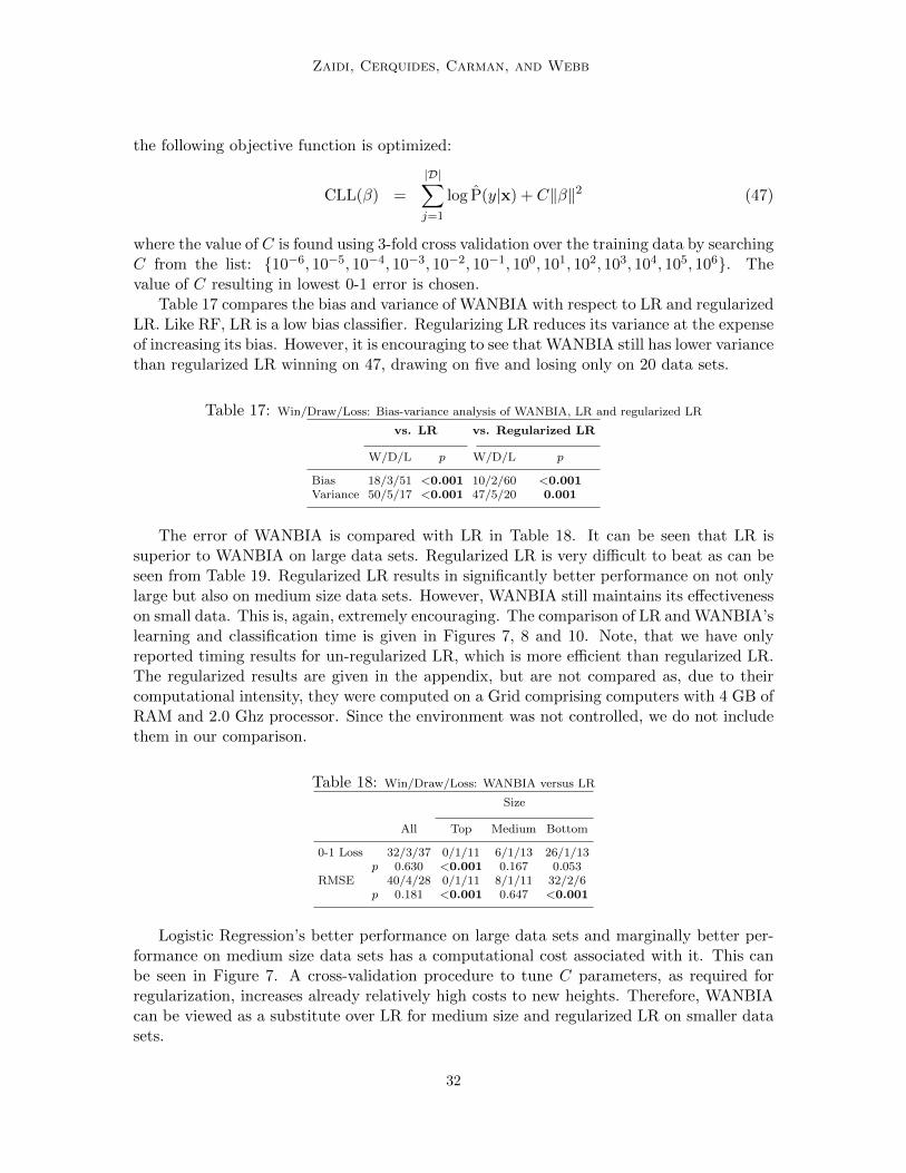
Zaidi, Cerquides, Carman, and Webb
the following objective function is optimized:
CLL(β) =
|D|∑j=1
log P(y|x) + C‖β‖2 (47)
where the value of C is found using 3-fold cross validation over the training data by searchingC from the list: {10−6, 10−5, 10−4, 10−3, 10−2, 10−1, 100, 101, 102, 103, 104, 105, 106}. Thevalue of C resulting in lowest 0-1 error is chosen.
Table 17 compares the bias and variance of WANBIA with respect to LR and regularizedLR. Like RF, LR is a low bias classifier. Regularizing LR reduces its variance at the expenseof increasing its bias. However, it is encouraging to see that WANBIA still has lower variancethan regularized LR winning on 47, drawing on five and losing only on 20 data sets.
Table 17: Win/Draw/Loss: Bias-variance analysis of WANBIA, LR and regularized LR
vs. LR vs. Regularized LR
W/D/L p W/D/L p
Bias 18/3/51 <0.001 10/2/60 <0.001Variance 50/5/17 <0.001 47/5/20 0.001
The error of WANBIA is compared with LR in Table 18. It can be seen that LR issuperior to WANBIA on large data sets. Regularized LR is very difficult to beat as can beseen from Table 19. Regularized LR results in significantly better performance on not onlylarge but also on medium size data sets. However, WANBIA still maintains its effectivenesson small data. This is, again, extremely encouraging. The comparison of LR and WANBIA’slearning and classification time is given in Figures 7, 8 and 10. Note, that we have onlyreported timing results for un-regularized LR, which is more efficient than regularized LR.The regularized results are given in the appendix, but are not compared as, due to theircomputational intensity, they were computed on a Grid comprising computers with 4 GB ofRAM and 2.0 Ghz processor. Since the environment was not controlled, we do not includethem in our comparison.
Table 18: Win/Draw/Loss: WANBIA versus LR
Size
All Top Medium Bottom
0-1 Loss 32/3/37 0/1/11 6/1/13 26/1/13p 0.630 <0.001 0.167 0.053
RMSE 40/4/28 0/1/11 8/1/11 32/2/6p 0.181 <0.001 0.647 <0.001
Logistic Regression’s better performance on large data sets and marginally better per-formance on medium size data sets has a computational cost associated with it. This canbe seen in Figure 7. A cross-validation procedure to tune C parameters, as required forregularization, increases already relatively high costs to new heights. Therefore, WANBIAcan be viewed as a substitute over LR for medium size and regularized LR on smaller datasets.
32
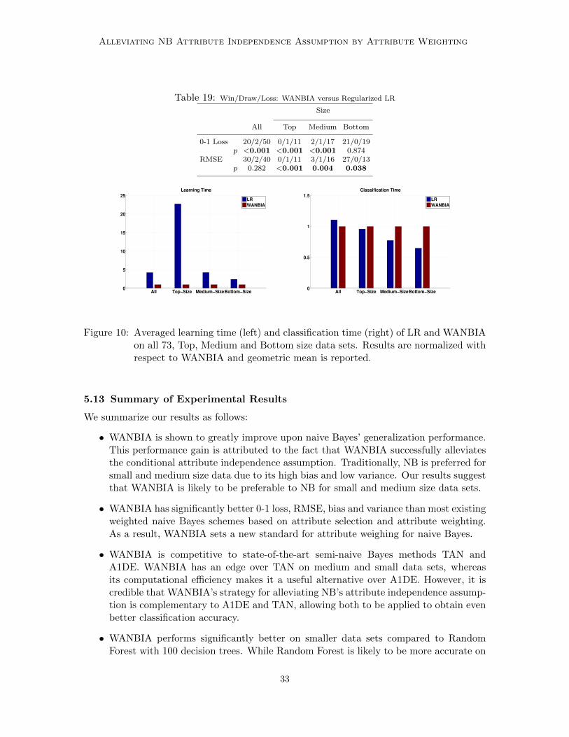
Alleviating NB Attribute Independence Assumption by Attribute Weighting
Table 19: Win/Draw/Loss: WANBIA versus Regularized LR
Size
All Top Medium Bottom
0-1 Loss 20/2/50 0/1/11 2/1/17 21/0/19p <0.001 <0.001 <0.001 0.874
RMSE 30/2/40 0/1/11 3/1/16 27/0/13p 0.282 <0.001 0.004 0.038
All Top−Size Medium−SizeBottom−Size0
5
10
15
20
25
Learning Time
LR
WANBIA
All Top−Size Medium−SizeBottom−Size0
0.5
1
1.5
Classification Time
LR
WANBIA
Figure 10: Averaged learning time (left) and classification time (right) of LR and WANBIAon all 73, Top, Medium and Bottom size data sets. Results are normalized withrespect to WANBIA and geometric mean is reported.
5.13 Summary of Experimental Results
We summarize our results as follows:
• WANBIA is shown to greatly improve upon naive Bayes’ generalization performance.This performance gain is attributed to the fact that WANBIA successfully alleviatesthe conditional attribute independence assumption. Traditionally, NB is preferred forsmall and medium size data due to its high bias and low variance. Our results suggestthat WANBIA is likely to be preferable to NB for small and medium size data sets.
• WANBIA has significantly better 0-1 loss, RMSE, bias and variance than most existingweighted naive Bayes schemes based on attribute selection and attribute weighting.As a result, WANBIA sets a new standard for attribute weighing for naive Bayes.
• WANBIA is competitive to state-of-the-art semi-naive Bayes methods TAN andA1DE. WANBIA has an edge over TAN on medium and small data sets, whereasits computational efficiency makes it a useful alternative over A1DE. However, it iscredible that WANBIA’s strategy for alleviating NB’s attribute independence assump-tion is complementary to A1DE and TAN, allowing both to be applied to obtain evenbetter classification accuracy.
• WANBIA performs significantly better on smaller data sets compared to RandomForest with 100 decision trees. While Random Forest is likely to be more accurate on
33
Zaidi, Cerquides, Carman, and Webb
larger data sets, WANBIA provides a computationally efficient alternative that maybe attractive when computational burden is an issue.
• WANBIA is more accurate than both regularized and unregularized Logistic Regres-sion on smaller data. Also, for multi-class and multi-valued data, WANBIA is basedon optimizing far fewer parameters and, therefore, is computationally more efficientthan LR.
6. Conclusions and Further Research
In this work we have introduced weighting schemes to incorporate weights in naive Bayes.Our work has been primarily motivated by the observation that naive Bayes conditionalattribute independence assumption is often violated and, therefore, it is useful to alleviateit. We build an argument that in current research, weighting in naive Bayes has beenviewed as a way of enhancing the impact of attributes that are highly correlated with theclass. We argue that weighting provides a natural framework for alleviating the attribute
independence assumption. Our two proposed naive Bayes weighting methods WANBIACLL
and WANBIAMSE fix naive Bayes’ parameters to be the MAP estimates and learn weightsby maximizing conditional log-likelihood and minimizing Mean Square Error respectively.This scheme results in the need to optimize significantly fewer parameters than LR.
Conditional log likelihood and mean square error are not the only objective functionsthat can be optimized to learn weights for WANBIA. One can use, for instance, HingeLoss (generally used with SVM) and exponential loss (boosting). Another alternative isusing a different form of mean square error that is 1
2
∑x(j) ∈ |D | (1 − P(y|x))2 instead of
12
∑x(j)∈ |D |
∑y(P(y|x)−P(y|x))2. A comparison of WANBIA trained using these objective
functions has been left to future work.
In interpreting the results presented in this work, it is important to keep in mind thatattribute weighting and semi-naive Bayesian relaxation of the attribute independence as-sumption are mutually compatible. It remains a direction for future research to exploretechniques for attribute weighting in the context of semi-naive Bayes classifiers.
We have constrained ourselves in this work to weighting of the form of equation 5. Itwill be interesting to optimize weights as in equation 4, that is, optimizing a weight for eachattribute’s value. A next step will be to learn a weight for each attribute value per classand a weight for the prior probabilities. Such a variant of WANBIA would have the samenumber of parameters to optimize as Logistic Regression. For example, for i-th attributeand y-th class, weight term constitutes βi,y for LR and wi log θxi|y for WANBIA.
In conclusion, with modest computation, WANBIA substantially decreases the biasof naive Bayes without unduly increasing its variance. The resulting classifier is highlycompetitive with the state of the art when learning from small and medium size datasets.
Acknowledgment
This research has been supported by the Australian Research Council under grantDP110101427 and Asian Office of Aerospace Research and Development, Air Force Of-fice of Scientific Research under contract FA23861214030. The authors would like to thank
34
Alleviating NB Attribute Independence Assumption by Attribute Weighting
Mark Hall for providing the code for CFS and MH. The authors would also like to thankanonymous reviewers for their insightful comments that helped improving the paper tremen-dously.
Appendix A. Code and Detailed Results
The code of the methods proposed in this work can be obtained from the website, http://sourceforge.net/projects/rawnaivebayes/. This appendix presents the detailed resultsfor Error (Table 20), RMSE (Table 21), Bias (Table 22), Variance (Table 23), Train time(Table 24) and Test time (Table 25).
References
R Bellman. Dynamic Programming. Princeton University Press, 1957.
B Bjerregaard, J Holst-Christensen S Brynitz, J Lund-Kristensen E Kalaja, J Hilden, F.TdeDombal, and J.C Horrocks. Computer-aided diagnosis of acute abdomen: a systemfrom leeds used on copenhagen patients. In In Decision Making and Medical Care: CanInformation Science Help. North-Holland Publishing Company, 1976.
Damien Brain and Geoffrey I. Webb. The need for low bias algorithms in classificationlearning from small data sets. In Proceedings of the Sixth European Conference on Prin-ciples and Practice of Knowledge Discovery in Databases (PKDD) 2002, pages 62–73,Berlin, 2002. Springer-Verlag.
L Breiman. Random forests. Machine Learning, 45:5–32, 2001.
R. H. Byrd C. Zhu and J. Nocedal. L-bfgs-b: Algorithm 778: L-bfgs-b, fortran routinesfor large scale bound constrained optimization. ACM Transactions on MathematicalSoftware, 23(4):550–560, 1997.
Alexandra Carvalho, Teemu Roos, Arlindo Oliveira, and Petri Myllymaki. Discriminativelearning of Bayesian networks via factorized conditional log-likelihood. Journal of Ma-chine Learning Research, 2011.
J. Cerquides and R.L. De Mantaras. Tan classifiers based on decomposable distributions.Machine Learning, 59(3):323–354, 2005.
Jesus Cerquides and Ramon Lopez De Mantaras. Robust Bayesian linear classifier ensem-bles. In Proceedings of the Sixteenth European Conference on Machine Learning, pages70–81, 2005.
Bojan Cestnik, Igor Kononenko, and Ivan Bratko. Assistant 86: A knowledge-elicitationtool for sophisticated users. In Proceedings of the Second European Working Session onLearning, pages 31–45. Wulmslow, UK: Sigma Press, 1987.
MH DeGroot and SE Fienbert. The comparison and evaluation of forecasters. Statistician,32(1):12–22, 1982.
35
Zaidi, Cerquides, Carman, and Webb
Janez Demsar. Statistical comparisons of classifiers over multiple data sets. Journal ofMachine Learning Research, 7:1–30, 2006.
Pedro Domingos and Michael J. Pazzani. Beyond independence: Conditions for the opti-mality of the simple Bayesian classifier. In Proceedings of the Thirteenth InternationalConference on Machine Learning, pages 105–112. Morgan Kaufmann, 1996.
R. Duda, P. Hart, and D. Stork. Pattern Classification. John Wiley and Sons, 2006.
Usama M. Fayyad and Keki B. Irani. On the handling of continuous-valued attributes indecision tree generation. Machine Learning, 8(1):87–102, 1992.
J. T. A. S. Ferreira, D. G. T. Denison, and D. J. Hand. Weighted naive Bayes modellingfor data mining, 2001.
A Frank and A Asuncion. UCI machine learning repository, 2010. URL http://archive.
ics.uci.edu/ml.
J Friedman. Flexible metric nearest neighbor classification. Technical report, Departmentof Statistics, Stanford University, 1994.
Milton Friedman. The use of ranks to avoid the assumption of normality implicit in theanalysis of variance. the American Statistical Association, 32(200):675–701, 1937.
Milton Friedman. A comparison of alternative tests of significance for the problem of mrankings. the American Statistical Association, 11(1):86–92, 1940.
Nir Friedman and Moises Goldszmidt. Building classifiers using Bayesian networks. InAAAI-96, pages 1277–1284, 1996.
Nir Friedman, Dan Geiger, and Moises Goldszmidt. Bayesian network classifiers. MachineLearning, 29(2):131–163, 1997.
Russell Greiner, Wei Zhou, Xiaoyuan Su, and Bin Shen. Structural extensions to logisticregression: Discriminative parameter learning of belief net classifiers. Journal of MachineLearning Research, 2004.
Daniel Grossman and Pedro Domingos. Learning Bayesian network classifiers by maximizingcondititional likelihood. In International Conference on Machine Learning, 2004.
I. Guyon, S. Gunn, M. Nikravesh, and L. Zadeh. Feature Extraction, Foundation andApplications. Springer, 2004.
Mark Hall. A decision tree-based attribute weighting filter for naive Bayes. Knowledge-Based Systems, 20:120–126, March 2007.
Mark A. Hall. Correlation-based feature selection for discrete and numeric class machinelearning. In Proceedings of the Seventeenth International Conference on Machine Learn-ing, pages 359–366. Morgan Kaufmann, 2000.
36
Alleviating NB Attribute Independence Assumption by Attribute Weighting
D.J. Hand and K. Yu. Idiot’s Bayes - not so stupid after all? International StatisticalReview, 69(3):385–398, 2001.
J Hilden and B Bjerregaard. Computer-aided diagnosis and the atypical case. In In DecisionMaking and Medical Care: Can Information Science Help, pages 365–378. North-HollandPublishing Company, 1976.
Ron Kohavi and David Wolpert. Bias plus variance decomposition for zero-one loss func-tions. In Proceedings of the Thirteenth International Conference on Machine Learning,pages 275–283. San Francisco: Morgan Kaufmann, 1996.
Igor Kononenko. Comparison of inductive and naive Bayesian learning approaches to au-tomatic knowledge acquisition. 1990.
Pat Langley and Stephanie Sage. Induction of selective Bayesian classifiers. In Proceedingsof the Tenth Conference on Uncertainty in Artificial Intelligence, pages 399–406. MorganKaufmann, 1994.
Pat Langley, Wayne Iba, and Kevin Thompson. An analysis of Bayesian classifiers. InProceedings of the Tenth National Conference on Artificial Intelligence, pages 223–228.AAAI Press and MIT Press, 1992.
David D. Lewis. Naive Bayes at forty: The independence assumption in information re-trieval. In ECML-98: Proceedings of the Tenth European Conference on Machine Learn-ing, pages 4–15, Berlin, April 1998. Springer.
A Murphy and R Winkler. Reliability of subjective probability forcasts of precipitation andtemperature. Applied Statistics, 26(1):41–47, 1977.
Franz Pernkopf and Jeff A. Bilmes. Efficient heuristics for discriminative structure learningof Bayesian network classifiers. Journal of Machine Learning Research, 2010.
C.A Ratanamahatana and D. Gunopulos. Feature selection for the naive Bayesian classifierusing decision trees. pages 475–487, 2003.
Teemu Roos, Hannes Wettig, Peter Grunwald, Petri Myllymaki, and Henry Tirri. Ondiscriminative Bayesian network classifiers and logistic regression. Machine Learning, 59(3):267–296, 2005.
Geoffrey I. Webb. Multiboosting: A technique for combining boosting and wagging. Ma-chine Learning, 40(2):159–196, 2000.
Geoffrey I. Webb, Janice Boughton, and Zhihai Wang. Not so naive Bayes: Averagedone-dependence estimators. Machine Learning, 58(1):5–24, 2005.
Geoffrey I. Webb, Janice Boughton, Fei Zheng, Kai Ming Ting, and Houssam Salem. Learn-ing by extrapolation from marginal to full-multivariate probability distributions: decreas-ingly naive Bayesian classification. Machine Learning, pages 1–40, 2011. ISSN 0885-6125.URL http://dx.doi.org/10.1007/s10994-011-5263-6. 10.1007/s10994-011-5263-6.
37
Zaidi, Cerquides, Carman, and Webb
Jia Wu and Zhihua Cai. Attribute weighting via differential evolution algorithm for attributeweighted naive Bayes (wnb). 7(5):1672–1679, 2011.
B Zadrozny and C Elkan. Transforming classifier scores into accurate multiclass probabilityestimates. In ACM SIGKDD, International Conference on Knowledge Discovery andData Mining, 2002.
H. Zhang and Shengli Sheng. Learning weighted naive Bayes with accurate ranking. InProceedings of the Fourth IEEE International Conference on Data Mining (ICDM -04),pages 567–570, 2004.
Fei Zheng, Geoffrey I. Webb, Pramudi Suraweera, and L Zhu. Subsumption resolution: Anefficient and effective technique for semi-naive Bayesian learning. Machine Learning, 87(1):93–125, 2012.
Zijian Zheng and Geoffrey I. Webb. Lazy learning of Bayesian rules. Machine Learning, 41(1):53–84, 2000.
Zijian Zheng, Geoffrey I. Webb, and Kai Ming Ting. Lazy Bayesian Rules: A lazy semi-naive Bayesian learning technique competitive to boosting decision trees. In Proceedingsof the Sixteenth International Conference on Machine Learning (ICML-99), pages 493–502. Morgan Kaufmann, 1999.
38
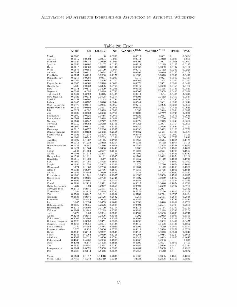
Alleviating NB Attribute Independence Assumption by Attribute Weighting
Table 20: ErrorA1DE LR LR-Reg NB WANBIACLL WANBIAMSE RF100 TAN
Mush 0.0003 0 0 0.0261 0.0012 0.001 0 0.0004Shuttle 0.0012 0.0004 0.0004 0.004 0.0014 0.0012 0.0009 0.001Pioneer 0.0025 0.0079 0.0079 0.0036 0.0002 0.0001 0.0008 0.0057Syncon 0.0033 0.0102 0.0107 0.0133 0.0114 0.0118 0.0127 0.0115Hypo 0.0115 0.0062 0.0049 0.0146 0.0083 0.0082 0.0122 0.0187Wine 0.0174 0.0185 0.0199 0.014 0.0079 0.0112 0.0211 0.0225Anneal 0.0188 0.0117 0.0094 0.0361 0.0199 0.019 0.0122 0.0266Pendigits 0.0197 0.0413 0.0288 0.1179 0.1038 0.1018 0.0339 0.0411Dermatology 0.0213 0.0288 0.031 0.0201 0.019 0.021 0.0367 0.0434Sick 0.0263 0.0269 0.0256 0.0312 0.0263 0.0264 0.0263 0.0272Page-blocks 0.0305 0.0368 0.0318 0.0609 0.0373 0.0351 0.0309 0.0412Optdigits 0.033 0.0533 0.0396 0.0763 0.0642 0.0658 0.0458 0.0487Bcw 0.0371 0.0471 0.0409 0.0266 0.0343 0.0368 0.0386 0.0513Segment 0.0388 0.055 0.0479 0.0752 0.0502 0.0505 0.0413 0.0528Splice-c4.5 0.0404 0.0692 0.045 0.0463 0.0411 0.04 0.0489 0.0613New-thyroid 0.0423 0.0514 0.0528 0.0374 0.0398 0.0412 0.0479 0.0514Musk2 0.0438 0.0207 0.0143 0.0784 0.0399 0.04 0.0385 0.0494Labor 0.0465 0.0737 0.0816 0.0544 0.0544 0.0561 0.0939 0.0842Wall-following 0.0479 0.0118 0.0085 0.0957 0.0219 0.0206 0.0216 0.0693House-votes-84 0.0555 0.0493 0.0461 0.0976 0.0452 0.0463 0.0416 0.0649Iris 0.0577 0.057 0.0573 0.0553 0.053 0.0543 0.056 0.0587Zoo 0.0629 0.0663 0.0683 0.0713 0.0723 0.0757 0.0743 0.0931Spambase 0.0662 0.0626 0.0588 0.0979 0.0626 0.0611 0.0575 0.0689Ionosphere 0.0701 0.0869 0.0818 0.0868 0.0779 0.0746 0.0766 0.0781Nursery 0.0744 0.0747 0.0747 0.0979 0.0979 0.0979 0.0248 0.0686Thyroid 0.0752 0.0683 0.0642 0.1116 0.1061 0.0994 0.075 0.0855Musk1 0.0869 0.0877 0.0811 0.1325 0.0649 0.0666 0.0683 0.0763Kr-vs-kp 0.0915 0.0277 0.0286 0.1267 0.0696 0.0622 0.0128 0.0772Census-income 0.0986 0.0433 0.0433 0.2355 0.0462 0.0461 0.0494 0.0574Letter-recog 0.1025 0.1639 0.1495 0.2563 0.2484 0.2475 0.0902 0.151Car 0.1069 0.0742 0.0733 0.156 0.156 0.156 0.0772 0.081Satellite 0.1092 0.1807 0.1175 0.1751 0.1553 0.1514 0.1085 0.1179Chess 0.1318 0.1233 0.1242 0.1364 0.1338 0.132 0.1074 0.106Waveform-5000 0.1427 0.147 0.1386 0.1918 0.1556 0.1565 0.1558 0.1825Crx 0.1427 0.1564 0.1396 0.1449 0.138 0.1402 0.1581 0.1651Sonar 0.144 0.1784 0.1637 0.1519 0.1688 0.1671 0.1704 0.1683Adult 0.1491 0.1274 0.1274 0.159 0.1306 0.1303 0.1466 0.1387Hungarian 0.1592 0.1811 0.181 0.1585 0.1701 0.1692 0.1874 0.166Hepatitis 0.1619 0.1923 0.17 0.1574 0.1452 0.149 0.1606 0.1713Lyn 0.1669 0.1986 0.1858 0.1666 0.1801 0.1797 0.1909 0.2257Magic 0.1696 0.1538 0.1537 0.2169 0.172 0.1716 0.1674 0.1619Cleveland 0.171 0.1863 0.1766 0.1693 0.1764 0.179 0.1908 0.1909Glass3 0.1724 0.2007 0.1776 0.1871 0.1757 0.1778 0.1951 0.1846Autos 0.1983 0.2154 0.2059 0.2554 0.23 0.2302 0.1937 0.2437Promoters 0.1986 0.1241 0.1302 0.1387 0.1358 0.1363 0.1519 0.2325Horse-colic 0.2107 0.2726 0.1798 0.2126 0.1622 0.1659 0.1789 0.2236Pid 0.2193 0.2197 0.2198 0.2215 0.2151 0.2152 0.2536 0.2249Vowel 0.2199 0.2413 0.2371 0.3931 0.3617 0.3646 0.1674 0.2781Cylinder-bands 0.237 0.24 0.2277 0.2559 0.2591 0.2659 0.2702 0.3761Covtype-mod 0.2413 0.2571 0.2571 0.3117 0.2912 0.2907 0.2512Connect-4 0.244 0.2425 0.2425 0.2792 0.2727 0.2726 0.1875 0.2368Ttt 0.2502 0.0247 0.0181 0.2902 0.2731 0.2714 0.0765 0.2484German 0.2535 0.2575 0.2526 0.2532 0.257 0.2571 0.2684 0.2838Phoneme 0.263 0.2544 0.2068 0.3035 0.2587 0.2607 0.1789 0.3484Led 0.265 0.2694 0.2659 0.2632 0.2633 0.2648 0.2802 0.2702Balance-scale 0.2682 0.2655 0.2626 0.2594 0.2594 0.2594 0.271 0.2661Haberman 0.2714 0.2708 0.2709 0.2714 0.2714 0.2714 0.2709 0.2722Vehicle 0.2761 0.2845 0.2723 0.3765 0.3289 0.3288 0.2742 0.2764Sign 0.279 0.32 0.3204 0.3593 0.3589 0.3568 0.2038 0.2747Audio 0.3288 0.2677 0.2396 0.3305 0.292 0.2942 0.3009 0.3361Volcanoes 0.3309 0.3309 0.3309 0.3309 0.3309 0.3309 0.3309 0.3309Echocardiogram 0.3328 0.3355 0.3351 0.3206 0.3298 0.3302 0.3489 0.3477Contact-lenses 0.3563 0.2958 0.3604 0.3438 0.3417 0.3458 0.3438 0.4292Localization 0.359 0.4584 0.4584 0.4939 0.4902 0.49 0.2976 0.3564Post-operative 0.375 0.425 0.3006 0.3728 0.3611 0.3528 0.3972 0.3706Bupa 0.3843 0.3843 0.3967 0.3843 0.3843 0.3843 0.3817 0.3843Yeast 0.4086 0.4064 0.4059 0.4115 0.4068 0.4084 0.421 0.4096Abalone 0.4562 0.4623 0.4656 0.4794 0.4647 0.4643 0.4823 0.4687Poker-hand 0.4643 0.4988 0.4988 0.4988 0.4988 0.4988 0.329Cmc 0.4791 0.447 0.4478 0.4828 0.4695 0.4654 0.4976 0.465Tae 0.5146 0.5351 0.5334 0.5182 0.5189 0.5096 0.547 0.5344Lung-cancer 0.5281 0.5578 0.5953 0.5203 0.5484 0.5563 0.6 0.4969Ptn 0.5383 0.6444 0.5476 0.5388 0.5456 0.542 0.6 0.5872
Mean 0.1781 0.1817 0.1736 0.2033 0.1886 0.1885 0.1688 0.1890Mean Rank 3.7465 4.5273 3.5000 5.7328 4.2534 4.2808 4.3356 5.6232
39
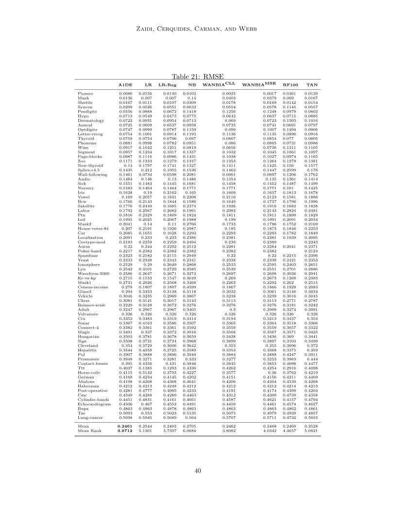
Zaidi, Cerquides, Carman, and Webb
Table 21: RMSEA1DE LR LR-Reg NB WANBIACLL WANBIAMSE RF100 TAN
Pioneer 0.0086 0.0156 0.0140 0.0102 0.0025 0.0017 0.0361 0.0129Mush 0.0136 0.007 0.007 0.14 0.0403 0.0379 0.009 0.0167Shuttle 0.0167 0.0111 0.0107 0.0309 0.0178 0.0169 0.0142 0.0154Syncon 0.0299 0.0526 0.0551 0.0632 0.0554 0.0578 0.1145 0.0557Pendigits 0.0556 0.0888 0.0672 0.1418 0.1256 0.1248 0.0979 0.0802Hypo 0.0713 0.0549 0.0473 0.0775 0.0642 0.0637 0.0715 0.0885Dermatology 0.0722 0.0931 0.0954 0.0713 0.069 0.0723 0.1303 0.1016Anneal 0.0725 0.0609 0.0537 0.0958 0.0735 0.0741 0.0691 0.0797Optdigits 0.0747 0.0999 0.0787 0.1159 0.099 0.1007 0.1494 0.0906Letter-recog 0.0754 0.1001 0.0914 0.1193 0.1136 0.1135 0.0896 0.0916Thyroid 0.0759 0.0754 0.0706 0.097 0.0867 0.0854 0.077 0.0805Phoneme 0.0881 0.0998 0.0782 0.0951 0.086 0.0865 0.0731 0.0986Wine 0.0917 0.1042 0.1251 0.0819 0.0656 0.0736 0.1311 0.1105Segment 0.0957 0.1234 0.1017 0.1357 0.1032 0.1045 0.1061 0.1097Page-blocks 0.0987 0.1116 0.0986 0.1431 0.1038 0.1027 0.0974 0.1165Zoo 0.1171 0.1333 0.1279 0.1247 0.1253 0.1264 0.1279 0.1381New-thyroid 0.14 0.1797 0.1741 0.1327 0.1411 0.1425 0.156 0.1577Splice-c4.5 0.1435 0.212 0.1955 0.1536 0.1462 0.1447 0.2599 0.176Wall-following 0.1461 0.0734 0.0598 0.2081 0.0901 0.0897 0.1206 0.1762Audio 0.1484 0.146 0.13 0.1486 0.1354 0.135 0.1361 0.1414Sick 0.1551 0.1483 0.1445 0.1681 0.1458 0.1452 0.1487 0.1499Nursery 0.1583 0.1464 0.1464 0.1771 0.1771 0.1771 0.101 0.1425Iris 0.1628 0.19 0.2162 0.165 0.1609 0.1637 0.1813 0.1678Vowel 0.169 0.2057 0.1831 0.2206 0.2116 0.2123 0.1581 0.1886Bcw 0.1766 0.2143 0.1844 0.1586 0.1649 0.1737 0.1796 0.1996Satellite 0.1776 0.2449 0.1685 0.2374 0.1926 0.1916 0.1682 0.1838Labor 0.1792 0.2567 0.2682 0.1961 0.2082 0.2143 0.2824 0.2481Ptn 0.1816 0.2329 0.1809 0.1824 0.1811 0.1811 0.1899 0.1829Led 0.1995 0.2025 0.2067 0.1988 0.199 0.1991 0.2091 0.2034Musk2 0.2041 0.14 0.11 0.2766 0.1733 0.1786 0.1752 0.2169House-votes-84 0.207 0.2191 0.1926 0.2987 0.185 0.1873 0.1846 0.2253Car 0.2085 0.1655 0.1628 0.2293 0.2293 0.2293 0.1782 0.1849Localization 0.2091 0.233 0.233 0.2386 0.2381 0.2381 0.1939 0.2095Covtype-mod 0.2183 0.2259 0.2259 0.2494 0.239 0.2389 0.2243Autos 0.22 0.244 0.2202 0.2512 0.2281 0.2284 0.2041 0.2371Poker-hand 0.2217 0.2382 0.2382 0.2382 0.2382 0.2382 0.2124Spambase 0.2323 0.2182 0.2115 0.2949 0.22 0.22 0.2215 0.2396Yeast 0.2333 0.2348 0.2343 0.2341 0.2338 0.2338 0.2421 0.2353Ionosphere 0.2529 0.29 0.2649 0.2868 0.2533 0.2595 0.2403 0.2651Lyn 0.2542 0.3101 0.2729 0.2585 0.2539 0.2551 0.2701 0.2886Waveform-5000 0.2586 0.2647 0.2671 0.3274 0.2697 0.2698 0.3036 0.2941Kr-vs-kp 0.2715 0.1533 0.1547 0.3049 0.269 0.2673 0.1268 0.2383Musk1 0.2731 0.2926 0.2568 0.3468 0.2263 0.2292 0.262 0.2515Census-income 0.278 0.1807 0.1807 0.4599 0.1867 0.1866 0.1928 0.2083Glass3 0.294 0.3453 0.3138 0.3118 0.3032 0.3061 0.3146 0.3034Vehicle 0.3046 0.3235 0.2989 0.3867 0.3238 0.3239 0.3016 0.3045Chess 0.3081 0.3121 0.3017 0.3143 0.3113 0.3113 0.2771 0.2787Balance-scale 0.3229 0.3128 0.3672 0.3276 0.3276 0.3276 0.3181 0.3242Adult 0.3247 0.2967 0.2967 0.3405 0.3 0.2999 0.3274 0.3091Volcanoes 0.326 0.326 0.326 0.326 0.326 0.326 0.326 0.326Crx 0.3353 0.3483 0.3319 0.3414 0.3194 0.3213 0.3437 0.354Sonar 0.3367 0.4163 0.3586 0.3507 0.3365 0.3364 0.3518 0.3366Connect-4 0.3382 0.3361 0.3361 0.3592 0.3559 0.3559 0.3057 0.3322Magic 0.3491 0.337 0.3372 0.3916 0.3568 0.3567 0.3571 0.3425Hungarian 0.3503 0.3781 0.3678 0.3659 0.3428 0.3436 0.369 0.3441Sign 0.3508 0.3731 0.3734 0.3968 0.3899 0.3897 0.3104 0.3499Cleveland 0.354 0.3729 0.3606 0.3642 0.353 0.355 0.3696 0.372Hepatitis 0.3544 0.4358 0.3725 0.3589 0.3353 0.3368 0.3375 0.359Pid 0.3907 0.3888 0.3896 0.3949 0.3884 0.3888 0.4247 0.3911Promoters 0.3948 0.3271 0.3281 0.333 0.3277 0.3253 0.3983 0.444Contact-lenses 0.395 0.4356 0.431 0.3846 0.3845 0.3853 0.4098 0.4477Ttt 0.4037 0.1385 0.1293 0.4336 0.4262 0.4254 0.2916 0.4098Horse-colic 0.4115 0.5142 0.3703 0.4227 0.3577 0.36 0.3762 0.4219German 0.4168 0.4234 0.4145 0.4202 0.4151 0.4156 0.4211 0.4469Abalone 0.4198 0.4208 0.4368 0.4641 0.4206 0.4204 0.4539 0.4268Haberman 0.4212 0.4213 0.4248 0.4212 0.4212 0.4212 0.4214 0.4213Post-operative 0.4281 0.4777 0.4085 0.4233 0.4191 0.4174 0.4399 0.4204Cmc 0.4349 0.4288 0.4289 0.4463 0.4312 0.4309 0.4739 0.4358Cylinder-bands 0.4451 0.4831 0.4161 0.4661 0.4587 0.4621 0.4157 0.4794Echocardiogram 0.4506 0.467 0.4553 0.4491 0.4459 0.4461 0.4574 0.4627Bupa 0.4863 0.4863 0.4878 0.4863 0.4863 0.4863 0.4862 0.4861Tae 0.5093 0.553 0.5023 0.5135 0.5075 0.4979 0.4939 0.4857Lung-cancer 0.5698 0.5945 0.5689 0.564 0.5707 0.5711 0.4732 0.5033
Mean 0.2461 0.2544 0.2403 0.2705 0.2462 0.2468 0.2469 0.2528Mean Rank 3.6712 5.1301 3.7397 6.0684 3.8082 4.0342 4.4657 5.0821
40
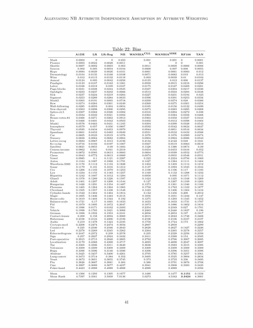
Alleviating NB Attribute Independence Assumption by Attribute Weighting
Table 22: BiasA1DE LR LR-Reg NB WANBIACLL WANBIAMSE RF100 TAN
Mush 0.0002 0 0 0.023 0.001 0.001 0 0.0001Pioneer 0.0003 0.0024 0.0028 0.0011 0 0 0 0.001Shuttle 0.0007 0.0002 0.0003 0.003 0.0011 0.0009 0.0006 0.0006Syncon 0.002 0.005 0.0054 0.0104 0.0068 0.007 0.008 0.0055Hypo 0.0084 0.0029 0.0026 0.0101 0.0061 0.0061 0.0083 0.012Dermatology 0.0104 0.0135 0.0168 0.0108 0.0071 0.0082 0.019 0.013Wine 0.012 0.0115 0.0132 0.0118 0.003 0.0039 0.01 0.0102Anneal 0.0124 0.005 0.0042 0.0256 0.0135 0.012 0.006 0.0137Pendigits 0.0133 0.0167 0.0162 0.1081 0.0939 0.0915 0.0216 0.0296Labor 0.0168 0.0318 0.039 0.0167 0.0175 0.0167 0.0409 0.0201Page-blocks 0.0231 0.0228 0.0244 0.0525 0.0327 0.0304 0.0217 0.0336Optdigits 0.0233 0.0237 0.0232 0.0666 0.0513 0.0503 0.0294 0.0348Sick 0.0237 0.0224 0.0219 0.0284 0.0227 0.0231 0.0194 0.023Segment 0.0253 0.0289 0.0284 0.0633 0.0396 0.0391 0.0253 0.0334Musk2 0.0265 0.0101 0.0065 0.0718 0.0299 0.0274 0.028 0.0386Bcw 0.0274 0.0284 0.0301 0.0249 0.0269 0.0275 0.0301 0.0254Wall-following 0.0285 0.0059 0.004 0.0854 0.0165 0.0156 0.0122 0.0499New-thyroid 0.0303 0.0298 0.0306 0.0295 0.0273 0.0283 0.0285 0.0268Splice-c4.5 0.0307 0.0362 0.0326 0.0382 0.0316 0.0294 0.0272 0.038Zoo 0.0334 0.0332 0.0321 0.0394 0.0363 0.0384 0.0356 0.0468House-votes-84 0.0466 0.0271 0.0262 0.0913 0.0364 0.0358 0.0327 0.0444Iris 0.0466 0.0401 0.0442 0.0503 0.0402 0.0412 0.0398 0.0464Musk1 0.0578 0.0463 0.0431 0.1165 0.0394 0.0399 0.0328 0.0543Ionosphere 0.0579 0.057 0.056 0.0807 0.0592 0.0542 0.0624 0.0647Thyroid 0.0595 0.0434 0.0453 0.0979 0.0944 0.0851 0.0516 0.0634Spambase 0.0601 0.0452 0.0482 0.0949 0.0551 0.0532 0.0432 0.0588Car 0.0605 0.0523 0.0519 0.1076 0.1076 0.1076 0.0389 0.0474Nursery 0.0656 0.0684 0.0682 0.0904 0.0904 0.0904 0.0086 0.0543Letter-recog 0.0684 0.0967 0.1013 0.2196 0.2134 0.2122 0.049 0.1041Kr-vs-kp 0.0716 0.0192 0.0197 0.1067 0.0567 0.0519 0.0063 0.0619Satellite 0.0831 0.0855 0.09 0.1684 0.1428 0.1386 0.0874 0.09Census-income 0.0862 0.041 0.041 0.2319 0.0454 0.0453 0.0416 0.052Promoters 0.0872 0.0585 0.0613 0.0683 0.0604 0.0599 0.0552 0.0773Chess 0.0943 0.0772 0.0813 0.0989 0.0974 0.0955 0.0548 0.0551Vowel 0.0985 0.1 0.1121 0.2287 0.222 0.2224 0.0756 0.1069Autos 0.1164 0.1087 0.1068 0.1791 0.1427 0.1384 0.1111 0.1464Waveform-5000 0.1176 0.1112 0.1134 0.1828 0.1404 0.1403 0.1114 0.1212Sonar 0.1179 0.101 0.1016 0.1314 0.1137 0.1094 0.1045 0.1044Crx 0.1206 0.1103 0.1079 0.1253 0.1108 0.1106 0.117 0.1185Lyn 0.1234 0.1155 0.1183 0.1257 0.1169 0.1132 0.1288 0.1232Hepatitis 0.1242 0.1007 0.1012 0.1294 0.0958 0.095 0.1071 0.1112Glass3 0.1378 0.1289 0.1226 0.1597 0.1424 0.1425 0.1348 0.1269Adult 0.1401 0.1207 0.1208 0.1544 0.127 0.1267 0.1109 0.1263Hungarian 0.1426 0.1291 0.1354 0.1487 0.1373 0.1361 0.1346 0.1166Phoneme 0.1465 0.1264 0.1264 0.1965 0.1758 0.1763 0.1102 0.1877Cleveland 0.1505 0.1357 0.1438 0.1548 0.1423 0.1406 0.1304 0.1416Cylinder-bands 0.1522 0.1464 0.1464 0.1814 0.142 0.1456 0.208 0.2912Magic 0.1605 0.1446 0.1443 0.2115 0.1656 0.1651 0.1244 0.147Horse-colic 0.1619 0.1403 0.1344 0.182 0.1275 0.1293 0.1345 0.1452Balance-scale 0.1721 0.17 0.1665 0.1633 0.1633 0.1633 0.1731 0.1707Pid 0.1979 0.1895 0.1872 0.2047 0.1873 0.1886 0.1802 0.1816Ttt 0.1996 0.0171 0.0162 0.2493 0.2354 0.2349 0.027 0.1701Vehicle 0.1998 0.1765 0.1821 0.3066 0.2463 0.2446 0.1827 0.196German 0.1998 0.1932 0.1953 0.2101 0.2058 0.2053 0.197 0.1917Contact-lenses 0.209 0.158 0.2094 0.2069 0.2015 0.2042 0.1748 0.3408Haberman 0.2106 0.2124 0.2206 0.2106 0.2106 0.2106 0.2107 0.2107Audio 0.219 0.1478 0.1424 0.2185 0.1758 0.1744 0.173 0.1662Covtype-mod 0.2208 0.2474 0.2474 0.3034 0.2867 0.2858 0.2299Connect-4 0.225 0.2346 0.2346 0.2643 0.2628 0.2627 0.1427 0.2226Led 0.2278 0.2269 0.2245 0.2262 0.2264 0.2265 0.2278 0.2257Echocardiogram 0.2447 0.2372 0.239 0.2578 0.235 0.2329 0.2256 0.2356Sign 0.257 0.2927 0.2924 0.3432 0.3411 0.3388 0.154 0.2505Post-operative 0.2915 0.2715 0.2848 0.2805 0.2792 0.2766 0.3007 0.2685Localization 0.3179 0.4368 0.4368 0.4717 0.4693 0.4698 0.2047 0.3097Tae 0.3305 0.3306 0.3311 0.3649 0.3636 0.3583 0.3315 0.3385Volcanoes 0.3309 0.3309 0.3309 0.3309 0.3309 0.3309 0.3309 0.3309Bupa 0.3396 0.3396 0.3146 0.3396 0.3396 0.3396 0.3451 0.3396Abalone 0.3425 0.3457 0.3406 0.4201 0.3795 0.3785 0.3257 0.3361Lung-cancer 0.3473 0.3714 0.384 0.352 0.3495 0.3525 0.3804 0.2834Yeast 0.3672 0.3651 0.3655 0.3745 0.373 0.3722 0.336 0.3495Ptn 0.3826 0.3667 0.3681 0.384 0.386 0.3791 0.3876 0.3708Cmc 0.3907 0.3689 0.3677 0.4237 0.3941 0.3908 0.3383 0.3425Poker-hand 0.4423 0.4988 0.4988 0.4988 0.4988 0.4988 0.2356
Mean 0.1366 0.1293 0.1305 0.1677 0.1486 0.1477 0.1151 0.1334Mean Rank 4.7397 3.3561 3.5958 7.0136 5.0273 4.5342 3.3424 4.3901
41
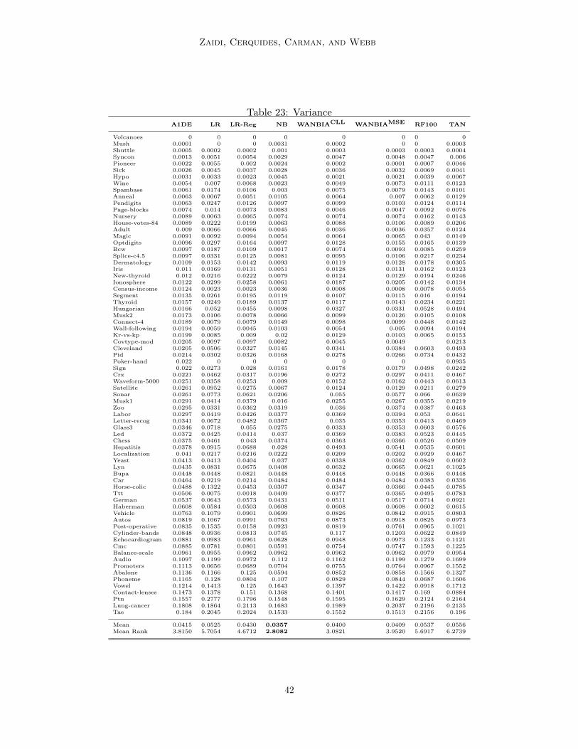
Zaidi, Cerquides, Carman, and Webb
Table 23: VarianceA1DE LR LR-Reg NB WANBIACLL WANBIAMSE RF100 TAN
Volcanoes 0 0 0 0 0 0 0 0Mush 0.0001 0 0 0.0031 0.0002 0 0 0.0003Shuttle 0.0005 0.0002 0.0002 0.001 0.0003 0.0003 0.0003 0.0004Syncon 0.0013 0.0051 0.0054 0.0029 0.0047 0.0048 0.0047 0.006Pioneer 0.0022 0.0055 0.002 0.0024 0.0002 0.0001 0.0007 0.0046Sick 0.0026 0.0045 0.0037 0.0028 0.0036 0.0032 0.0069 0.0041Hypo 0.0031 0.0033 0.0023 0.0045 0.0021 0.0021 0.0039 0.0067Wine 0.0054 0.007 0.0068 0.0023 0.0049 0.0073 0.0111 0.0123Spambase 0.0061 0.0174 0.0106 0.003 0.0075 0.0079 0.0143 0.0101Anneal 0.0063 0.0067 0.0051 0.0105 0.0064 0.007 0.0062 0.0129Pendigits 0.0063 0.0247 0.0126 0.0097 0.0099 0.0103 0.0124 0.0114Page-blocks 0.0074 0.014 0.0073 0.0083 0.0046 0.0047 0.0092 0.0076Nursery 0.0089 0.0063 0.0065 0.0074 0.0074 0.0074 0.0162 0.0143House-votes-84 0.0089 0.0222 0.0199 0.0063 0.0088 0.0106 0.0089 0.0206Adult 0.009 0.0066 0.0066 0.0045 0.0036 0.0036 0.0357 0.0124Magic 0.0091 0.0092 0.0094 0.0054 0.0064 0.0065 0.043 0.0149Optdigits 0.0096 0.0297 0.0164 0.0097 0.0128 0.0155 0.0165 0.0139Bcw 0.0097 0.0187 0.0109 0.0017 0.0074 0.0093 0.0085 0.0259Splice-c4.5 0.0097 0.0331 0.0125 0.0081 0.0095 0.0106 0.0217 0.0234Dermatology 0.0109 0.0153 0.0142 0.0093 0.0119 0.0128 0.0178 0.0305Iris 0.011 0.0169 0.0131 0.0051 0.0128 0.0131 0.0162 0.0123New-thyroid 0.012 0.0216 0.0222 0.0079 0.0124 0.0129 0.0194 0.0246Ionosphere 0.0122 0.0299 0.0258 0.0061 0.0187 0.0205 0.0142 0.0134Census-income 0.0124 0.0023 0.0023 0.0036 0.0008 0.0008 0.0078 0.0055Segment 0.0135 0.0261 0.0195 0.0119 0.0107 0.0115 0.016 0.0194Thyroid 0.0157 0.0249 0.0189 0.0137 0.0117 0.0143 0.0234 0.0221Hungarian 0.0166 0.052 0.0455 0.0098 0.0327 0.0331 0.0528 0.0494Musk2 0.0173 0.0106 0.0078 0.0066 0.0099 0.0126 0.0105 0.0108Connect-4 0.0189 0.0079 0.0079 0.0149 0.0098 0.0099 0.0448 0.0142Wall-following 0.0194 0.0059 0.0045 0.0103 0.0054 0.005 0.0094 0.0194Kr-vs-kp 0.0199 0.0085 0.009 0.02 0.0129 0.0103 0.0065 0.0153Covtype-mod 0.0205 0.0097 0.0097 0.0082 0.0045 0.0049 0.0213Cleveland 0.0205 0.0506 0.0327 0.0145 0.0341 0.0384 0.0603 0.0493Pid 0.0214 0.0302 0.0326 0.0168 0.0278 0.0266 0.0734 0.0432Poker-hand 0.022 0 0 0 0 0 0.0935Sign 0.022 0.0273 0.028 0.0161 0.0178 0.0179 0.0498 0.0242Crx 0.0221 0.0462 0.0317 0.0196 0.0272 0.0297 0.0411 0.0467Waveform-5000 0.0251 0.0358 0.0253 0.009 0.0152 0.0162 0.0443 0.0613Satellite 0.0261 0.0952 0.0275 0.0067 0.0124 0.0129 0.0211 0.0279Sonar 0.0261 0.0773 0.0621 0.0206 0.055 0.0577 0.066 0.0639Musk1 0.0291 0.0414 0.0379 0.016 0.0255 0.0267 0.0355 0.0219Zoo 0.0295 0.0331 0.0362 0.0319 0.036 0.0374 0.0387 0.0463Labor 0.0297 0.0419 0.0426 0.0377 0.0369 0.0394 0.053 0.0641Letter-recog 0.0341 0.0672 0.0482 0.0367 0.035 0.0353 0.0413 0.0469Glass3 0.0346 0.0718 0.055 0.0275 0.0333 0.0353 0.0603 0.0576Led 0.0372 0.0425 0.0414 0.037 0.0369 0.0383 0.0523 0.0445Chess 0.0375 0.0461 0.043 0.0374 0.0363 0.0366 0.0526 0.0509Hepatitis 0.0378 0.0915 0.0688 0.028 0.0493 0.0541 0.0535 0.0601Localization 0.041 0.0217 0.0216 0.0222 0.0209 0.0202 0.0929 0.0467Yeast 0.0413 0.0413 0.0404 0.037 0.0338 0.0362 0.0849 0.0602Lyn 0.0435 0.0831 0.0675 0.0408 0.0632 0.0665 0.0621 0.1025Bupa 0.0448 0.0448 0.0821 0.0448 0.0448 0.0448 0.0366 0.0448Car 0.0464 0.0219 0.0214 0.0484 0.0484 0.0484 0.0383 0.0336Horse-colic 0.0488 0.1322 0.0453 0.0307 0.0347 0.0366 0.0445 0.0785Ttt 0.0506 0.0075 0.0018 0.0409 0.0377 0.0365 0.0495 0.0783German 0.0537 0.0643 0.0573 0.0431 0.0511 0.0517 0.0714 0.0921Haberman 0.0608 0.0584 0.0503 0.0608 0.0608 0.0608 0.0602 0.0615Vehicle 0.0763 0.1079 0.0901 0.0699 0.0826 0.0842 0.0915 0.0803Autos 0.0819 0.1067 0.0991 0.0763 0.0873 0.0918 0.0825 0.0973Post-operative 0.0835 0.1535 0.0158 0.0923 0.0819 0.0761 0.0965 0.1021Cylinder-bands 0.0848 0.0936 0.0813 0.0745 0.117 0.1203 0.0622 0.0849Echocardiogram 0.0881 0.0983 0.0961 0.0628 0.0948 0.0973 0.1233 0.1121Cmc 0.0885 0.0781 0.0801 0.0591 0.0754 0.0747 0.1593 0.1225Balance-scale 0.0961 0.0955 0.0962 0.0962 0.0962 0.0962 0.0979 0.0954Audio 0.1097 0.1199 0.0972 0.112 0.1162 0.1199 0.1279 0.1699Promoters 0.1113 0.0656 0.0689 0.0704 0.0755 0.0764 0.0967 0.1552Abalone 0.1136 0.1166 0.125 0.0594 0.0852 0.0858 0.1566 0.1327Phoneme 0.1165 0.128 0.0804 0.107 0.0829 0.0844 0.0687 0.1606Vowel 0.1214 0.1413 0.125 0.1643 0.1397 0.1422 0.0918 0.1712Contact-lenses 0.1473 0.1378 0.151 0.1368 0.1401 0.1417 0.169 0.0884Ptn 0.1557 0.2777 0.1796 0.1548 0.1595 0.1629 0.2124 0.2164Lung-cancer 0.1808 0.1864 0.2113 0.1683 0.1989 0.2037 0.2196 0.2135Tae 0.184 0.2045 0.2024 0.1533 0.1552 0.1513 0.2156 0.196
Mean 0.0415 0.0525 0.0430 0.0357 0.0400 0.0409 0.0537 0.0556Mean Rank 3.8150 5.7054 4.6712 2.8082 3.0821 3.9520 5.6917 6.2739
42
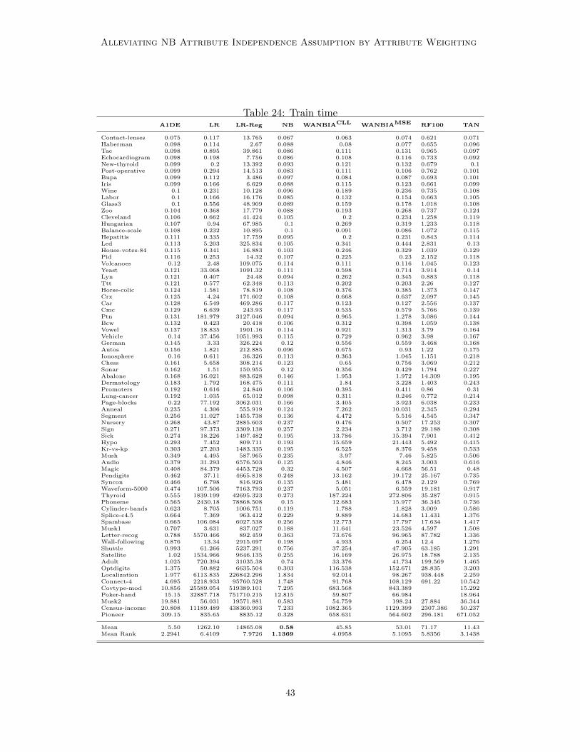
Alleviating NB Attribute Independence Assumption by Attribute Weighting
Table 24: Train timeA1DE LR LR-Reg NB WANBIACLL WANBIAMSE RF100 TAN
Contact-lenses 0.075 0.117 13.765 0.067 0.063 0.074 0.621 0.071Haberman 0.098 0.114 2.67 0.088 0.08 0.077 0.655 0.096Tae 0.098 0.895 39.861 0.086 0.111 0.131 0.965 0.097Echocardiogram 0.098 0.198 7.756 0.086 0.108 0.116 0.733 0.092New-thyroid 0.099 0.2 13.392 0.093 0.121 0.132 0.679 0.1Post-operative 0.099 0.294 14.513 0.083 0.111 0.106 0.762 0.101Bupa 0.099 0.112 3.486 0.097 0.084 0.087 0.693 0.101Iris 0.099 0.166 6.629 0.088 0.115 0.123 0.661 0.099Wine 0.1 0.231 10.128 0.096 0.189 0.236 0.735 0.108Labor 0.1 0.166 16.176 0.085 0.132 0.154 0.663 0.105Glass3 0.1 0.556 48.909 0.089 0.159 0.178 1.018 0.108Zoo 0.104 0.368 17.779 0.088 0.193 0.268 0.737 0.124Cleveland 0.106 0.662 41.424 0.105 0.2 0.234 1.258 0.119Hungarian 0.107 0.94 67.985 0.1 0.269 0.319 1.233 0.118Balance-scale 0.108 0.232 10.895 0.1 0.091 0.086 1.072 0.115Hepatitis 0.111 0.335 17.759 0.095 0.2 0.231 0.843 0.114Led 0.113 5.203 325.834 0.105 0.341 0.444 2.831 0.13House-votes-84 0.115 0.341 16.883 0.103 0.246 0.329 1.039 0.129Pid 0.116 0.253 14.32 0.107 0.225 0.23 2.152 0.118Volcanoes 0.12 2.48 109.075 0.114 0.111 0.116 1.045 0.123Yeast 0.121 33.068 1091.32 0.111 0.598 0.714 3.914 0.14Lyn 0.121 0.407 24.48 0.094 0.262 0.345 0.883 0.118Ttt 0.121 0.577 62.348 0.113 0.202 0.203 2.26 0.127Horse-colic 0.124 1.581 78.819 0.108 0.376 0.385 1.373 0.147Crx 0.125 4.24 171.602 0.108 0.668 0.637 2.097 0.145Car 0.128 6.549 469.286 0.117 0.123 0.127 2.556 0.137Cmc 0.129 6.639 243.93 0.117 0.535 0.579 5.766 0.139Ptn 0.131 181.979 3127.046 0.094 0.965 1.278 3.086 0.144Bcw 0.132 0.423 20.418 0.106 0.312 0.398 1.059 0.138Vowel 0.137 18.835 1901.16 0.114 0.921 1.313 3.79 0.164Vehicle 0.14 37.456 1051.993 0.115 0.729 0.962 3.98 0.167German 0.145 3.33 326.224 0.12 0.556 0.559 3.468 0.168Autos 0.156 1.821 212.885 0.096 0.675 0.93 1.22 0.175Ionosphere 0.16 0.611 36.326 0.113 0.363 1.045 1.151 0.218Chess 0.161 5.658 308.214 0.123 0.65 0.756 3.069 0.212Sonar 0.162 1.51 150.955 0.12 0.356 0.429 1.794 0.227Abalone 0.168 16.021 883.628 0.146 1.953 1.972 14.309 0.195Dermatology 0.183 1.792 168.475 0.111 1.84 3.228 1.403 0.243Promoters 0.192 0.616 24.846 0.106 0.395 0.411 0.86 0.31Lung-cancer 0.192 1.035 65.012 0.098 0.311 0.246 0.772 0.214Page-blocks 0.22 77.192 3062.031 0.166 3.405 3.923 6.038 0.233Anneal 0.235 4.306 555.919 0.124 7.262 10.031 2.345 0.294Segment 0.256 11.027 1455.738 0.136 4.472 5.516 4.545 0.347Nursery 0.268 43.87 2885.603 0.237 0.476 0.507 17.253 0.307Sign 0.271 97.373 3309.138 0.257 2.234 3.712 29.188 0.308Sick 0.274 18.226 1497.482 0.195 13.786 15.394 7.901 0.412Hypo 0.293 7.452 809.711 0.193 15.659 21.443 5.492 0.415Kr-vs-kp 0.303 27.203 1483.335 0.195 6.525 8.376 9.458 0.533Mush 0.349 4.495 587.965 0.235 3.97 7.46 5.825 0.506Audio 0.379 31.293 6576.503 0.125 4.846 8.245 3.003 0.616Magic 0.408 84.379 4453.728 0.32 4.507 4.668 56.51 0.48Pendigits 0.462 37.11 4665.818 0.248 13.162 19.172 25.167 0.735Syncon 0.466 6.798 816.926 0.135 5.481 6.478 2.129 0.769Waveform-5000 0.474 107.506 7163.793 0.237 5.051 6.559 19.181 0.917Thyroid 0.555 1839.199 42695.323 0.273 187.224 272.806 35.287 0.915Phoneme 0.565 2430.18 78868.508 0.15 12.683 15.977 36.345 0.736Cylinder-bands 0.623 8.705 1006.751 0.119 1.788 1.828 3.009 0.586Splice-c4.5 0.664 7.369 963.412 0.229 9.889 14.683 11.431 1.376Spambase 0.665 106.084 6027.538 0.256 12.773 17.797 17.634 1.417Musk1 0.707 3.631 837.027 0.188 11.641 23.526 4.597 1.508Letter-recog 0.788 5570.466 892.459 0.363 73.676 96.965 87.782 1.336Wall-following 0.876 13.34 2915.697 0.198 4.933 6.254 12.4 1.276Shuttle 0.993 61.266 5237.291 0.756 37.254 47.905 63.185 1.291Satellite 1.02 1534.966 9646.135 0.255 16.169 26.975 18.788 2.135Adult 1.025 720.394 31035.38 0.74 33.376 41.734 199.569 1.465Optdigits 1.375 50.882 6635.504 0.303 116.538 152.671 28.835 3.203Localization 1.977 6113.835 226842.296 1.834 92.014 98.267 938.448 2.259Connect-4 4.695 2218.933 95760.528 1.748 91.768 108.129 691.22 10.542Covtype-mod 10.856 25589.054 519389.101 7.295 683.568 843.389 15.292Poker-hand 15.15 32887.718 751710.215 12.815 59.807 66.984 18.964Musk2 19.881 56.031 19571.881 0.583 54.759 198.24 27.884 36.344Census-income 20.808 11189.489 438360.993 7.233 1082.365 1129.399 2307.386 50.237Pioneer 309.15 835.65 8835.12 0.328 658.631 564.602 296.181 671.052
Mean 5.50 1262.10 14865.08 0.58 45.85 53.01 71.17 11.43Mean Rank 2.2941 6.4109 7.9726 1.1369 4.0958 5.1095 5.8356 3.1438
43
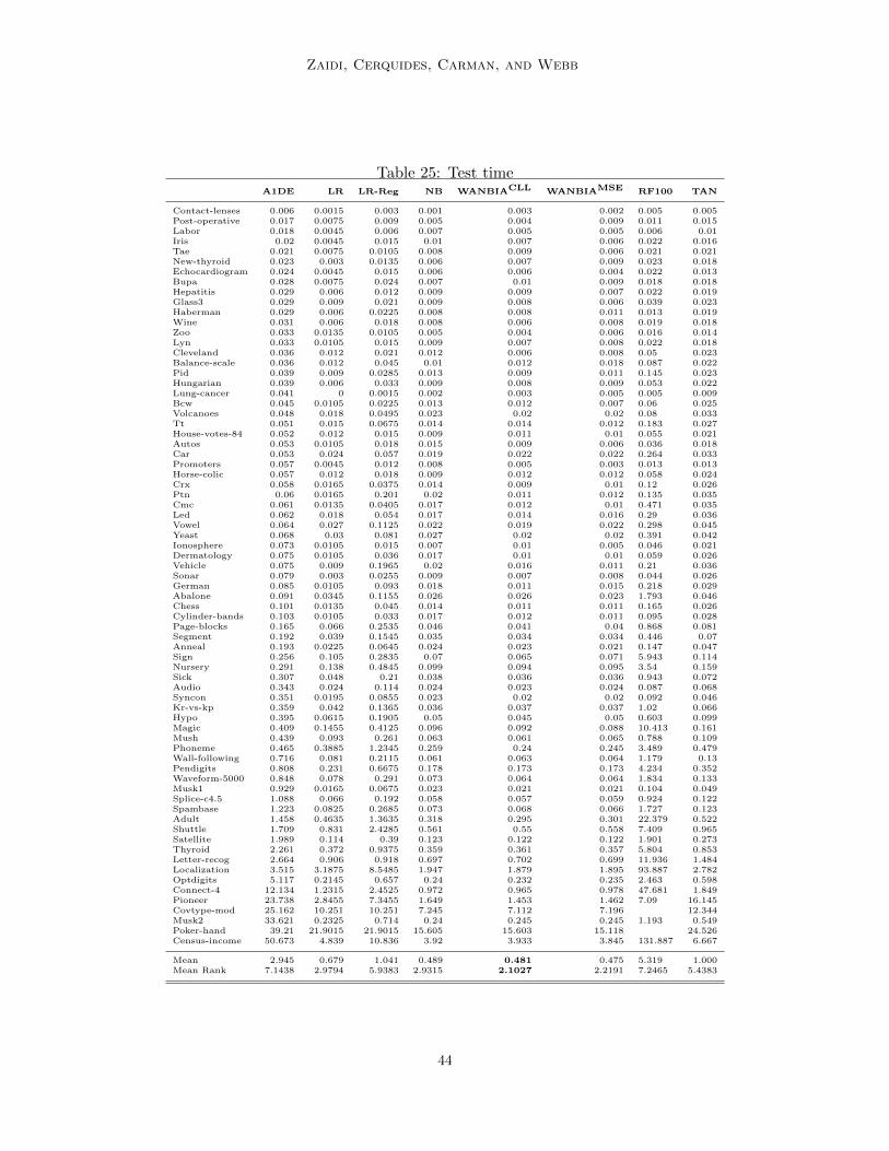
Zaidi, Cerquides, Carman, and Webb
Table 25: Test timeA1DE LR LR-Reg NB WANBIACLL WANBIAMSE RF100 TAN
Contact-lenses 0.006 0.0015 0.003 0.001 0.003 0.002 0.005 0.005Post-operative 0.017 0.0075 0.009 0.005 0.004 0.009 0.011 0.015Labor 0.018 0.0045 0.006 0.007 0.005 0.005 0.006 0.01Iris 0.02 0.0045 0.015 0.01 0.007 0.006 0.022 0.016Tae 0.021 0.0075 0.0105 0.008 0.009 0.006 0.021 0.021New-thyroid 0.023 0.003 0.0135 0.006 0.007 0.009 0.023 0.018Echocardiogram 0.024 0.0045 0.015 0.006 0.006 0.004 0.022 0.013Bupa 0.028 0.0075 0.024 0.007 0.01 0.009 0.018 0.018Hepatitis 0.029 0.006 0.012 0.009 0.009 0.007 0.022 0.019Glass3 0.029 0.009 0.021 0.009 0.008 0.006 0.039 0.023Haberman 0.029 0.006 0.0225 0.008 0.008 0.011 0.013 0.019Wine 0.031 0.006 0.018 0.008 0.006 0.008 0.019 0.018Zoo 0.033 0.0135 0.0105 0.005 0.004 0.006 0.016 0.014Lyn 0.033 0.0105 0.015 0.009 0.007 0.008 0.022 0.018Cleveland 0.036 0.012 0.021 0.012 0.006 0.008 0.05 0.023Balance-scale 0.036 0.012 0.045 0.01 0.012 0.018 0.087 0.022Pid 0.039 0.009 0.0285 0.013 0.009 0.011 0.145 0.023Hungarian 0.039 0.006 0.033 0.009 0.008 0.009 0.053 0.022Lung-cancer 0.041 0 0.0015 0.002 0.003 0.005 0.005 0.009Bcw 0.045 0.0105 0.0225 0.013 0.012 0.007 0.06 0.025Volcanoes 0.048 0.018 0.0495 0.023 0.02 0.02 0.08 0.033Tt 0.051 0.015 0.0675 0.014 0.014 0.012 0.183 0.027House-votes-84 0.052 0.012 0.015 0.009 0.011 0.01 0.055 0.021Autos 0.053 0.0105 0.018 0.015 0.009 0.006 0.036 0.018Car 0.053 0.024 0.057 0.019 0.022 0.022 0.264 0.033Promoters 0.057 0.0045 0.012 0.008 0.005 0.003 0.013 0.013Horse-colic 0.057 0.012 0.018 0.009 0.012 0.012 0.058 0.024Crx 0.058 0.0165 0.0375 0.014 0.009 0.01 0.12 0.026Ptn 0.06 0.0165 0.201 0.02 0.011 0.012 0.135 0.035Cmc 0.061 0.0135 0.0405 0.017 0.012 0.01 0.471 0.035Led 0.062 0.018 0.054 0.017 0.014 0.016 0.29 0.036Vowel 0.064 0.027 0.1125 0.022 0.019 0.022 0.298 0.045Yeast 0.068 0.03 0.081 0.027 0.02 0.02 0.391 0.042Ionosphere 0.073 0.0105 0.015 0.007 0.01 0.005 0.046 0.021Dermatology 0.075 0.0105 0.036 0.017 0.01 0.01 0.059 0.026Vehicle 0.075 0.009 0.1965 0.02 0.016 0.011 0.21 0.036Sonar 0.079 0.003 0.0255 0.009 0.007 0.008 0.044 0.026German 0.085 0.0105 0.093 0.018 0.011 0.015 0.218 0.029Abalone 0.091 0.0345 0.1155 0.026 0.026 0.023 1.793 0.046Chess 0.101 0.0135 0.045 0.014 0.011 0.011 0.165 0.026Cylinder-bands 0.103 0.0105 0.033 0.017 0.012 0.011 0.095 0.028Page-blocks 0.165 0.066 0.2535 0.046 0.041 0.04 0.868 0.081Segment 0.192 0.039 0.1545 0.035 0.034 0.034 0.446 0.07Anneal 0.193 0.0225 0.0645 0.024 0.023 0.021 0.147 0.047Sign 0.256 0.105 0.2835 0.07 0.065 0.071 5.943 0.114Nursery 0.291 0.138 0.4845 0.099 0.094 0.095 3.54 0.159Sick 0.307 0.048 0.21 0.038 0.036 0.036 0.943 0.072Audio 0.343 0.024 0.114 0.024 0.023 0.024 0.087 0.068Syncon 0.351 0.0195 0.0855 0.023 0.02 0.02 0.092 0.046Kr-vs-kp 0.359 0.042 0.1365 0.036 0.037 0.037 1.02 0.066Hypo 0.395 0.0615 0.1905 0.05 0.045 0.05 0.603 0.099Magic 0.409 0.1455 0.4125 0.096 0.092 0.088 10.413 0.161Mush 0.439 0.093 0.261 0.063 0.061 0.065 0.788 0.109Phoneme 0.465 0.3885 1.2345 0.259 0.24 0.245 3.489 0.479Wall-following 0.716 0.081 0.2115 0.061 0.063 0.064 1.179 0.13Pendigits 0.808 0.231 0.6675 0.178 0.173 0.173 4.234 0.352Waveform-5000 0.848 0.078 0.291 0.073 0.064 0.064 1.834 0.133Musk1 0.929 0.0165 0.0675 0.023 0.021 0.021 0.104 0.049Splice-c4.5 1.088 0.066 0.192 0.058 0.057 0.059 0.924 0.122Spambase 1.223 0.0825 0.2685 0.073 0.068 0.066 1.727 0.123Adult 1.458 0.4635 1.3635 0.318 0.295 0.301 22.379 0.522Shuttle 1.709 0.831 2.4285 0.561 0.55 0.558 7.409 0.965Satellite 1.989 0.114 0.39 0.123 0.122 0.122 1.901 0.273Thyroid 2.261 0.372 0.9375 0.359 0.361 0.357 5.804 0.853Letter-recog 2.664 0.906 0.918 0.697 0.702 0.699 11.936 1.484Localization 3.515 3.1875 8.5485 1.947 1.879 1.895 93.887 2.782Optdigits 5.117 0.2145 0.657 0.24 0.232 0.235 2.463 0.598Connect-4 12.134 1.2315 2.4525 0.972 0.965 0.978 47.681 1.849Pioneer 23.738 2.8455 7.3455 1.649 1.453 1.462 7.09 16.145Covtype-mod 25.162 10.251 10.251 7.245 7.112 7.196 12.344Musk2 33.621 0.2325 0.714 0.24 0.245 0.245 1.193 0.549Poker-hand 39.21 21.9015 21.9015 15.605 15.603 15.118 24.526Census-income 50.673 4.839 10.836 3.92 3.933 3.845 131.887 6.667
Mean 2.945 0.679 1.041 0.489 0.481 0.475 5.319 1.000Mean Rank 7.1438 2.9794 5.9383 2.9315 2.1027 2.2191 7.2465 5.4383
44