Embed Size (px)
Citation preview

AM111 DocumentationRelease 0.1
Jiawei Zhuang
Nov 22, 2017


Contents
1 Homework Notes 3
2 Lecture & Session Notes 7
3 MATLAB in Jupyter Notebooks 89
i

ii
AM111 Documentation, Release 0.1
Course Name: Applied Math 111, Introduction to Scientific Computing
Instructor: Prof. Robin Wordsworth ([email protected]), 426 Geological MuseumTeaching Fellow: Jiawei Zhuang ([email protected]), Pierce Hall 108
Lecture Time: Tues/Thurs 13:00-14:30Lecture Location: 375 Geological Museum (3rd floor)
Session Time: Every Monday 17:00-18:00Session Location: GeoMuseum 103A
TF’s Office Hour: Every Tuesday 15:00-16:00, Pierce Hall 108
This website contains supplemental materials made by the TF, Jiawei Zhuang. These materials are not required forcompleting this course, but just provide additional information I find useful. Might also use them for the session. Yourgrade will not be affected if you choose to ignore this website.
Contents 1

AM111 Documentation, Release 0.1
2 Contents
CHAPTER 1
Homework Notes
Additional notes (hints, clarifications) for homework.
1.1 Notes on Homework 1
In [1]: format compact
The last question asks you to use boolean_print_TT_fn.m (available on canvas) to print the truth table. Please readthis additional note if you have trouble using this function.
1.1.1 Function as an input variable
Typically you pass data (e.g. scalars, arrays. . . ) to a function. But the function boolean_print_TT_fn() acceptsanother function as the input variable.
Inline function as an input variable
Let’s make two inline functions:
In [2]: func1 = @(a) a;func2 = @(a,b) a&b;
boolean_print_TT_fn(func,1) prints the truth table for a function with a single input:
In [3]: boolean_print_TT_fn(func1,1)
_____a|out0|01|1
boolean_print_TT_fn(func,2) prints the truth table for a function with two inputs:
In [4]: boolean_print_TT_fn(func2,2)
3
AM111 Documentation, Release 0.1
_______a|b|out0|0| 00|1| 01|0| 01|1| 1
Standard function as an input variable
However, if you try to pass a standard function (i.e. defined in a separate file) to boolean_print_TT_fn(), itwill throw you some weird error:
In [5]: %%file func2_fn.mfunction s=func2_fn(a,b)
s = a&b;end
Created file '/Users/zhuangjw/Research/Computing/personal_web/AM111/docs/func2_fn.m'.
In [6]: boolean_print_TT_fn(func2_fn,2)
Not enough input arguments.Error in func2_fn (line 2) s = a&b;
To fix this error, you can put @ in front of your function, as suggested here.
In [7]: boolean_print_TT_fn(@func2_fn,2)
_______a|b|out0|0| 00|1| 01|0| 01|1| 1
(That’s MATLAB-specific design. Other languages like Python treat inline and standard functions in the same way.)
1.1.2 Print truth table for half adder
Function with multiple return
A Half adder has two return values. One way to return multiple values is
In [8]: %%file multi_return.mfunction [carry,s] = multi_return(a,b)
% This is not a corret adder! You should write your own!carry = 0;s = 1;
end
Created file '/Users/zhuangjw/Research/Computing/personal_web/AM111/docs/multi_return.m'.
However, by default you only get the first output variable carry !
In [9]: multi_return(0,0)
ans =0
To get both carry and s, you have to use two variables to hold the output results.
In [10]: [out1, out2] = multi_return(0,0)
4 Chapter 1. Homework Notes
AM111 Documentation, Release 0.1
out1 =0
out2 =1
A perhaps more convenient way is to return a vector containing all outputs you need:
In [11]: %%file fake_half_adder.mfunction out = fake_half_adder(a,b)
% This is not a corret adder! You should write your own!carry = 0;s = 1;out = [carry,s];
end
Created file '/Users/zhuangjw/Research/Computing/personal_web/AM111/docs/fake_half_adder.m'.
This time, you don’t have to write two variables to hold the output results:
In [12]: fake_half_adder(1,1)
ans =0 1
Print truth table using boolean_print_TT_fn.m
boolean_print_TT_fn() will print the complete result only if you use a single vector as the return value for youadder. Use 3 to get the format for half-adder.
In [13]: boolean_print_TT_fn(@multi_return,3) % not printing complete result
_____________a|b|carry|sum0|0| 00|1| 01|0| 01|1| 0
In [14]: boolean_print_TT_fn(@fake_half_adder,3) % can print complete result
_____________a|b|carry|sum0|0| 0 10|1| 0 11|0| 0 11|1| 0 1
Print truth table on your own
If you don’t want to use boolean_print_TT_fn.m, it is also quite straightforward to print the table on your own:
In [15]: disp('a,b|c,s')for a=0:1for b=0:1
fprintf('%d,%d|%d,%d \n',a,b,fake_half_adder(a,b))endend
a,b|c,s0,0|0,10,1|0,1
1.1. Notes on Homework 1 5

AM111 Documentation, Release 0.1
1,0|0,11,1|0,1
Type doc fprintf to see more formatting options.
1.1.3 Print truth table for full adder
Use 4 to get the format for full-adder.
In [16]: %%file fake_full_adder.mfunction out = fake_full_adder(a,b,c)
carry = 0;s = 1;out = [carry,s];
end
Created file '/Users/zhuangjw/Research/Computing/personal_web/AM111/docs/fake_full_adder.m'.
In [17]: boolean_print_TT_fn(@fake_full_adder,4)
________________a|b|c|carry|sum0|0|0|0 10|0|1|0 10|1|0|0 10|1|1|0 11|0|0|0 11|0|1|0 11|1|0|0 11|1|1|0 1
6 Chapter 1. Homework Notes
CHAPTER 2
Lecture & Session Notes
Forget the coding exercises in the class? The following notes might help.
2.1 Lecture 2: Logic Gates & Fibonacci Numbers
Date: 09/05/2017, Tuesday
In [1]: format compact
2.1.1 Logic gates
nand gate
In [2]: nand = @(a,b) ~(a&b)
nand =function_handle with value:@(a,b)~(a&b)
In [3]: nand(1,1) % test if it works
ans =logical0
print truth table
In [4]: help boolean_print_TT_fn % boolean_print_TT_fn.m is available on canvas
boolean_print_TT_fn.ma function to print the boolean truth table for a givensupplied function 'func'
7

AM111 Documentation, Release 0.1
INPUTfunc: the supplied function (e.g. OR, NAND, XOR)input_num: number of inputs
In [5]: boolean_print_TT_fn(nand,2)
_______a|b|out0|0| 10|1| 11|0| 11|1| 0
build “not” gate from “nand” gate
In [6]: my_not = @(a) nand(a,a) % "not" is a built-in function so we use my_not to avoid conflicts
my_not =function_handle with value:@(a)nand(a,a)
In [7]: boolean_print_TT_fn(my_not,1)
_____a|out0|11|0
Why nand(a,a) means not:
1. and(a,a) = a, no matter a is 0 or 1
2. nand(a,a) = not and(a,a) = not a
2.1.2 Fibonacci Sequence
generate Fibonacci sequences
In [8]: %%file fib_fn.mfunction F = fib_fn(n)
F = zeros(1,n);F(1)=1;F(2)=1;for j=3:n
F(j)=F(j-1)+F(j-2);end
end
Created file '/Users/zhuangjw/Research/Computing/personal_web/AM111/docs/fib_fn.m'.
In [9]: fib_fn(10)
ans =1 1 2 3 5 8 13 21 34 55
Compare with the built-in function fibonacci( )
In [10]: fibonacci(1:10)
8 Chapter 2. Lecture & Session Notes
AM111 Documentation, Release 0.1
ans =1 1 2 3 5 8 13 21 34 55
golden ratio
In [11]: golden_ratio = (sqrt(5)+1)/2 % true value
golden_ratio =1.6180
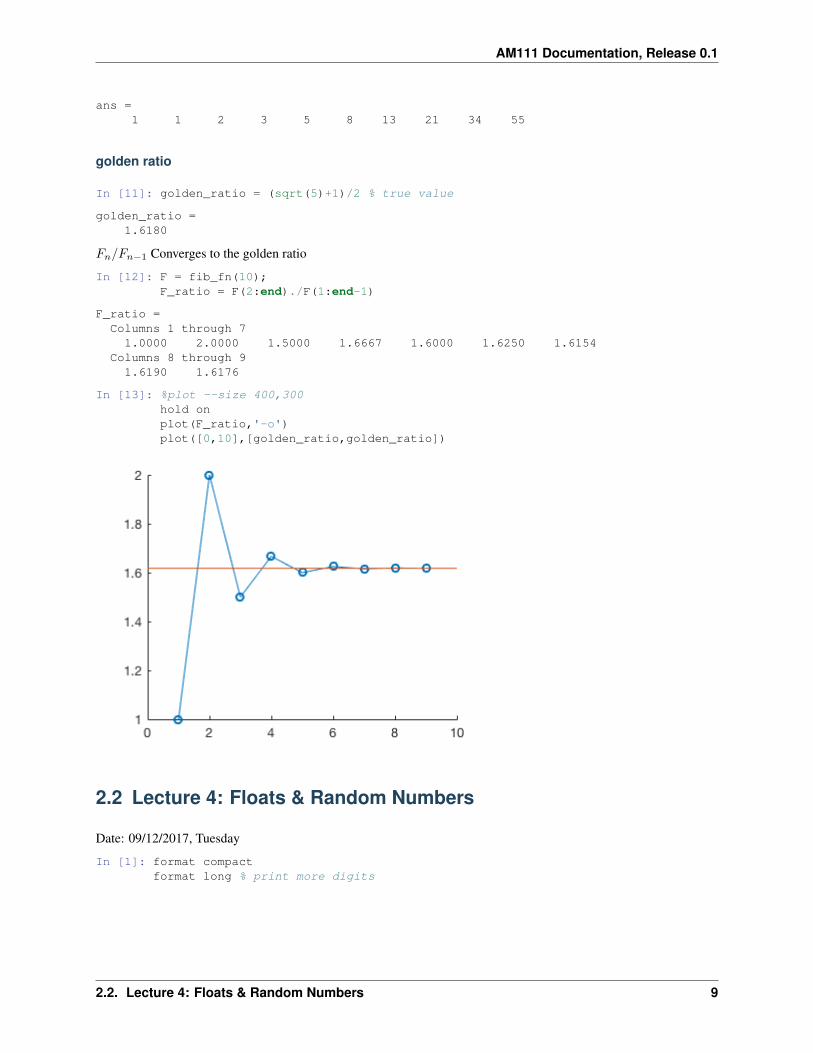
𝐹𝑛/𝐹𝑛−1 Converges to the golden ratio
In [12]: F = fib_fn(10);F_ratio = F(2:end)./F(1:end-1)
F_ratio =Columns 1 through 71.0000 2.0000 1.5000 1.6667 1.6000 1.6250 1.6154
Columns 8 through 91.6190 1.6176
In [13]: %plot --size 400,300hold onplot(F_ratio,'-o')plot([0,10],[golden_ratio,golden_ratio])
2.2 Lecture 4: Floats & Random Numbers
Date: 09/12/2017, Tuesday
In [1]: format compactformat long % print more digits
2.2. Lecture 4: Floats & Random Numbers 9
AM111 Documentation, Release 0.1
2.2.1 Floating point number system
Double precision:
𝑥 = ±(1 + 𝑓)2𝑒
0 ≤ 2𝑡𝑓 < 2𝑡, 𝑡 = 52
−1022 ≤ 𝑒 ≤ 1023
(See lecture slides or textbook for more explantion. This website focuses on codes.)
About parameters
How many binary bits are needed to store 𝑒:
In [2]: log2(2048)
ans =11
Maximum value
Calculate the maximum value of 𝑥 from the formula.
In [3]: t=52;f=(2^t-1)/2^t;(1+f)*2^1023
ans =1.797693134862316e+308
Compare with the built-in function
In [4]: realmax
ans =1.797693134862316e+308
What happens if the value exceeds realmax?
In [5]: 2e308
ans =Inf
Minimum (absolute) value
From the formula
In [6]: 2^-1022
ans =2.225073858507201e-308
Compare with the built-in function
In [7]: realmin
ans =2.225073858507201e-308
MATLAB allows you to go lower than realmin, but no too much.
10 Chapter 2. Lecture & Session Notes
AM111 Documentation, Release 0.1
In [8]: for k=-321:-1:-325fprintf('k = %d, 10^k = %e \n',k,10^k)
end
k = -321, 10ˆk = 9.980126e-322k = -322, 10ˆk = 9.881313e-323k = -323, 10ˆk = 9.881313e-324k = -324, 10ˆk = 0.000000e+00k = -325, 10ˆk = 0.000000e+00
10−323 can be scaled up:
In [9]: 1e-323 * 1e300
ans =9.881312916824931e-24
But 10−324 can’t, as it becomes exactly 0.
In [10]: 1e-324 * 1e300
ans =0
Machine precision
Compute machine precision
From the formula 0 ≤ 2𝑡𝑓 < 2𝑡, 𝑡 = 52
In [11]: 2^(-52)
ans =2.220446049250313e-16
Built-in function:
In [12]: eps
ans =2.220446049250313e-16
Another ways to get eps
In [13]: 1.0-(0.1+0.1+0.1+0.1+0.1+0.1+0.1+0.1+0.1+0.1) % equals to eps/2
ans =1.110223024625157e-16
In [14]: 7/3-4/3-1 % equals to eps
ans =2.220446049250313e-16
Difference between eps and realmin
realmin is about abosolute magnitude, while eps is about relative accuracy. Although a double-precision numbercan represent a value as small as 10−323 (i.e. realmin), the relative error of arithmetic operations can be as large as10−16 (i.e. eps).
Adding 10−16 to 1.0 has no effect at all.
In [15]: 1.0+1e-16-1.0
2.2. Lecture 4: Floats & Random Numbers 11
AM111 Documentation, Release 0.1
ans =0
Adding 10−15 to 1.0 has some effect, although the result is quite inaccurate.
In [16]: 1.0+1e-15-1.0
ans =1.110223024625157e-15
Not a number
In [17]: 0/0
ans =NaN
In [18]: Inf - Inf
ans =NaN
However, Inf can sometimes be meaningful: (MATLAB-only. Not true in low-level languages.)
In [19]: 5/Inf
ans =0
In [20]: 5/0
ans =Inf
2.2.2 Random numbers
Linear congruential generator
In [21]: a = 22695477;c = 1;m = 2^32;N = 2000;
X = zeros(N,1);X(1) = 1000;for j=2:N
X(j)=mod(a*X(j-1)+c,m);end
R = X/m;
Hmm. . . looks pretty random
In [22]: %plot --size 600,200plot(R);
12 Chapter 2. Lecture & Session Notes
AM111 Documentation, Release 0.1
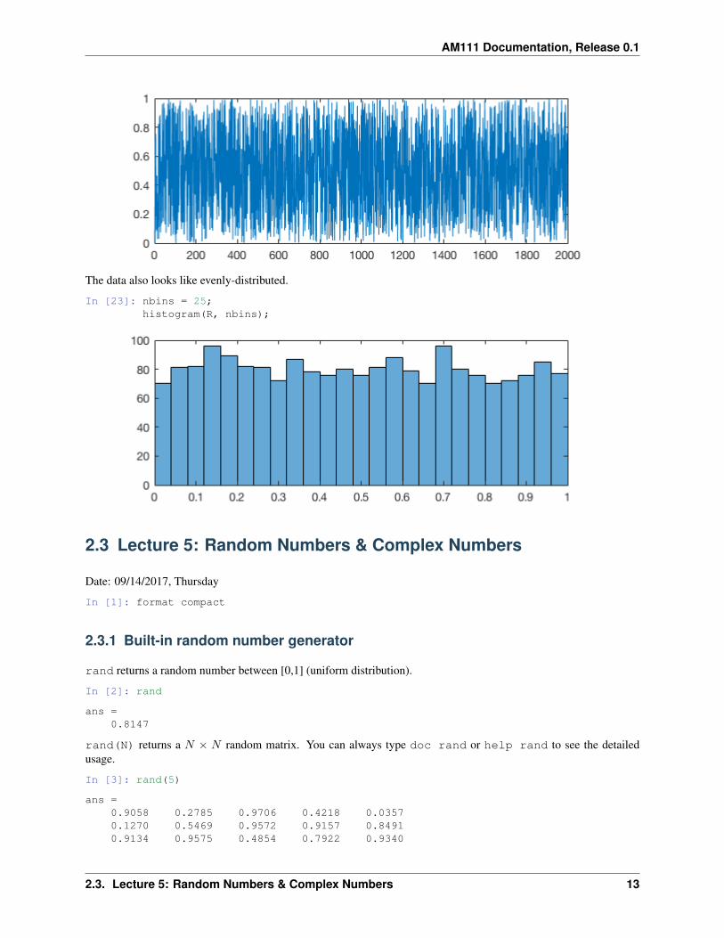
The data also looks like evenly-distributed.
In [23]: nbins = 25;histogram(R, nbins);
2.3 Lecture 5: Random Numbers & Complex Numbers
Date: 09/14/2017, Thursday
In [1]: format compact
2.3.1 Built-in random number generator
rand returns a random number between [0,1] (uniform distribution).
In [2]: rand
ans =0.8147
rand(N) returns a 𝑁 × 𝑁 random matrix. You can always type doc rand or help rand to see the detailedusage.
In [3]: rand(5)
ans =0.9058 0.2785 0.9706 0.4218 0.03570.1270 0.5469 0.9572 0.9157 0.84910.9134 0.9575 0.4854 0.7922 0.9340
2.3. Lecture 5: Random Numbers & Complex Numbers 13
AM111 Documentation, Release 0.1
0.6324 0.9649 0.8003 0.9595 0.67870.0975 0.1576 0.1419 0.6557 0.7577
randi(N) returns an integer between 1 and N.
In [4]: randi(100)
ans =75
randn uses normal distribution, instead of uniform distribution.
In [5]: randn(5)
ans =-0.3034 -1.0689 -0.7549 0.3192 0.62770.2939 -0.8095 1.3703 0.3129 1.0933
-0.7873 -2.9443 -1.7115 -0.8649 1.10930.8884 1.4384 -0.1022 -0.0301 -0.8637
-1.1471 0.3252 -0.2414 -0.1649 0.0774
2.3.2 Complex numbers
Complex number basics
A real number (double-precision) takes 8 Bytes (64 bits). A complex number is a pair of numbers so simply takes 16Bytes (128 bits)
In [6]: x = 3;y = 4;z = x+i*y;
In [7]: whos
Name Size Bytes Class Attributes
ans 5x5 200 doublex 1x1 8 doubley 1x1 8 doublez 1x1 16 double complex
Take conjugate of a complex number:
In [8]: conj(z)
ans =3.0000 - 4.0000i
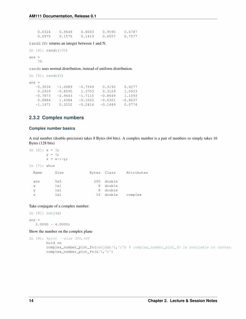
Show the number on the complex plane
In [9]: %plot --size 300,300hold oncomplex_number_plot_fn(conj(z)/5,'r') % complex_number_plot_fn is available on canvas.complex_number_plot_fn(z/5,'b')
14 Chapter 2. Lecture & Session Notes
AM111 Documentation, Release 0.1
3 equivalent ways to compute |𝑧|In [10]: abs(z)
ans =5
In [11]: sqrt(dot(z,z))
ans =5
In [12]: norm(z)
ans =5
The angle of z in degree:
In [13]: angle(z) / pi * 180.0
ans =53.1301
Euler’s Formula
𝑒𝑖𝜃 = cos(𝜃) + 𝑖 sin(𝜃)
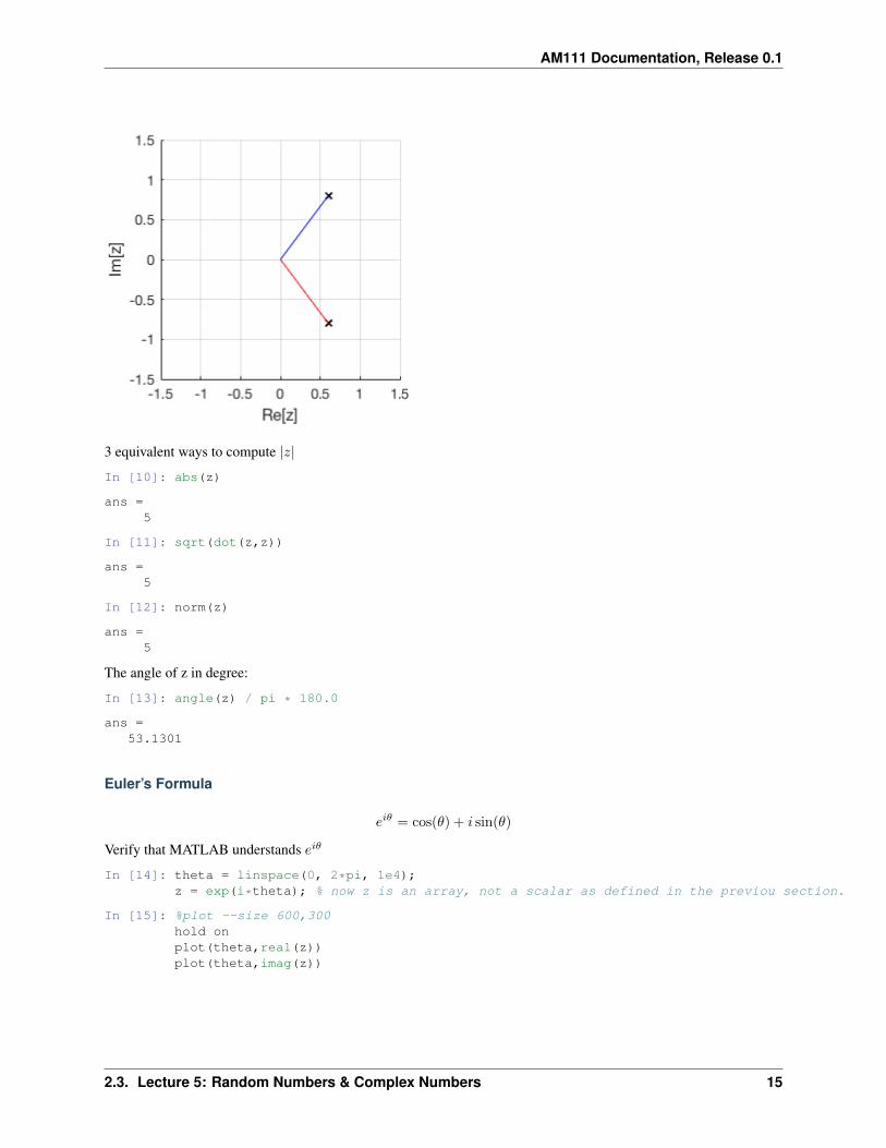
Verify that MATLAB understands 𝑒𝑖𝜃
In [14]: theta = linspace(0, 2*pi, 1e4);z = exp(i*theta); % now z is an array, not a scalar as defined in the previou section.
In [15]: %plot --size 600,300hold onplot(theta,real(z))plot(theta,imag(z))
2.3. Lecture 5: Random Numbers & Complex Numbers 15
AM111 Documentation, Release 0.1
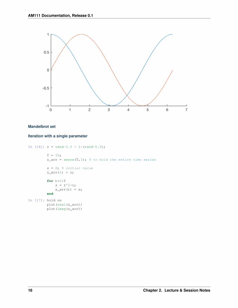
Mandelbrot set
Iteration with a single parameter
In [16]: c = rand-0.5 + i*(rand-0.5);
T = 50;z_arr = zeros(T,1); % to hold the entire time series
z = 0; % initial valuez_arr(1) = z;
for t=2:Tz = z^2+c;z_arr(t) = z;
end
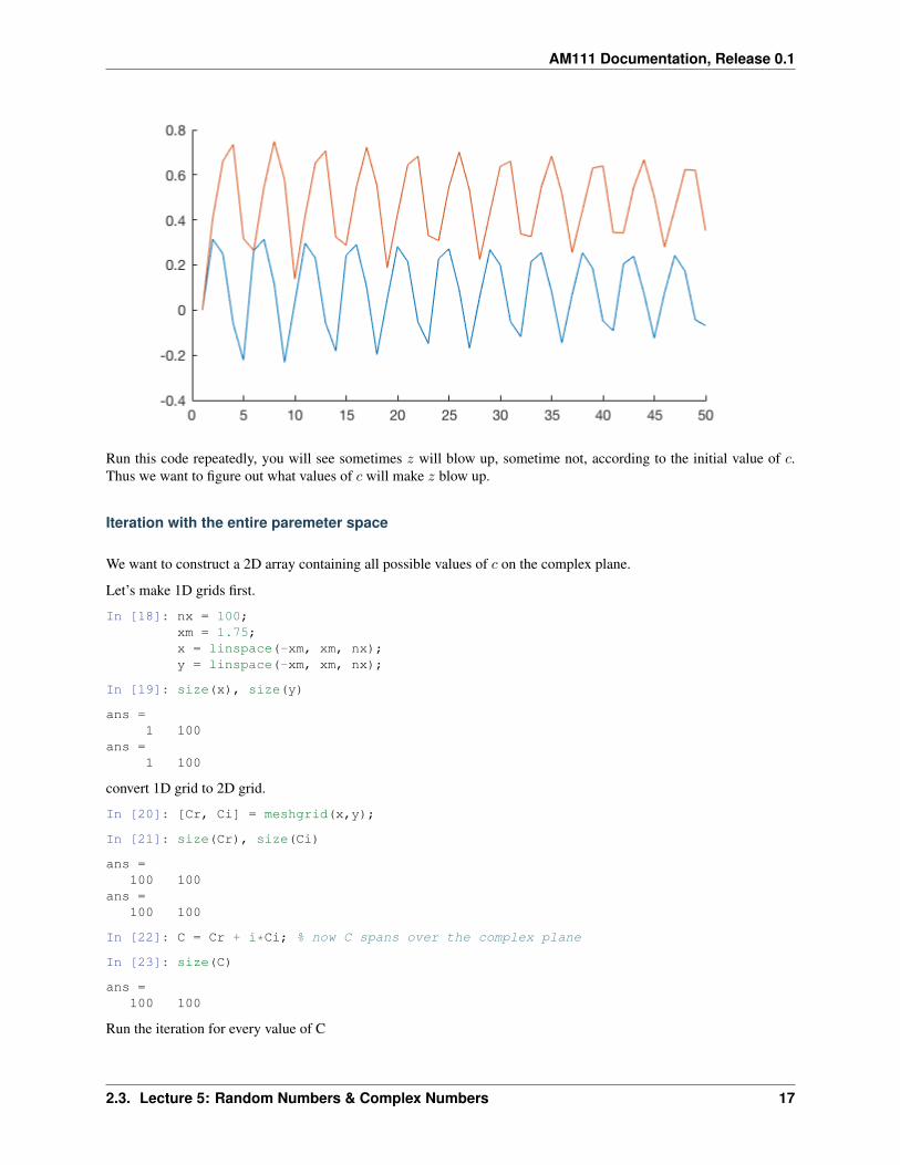
In [17]: hold onplot(real(z_arr))plot(imag(z_arr))
16 Chapter 2. Lecture & Session Notes
AM111 Documentation, Release 0.1
Run this code repeatedly, you will see sometimes 𝑧 will blow up, sometime not, according to the initial value of 𝑐.Thus we want to figure out what values of 𝑐 will make 𝑧 blow up.
Iteration with the entire paremeter space
We want to construct a 2D array containing all possible values of 𝑐 on the complex plane.
Let’s make 1D grids first.
In [18]: nx = 100;xm = 1.75;x = linspace(-xm, xm, nx);y = linspace(-xm, xm, nx);
In [19]: size(x), size(y)
ans =1 100
ans =1 100
convert 1D grid to 2D grid.
In [20]: [Cr, Ci] = meshgrid(x,y);
In [21]: size(Cr), size(Ci)
ans =100 100
ans =100 100
In [22]: C = Cr + i*Ci; % now C spans over the complex plane
In [23]: size(C)
ans =100 100
Run the iteration for every value of C
2.3. Lecture 5: Random Numbers & Complex Numbers 17
AM111 Documentation, Release 0.1
In [24]: T = 50;
Z_final = zeros(nx,nx); % to hold last value of z, at all possible points.
for ix = 1:nxfor iy = 1:nx % we also have nx points in the y-direction
% get the value of c at current point.% note that MATLAB is case-sensitivec = C(ix,iy);
z = 0; % initial value, doesn't matter too muchfor t=2:T
z = z^2+c;endZ_final(ix,iy) = z; % save the last value of z
endend
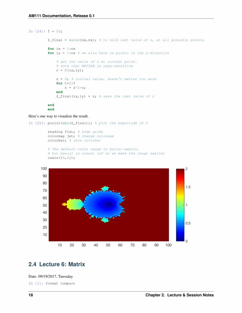
Here’s one way to visualize the result.
In [25]: pcolor(abs(Z_final)); % plot the magnitude of z
shading flat; % hide gridscolormap jet; % change colormapcolorbar; % show colorbar
% The default color range is min(z)~max(z),% but max(z) is almost Inf so we make the range smallercaxis([0,2]);
2.4 Lecture 6: Matrix
Date: 09/19/2017, Tuessday
In [1]: format compact
18 Chapter 2. Lecture & Session Notes

AM111 Documentation, Release 0.1
2.4.1 Matrix operation basics
Making a magic square
In [2]: A = magic(3)
A =8 1 63 5 74 9 2
Take transpose
In [3]: A'
ans =8 3 41 5 96 7 2
Rotate by 90 degree. (Not so useful for linear algebra. Could be useful for image processing.)
In [4]: rot90(A')
ans =4 9 23 5 78 1 6
Sum over each column
In [5]: sum(A)
ans =15 15 15
Another equivalent way
In [6]: sum(A, 1)
ans =15 15 15
Sum over each row
In [7]: sum(A, 2)
ans =151515
Extract the diagonal elements.
In [8]: diag(A)
ans =852
The sum of diagonal elements is also 15, by the definition of a magic square.
In [9]: sum(diag(A))
ans =15
Determinant
2.4. Lecture 6: Matrix 19
AM111 Documentation, Release 0.1
In [10]: det(A)
ans =-360
Matrix inversion 𝐴−1
In [11]: inv(A)
ans =0.1472 -0.1444 0.0639
-0.0611 0.0222 0.1056-0.0194 0.1889 -0.1028
2.4.2 Built-in image for magic square
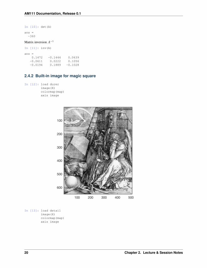
In [12]: load durerimage(X)colormap(map)axis image
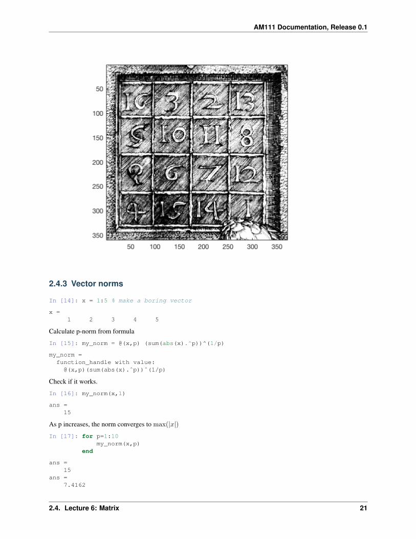
In [13]: load detailimage(X)colormap(map)axis image
20 Chapter 2. Lecture & Session Notes
AM111 Documentation, Release 0.1
2.4.3 Vector norms
In [14]: x = 1:5 % make a boring vector
x =1 2 3 4 5
Calculate p-norm from formula
In [15]: my_norm = @(x,p) (sum(abs(x).^p))^(1/p)
my_norm =function_handle with value:@(x,p)(sum(abs(x).ˆp))ˆ(1/p)
Check if it works.
In [16]: my_norm(x,1)
ans =15
As p increases, the norm converges to max(|𝑥|)In [17]: for p=1:10
my_norm(x,p)end
ans =15
ans =7.4162
2.4. Lecture 6: Matrix 21
AM111 Documentation, Release 0.1
ans =6.0822
ans =5.5937
ans =5.3602
ans =5.2321
ans =5.1557
ans =5.1073
ans =5.0756
ans =5.0541
It blows up at 𝑝 = 442 because 5442 exceeds the realmin.
In [18]: my_norm(x,441), my_norm(x,442)
ans =5
ans =Inf
In [19]: 5^441
ans =1.7611e+308
In [20]: 5^442
ans =Inf
Built-in function norm works for large numbers, though. Think about why.
In [21]: norm(x,441), norm(x,442)
ans =5
ans =5
2.4.4 Conditioning
4x4 magic square
In [22]: B = magic(4)
B =16 2 3 135 11 10 89 7 6 124 14 15 1
It is singular and ill-conditioned.
In [23]: inv(B)
Warning: Matrix is close to singular or badly scaled. Results may be inaccurate. RCOND = 4.625929e-18.ans =
1.0e+15 *
22 Chapter 2. Lecture & Session Notes
AM111 Documentation, Release 0.1
-0.2649 -0.7948 0.7948 0.2649-0.7948 -2.3843 2.3843 0.79480.7948 2.3843 -2.3843 -0.79480.2649 0.7948 -0.7948 -0.2649
In [24]: det(B)
ans =5.1337e-13
In [25]: cond(B)
ans =4.7133e+17
Use 1-norm instead. All norms should have similar order of magnitude.
In [26]: cond(B,1)
Warning: Matrix is close to singular or badly scaled. Results may be inaccurate. RCOND = 4.625929e-18.> In cond (line 46)ans =
2.1617e+17
The condition number reaches 1/eps, leading to large numerical error.
In [27]: 1/eps
ans =4.5036e+15
2.4.5 Sparse matrix
In [28]: A = eye(10)
A =1 0 0 0 0 0 0 0 0 00 1 0 0 0 0 0 0 0 00 0 1 0 0 0 0 0 0 00 0 0 1 0 0 0 0 0 00 0 0 0 1 0 0 0 0 00 0 0 0 0 1 0 0 0 00 0 0 0 0 0 1 0 0 00 0 0 0 0 0 0 1 0 00 0 0 0 0 0 0 0 1 00 0 0 0 0 0 0 0 0 1
Store it in the sparse form saves memory.
In [29]: As = sparse(A)
As =(1,1) 1(2,2) 1(3,3) 1(4,4) 1(5,5) 1(6,6) 1(7,7) 1(8,8) 1(9,9) 1(10,10) 1
2.4. Lecture 6: Matrix 23
AM111 Documentation, Release 0.1
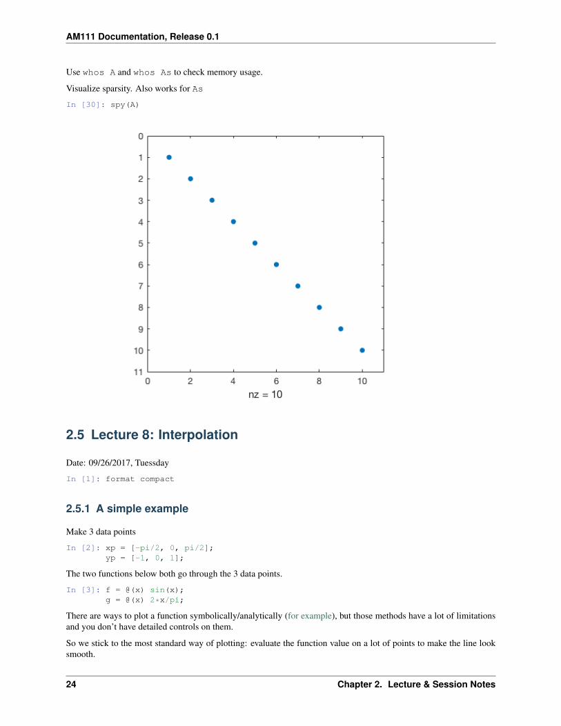
Use whos A and whos As to check memory usage.
Visualize sparsity. Also works for As
In [30]: spy(A)
2.5 Lecture 8: Interpolation
Date: 09/26/2017, Tuessday
In [1]: format compact
2.5.1 A simple example
Make 3 data points
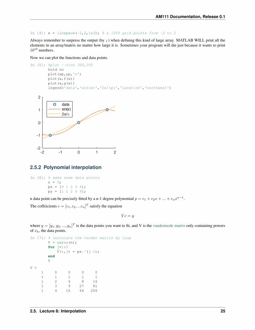
In [2]: xp = [-pi/2, 0, pi/2];yp = [-1, 0, 1];
The two functions below both go through the 3 data points.
In [3]: f = @(x) sin(x);g = @(x) 2*x/pi;
There are ways to plot a function symbolically/analytically (for example), but those methods have a lot of limitationsand you don’t have detailed controls on them.
So we stick to the most standard way of plotting: evaluate the function value on a lot of points to make the line looksmooth.
24 Chapter 2. Lecture & Session Notes
AM111 Documentation, Release 0.1
In [4]: x = linspace(-2,2,1e3); % a 1000 grid points from -2 to 2
Always remember to surpress the output (by ;) when defining this kind of large array. MATLAB WILL print all theelements in an array/matrix no matter how large it is. Sometimes your program will die just because it wants to print1010 numbers.
Now we can plot the functions and data points.
In [5]: %plot --size 300,200hold onplot(xp,yp,'o')plot(x,f(x))plot(x,g(x))legend('data','sin(x)','2x/\pi','Location','northwest')
2.5.2 Polynomial interpolation
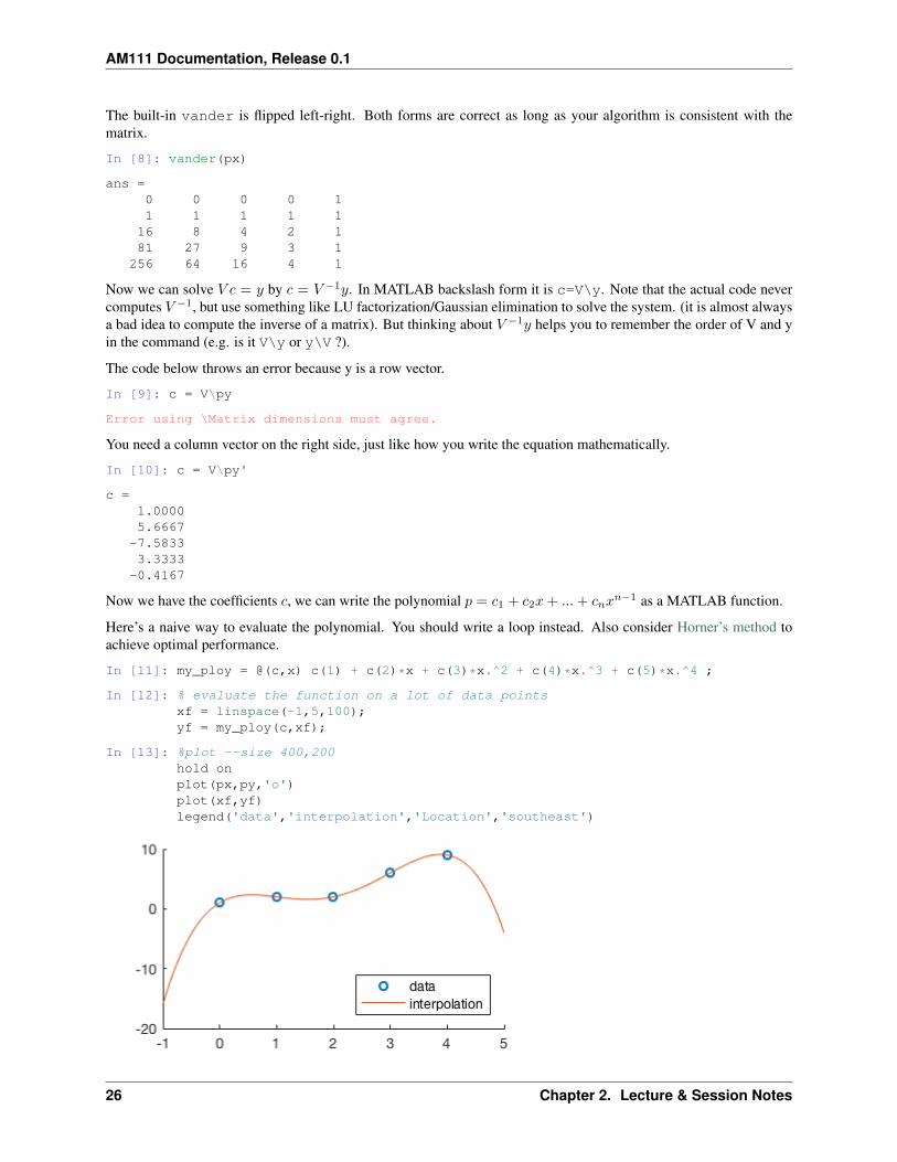
In [6]: % make some data pointsn = 5;px = [0 1 2 3 4];py = [1 2 2 6 9];
n data point can be precisely fitted by a n-1 degree polynomial 𝑝 = 𝑐1 + 𝑐2𝑥 + ... + 𝑐𝑛𝑥𝑛−1.
The coffeicients 𝑐 = [𝑐1, 𝑐2, ...𝑐𝑛]𝑇 satisfy the equation
𝑉 𝑐 = 𝑦
where 𝑦 = [𝑦1, 𝑦2, ..., 𝑦𝑛]𝑇 is the data points you want to fit, and V is the vandermode matrix only containing powersof 𝑥𝑘, the data points.
In [7]: % calculate the vander matrix by loopV = zeros(n);for j=1:5
V(:,j) = px.^(j-1);endV
V =1 0 0 0 01 1 1 1 11 2 4 8 161 3 9 27 811 4 16 64 256
2.5. Lecture 8: Interpolation 25
AM111 Documentation, Release 0.1
The built-in vander is flipped left-right. Both forms are correct as long as your algorithm is consistent with thematrix.
In [8]: vander(px)
ans =0 0 0 0 11 1 1 1 1
16 8 4 2 181 27 9 3 1
256 64 16 4 1
Now we can solve 𝑉 𝑐 = 𝑦 by 𝑐 = 𝑉 −1𝑦. In MATLAB backslash form it is c=V\y. Note that the actual code nevercomputes 𝑉 −1, but use something like LU factorization/Gaussian elimination to solve the system. (it is almost alwaysa bad idea to compute the inverse of a matrix). But thinking about 𝑉 −1𝑦 helps you to remember the order of V and yin the command (e.g. is it V\y or y\V ?).
The code below throws an error because y is a row vector.
In [9]: c = V\py
Error using \Matrix dimensions must agree.
You need a column vector on the right side, just like how you write the equation mathematically.
In [10]: c = V\py'
c =1.00005.6667
-7.58333.3333
-0.4167
Now we have the coefficients 𝑐, we can write the polynomial 𝑝 = 𝑐1 + 𝑐2𝑥 + ... + 𝑐𝑛𝑥𝑛−1 as a MATLAB function.
Here’s a naive way to evaluate the polynomial. You should write a loop instead. Also consider Horner’s method toachieve optimal performance.
In [11]: my_ploy = @(c,x) c(1) + c(2)*x + c(3)*x.^2 + c(4)*x.^3 + c(5)*x.^4 ;
In [12]: % evaluate the function on a lot of data pointsxf = linspace(-1,5,100);yf = my_ploy(c,xf);
In [13]: %plot --size 400,200hold onplot(px,py,'o')plot(xf,yf)legend('data','interpolation','Location','southeast')
26 Chapter 2. Lecture & Session Notes
AM111 Documentation, Release 0.1
2.6 Lecture 11: Odyssey!!!
Date: 10/05/2017, Thursday
You are expected to finish 8+1 tiny tasks. They will help you get prepared for the final project!
Related resources:
• Ryans’s Linux tutorial
• Intro-to-Odssey-S17_am111.pdf on Canvas.
• Odyssey quickstart guide
• MATLAB on Odyssey
• Parallel MATLAB on Odyssey
2.6.1 Task 1: Command line on your laptop
Preparation
Read Session 4 note, especially Ryans’s tutorial if you didn’t come to Monday’s session.
After reading Chapter 1 to Chapter 5, you should at least know the following Linux commands
• ls
• pwd
• mkdir
• cd
• mv
• rm and rm -rf
• cp and cp -r
If you choose vi/vim as your text editor, read Chapter 6. Then you should at least know the following vim commands
• i
• esc
• :wq
• :q!
Find your own tutorial if you choose other text editors.
Writing code in terminal
Task: Use vim or other command line text editer to create a matlab file hello.m with the content “disp(‘hello world!’)”
We use vim as an example.
First, create a text file by
vim hello.m
2.6. Lecture 11: Odyssey!!! 27

AM111 Documentation, Release 0.1
(If hello.m already exists, then it will just open that file)
Inside vim, type i to enter the Insert Mode.
Then type the code as usual. For example
disp('hello world!')
After writting the content, type esc to go back to Command Mode.
Finally, type :wq to save and quit vim.
Again, read Chapter 6 for more vim usages!
Tips: You can check the content of hello.m by a graphic editer. On Mac, you can use open ./ to open the graphicfinder, and then open hello.m that you’ve just created. On Odyssey (See Task 2), there’s no graphic editor, so you willalso use vim to check the file content.
Running MATLAB interactively in terminal
Windows users can jump to Task 2 because I am not sure if the following stuff would work.
Find the MATLAB executable path on your laptop. On Mac it should be something like
/Applications/MATLAB_R2017a.app/bin/matlab
Running the above command will open the traditional graphic version of MATLAB.
To only use the command line, add 3 options:
/Applications/MATLAB_R2017a.app/bin/matlab -nojvm -nosplash -nodesktop
Play with this command line version of MATLAB for a while. Type exit to quit.
Set shortcut
If you are tired with typing this long command, you can set
alias matlab='/Applications/MATLAB_R2017a.app/bin/matlab'
Then you can simply type matlab to launch the program. However, this shortcut will go away if you close theterminal. To make it a permanent configuration, add the above command to a system file called ~/.bash_profile. Youcan edit it by vim for example:
vim ~/.bash_profile
Running MATLAB scripts in terminal
cd to the directory where you saved the hello.m file. You can execute it by
matlab -nojvm -nosplash -nodesktophello
Or you can use ‘-r’ to combine two commands together
matlab -nojvm -nosplash -nodesktop -r hello
28 Chapter 2. Lecture & Session Notes
AM111 Documentation, Release 0.1
If you didn’t set shortcut, the full command would be
/Applications/MATLAB_R2017a.app/bin/matlab -nojvm -nosplash -nodesktop -r hello
(I actually prefer this command line version to the complicated graphic version!)
2.6.2 Task 2: Command line on Odyssey
Login
Login to Odyssey by
Check Odyssey website if you have any trouble.
Tips: You can open multiple terminals and login to Odyssey, if one is not enough for you.
Basic navigation
Repeat the basic Linux commands, but this time on Odyssey, not on your laptop.
You should see Mac and Linux (Odyssey) commands are almost identical.
File transfer
Use scp
You can transfer files by the built-in scp (security-copy) command. Make sure you are running this command onyour laptop, not on odyssey.
From you laptop to Odyssey (first figure out your Odyssey home directory path by pwd)
scp local_file_path [email protected]:/path_shown_by_pwd_on_Odyssey
Try to transfer *hello.m* that you wrote in Task 1 to Odyssey! You will be asked to enter your password again.
From to Odyssey to your laptop is just reversing the arguments
scp [email protected]:/file_path_on_odyssey local_file_path
Use scp -r for transfering directory (similar to cp -r)
Use other tools
Use Filezilla if you need to transfer a lot of file!
2.6.3 Task 3: MATLAB on Odyssey
Load MATLAB
Load MATLAB by
2.6. Lecture 11: Odyssey!!! 29
AM111 Documentation, Release 0.1
module load matlab
(If you get an error, run source new-modules.sh and try again.)
It loads the lastest version by default. You can check the version by which
[username]$ which matlabalias matlab='matlab -singleCompThread'/n/sw/matlab-R2017a/bin/matlab
Or you can load a specific version
module load matlab/R2017a-fasrc01
Use this RC portal to find avaiable software and the corresponding loading command. Search for MATLAB. Howmany different verions do you see?
Run MATLAB
After loading MATLAB, you can run it by: (same as on your laptop)
matlab -nojvm -nosplash -nodesktop
The 3 options are crucial because there’s no graphical user interface on Odyssey.
Play with it, and type exit to quit.
Run hello.m by matlab -nojvm -nosplash -nodesktop -r hello.
2.6.4 Task 4: Interactive Job on Odyssey
After logging into Odyssey, you are on a home node with very few computational resources. For any serious computingwork you need to switch to a compute node. The easiest way is to do this interactively (more about interative mode):
srun -t 0-0:30 -c 4 -N 1 --pty -p interact /bin/bash
Here we request 30 minutes of computing time (-t 0-0:30) on 4 CPUs (-c 4), on a single computer (-N 1),using interactive mode (--pty and /bin/bash).
Warning: Don’t request too many CPUs! This will make you wait for much longer.
-p interact only means you are requesting CPUs on the interactive partition, but doesn’t mean that you want itto run interactively. The following command starts interactive mode on the general partition (more about partition).
srun -t 0-0:30 -c 4 -N 1 --pty -p general /bin/bash
Then repeat what you’ve done in Task 3.
2.6.5 Task 5: Batch Job on Odyssey
If your job runs for hours or even days, you can submit it as a batch job, so you don’t need to keep your terminal openall the time. You are allowed to log out and go away while the job is runnning.
Create a file called runscript.sh with the following content. (you can use vim to create such a text file)
30 Chapter 2. Lecture & Session Notes

AM111 Documentation, Release 0.1
#!/bin/bash#SBATCH -J Matlabjob1#SBATCH -p general#SBATCH -c 1 # single CPU#SBATCH -t 00:05:00#SBATCH --mem=400M # memory#SBATCH -o %j.o # output filename#SBATCH -e %j.e # error filename
## LOAD SOFTWARE ENV ##source new-modules.shmodule purgemodule load matlab/R2017a-fasrc01
## EXECUTE CODE ##matlab -nojvm -nodisplay -nosplash -r hello
It just puts the options you’ve used in Task 4 into a text file.
Make sure runscript.sh is at the same directory as hello.m, then execute
sbatch runscript.sh
Use sacct to check job status. You should get some output files once it is finished. (more about submitting andmonitoring jobs)
Tips: always test your code in interactive mode before submitting a batch job!
2.6.6 Task 6: Use MATLAB-parallel on your laptop
Make sure you’ve installed the parallel toolbox. To start the command line version, remove the -nojvm option whenusing parallel mode. (The original graphic version works as usual)
matlab -nosplash -nodesktop
Initialize parallel mode by
In [1]: parpool('local', 2)
Starting parallel pool (parpool) using the 'local' profile ...connected to 2 workers.
ans =
Pool with properties:
Connected: trueNumWorkers: 2
Cluster: localAttachedFiles: IdleTimeout: 30 minutes (30 minutes remaining)SpmdEnabled: true
Then run this script for several times to make sure you get speed-up by using parallel for-loop (parfor)
In [4]: n = 1e9;
X = 0;
2.6. Lecture 11: Odyssey!!! 31
AM111 Documentation, Release 0.1
ticfor i = 1:n
X = X + 1;endT = toc;fprintf('serial time: %f; result: %d \n',T,X)
X = 0;ticparfor i = 1:n
X = X + 1;endT = toc;fprintf('parallel time: %f; result: %d \n',T,X)
serial time: 2.724932; result: 1000000000parallel time: 1.748450; result: 1000000000
Tips: For command line version of MATLAB, save the code as parallel_timing.m, and then executeparallel_timing inside MATLAB.
Finally, quit the parallel mode
In [5]: delete(gcp)
2.6.7 Task 7: Use MATLAB-parallel on Odyssey interactive mode
Repeat what you’ve done in Task 6, but on Odyssey. This might not be as straightforward as you expected!
You need to request enough memory for the parallel tool box
srun -t 0-0:30 -c 4 -N 1 --mem-per-cpu 4000 --pty -p interact /bin/bash
Environment variable SLURM_CPUS_PER_TASK tells you how many CPUs are available
echo $SLURM_CPUS_PER_TASK4
For parallel support, you need to call matlab-default instead of matlab to launch the program, as describedhere.
module load matlabmatlab-default -nosplash -nodesktop
Inside MATLAB, you can again check the number of CPUs by
getenv('SLURM_CPUS_PER_TASK')ans = '4'
Initialize parallel mode by (this is a general code for any number of CPUs)
parpool('local', str2num(getenv('SLURM_CPUS_PER_TASK')) )
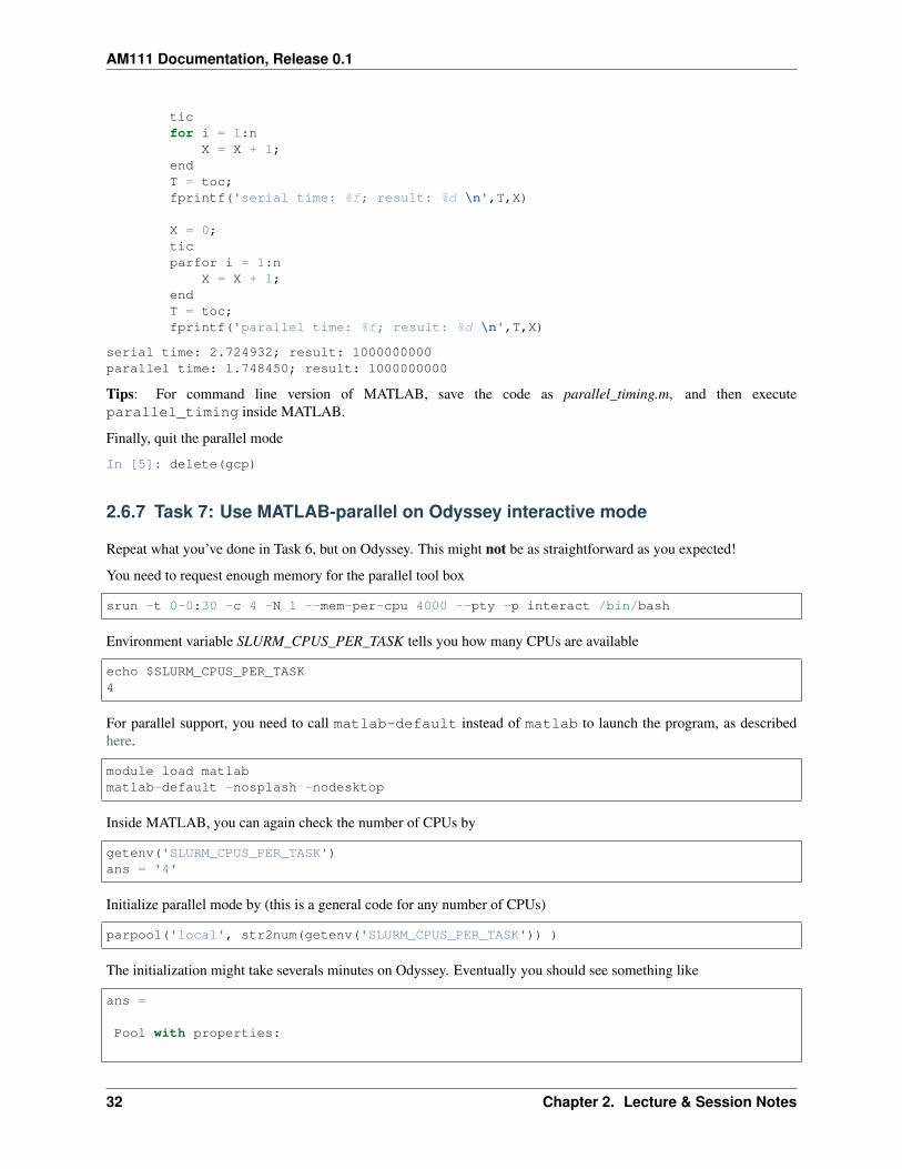
The initialization might take severals minutes on Odyssey. Eventually you should see something like
ans =
Pool with properties:
32 Chapter 2. Lecture & Session Notes
AM111 Documentation, Release 0.1
Connected: trueNumWorkers: 4
Cluster: localAttachedFiles: IdleTimeout: 30 minutes (30 minutes remaining)SpmdEnabled: true
Then, execute the parallel_timing.m script in Task 6. You should see a speed-up like that
>> parallel_timingserial time: 12.228084; result: 1000000000parallel time: 2.667366; result: 1000000000
2.6.8 Task 8: MATLAB-parallel as batch Job
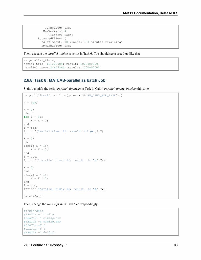
Sightly modify the script parallel_timing.m in Task 6. Call it parallel_timing_batch.m this time.
parpool('local', str2num(getenv('SLURM_CPUS_PER_TASK')))
n = 1e9;
X = 0;ticfor i = 1:n
X = X + 1;endT = toc;fprintf('serial time: %f; result: %d \n',T,X)
X = 0;ticparfor i = 1:n
X = X + 1;endT = toc;fprintf('parallel time: %f; result: %d \n',T,X)
X = 0;ticparfor i = 1:n
X = X + 1;endT = toc;fprintf('parallel time: %f; result: %d \n',T,X)
delete(gcp)
Then, change the runscript.sh in Task 5 correspondingly
#!/bin/bash#SBATCH -J timing#SBATCH -o timing.out#SBATCH -e timing.err#SBATCH -N 1#SBATCH -c 4#SBATCH -t 0-00:20
2.6. Lecture 11: Odyssey!!! 33
AM111 Documentation, Release 0.1
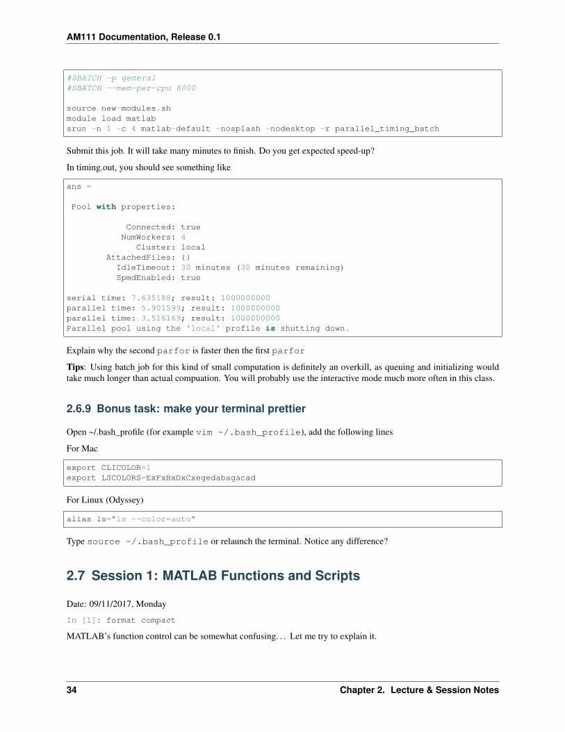
#SBATCH -p general#SBATCH --mem-per-cpu 8000
source new-modules.shmodule load matlabsrun -n 1 -c 4 matlab-default -nosplash -nodesktop -r parallel_timing_batch
Submit this job. It will take many minutes to finish. Do you get expected speed-up?
In timing.out, you should see something like
ans =
Pool with properties:
Connected: trueNumWorkers: 4
Cluster: localAttachedFiles: IdleTimeout: 30 minutes (30 minutes remaining)SpmdEnabled: true
serial time: 7.635188; result: 1000000000parallel time: 5.901599; result: 1000000000parallel time: 3.516169; result: 1000000000Parallel pool using the 'local' profile is shutting down.
Explain why the second parfor is faster then the first parfor
Tips: Using batch job for this kind of small computation is definitely an overkill, as queuing and initializing wouldtake much longer than actual compuation. You will probably use the interactive mode much more often in this class.
2.6.9 Bonus task: make your terminal prettier
Open ~/.bash_profile (for example vim ~/.bash_profile), add the following lines
For Mac
export CLICOLOR=1export LSCOLORS=ExFxBxDxCxegedabagacad
For Linux (Odyssey)
alias ls="ls --color=auto"
Type source ~/.bash_profile or relaunch the terminal. Notice any difference?
2.7 Session 1: MATLAB Functions and Scripts
Date: 09/11/2017, Monday
In [1]: format compact
MATLAB’s function control can be somewhat confusing. . . Let me try to explain it.
34 Chapter 2. Lecture & Session Notes

AM111 Documentation, Release 0.1
2.7.1 3 ways to execute MATLAB codes
You can run MATLAB codes in these ways:
• Executing codes directly in the interactive console
• Put codes in a script (an m-file), and execute the script in the console
• Put codes in a function (also an m-file), and execute the function in the console
Executing codes directly
You know how to run the codes in the interactive console:
In [2]: a=1;b=2;2*a+5*b
ans =12
To avoid re-typing the formula 2*a+5*b over and over again, you can create an inline function in the interativeenvironment.
In [3]: f = @(a,b) 2*a+5*b
f =function_handle with value:@(a,b)2*a+5*b
In [4]: f(1,2)f(2,3)
ans =12
ans =19
Writing a script
A script simply allows you to execute many lines of codes at once. It is not a function. There’s no input and outputvariables.
To open a new script, type “edit” in the console or click on the “New” Button.
In [5]: edit
Save the following code into a file with the suffix “.m”
In [6]: %%file my_script.ma=1;b=2;2*a+5*b
Created file '/Users/zhuangjw/Research/Computing/personal_web/AM111/docs/my_script.m'.
Execute the script by typing its file name in the console. Make sure your working directory is the same as the script’sdirectory.
In [7]: my_script
ans =12
2.7. Session 1: MATLAB Functions and Scripts 35
AM111 Documentation, Release 0.1
You can definitely change parameters a, b in your script and re-run the script over and over again. However, to havea better control on input arguments, you need to write a function, a not script.
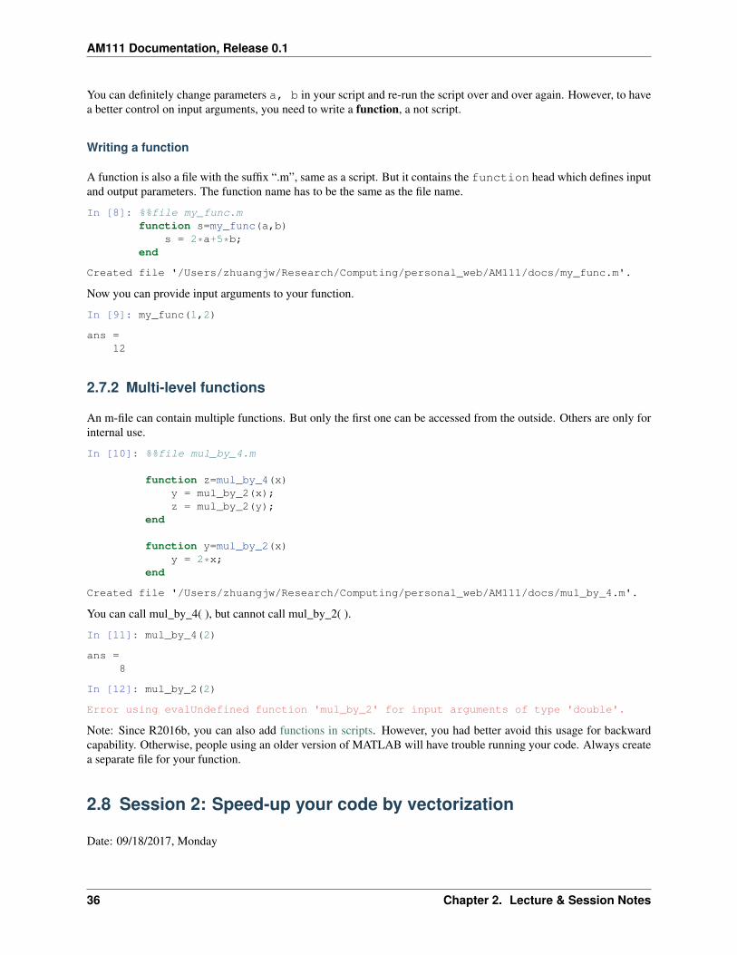
Writing a function
A function is also a file with the suffix “.m”, same as a script. But it contains the function head which defines inputand output parameters. The function name has to be the same as the file name.
In [8]: %%file my_func.mfunction s=my_func(a,b)
s = 2*a+5*b;end
Created file '/Users/zhuangjw/Research/Computing/personal_web/AM111/docs/my_func.m'.
Now you can provide input arguments to your function.
In [9]: my_func(1,2)
ans =12
2.7.2 Multi-level functions
An m-file can contain multiple functions. But only the first one can be accessed from the outside. Others are only forinternal use.
In [10]: %%file mul_by_4.m
function z=mul_by_4(x)y = mul_by_2(x);z = mul_by_2(y);
end
function y=mul_by_2(x)y = 2*x;
end
Created file '/Users/zhuangjw/Research/Computing/personal_web/AM111/docs/mul_by_4.m'.
You can call mul_by_4( ), but cannot call mul_by_2( ).
In [11]: mul_by_4(2)
ans =8
In [12]: mul_by_2(2)
Error using evalUndefined function 'mul_by_2' for input arguments of type 'double'.
Note: Since R2016b, you can also add functions in scripts. However, you had better avoid this usage for backwardcapability. Otherwise, people using an older version of MATLAB will have trouble running your code. Always createa separate file for your function.
2.8 Session 2: Speed-up your code by vectorization
Date: 09/18/2017, Monday
36 Chapter 2. Lecture & Session Notes
AM111 Documentation, Release 0.1
This session is mostly about reviewing Lecture 4 and 5. This page just introduces an additional trick to make yourcode faster and cleaner.
2.8.1 For loops
You already know how to create a Mandelbrot set by writting tons of “for” loops. If not, see Lecture 5’s note.
In [1]: %%file mande_by_loops.mfunction Z_final = mande_by_loops(C, T)
[nx,ny] = size(C);Z_final = zeros(nx,ny); % to hold last value of z, at all possible points.
for ix = 1:nxfor iy = 1:ny
% get the value of c at current point.% note that MATLAB is case-sensitivec = C(ix,iy);z = 0; % initial value, doesn't matter too muchfor t=2:T
z = z^2+c;endZ_final(ix,iy) = z; % save the last value of z
endend
end
Created file '/Users/zhuangjw/Research/Computing/personal_web/AM111/docs/mande_by_loops.m'.
2.8.2 Vectorization
The above function has 3 “for” loops, but 2 of them are not necessary, because you can operate on the entire array.
In [2]: %%file mande_by_vec.mfunction Z = mande_by_vec(C, T)
% vectorized over C and Z
[nx,ny] = size(C);Z = zeros(nx,ny);for t=2:T
Z = Z.^2+C;end
end
Created file '/Users/zhuangjw/Research/Computing/personal_web/AM111/docs/mande_by_vec.m'.
2.8.3 Performance comparision
Compared to the for-loop version, this vectorized version is much shorter, and 20x faster!
In [3]: % initializationnx = 1000;xm = 1.75;
2.8. Session 2: Speed-up your code by vectorization 37
AM111 Documentation, Release 0.1
x = linspace(-xm, xm, nx);y = linspace(-xm, xm, nx);[Cr, Ci] = meshgrid(x,y);C = Cr + i*Ci;
T = 50;
% use loopsticZ_loop = mande_by_loops(C,T);toc
% use vectorizationticZ_vec = mande_by_vec(C,T);toc
% check if results are equalisequal(Z_vec,Z_loop)
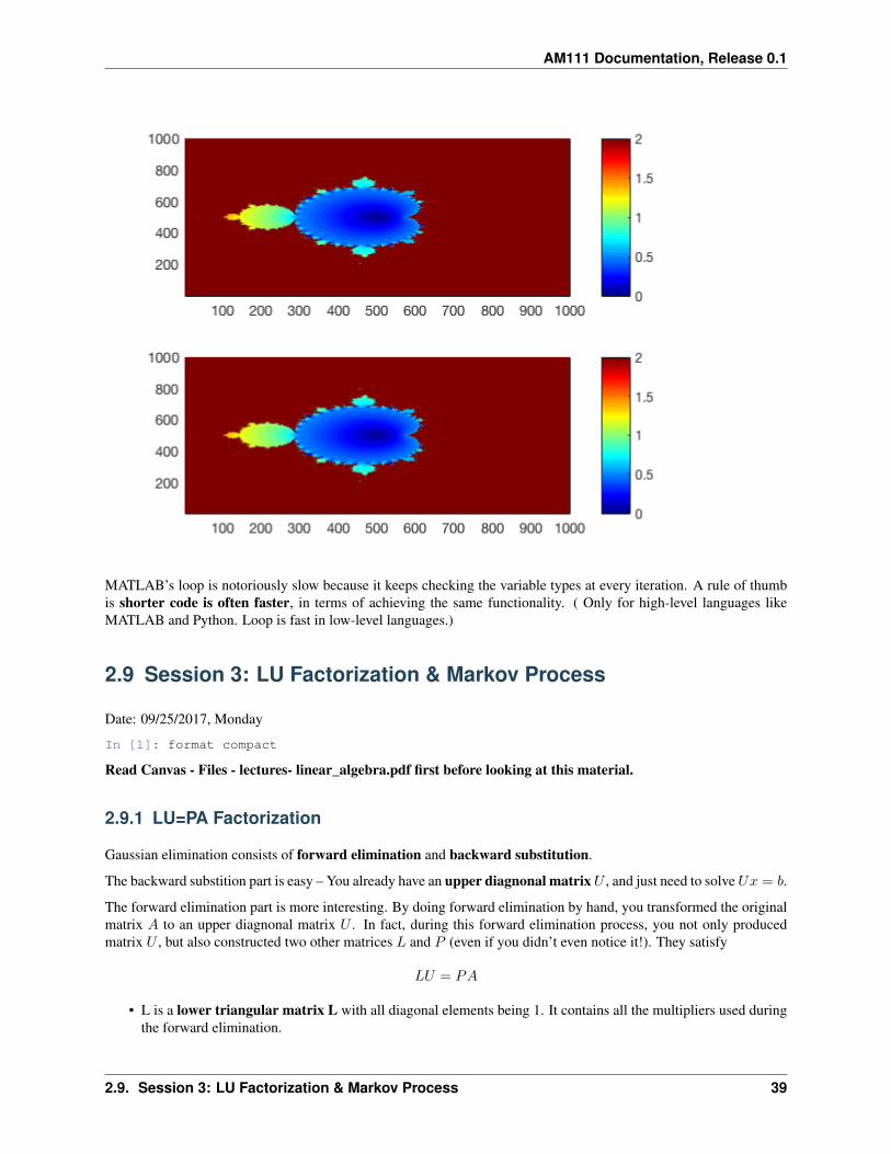
% plot two resultssubplot(211);pcolor(abs(Z_loop));shading flat;colormap jet; colorbar;caxis([0,2]);
subplot(212);pcolor(abs(Z_vec));shading flat;colormap jet; colorbar;caxis([0,2]);
Elapsed time is 4.883975 seconds.Elapsed time is 0.255324 seconds.
ans =
logical
1
38 Chapter 2. Lecture & Session Notes
AM111 Documentation, Release 0.1
MATLAB’s loop is notoriously slow because it keeps checking the variable types at every iteration. A rule of thumbis shorter code is often faster, in terms of achieving the same functionality. ( Only for high-level languages likeMATLAB and Python. Loop is fast in low-level languages.)
2.9 Session 3: LU Factorization & Markov Process
Date: 09/25/2017, Monday
In [1]: format compact
Read Canvas - Files - lectures- linear_algebra.pdf first before looking at this material.
2.9.1 LU=PA Factorization
Gaussian elimination consists of forward elimination and backward substitution.
The backward substition part is easy – You already have an upper diagnonal matrix 𝑈 , and just need to solve 𝑈𝑥 = 𝑏.
The forward elimination part is more interesting. By doing forward elimination by hand, you transformed the originalmatrix 𝐴 to an upper diagnonal matrix 𝑈 . In fact, during this forward elimination process, you not only producedmatrix 𝑈 , but also constructed two other matrices 𝐿 and 𝑃 (even if you didn’t even notice it!). They satisfy
𝐿𝑈 = 𝑃𝐴
• L is a lower triangular matrix L with all diagonal elements being 1. It contains all the multipliers used duringthe forward elimination.
2.9. Session 3: LU Factorization & Markov Process 39

AM111 Documentation, Release 0.1
• 𝑃 is a permutation matrix containing only 0 and 1. It accounts for all row-swapings during the forwardelimination.
Row operation as matrix multiplication
Basic idea
To understand how 𝐿𝑈 = 𝑃𝐴 works, you should always keep in mind that
row operation = left multiply
Or more verbosely
A row operation on matrix A = left-multiply a matrix L to A (i.e. calculate LA)
This is a crucial concept in linear algebra.
Let’s see an example:
In [2]: A = [10 -7 0; -3 2 6 ;5 -1 5]
A =10 -7 0-3 2 65 -1 5
Perform the first step of gaussian elimination, i.e. add 0.3*row1 to row2.
In [3]: A1 = A; % make a copyA1(2,:) = A(2,:)+0.3*A(1,:)
A1 =10.0000 -7.0000 0
0 -0.1000 6.00005.0000 -1.0000 5.0000
There’s another way to perform the above row-operation: left-multiply A by an elementary matrix.
In [4]: L1 = [1,0,0; 0.3,1,0; 0,0,1] % make our elementary matrix
L1 =1.0000 0 00.3000 1.0000 0
0 0 1.0000
In [5]: L1*A
ans =10.0000 -7.0000 0
0 -0.1000 6.00005.0000 -1.0000 5.0000
L1*A gives the same result as the previous row-operation!
Let’s repeat this idea again:
row operation = left multiply
40 Chapter 2. Lecture & Session Notes
AM111 Documentation, Release 0.1
Find elementary matrix
How to find out the matrix L1? Just perform the row-operation to an identity matrix
In [6]: L1 = eye(3); % 3x3 identity matrixL1(2,:) = L1(2,:)+0.3*L1(1,:) % the row-operation you want to "encode" into this matrix
L1 =1.0000 0 00.3000 1.0000 0
0 0 1.0000
Then you can perform L1*A to apply this row-operation on any matrix A.
Same for the permutation operation, as it is also an elementary row operation.
In [7]: Ap = A; % make a copy% swap raw 1 and 2Ap(2,:) = A(1,:);Ap(1,:) = A(2,:);Ap
Ap =-3 2 610 -7 05 -1 5
You can “encode” this row-swapping operation into an elementary permutation matrix.
In [8]: I = eye(3); % 3x3 identity matrixP1 = I;
% swap raw 1 and 2P1(2,:) = I(1,:);P1(1,:) = I(2,:);P1
P1 =0 1 01 0 00 0 1
Multiplying A by P1 is equivalent to permuting A directly:
In [9]: P1*A % same as Ap
ans =-3 2 610 -7 05 -1 5
Get L during forward elimination
For simplicity, assume you don’t need permutation steps. Then you just transform an arbrary 3x3 matrix A (non-singular, of course) to an upper-diagnoal matrix U by 3 row operations. Such operations are equivalent to multiplyingA by 3 matrices 𝐿1, 𝐿2, 𝐿3
𝐴 → 𝐿1𝐴 → 𝐿2𝐿1𝐴 → 𝐿3𝐿2𝐿1𝐴 = 𝑈
We can rewrite it as
𝐴 = (𝐿3𝐿2𝐿1)−1𝑈
2.9. Session 3: LU Factorization & Markov Process 41
AM111 Documentation, Release 0.1
Or
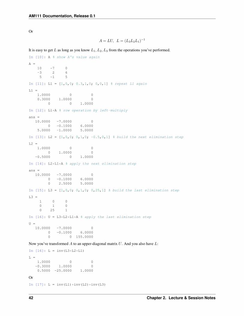
𝐴 = 𝐿𝑈, 𝐿 = (𝐿3𝐿2𝐿1)−1
It is easy to get 𝐿 as long as you know 𝐿1, 𝐿2, 𝐿3 from the operations you’ve performed.
In [10]: A % show A's value again
A =10 -7 0-3 2 65 -1 5
In [11]: L1 = [1,0,0; 0.3,1,0; 0,0,1] % repeat L1 again
L1 =1.0000 0 00.3000 1.0000 0
0 0 1.0000
In [12]: L1*A % row operation by left-multiply
ans =10.0000 -7.0000 0
0 -0.1000 6.00005.0000 -1.0000 5.0000
In [13]: L2 = [1,0,0; 0,1,0; -0.5,0,1] % build the next elimination step
L2 =1.0000 0 0
0 1.0000 0-0.5000 0 1.0000
In [14]: L2*L1*A % apply the next elimination step
ans =10.0000 -7.0000 0
0 -0.1000 6.00000 2.5000 5.0000
In [15]: L3 = [1,0,0; 0,1,0; 0,25,1] % build the last elimination step
L3 =1 0 00 1 00 25 1
In [16]: U = L3*L2*L1*A % apply the last elimination step
U =10.0000 -7.0000 0
0 -0.1000 6.00000 0 155.0000
Now you’ve transformed 𝐴 to an upper-diagonal matrix 𝑈 . And you also have 𝐿:
In [16]: L = inv(L3*L2*L1)
L =1.0000 0 0
-0.3000 1.0000 00.5000 -25.0000 1.0000
Or
In [17]: L = inv(L1)*inv(L2)*inv(L3)
42 Chapter 2. Lecture & Session Notes
AM111 Documentation, Release 0.1
L =1.0000 0 0
-0.3000 1.0000 00.5000 -25.0000 1.0000
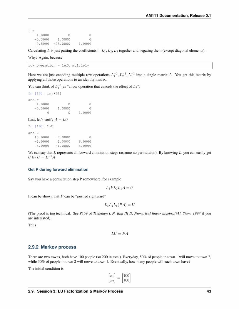
Calculating 𝐿 is just putting the coefficients in 𝐿1, 𝐿2, 𝐿3 together and negating them (except diagonal elements).
Why? Again, because
row operation = left multiply
Here we are just encoding multiple row operations 𝐿−11 , 𝐿−1
2 , 𝐿−13 into a single matrix 𝐿. You get this matrix by
applying all those operations to an identity matrix.
You can think of 𝐿−11 as “a row operation that cancels the effect of 𝐿1“:
In [18]: inv(L1)
ans =1.0000 0 0
-0.3000 1.0000 00 0 1.0000
Last, let’s verify 𝐴 = 𝐿𝑈
In [19]: L*U
ans =10.0000 -7.0000 0-3.0000 2.0000 6.00005.0000 -1.0000 5.0000
We can say that 𝐿 represents all forward elimination steps (assume no permutaion). By knowing 𝐿, you can easily get𝑈 by 𝑈 = 𝐿−1𝐴
Get P during forward elimination
Say you have a permutation step P somewhere, for example
𝐿3𝑃𝐿2𝐿1𝐴 = 𝑈
It can be shown that 𝑃 can be “pushed rightward”
𝐿3𝐿2𝐿1(𝑃𝐴) = 𝑈
(The proof is too technical. See P159 of Trefethen L N, Bau III D. Numerical linear algebra[M]. Siam, 1997 if youare interested).
Thus
𝐿𝑈 = 𝑃𝐴
2.9.2 Markov process
There are two towns, both have 100 people (so 200 in total). Everyday, 50% of people in town 1 will move to town 2,while 30% of people in town 2 will move to town 1. Eventually, how many people will each town have?
The initial condition is [𝑥1
𝑥2
]=
[100100
]
2.9. Session 3: LU Factorization & Markov Process 43
AM111 Documentation, Release 0.1
Each day [𝑥1
𝑥2
]→
[𝑥1 − 0.5𝑥1 + 0.3𝑥2
𝑥2 + 0.5𝑥1 − 0.3𝑥2
]=
[0.5𝑥1 + 0.3𝑥2
0.5𝑥1 + 0.7𝑥2
]=
[0.5 0.30.5 0.7
] [𝑥1
𝑥2
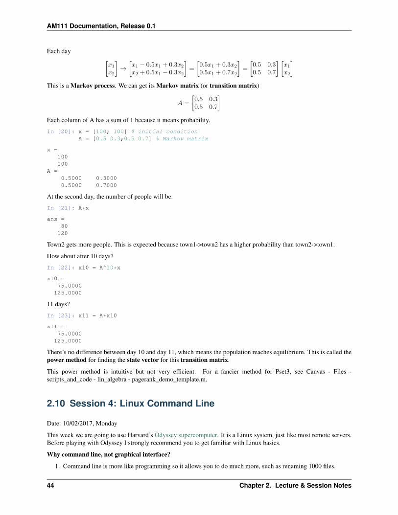
]This is a Markov process. We can get its Markov matrix (or transition matrix)
𝐴 =
[0.5 0.30.5 0.7
]Each column of A has a sum of 1 because it means probability.
In [20]: x = [100; 100] % initial conditionA = [0.5 0.3;0.5 0.7] % Markov matrix
x =100100
A =0.5000 0.30000.5000 0.7000
At the second day, the number of people will be:
In [21]: A*x
ans =80
120
Town2 gets more people. This is expected because town1->town2 has a higher probability than town2->town1.
How about after 10 days?
In [22]: x10 = A^10*x
x10 =75.0000125.0000
11 days?
In [23]: x11 = A*x10
x11 =75.0000125.0000
There’s no difference between day 10 and day 11, which means the population reaches equilibrium. This is called thepower method for finding the state vector for this transition matrix.
This power method is intuitive but not very efficient. For a fancier method for Pset3, see Canvas - Files -scripts_and_code - lin_algebra - pagerank_demo_template.m.
2.10 Session 4: Linux Command Line
Date: 10/02/2017, Monday
This week we are going to use Harvard’s Odyssey supercomputer. It is a Linux system, just like most remote servers.Before playing with Odyssey I strongly recommend you to get familiar with Linux basics.
Why command line, not graphical interface?
1. Command line is more like programming so it allows you to do much more, such as renaming 1000 files.
44 Chapter 2. Lecture & Session Notes
AM111 Documentation, Release 0.1
2. When controlling a remote server, the internet bandwidth is typically not enough for showing the graphical userinterface. But with command line you only need to transfer texts, not images.
Linux commmand line is an absolutely essential skill for any programmers (much more important than MATLAB), so learn it!
2.10.1 Trying Linux command on your Laptop
On Mac
Mac has a built-in app called Terminial. You can find it by searching for “Terminial” in Spotlight Search(command+space, or control+space for older OS). Mac command line is almost the same as Linux com-mand line, so you can practice Linux commands on Mac without having to connect to Odyssey. This default terminalis already pretty good for beginners. If you want more advanced terminals, try iTerm2.
For connecting to remote servers, simply execute ssh username@ip_address in the terminal.
On Windows
Window’s own command line is very different from Linux’s. On Windows 10, you can follow this official tutorial toinstall the Linux subsystem, so you can play with Linux on your laptop. If you are using an older windows system,you can try some online Linux “playground” like https://www.tutorialspoint.com/unix_terminal_online.php.
For connecting to remote servers, you can use the old putty or try more advanced ones like MobaXterm.
2.10.2 Linux Command Basics
There are a bunch of Linux tutorials online. I particularly like this one. You should at least read Chapter 1 - Chapter 5.
2.10.3 Text Editors
By default, there are 3 text editors available: vim, emacs and nano. Just pick up one of them. I personally use vim butit has the steepest learning curve. There are many discussions on which one to choose (for example, this article).
2.11 Session 5: MATLAB backslash & some pitfalls
Date: 10/16/2017, Monday
In [1]: format compact
2.11.1 Different behaviors of backslash
You’ve already used the backslash \ a lot to solve linear systems. But if you look at MATLAB backslash documen-tation you will find it can do much more than solving linear systems. This powerful feature can sometimes be veryconfusing if you are not careful.
2.11. Session 5: MATLAB backslash & some pitfalls 45
AM111 Documentation, Release 0.1
Standard linear system
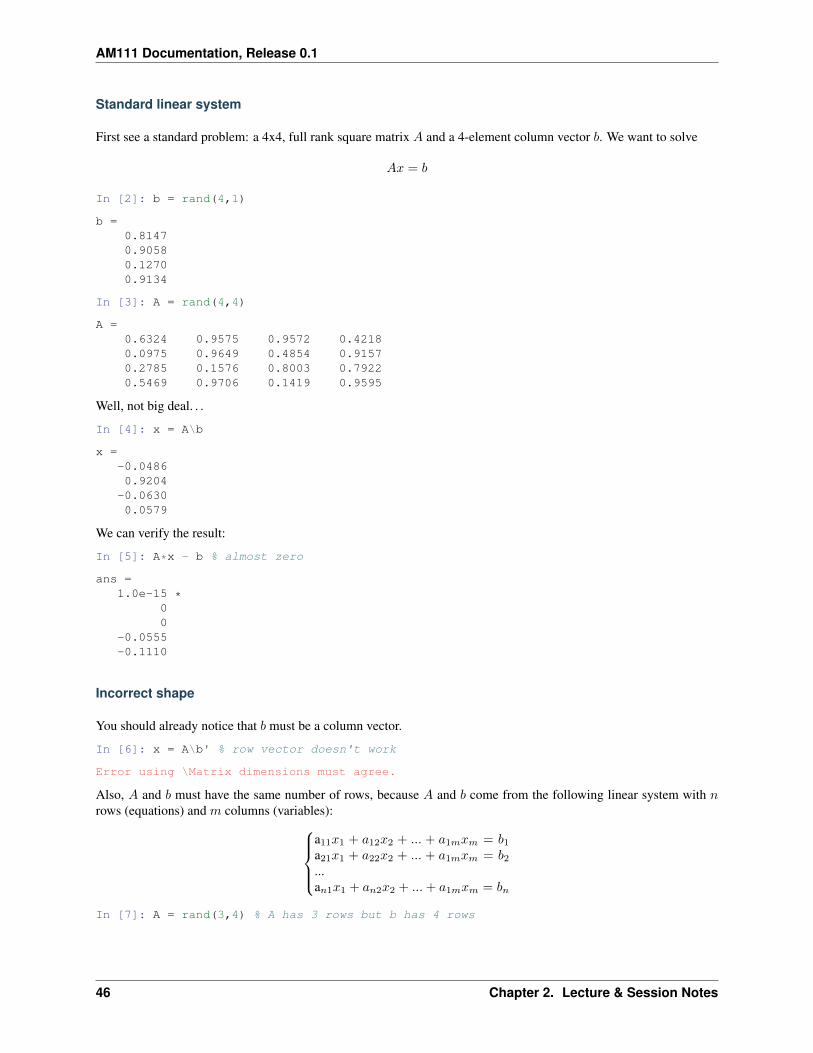
First see a standard problem: a 4x4, full rank square matrix 𝐴 and a 4-element column vector 𝑏. We want to solve
𝐴𝑥 = 𝑏
In [2]: b = rand(4,1)
b =0.81470.90580.12700.9134
In [3]: A = rand(4,4)
A =0.6324 0.9575 0.9572 0.42180.0975 0.9649 0.4854 0.91570.2785 0.1576 0.8003 0.79220.5469 0.9706 0.1419 0.9595
Well, not big deal. . .
In [4]: x = A\b
x =-0.04860.9204
-0.06300.0579
We can verify the result:
In [5]: A*x - b % almost zero
ans =1.0e-15 *
00
-0.0555-0.1110
Incorrect shape
You should already notice that 𝑏 must be a column vector.
In [6]: x = A\b' % row vector doesn't work
Error using \Matrix dimensions must agree.
Also, 𝐴 and 𝑏 must have the same number of rows, because 𝐴 and 𝑏 come from the following linear system with 𝑛rows (equations) and 𝑚 columns (variables):⎧⎪⎪⎨⎪⎪⎩
a11𝑥1 + 𝑎12𝑥2 + ... + 𝑎1𝑚𝑥𝑚 = 𝑏1a21𝑥1 + 𝑎22𝑥2 + ... + 𝑎1𝑚𝑥𝑚 = 𝑏2...a𝑛1𝑥1 + 𝑎𝑛2𝑥2 + ... + 𝑎1𝑚𝑥𝑚 = 𝑏𝑛
In [7]: A = rand(3,4) % A has 3 rows but b has 4 rows
46 Chapter 2. Lecture & Session Notes
AM111 Documentation, Release 0.1
A =0.6557 0.9340 0.7431 0.17120.0357 0.6787 0.3922 0.70600.8491 0.7577 0.6555 0.0318
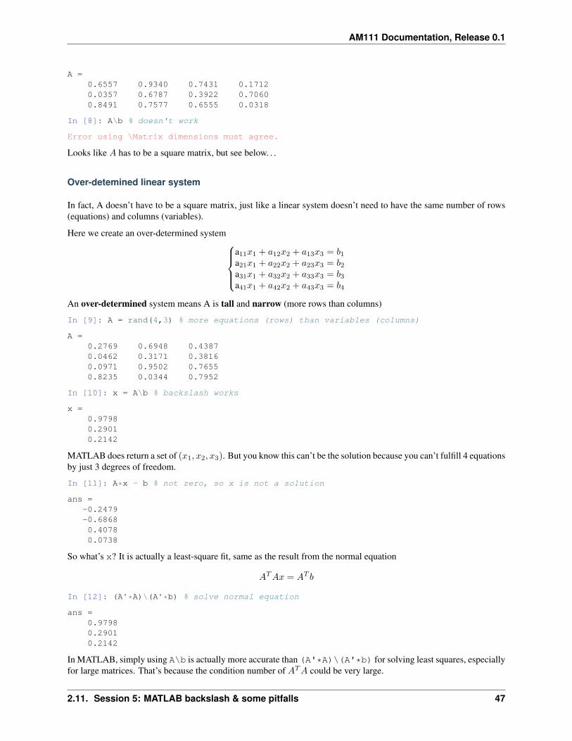
In [8]: A\b % doesn't work
Error using \Matrix dimensions must agree.
Looks like 𝐴 has to be a square matrix, but see below. . .
Over-detemined linear system
In fact, A doesn’t have to be a square matrix, just like a linear system doesn’t need to have the same number of rows(equations) and columns (variables).
Here we create an over-determined system⎧⎪⎪⎨⎪⎪⎩a11𝑥1 + 𝑎12𝑥2 + 𝑎13𝑥3 = 𝑏1a21𝑥1 + 𝑎22𝑥2 + 𝑎23𝑥3 = 𝑏2a31𝑥1 + 𝑎32𝑥2 + 𝑎33𝑥3 = 𝑏3a41𝑥1 + 𝑎42𝑥2 + 𝑎43𝑥3 = 𝑏4
An over-determined system means A is tall and narrow (more rows than columns)
In [9]: A = rand(4,3) % more equations (rows) than variables (columns)
A =0.2769 0.6948 0.43870.0462 0.3171 0.38160.0971 0.9502 0.76550.8235 0.0344 0.7952
In [10]: x = A\b % backslash works
x =0.97980.29010.2142
MATLAB does return a set of (𝑥1, 𝑥2, 𝑥3). But you know this can’t be the solution because you can’t fulfill 4 equationsby just 3 degrees of freedom.
In [11]: A*x - b % not zero, so x is not a solution
ans =-0.2479-0.68680.40780.0738
So what’s x? It is actually a least-square fit, same as the result from the normal equation
𝐴𝑇𝐴𝑥 = 𝐴𝑇 𝑏
In [12]: (A'*A)\(A'*b) % solve normal equation
ans =0.97980.29010.2142
In MATLAB, simply using A\b is actually more accurate than (A'*A)\(A'*b) for solving least squares, especiallyfor large matrices. That’s because the condition number of 𝐴𝑇𝐴 could be very large.
2.11. Session 5: MATLAB backslash & some pitfalls 47
AM111 Documentation, Release 0.1
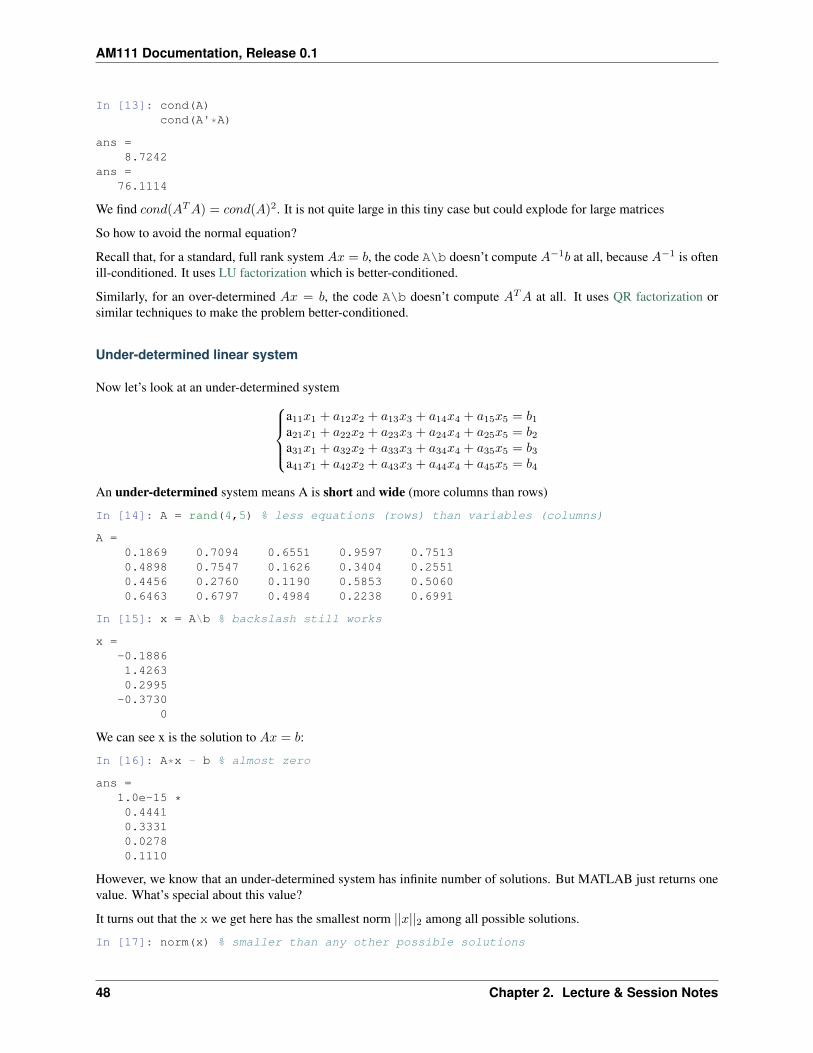
In [13]: cond(A)cond(A'*A)
ans =8.7242
ans =76.1114
We find 𝑐𝑜𝑛𝑑(𝐴𝑇𝐴) = 𝑐𝑜𝑛𝑑(𝐴)2. It is not quite large in this tiny case but could explode for large matrices
So how to avoid the normal equation?
Recall that, for a standard, full rank system 𝐴𝑥 = 𝑏, the code A\b doesn’t compute 𝐴−1𝑏 at all, because 𝐴−1 is oftenill-conditioned. It uses LU factorization which is better-conditioned.
Similarly, for an over-determined 𝐴𝑥 = 𝑏, the code A\b doesn’t compute 𝐴𝑇𝐴 at all. It uses QR factorization orsimilar techniques to make the problem better-conditioned.
Under-determined linear system
Now let’s look at an under-determined system⎧⎪⎪⎨⎪⎪⎩a11𝑥1 + 𝑎12𝑥2 + 𝑎13𝑥3 + 𝑎14𝑥4 + 𝑎15𝑥5 = 𝑏1a21𝑥1 + 𝑎22𝑥2 + 𝑎23𝑥3 + 𝑎24𝑥4 + 𝑎25𝑥5 = 𝑏2a31𝑥1 + 𝑎32𝑥2 + 𝑎33𝑥3 + 𝑎34𝑥4 + 𝑎35𝑥5 = 𝑏3a41𝑥1 + 𝑎42𝑥2 + 𝑎43𝑥3 + 𝑎44𝑥4 + 𝑎45𝑥5 = 𝑏4
An under-determined system means A is short and wide (more columns than rows)
In [14]: A = rand(4,5) % less equations (rows) than variables (columns)
A =0.1869 0.7094 0.6551 0.9597 0.75130.4898 0.7547 0.1626 0.3404 0.25510.4456 0.2760 0.1190 0.5853 0.50600.6463 0.6797 0.4984 0.2238 0.6991
In [15]: x = A\b % backslash still works
x =-0.18861.42630.2995
-0.37300
We can see x is the solution to 𝐴𝑥 = 𝑏:
In [16]: A*x - b % almost zero
ans =1.0e-15 *0.44410.33310.02780.1110
However, we know that an under-determined system has infinite number of solutions. But MATLAB just returns onevalue. What’s special about this value?
It turns out that the x we get here has the smallest norm ||𝑥||2 among all possible solutions.
In [17]: norm(x) % smaller than any other possible solutions
48 Chapter 2. Lecture & Session Notes
AM111 Documentation, Release 0.1
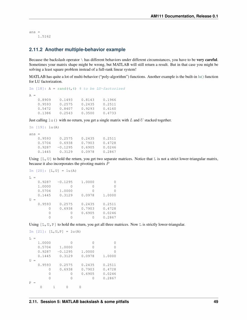
ans =1.5162
2.11.2 Another multiple-behavior example
Because the backslash operator \ has different behaviors under different circumstances, you have to be very careful.Sometimes your matrix shape might be wrong, but MATLAB will still return a result. But in that case you might besolving a least square problem instead of a full-rank linear system!
MATLAB has quite a lot of multi-behavior (“poly-algorithm”) functions. Another example is the built-in lu() functionfor LU factorization.
In [18]: A = rand(4,4) % to be LU-factorized
A =0.8909 0.1493 0.8143 0.19660.9593 0.2575 0.2435 0.25110.5472 0.8407 0.9293 0.61600.1386 0.2543 0.3500 0.4733
Just calling lu() with no return, you get a single matrix with 𝐿 and 𝑈 stacked together.
In [19]: lu(A)
ans =0.9593 0.2575 0.2435 0.25110.5704 0.6938 0.7903 0.47280.9287 -0.1295 0.6905 0.02460.1445 0.3129 0.0978 0.2867
Using [L,U] to hold the return, you get two separate matrices. Notice that L is not a strict lower-triangular matrix,because it also incorporates the pivoting matrix 𝑃
In [20]: [L,U] = lu(A)
L =0.9287 -0.1295 1.0000 01.0000 0 0 00.5704 1.0000 0 00.1445 0.3129 0.0978 1.0000
U =0.9593 0.2575 0.2435 0.2511
0 0.6938 0.7903 0.47280 0 0.6905 0.02460 0 0 0.2867
Using [L,U,P] to hold the return, you get all three matrices. Now L is strictly lower-triangular.
In [21]: [L,U,P] = lu(A)
L =1.0000 0 0 00.5704 1.0000 0 00.9287 -0.1295 1.0000 00.1445 0.3129 0.0978 1.0000
U =0.9593 0.2575 0.2435 0.2511
0 0.6938 0.7903 0.47280 0 0.6905 0.02460 0 0 0.2867
P =0 1 0 0
2.11. Session 5: MATLAB backslash & some pitfalls 49
AM111 Documentation, Release 0.1
0 0 1 01 0 0 00 0 0 1
You can ignore the returning P by ~, but keep in mind that the returning L is different from that in cell [20], althoughthe code looks very similar.
In [22]: [L,U,~] = lu(A)
L =1.0000 0 0 00.5704 1.0000 0 00.9287 -0.1295 1.0000 00.1445 0.3129 0.0978 1.0000
U =0.9593 0.2575 0.2435 0.2511
0 0.6938 0.7903 0.47280 0 0.6905 0.02460 0 0 0.2867
2.12 Session 6: Three ways of differentiation
Date: 10/23/2017, Monday
In [1]: format compact
There are 3 major ways to compute the derivative 𝑓 ′(𝑥)
• Symbolic differentiation
• Numerical differentiation
• Automatic differentiation
You are already familiar with the first two. The last one is not required by this class, but it is just too good to miss. Itis the core of modern deep learning engines like Google’s TensorFlow, which is used for training AlphaGo Zero. Herewe only give a very basic introduction. Enthusiasts can read Baydin A G, Pearlmutter B A, Radul A A, et al. Automaticdifferentiation in machine learning: a survey
Let’s compare the pros and cons of each method.
2.12.1 Symbolic differentiation
MATLAB toolbox
MATLAB provides symbolic tool box for symbolic differentiation. It can assist your mathetical analysis and can beused to verify the numerical differentiation results.
In [2]: syms x
Consider this function
𝑓(𝑥) =1 − 𝑒−𝑥
1 + 𝑒−𝑥
In [3]: f0 = (1-exp(-x))/(1+exp(-x))
f0 =-(exp(-x) - 1)/(exp(-x) + 1)
The first-order derivative is
50 Chapter 2. Lecture & Session Notes
AM111 Documentation, Release 0.1
In [4]: f1 = diff(f0,x)
f1 =exp(-x)/(exp(-x) + 1) - (exp(-x)*(exp(-x) - 1))/(exp(-x) + 1)ˆ2
We can keep calculating higher-order derivatives
In [5]: f2 = diff(f1,x)
f2 =(2*exp(-2*x))/(exp(-x) + 1)ˆ2 - exp(-x)/(exp(-x) + 1) + (exp(-x)*(exp(-x) - 1))/(exp(-x) + 1)ˆ2 - (2*exp(-2*x)*(exp(-x) - 1))/(exp(-x) + 1)ˆ3
In [6]: f3 = diff(f2,x)
f3 =exp(-x)/(exp(-x) + 1) - (6*exp(-2*x))/(exp(-x) + 1)ˆ2 + (6*exp(-3*x))/(exp(-x) + 1)ˆ3 - (exp(-x)*(exp(-x) - 1))/(exp(-x) + 1)ˆ2 + (6*exp(-2*x)*(exp(-x) - 1))/(exp(-x) + 1)ˆ3 - (6*exp(-3*x)*(exp(-x) - 1))/(exp(-x) + 1)ˆ4
In [7]: f4 = diff(f3,x)
f4 =(14*exp(-2*x))/(exp(-x) + 1)ˆ2 - exp(-x)/(exp(-x) + 1) - (36*exp(-3*x))/(exp(-x) + 1)ˆ3 + (24*exp(-4*x))/(exp(-x) + 1)ˆ4 + (exp(-x)*(exp(-x) - 1))/(exp(-x) + 1)ˆ2 - (14*exp(-2*x)*(exp(-x) - 1))/(exp(-x) + 1)ˆ3 + (36*exp(-3*x)*(exp(-x) - 1))/(exp(-x) + 1)ˆ4 - (24*exp(-4*x)*(exp(-x) - 1))/(exp(-x) + 1)ˆ5
In [8]: f5 = diff(f4,x)
f5 =exp(-x)/(exp(-x) + 1) - (30*exp(-2*x))/(exp(-x) + 1)ˆ2 + (150*exp(-3*x))/(exp(-x) + 1)ˆ3 - (240*exp(-4*x))/(exp(-x) + 1)ˆ4 + (120*exp(-5*x))/(exp(-x) + 1)ˆ5 - (exp(-x)*(exp(-x) - 1))/(exp(-x) + 1)ˆ2 + (30*exp(-2*x)*(exp(-x) - 1))/(exp(-x) + 1)ˆ3 - (150*exp(-3*x)*(exp(-x) - 1))/(exp(-x) + 1)ˆ4 + (240*exp(-4*x)*(exp(-x) - 1))/(exp(-x) + 1)ˆ5 - (120*exp(-5*x)*(exp(-x) - 1))/(exp(-x) + 1)ˆ6
We see the expression becomes more and more complicated for higher-order derivatives, even though the original 𝑓(𝑥)is fairly simple.
You can imagine that symbolic diff can be quite inefficient for complicated functions and higher-order derivatives.
Convert symbol to function
We can convert MATLAB symbols to functions, and use them to compute numerical values.
In [9]: f0_func = matlabFunction(f0)
f0_func =function_handle with value:
@(x)-(exp(-x)-1.0)./(exp(-x)+1.0)
f0 is converted to a normal MATLAB function. It is different from just copying the symbolic expression to MATLABcodes, as it is vectorized over input x (notice the ./).
Same for f0’s derivatives:
In [10]: f1_func = matlabFunction(f1);f2_func = matlabFunction(f2);f3_func = matlabFunction(f3);f4_func = matlabFunction(f4);f5_func = matlabFunction(f5);
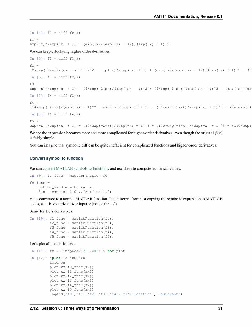
Let’s plot all the derivatives.
In [11]: xx = linspace(-3,3,40); % for plot
In [12]: %plot -s 400,300hold onplot(xx,f0_func(xx))plot(xx,f1_func(xx))plot(xx,f2_func(xx))plot(xx,f3_func(xx))plot(xx,f4_func(xx))plot(xx,f5_func(xx))legend('f0','f1','f2','f3','f4','f5','Location','SouthEast')
2.12. Session 6: Three ways of differentiation 51
AM111 Documentation, Release 0.1
2.12.2 Numerical differentiation
Is it possible to use the numerical differentiation we learned in class to approximate the 5-th order derivative? Let’stry.
In [13]: y0 = f0_func(xx); % get numerical data
In [14]: dx = xx(2)-xx(1) % get step size
dx =0.1538
We use the center difference, which is much more accurate than forward or backward difference.
𝑓 ′(𝑥) ≈ 𝑓(𝑥 + ℎ) − 𝑓(𝑥− ℎ)
2ℎ
For simplicity, we just throw away the end points x(1) and x(end). So the resulted gradient array y1 is shorterthan y0 by 2 elements. You can also use forward or backward diff to approximate the derivates at the end points. Buthere we only focus on internal points.
In [15]: y1 = (y0(3:end) - y0(1:end-2)) / (2*dx);length(y1)
ans =38
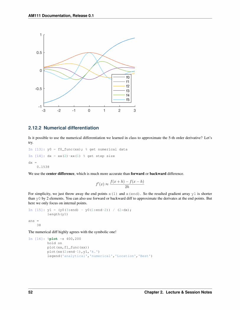
The numerical diff highly agrees with the symbolic one!
In [16]: %plot -s 400,200hold onplot(xx,f1_func(xx))plot(xx(2:end-1),y1,'k.')legend('analytical','numerical','Location','Best')
52 Chapter 2. Lecture & Session Notes

AM111 Documentation, Release 0.1
Then we go to 2-nd order:
In [17]: y2 = (y1(3:end) - y1(1:end-2)) / (2*dx);length(y2)
ans =36
In [18]: %plot -s 400,200hold onplot(xx,f2_func(xx))plot(xx(3:end-2),y2,'.k')
Also doing well. 3-rd order?
In [19]: y3 = (y2(3:end) - y2(1:end-2)) / (2*dx);length(y3)
ans =34
In [20]: %plot -s 400,200hold onplot(xx,f3_func(xx))plot(xx(4:end-3),y3,'.k')
2.12. Session 6: Three ways of differentiation 53
AM111 Documentation, Release 0.1
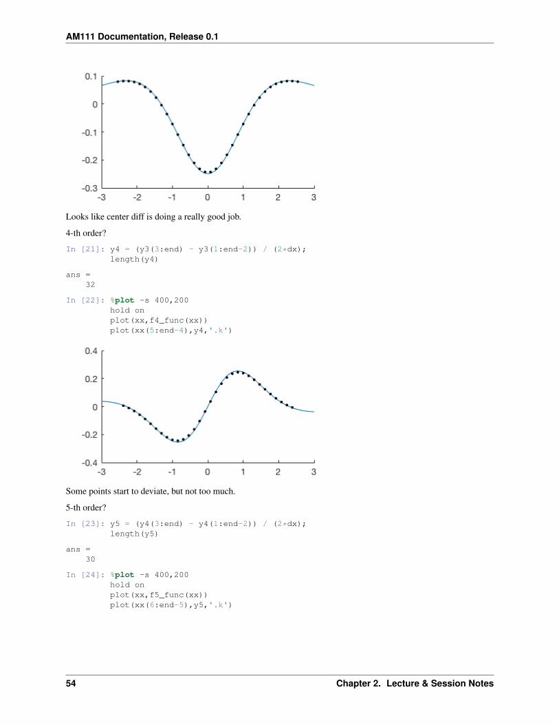
Looks like center diff is doing a really good job.
4-th order?
In [21]: y4 = (y3(3:end) - y3(1:end-2)) / (2*dx);length(y4)
ans =32
In [22]: %plot -s 400,200hold onplot(xx,f4_func(xx))plot(xx(5:end-4),y4,'.k')
Some points start to deviate, but not too much.
5-th order?
In [23]: y5 = (y4(3:end) - y4(1:end-2)) / (2*dx);length(y5)
ans =30
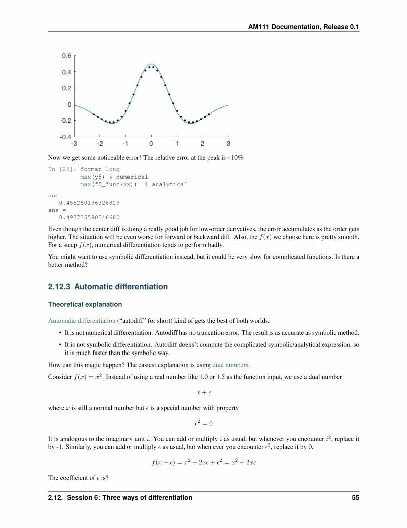
In [24]: %plot -s 400,200hold onplot(xx,f5_func(xx))plot(xx(6:end-5),y5,'.k')
54 Chapter 2. Lecture & Session Notes
AM111 Documentation, Release 0.1
Now we get some noticeable error! The relative error at the peak is ~10%.
In [25]: format longmax(y5) % numericalmax(f5_func(xx)) % analytical
ans =0.455250196326829
ans =0.493735580546680
Even though the center diff is doing a really good job for low-order derivatives, the error accumulates as the order getshigher. The situation will be even worse for forward or backward diff. Also, the 𝑓(𝑥) we choose here is pretty smooth.For a steep 𝑓(𝑥), numerical differentiation tends to perform badly.
You might want to use symbolic differentiation instead, but it could be very slow for complicated functions. Is there abetter method?
2.12.3 Automatic differentiation
Theoretical explanation
Automatic differentiation (“autodiff” for short) kind of gets the best of both worlds.
• It is not numerical differentiation. Autodiff has no truncation error. The result is as accurate as symbolic method.
• It is not symbolic differentiation. Autodiff doens’t compute the complicated symbolic/analytical expression, soit is much faster than the symbolic way.
How can this magic happen? The easiest explanation is using dual numbers.
Consider 𝑓(𝑥) = 𝑥2. Instead of using a real number like 1.0 or 1.5 as the function input, we use a dual number
𝑥 + 𝜖
where 𝑥 is still a normal number but 𝜖 is a special number with property
𝜖2 = 0
It is analogous to the imaginary unit 𝑖. You can add or multiply 𝑖 as usual, but whenever you encounter 𝑖2, replace itby -1. Similarly, you can add or multiply 𝜖 as usual, but when ever you encounter 𝜖2, replace it by 0.
𝑓(𝑥 + 𝜖) = 𝑥2 + 2𝑥𝜖 + 𝜖2 = 𝑥2 + 2𝑥𝜖
The coefficient of 𝜖 is?
2.12. Session 6: Three ways of differentiation 55
AM111 Documentation, Release 0.1
2𝑥 !! which is just 𝑓 ′(𝑥)
We didn’t perform any “differentiating” at all. Just by carrying an additional “number” 𝜖 through a function,we got the derivative of that function as well.
Let’s see another example 𝑓(𝑥) = 𝑥3
(𝑥 + 𝜖)3 = 𝑥3 + 3𝑥2𝜖 + 3𝑥𝜖2 + 𝜖3 = 𝑥3 + 3𝑥2𝜖
The coeffcient is 3𝑥2, which is just the derivative of 𝑥3.
If the function is not a polynomial? Say 𝑓(𝑥) = 𝑒𝑥
𝑒𝑥+𝜖 = 𝑒𝑥𝑒𝜖 = 𝑒𝑥(1 + 𝜖 +1
2𝜖2 + ...) = 𝑒𝑥(1 + 𝜖)
The coeffcient of 𝜖 is 𝑒𝑥, which is the derivative of 𝑒𝑥. (If you wonder how can a computer know the Taylor expansionof 𝑒𝜖, think about how can a computer calculate 𝑒𝑥)
Code example
MATLAB doesn’t have a good autodiff tool, so we use a Python package autograd developed by Harvard IntelligentProbabilistic Systems Group.
You don’t need to try this package right now (since this is not a Python class), but just keep in mind that if youneed a fast and accurate way to compute derivative, there are such tools exist.
Don’t worry if you don’t know Python. We will explain as it goes.
In [1]: %matplotlib inlineimport matplotlib.pyplot as plt # contains all plotting functionsimport autograd.numpy as np # contains all basic numerical functionsfrom autograd import grad # autodiff tool
We still differentiate 𝑓(𝑥) = 1−𝑒−𝑥
1+𝑒−𝑥 as in the MATLAB section.
In [2]: # Define a Python function# Python has no "end" statement# It uses code indentation to determine the end of each blockdef f0(x):
y = np.exp(-x)return (1.0 - y) / (1.0 + y)
In [3]: # grad(f0) returns the gradient of f0# f1 is not a symbolic expression!# It is just a normal numerical function,# but it returns the exact gradient thanks to the autodiff magicf1 = grad(f0)f2 = grad(f1)f3 = grad(f2)f4 = grad(f3)f5 = grad(f4)
In [4]: xx = np.linspace(-3, 3, 40) # for plot
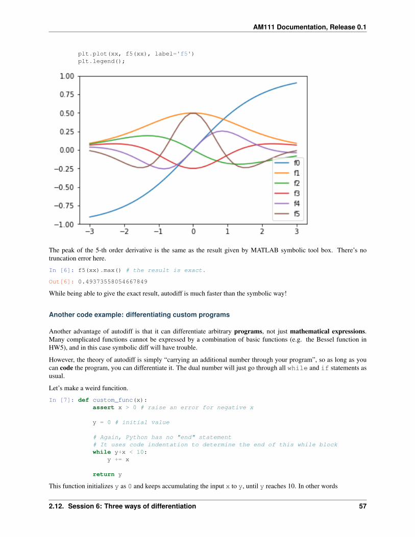
In [5]: # plot all derivatives# as in cell[12] of the MATLAB sectionplt.plot(xx, f0(xx), label='f0')plt.plot(xx, f1(xx), label='f1')plt.plot(xx, f2(xx), label='f2')plt.plot(xx, f3(xx), label='f3')plt.plot(xx, f4(xx), label='f4')
56 Chapter 2. Lecture & Session Notes
AM111 Documentation, Release 0.1
plt.plot(xx, f5(xx), label='f5')plt.legend();
The peak of the 5-th order derivative is the same as the result given by MATLAB symbolic tool box. There’s notruncation error here.
In [6]: f5(xx).max() # the result is exact.
Out[6]: 0.49373558054667849
While being able to give the exact result, autodiff is much faster than the symbolic way!
Another code example: differentiating custom programs
Another advantage of autodiff is that it can differentiate arbitrary programs, not just mathematical expressions.Many complicated functions cannot be expressed by a combination of basic functions (e.g. the Bessel function inHW5), and in this case symbolic diff will have trouble.
However, the theory of autodiff is simply “carrying an additional number through your program”, so as long as youcan code the program, you can differentiate it. The dual number will just go through all while and if statements asusual.
Let’s make a weird funcition.
In [7]: def custom_func(x):assert x > 0 # raise an error for negative x
y = 0 # initial value
# Again, Python has no "end" statement# It uses code indentation to determine the end of this while blockwhile y+x < 10:
y += x
return y
This function initializes y as 0 and keeps accumulating the input x to y, until y reaches 10. In other words
2.12. Session 6: Three ways of differentiation 57
AM111 Documentation, Release 0.1
• y is a multiple of x, i.e. y=N*x.
• y is smaller than but very close to 10
For 𝑥 = 1, 𝑓(𝑥) = 9𝑥 = 9, because 10𝑥 will exceed 10.
In [8]: custom_func(1.0)
Out[8]: 9.0
For 𝑥 = 1.2, 𝑓(𝑥) = 8𝑥 = 9.6, because 9𝑥 = 10.8 will exceed 10.
In [9]: custom_func(1.2)
Out[9]: 9.6
We can still take derivative of this weird function.
In [10]: custom_grad = grad(custom_func) # autodiff magic
For 𝑥 = 1, 𝑓(𝑥) = 9𝑥, so 𝑓 ′(𝑥) = 9
In [11]: print(custom_grad(1.0))
9.0
For 𝑥 = 1.2, 𝑓(𝑥) = 8𝑥, so 𝑓 ′(𝑥) = 8
In [12]: print(custom_grad(1.2))
8.0
Symbolic diff will have a big trouble with this kind of function.
2.12.4 So why use numerical differentiation?
If autodiff is so powerful, why do we need other methods? Well, you need symbolic diff for pure mathematicalanalysis. But how about numerical diff?
Well, the major application of numerical diff (forward difference, etc.) is not getting the derivative of a known function𝑓(𝑥). It is for solving differential equations
𝑓 ′(𝑥) = Φ(𝑓, 𝑥)
In this case, 𝑓(𝑥) is not known (your goal is to find it), so symbol diff or autodiff can’t help you. Numerical diff givesyou a way to solve this ODE
𝑓(𝑥 + ℎ) − 𝑓(𝑥)
ℎ≈ 𝑓 ′(𝑥) = Φ(𝑓, 𝑥)
2.13 Session 7: Error convergence of numerical methods
Date: 10/30/2017, Monday
In [1]: format compact
58 Chapter 2. Lecture & Session Notes
AM111 Documentation, Release 0.1
2.13.1 Error convergence of general numerical methods
Many numerical methods has a “step size” or “interval size” ℎ, no mattter numerical differentiation, numerical inter-gration or ODE solving. We denote 𝑓(ℎ) as the numerical approximation to the exact answer 𝑓𝑡𝑟𝑢𝑒. Note that 𝑓 canbe a derivate, an integral or an ODE solution.
In general, the numerical error gets smaller when ℎ is reduced. We say a method has 𝑂(ℎ𝑘) convergence if
𝑓(ℎ) − 𝑓𝑡𝑟𝑢𝑒 = 𝐶 · ℎ𝑘 + 𝐶1 · ℎ𝑘+1 + ...
As ℎ → 0, we will have 𝑓(ℎ) → 𝑓𝑡𝑟𝑢𝑒. Higher-order methods (i.e. larger 𝑘) leads to faster convergence.
2.13.2 Error convergence of numerical differentiation
Consider 𝑓(𝑥) = 𝑒𝑥, we use finite difference to approximate 𝑔(𝑥) = 𝑓 ′(𝑥) = 𝑒𝑥. We only consider 𝑥 = 1 here.
In [2]: f = @(x) exp(x); % the function we want to differentiate
In [3]: x0 = 1; % only consider this pointg_true = exp(x0) % analytical solution
g_true =2.7183
We try both forward and center schemes, with different step sizes ℎ.
In [4]: h_list = 0.01:0.01:0.1; % test different step size hn = length(h_list);g_forward = zeros(1,n); % to hold forward difference resultsg_center = zeros(1,n); % to hold center difference results
for i = 1:n % loop over different step sizesh = h_list(i); % get step size
% forward differenceg_forward(i) = (f(x0+h) - f(x0))/h;
% center differenceg_center(i) = (f(x0+h) - f(x0-h))/(2*h);
end
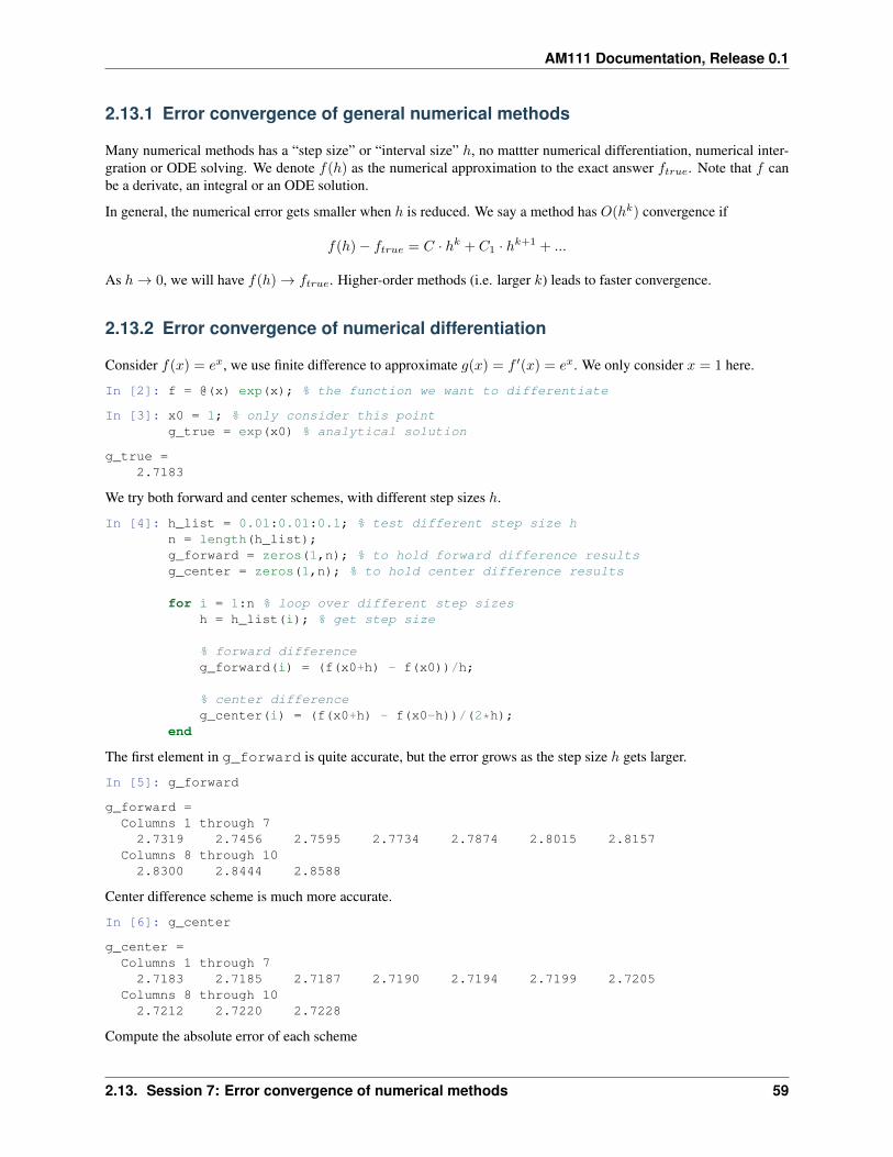
The first element in g_forward is quite accurate, but the error grows as the step size ℎ gets larger.
In [5]: g_forward
g_forward =Columns 1 through 72.7319 2.7456 2.7595 2.7734 2.7874 2.8015 2.8157
Columns 8 through 102.8300 2.8444 2.8588
Center difference scheme is much more accurate.
In [6]: g_center
g_center =Columns 1 through 72.7183 2.7185 2.7187 2.7190 2.7194 2.7199 2.7205
Columns 8 through 102.7212 2.7220 2.7228
Compute the absolute error of each scheme
2.13. Session 7: Error convergence of numerical methods 59
AM111 Documentation, Release 0.1
In [7]: error_forward = abs(g_forward - g_true)error_center = abs(g_center - g_true)
error_forward =Columns 1 through 70.0136 0.0274 0.0412 0.0551 0.0691 0.0832 0.0974
Columns 8 through 100.1117 0.1261 0.1406
error_center =Columns 1 through 70.0000 0.0002 0.0004 0.0007 0.0011 0.0016 0.0022
Columns 8 through 100.0029 0.0037 0.0045
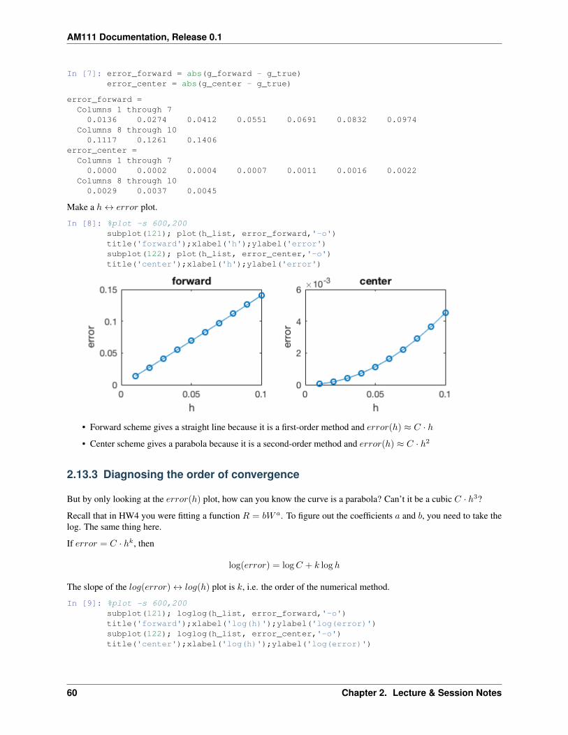
Make a ℎ ↔ 𝑒𝑟𝑟𝑜𝑟 plot.
In [8]: %plot -s 600,200subplot(121); plot(h_list, error_forward,'-o')title('forward');xlabel('h');ylabel('error')subplot(122); plot(h_list, error_center,'-o')title('center');xlabel('h');ylabel('error')
• Forward scheme gives a straight line because it is a first-order method and 𝑒𝑟𝑟𝑜𝑟(ℎ) ≈ 𝐶 · ℎ
• Center scheme gives a parabola because it is a second-order method and 𝑒𝑟𝑟𝑜𝑟(ℎ) ≈ 𝐶 · ℎ2
2.13.3 Diagnosing the order of convergence
But by only looking at the 𝑒𝑟𝑟𝑜𝑟(ℎ) plot, how can you know the curve is a parabola? Can’t it be a cubic 𝐶 · ℎ3?
Recall that in HW4 you were fitting a function 𝑅 = 𝑏𝑊 𝑎. To figure out the coefficients 𝑎 and 𝑏, you need to take thelog. The same thing here.
If 𝑒𝑟𝑟𝑜𝑟 = 𝐶 · ℎ𝑘, then
log(𝑒𝑟𝑟𝑜𝑟) = log𝐶 + 𝑘 log ℎ
The slope of the 𝑙𝑜𝑔(𝑒𝑟𝑟𝑜𝑟) ↔ 𝑙𝑜𝑔(ℎ) plot is 𝑘, i.e. the order of the numerical method.
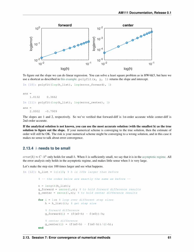
In [9]: %plot -s 600,200subplot(121); loglog(h_list, error_forward,'-o')title('forward');xlabel('log(h)');ylabel('log(error)')subplot(122); loglog(h_list, error_center,'-o')title('center');xlabel('log(h)');ylabel('log(error)')
60 Chapter 2. Lecture & Session Notes
AM111 Documentation, Release 0.1
To figure out the slope we can do linear regression. You can solve a least square problem as in HW4&5, but here weuse a shortcut as described in this example. polyfit(x, y, 1) returns the slope and intercept.
In [10]: polyfit(log(h_list), log(error_forward), 1)
ans =1.0132 0.3662
In [11]: polyfit(log(h_list), log(error_center), 1)
ans =2.0002 -0.7909
The slopes are 1 and 2, respectively. So we’ve verified that forward-diff is 1st-order accurate while center-diff is2nd-order accurate.
If the analytical solution is not known, you can use the most accurate solution (with the smallest h) as the truesolution to figure out the slope. If your numerical scheme is converging to the true solution, then the estimate oforder will still be OK. The risk is your numerical scheme might be converging to a wrong solution, and in this case itmakes no sense to talk about error convergence.
2.13.4 ℎ needs to be small
𝑒𝑟𝑟𝑜𝑟(ℎ) ≈ 𝐶 · ℎ𝑘 only holds for small ℎ. When ℎ is sufficiently small, we say that it is in the asymptotic regime. Allthe error analysis only holds in the asymptotic regime, and makes little sense when ℎ is very large.
Let’s make the step size 100 times larger and see what happens.
In [12]: h_list = 1:1:10; % h is 100x larger than before
% -- the codes below are exactly the same as before --
n = length(h_list);g_forward = zeros(1,n); % to hold forward difference resultsg_center = zeros(1,n); % to hold center difference results
for i = 1:n % loop over different step sizesh = h_list(i); % get step size
% forward differenceg_forward(i) = (f(x0+h) - f(x0))/h;
% center differenceg_center(i) = (f(x0+h) - f(x0-h))/(2*h);
end
2.13. Session 7: Error convergence of numerical methods 61

AM111 Documentation, Release 0.1
error_forward = abs(g_forward - g_true);error_center = abs(g_center - g_true);
In [13]: %plot -s 600,200subplot(121); loglog(h_list, error_forward,'-o')title('forward');xlabel('log(h)');ylabel('log(error)')subplot(122); loglog(h_list, error_center,'-o')title('center');xlabel('log(h)');ylabel('log(error)')
Now the error is super large and the log-log plot is not a straight line. So keep in mind that for most numerical schemeswe always assume small ℎ.
So how small is “small”? It depends on the scale of your problem and how rapidly 𝑓(𝑥) changes. If the problem isdefined in 𝑥 ∈ [0, 0.001], then ℎ = 0.001 is not small at all!
2.13.5 Error convergence of numerical intergration
Now consider
𝐼 =
∫ 1
0
𝑓(𝑥)
We still use 𝑓(𝑥) = 𝑒𝑥 for convenience, as the integral of 𝑒𝑥 is still 𝑒𝑥.
In [14]: f = @(x) exp(x); % the function we want to integrate
In [15]: I_true = exp(1)-exp(0)
I_true =1.7183
We use composite midpoint scheme to approximate 𝐼 . We test different interval size ℎ. Note that we need to firstdefine the number of intervals 𝑚, and then get the corresponding ℎ, because 𝑚 has to be an integer.
In [16]: m_list = 10:10:100; % number of pointsh_list = 1./m_list; % interval size
n = length(m_list);I_list = zeros(1,n); % to hold intergration results
for i=1:n % loop over different interval sizes (or number of intevals)m = m_list(i);h = h_list(i);
% get edge points
62 Chapter 2. Lecture & Session Notes
AM111 Documentation, Release 0.1
x_edge = linspace(0, 1, m+1);
% edge to middlex_mid = (x_edge(1:end-1) + x_edge(2:end))/2;
% composite midpoint intergration schemeI_list(i) = h*sum(f(x_mid));
end
The result is quite accurate.
In [17]: I_list
I_list =Columns 1 through 71.7176 1.7181 1.7182 1.7182 1.7183 1.7183 1.7183
Columns 8 through 101.7183 1.7183 1.7183
The error is at the order of 10−3.
In [18]: error_I = abs(I_list-I_true)
error_I =1.0e-03 *Columns 1 through 70.7157 0.1790 0.0795 0.0447 0.0286 0.0199 0.0146
Columns 8 through 100.0112 0.0088 0.0072
Again, a log-log plot will provide more insights about the order of convergence.
In [19]: %plot -s 600,200subplot(121);plot(h_list, error_I, '-o')title('error -- h');xlabel('h');ylabel('error')subplot(122);loglog(h_list, error_I, '-o')title('log(error) -- log(h)');xlabel('log(h)');ylabel('log(error)')
The slope is 2, so the method is second order accurate.
In [20]: polyfit(log(h_list), log(error_I), 1)
ans =1.9999 -2.6372
We’ve just applied the same error analysis method on both differentiation and integration. The same methodalso applies to ODE solving.
2.13. Session 7: Error convergence of numerical methods 63
AM111 Documentation, Release 0.1
2.13.6 Error convergence of ODE solving
Consider a simple ODE
𝑑𝑦(𝑡)
𝑑𝑡= 𝑦(𝑡), 𝑦(0) = 1
The exact solution is 𝑦(𝑡) = 𝑒𝑡. We use the forward Euler scheme to solve it.
𝑦(𝑡 + ℎ) − 𝑦(𝑡)
ℎ≈ 𝑦(𝑡)
The iteration is given by
𝑦(𝑡 + ℎ) = 𝑦(𝑡) + ℎ · 𝑦(𝑡) = (1 + ℎ)𝑦(𝑡)
Let’s only consider 𝑡 ∈ [0, 1]. More specifically, we’ll only look at the final state 𝑦(1), so we don’t need to recordevery step.
In [21]: y1_true = exp(1) % true y(1)
y1_true =2.7183
Same as in the integration section, we need to first define the number of total iterations 𝑚, and then get the corre-sponding step size ℎ. This ensures we will land exactly at 𝑡 = 1, not its neighbours.
In [22]: y0 = 1; % initial condition
m_list = 10:10:100; % number of iterations to get to t=1h_list = 1./m_list; % step size
n = length(m_list);y1_list = zeros(1,n); % to hold the final point
for i=1:n % loop over different step sizesm = m_list(i); % get the number of iterationsh = h_list(i); % get step size
y1 = y0; % start with y(0)
% Euler scheme begins herefor t=1:m
y1 = (1+h)*y1; % no need to record intermediate results hereend
y1_list(i) = y1; % only record the final point
end
As ℎ shrinks, our simulated 𝑦(1) gets closer to the true result.
In [23]: y1_list
y1_list =Columns 1 through 72.5937 2.6533 2.6743 2.6851 2.6916 2.6960 2.6991
Columns 8 through 102.7015 2.7033 2.7048
In [24]: error_y1 = abs(y1_list-y1_true)
64 Chapter 2. Lecture & Session Notes

AM111 Documentation, Release 0.1
error_y1 =Columns 1 through 70.1245 0.0650 0.0440 0.0332 0.0267 0.0223 0.0192
Columns 8 through 100.0168 0.0149 0.0135
𝑒𝑟𝑟𝑜𝑟 ↔ ℎ plot is a straight line, so we know the method is fist order accurate. The log-log plot is not quite necessaryhere.
In [25]: %plot -s 600,200subplot(121);plot(h_list, error_y1, '-o')title('error -- h');xlabel('h');ylabel('error')subplot(122);loglog(h_list, error_y1, '-o')title('log(error) -- log(h)');xlabel('log(h)');ylabel('log(error)')
Of course we can still calculate the slope of the log-log plot, to double check the forward Euler scheme is a first-ordermethod.
In [26]: polyfit(log(h_list), log(error_y1), 1)
ans =0.9687 0.1613
The take-away is, you can think about the order of a method in a more general sense. We’ve covered numericaldifferentiation, intergration and ODE here, and similar analysis also applies to root-finding, PDE, optimization,etc. . .
2.14 Session 8: ODE stability; stiff system
Date: 11/06/2017, Monday
In [1]: format compact
2.14.1 ODE Stability
Problem statement
Consider a simple ODE
𝑑𝑦
𝑑𝑡= −𝑎𝑦, 𝑦(0) = 𝑦0
where 𝑎 is a positive real number.
2.14. Session 8: ODE stability; stiff system 65
AM111 Documentation, Release 0.1
It can be solved analytically:
𝑦(𝑡) = 𝑦0𝑒−𝑎𝑡
So the analytical solution decays exponentially. A numerical solution is allowed to have some error, but it should alsobe decaying. If the solution is instead growing, we say it is unstable.
Explicit scheme
Forward Eulerian scheme for this problem is
𝑦𝑘+1 − 𝑦𝑘ℎ
= −𝑎𝑦𝑘
The iteration is given by
𝑦𝑘+1 = (1 − ℎ𝑎)𝑦𝑘
The solution at the k-th time step can be written out explicitly
𝑦𝑘 = (1 − ℎ𝑎)𝑘𝑦0
We all know that when ℎ gets smaller the numerical solution will converge to the true result. But here we are interestedin relatively large ℎ, i.e. we wonder what’s the largest possible ℎ we can use while still getting an OK result.
Here are the solutions with different ℎ.
In [2]: %plot -s 400,300
% set parameters, can use different valuea = 1;y0 = 1;tspan = 10;
% build functionf_true = @(t) y0*exp(-a*t); % true answerf_forward = @(k,h) (1-h*a).^k * y0; % forward Euler solution
% plot true resultt_ar = linspace(0, tspan); % for plottingy_true = f_true(t_ar);plot(t_ar, y_true)hold on
% plot Forward Euler solutionfor h=[2.5, 1.5, 0.5] % try different step size
kmax = round(tspan/h);k_ar = 0:kmax;t_ar = k_ar*h;
% we are not doing Forward Euler iteration here% since the expression is known, we can directly% get the entire time seriesy_forward = f_forward(k_ar, h);
plot(t_ar, y_forward, '-o')end
66 Chapter 2. Lecture & Session Notes
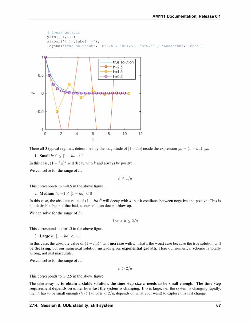
AM111 Documentation, Release 0.1
% tweak detailsylim([-1,1]);xlabel('t');ylabel('y');legend('true solution', 'h=2.5', 'h=1.5', 'h=0.5' , 'Location', 'Best')
There all 3 typical regimes, determined by the magnitude of [1 − ℎ𝑎] inside the expression 𝑦𝑘 = (1 − ℎ𝑎)𝑘𝑦0.
1. Small ℎ: 0 ≤ [1 − ℎ𝑎] < 1
In this case, (1 − ℎ𝑎)𝑘 will decay with 𝑘 and always be positve.
We can solve for the range of ℎ:
ℎ ≤ 1/𝑎
This corresponds to h=0.5 in the above figure.
2. Medium ℎ: −1 ≤ [1 − ℎ𝑎] < 0
In this case, the absolute value of (1 − ℎ𝑎)𝑘 will decay with 𝑘, but it oscillates between negative and postive. This isnot desirable, but not that bad, as our solution doesn’t blow up.
We can solve for the range of ℎ:
1/𝑎 < ℎ ≤ 2/𝑎
This corresponds to h=1.5 in the above figure.
3. Large ℎ: [1 − ℎ𝑎] < −1
In this case, the absolute value of (1 − ℎ𝑎)𝑘 will increase with 𝑘. That’s the worst case because the true solution willbe decaying, but our numerical solution insteads gives exponential growth. Here our numerical scheme is totallywrong, not just inaccurate.
We can solve for the range of ℎ:
ℎ > 2/𝑎
This corresponds to h=2.5 in the above figure.
The take-away is, to obtain a stable solution, the time step size ℎ needs to be small enough. The time steprequirement depends on 𝑎, i.e. how fast the system is changing. If 𝑎 is large, i.e. the system is changing rapidly,then ℎ has to be small enough (ℎ < 1/𝑎 or ℎ < 2/𝑎, depends on what your want) to capture this fast change.
2.14. Session 8: ODE stability; stiff system 67
AM111 Documentation, Release 0.1
Implicit scheme
But sometimes we really want to use a large step size. For example, we might only care about the steady state where 𝑡is very large, so we would like to quickly jump to the steady state with very few number of iterations. Implicit methodallows us to use a large time step while still keep the solution stable.
Backward Eulerian scheme for this problem is
𝑦𝑘+1 − 𝑦𝑘ℎ
= −𝑎𝑦𝑘+1
In general, the right hand-side would be some function 𝑓(𝑦𝑘+1), and we need to solve a nonlinear equation to obtain𝑦𝑘+1. This is why this method is called implicit. But in this problem here we happen to have a linear function, so wecan still write out the iteration explicitly.
𝑦𝑘+1 =𝑦𝑘
1 + ℎ𝑎
The solution at the k-th time step can be written as
𝑦𝑘 =𝑦0
(1 + ℎ𝑎)𝑘
Here are the solutions with different ℎ.
In [3]: %plot -s 400,300
% set parameters, can use different valuea = 1;y0 = 1;tspan = 10;
% build functionf_true = @(t) y0*exp(-a*t); % true answerf_backward = @(k,h) (1+h*a).^(-k) * y0; % backward Euler solution
% plot true resultt_ar = linspace(0, tspan); % for plottingy_true = f_true(t_ar);plot(t_ar, y_true)hold on
% plot Forward Euler solutionfor h=[2.5, 1.5, 0.5] % try different step size
kmax = round(tspan/h);k_ar = 0:kmax;t_ar = k_ar*h;
% we are not doing Forward Euler iteration here% since the expression is known, we can directly% get the entire time seriesy_backward = f_backward(k_ar, h);
plot(t_ar, y_backward, '-o')end
% tweak detailsylim([-0.2,1]);xlabel('t');ylabel('y');legend('true solution', 'h=2.5', 'h=1.5', 'h=0.5' , 'Location', 'Best')
68 Chapter 2. Lecture & Session Notes
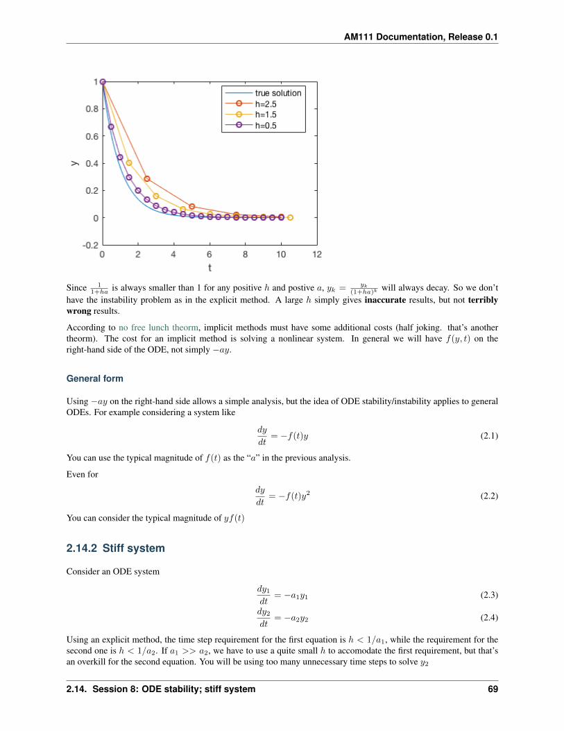
AM111 Documentation, Release 0.1
Since 11+ℎ𝑎 is always smaller than 1 for any positive ℎ and postive 𝑎, 𝑦𝑘 = 𝑦𝑘
(1+ℎ𝑎)𝑘will always decay. So we don’t
have the instability problem as in the explicit method. A large ℎ simply gives inaccurate results, but not terriblywrong results.
According to no free lunch theorm, implicit methods must have some additional costs (half joking. that’s anothertheorm). The cost for an implicit method is solving a nonlinear system. In general we will have 𝑓(𝑦, 𝑡) on theright-hand side of the ODE, not simply −𝑎𝑦.
General form
Using −𝑎𝑦 on the right-hand side allows a simple analysis, but the idea of ODE stability/instability applies to generalODEs. For example considering a system like
𝑑𝑦
𝑑𝑡= −𝑓(𝑡)𝑦 (2.1)
You can use the typical magnitude of 𝑓(𝑡) as the “𝑎” in the previous analysis.
Even for
𝑑𝑦
𝑑𝑡= −𝑓(𝑡)𝑦2 (2.2)
You can consider the typical magnitude of 𝑦𝑓(𝑡)
2.14.2 Stiff system
Consider an ODE system
𝑑𝑦1𝑑𝑡
= −𝑎1𝑦1 (2.3)
𝑑𝑦2𝑑𝑡
= −𝑎2𝑦2 (2.4)
Using an explicit method, the time step requirement for the first equation is ℎ < 1/𝑎1, while the requirement for thesecond one is ℎ < 1/𝑎2. If 𝑎1 >> 𝑎2, we have to use a quite small ℎ to accomodate the first requirement, but that’san overkill for the second equation. You will be using too many unnecessary time steps to solve 𝑦2
2.14. Session 8: ODE stability; stiff system 69
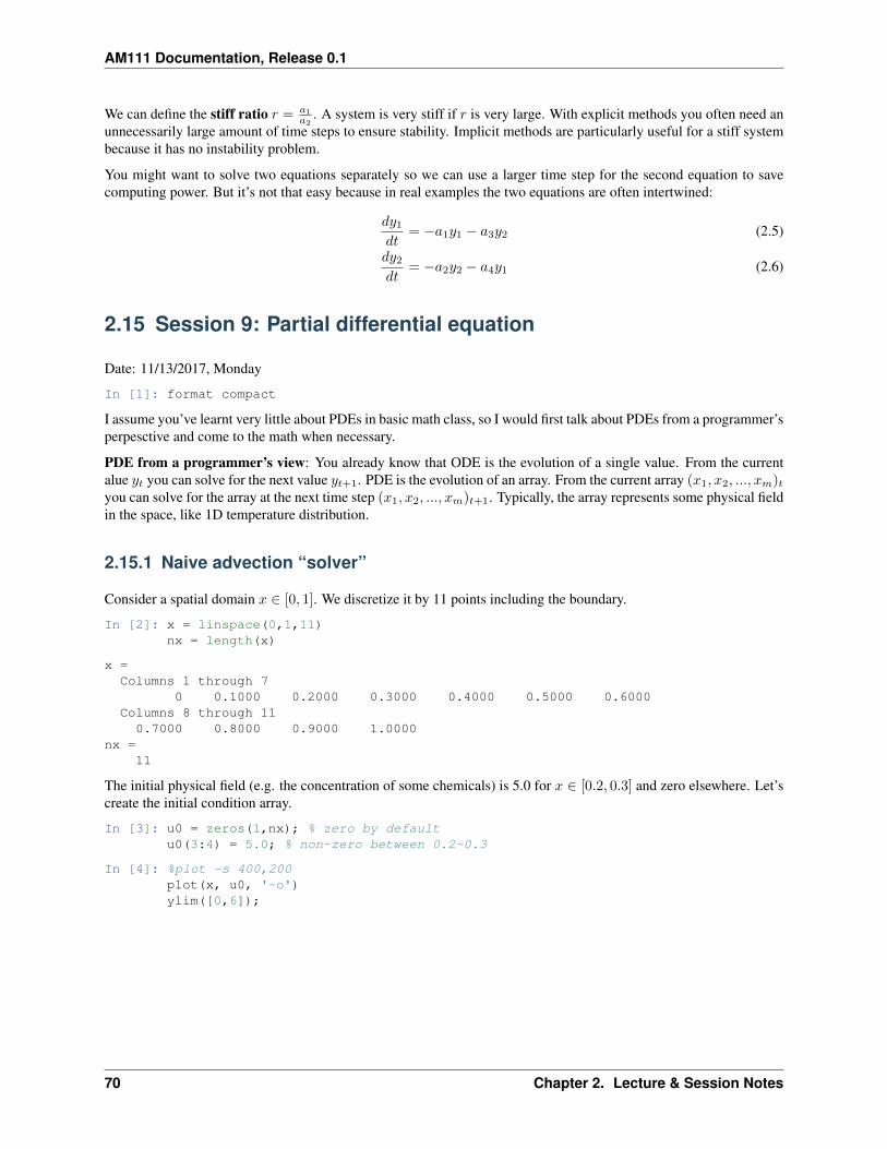
AM111 Documentation, Release 0.1
We can define the stiff ratio 𝑟 = 𝑎1
𝑎2. A system is very stiff if 𝑟 is very large. With explicit methods you often need an
unnecessarily large amount of time steps to ensure stability. Implicit methods are particularly useful for a stiff systembecause it has no instability problem.
You might want to solve two equations separately so we can use a larger time step for the second equation to savecomputing power. But it’s not that easy because in real examples the two equations are often intertwined:
𝑑𝑦1𝑑𝑡
= −𝑎1𝑦1 − 𝑎3𝑦2 (2.5)
𝑑𝑦2𝑑𝑡
= −𝑎2𝑦2 − 𝑎4𝑦1 (2.6)
2.15 Session 9: Partial differential equation
Date: 11/13/2017, Monday
In [1]: format compact
I assume you’ve learnt very little about PDEs in basic math class, so I would first talk about PDEs from a programmer’sperpesctive and come to the math when necessary.
PDE from a programmer’s view: You already know that ODE is the evolution of a single value. From the currentalue 𝑦𝑡 you can solve for the next value 𝑦𝑡+1. PDE is the evolution of an array. From the current array (𝑥1, 𝑥2, ..., 𝑥𝑚)𝑡you can solve for the array at the next time step (𝑥1, 𝑥2, ..., 𝑥𝑚)𝑡+1. Typically, the array represents some physical fieldin the space, like 1D temperature distribution.
2.15.1 Naive advection “solver”
Consider a spatial domain 𝑥 ∈ [0, 1]. We discretize it by 11 points including the boundary.
In [2]: x = linspace(0,1,11)nx = length(x)
x =Columns 1 through 7
0 0.1000 0.2000 0.3000 0.4000 0.5000 0.6000Columns 8 through 110.7000 0.8000 0.9000 1.0000
nx =11
The initial physical field (e.g. the concentration of some chemicals) is 5.0 for 𝑥 ∈ [0.2, 0.3] and zero elsewhere. Let’screate the initial condition array.
In [3]: u0 = zeros(1,nx); % zero by defaultu0(3:4) = 5.0; % non-zero between 0.2~0.3
In [4]: %plot -s 400,200plot(x, u0, '-o')ylim([0,6]);
70 Chapter 2. Lecture & Session Notes
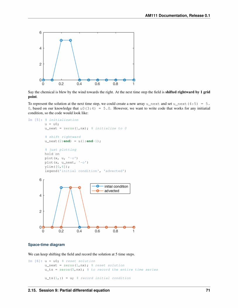
AM111 Documentation, Release 0.1
Say the chemical is blew by the wind towards the right. At the next time step the field is shifted rightward by 1 gridpoint.
To represent the solution at the next time step, we could create a new array u_next and set u_next(4:5) = 5.0, based on our knowledge that u0(3:4) = 5.0. However, we want to write code that works for any initiatialcondition, so the code would look like:
In [5]: % initializationu = u0;u_next = zeros(1,nx); % initialize to 0
% shift rightwardu_next(2:end) = u(1:end-1);
% just plottinghold onplot(x, u, '-o')plot(x, u_next, '-o')ylim([0,6]);legend('initial condition', 'advected')
Space-time diagram
We can keep shifting the field and record the solution at 5 time steps.
In [6]: u = u0; % reset solutionu_next = zeros(1,nx); % reset solutionu_ts = zeros(5,nx); % to record the entire time series
u_ts(1,:) = u; % record initial condition
2.15. Session 9: Partial differential equation 71
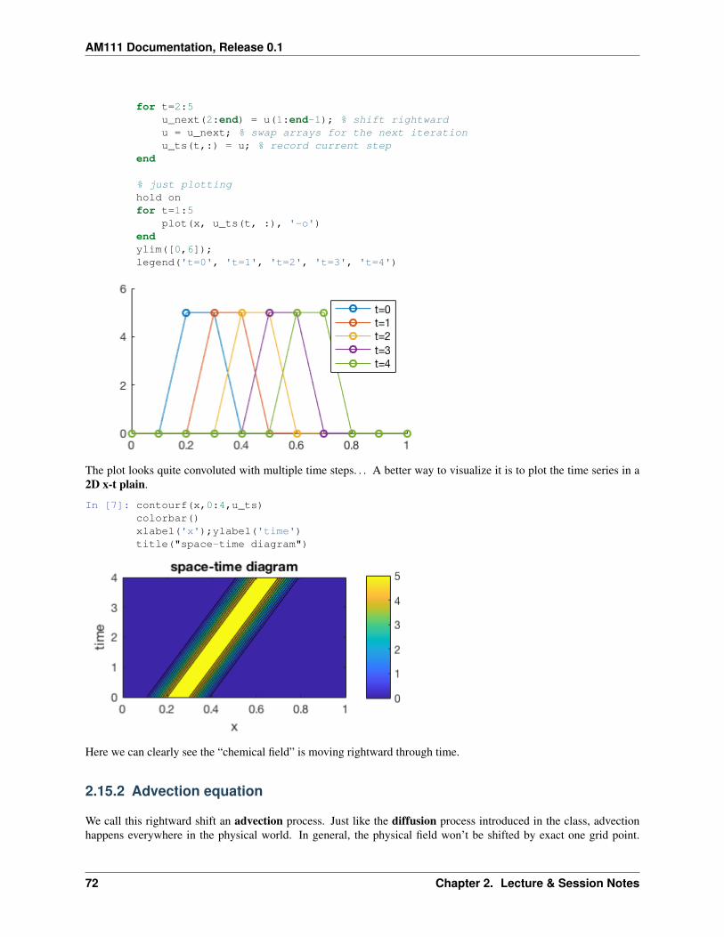
AM111 Documentation, Release 0.1
for t=2:5u_next(2:end) = u(1:end-1); % shift rightwardu = u_next; % swap arrays for the next iterationu_ts(t,:) = u; % record current step
end
% just plottinghold onfor t=1:5
plot(x, u_ts(t, :), '-o')endylim([0,6]);legend('t=0', 't=1', 't=2', 't=3', 't=4')
The plot looks quite convoluted with multiple time steps. . . A better way to visualize it is to plot the time series in a2D x-t plain.
In [7]: contourf(x,0:4,u_ts)colorbar()xlabel('x');ylabel('time')title("space-time diagram")
Here we can clearly see the “chemical field” is moving rightward through time.
2.15.2 Advection equation
We call this rightward shift an advection process. Just like the diffusion process introduced in the class, advectionhappens everywhere in the physical world. In general, the physical field won’t be shifted by exact one grid point.
72 Chapter 2. Lecture & Session Notes
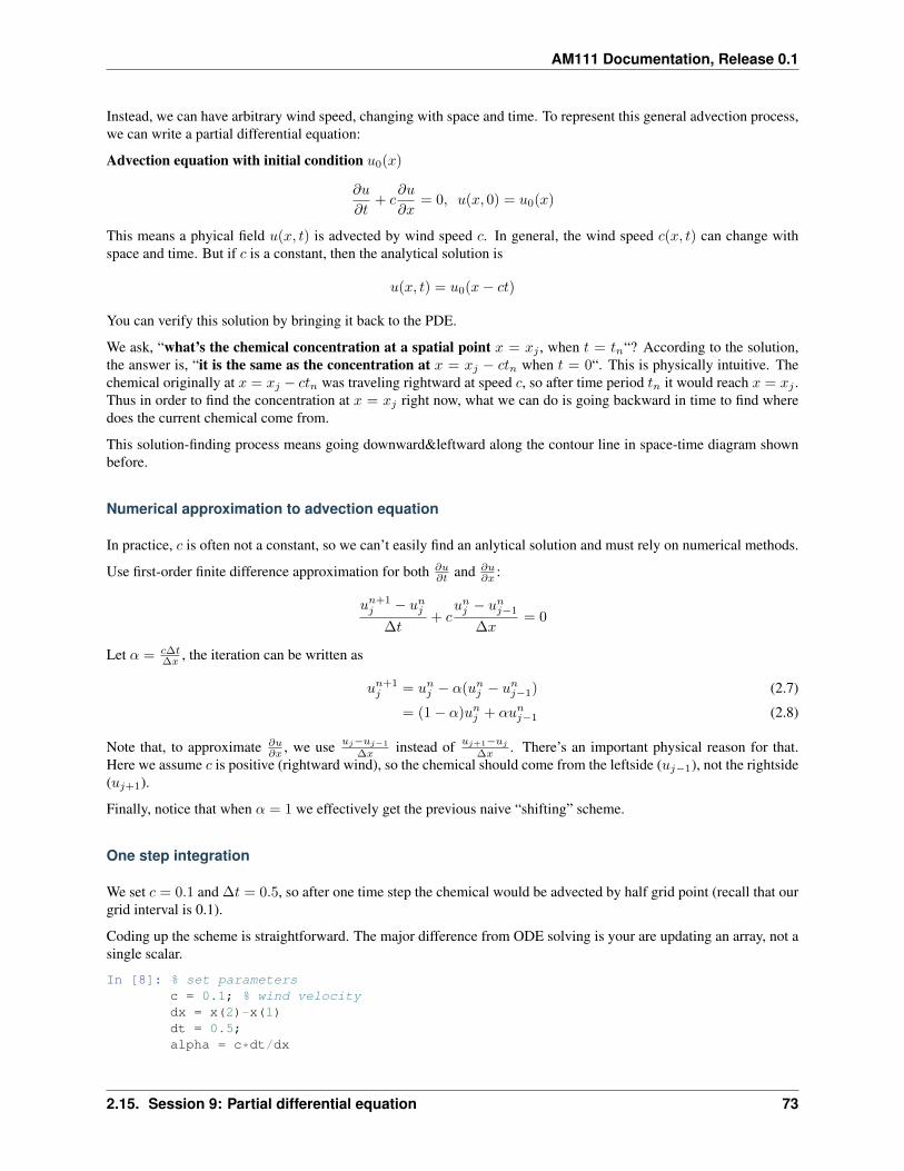
AM111 Documentation, Release 0.1
Instead, we can have arbitrary wind speed, changing with space and time. To represent this general advection process,we can write a partial differential equation:
Advection equation with initial condition 𝑢0(𝑥)
𝜕𝑢
𝜕𝑡+ 𝑐
𝜕𝑢
𝜕𝑥= 0, 𝑢(𝑥, 0) = 𝑢0(𝑥)
This means a phyical field 𝑢(𝑥, 𝑡) is advected by wind speed 𝑐. In general, the wind speed 𝑐(𝑥, 𝑡) can change withspace and time. But if 𝑐 is a constant, then the analytical solution is
𝑢(𝑥, 𝑡) = 𝑢0(𝑥− 𝑐𝑡)
You can verify this solution by bringing it back to the PDE.
We ask, “what’s the chemical concentration at a spatial point 𝑥 = 𝑥𝑗 , when 𝑡 = 𝑡𝑛“? According to the solution,the answer is, “it is the same as the concentration at 𝑥 = 𝑥𝑗 − 𝑐𝑡𝑛 when 𝑡 = 0“. This is physically intuitive. Thechemical originally at 𝑥 = 𝑥𝑗 − 𝑐𝑡𝑛 was traveling rightward at speed 𝑐, so after time period 𝑡𝑛 it would reach 𝑥 = 𝑥𝑗 .Thus in order to find the concentration at 𝑥 = 𝑥𝑗 right now, what we can do is going backward in time to find wheredoes the current chemical come from.
This solution-finding process means going downward&leftward along the contour line in space-time diagram shownbefore.
Numerical approximation to advection equation
In practice, 𝑐 is often not a constant, so we can’t easily find an anlytical solution and must rely on numerical methods.
Use first-order finite difference approximation for both 𝜕𝑢𝜕𝑡 and 𝜕𝑢
𝜕𝑥 :
𝑢𝑛+1𝑗 − 𝑢𝑛
𝑗
∆𝑡+ 𝑐
𝑢𝑛𝑗 − 𝑢𝑛
𝑗−1
∆𝑥= 0
Let 𝛼 = 𝑐Δ𝑡Δ𝑥 , the iteration can be written as
𝑢𝑛+1𝑗 = 𝑢𝑛
𝑗 − 𝛼(𝑢𝑛𝑗 − 𝑢𝑛
𝑗−1) (2.7)
= (1 − 𝛼)𝑢𝑛𝑗 + 𝛼𝑢𝑛
𝑗−1 (2.8)
Note that, to approximate 𝜕𝑢𝜕𝑥 , we use 𝑢𝑗−𝑢𝑗−1
Δ𝑥 instead of 𝑢𝑗+1−𝑢𝑗
Δ𝑥 . There’s an important physical reason for that.Here we assume 𝑐 is positive (rightward wind), so the chemical should come from the leftside (𝑢𝑗−1), not the rightside(𝑢𝑗+1).
Finally, notice that when 𝛼 = 1 we effectively get the previous naive “shifting” scheme.
One step integration
We set 𝑐 = 0.1 and ∆𝑡 = 0.5, so after one time step the chemical would be advected by half grid point (recall that ourgrid interval is 0.1).
Coding up the scheme is straightforward. The major difference from ODE solving is your are updating an array, not asingle scalar.
In [8]: % set parametersc = 0.1; % wind velocitydx = x(2)-x(1)dt = 0.5;alpha = c*dt/dx
2.15. Session 9: Partial differential equation 73
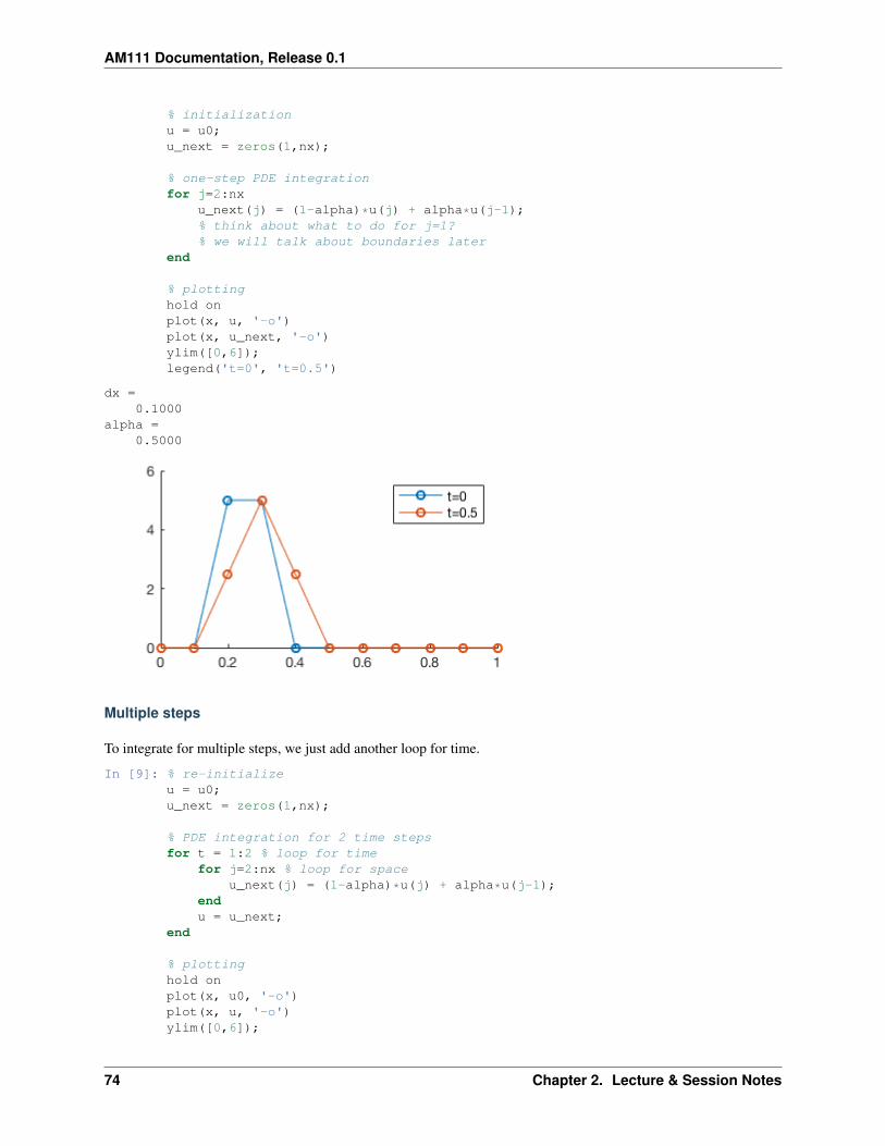
AM111 Documentation, Release 0.1
% initializationu = u0;u_next = zeros(1,nx);
% one-step PDE integrationfor j=2:nx
u_next(j) = (1-alpha)*u(j) + alpha*u(j-1);% think about what to do for j=1?% we will talk about boundaries later
end
% plottinghold onplot(x, u, '-o')plot(x, u_next, '-o')ylim([0,6]);legend('t=0', 't=0.5')
dx =0.1000
alpha =0.5000
Multiple steps
To integrate for multiple steps, we just add another loop for time.
In [9]: % re-initializeu = u0;u_next = zeros(1,nx);
% PDE integration for 2 time stepsfor t = 1:2 % loop for time
for j=2:nx % loop for spaceu_next(j) = (1-alpha)*u(j) + alpha*u(j-1);
endu = u_next;
end
% plottinghold onplot(x, u0, '-o')plot(x, u, '-o')ylim([0,6]);
74 Chapter 2. Lecture & Session Notes
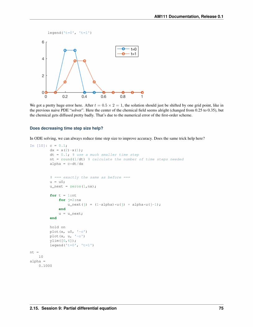
AM111 Documentation, Release 0.1
legend('t=0', 't=1')
We got a pretty huge error here. After 𝑡 = 0.5 × 2 = 1, the solution should just be shifted by one grid point, like inthe previous naive PDE “solver”. Here the center of the chemical field seems alright (changed from 0.25 to 0.35), butthe chemical gets diffused pretty badly. That’s due to the numerical error of the first-order scheme.
Does decreasing time step size help?
In ODE solving, we can always reduce time step size to improve accuracy. Does the same trick help here?
In [10]: c = 0.1;dx = x(2)-x(1);dt = 0.1; % use a much smaller time stepnt = round(1/dt) % calculate the number of time steps neededalpha = c*dt/dx
% === exactly the same as before ===u = u0;u_next = zeros(1,nx);
for t = 1:ntfor j=2:nx
u_next(j) = (1-alpha)*u(j) + alpha*u(j-1);endu = u_next;
end
hold onplot(x, u0, '-o')plot(x, u, '-o')ylim([0,6]);legend('t=0', 't=1')
nt =10
alpha =0.1000
2.15. Session 9: Partial differential equation 75
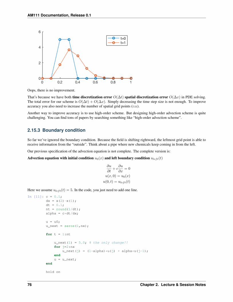
AM111 Documentation, Release 0.1
Oops, there is no improvement.
That’s because we have both time discretization error 𝑂(∆𝑡) spatial discretization error 𝑂(∆𝑥) in PDE solving.The total error for our scheme is 𝑂(∆𝑡) + 𝑂(∆𝑥). Simply decreasing the time step size is not enough. To improveaccuracy you also need to increase the number of spatial grid points (nx).
Another way to improve accuracy is to use high-order scheme. But designing high-order advection scheme is quitechallenging. You can find tons of papers by searching something like “high-order advection scheme”.
2.15.3 Boundary condition
So far we’ve ignored the boundary condition. Because the field is shifting rightward, the leftmost grid point is able toreceive information from the “outside”. Think about a pipe where new chemicals keep coming in from the left.
Our previous specification of the advection equation is not complete. The complete version is:
Advection equation with initial condition 𝑢0(𝑥) and left boundary condition 𝑢𝑙𝑒𝑓𝑡(𝑡)
𝜕𝑢
𝜕𝑡+ 𝑐
𝜕𝑢
𝜕𝑥= 0
𝑢(𝑥, 0) = 𝑢0(𝑥)
𝑢(0, 𝑡) = 𝑢𝑙𝑒𝑓𝑡(𝑡)
Here we assume 𝑢𝑙𝑒𝑓𝑡(𝑡) = 5. In the code, you just need to add one line.
In [11]: c = 0.1;dx = x(2)-x(1);dt = 0.1;nt = round(1/dt);alpha = c*dt/dx;
u = u0;u_next = zeros(1,nx);
for t = 1:nt
u_next(1) = 5.0; % the only change!!for j=2:nx
u_next(j) = (1-alpha)*u(j) + alpha*u(j-1);endu = u_next;
end
hold on
76 Chapter 2. Lecture & Session Notes
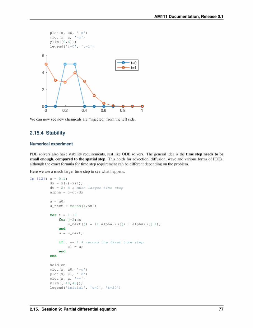
AM111 Documentation, Release 0.1
plot(x, u0, '-o')plot(x, u, '-o')ylim([0,6]);legend('t=0', 't=1')
We can now see new chemicals are “injected” from the left side.
2.15.4 Stability
Numerical experiment
PDE solvers also have stability requirements, just like ODE solvers. The general idea is the time step needs to besmall enough, compared to the spatial step. This holds for advection, diffusion, wave and various forms of PDEs,although the exact formula for time step requirement can be different depending on the problem.
Here we use a much larger time step to see what happens.
In [12]: c = 0.1;dx = x(2)-x(1);dt = 2; % a much larger time stepalpha = c*dt/dx
u = u0;u_next = zeros(1,nx);
for t = 1:10for j=2:nx
u_next(j) = (1-alpha)*u(j) + alpha*u(j-1);endu = u_next;
if t == 1 % record the first time stepu1 = u;
endend
hold onplot(x, u0, '-o')plot(x, u1, '-o')plot(x, u, '--')ylim([-40,40]);legend('initial', 't=2', 't=20')
2.15. Session 9: Partial differential equation 77
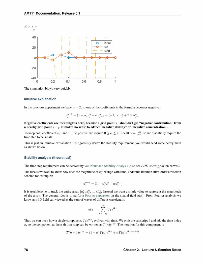
AM111 Documentation, Release 0.1
alpha =2
The simulation blows very quickly.
Intuitive explanation
In the previous experiment we have 𝛼 = 2, so one of the coeffcients in the formula becomes negative:
𝑢𝑛+1𝑗 = (1 − 𝛼)𝑢𝑛
𝑗 + 𝛼𝑢𝑛𝑗−1 = (−1) × 𝑢𝑛
𝑗 + 2 × 𝑢𝑛𝑗−1
Negative coefficients are meaningless here, because a grid point 𝑥𝑗 shouldn’t get “negative contribution” froma nearby grid point 𝑥𝑗−1. It makes no sense to advect “negative density” or “negative concentration”.
To keep both coefficients (𝛼 and 1 − 𝛼) postive, we require 0 ≤ 𝛼 ≤ 1. Recall 𝛼 = 𝑐Δ𝑡Δ𝑥 , so we essentially require the
time step to be small.
This is just an intuitive explanation. To rigorously derive the stability requirement, you would need some heavy mathas shown below.
Stability analysis (theoretical)
The time step requirement can be derived by von Neumann Stability Analysis (also see PDE_solving.pdf on canvas).
The idea is we want to know how does the magnitude of 𝑢𝑛𝑗 change with time, under the iteration (first-order advection
scheme for example):
𝑢𝑛+1𝑗 = (1 − 𝛼)𝑢𝑛
𝑗 + 𝛼𝑢𝑛𝑗−1
It is troublesome to track the entire array [𝑢𝑛1 , 𝑢
𝑛2 , ..., 𝑢
𝑛𝑚]. Instead we want a single value to represent the magnitude
of the array. The general idea is to perform Fourier expansion on the spatial field 𝑢(𝑥). From Fourier analysis weknow any 1D field can viewed as the sum of waves of different wavelength:
𝑢(𝑥) =
∞∑𝑘=−∞
𝑇𝑘𝑒𝑖𝑘𝑥
Thus we can track how a single component, 𝑇𝑘𝑒𝑖𝑘𝑥, evolves with time. We omit the subscript 𝑘 and add the time index
𝑛, so the component at the n-th time step can be written as 𝑇 (𝑛)𝑒𝑖𝑘𝑥. The iteration for this component is
𝑇 (𝑛 + 1)𝑒𝑖𝑘𝑥 = (1 − 𝛼)𝑇 (𝑛)𝑒𝑖𝑘𝑥 + 𝛼𝑇 (𝑛)𝑒𝑖𝑘(𝑥−Δ𝑥)
78 Chapter 2. Lecture & Session Notes

AM111 Documentation, Release 0.1
Divide both sides by 𝑒𝑖𝑘𝑥
𝑇 (𝑛 + 1) = (1 − 𝛼)𝑇 (𝑛) + 𝛼𝑇 (𝑛)𝑒−𝑖𝑘Δ𝑥
𝑇 (𝑛 + 1)
𝑇 (𝑛)= 1 − 𝛼 + 𝛼𝑒−𝑖𝑘Δ𝑥
Define amplification factor 𝐴 = 𝑇 (𝑛+1)𝑇 (𝑛) . We want |𝐴| ≤ 1 so the solution won’t blow up, just like what we did in
the ODE stability analysis.
We thus require
|1 − 𝛼 + 𝛼𝑒−𝑖𝑘Δ𝑥| ≤ 1
So we’ve transformed the requirement on an array to the requirement on a scalar.
We want this inequality to be true for any 𝑘. It will finally lead to a requirement for 𝛼, which is the same as theprevious intuitive analysis that 0 ≤ 𝛼 ≤ 1. Fully working this out needs some math, see this post for example.
2.15.5 High-order PDE
The wave equation is a typical 2nd-order PDE
𝜕2𝑢
𝜕𝑡2− 𝑐2
𝜕2𝑢
𝜕𝑥2= 0
Compared to the advection equation, the major differences are
• The wave can go both rightward and leftward, at speed 𝑐 or −𝑐.
• It needs both left and right boundary condition. Periodic boundary conditions are often used.
• It needs both 0th-order and 1st-order initial conditions, i.e. 𝑢(𝑥, 𝑡)|𝑡=0 and 𝜕𝑢𝜕𝑡 |𝑡=0. Otherwise you can’t start
your intergration, because a 2nd-order time derivative means 𝑢𝑛+1 would rely on both 𝑢𝑛 and 𝑢𝑛−1. 0th-orderinitial condition only gives you one time step, but you need two time steps to get started.
2.16 Session 10: Fast Fourier Transform
Date: 11/27/2017, Monday
In [1]: format compact
2.16.1 Generate input signal
Fourier transform is widely used in signal processing. Let’s looks at the simplest cosine signal first.
Define
𝑦1(𝑡) = 0.3 + 0.7 cos(2𝜋𝑓1𝑡)
It has a magnitude of 0.7, with a constant bias term 0.3. We choose the frequency 𝑓1 = 0.5.
In [2]: t = -5:0.1:4.9; % time axisN = length(t) % size of the signal
f1 = 0.5; % signal frequencyy1 = 0.3 + 0.7*cos(2*pi*f1*t); % the signal
2.16. Session 10: Fast Fourier Transform 79
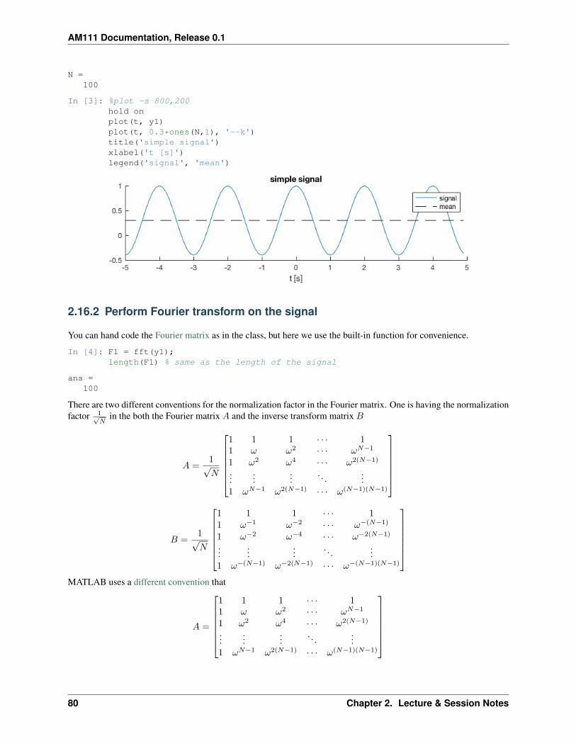
AM111 Documentation, Release 0.1
N =100
In [3]: %plot -s 800,200hold onplot(t, y1)plot(t, 0.3*ones(N,1), '--k')title('simple signal')xlabel('t [s]')legend('signal', 'mean')
2.16.2 Perform Fourier transform on the signal
You can hand code the Fourier matrix as in the class, but here we use the built-in function for convenience.
In [4]: F1 = fft(y1);length(F1) % same as the length of the signal
ans =100
There are two different conventions for the normalization factor in the Fourier matrix. One is having the normalizationfactor 1√
𝑁in the both the Fourier matrix 𝐴 and the inverse transform matrix 𝐵
𝐴 =1√𝑁
⎡⎢⎢⎢⎢⎢⎣1 1 1 · · · 11 𝜔 𝜔2 · · · 𝜔𝑁−1
1 𝜔2 𝜔4 · · · 𝜔2(𝑁−1)
......
.... . .
...1 𝜔𝑁−1 𝜔2(𝑁−1) · · · 𝜔(𝑁−1)(𝑁−1)
⎤⎥⎥⎥⎥⎥⎦
𝐵 =1√𝑁
⎡⎢⎢⎢⎢⎢⎣1 1 1 · · · 11 𝜔−1 𝜔−2 · · · 𝜔−(𝑁−1)
1 𝜔−2 𝜔−4 · · · 𝜔−2(𝑁−1)
......
.... . .
...1 𝜔−(𝑁−1) 𝜔−2(𝑁−1) · · · 𝜔−(𝑁−1)(𝑁−1)
⎤⎥⎥⎥⎥⎥⎦MATLAB uses a different convention that
𝐴 =
⎡⎢⎢⎢⎢⎢⎣1 1 1 · · · 11 𝜔 𝜔2 · · · 𝜔𝑁−1
1 𝜔2 𝜔4 · · · 𝜔2(𝑁−1)
......
.... . .
...1 𝜔𝑁−1 𝜔2(𝑁−1) · · · 𝜔(𝑁−1)(𝑁−1)
⎤⎥⎥⎥⎥⎥⎦
80 Chapter 2. Lecture & Session Notes
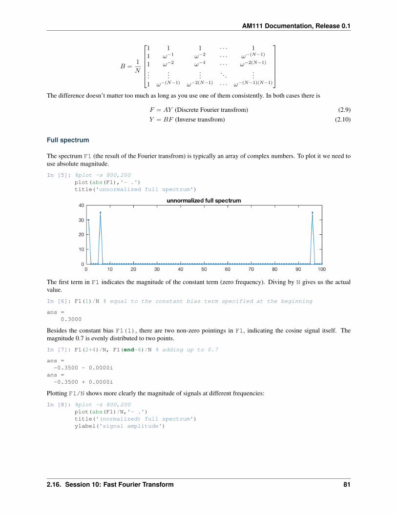
AM111 Documentation, Release 0.1
𝐵 =1
𝑁
⎡⎢⎢⎢⎢⎢⎣1 1 1 · · · 11 𝜔−1 𝜔−2 · · · 𝜔−(𝑁−1)
1 𝜔−2 𝜔−4 · · · 𝜔−2(𝑁−1)
......
.... . .
...1 𝜔−(𝑁−1) 𝜔−2(𝑁−1) · · · 𝜔−(𝑁−1)(𝑁−1)
⎤⎥⎥⎥⎥⎥⎦The difference doesn’t matter too much as long as you use one of them consistently. In both cases there is
𝐹 = 𝐴𝑌 (Discrete Fourier transfrom) (2.9)𝑌 = 𝐵𝐹 (Inverse transfrom) (2.10)
Full spectrum
The spectrum F1 (the result of the Fourier transfrom) is typically an array of complex numbers. To plot it we need touse absolute magnitude.
In [5]: %plot -s 800,200plot(abs(F1),'- .')title('unnormalized full spectrum')
The first term in F1 indicates the magnitude of the constant term (zero frequency). Diving by N gives us the actualvalue.
In [6]: F1(1)/N % equal to the constant bias term specified at the beginning
ans =0.3000
Besides the constant bias F1(1), there are two non-zero pointings in F1, indicating the cosine signal itself. Themagnitude 0.7 is evenly distributed to two points.
In [7]: F1(2+4)/N, F1(end-4)/N % adding up to 0.7
ans =-0.3500 - 0.0000i
ans =-0.3500 + 0.0000i
Plotting F1/N shows more clearly the magnitude of signals at different frequencies:
In [8]: %plot -s 800,200plot(abs(F1)/N,'- .')title('(normalized) full spectrum')ylabel('signal amplitude')
2.16. Session 10: Fast Fourier Transform 81
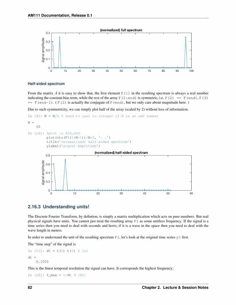
AM111 Documentation, Release 0.1
Half-sided spectrum
From the matrix 𝐴 it is easy to show that, the first element F(1) in the resulting spectrum is always a real numberindicating the constant bias term, while the rest of the array F(2:end) is symmetric, i.e. F(2) == F(end), F(3)== F(end-1). ( F(2) is actually the conjugate of F(end), but we only care about magnitude here. )
Due to such symmetricity, we can simply plot half of the array (scaled by 2) without loss of information.
In [9]: M = N/2 % need to cast to integer if N is an odd number
M =50
In [10]: %plot -s 800,200plot(abs(F1(1:M+1))/N*2, '- .')title('(normalized) half-sided spectrum')ylabel('signal amplitude')
2.16.3 Understanding units!
The Discrete Fourier Transform, by defintion, is simply a matrix multiplication which acts on pure numbers. But realphysical signals have units. You cannot just treat the resulting array F1 as some unitless frequency. If the signal is atime series then you need to deal with seconds and hertz; if it is a wave in the space then you need to deal with thewave length in meters.
In order to understand the unit of the resulting spectrum F1, let’s look at the original time series y1 first.
The “time step” of the signal is
In [11]: dt = t(2)-t(1) % [s]
dt =0.1000
This is the finest temporal resolution the signal can have. It corresponds the highest frequency:
In [12]: f_max = 1/dt % [Hz]
82 Chapter 2. Lecture & Session Notes
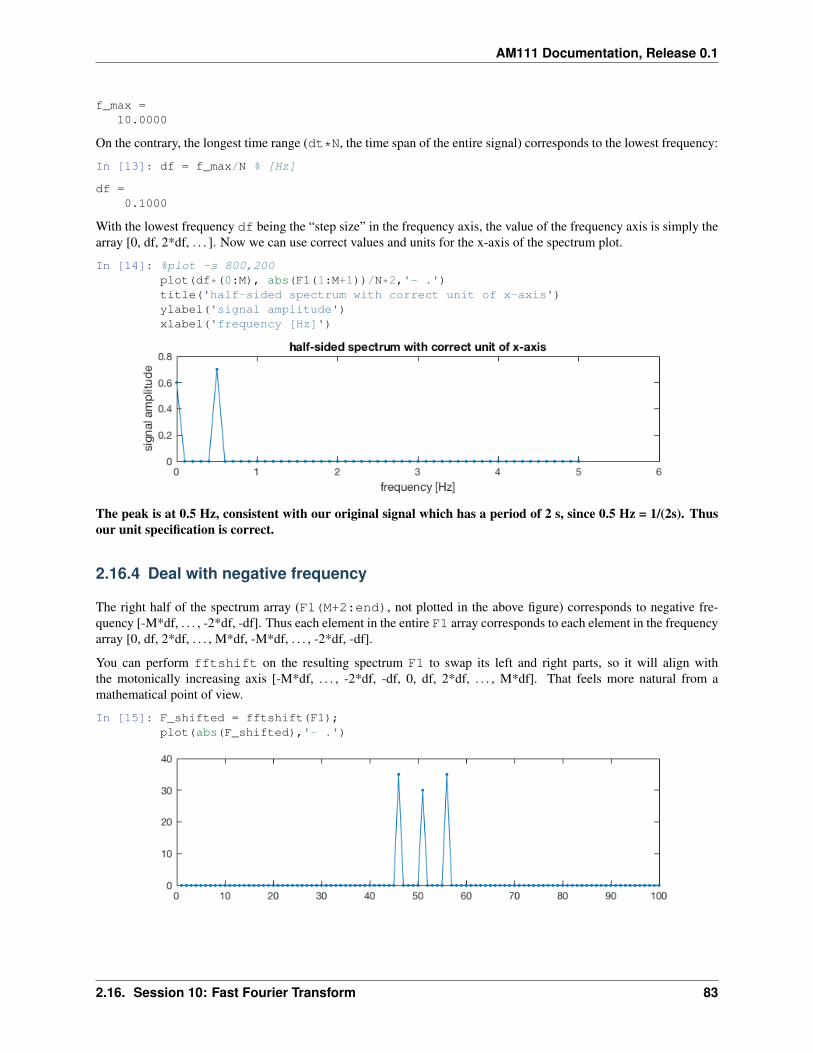
AM111 Documentation, Release 0.1
f_max =10.0000
On the contrary, the longest time range (dt*N, the time span of the entire signal) corresponds to the lowest frequency:
In [13]: df = f_max/N % [Hz]
df =0.1000
With the lowest frequency df being the “step size” in the frequency axis, the value of the frequency axis is simply thearray [0, df, 2*df, . . . ]. Now we can use correct values and units for the x-axis of the spectrum plot.
In [14]: %plot -s 800,200plot(df*(0:M), abs(F1(1:M+1))/N*2,'- .')title('half-sided spectrum with correct unit of x-axis')ylabel('signal amplitude')xlabel('frequency [Hz]')
The peak is at 0.5 Hz, consistent with our original signal which has a period of 2 s, since 0.5 Hz = 1/(2s). Thusour unit specification is correct.
2.16.4 Deal with negative frequency
The right half of the spectrum array (F1(M+2:end), not plotted in the above figure) corresponds to negative fre-quency [-M*df, . . . , -2*df, -df]. Thus each element in the entire F1 array corresponds to each element in the frequencyarray [0, df, 2*df, . . . , M*df, -M*df, . . . , -2*df, -df].
You can perform fftshift on the resulting spectrum F1 to swap its left and right parts, so it will align withthe motonically increasing axis [-M*df, . . . , -2*df, -df, 0, df, 2*df, . . . , M*df]. That feels more natural from amathematical point of view.
In [15]: F_shifted = fftshift(F1);plot(abs(F_shifted),'- .')
2.16. Session 10: Fast Fourier Transform 83
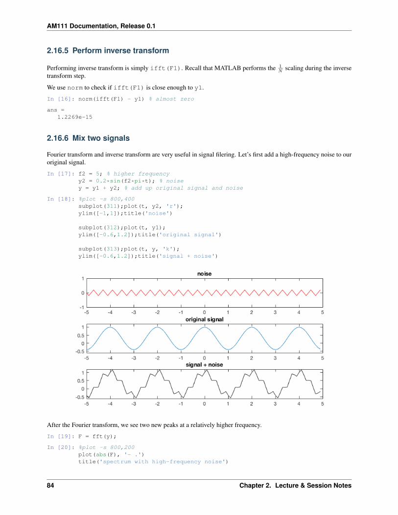
AM111 Documentation, Release 0.1
2.16.5 Perform inverse transform
Performing inverse transform is simply ifft(F1). Recall that MATLAB performs the 1𝑁 scaling during the inverse
transform step.
We use norm to check if ifft(F1) is close enough to y1.
In [16]: norm(ifft(F1) - y1) % almost zero
ans =1.2269e-15
2.16.6 Mix two signals
Fourier transform and inverse transform are very useful in signal filering. Let’s first add a high-frequency noise to ouroriginal signal.
In [17]: f2 = 5; % higher frequencyy2 = 0.2*sin(f2*pi*t); % noisey = y1 + y2; % add up original signal and noise
In [18]: %plot -s 800,400subplot(311);plot(t, y2, 'r');ylim([-1,1]);title('noise')
subplot(312);plot(t, y1);ylim([-0.6,1.2]);title('original signal')
subplot(313);plot(t, y, 'k');ylim([-0.6,1.2]);title('signal + noise')
After the Fourier transform, we see two new peaks at a relatively higher frequency.
In [19]: F = fft(y);
In [20]: %plot -s 800,200plot(abs(F), '- .')title('spectrum with high-frequency noise')
84 Chapter 2. Lecture & Session Notes
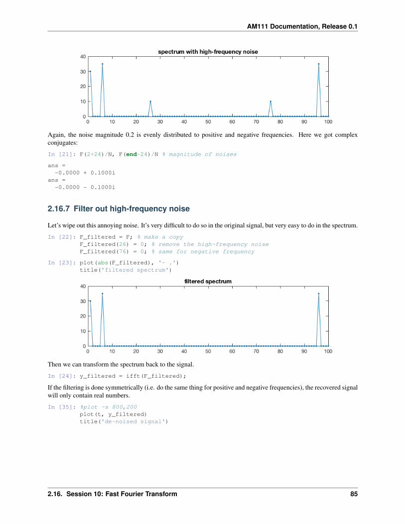
AM111 Documentation, Release 0.1
Again, the noise magnitude 0.2 is evenly distributed to positive and negative frequencies. Here we got complexconjugates:
In [21]: F(2+24)/N, F(end-24)/N % magnitude of noises
ans =-0.0000 + 0.1000i
ans =-0.0000 - 0.1000i
2.16.7 Filter out high-frequency noise
Let’s wipe out this annoying noise. It’s very difficult to do so in the original signal, but very easy to do in the spectrum.
In [22]: F_filtered = F; % make a copyF_filtered(26) = 0; % remove the high-frequency noiseF_filtered(76) = 0; % same for negative frequency
In [23]: plot(abs(F_filtered), '- .')title('filtered spectrum')
Then we can transform the spectrum back to the signal.
In [24]: y_filtered = ifft(F_filtered);
If the filtering is done symmetrically (i.e. do the same thing for positive and negative frequencies), the recovered signalwill only contain real numbers.
In [35]: %plot -s 800,200plot(t, y_filtered)title('de-noised signal')
2.16. Session 10: Fast Fourier Transform 85
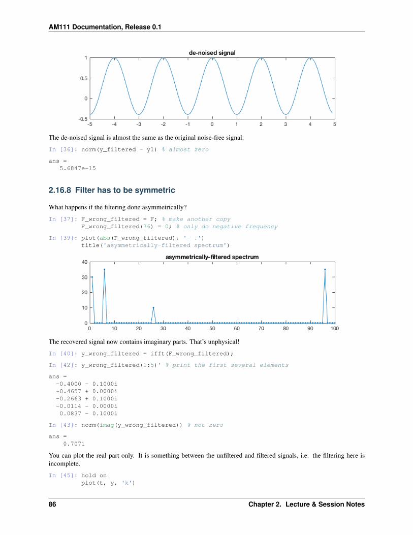
AM111 Documentation, Release 0.1
The de-noised signal is almost the same as the original noise-free signal:
In [36]: norm(y_filtered - y1) % almost zero
ans =5.6847e-15
2.16.8 Filter has to be symmetric
What happens if the filtering done asymmetrically?
In [37]: F_wrong_filtered = F; % make another copyF_wrong_filtered(76) = 0; % only do negative frequency
In [39]: plot(abs(F_wrong_filtered), '- .')title('asymmetrically-filtered spectrum')
The recovered signal now contains imaginary parts. That’s unphysical!
In [40]: y_wrong_filtered = ifft(F_wrong_filtered);
In [42]: y_wrong_filtered(1:5)' % print the first several elements
ans =-0.4000 - 0.1000i-0.4657 + 0.0000i-0.2663 + 0.1000i-0.0114 - 0.0000i0.0837 - 0.1000i
In [43]: norm(imag(y_wrong_filtered)) % not zero
ans =0.7071
You can plot the real part only. It is something between the unfiltered and filtered signals, i.e. the filtering here isincomplete.
In [45]: hold onplot(t, y, 'k')
86 Chapter 2. Lecture & Session Notes

AM111 Documentation, Release 0.1
plot(t, real(y_wrong_filtered), 'b')plot(t, y1, 'r')legend('signal with noise', 'incomplete fliltering', 'signal without noise')
These notes combine codes and results together. You can just copy the codes to your MATLAB console or script.
If you wonder how I wrote codes in this format and want to try it yourself, see the section below.
2.16. Session 10: Fast Fourier Transform 87

AM111 Documentation, Release 0.1
88 Chapter 2. Lecture & Session Notes
CHAPTER 3
MATLAB in Jupyter Notebooks
This course is taught in MATLAB. One thing you could try is to run MATLAB codes in Jupyter Notebooks. JupyterNotebook is a must-learn tool for data scientists, and it is also becoming popular in the traditional scientific computingcommunity. It is a great tool for interactive computing and allows you to combine codes, simulation results, anddescriptions such as latex equations in a single file.
See how to install and use it at:
3.1 Install Jupyter-MATLAB
Prerequisites
• We assume that you are comfortable with Linux command line. If not, checkout out Ryans’ tutorial for example.
• We also assume that you already have MATLAB installed and working. This tutorial is tested successfully withMATLAB R2017a on Mac/Linux/Windows.
3.1.1 Install the standard Jupyter-Python notebook
Jupyter relies on Python, so the first thing is to install Anaconda, a popular distribution of scientific Python. Experi-enced users prefer Miniconda to only install necessary packages, but the standard Anaconda is more convenient forbeginners, especially on Windows.
Once you have conda installed, you should test the standard IPython notebook. For example, in the notebook execute
In [1]: %%python# I am in a MATLAB kernel so need to add the above IPython magic to use the python kernel instead.# You can skip this magic in a standard python kernelprint('hello from Python')
hello from Python
89
AM111 Documentation, Release 0.1
3.1.2 On Mac/Linux
(1) Python-side configuration
Open the terminal, execute the following command to check your installation of anaconda and python:
which conda pip python
All of them should be inside anaconda’s directory “. . . /anaconda3/bin”
MATLAB R2017a only interfaces with Python3.5, so we need to create a new virtual environment:
conda create -vv -n jmatlab python=3.5 jupyter
Enter this Python environment. Stay in this environment when executing any terminal commands (pip, python,jupyter) for rest of this tutorial.
source activate jmatlab
Then, install the Matlab kernel for Jupyter.
pip install matlab_kernal
python -m matlab_kernel install
Check if the kernel is installed correctly
jupyter kernelspec list
You should see both Python and MATLAB.
(2) MATLAB-side configuration
Now we need to expose the MATLAB executable to Jupyter.
Find your MATLAB directory. On Mac it will be like “/Applications/MATLAB_R2017a.app”.
Go to the “extern/engines/python” subdirectory and install the Python engine.
cd “/Applications/MATLAB_R2017a.app/extern/engines/python”
python setup.py install
(3) Start Jupyter notebook
cd your_working_directory
jupyter notebook
Now you should see both Python and MATLAB options when launching a new notebook. Check if the MATLABkernel is working by:
In [2]: disp('hello from MATLAB')
hello from MATLAB
See Use MATLAB in Jupyter Notebooks for more usages.
90 Chapter 3. MATLAB in Jupyter Notebooks
AM111 Documentation, Release 0.1
3.1.3 On Windows
Windows is always tricker when it comes to configuring software, but all you need is basically translating Linuxcommands into Windows commands.
Commonly used Linux/Mac <-> Windows command mappings are:
• cd folder/subfolder <-> cd folder\subfolder (type e: to change the disk E)
• pwd <-> cd
• ls <-> dir
You might also need to set environment variables if commands like “python” and “conda” cannot be recognized. Addthe following directories to the PATH variable:
• path_to_Anaconda_dir\
• path_to_Anaconda_dir\Scripts\
All steps are exactly the same as in the Mac/Linux section. Windows is indeed a litte bit annoying, but it doesn’tprevent Jupyter+MATLAB from working. Please contact me if you have any troubles.
3.2 Use MATLAB in Jupyter Notebooks
Jupyter Notebook is a great tool for interactive computing. It allows you to combine codes, simulation results, anddescriptions such as latex equations in a single file. It works for many langueges including MATLAB, the choice ofthis class.
For installation, see Install Jupyter-MATLAB.
3.2.1 Jupyter basics
The most commonly used Jupyter commands are
• enter – (in command mode) enter edit mode
• shift+enter – (in edit mode) execute current cell
• esc – (in edit mode) enter command mode, so you can use arrow keys to move to other cells
• b – (in command mode) insert empty cell below
• x – (in command mode) cut current cell
• v – (in command mode) paste the cell you’ve cut
• esc+m/y – change current code cell to markdown cell / reverse
For all commands see “Help” - “Keyboard shortcuts” in the toolbar.
3.2.2 Printing formats
The default output format is “loose”, which takes a lot of space.
In [1]: format loosefor i=1:2
i+1end
3.2. Use MATLAB in Jupyter Notebooks 91
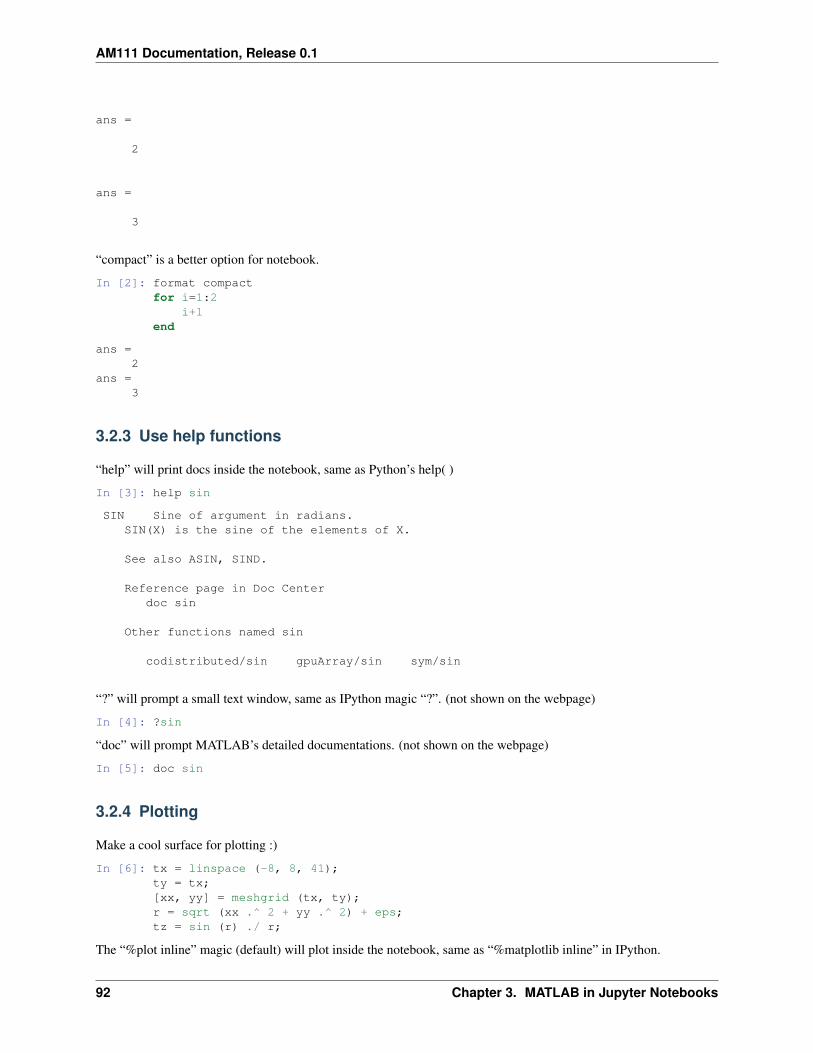
AM111 Documentation, Release 0.1
ans =
2
ans =
3
“compact” is a better option for notebook.
In [2]: format compactfor i=1:2
i+1end
ans =2
ans =3
3.2.3 Use help functions
“help” will print docs inside the notebook, same as Python’s help( )
In [3]: help sin
SIN Sine of argument in radians.SIN(X) is the sine of the elements of X.
See also ASIN, SIND.
Reference page in Doc Centerdoc sin
Other functions named sin
codistributed/sin gpuArray/sin sym/sin
“?” will prompt a small text window, same as IPython magic “?”. (not shown on the webpage)
In [4]: ?sin
“doc” will prompt MATLAB’s detailed documentations. (not shown on the webpage)
In [5]: doc sin
3.2.4 Plotting
Make a cool surface for plotting :)
In [6]: tx = linspace (-8, 8, 41);ty = tx;[xx, yy] = meshgrid (tx, ty);r = sqrt (xx .^ 2 + yy .^ 2) + eps;tz = sin (r) ./ r;
The “%plot inline” magic (default) will plot inside the notebook, same as “%matplotlib inline” in IPython.
92 Chapter 3. MATLAB in Jupyter Notebooks
AM111 Documentation, Release 0.1
In [7]: %plot inlinemesh(tx, ty, tz);
The “%plot native” magic will plot in an external window as the original MATLAB’s interface, which allows you torotate, zoom in/out (not shown on the webpage).
In [8]: %plot nativemesh(tx, ty, tz);
You can still use “close all” to close the window that was opened by cell above.
In [9]: close all
“?%plot” will show more plotting options including how to control the figure size (not shown on the webpage)
In [10]: ?%plot
3.2.5 User-defined functions
For Python programmers it is so common to define a custom function inside a notebook and reuse it over and overagain.
A ridiculous design of MATLAB is the function has to be in a separate file, with the function name being the file name.Local functions are allowed since R2016b, but it has many restrictions and doesn’t work in either Jupyter Notebookor MATLAB’s own Live Script.
Inline functions
By default, matlab only allows inline functions within a script.
3.2. Use MATLAB in Jupyter Notebooks 93
AM111 Documentation, Release 0.1
In [11]: f=@(x) x^3+x-1;
We can easily find the root of such a function.
In [12]: fzero(f,[0 1],optimset('Display','iter'))
Func-count x f(x) Procedure2 1 1 initial3 0.5 -0.375 bisection4 0.636364 -0.105935 interpolation5 0.68491 0.00620153 interpolation6 0.682225 -0.000246683 interpolation7 0.682328 -5.43508e-07 interpolation8 0.682328 1.50102e-13 interpolation9 0.682328 0 interpolation
Zero found in the interval [0, 1]ans =
0.6823
Standard functions
But inline functions must only contain a single statement, too limited in most cases.
If you try to define a standard function, it will fail:
In [13]: function p = multi_line_func(a,b)a = a+1;b = b+1;p = a+b;
end
Error: Function definitions are not permitted in this context.
Fortunately, Jupyter’s “%%file” magic allows us to write a code cell to a file.
In [14]: %%file multi_line_func.m
function p = multi_line_func(a,b)% in-file comments can be added like thisa = a+1;b = b+1;p = a+b;
end
Created file '/Users/zhuangjw/Research/Computing/personal_web/matlab_code/multi_line_func.m'.
The output file and this Notebook will be in the same directory, so you can call it directly, as if this function is definedinside the notebook.
In [15]: multi_line_func(1,1)
ans =4
By doing this, you get Python-like working environment – create a function, test it with several input parameters, goback to edit the function and test it again. This REPL workflow will greatly speed-up your prototyping.
It might take 1~2 seconds for a function cell to take effect, because we are writting files to disk. But you don’t needto restart the kernel to activate any modifications to your function.
94 Chapter 3. MATLAB in Jupyter Notebooks
AM111 Documentation, Release 0.1
warning: you should avoid adding a MATLAB comment (start with %) at the beginning of a cell, because it might beinterpreted as Jupyter magic and thus confuse the kernel.
3.2.6 Markdown cells
Markdown cells are a great way to add descriptions to your codes. Here are examples stolen from the official document.See Jupyter notebook’s document for details.
Latex equations
How to write an inline eqution: $e^i\pi + 1 = 0$
Result: 𝑒𝑖𝜋 + 1 = 0
How to write a standalone equation:
$$e^x=\sum_i=0^\infty \frac1i!x^i$$
Result:
𝑒𝑥 =
∞∑𝑖=0
1
𝑖!𝑥𝑖
Tables
How to make a table:
| This | is ||------|------|| a | table|
Result:
This isa table
Not-executing codes
You can put your codes inside a markdown cell, to only show the codes without executing them.
Here’s the way to get syntax highlighting for python codes:
```pythonpython codes```
“MATLAB” is not a highlighting option, but you can use “OCTAVE”, an open-source clone of MATLAB, to get thesame effect.
```OCTAVEdisp("Hello World")for i=1:2i+1
end```
3.2. Use MATLAB in Jupyter Notebooks 95
AM111 Documentation, Release 0.1
Result:
disp("Hello World")for i=1:2
i+1end
Headings
Headings are an important way to structure your notebook.
# Heading 1## Heading 2### Heading 3#### Heading 4
Some basic understanding of Linux command line and Python will be useful for installation. If you are just new toprogramming, you should simply use MATLAB’s original, basic user interface and come back to this tutoriallater when you are interested.
If you feel good about this tool, you can choose to submit notebooks for your homework, Again, your grade will notbe affected by the file format of your homework.
96 Chapter 3. MATLAB in Jupyter Notebooks


![AM111-01-40-Out [更新済み]...Title AM111-01-40-Out [更新済み].ai Author sakata Created Date 6/2/2011 2:38:22 PM](https://img.pdfslide.net/doc/110x75/60fa0fa1247dc9169c396b17/am111-01-40-out-title-am111-01-40-out-ai-author.jpg)