Embed Size (px)
Citation preview

AMELIA II: A Program for Missing Data
James Honaker, Gary King, and Matthew Blackwell
Version 1.7.5May 7, 2018
Contents
1 Introduction 3
2 What Amelia Does 32.1 Assumptions . . . . . . . . . . . . . . . . . . . . . . . . . . . . . . . . 42.2 Algorithm . . . . . . . . . . . . . . . . . . . . . . . . . . . . . . . . . 42.3 Analysis . . . . . . . . . . . . . . . . . . . . . . . . . . . . . . . . . . 5
3 Versions of Amelia 63.1 Installation and Updates from R . . . . . . . . . . . . . . . . . . . . . 73.2 Installation in Windows of AmeliaView as a Standalone Program . . 73.3 Linux (local installation) . . . . . . . . . . . . . . . . . . . . . . . . . 7
4 A User’s Guide 84.1 Data and Initial Results . . . . . . . . . . . . . . . . . . . . . . . . . 84.2 Multiple Imputation . . . . . . . . . . . . . . . . . . . . . . . . . . . 10
4.2.1 Saving imputed datasets . . . . . . . . . . . . . . . . . . . . . 114.2.2 Combining Multiple Amelia Runs . . . . . . . . . . . . . . . . 134.2.3 Screen Output . . . . . . . . . . . . . . . . . . . . . . . . . . . 15
4.3 Parallel Imputation Using Multicore CPUs . . . . . . . . . . . . . . . 164.4 Imputation-improving Transformations . . . . . . . . . . . . . . . . . 16
4.4.1 Ordinal . . . . . . . . . . . . . . . . . . . . . . . . . . . . . . 174.4.2 Nominal . . . . . . . . . . . . . . . . . . . . . . . . . . . . . . 184.4.3 Natural Log . . . . . . . . . . . . . . . . . . . . . . . . . . . . 194.4.4 Square Root . . . . . . . . . . . . . . . . . . . . . . . . . . . . 204.4.5 Logistic . . . . . . . . . . . . . . . . . . . . . . . . . . . . . . 20
4.5 Identification Variables . . . . . . . . . . . . . . . . . . . . . . . . . . 204.6 Time Series, or Time Series Cross Sectional Data . . . . . . . . . . . 21
4.6.1 Lags and Leads . . . . . . . . . . . . . . . . . . . . . . . . . . 224.7 Including Prior Information . . . . . . . . . . . . . . . . . . . . . . . 22
4.7.1 Ridge Priors for High Missingness, Small n’s, or Large Corre-lations . . . . . . . . . . . . . . . . . . . . . . . . . . . . . . . 22
4.7.2 Observation-level priors . . . . . . . . . . . . . . . . . . . . . 24
1

4.7.3 Logical bounds . . . . . . . . . . . . . . . . . . . . . . . . . . 274.8 Diagnostics . . . . . . . . . . . . . . . . . . . . . . . . . . . . . . . . 28
4.8.1 Comparing Densities . . . . . . . . . . . . . . . . . . . . . . . 284.8.2 Overimpute . . . . . . . . . . . . . . . . . . . . . . . . . . . . 294.8.3 Overdispersed Starting Values . . . . . . . . . . . . . . . . . . 344.8.4 Time-series plots . . . . . . . . . . . . . . . . . . . . . . . . . 344.8.5 Missingness maps . . . . . . . . . . . . . . . . . . . . . . . . . 37
4.9 Post-imputation Transformations . . . . . . . . . . . . . . . . . . . . 394.10 Analysis Models . . . . . . . . . . . . . . . . . . . . . . . . . . . . . . 404.11 The amelia class . . . . . . . . . . . . . . . . . . . . . . . . . . . . . 43
5 AmeliaView Menu Guide 455.1 Loading AmeliaView . . . . . . . . . . . . . . . . . . . . . . . . . . . 455.2 Loading a data set into AmeliaView . . . . . . . . . . . . . . . . . . . 455.3 Variable dashboard . . . . . . . . . . . . . . . . . . . . . . . . . . . . 455.4 Amelia Options . . . . . . . . . . . . . . . . . . . . . . . . . . . . . . 47
5.4.1 Numerical Options . . . . . . . . . . . . . . . . . . . . . . . . 495.4.2 Add Distribution Prior . . . . . . . . . . . . . . . . . . . . . . 505.4.3 Add Range Prior . . . . . . . . . . . . . . . . . . . . . . . . . 51
5.5 Imputing and checking diagnostics . . . . . . . . . . . . . . . . . . . 525.5.1 Diagnostics Dialog . . . . . . . . . . . . . . . . . . . . . . . . 52
5.6 Sessions . . . . . . . . . . . . . . . . . . . . . . . . . . . . . . . . . . 53
2

1 Introduction
Missing data is a ubiquitous problem in social science data. Respondents do notanswer every question, countries do not collect statistics every year, archives areincomplete, subjects drop out of panels. Most statistical analysis methods, however,assume the absence of missing data, and are only able to include observations forwhich every variable is measured. Amelia II allows users to impute (“fill in”or rectan-gularize) incomplete data sets so that analyses which require complete observationscan appropriately use all the information present in a dataset with missingness, andavoid the biases, inefficiencies, and incorrect uncertainty estimates that can resultfrom dropping all partially observed observations from the analysis.
Amelia II performs multiple imputation, a general-purpose approach to data withmissing values. Multiple imputation has been shown to reduce bias and increase ef-ficiency compared to listwise deletion. Furthermore, ad-hoc methods of imputation,such as mean imputation, can lead to serious biases in variances and covariances.Unfortunately, creating multiple imputations can be a burdensome process due tothe technical nature of algorithms involved. Amelia provides users with a simpleway to create and implement an imputation model, generate imputed datasets, andcheck its fit using diagnostics.
The Amelia II program goes several significant steps beyond the capabilities ofthe first version of Amelia (Honaker, Joseph, King, Scheve and Singh., 1998-2002).For one, the bootstrap-based EMB algorithm included in Amelia II can imputemany more variables, with many more observations, in much less time. The greatsimplicity and power of the EMB algorithm made it possible to write Amelia II sothat it virtually never crashes — which to our knowledge makes it unique amongall existing multiple imputation software — and is much faster than the alternativestoo. Amelia II also has features to make valid and much more accurate imputationsfor cross-sectional, time-series, and time-series-cross-section data, and allows theincorporation of observation and data-matrix-cell level prior information. In additionto all of this, Amelia II provides many diagnostic functions that help users check thevalidity of their imputation model. This software implements the ideas developed inHonaker and King (2010).
2 What Amelia Does
Multiple imputation involves imputing m values for each missing cell in your datamatrix and creating m “completed” data sets. Across these completed data sets, theobserved values are the same, but the missing values are filled in with a distribution ofimputations that reflect the uncertainty about the missing data. After imputationwith Amelia II’s EMB algorithm, you can apply whatever statistical method youwould have used if there had been no missing values to each of the m data sets,and use a simple procedure, described below, to combine the results1. Under normalcircumstances, you only need to impute once and can then analyze the m imputed
1You can combine the results automatically by doing your data analyses within Zelig for R, orwithin Clarify for Stata; see http://gking.harvard.edu/stats.shtml.
3

data sets as many times and for as many purposes as you wish. The advantage ofAmelia II is that it combines the comparative speed and ease-of-use of our algorithmwith the power of multiple imputation, to let you focus on your substantive researchquestions rather than spending time developing complex application-specific modelsfor nonresponse in each new data set. Unless the rate of missingness is very high,m = 5 (the program default) is probably adequate.
2.1 Assumptions
The imputation model in Amelia II assumes that the complete data (that is, bothobserved and unobserved) are multivariate normal. If we denote the (n× k) datasetas D (with observed part Dobs and unobserved part Dmis), then this assumption is
D ∼ Nk(µ,Σ), (1)
which states that D has a multivariate normal distribution with mean vector µ andcovariance matrix Σ. The multivariate normal distribution is often a crude approx-imation to the true distribution of the data, yet there is evidence that this modelworks as well as other, more complicated models even in the face of categorical ormixed data (see Schafer, 1997; Schafer and Olsen, 1998). Furthermore, transforma-tions of many types of variables can often make this normality assumption moreplausible (see 4.4 for more information on how to implement this in Amelia).
The essential problem of imputation is that we only observe Dobs, not the entiretyof D. In order to gain traction, we need to make the usual assumption in multipleimputation that the data are missing at random (MAR). This assumption meansthat the pattern of missingness only depends on the observed data Dobs, not theunobserved data Dmis. Let M to be the missingness matrix, with cells mij = 1 ifdij ∈ Dmis and mij = 0 otherwise. Put simply, M is a matrix that indicates whetheror not a cell is missing in the data. With this, we can define the MAR assumptionas
p(M |D) = p(M |Dobs). (2)
Note that MAR includes the case when missing values are created randomly by, say,coin flips, but it also includes many more sophisticated missingness models. Whenmissingness is not dependent on the data at all, we say that the data are missingcompletely at random (MCAR). Amelia requires both the multivariate normalityand the MAR assumption (or the simpler special case of MCAR). Note that theMAR assumption can be made more plausible by including additional variables inthe dataset D in the imputation dataset than just those eventually envisioned to beused in the analysis model.
2.2 Algorithm
In multiple imputation, we are concerned with the complete-data parameters, θ =(µ,Σ). When writing down a model of the data, it is clear that our observed data isactually Dobs and M , the missingness matrix. Thus, the likelihood of our observed
4

data is p(Dobs,M |θ). Using the MAR assumption2, we can break this up,
p(Dobs,M |θ) = p(M |Dobs)p(Dobs|θ). (3)
As we only care about inference on the complete data parameters, we can write thelikelihood as
L(θ|Dobs) ∝ p(Dobs|θ), (4)
which we can rewrite using the law of iterated expectations as
p(Dobs|θ) =
∫p(D|θ)dDmis. (5)
With this likelihood and a flat prior on θ, we can see that the posterior is
p(θ|Dobs) ∝ p(Dobs|θ) =
∫p(D|θ)dDmis. (6)
The main computational difficulty in the analysis of incomplete data is taking drawsfrom this posterior. The EM algorithm (Dempster, Laird and Rubin, 1977) is asimple computational approach to finding the mode of the posterior. Our EMB al-gorithm combines the classic EM algorithm with a bootstrap approach to take drawsfrom this posterior. For each draw, we bootstrap the data to simulate estimationuncertainty and then run the EM algorithm to find the mode of the posterior for thebootstrapped data, which gives us fundamental uncertainty too (see Honaker andKing (2010) for details of the EMB algorithm).
Once we have draws of the posterior of the complete-data parameters, we makeimputations by drawing values of Dmis from its distribution conditional on Dobs andthe draws of θ, which is a linear regression with parameters that can be calculateddirectly from θ.
2.3 Analysis
In order to combine the results across m data sets, first decide on the quantityof interest to compute, such as a univariate mean, regression coefficient, predictedprobability, or first difference. Then, the easiest way is to draw 1/m simulations of qfrom each of the m data sets, combine them into one set of m simulations, and thento use the standard simulation-based methods of interpretation common for singledata sets (King, Tomz and Wittenberg, 2000).
Alternatively, you can combine directly and use as the multiple imputation esti-mate of this parameter, q̄, the average of the m separate estimates, qj (j = 1, . . . ,m):
q̄ =1
m
m∑j=1
qj. (7)
2There is an additional assumption hidden here that M does not depend on the complete-dataparameters.
5

incomplete data?? ?
???
? ???
???
bootstrap
bootstrapped data
imputed datasetsEM
analysisseparate results
combination
final results
Figure 1: A schematic of our approach to multiple imputation with the EMB algo-rithm.
The variance of the point estimate is the average of the estimated variances fromwithin each completed data set, plus the sample variance in the point estimatesacross the data sets (multiplied by a factor that corrects for the bias because m <∞). Let SE(qj)
2 denote the estimated variance (squared standard error) of qj fromthe data set j, and S2
q = Σmj=1(qj − q̄)2/(m − 1) be the sample variance across the
m point estimates. The standard error of the multiple imputation point estimate isthe square root of
SE(q)2 =1
m
m∑j=1
SE(qj)2 + S2
q (1 + 1/m). (8)
3 Versions of Amelia
Two versions of Amelia II are available, each with its own advantages and drawbacks,but both of which use the same underlying code and algorithms. First, Amelia IIexists as a package for the R statistical software package. Users can utilize theirknowledge of the R language to run Amelia II at the command line or to create scriptsthat will run Amelia II and preserve the commands for future use. Alternatively, youmay prefer AmeliaView, where an interactive Graphical User Interface (GUI) allowsyou to set options and run Amelia without any knowledge of the R programminglanguage.
Both versions of Amelia II are available on the Windows, Mac OS X, and Linuxplatforms and Amelia II for R runs in any environment that R can. All versions ofAmelia require the R software, which is freely available at http://www.r-project.org/.
Before installing Amelia II, you must have installed R version 2.1.0 or higher,which is freely available at http://www.r-project.org/.
6

3.1 Installation and Updates from R
To install the Amelia package on any platform, simply type the following at the Rcommand prompt,
> install.packages("Amelia")
and R will automatically install the package to your system from CRAN. If you wishto use the most current beta version of Amelia feel free to install the test version,
> install.packages("Amelia", repos = "http://gking.harvard.edu")
In order to keep your copy of Amelia completely up to date, you should use thecommand
> update.packages()
3.2 Installation in Windows of AmeliaView as a StandaloneProgram
To install a standalone version of AmeliaView in the Windows environment, simplydownload the installer setup.exe from http://gking.harvard.edu/amelia/ andrun it. The installer will ask you to choose a location to install Amelia II. If youhave installed R with the default options, Amelia II will automatically find thelocation of R. If the installer cannot find R, it will ask you to locate the directoryof the most current version of R. Make sure you choose the directory name thatincludes the version number of R (e.g. C:/Program Files/R/R-2.9.0) and contains asubdirectory named bin. The installer will also put shortcuts on your Desktop andStart Menu.
Even users familiar with the R language may find it useful to utilize AmeliaViewto set options on variables, change arguments, or run diagnostics. From the com-mand line, AmeliaView can be brought up with the call:
> library(Amelia)
> AmeliaView()
3.3 Linux (local installation)
Installing Amelia on a Linux system is slightly more complicated due to user per-missions. If you are running R with root access, you can simply run the aboveinstallation procedure. If you do not have root access, you can install Amelia to alocal library. First, create a local directory to house the packages,
w4:mblackwell [~]: mkdir ~/myrlibrary
and then, in an R session, install the package directing R to this location:
> install.packages("Amelia", lib = "~/myrlibrary")
7

Once this is complete you need to edit or create your R profile. Locate or create~/.Rprofile in your home directory and add this line:
.libPath("~/myrlibrary")
This will add your local library to the list of library paths that R searches in whenyou load libraries.
Linux users can use AmeliaView in the same way as Windows users of Ameliafor R. From the command line, AmeliaView can be brought up with the call:
> AmeliaView()
4 A User’s Guide
4.1 Data and Initial Results
We now demonstrate how to use Amelia using data from Milner and Kubota (2005)which studies the effect of democracy on trade policy. For the purposes of this user’sguide, we will use a subset restricted to nine developing countries in Asia from1980 to 19993. This dataset includes 9 variables: year (year), country (country),average tariff rates (tariff), Polity IV score4 (polity), total population (pop), grossdomestic product per capita (gdp.pc), gross international reserves (intresmi), adummy variable signifying whether the country had signed an IMF agreement inthat year (signed), a measure of financial openness (fivop), and a measure of UShegemony5 (usheg). These variables correspond to the variables used in the analysismodel of Milner and Kubota (2005) in table 2.
We first load the Amelia and the data:
> require(Amelia)
> data(freetrade)
We can check the summary statistics of the data to see that there is missingnesson many of the variables:
> summary(freetrade)
year country tariff polity
Min. :1981 Length:171 Min. : 7.1 Min. :-8.0
1st Qu.:1985 Class :character 1st Qu.: 16.3 1st Qu.:-2.0
Median :1990 Mode :character Median : 25.2 Median : 5.0
Mean :1990 Mean : 31.6 Mean : 2.9
3rd Qu.:1995 3rd Qu.: 40.8 3rd Qu.: 8.0
3We have artificially added some missingness to these data for presentational purposes. Youcan access the original data at http://www.princeton.edu/~hmilner/Research.htm
4The Polity score is a number between -10 and 10 indicating how democratic a country is. Afully autocratic country would be a -10 while a fully democratic country would be 1 10.
5This measure of US hegemony is the US imports and exports as a percent of the world totalimports and exports.
8

Max. :1999 Max. :100.0 Max. : 9.0
NA's :58 NA's :2
pop gdp.pc intresmi signed
Min. :1.41e+07 Min. : 150 Min. :0.904 Min. :0.000
1st Qu.:1.97e+07 1st Qu.: 420 1st Qu.:2.223 1st Qu.:0.000
Median :5.28e+07 Median : 814 Median :3.182 Median :0.000
Mean :1.50e+08 Mean : 1867 Mean :3.375 Mean :0.155
3rd Qu.:1.21e+08 3rd Qu.: 2463 3rd Qu.:4.406 3rd Qu.:0.000
Max. :9.98e+08 Max. :12086 Max. :7.935 Max. :1.000
NA's :13 NA's :3
fiveop usheg
Min. :12.3 Min. :0.256
1st Qu.:12.5 1st Qu.:0.262
Median :12.6 Median :0.276
Mean :12.7 Mean :0.276
3rd Qu.:13.2 3rd Qu.:0.289
Max. :13.2 Max. :0.308
NA's :18
In the presence of missing data, most statistical packages use listwise deletion,which removes any row that contains a missing value from the analysis. Using thebase model of Milner and Kubota (2005) table 2, we run a simple linear model in R,which uses listwise deletion:
> summary(lm(tariff ~ polity + pop + gdp.pc + year + country,
+ data = freetrade))
Call:
lm(formula = tariff ~ polity + pop + gdp.pc + year + country,
data = freetrade)
Residuals:
Min 1Q Median 3Q Max
-30.764 -3.259 0.087 2.598 18.310
Coefficients:
Estimate Std. Error t value Pr(>|t|)
(Intercept) 1.97e+03 4.02e+02 4.91 3.6e-06
polity -1.37e-01 1.82e-01 -0.75 0.45
pop -2.02e-07 2.54e-08 -7.95 3.2e-12
gdp.pc 6.10e-04 7.44e-04 0.82 0.41
year -8.71e-01 2.08e-01 -4.18 6.4e-05
countryIndonesia -1.82e+02 1.86e+01 -9.82 3.0e-16
countryKorea -2.20e+02 2.08e+01 -10.61 < 2e-16
countryMalaysia -2.25e+02 2.17e+01 -10.34 < 2e-16
countryNepal -2.16e+02 2.25e+01 -9.63 7.7e-16
countryPakistan -1.55e+02 1.98e+01 -7.84 5.6e-12
9
countryPhilippines -2.04e+02 2.09e+01 -9.77 3.7e-16
countrySriLanka -2.09e+02 2.21e+01 -9.46 1.8e-15
countryThailand -1.96e+02 2.10e+01 -9.36 3.0e-15
Residual standard error: 6.22 on 98 degrees of freedom
(60 observations deleted due to missingness)
Multiple R-squared: 0.925, Adjusted R-squared: 0.915
F-statistic: 100 on 12 and 98 DF, p-value: <2e-16
Note that 60 of the 171 original observations are deleted due to missingness.These observations, however, are partially observed, and contain valuable informa-tion about the relationships between those variables which are present in the partiallycompleted observations. Multiple imputation will help us retrieve that informationand make better, more efficient, inferences.
4.2 Multiple Imputation
When performing multiple imputation, the first step is to identify the variables toinclude in the imputation model. It is crucial to include at least as much informationas will be used in the analysis model. That is, any variable that will be in the analysismodel should also be in the imputation model. This includes any transformationsor interactions of variables that will appear in the analysis model.
In fact, it is often useful to add more information to the imputation modelthan will be present when the analysis is run. Since imputation is predictive, anyvariables that would increase predictive power should be included in the model,even if including them in the analysis model would produce bias in estimating acausal effect (such as for post-treatment variables) or collinearity would precludedetermining which variable had a relationship with the dependent variable (suchas including multiple alternate measures of GDP). In our case, we include all thevariables in freetrade in the imputation model, even though our analysis modelfocuses on polity, pop and gdp.pc6.
To create multiple imputations in Amelia, we can simply run
> a.out <- amelia(freetrade, m = 5, ts = "year", cs = "country")
-- Imputation 1 --
1 2 3 4 5 6 7 8 9 10 11 12 13 14
-- Imputation 2 --
1 2 3 4 5 6 7 8 9 10 11 12 13 14 15
-- Imputation 3 --
6Note that this specification does not utilize time or spatial data yet. The ts and cs argumentsonly have force when we also include polytime or intercs, discussed in section 4.6
10
1 2 3 4 5 6 7 8 9
-- Imputation 4 --
1 2 3 4 5 6 7 8 9 10 11 12 13 14
-- Imputation 5 --
1 2 3 4 5 6 7 8 9 10
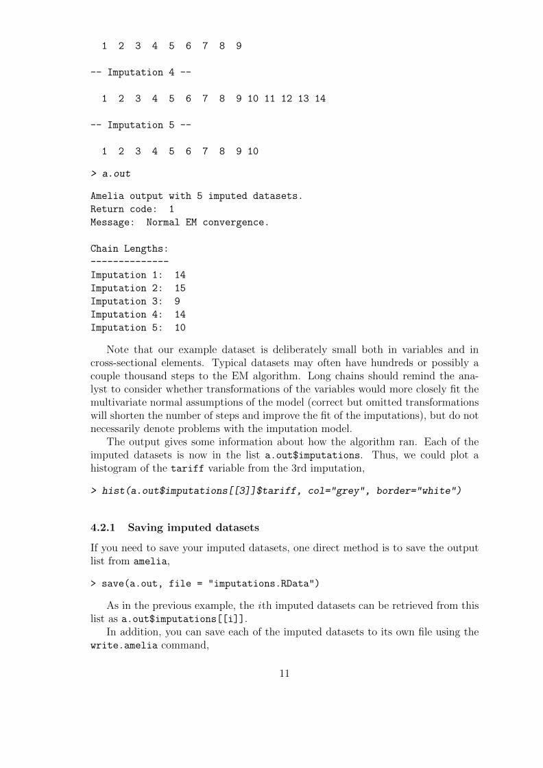
> a.out
Amelia output with 5 imputed datasets.
Return code: 1
Message: Normal EM convergence.
Chain Lengths:
--------------
Imputation 1: 14
Imputation 2: 15
Imputation 3: 9
Imputation 4: 14
Imputation 5: 10
Note that our example dataset is deliberately small both in variables and incross-sectional elements. Typical datasets may often have hundreds or possibly acouple thousand steps to the EM algorithm. Long chains should remind the ana-lyst to consider whether transformations of the variables would more closely fit themultivariate normal assumptions of the model (correct but omitted transformationswill shorten the number of steps and improve the fit of the imputations), but do notnecessarily denote problems with the imputation model.
The output gives some information about how the algorithm ran. Each of theimputed datasets is now in the list a.out$imputations. Thus, we could plot ahistogram of the tariff variable from the 3rd imputation,
> hist(a.out$imputations[[3]]$tariff, col="grey", border="white")
4.2.1 Saving imputed datasets
If you need to save your imputed datasets, one direct method is to save the outputlist from amelia,
> save(a.out, file = "imputations.RData")
As in the previous example, the ith imputed datasets can be retrieved from thislist as a.out$imputations[[i]].
In addition, you can save each of the imputed datasets to its own file using thewrite.amelia command,
11

Histogram of a.out$imputations[[3]]$tariff
a.out$imputations[[3]]$tariff
Fre
quen
cy
0 20 40 60 80 100
010
2030
40
Figure 2: Histogram of the tariff variable from the 3rd imputed dataset.
12

> write.amelia(obj=a.out, file.stem = "outdata")
This will create one comma-separated value file for each imputed dataset in thefollowing manner:
outdata1.csv
outdata2.csv
outdata3.csv
outdata4.csv
outdata5.csv
The write.amelia function can also save files in tab-delimited and Stata (.dta) fileformats. For instance, to save Stata files, simply change the format argument to"dta",
> write.amelia(obj=a.out, file.stem = "outdata", format = "dta")
Additionally, write.amelia can create a“stacked”version of the imputed datasetwhich stacks each imputed dataset on top of one another. This can be done by settingthe separate argument to FALSE. The resulting matrix is of size (N ·m)× p if theoriginal dataset is excluded (orig.data = FALSE) and of size (N · (m + 1)) × p ifit is included (orig.data = TRUE). The stacked dataset will include a variable(set with impvar) that indicates to which imputed dataset the observation belongs.See Section 4.10 for a description of how to use this stacked dataset with the mi
commands in Stata.
4.2.2 Combining Multiple Amelia Runs
The EMB algorithm is what computer scientists call embarrassingly parallel, meaningthat it is simple to separate each imputation into parallel processes. With Amelia itis simple to run subsets of the imputations on different machines and then combinethem after the imputation for use in analysis model. This allows for a huge increasein the speed of the algorithm.
Output lists from different Amelia runs can be combined together into a new list.For instance, suppose that we wanted to add another ten imputed datasets to ourearlier call to amelia. First, run the function to get these additional imputations,
> a.out.more <- amelia(freetrade, m = 10, ts = "year", cs = "country", p2s=0)
> a.out.more
Amelia output with 10 imputed datasets.
Return code: 1
Message: Normal EM convergence.
Chain Lengths:
--------------
Imputation 1: 12
Imputation 2: 13
13

Imputation 3: 13
Imputation 4: 14
Imputation 5: 17
Imputation 6: 15
Imputation 7: 15
Imputation 8: 15
Imputation 9: 15
Imputation 10: 19
then combine this output with our original output using the ameliabind function,
> a.out.more <- ameliabind(a.out, a.out.more)
> a.out.more
Amelia output with 15 imputed datasets.
Return code: 1
Message: Normal EM convergence
Chain Lengths:
--------------
Imputation 1: 14
Imputation 2: 15
Imputation 3: 9
Imputation 4: 14
Imputation 5: 10
Imputation 6: 12
Imputation 7: 13
Imputation 8: 13
Imputation 9: 14
Imputation 10: 17
Imputation 11: 15
Imputation 12: 15
Imputation 13: 15
Imputation 14: 15
Imputation 15: 19
This function binds the two outputs into the same output so that you can passthe combined imputations easily to analysis models and diagnostics. Note thata.out.more now has a total of 15 imputations.
A simple way to execute a parallel processing scheme with Amelia would be torun amelia with m set to 1 on m different machines or processors, save each outputusing the save function, load them all on the same R session using load commandand then combine them using ameliabind. In order to do this, however, make sureto name each of the outputs a different name so that they do not overwrite eachother when loading into the same R session. Also, some parallel environments willdump all generated files into a common directory, where they may overwrite eachother. If it is convenient in a parallel environment to run a large number of amelia
14
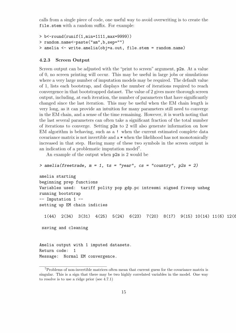
calls from a single piece of code, one useful way to avoid overwriting is to create thefile.stem with a random suffix. For example:
> b<-round(runif(1,min=1111,max=9999))
> random.name<-paste("am",b,sep="")
> amelia <- write.amelia(obj=a.out, file.stem = random.name)
4.2.3 Screen Output
Screen output can be adjusted with the “print to screen” argument, p2s. At a valueof 0, no screen printing will occur. This may be useful in large jobs or simulationswhere a very large number of imputation models may be required. The default valueof 1, lists each bootstrap, and displays the number of iterations required to reachconvergence in that bootstrapped dataset. The value of 2 gives more thorough screenoutput, including, at each iteration, the number of parameters that have significantlychanged since the last iteration. This may be useful when the EM chain length isvery long, as it can provide an intuition for many parameters still need to convergein the EM chain, and a sense of the time remaining. However, it is worth noting thatthe last several parameters can often take a significant fraction of the total numberof iterations to converge. Setting p2s to 2 will also generate information on howEM algorithm is behaving, such as a ! when the current estimated complete datacovariance matrix is not invertible and a * when the likelihood has not monotonicallyincreased in that step. Having many of these two symbols in the screen output isan indication of a problematic imputation model7.
An example of the output when p2s is 2 would be
> amelia(freetrade, m = 1, ts = "year", cs = "country", p2s = 2)
amelia starting
beginning prep functions
Variables used: tariff polity pop gdp.pc intresmi signed fiveop usheg
running bootstrap
-- Imputation 1 --
setting up EM chain indicies
1(44) 2(34) 3(31) 4(25) 5(24) 6(23) 7(20) 8(17) 9(15) 10(14) 11(6) 12(6) 13(4) 14(2) 15(0)
saving and cleaning
Amelia output with 1 imputed datasets.
Return code: 1
Message: Normal EM convergence.
7Problems of non-invertible matrices often mean that current guess for the covariance matrix issingular. This is a sign that there may be two highly correlated variables in the model. One wayto resolve is to use a ridge prior (see 4.7.1)
15

Chain Lengths:
--------------
Imputation 1: 15
4.3 Parallel Imputation Using Multicore CPUs
Each imputation in the above EMB algorithm is completely independent of anyother imputation, a property called embarrassingly parallel. This type of approachcan take advantage of the multiple -core infrastructure of modern CPUs. Each corein a multi-core processor can execute independent operations in parallel. Ameliacan utilize this parallel processing internally via the parallel and the ncpus ar-guments. The parallel argument sets the parallel processing backend, either with"multicore" or "snow" (or "no" for no parallel processing). The "multicore"
backend is not available on Windows systems, but tends to be quicker at parallelprocessing. On a Windows system, the "snow" backend provides parallel processingthrough a cluster of worker processes across the CPUs. You can set the default forthis argument using the "amelia.parallel" option. This allows you to run Ameliain parallel as the default for an entire R session without setting arguments in theamelia call.
For each of the parallel backends, Amelia requires a number of CPUs to use inparallel. This can be set using the ncpus argument. It can be higher than the numberof physical cores in the system if hyperthreading or other technologies are available.You can use the parallel::detectCores function to determine how many coresare available on your machine. The default for this argument can be set using the"amelia.ncpus" option.
On Unix-alike systems (such as Mac OS X and Linux distributions), the "multicore"backend automatically sets up and stops the parallel workers by forking the process.On Windows, the "snow" backend requires more attention. Amelia will attempt tocreate a parallel cluster of worker processes (since Windows systems cannot fork aprocess) and will stop this cluster after the imputations are complete. Alternatively,Amelia also has a cl argument, which accepts a predefined cluster made using theparallel::makePSOCKcluster. For more information about parallel processing inR, see the documentation for the parallel package that ships along with R.
4.4 Imputation-improving Transformations
Social science data commonly includes variables that fail to fit to a multivariatenormal distribution. Indeed, numerous models have been introduced specifically todeal with the problems they present. As it turns out, much evidence in the literature(discussed in King et al. 2001) indicates that the multivariate normal model usedin Amelia usually works well for the imputation stage even when discrete or non-normal variables are included and when the analysis stage involves these limiteddependent variable models. Nevertheless, Amelia includes some limited capacity todeal directly with ordinal and nominal variables and to modify variables that requireother transformations. In general nominal and log transform variables should bedeclared to Amelia, whereas ordinal (including dichotomous) variables often need
16

not be, as described below. (For harder cases, see (Schafer, 1997), for specializedMCMC-based imputation models for discrete variables.)
Although these transformations are taken internally on these variables to betterfit the data to the multivariate normal assumptions of the imputation model, all theimputations that are created will be returned in the original untransformed form ofthe data. If the user has already performed transformations on their data (such asby taking a log or square root prior to feeding the data to amelia) these do not needto be declared, as that would result in the transformation occurring doubly in theimputation model. The fully imputed data sets that are returned will always be inthe form of the original data that is passed to the amelia routine.
4.4.1 Ordinal
In much statistical research, researchers treat independent ordinal (including di-chotomous) variables as if they were really continuous. If the analysis model to beemployed is of this type, then nothing extra is required of the of the imputationmodel. Users are advised to allow Amelia to impute non-integer values for anymissing data, and to use these non-integer values in their analysis. Sometimes thismakes sense, and sometimes this defies intuition. One particular imputation of 2.35for a missing value on a seven point scale carries the intuition that the respondentis between a 2 and a 3 and most probably would have responded 2 had the databeen observed. This is easier to accept than an imputation of 0.79 for a dichotomousvariable where a zero represents a male and a one represents a female respondent.However, in both cases the non-integer imputations carry more information aboutthe underlying distribution than would be carried if we were to force the imputa-tions to be integers. Thus whenever the analysis model permits, missing ordinalobservations should be allowed to take on continuously valued imputations.
In the freetrade data, one such ordinal variable is polity which ranges from-10 (full autocracy) to 10 (full democracy). If we tabulate this variable from one ofthe imputed datasets,
> table(a.out$imputations[[3]]$polity)
-8 -7 -6
1 22 4
-5.80706995403517 -5 -4
1 7 3
-2 -1 2
9 1 7
3 4 5
7 15 26
5.73196387493742 6 7
1 13 5
8 9
36 13
17

we can see that there is one imputation between -4 and -3 and one imputationbetween 6 and 7. Again, the interpretation of these values is rather straightforwardeven if they are not strictly in the coding of the original Polity data.
Often, however, analysis models require some variables to be strictly ordinal, asfor example, when the dependent variable will be modeled in a logistical or Pois-son regression. Imputations for variables set as ordinal are created by taking thecontinuously valued imputation and using an appropriately scaled version of this asthe probability of success in a binomial distribution. The draw from this binomialdistribution is then translated back into one of the ordinal categories.
For our data we can simply add polity to the ords argument:
> a.out1 <- amelia(freetrade, m = 5, ts = "year", cs = "country", ords =
+ "polity", p2s = 0)
> table(a.out1$imputations[[3]]$polity)
-8 -7 -6 -5 -4 -2 -1 1 2 3 4 5 6 7 8 9
1 22 4 7 3 9 1 1 7 7 15 27 13 5 36 13
Now, we can see that all of the imputations fall into one of the original politycategories.
4.4.2 Nominal
Nominal variables8 must be treated quite differently than ordinal variables. Anymultinomial variables in the data set (such as religion coded 1 for Catholic, 2 forJewish, and 3 for Protestant) must be specified to Amelia. In our freetrade dataset,we have signed which is 1 if a country signed an IMF agreement in that year and 0if it did not. Of course, our first imputation did not limit the imputations to thesetwo categories
> table(a.out1$imputations[[3]]$signed)
0 0.223643650691989 0.332106092816539
142 1 1
0.416019978704527 1
1 26
In order to fix this for a p-category multinomial variable,Amelia will determine p(as long as your data contain at least one value in each category), and substitute p−1binary variables to specify each possible category. These new p− 1 variables will betreated as the other variables in the multivariate normal imputation method chosen,and receive continuous imputations. These continuously valued imputations willthen be appropriately scaled into probabilities for each of the p possible categories,and one of these categories will be drawn, where upon the original p-category multi-nomial variable will be reconstructed and returned to the user. Thus all imputationswill be appropriately multinomial.
For our data we can simply add signed to the noms argument:
8Dichotomous (two category) variables are a special case of nominal variables. For these vari-ables, the nominal and ordinal methods of transformation in Amelia agree.
18

Histogram of freetrade$tariff
freetrade$tariff
Fre
quen
cy
0 20 40 60 80 100
05
1015
2025
3035
Histogram of log(freetrade$tariff)
log(freetrade$tariff)
Fre
quen
cy
1.5 2.0 2.5 3.0 3.5 4.0 4.5 5.0
010
2030
40
Figure 3: Histogram of tariff and log(tariff).
> a.out2 <- amelia(freetrade, m = 5, ts = "year", cs = "country", noms =
+ "signed", p2s = 0)
> table(a.out2$imputations[[3]]$signed)
0 1
144 27
Note that Amelia can only fit imputations into categories that exist in the originaldata. Thus, if there was a third category of signed, say 2, that corresponded to adifferent kind of IMF agreement, but it never occurred in the original data, Ameliacould not match imputations to it.
Since Amelia properly treats a p-category multinomial variable as p−1 variables,one should understand the number of parameters that are quickly accumulating ifmany multinomial variables are being used. If the square of the number of real andconstructed variables is large relative to the number of observations, it is useful touse a ridge prior as in section 4.7.1.
4.4.3 Natural Log
If one of your variables is heavily skewed or has outliers that may alter the imputationin an unwanted way, you can use a natural logarithm transformation of that variablein order to normalize its distribution. This transformed distribution helps Ameliato avoid imputing values that depend too heavily on outlying data points. Logtransformations are common in expenditure and economic variables where we havestrong beliefs that the marginal relationship between two variables decreases as wemove across the range.
For instance, figure 3 show the tariff variable clearly has positive (or, right)skew while its natural log transformation has a roughly normal distribution.
19

4.4.4 Square Root
Event count data is often heavily skewed and has nonlinear relationships with othervariables. One common transformation to tailor the linear model to count data isto take the square roots of the counts. This is a transformation that can be set asan option in Amelia.
4.4.5 Logistic
Proportional data is sharply bounded between 0 and 1. A logistic transformationis one possible option in Amelia to make the distribution symmetric and relativelyunbounded.
4.5 Identification Variables
Datasets often contain identification variables, such as country names, respondentnumbers, or other identification numbers, codes or abbreviations. Sometimes theseare text and sometimes these are numeric. Often it is not appropriate to includethese variables in the imputation model, but it is useful to have them remain in theimputed datasets (However, there are models that would include the ID variables inthe imputation model, such as fixed effects model for data with repeated observationsof the same countries). Identification variables which are not to be included in theimputation model can be identified with the argument idvars. These variables willnot be used in the imputation model, but will be kept in the imputed datasets.
If the year and country contained no information except labels, we could omitthem from the imputation:
> amelia(freetrade, idvars = c("year", "country"))
Note that Amelia will return with an error if your dataset contains a factor orcharacter variable that is not marked as a nominal or identification variable. Thus,if we were to omit the factor country from the cs or idvars arguments, we wouldreceive an error:
> a.out2 <- amelia(freetrade, idvars = c("year"))
Amelia Error Code: 38
The following variable(s) are characters:
country
You may have wanted to set this as a ID variable to remove it
from the imputation model or as an ordinal or nominal
variable to be imputed. Please set it as either and
try again.
In order to conserve memory, it is wise to remove unnecessary variables from adata set before loading it into Amelia. The only variables you should include inyour data when running Amelia are variables you will use in the analysis stage andthose variables that will help in the imputation model. While it may be temptingto simply mark unneeded variables as IDs, it only serves to waste memory and slowdown the imputation procedure.
20
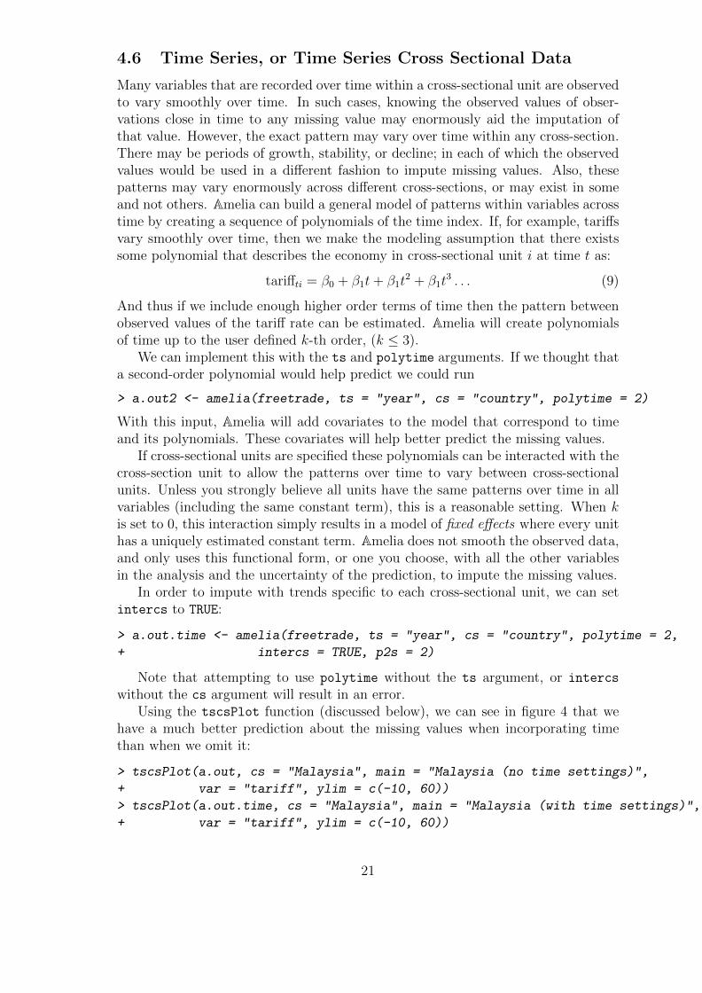
4.6 Time Series, or Time Series Cross Sectional Data
Many variables that are recorded over time within a cross-sectional unit are observedto vary smoothly over time. In such cases, knowing the observed values of obser-vations close in time to any missing value may enormously aid the imputation ofthat value. However, the exact pattern may vary over time within any cross-section.There may be periods of growth, stability, or decline; in each of which the observedvalues would be used in a different fashion to impute missing values. Also, thesepatterns may vary enormously across different cross-sections, or may exist in someand not others. Amelia can build a general model of patterns within variables acrosstime by creating a sequence of polynomials of the time index. If, for example, tariffsvary smoothly over time, then we make the modeling assumption that there existssome polynomial that describes the economy in cross-sectional unit i at time t as:
tariffti = β0 + β1t+ β1t2 + β1t
3 . . . (9)
And thus if we include enough higher order terms of time then the pattern betweenobserved values of the tariff rate can be estimated. Amelia will create polynomialsof time up to the user defined k-th order, (k ≤ 3).
We can implement this with the ts and polytime arguments. If we thought thata second-order polynomial would help predict we could run
> a.out2 <- amelia(freetrade, ts = "year", cs = "country", polytime = 2)
With this input, Amelia will add covariates to the model that correspond to timeand its polynomials. These covariates will help better predict the missing values.
If cross-sectional units are specified these polynomials can be interacted with thecross-section unit to allow the patterns over time to vary between cross-sectionalunits. Unless you strongly believe all units have the same patterns over time in allvariables (including the same constant term), this is a reasonable setting. When kis set to 0, this interaction simply results in a model of fixed effects where every unithas a uniquely estimated constant term. Amelia does not smooth the observed data,and only uses this functional form, or one you choose, with all the other variablesin the analysis and the uncertainty of the prediction, to impute the missing values.
In order to impute with trends specific to each cross-sectional unit, we can setintercs to TRUE:
> a.out.time <- amelia(freetrade, ts = "year", cs = "country", polytime = 2,
+ intercs = TRUE, p2s = 2)
Note that attempting to use polytime without the ts argument, or intercs
without the cs argument will result in an error.Using the tscsPlot function (discussed below), we can see in figure 4 that we
have a much better prediction about the missing values when incorporating timethan when we omit it:
> tscsPlot(a.out, cs = "Malaysia", main = "Malaysia (no time settings)",
+ var = "tariff", ylim = c(-10, 60))
> tscsPlot(a.out.time, cs = "Malaysia", main = "Malaysia (with time settings)",
+ var = "tariff", ylim = c(-10, 60))
21

●
● ●
●●
●● ●
●
●
●
●●
●
●
● ●●
●
1985 1990 1995
−10
010
2030
4050
60
Malaysia (no time settings)
time
tarif
f
● ●
● ●
● ●● ●
●●
●
●●
●●
● ●●
●
1985 1990 1995
−10
010
2030
4050
60
Malaysia (with time settings)
time
tarif
f
Figure 4: The increase in predictive power when using polynomials of time. Thepanels shows mean imputations with 95% bands (in red) and observed data point(in black). The left panel shows an imputation without using time and the rightpanel includes polynomials of time.
4.6.1 Lags and Leads
An alternative way of handling time-series information is to include lags and leads ofcertain variables into the imputation model. Lags are variables that take the valueof another variable in the previous time period while leads take the value of anothervariable in the next time period. Many analysis models use lagged variables to dealwith issues of endogeneity, thus using leads may seems strange. It is important toremember, however, that imputation models are predictive, not causal. Thus, sinceboth past and future values of a variable are likely correlated with the present value,both lags and leads should improve the model.
If we wanted to include lags and leads of tariffs, for instance, we would simplypass this to the lags and leads arguments:
> a.out2 <- amelia(freetrade, ts = "year", cs = "country", lags = "tariff",
+ leads = "tariff")
4.7 Including Prior Information
Amelia has a number of methods of setting priors within the imputation model.Two of these are commonly used and discussed below, ridge priors and observationalpriors.
4.7.1 Ridge Priors for High Missingness, Small n’s, or Large Correla-tions
When the data to be analyzed contain a high degree of missingness or very strongcorrelations among the variables, or when the number of observations is only slightly
22

greater than the number of parameters p(p + 3)/2 (where p is the number of vari-ables), results from your analysis model will be more dependent on the choice ofimputation model. This suggests more testing in these cases of alternative specifica-tions under Amelia. This can happen when using the polynomials of time interactedwith the cross section are included in the imputation model. In our running example,we used a polynomial of degree 2 and there are 9 countries. This adds 3×9−1 = 17more variables to the imputation model (One of the constant “fixed effects” will bedropped so the model will be identified). When these are added, the EM algorithmcan become unstable, as indicated by the vastly differing chain lengths for eachimputation:
> a.out.time
Amelia output with 5 imputed datasets.
Return code: 1
Message: Normal EM convergence.
Chain Lengths:
--------------
Imputation 1: 166
Imputation 2: 212
Imputation 3: 203
Imputation 4: 324
Imputation 5: 128
In these circumstances, we recommend adding a ridge prior which will help withnumerical stability by shrinking the covariances among the variables toward zerowithout changing the means or variances. This can be done by including the empri
argument. Including this prior as a positive number is roughly equivalent to addingempri artificial observations to the data set with the same means and variancesas the existing data but with zero covariances. Thus, increasing the empri settingresults in more shrinkage of the covariances, thus putting more a priori structureon the estimation problem: like many Bayesian methods, it reduces variance inreturn for an increase in bias that one hopes does not overwhelm the advantagesin efficiency. In general, we suggest keeping the value on this prior relatively smalland increase it only when necessary. A recommendation of 0.5 to 1 percent of thenumber of observations, n, is a reasonable starting value, and often useful in largedatasets to add some numerical stability. For example, in a dataset of two thousandobservations, this would translate to a prior value of 10 or 20 respectively. A prior ofup to 5 percent is moderate in most applications and 10 percent is reasonable upperbound.
For our data, it is easy to code up a 1 percent ridge prior:
> a.out.time2 <- amelia(freetrade, ts = "year", cs = "country", polytime = 2,
+ intercs = TRUE, p2s = 0, empri = .01*nrow(freetrade))
> a.out.time2
23

● ●
● ●● ●
● ●
●●
●
●●
●●
● ●●
●
1985 1990 1995
−10
010
2030
4050
60
Malaysia (no ridge prior)
time
tarif
f
●
●●
●●
●● ●
●●
●
●●
●
●
● ●●
●
1985 1990 1995
−10
010
2030
4050
60
Malaysia (with ridge prior)
time
tarif
f
Figure 5: The difference in imputations when using no ridge prior (left) and whenusing a ridge prior set to 1% of the data (right).
Amelia output with 5 imputed datasets.
Return code: 1
Message: Normal EM convergence.
Chain Lengths:
--------------
Imputation 1: 13
Imputation 2: 18
Imputation 3: 22
Imputation 4: 28
Imputation 5: 50
This new imputation model is much more stable and, as shown by using tscsPlot,produces about the same imputations as the original model (see figure 5):
> tscsPlot(a.out.time, cs = "Malaysia", main = "Malaysia (no ridge prior)",
+ var = "tariff", ylim = c(-10, 60))
> tscsPlot(a.out.time2, cs = "Malaysia", main = "Malaysia (with ridge prior)",
+ var = "tariff", ylim = c(-10, 60))
4.7.2 Observation-level priors
Researchers often have additional prior information about missing data values basedon previous research, academic consensus, or personal experience. Amelia can in-corporate this information to produce vastly improved imputations. The Ameliaalgorithm allows users to include informative Bayesian priors about individual miss-ing data cells instead of the more general model parameters, many of which havelittle direct meaning.
24
The incorporation of priors follows basic Bayesian analysis where the imputationturns out to be a weighted average of the model-based imputation and the priormean, where the weights are functions of the relative strength of the data and prior:when the model predicts very well, the imputation will down-weight the prior, andvice versa (Honaker and King, 2010).
The priors about individual observations should describe the analyst’s beliefabout the distribution of the missing data cell. This can either take the form ofa mean and a standard deviation or a confidence interval. For instance, we mightknow that 1986 tariff rates in Thailand around 40%, but we have some uncertaintyas to the exact value. Our prior belief about the distribution of the missing data cell,then, centers on 40 with a standard deviation that reflects the amount of uncertaintywe have about our prior belief.
To input priors you must build a priors matrix with either four or five columns.Each row of the matrix represents a prior on either one observation or one variable.In any row, the entry in the first column is the row of the observation and the entryis the second column is the column of the observation. In the four column priorsmatrix the third and fourth columns are the mean and standard deviation of theprior distribution of the missing value.
For instance, suppose that we had some expert prior information about tariffrates in Thailand. We know from the data that Thailand is missing tariff rates inmany years,
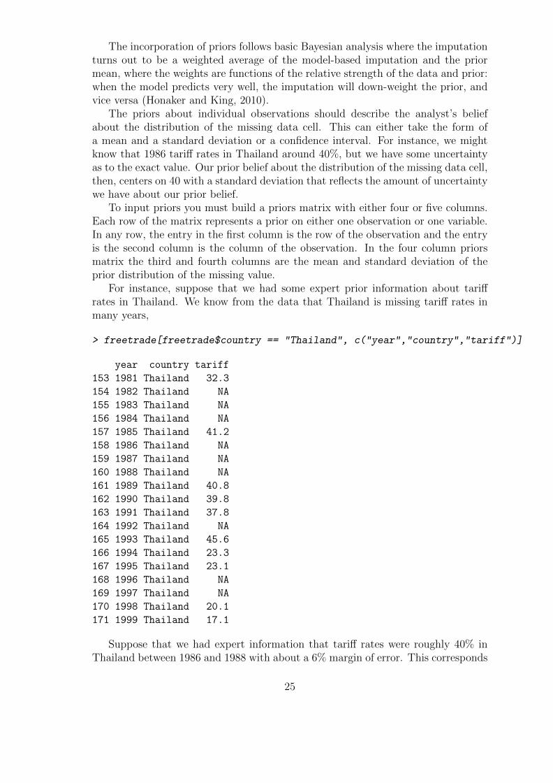
> freetrade[freetrade$country == "Thailand", c("year","country","tariff")]
year country tariff
153 1981 Thailand 32.3
154 1982 Thailand NA
155 1983 Thailand NA
156 1984 Thailand NA
157 1985 Thailand 41.2
158 1986 Thailand NA
159 1987 Thailand NA
160 1988 Thailand NA
161 1989 Thailand 40.8
162 1990 Thailand 39.8
163 1991 Thailand 37.8
164 1992 Thailand NA
165 1993 Thailand 45.6
166 1994 Thailand 23.3
167 1995 Thailand 23.1
168 1996 Thailand NA
169 1997 Thailand NA
170 1998 Thailand 20.1
171 1999 Thailand 17.1
Suppose that we had expert information that tariff rates were roughly 40% inThailand between 1986 and 1988 with about a 6% margin of error. This corresponds
25
to a standard deviation of about 3. In order to include this information, we mustform the priors matrix:
> pr <- matrix(c(158,159,160,3,3,3,40,40,40,3,3,3), nrow=3, ncol=4)
> pr
[,1] [,2] [,3] [,4]
[1,] 158 3 40 3
[2,] 159 3 40 3
[3,] 160 3 40 3
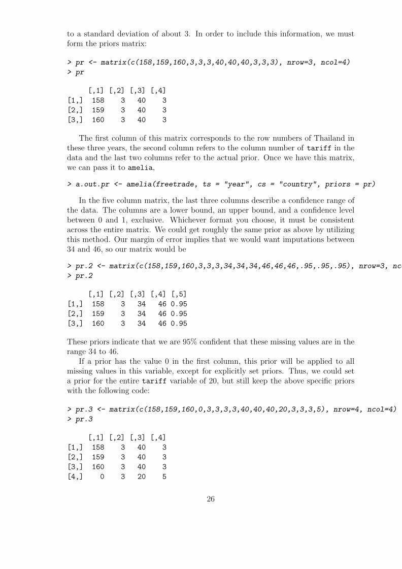
The first column of this matrix corresponds to the row numbers of Thailand inthese three years, the second column refers to the column number of tariff in thedata and the last two columns refer to the actual prior. Once we have this matrix,we can pass it to amelia,
> a.out.pr <- amelia(freetrade, ts = "year", cs = "country", priors = pr)
In the five column matrix, the last three columns describe a confidence range ofthe data. The columns are a lower bound, an upper bound, and a confidence levelbetween 0 and 1, exclusive. Whichever format you choose, it must be consistentacross the entire matrix. We could get roughly the same prior as above by utilizingthis method. Our margin of error implies that we would want imputations between34 and 46, so our matrix would be
> pr.2 <- matrix(c(158,159,160,3,3,3,34,34,34,46,46,46,.95,.95,.95), nrow=3, ncol=5)
> pr.2
[,1] [,2] [,3] [,4] [,5]
[1,] 158 3 34 46 0.95
[2,] 159 3 34 46 0.95
[3,] 160 3 34 46 0.95
These priors indicate that we are 95% confident that these missing values are in therange 34 to 46.
If a prior has the value 0 in the first column, this prior will be applied to allmissing values in this variable, except for explicitly set priors. Thus, we could seta prior for the entire tariff variable of 20, but still keep the above specific priorswith the following code:
> pr.3 <- matrix(c(158,159,160,0,3,3,3,3,40,40,40,20,3,3,3,5), nrow=4, ncol=4)
> pr.3
[,1] [,2] [,3] [,4]
[1,] 158 3 40 3
[2,] 159 3 40 3
[3,] 160 3 40 3
[4,] 0 3 20 5
26
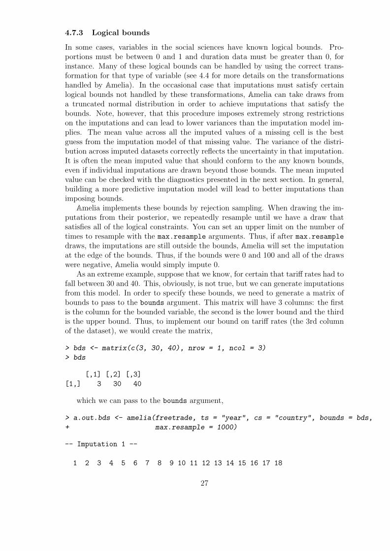
4.7.3 Logical bounds
In some cases, variables in the social sciences have known logical bounds. Pro-portions must be between 0 and 1 and duration data must be greater than 0, forinstance. Many of these logical bounds can be handled by using the correct trans-formation for that type of variable (see 4.4 for more details on the transformationshandled by Amelia). In the occasional case that imputations must satisfy certainlogical bounds not handled by these transformations, Amelia can take draws froma truncated normal distribution in order to achieve imputations that satisfy thebounds. Note, however, that this procedure imposes extremely strong restrictionson the imputations and can lead to lower variances than the imputation model im-plies. The mean value across all the imputed values of a missing cell is the bestguess from the imputation model of that missing value. The variance of the distri-bution across imputed datasets correctly reflects the uncertainty in that imputation.It is often the mean imputed value that should conform to the any known bounds,even if individual imputations are drawn beyond those bounds. The mean imputedvalue can be checked with the diagnostics presented in the next section. In general,building a more predictive imputation model will lead to better imputations thanimposing bounds.
Amelia implements these bounds by rejection sampling. When drawing the im-putations from their posterior, we repeatedly resample until we have a draw thatsatisfies all of the logical constraints. You can set an upper limit on the number oftimes to resample with the max.resample arguments. Thus, if after max.resample
draws, the imputations are still outside the bounds, Amelia will set the imputationat the edge of the bounds. Thus, if the bounds were 0 and 100 and all of the drawswere negative, Amelia would simply impute 0.
As an extreme example, suppose that we know, for certain that tariff rates had tofall between 30 and 40. This, obviously, is not true, but we can generate imputationsfrom this model. In order to specify these bounds, we need to generate a matrix ofbounds to pass to the bounds argument. This matrix will have 3 columns: the firstis the column for the bounded variable, the second is the lower bound and the thirdis the upper bound. Thus, to implement our bound on tariff rates (the 3rd columnof the dataset), we would create the matrix,
> bds <- matrix(c(3, 30, 40), nrow = 1, ncol = 3)
> bds
[,1] [,2] [,3]
[1,] 3 30 40
which we can pass to the bounds argument,
> a.out.bds <- amelia(freetrade, ts = "year", cs = "country", bounds = bds,
+ max.resample = 1000)
-- Imputation 1 --
1 2 3 4 5 6 7 8 9 10 11 12 13 14 15 16 17 18
27
-- Imputation 2 --
1 2 3 4 5 6 7 8 9 10 11 12 13 14 15 16
-- Imputation 3 --
1 2 3 4 5 6 7 8 9 10 11 12 13 14 15
-- Imputation 4 --
1 2 3 4 5 6 7 8 9 10 11 12 13 14 15 16
-- Imputation 5 --
1 2 3 4 5 6 7 8 9 10 11 12 13 14
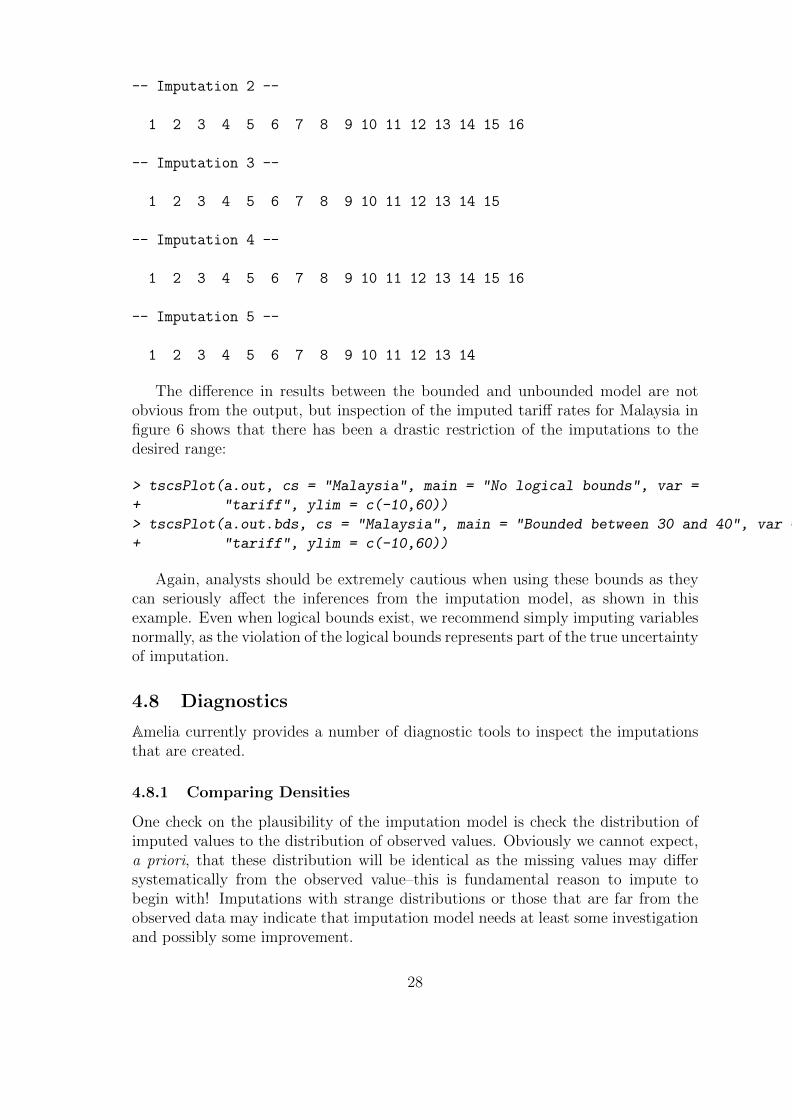
The difference in results between the bounded and unbounded model are notobvious from the output, but inspection of the imputed tariff rates for Malaysia infigure 6 shows that there has been a drastic restriction of the imputations to thedesired range:
> tscsPlot(a.out, cs = "Malaysia", main = "No logical bounds", var =
+ "tariff", ylim = c(-10,60))
> tscsPlot(a.out.bds, cs = "Malaysia", main = "Bounded between 30 and 40", var =
+ "tariff", ylim = c(-10,60))
Again, analysts should be extremely cautious when using these bounds as theycan seriously affect the inferences from the imputation model, as shown in thisexample. Even when logical bounds exist, we recommend simply imputing variablesnormally, as the violation of the logical bounds represents part of the true uncertaintyof imputation.
4.8 Diagnostics
Amelia currently provides a number of diagnostic tools to inspect the imputationsthat are created.
4.8.1 Comparing Densities
One check on the plausibility of the imputation model is check the distribution ofimputed values to the distribution of observed values. Obviously we cannot expect,a priori, that these distribution will be identical as the missing values may differsystematically from the observed value–this is fundamental reason to impute tobegin with! Imputations with strange distributions or those that are far from theobserved data may indicate that imputation model needs at least some investigationand possibly some improvement.
28

●
●
●
●●
●● ●
●
●
●
●●
●
●
● ●●
●
1985 1990 1995
−10
010
2030
4050
60
No logical bounds
time
tarif
f
●
● ● ● ●
●● ●
●
●
●
●●
●
●
● ●●
●
1985 1990 1995
−10
010
2030
4050
60
Bounded between 30 and 40
time
tarif
f
Figure 6: On the left are the original imputations without logical bounds and on theright are the imputation after imposing the bounds.
The plot method works on output from amelia and, by default, shows for eachvariable a plot of the relative frequencies of the observed data with an overlay of therelative frequency of the imputed values.
> plot(a.out, which.vars = 3:6)
where the argument which.vars indicates which of the variables to plot (in thiscase, we are taking the 3rd through the 6th variables).
The imputed curve (in red) plots the density of the mean imputation over the mdatasets. That is, for each cell that is missing in the variable, the diagnostic will findthe mean of that cell across each of the m datasets and use that value for the densityplot. The black distributions are the those of the observed data. When variablesare completely observed, their densities are plotted in blue. These graphs will allowyou to inspect how the density of imputations compares to the density of observeddata. Some discussion of these graphs can be found in Abayomi, Gelman and Levy(2008). Minimally, these graphs can be used to check that the mean imputation fallswithin known bounds, when such bounds exist in certain variables or settings.
We can also use the function compare.density directly to make these plots foran individual variable:
> compare.density(a.out, var = "signed")
4.8.2 Overimpute
Overimputing is a technique we have developed to judge the fit of the imputationmodel. Because of the nature of the missing data mechanism, it is impossible totell whether the mean prediction of the imputation model is close to the unobservedvalue that is trying to be recovered. By definition this missing data does not exist to
29

−20 0 20 40 60 80 100
0.00
00.
010
0.02
00.
030
Observed and Imputed values of tariff
tariff −− Fraction Missing: 0.339
Rel
ativ
e D
ensi
ty
−10 −5 0 5 10 15
0.0
0.2
0.4
0.6
0.8
Observed and Imputed values of polity
polity −− Fraction Missing: 0.012
Rel
ativ
e D
ensi
ty
0e+00 4e+08 8e+08
0e+
004e
−09
8e−
09
Observed values of pop
N = 171 Bandwidth = 2.431e+07
Den
sity
0 5000 10000
0e+
002e
−04
4e−
04Observed values of gdp.pc
N = 171 Bandwidth = 490.6
Den
sity
Figure 7: The output of the plot method as applied to output from amelia. Inthe upper panels, the distribution of mean imputations (in red) is overlayed on thedistribution of observed values (in black) for each variable. In the lower panels, thereare no missing values and the distribution of observed values is simply plotted (inblue). Note that now imputed tariff rates are very similar to observed tariff rates,but the imputation of the Polity score are quite different. This is plausible if differenttypes of regimes tend to be missing at different rates.
30

create this comparison, and if it existed we would no longer need the imputations orcare about their accuracy. However, a natural question the applied researcher willoften ask is how accurate are these imputed values?
Overimputing involves sequentially treating each of the observed values as ifthey had actually been missing. For each observed value in turn we then generateseveral hundred imputed values of that observed value, as if it had been missing.While m = 5 imputations are sufficient for most analysis models, this large numberof imputations allows us to construct a confidence interval of what the imputedvalue would have been, had any of the observed data been missing. We can thengraphically inspect whether our observed data tends to fall within the region whereit would have been imputed had it been missing.
For example, we can run the overimputation diagnostic on our data by running
> overimpute(a.out, var = "tariff")
Our overimputation diagnostic, shown in Figure 8, runs this procedure throughall of the observed values for a user selected variable. We can graph the estimates ofeach observation against the true values of the observation. On this graph, a y = xline indicates the line of perfect agreement; that is, if the imputation model was aperfect predictor of the true value, all the imputations would fall on this line. Foreach observation, Amelia also plots 90% confidence intervals that allows the user tovisually inspect the behavior of the imputation model. By checking how many ofthe confidence intervals cover the y = x line, we can tell how often the imputationmodel can confidently predict the true value of the observation.
Occasionally, the overimputation can display unintuitive results. For example,different observations may have different numbers of observed covariates. If covari-ates that are useful to the prediction are themselves missing, then the confidenceinterval for this observation will be much larger. In the extreme, there may be ob-servations where the observed value we are trying to overimpute is the only observedvalue in that observation, and thus there is nothing left to impute that observationwith when we pretend that it is missing, other than the mean and variance of thatvariable. In these cases, we should correctly expect the confidence interval to bevery large.
An example of this graph is shown in figure 9. In this simulated bivariate dataset,one variable is overimputed and the results displayed. The second variable is eitherobserved, in which case the confidence intervals are very small and the imputa-tions (yellow) are very accurate, or the second variable is missing in which case thisvariable is being imputed simply from the mean and variance parameters, and theimputations (red) have a very large and encompassing spread. The circles representthe mean of all the imputations for that value. As the amount of missing informationin a particular pattern of missingness increases, we expect the width of the confi-dence interval to increase. The color of the confidence interval reflects the percentof covariates observed in that pattern of missingness, as reflected in the legend atthe bottom.
31

20 40 60 80 100
−40
−20
020
4060
8010
0Observed versus Imputed Values of tariff
Observed Values
Impu
ted
Val
ues
0−.2 .2−.4 .4−.6 .6−.8 .8−1
Figure 8: An example of the overimputation diagnostic graph. Here ninety percentconfidence intervals are constructed that detail where an observed value would havebeen imputed had it been missing from the dataset, given the imputation model.The dots represent the mean imputation. Around ninety percent of these confidenceintervals contain the y = x line, which means that the true observed value fallswithin this range. The color of the line (as coded in the legend) represents thefraction of missing observations in the pattern of missingness for that observation.
32

0.0 0.5 1.0
0.0
0.5
1.0
Observed versus Imputed Values
Observed Values
Impu
ted
Val
ues
0−.2 .2−.4 .4−.6 .6−.8 .8−1
Figure 9: Another example of the overimpute diagnostic graph. Note that the redlines are those observations that have fewer covariates observed and have a highervariance across the imputed values.
33
4.8.3 Overdispersed Starting Values
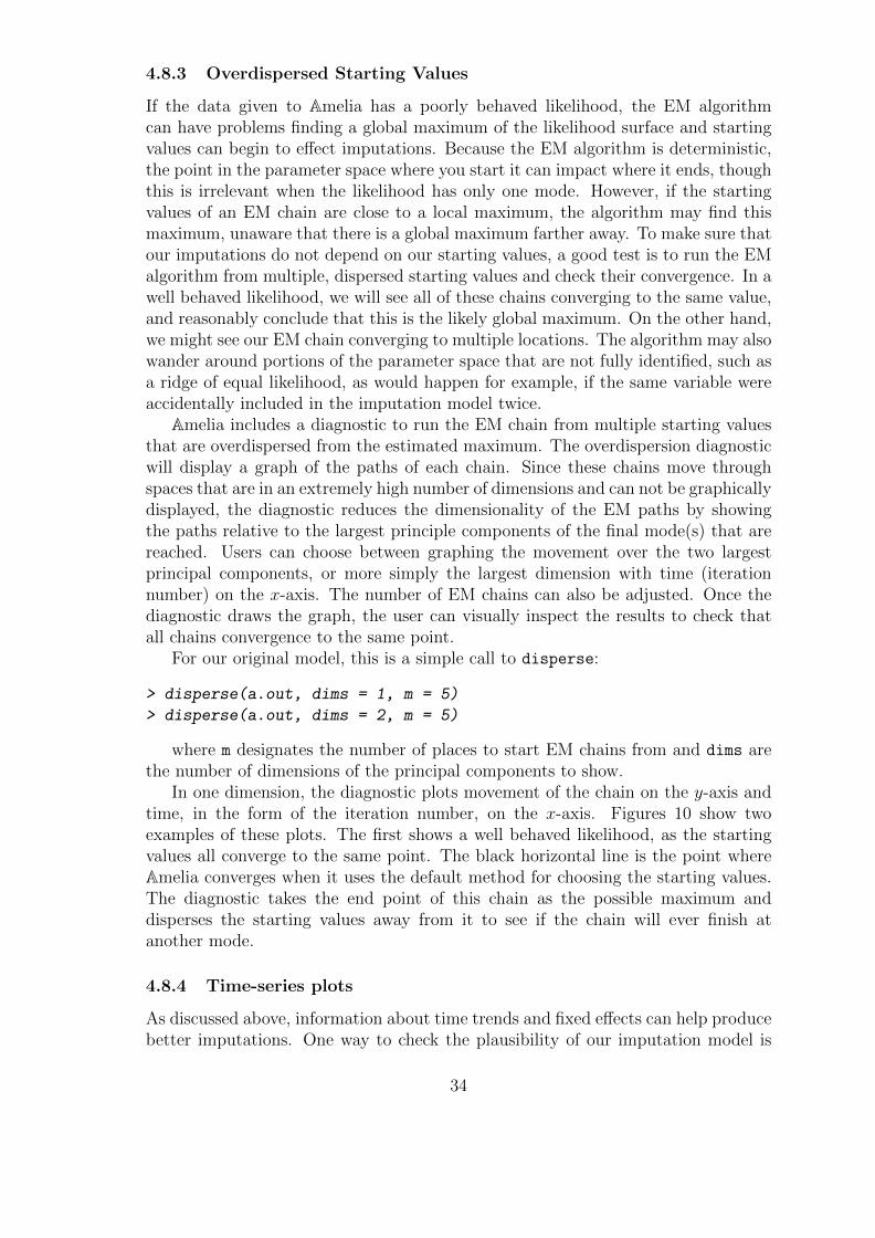
If the data given to Amelia has a poorly behaved likelihood, the EM algorithmcan have problems finding a global maximum of the likelihood surface and startingvalues can begin to effect imputations. Because the EM algorithm is deterministic,the point in the parameter space where you start it can impact where it ends, thoughthis is irrelevant when the likelihood has only one mode. However, if the startingvalues of an EM chain are close to a local maximum, the algorithm may find thismaximum, unaware that there is a global maximum farther away. To make sure thatour imputations do not depend on our starting values, a good test is to run the EMalgorithm from multiple, dispersed starting values and check their convergence. In awell behaved likelihood, we will see all of these chains converging to the same value,and reasonably conclude that this is the likely global maximum. On the other hand,we might see our EM chain converging to multiple locations. The algorithm may alsowander around portions of the parameter space that are not fully identified, such asa ridge of equal likelihood, as would happen for example, if the same variable wereaccidentally included in the imputation model twice.
Amelia includes a diagnostic to run the EM chain from multiple starting valuesthat are overdispersed from the estimated maximum. The overdispersion diagnosticwill display a graph of the paths of each chain. Since these chains move throughspaces that are in an extremely high number of dimensions and can not be graphicallydisplayed, the diagnostic reduces the dimensionality of the EM paths by showingthe paths relative to the largest principle components of the final mode(s) that arereached. Users can choose between graphing the movement over the two largestprincipal components, or more simply the largest dimension with time (iterationnumber) on the x-axis. The number of EM chains can also be adjusted. Once thediagnostic draws the graph, the user can visually inspect the results to check thatall chains convergence to the same point.
For our original model, this is a simple call to disperse:
> disperse(a.out, dims = 1, m = 5)
> disperse(a.out, dims = 2, m = 5)
where m designates the number of places to start EM chains from and dims arethe number of dimensions of the principal components to show.
In one dimension, the diagnostic plots movement of the chain on the y-axis andtime, in the form of the iteration number, on the x-axis. Figures 10 show twoexamples of these plots. The first shows a well behaved likelihood, as the startingvalues all converge to the same point. The black horizontal line is the point whereAmelia converges when it uses the default method for choosing the starting values.The diagnostic takes the end point of this chain as the possible maximum anddisperses the starting values away from it to see if the chain will ever finish atanother mode.
4.8.4 Time-series plots
As discussed above, information about time trends and fixed effects can help producebetter imputations. One way to check the plausibility of our imputation model is
34

0 5 10 15
−0.
50.
00.
51.
0
Overdispersed Start Values
Number of Iterations
Larg
est P
rinci
ple
Com
pone
nt
Convergence of original starting values
1.0 1.5 2.0 2.5 3.0
0.0
0.2
0.4
0.6
0.8
1.0
1.2
Overdispersed Starting Values
First Principle Component
Sec
ond
Prin
cipl
e C
ompo
nent
Figure 10: A plot from the overdispersion diagnostic where all EM chains are con-verging to the same mode, regardless of starting value. On the left, the y-axisrepresents movement in the (very high dimensional) parameter space, and the x-axis represents the iteration number of the chain. On the right, we visualize theparameter space in two dimensions using the first two principal components of theend points of the EM chains. The iteration number is no longer represented on they-axis, although the distance between iterations is marked by the distance betweenarrowheads on each chain.
to see how it predicts missing values in a time series. If the imputations for theMalaysian tariff rate were drastically higher in 1990 than the observed years of 1989or 1991, we might worry that there is a problem in our imputation model. Checkingthese time series is easy to do with the tscsPlot command. Simply choose thevariable (with the var argument) and the cross-section (with the cs argument) toplot the observed time-series along with distributions of the imputed values for eachmissing time period. For instance, we can run
> tscsPlot(a.out.time, cs = "Malaysia", main = "Malaysia (with time settings)",
+ var = "tariff", ylim = c(-10, 60))
to get the plot in figure 11. Here, the black point are observed tariff rates forMalaysia from 1980 to 2000. The red points are the mean imputation for each ofthe missing values, along with their 95% confidence bands. We draw these bandsby imputing each of missing values 100 times to get the imputation distribution forthat observation.
to get the plot in figure 11. Here, the black point are observed tariff rates forMalaysia from 1980 to 2000. The red points are the mean imputation for each ofthe missing values, along with their 95% confidence bands. We draw these bandsby imputing each of missing values 100 times to get the imputation distribution forthat observation.
35

● ●
● ●●
●
● ●
●●
●
●●
●●
● ●
●●
1985 1990 1995
−10
010
2030
4050
60
Malaysia (with time settings)
time
tarif
f
Figure 11: Tariff rates in Malaysia, 1980-2000. An example of the tscsPlot function,the black points are observed values of the time series and the red points are themean of the imputation distributions. The red lines represent the 95% confidencebands of the imputation distribution.
36

In figure 11, we can see that the imputed 1990 tariff rate is quite in line withthe values around it. Notice also that values toward the beginning and end of thetime series have higher imputation variance. This occurs because the fit of thepolynomials of time in the imputation model have higher variance at the beginningand end of the time series. This is intuitive because these points have fewer neighborsfrom which to draw predictive power.
A word of caution is in order. As with comparing the histograms of imputed andobserved values, there could be reasons that the missing values are systematicallydifferent than the observed time series. For instance, if there had been a majorfinancial crisis in Malaysia in 1990 which caused the government to close off trade,then we would expect that the missing tariff rates should be quite different thanthe observed time series. If we have this information in our imputation model, wemight expect to see out-of-line imputations in these time-series plots. If, on theother hand, we did not have this information, we might see “good” time-series plotsthat fail to point out this violation of the MAR assumption. Our imputation modelwould produce poor estimates of the missing values since it would be unaware thatboth the missingness and the true unobserved tariff rate depend on another variable.Hence, the tscsPlot is useful for finding obvious problems in imputation model andcomparing the efficiency of various imputation models, but it cannot speak to theuntestable assumption of MAR.
4.8.5 Missingness maps
One useful tool for exploring the missingness in a dataset is a missingness map. Thisis a map that visualizes the dataset a grid and colors the grid by missingness status.The column of the grid are the variables and the rows are the observations, as inany spreadsheet program. This tool allows for a quick summary of the patterns ofmissingness in the data.
If we simply call the missmap function on our output from amelia,
> missmap(a.out)
we get the plot in figure 12. The missmap function arrange the columns so that thevariables are in decreasing order of missingness from left to right. If the cs argumentwas set in the amelia function, the labels for the rows will indicate where each ofthe cross-sections begin.
In figure 12, it is clear that the tariff rate is the variable most missing in thedata and it tends to be missing in blocks of a few observations. Gross internationalreserves (intresmi) and financial openness (fivop), on the other hand, are missingmostly at the end of each cross-section. This suggests missingness by merging,when variables with different temporal coverages are merged to make one dataset.Sometimes this kind of missingness is an artifact of the date at which the data wasmerged and researchers can resolve it by finding updated versions of the relevantvariables.
The missingness map is an important tool for understanding the patterns of miss-ingness in the data and can often indicate potential ways to improve the imputationmodel or data collection process.
37

Missingness Mapta
riff
fiveo
p
intr
esm
i
sign
ed
polit
y
ushe
g
gdp.
pc
pop
coun
try
year
Thailand
SriLanka
Philippines
Pakistan
Nepal
Malaysia
Korea
Indonesia
India
Missing (5%)Observed (95%)
Figure 12: Missingness map of the freetrade data. Missing values are in tan andobserved values are in red.
38

4.9 Post-imputation Transformations
In many cases, it is useful to create transformations of the imputed varibles for usein further analysis. For instance, one may want to create an interaction betweentwo variables or perform a log-transformation on the imputed data. To do this,Amelia includes a transform function for amelia output that adds or overwritesvariables in each of the imputed datasets. For instance, if we wanted to create alog-transformation of the gdp.pc variable, we could use the following command:
> a.out <- transform(a.out, lgdp = log(gdp.pc))
> head(a.out$imputations[[1]][,c("country", "year","gdp.pc", "lgdp")])
country year gdp.pc lgdp
1 SriLanka 1981 461.0 6.133
2 SriLanka 1982 473.8 6.161
3 SriLanka 1983 489.2 6.193
4 SriLanka 1984 508.2 6.231
5 SriLanka 1985 525.6 6.264
6 SriLanka 1986 538.9 6.290
To create an interaction between two variables, we could simply use:
> a.out <- transform(a.out, pol_gdp = polity * gdp.pc)
Each transformation is recorded and the summary command prints out each trans-formation that has been performed:
> summary(a.out)
Amelia output with 5 imputed datasets.
Return code: 1
Message: Normal EM convergence.
Chain Lengths:
--------------
Imputation 1: 14
Imputation 2: 15
Imputation 3: 9
Imputation 4: 14
Imputation 5: 10
Rows after Listwise Deletion: 96
Rows after Imputation: 171
Patterns of missingness in the data: 8
Fraction Missing for original variables:
-----------------------------------------
Fraction Missing
39

year 0.00000
country 0.00000
tariff 0.33918
polity 0.01170
pop 0.00000
gdp.pc 0.00000
intresmi 0.07602
signed 0.01754
fiveop 0.10526
usheg 0.00000
lgdp 0.00000
pol_gdp 0.01170
Post-imputation transformed variables:
-----------------------------------------
Transformations
lgdp = log(gdp.pc)
pol_gdp = polity * gdp.pc
Note the updated output is almost exactly the same as the fresh amelia output.You can pass the transformed output back to amelia and it will add imputationsand update these imputations with the transformations you have performed.
4.10 Analysis Models
Imputation is most often a data processing step as opposed to a final model in ofitself. To this end, it is easy to pass output from amelia to other functions. Theeasiest and most integrated way to run an analysis model is to pass the output tothe zelig function from the Zelig package. For example, in Milner and Kubota(2005), the dependent variable was tariff rates. We can replicate table 5.1 from theiranalysis with the original data simply by running
> require(Zelig)
> z5 <- zls$new()
> z5$zelig(tariff ~ polity + pop + gdp.pc + year + country, data = freetrade)
> z5
Model:
Call:
z5$zelig(formula = tariff ~ polity + pop + gdp.pc + year + country,
data = freetrade)
Residuals:
Min 1Q Median 3Q Max
40

-30.764 -3.259 0.087 2.598 18.310
Coefficients:
Estimate Std. Error t value Pr(>|t|)
(Intercept) 1.97e+03 4.02e+02 4.91 3.6e-06
polity -1.37e-01 1.82e-01 -0.75 0.45
pop -2.02e-07 2.54e-08 -7.95 3.2e-12
gdp.pc 6.10e-04 7.44e-04 0.82 0.41
year -8.71e-01 2.08e-01 -4.18 6.4e-05
countryIndonesia -1.82e+02 1.86e+01 -9.82 3.0e-16
countryKorea -2.20e+02 2.08e+01 -10.61 < 2e-16
countryMalaysia -2.25e+02 2.17e+01 -10.34 < 2e-16
countryNepal -2.16e+02 2.25e+01 -9.63 7.7e-16
countryPakistan -1.55e+02 1.98e+01 -7.84 5.6e-12
countryPhilippines -2.04e+02 2.09e+01 -9.77 3.7e-16
countrySriLanka -2.09e+02 2.21e+01 -9.46 1.8e-15
countryThailand -1.96e+02 2.10e+01 -9.36 3.0e-15
Residual standard error: 6.22 on 98 degrees of freedom
(60 observations deleted due to missingness)
Multiple R-squared: 0.925, Adjusted R-squared: 0.915
F-statistic: 100 on 12 and 98 DF, p-value: <2e-16
Statistical Warning: The GIM test suggests this model is misspecified
(based on comparisons between classical and robust SE's; see http://j.mp/GIMtest).
We suggest you run diagnostics to ascertain the cause, respecify the model
and run it again.
Next step: Use 'setx' method
Running the same model with imputed data is almost identical. Simply replacethe original data set with the amelia output:
> z5 <- zls$new()
> z5$zelig(tariff ~ polity + pop + gdp.pc + year + country, data = a.out)
> z5
Model: Combined Imputations
Estimate Std.Error z value Pr(>|z|)
(Intercept) 2.6e+03 6.0e+02 4.3 2e-05
polity 3.3e-01 3.0e-01 1.1 0.278
pop -1.1e-07 4.3e-08 -2.5 0.012
gdp.pc -2.3e-04 1.3e-03 -0.2 0.855
year -1.2e+00 3.1e-01 -3.9 9e-05
countryIndonesia -1.0e+02 3.1e+01 -3.3 9e-04
41
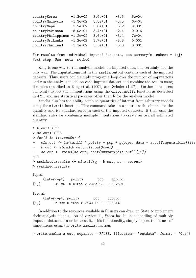
countryKorea -1.3e+02 3.6e+01 -3.5 5e-04
countryMalaysia -1.3e+02 3.8e+01 -3.5 6e-04
countryNepal -1.2e+02 3.8e+01 -3.2 0.001
countryPakistan -8.0e+01 3.4e+01 -2.4 0.016
countryPhilippines -1.2e+02 3.6e+01 -3.4 7e-04
countrySriLanka -1.2e+02 3.7e+01 -3.3 0.001
countryThailand -1.1e+02 3.5e+01 -3.3 0.001
For results from individual imputed datasets, use summary(x, subset = i:j)
Next step: Use 'setx' method
Zelig is one way to run analysis models on imputed data, but certainly not theonly way. The imputations list in the amelia output contains each of the imputeddatasets. Thus, users could simply program a loop over the number of imputationsand run the analysis model on each imputed dataset and combine the results usingthe rules described in King et al. (2001) and Schafer (1997). Furthermore, userscan easily export their imputations using the write.amelia function as describedin 4.2.1 and use statistical packages other than R for the analysis model.
Amelia also has the ability combine quantities of interest from arbitrary modelsusing the mi.meld function. This command takes in a matrix with columns for thequantity and its standard error in each of the imputed datasets. It then uses thestandard rules for combining multiple imputations to create an overall estimatedquantity.
> b.out<-NULL
> se.out<-NULL
> for(i in 1:a.out$m) {
+ ols.out <- lm(tariff ~ polity + pop + gdp.pc, data = a.out$imputations[[i]])
+ b.out <- rbind(b.out, ols.out$coef)
+ se.out <- rbind(se.out, coef(summary(ols.out))[,2])
+ }
> combined.results <- mi.meld(q = b.out, se = se.out)
> combined.results
$q.mi
(Intercept) polity pop gdp.pc
[1,] 31.86 -0.01699 3.345e-08 -0.002591
$se.mi
(Intercept) polity pop gdp.pc
[1,] 2.338 0.2699 6.394e-09 0.0006314
In addition to the resources available in R, users can draw on Stata to implementtheir analysis models. As of version 11, Stata has built-in handling of multiplyimputed datasets. In order to utilize this functionality, simply export the “stacked”imputations using the write.amelia function:
> write.amelia(a.out, separate = FALSE, file.stem = "outdata", format = "dta")
42

Once this stacked dataset is open in Stata, you must tell Stata that it is animputed dataset using the mi import flong command:
mi import flong, m(imp) id(year country) imp(tariff-usheg)
The command takes a few options: m designates the imputation variable (set withimpvar in write.amelia), id sets the identifying varibles, and imp sets the variablesthat were imputed (or included in the imputation). The tariff-usheg indicates thatStata should treat the range of variables between tariff and usheg as imputed.Once we have set the dataset as imputed, we can use the built-in mi commands toanalyze the data:
. mi estimate: reg tariff polity pop gdp_pc
Multiple-imputation estimates Imputations = 5
Linear regression Number of obs = 171
Average RVI = 1.4114
Complete DF = 167
DF adjustment: Small sample DF: min = 10.36
avg = 18.81
max = 37.62
Model F test: Equal FMI F( 2, 10.4) = 15.50
Within VCE type: OLS Prob > F = 0.0008
------------------------------------------------------------------------------
tariff | Coef. Std. Err. t P>|t| [95% Conf. Interval]
-------------+----------------------------------------------------------------
polity | -.2058115 .3911049 -0.53 0.610 -1.072968 .6613452
pop | 3.21e-08 8.72e-09 3.68 0.004 1.27e-08 5.14e-08
gdp_pc | -.0027561 .000644 -4.28 0.000 -.0040602 -.0014519
_cons | 32.70461 2.660091 12.29 0.000 27.08917 38.32005
------------------------------------------------------------------------------
4.11 The amelia class
The output from the amelia function is an instance of the S3 class “amelia.” In-stances of the amelia class contain much more than simply the imputed datasets.The mu object of the class contains the posterior draws of the means of the completedata. The covMatrices contains the posterior draws of the covariance matrices ofthe complete data. Note that these correspond to the variables as they are sentto the EM algorithm. Namely, they refer to the variables after being transformed,centered and scaled.
The iterHist object is a list of m 3-column matrices. Each row of the matricescorresponds to an iteration of the EM algorithm. The first column indicates howmany parameters had yet to converge at that iteration. The second column indicatesif the EM algorithm made a step that decreased the number of converged parameters.The third column indicates whether the covariance matrix at this iteration was
43

singular. Clearly, the last two columns are meant to indicate when the EM algorithmenters a problematic part of the parameter space.
44

5 AmeliaView Menu Guide
Below is a guide to the AmeliaView menus with references back to the users’s guide.The same principles from the user’s guide apply to AmeliaView. The only differenceis how you interact with the program. Whether you use the GUI or the commandline versions, the same underlying code is being called, and so you can read thecommand line-oriented discussion above even if you intend to use the GUI.
5.1 Loading AmeliaView
The easiest way to load AmeliaView is to open an R session and type the followingtwo commands:
> library(Amelia)
> AmeliaView()
This will bring up the AmeliaView window on any platform.On the Windows operating system, there is an alternative way to start AmeliaView
from the Desktop. See section 3.2 for a guide on how to install this version. Onceinstalled, there should be a Desktop icon for AmeliaView. Simply double-click thisicon and the AmeliaView window should appear. If, for some reason, this approachdoes not work, simply open an R session and use the approach above.
5.2 Loading a data set into AmeliaView
AmeliaView load with a welcome screen (Figure 13) that has buttons which can loada data in many of the common formats. Each of these will bring up a window forchoosing your dataset. Note that these buttons are only a subset of the possibleways to load data in AmeliaView. Under the File menu (shown in Figure 14), youwill find more options, including the datasets included in the package (africa andfreetrade). You will also find import commands for Comma-Separated Values(.CSV), Tab-Delimited Text (.TXT), Stata v.5-10 (.DTA), SPSS (.DAT), and SASTransport (.XPORT). Note that when using a CSV file, Amelia assumes that yourfile has a header (that is, a row at the top of the data indicating the variable names).
You can also load data from an RData file. If the RData file contains more thanone data.frame, a pop-up window will ask to you find the dataset you would like toload. In the file menu, you can also change the underlying working directory. Thisis where AmeliaView will look for data by default and where it will save imputeddatasets.
5.3 Variable dashboard
Once a dataset is loaded, AmeliaView will show the variable dashboard (Figure 15).In this mode, you will see a table of variables, with the current options for each ofthem shown, along with a few summary statistics. You can reorder this table byany of these columns by clicking on the column headings. This might be helpful to,say, order the variables by mean or amount of missingness.
45

Figure 13: AmeliaView welcome screen.
You can set options for individual variables by the right-click context menu (Fig-ure 16) or through the Variables menu. For instance, clicking “Set as Time-SeriesVariable” will set the currently selected variable in the dashboard as the time-seriesvariable. Certain options are disabled until other options are enabled. For instance,you cannot add a lagged variable to the imputation until you have set the time-seriesvariable. Note that any factor in the data is marked as a ID variable by default,since a factor cannot be included in the imputation without being set as an IDvariable, a nominal variable, or the cross-section variable. If there is a factor thatfails to meet one of these conditions, a red flag will appear next to the variable name.
1. Set as Time-Series Variable - Sets the currently selected variable to thetime-series variable. Disabled when more than one variable is selected. Oncethis is set, you can add lags and leads and add splines of time. The time-seriesvariable will have a clock icon next to it.
2. Set as Cross-Section Variable - Sets the currently selected variable tothe cross-section variable. Disabled when more than one variable is selected.Once this is set, you can interact the splines of time with the cross-section.The cross-section variable will have a person icon next to it.
3. Unset as Time-Series Variable - Removes the time-series status of thevariable. This will remove any lags, leads, or splines of time.
4. Unset as Cross-Section Variable - Removes the cross-section status of
46

Figure 14: AmeliaViewFile and import menu.
the variable. This will remove any intersection of the splines of time and thecross-section.
5. Add Lag/Lead - Adds versions of the selected variables either lagged back(“lag”) or forward(“lead”). See 4.6.1 above.
6. Remove Lag/Lead - Removes any lags or leads on the selected variables.
7. Plot Histogram of Selected - Plots a histogram of the selected variables.This command will attempt to put all of the histograms on one page, but ifmore than nine histograms are requested, they will appear on multiple pages.
8. Add Transformation... - Adds a transformation setting for the selectedvariables. Note that each variable can only have one transformation and thetime-series and cross-section variables cannot be transformed.
9. Remove Transformation - Removes any transformation for the selectedvariables.
10. Add or Edit Bounds - Opens a dialog box to set logical bounds for theselected variable.
5.4 Amelia Options
The Variable menu and the variable dashboard are the place to set variable-leveloptions, but global options are set in the Options menu.
1. Splines of Time with... - This option, if activated, will have Amelia useflexible trends of time with the specified number of knots in the imputation.The higher the number of knots the greater the variation in the trend structure,yet it will take more degrees of freedom to estimate. For more information see4.6 above.
2. Interact with Cross-Section? - Include and interaction of the cross-sectionwith the time trends. This interaction is way of allowing the trend of time tovary across cases as well. Using a 0-level spline of time and interacting withthe cross section is the equivalent of using a fixed effects. For more informationsee 4.6 above.
47

Figure 15: Main variable dashboard in AmeliaView.
3. Add Observational Priors... - Brings a dialog window to set prior beliefsabout ranges for individual missing observations. For more information aboutobservational priors, see 4.7.2.
4. Numerical Options - Brings a dialog window to set the tolerance of the EMalgorithm, the seed of the random number generator, the ridge prior for nu-merical stability, and the maximum number of redraws for the logical bounds.
5. Draw Missingness Map - Draws a missingness map. See 4.8.5 for moredetails on missingness maps.
6. Output File Options - Bring a dialog to set the stub of the prefix of theimputed data files and the number of imputations. If you set the prefix to“mydata”, your output files will be mydata1.csv, mydata2.csv... etc.
7. Output File Type - Sets the format of imputed data. If you would like tonot save any output data sets (if you wanted, for instance, to simply look atdiagnostics), set this option to “(no save).” Currently, you can save the outputdata as: Comma Separated Values (.CSV), Tab Delimited Text (.TXT), Stata(.DTA), R save object (.RData), or to hold it in R memory. This last optionwill only work if you have called AmeliaView from an R session and wantto return to the R command line to work with the output. Its name in Rworkspace will be the file prefix. The stacked version of the Stata output willwork with their built-in mi tools.
48
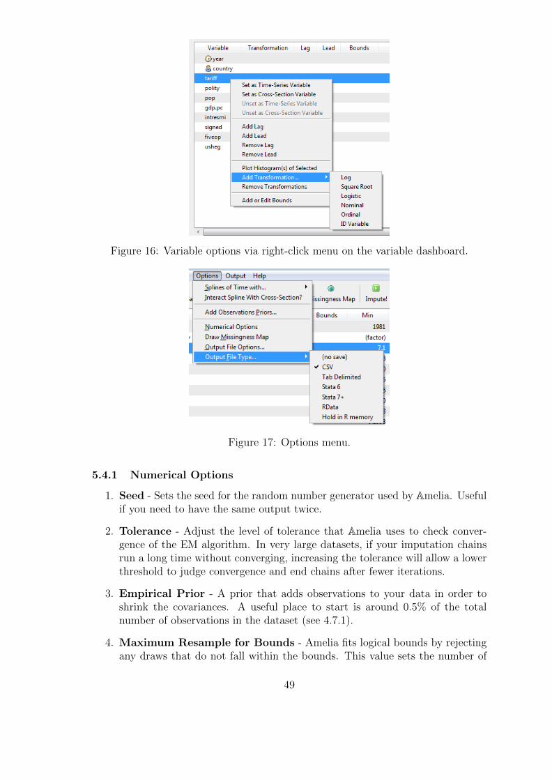
Figure 16: Variable options via right-click menu on the variable dashboard.
Figure 17: Options menu.
5.4.1 Numerical Options
1. Seed - Sets the seed for the random number generator used by Amelia. Usefulif you need to have the same output twice.
2. Tolerance - Adjust the level of tolerance that Amelia uses to check conver-gence of the EM algorithm. In very large datasets, if your imputation chainsrun a long time without converging, increasing the tolerance will allow a lowerthreshold to judge convergence and end chains after fewer iterations.
3. Empirical Prior - A prior that adds observations to your data in order toshrink the covariances. A useful place to start is around 0.5% of the totalnumber of observations in the dataset (see 4.7.1).
4. Maximum Resample for Bounds - Amelia fits logical bounds by rejectingany draws that do not fall within the bounds. This value sets the number of
49

Figure 18: Options menu.
times Amelia should attempt to resample to fit the bounds before setting theimputation to the bound.
5.4.2 Add Distribution Prior
Figure 19: Detail for Add Distributional Prior dialog
1. Current Priors - A table of current priors in distributional form, with thevariable and case name. You can remove priors by selecting them and usingthe right-click context menu.
2. Case - Select the case name or number you wish to set the prior about. Youcan also choose to make the prior for the entire variable, which will set theprior for any missing cell in that variable. The case names are generated fromthe row name of the observation, the value of the cross-section variable of theobservation and the value of the time series variable of the observation.
3. Variable - The variable associated with the prior you would like specify. Thelist provided only shows the missing variables for the currently selected obser-vation.
50

4. Mean - The mean value of the prior. The textbox will not accept letters orout of place punctuation.
5. Standard Deviation - The standard deviation of the prior. The textbox willonly accept positive non-zero values.
5.4.3 Add Range Prior
Figure 20: Detail for Add Range Prior dialog.
1. Case - Select the case name or number you wish to set the prior about. Youcan also choose to make the prior for the entire variable, which will set theprior for any missing cell in that variable. The case names are generated fromthe row name of the observation, the value of the cross-section variable of theobservation and the value of the time series variable of the observation.
2. Variable - The variable associated with the prior you would like specify. Thelist provided only shows the missing variables for the currently selected obser-vation.
3. Minimum - The minimum value of the prior. The textbox will not acceptletters or out of place punctuation.
4. Maximum - The maximum value of the prior. The textbox will not acceptletters or out of place punctuation.
5. Confidence - The confidence level of the prior. This should be between 0 and1, non-inclusive. This value represents how certain your priors are. This valuecannot be 1, even if you are absolutely certain of a give range. This is used toconvert the range into an appropriate distributional prior.
51
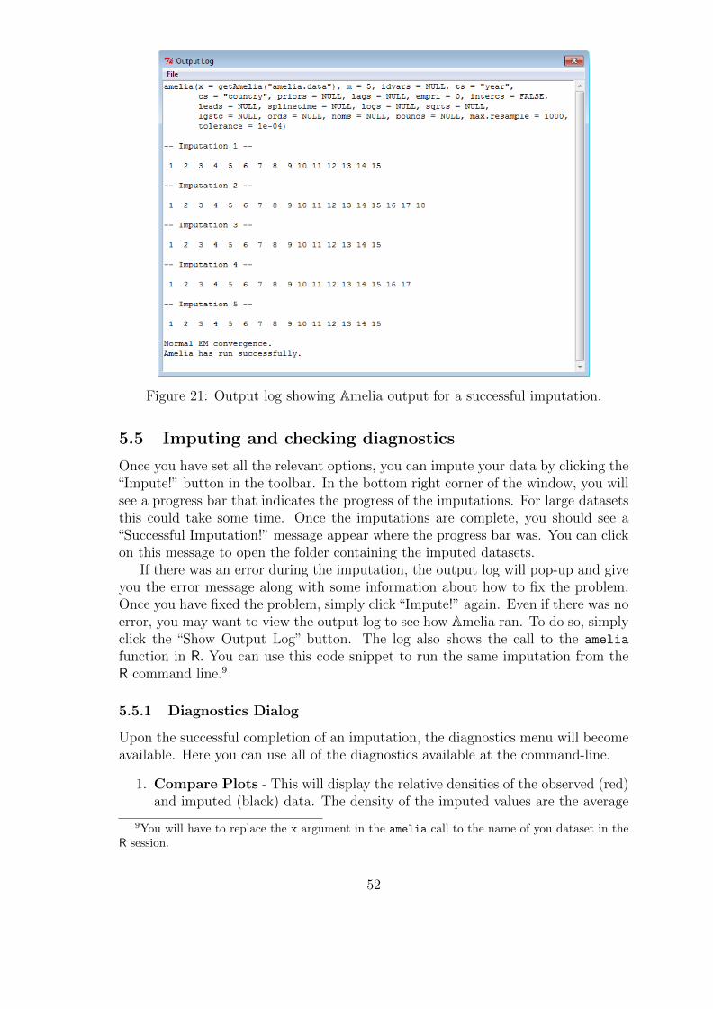
Figure 21: Output log showing Amelia output for a successful imputation.
5.5 Imputing and checking diagnostics
Once you have set all the relevant options, you can impute your data by clicking the“Impute!” button in the toolbar. In the bottom right corner of the window, you willsee a progress bar that indicates the progress of the imputations. For large datasetsthis could take some time. Once the imputations are complete, you should see a“Successful Imputation!” message appear where the progress bar was. You can clickon this message to open the folder containing the imputed datasets.
If there was an error during the imputation, the output log will pop-up and giveyou the error message along with some information about how to fix the problem.Once you have fixed the problem, simply click “Impute!” again. Even if there was noerror, you may want to view the output log to see how Amelia ran. To do so, simplyclick the “Show Output Log” button. The log also shows the call to the amelia
function in R. You can use this code snippet to run the same imputation from theR command line.9
5.5.1 Diagnostics Dialog
Upon the successful completion of an imputation, the diagnostics menu will becomeavailable. Here you can use all of the diagnostics available at the command-line.
1. Compare Plots - This will display the relative densities of the observed (red)and imputed (black) data. The density of the imputed values are the average
9You will have to replace the x argument in the amelia call to the name of you dataset in theR session.
52
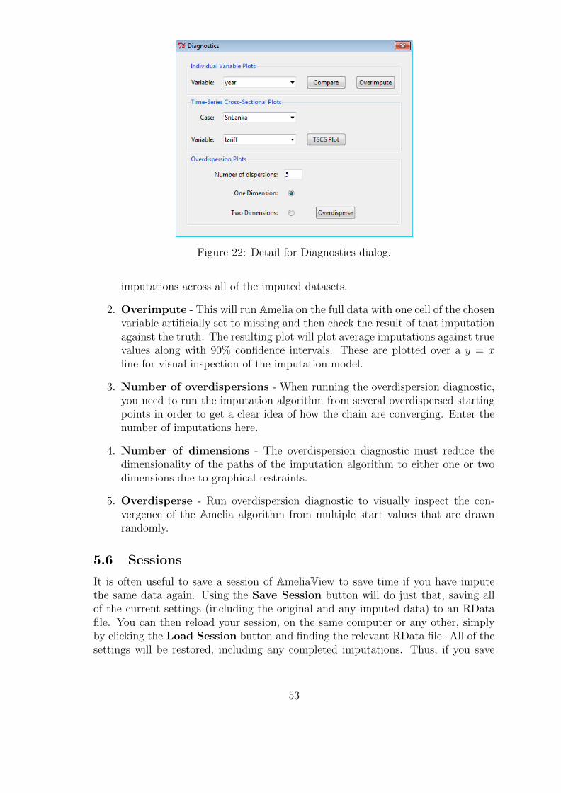
Figure 22: Detail for Diagnostics dialog.
imputations across all of the imputed datasets.
2. Overimpute - This will run Amelia on the full data with one cell of the chosenvariable artificially set to missing and then check the result of that imputationagainst the truth. The resulting plot will plot average imputations against truevalues along with 90% confidence intervals. These are plotted over a y = xline for visual inspection of the imputation model.
3. Number of overdispersions - When running the overdispersion diagnostic,you need to run the imputation algorithm from several overdispersed startingpoints in order to get a clear idea of how the chain are converging. Enter thenumber of imputations here.
4. Number of dimensions - The overdispersion diagnostic must reduce thedimensionality of the paths of the imputation algorithm to either one or twodimensions due to graphical restraints.
5. Overdisperse - Run overdispersion diagnostic to visually inspect the con-vergence of the Amelia algorithm from multiple start values that are drawnrandomly.
5.6 Sessions
It is often useful to save a session of AmeliaView to save time if you have imputethe same data again. Using the Save Session button will do just that, saving allof the current settings (including the original and any imputed data) to an RDatafile. You can then reload your session, on the same computer or any other, simplyby clicking the Load Session button and finding the relevant RData file. All of thesettings will be restored, including any completed imputations. Thus, if you save
53
the session after imputing, you can always load up those imputations and view theirdiagnostics using the sessions feature of AmeliaView.
References
Abayomi, Kobi, Andrew Gelman and Marc Levy. 2008. “Diagnostics for multivariateimputations.” Applied Statistics 57(3):273–291.
Dempster, Arthur P., N.M. Laird and D.B. Rubin. 1977. “Maximum likelihoodestimation from incomplete data via the em algorithm.” Journal of the RoyalStatistical Society B 39:1–38.
Honaker, James, Anne Joseph, Gary King, Kenneth Scheve and Nau-nihal Singh. 1998-2002. “AMELIA: A program for missing data.”.http://gking.harvard.edu/amelia.
Honaker, James and Gary King. 2010. “What to do about missing values in timeseries cross-section data.” American Journal of Political Science 54(2):561–581.http://gking.harvard.edu/files/abs/pr-abs.shtml.
King, Gary, James Honaker, Anne Joseph and Kenneth Scheve. 2001.“Analyzing incomplete political science data: An alternative algorithmfor multiple imputation.” American Political Science Review 95(1):49–69.http://gking.harvard.edu/files/abs/evil-abs.shtml.
King, Gary, Michael Tomz and Jason Wittenberg. 2000. “Making the most of sta-tistical analyses: Improving interpretation and presentation.” American Journalof Political Science 44(2):341–355. http://gking.harvard.edu/files/abs/making-abs.shtml.
Milner, Helen and Keiko Kubota. 2005. “Why the move to free trade? Democ-racy and trade policy in the developing countries.” International Organization59(1):107–143.
Schafer, Joseph L. 1997. Analysis of incomplete multivariate data. London: Chap-man & Hall.
Schafer, Joseph L. and Maren K. Olsen. 1998. “Multiple imputation for multivariatemissing-data problems: A data analyst’s perspective.” Multivariate BehavioralResearch 33(4):545–571.
54