Design-002 Revised: Oct 18, 2012

1

Ammonia Synthesis with Aspen Plus® V8.0

Part 2 Closed Loop Simulation of Ammonia Synthesis

1. Lesson Objectives Review Aspen Plus convergence methods

Build upon the open loop Ammonia Synthesis process simulation

Insert a purge stream

Learn how to close recycle loops

Explore closed loop convergence methods

Optimize process operating conditions to maximize product composition and flowrate

Learn how to utilize the model analysis tools built into Aspen Plus

Find the optimal purge fraction to meet desired product specifications

Determine the effect on product composition of a decrease in cooling efficiency of the pre -flash

cooling unit

2. Prerequisites Aspen Plus V8.0

Design-001 Module (Part 1 of this series)

3. Background; Recap of Ammonia Process

Design-002 Revised: Oct 18, 2012

2

The examples presented are solely intended to illustrate specific concepts and principles. They may not

reflect an industrial application or real situation.

4. Review of Aspen Plus Convergence Methods There are several methods Aspen Plus can utilize to converge recycle loops. Convergence in Aspen Plus is an

iterative process consisting of making guesses for tear streams and then comparing the calculated stream values

with the guessed values. If these values are equivalent within a certain tolerance, then the simulation h as

successfully converged. Consider the following example shown in the flowsheet below:

To calculate the properties of stream S4, the properties of stream S2 must be known or calculated. To calculate

the properties of stream S2, the properties of streams S1 and S4 must be known or calculated. In mathematical

terms we have:

( )

( )

The mutual dependency of streams S4 and S2 creates an algebraic loop. This loop can be removed by ‘tearing’ a

stream apart. For example, we can choose to hypothetically tear stream S4 into two separate streams. This

would result in the following flowsheet:

Design-002 Revised: Oct 18, 2012

3

Mathematically we now have the following:

( )

( )

There is no longer mutual dependency between streams S4 and S2. The issue now relies in finding a solution

that results in stream S5 being equal to stream S4. This is accomplished by utilizing iterative convergence

methods which are briefly described below. Based on the flowsheet you create, Aspen Plus will automatically

define tear streams to converge, or alternatively you can input user defined tear streams.

The following methods are available in Aspen Plus:

Direct substitution

Wegstein

Newton

Secant

Broyden

Sequential quadratic programming (SQP)

The direct substitution method is a slow but sure way to reach convergence. For each iteration, this method

uses the values calculated from the previous flowsheet pass as the new values of the tear stream. In

mathematical terms we have the following, where k is the iteration number.

( )

This sequence would be iterated until and are equivalent within a specified tolerance.

The Wegstein method is an extrapolation of the direct substitution method used to accelerate converge nce. It

attempts to estimate what the final solution will be based on the difference between successive iteration values.

This is the default convergence method for system generated tear convergence blocks and is usually the

quickest and most reliable method for tear stream convergence.

Newton’s convergence method for simultaneous nonlinear equations uses matrices of partial derivatives to

obtain a set of linear equations which are then solved. This process is iterated until convergence criteria are met.

Newton’s method requires the evaluation of the function and it’s derivative per iteration. This method provides

an efficient means of convergence only if a sufficiently good initial guess is provided. Use the Newton method

for tear streams only when the number of components is small or when convergence cannot be achieved by

other methods.

The secant method uses a succession of roots of secant lines to approximate the root of a function. Compared

with Newton’s method, the secant method does not require the evaluation of the functions derivative. This

enables this method to converge for systems involving non-elementary functions. The secant method can be

Design-002 Revised: Oct 18, 2012

4

used for converging single design specifications and is the default method in Aspen Plus for design specification

convergence.

Broyden’s method is a modification of the Newton and secant methods that uses approximate linearization

which can be extended to higher dimensions. This method is faster than Newton’s method but is often not as

reliable. Broyden’s method should be used to converge multiple tear streams or design specifications, and is

particularly useful when converging tear streams and design specifications simultaneously.

Sequential quadratic programming is an iterative method for flowsheet optimization. This method is useful for

simultaneous convergence of optimization problems with constraints and tear streams.

5. Aspen Plus Solution In Part 1 of this series (Design-001), the following flowsheet was developed for an open loop Ammonia Synthesis

process.

This process produces two outlet streams; a liquid stream containing the ammonia product and a vapor stream

containing mostly unreacted hydrogen and nitrogen. It is desired to capture and recycle these unreacted

materials to minimize costs and maximize product yield.

Add Recycle Loop to Ammonia Synthesis Process Beginning with the open loop flowsheet constructed in Part 1 of this series, a recycle loop will be constructed to

recover unreacted hydrogen and nitrogen contained in the vapor stream named OFFGAS, shown below.

Design-002 Revised: Oct 18, 2012

5

5.01. The first step will be to add a Splitter to separate the OFFGAS stream into two streams; a purge stream

and a recycle stream. As a rule of thumb, whenever a recycle stream exists, there must be an associated

purge stream to create an exit route for impurities or byproducts contained in the process. Often times

if an exit route does not exist, impurities will build up in the process and the simulation will fail to

converge due to a mass balance error.

5.02. On the main flowsheet add an FSplit block located in the Mixers/Splitters tab in the Model Palette. The

FSplit block will fractionally split a stream into several streams according to user specifications. Rename

this block S-100 and connect the OFFGAS stream to the inlet port. Construct two material outlet streams

and label one as the purge stream. This is shown below. Double click on the splitter block to specify the

split fraction. Enter a value of 0.01 for the Split fraction of the purge stream. This means that 1% of the

OFFGAS stream will be diverged to the purge stream.

Design-002 Revised: Oct 18, 2012

6

5.03. Next, we must add a compressor to bring the pressure of the recycle stream back up to the feed

conditions. Add a compressor (Compr) block from the Pressure Changers tab in the Model Palette.

Connect stream S7 to the inlet port and construct a material stream for the outlet port. Remember that

you can rotate and resize the block icons by right clicking the block and selecting either Rotate Icon or

Resize Icon.

5.04. Double click on the compressor block to specify the operating conditions. Select Isentropic as the Type

and enter a Discharge pressure of 271 atmospheres.

Design-002 Revised: Oct 18, 2012

7

5.05. The recycle stream is now ready to be connected back to the mixer block to close the loop. Right click on

the recycle stream, select Reconnect Destination, and connect the stream to the inlet port of the mixer

block. This can also be done by double clicking the arrow of the disconnected recycle stream. This

stream (S8) will be the tear stream in this simulation. Aspen Plus automatically recognizes and assigns

tear streams; however you can also specify which streams you would like to be tear streams.

5.06. Open the Control Panel and run the simulation (F5). You should result in an error stating that block C-

101 is not in mass balance and that the simulation failed to converge after 30 iterations.

Design-002 Revised: Oct 18, 2012

8

There are several steps you can take to overcome this issue. First, check to see which convergence

method is being used and check which stream is being converged. Scroll up to the very top of the

Control Panel.

Design-002 Revised: Oct 18, 2012

9

5.07. Aspen Plus is using the Wegstein method to converge recycle stream S8. The Wegstein method is a

good method to use when trying to converge a single recycle stream, and stream S8 is an appropriate

stream to attempt to converge. The next thing you can do is to check the maximum error per iteration

to see whether the solver is heading towards convergence or not. In the navigation pane, go to

Convergence | Convergence | $OLVER01 | Results. In the Summary tab you can see which variables

have converged and which haven’t after 30 iterations. Click the Tear History tab where you can view

the maximum error that occurs each iteration and which variable it occurs in. Click the Custom plot

button at the top of the screen.

Design-002 Revised: Oct 18, 2012

10

5.08. Select Iteration as the x-axis and Maximum error/Tolerance as the y-axis. Change the y-axis min to -

5000 and change the max to 5000. The plot should appear as below.

Design-002 Revised: Oct 18, 2012

11

5.09. By looking at the plot, it is clear that the Wegstein method is on the right track towards finding the

solution. It may be that the solver just needs a few more iterations to converge. In the navigation pane,

go to Convergence | Options | Methods. Click the Wegstein tab and increase the Maximum flowsheet

evaluations to 50. Run the simulation again. In the control panel you will see that the solver has now

converged after only 20 iterations. This is because the solver used the last calculation from the previous

run that failed to converge as the initial guess for the second run. If you reinitialize and run the

simulation again you will notice that the simulation converged after 49 iterations.

Design-002 Revised: Oct 18, 2012

12

5.10. Now that the simulation has converged, check the results. In the Home ribbon click Stream Summary

and then click Stream Table.

This will generate a stream table that will appear on the main flowsheet. Here you can see the flow and

composition of each stream.

Optimize the Purge Rate to Deliver Desired Product

5.11. We now wish determine the purge rate required to deliver a product with a mole fraction of 0.96

ammonia. First, check the composition of the current ammonia stream by clicking on the product stream

(LIQ-NH3) and clicking Stream Analysis | Composition in the Home ribbon. Select Mole for Composition

basis and press Go.

Design-002 Revised: Oct 18, 2012

13

From the composition analysis results, the mole fraction of ammonia in the product stream is only

0.955, which is below the specification of 0.96. We need to determine the purge rate required to reach

this product specification.

5.12. Go to the navigation pane and select Flowsheeting Options | Design Spec and click New. This will

create a design spec which we will use to vary the purge fraction in order to reach 0.96 mole fraction

ammonia in the product stream.

5.13. Under the Define tab select New. Enter the variable name NH3FRAC. A window will appear where you

must define the variable. Select Mole-Frac as type, LIQ-NH3 for Stream, and NH3 for Component.

Design-002 Revised: Oct 18, 2012

14

5.14. Next, move to the Spec tab and enter NH3FRAC for Spec, 0.96 as Target, and 0.0001 for Tolerance.

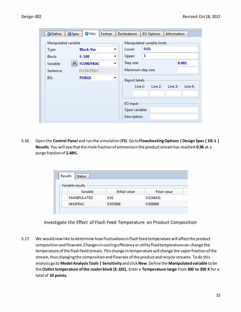
5.15. Move to the Vary tab and define the purge fraction from the splitter as the manipulated variable. Select

Block-Var for Type, S-100 for Block, FLOW/FRAC for Variable, and Purge for ID1. Enter 0.01 and 1 as the

Upper and Lower limits and a Step size of 0.001.

Design-002 Revised: Oct 18, 2012

15

5.16. Open the Control Panel and run the simulation (F5). Go to Flowsheeting Options | Design Spec | DS-1 |

Results. You will see that the mole fraction of ammonia in the product stream has reached 0.96 at a

purge fraction of 2.48%.

Investigate the Effect of Flash Feed Temperature on Product Composition

5.17. We would now like to determine how fluctuations in flash feed temperature will affect the product

composition and flowrate. Changes in cooling efficiency or utility fluid temperature can change the

temperature of the flash feed stream. This change in temperature will change the vapor fraction of the

stream, thus changing the composition and flowrate of the product and recycle streams. To do this

analysis go to Model Analysis Tools | Sensitivity and click New. Define the Manipulated variable to be

the Outlet temperature of the cooler block (E-101). Enter a Temperature range from 300 to 350 K for a

total of 10 points.

Design-002 Revised: Oct 18, 2012

16

5.18. In the Define tab, define the variables that you wish to measure, in this case ammonia mole fraction

and flowrate in the product stream.

5.19. In the Tabulate tab, select which variables you wish to view results for. Manually enter the variables

that you just created, or press the Fill variables button.

Design-002 Revised: Oct 18, 2012

17

5.20. Before running the simulation, be sure to deactivate the design spec we created in Flowsheeting

Options. This can be done by going to Flowsheeting Options and right clicking on the design spec and

selecting Deactivate. Once this is done, run the simulation. Check results by going to Model Analysis

Tools | Sensitivity | S-1 | Results. Click the Results Curve plot button on the Home ribbon. Select both

Mole fraction and Flowrate to plot against the varied parameter on the x-axis.

The results plot should look like the following.

Design-002 Revised: Oct 18, 2012

18

5.21. You will see that as temperature increases, both the product flowrate and product quality decrease,

which means that when operating this process it will be very important to monitor the flash feed

temperature in order to deliver high quality product.

6. Conclusion This simulation has proved the feasibility of this design by solving the mass and energy balances. It is now ready

to begin to analyze this process for its economic feasibility. See module Design-003 to being the economic

analysis.

Design-002 Revised: Oct 18, 2012

19

7. Copyright

Copyright © 2012 by Aspen Technology, Inc. (“AspenTech”). All rights reserved. This work may not be

reproduced or distributed in any form or by any means without the prior written consent of

AspenTech. ASPENTECH MAKES NO WARRANTY OR REPRESENTATION, EITHER EXPRESSED OR IMPLIED, WITH

RESPECT TO THIS WORK and assumes no liability for any errors or omissions. In no event will AspenTech be

liable to you for damages, including any loss of profits, lost savings, or other incidental or consequential

damages arising out of the use of the information contained in, or the digital files supplied with or for use with,

this work. This work and its contents are provided for educational purposes only.

AspenTech®, aspenONE®, and the Aspen leaf logo, are trademarks of Aspen Technology, Inc.. Brands and

product names mentioned in this documentation are trademarks or service marks of their respective companies.