AN ABSTRACT OF THE THESIS OF

Nichole I. Victory for the degree of Master of Science in Civil Engineering presented on June 13, 2007. Title: Quantification of Advection and Dispersion in Lateral Subsurface Flowpaths at the Hillslope-scale Abstract approved:

__________________________________________ Jonathan D. Istok

It is becoming increasingly important to understand fundamental hillslope-scale

hydrological processes. Most hillslope-sale transport experiments have generally

focused on conceptual findings or other aspect of flow behavior, rather than the

quantification of the mass transport mechanisms of advection and dispersion.

When the velocities have been quantified, dispersion has been mentioned as

present, but has not yet quantified. This study uses a natural gradient well-

injection tracer test to characterize solute transport in lateral subsurface

flowpaths. The breakthrough curves obtained from the tracer tests were analyzed

using traditional hillslope hydrology methods for calculating velocities, time to

peak and the Mosley [1982] method, as well as CXTFIT, a program that computes

average velocity and dispersion coefficients for breakthrough curves by fitting

experimental data to the 1-Dimensional convective-dispersion equation using a

non-linear least-squares regression technique.

Well injection tracer tests at the WS10 hillslope showed advection and dispersion

rates larger than reported from laboratory studies and comparable rates to those

reported from field studies. Lateral preferential flowpaths appeared to

significantly reduce travel time through the study hillslope. However, once tracer

was stored in the subsurface, the travel times and average velocities depended

largely on the applied driving force (i.e. intensity and duration of precipitation

and/or injection). The tracer tests also illustrated that as less tracer remained in

the flowpath the amount of water required to remove a quantity of mass

increased.

Through the quantification of advection and dispersion in Experiment 1, it was

shown not only that one flowpath had a larger advective velocity but also mixed

with the tracer-free water more due to it’s higher velocity. In addition, the

dispersion coefficients showed that while Inj1 and Inj2 have very similar BTCs,

Inj2’s dispersion coefficient was about twice that of Inj1’s, indicating that Inj2

spread longitudinally more than Inj1. Through the quantification of advection and

dispersion in Experiment 2, the large effect of stored water on apparent dispersion

was illustrated. As stored water plays a leading role in the hillslope hydrology,

accounting for the dispersion that results from storage is imperative to accurately

describing internal hillslope hydrological processes.

© Copyright by Nichole I. Victory June 13, 2007

All Rights Reserved

Quantification of Advection and Dispersion in Lateral Subsurface Flowpaths at the

Hillslope-scale

by Nichole I. Victory

A THESIS

submitted to

Oregon State University

in partial fulfillment of the requirements for the

degree of

Master of Science

Presented June 13, 2007

Commencement June 2008

Master of Science thesis of Nichole I. Victory presented on June 13, 2007. APPROVED: ______________________________________________________________ Major Professor, representing Civil Engineering ______________________________________________________________ Head of the Department of Civil, Construction and Environmental Engineering ______________________________________________________________ Dean of the Graduate School I understand that my thesis will become part of the permanent collection of Oregon State University libraries. My signature below authorizes release of my thesis to any reader upon request. ______________________________________________________________

Nichole I. Victory, Author

ACKNOWLEDGEMENTS

I wish to express my sincere thanks to the following people for their assistance.

Without their support this work would not have been possible.

Lukas Potts

Jesse Jones

Willem van Verseveld

Chris Graham

John Moreau

Kathy Keable

Jeff McDonnell

Jack Istok

And most of all, my family! My husband, Joe Dunn; my parents, Lynn and

Clarence Victory; and my brother, Mark Victory.

TABLE OF CONTENTS Page 1. INTRODUCTION .................................................................................1 2. SITE DESCRIPTION ............................................................................5 3. METHODS .........................................................................................7

3.1. Site and Experimental Set-up ...........................................................7 3.1.1. WS10 Well installations ...................................................................7 3.2. Two Tracer Experiments ................................................................10

3.2.1. Experiment One .....................................................................11 3.2.2. Experiment Two .....................................................................12

4.1. Experiment One............................................................................14 4.1.1. Inj1 in well E1 .......................................................................14 4.1.2. Inj2 in well C2 .......................................................................17 4.1.3. Flushes .................................................................................19

4.2. Experiment Two............................................................................22 5. DISCUSSION: CHARACTERIZATION OF LATERAL SUBSURFACE FLOW.....25

5.1. Advection and dispersion quantified in two flowpaths at the hillslope-scale: Experiment 1 ...............................................................................25 5.2. Advection and dispersion quantified in one flowpath under different flow conditions: Experiment 2 .................................................................29 5.3. Comparison of velocities and dispersivities with other studies.............32 5.4. Why quantify velocities and dispersivities? .......................................35

6. CONCLUSIONS ................................................................................37 BIBLIOGRAPHY ..........................................................................................38 APPENDICES .............................................................................................41

Appendix A: Dynamic Cone Penetrometer Profile .......................................42 Appendix B: Volume Equivalent Precipitation calculation .............................43 Appendix C: Determination of Mass recovered per well ...............................44 Appendix D: Theoretical concentration drop due to flowpath drop ................45

TABLE OF FIGURES

Figure Page 1: Study Site with trench, well locations and seep location indicated..................62: Well profile, (values in meters) ..................................................................83: BTC for Inj1 with evidence of additional concentration rise due to precipitation 2 days post-injection................................................................154: Inj1 calibration of in-situ field ISE (installed in the stilling basin) to the IC in the laboratory ........................................................................................175: BTC Inj2 with evidence of additional concentration rise due to a tracer-free water flush 2 days post-injection..................................................................186: Inj2 calibration of in-situ field ISE (installed in the stilling basin) to the IC in the laboratory ........................................................................................197: Cumulative mass recovered and cumulative water added (throughout the flushes) as a function of time from beginning of Inj1 ......................................208: CXTFIT results for calculated velocity and dispersion coefficient for the E1 flushes......................................................................................................219: CXTFIT results for calculated velocity and dispersion coefficient for the C2 flushes......................................................................................................2110: BTC for Inj3 showing injection and flush periods as well as the drops in volumetric flowrate and mass ratios during injection interruptions....................2311: Theoretical drop in concentration due to decrease flowpath volumetric flowrate and dilution from seep flow .............................................................2412: CXTFIT results for calculates of velocity and dispersion coefficient based on relative mass out of the trench during injection and flush phases of Inj3 ......2413: Initial BTCs Inj1 and Inj2 .....................................................................28

TABLE OF TABLES Table Page 1: Injection Summary................................................................................112: Injection parameters and breakthrough curve results ................................163: Summary of Velocities, Dispersion Coefficients and Dispersivities for Inj1, Inj2 and Inj3 .............................................................................................164: Assumptions by method (X indicates assumption satisfied).........................305: Velocities calculated from Experiments 1 and 2, Harr and McGuire for WS10 hillslope ...........................................................................................326: Empirical Values for unconsolidated porous media [Schnoor, 1996] .............357: CXTFIT calculated values from Experiments 1 and 2 ..................................35

LIST OF APPENDIX FIGURES

Figure Page 1: Dynamic Cone Penetrometer profile at well C2..........................................422: Dynamic Cone Penetrometer profile at well E1 ..........................................423: Flowchart of hillslope system with well injection ........................................46

Quantification of Advection and Dispersion in Lateral Subsurface Flowpaths at the Hillslope-scale

1. Introduction

Numerous studies have examined water transport through porous media in the

laboratory under controlled conditions [Brusseau, 1993; Hutchison et al, 2003;

Maraqa et al, 1997; Vanderborght, 2000, 2002] and in the field, under less

controlled conditions [Hewlett and Hibbert, 1963; Harr, 1977; Tsuboyama et al,

1994; Rodhe et al, 1996; Anderson et al, 1997; Nyberg et al, 1999]. Laboratory-

scale experiments have quantified how parameters vary with flow conditions (i.e.

unsaturated vs. saturated [Maraqa et al, 1997; Hutchison et al, 2003]), and

material properties (i.e., consolidated vs. non-consolidated). The quantitative

transport descriptions from such laboratory experiments have resulted from the

ability to create boundaries and homogeneous hydraulic properties, accurately

control boundary conditions and flowrates, isolate the system from outside

influences (i.e. precipitation, upslope drainage, etc.), and fully characterize the

porous media. Most importantly, the ability to manipulate one variable or

parameter while keeping all others constant has been an invaluable tool in the

laboratory for investigating transport mechanisms. In the field, attempts to

create boundaries and control boundary conditions have included the use of

barriers [Anderson, 1997; Brooks, 2004], cut-trenches [Mosley, 1982; Tsuboyama

et al, 1994], covered fields [Nyberg et al, 1999; Rodhe et al, 1996], and artificial

irrigation [Anderson et al, 1997; Tsuboyama et al, 1994]. Obviously, laboratory-

like control is not possible in the field. Hillslope-scale experiments aimed at

observing subsurface flow behavior have relied passively on natural precipitation

events [Harr, 1977; McGuire et al, 2007], the use of irrigators or sprinklers to

create “controlled” precipitation events [Tsuboyama et al, 1994; Anderson et al,

2

1997; Nyberg et al, 1999], and the tagging of water with tracers [Tsuboyama et

al, 1994; Anderson et al, 1997; McGuire et al, 2007].

While assessing a larger and therefore likely more representative area than found

in a laboratory, hillslope-scale experiments illustrate the degree of variability

inherent in the natural environment [Beven, 2006]. To date, mainly qualitative

descriptions of observed breakthrough curves (BTCs) and subsurface flow path

transport characteristics have been made at the hillslope-scale. This is due to the

difficulty in isolating a hillslope control volume in the field – necessary for

quantifying hillslope-scale flow and transport. Comparisons of laboratory and field

study results have revealed differences due to field-scale heterogeneity [Gelhar,

1992].

To better characterize the internal hydrologic processes and the effects of scale,

more field experiments are needed [Sidle, 2006]. These experiments not only

need to bridge the gap between laboratory and field scale observations [Gelhar,

1992], but also to bridge the gap between field observations and model

predictions [Beven, 2006]. Advection and dispersion, the major mechanisms in

mass transport processes [Schnoor, 1996], are important parameters to quantify

when observing the flow and transport of water through the subsurface. Many

field-based lateral subsurface flow studies at the hillslope-scale have reported

observed velocities, but have generally focused on conceptual findings or other

qualitative aspects of the flow behavior [Anderson et al, 1997; Nyberg et al,

1999; McGuire et al, 2007]. In addition, reported advective velocities include

time to peak [McGuire et al, 2007; Anderson et al, 1997], time to center of mass

(CoM) [Mosley, 1982], average, and Darcy [Harr, 1977] velocities. Often it is not

clear which velocity is reported as they are merely reported as “subsurface flow

3

velocities” [McGuire et al, 2007]. While some hillslope studies have “observed”

dispersion [Tsuboyama et al, 1994; Anderson et al, 1997; McGuire et al, 2007], or

the ramifications resulting from a lack of accounting for dispersion [Jones et al,

2006], no field-based hillslope-scale studies have calculated the amount of

dispersion from the BTCs observed.

The advection-dispersion equation (ADE) is used to describe solute transport and

accounts for the advective and dispersive components. The hydrodynamic

dispersion coefficient quantifies the amount of hydrodynamic dispersion or the

amount a solute spreads and is diluted in addition to its advective movement

[Bedient et al, 1997]. By fitting the ADE to an experimental BTC, using a non-

linear least-squares regression technique, the average velocity (advective) and

the hydrodynamic dispersion coefficient may be solved for simultaneously.

Dispersivity is a scaling value that relates a flowpaths average velocity to its

dispersion coefficient and is thought to be a characteristic of soil [Domenico &

Schwartz, 1998] as well as the scale observed [Schnoor, 1996; Gelhar, 1992].

The relationship between the dispersion coefficient and average velocity is linear

[Domenico & Schwartz, 1998] and dispersivities are calculated using the

equation:

Dα=v

(2)

where α is the dispersivity [m], D is the hydrodynamic dispersion coefficient

[m2/hr] , and v is the average (average pore-water) velocity [m/hr]. Dispersivity

is a constant based on location and is more easily used for comparison purposes

than D, which is dependent on the average velocity.

4

This study uses a natural gradient well-injection technique, used in groundwater

studies, to characterize and improve the understanding of lateral subsurface

flowpaths on a well-studied hillslope in the HJ Andrews (HJA) Experimental Forest,

Western Oregon, USA. The specific objectives of this study are to quantify

advective velocities and dispersion coefficients at the hillslope-scale and to use

the determined values to: 1) compare transport in two distinct flowpaths; 2)

compare transport in one flowpath under different injection conditions; 3)

compare to previous studies; and 4) discuss how these measurements may add to

the conceptualization of internal hillslope hydrological processes.

5

2. Site Description The HJA is located in the Willamette National Forest in the Oregon Cascade

Mountain Range. This study focused on a south-facing hillslope in a 10.2 ha

watershed known as Watershed 10 (WS10). The WS10 hillslope was extensively

studied by Harr [1977], and more recently by McGuire [2007]. The mean annual

precipitation at the site is 2350 mm, which falls mainly between October and

April, during low intensity, long-duration frontal storms [Harr, 1977]. While the

streamflow is perennial, flows are considerably higher during the winter wet-

season than the low base flow in the summer dry-season. Clear-cut in 1975,

WS10 is dominated by second growth Douglas-fir [Jones, 2000]. The elevation

ranges from 425 to 700 m. Due to the steep terrain (~48° near the stream), the

soils are shallow [Rothacher et al, 1967], ranging from 0.5 m at the lower

elevations to 5 m at the ridgeline [van Verseveld, unpublished data]. Ranken

[1974] analyzed 452 soil cores from 11 soil pits in WS10 and reported the mean

soil Ks (from Pit 3) decreased from 8.9 m/hr at 30 cm to 0.05 m/hr at 160 cm,

and often changed abruptly within the profile [Ranken, 1974]. Soil porosity

varied between 60-70% at the surface, and decreased to ~50% at depth

[Ranken, 1974]. Surface soils in WS10 are highly permeable, while sub-surface

soils are less permeable. The subsurface consists of saprolite underlain by rock

from pyroclastic flows [Ranken, 1974].

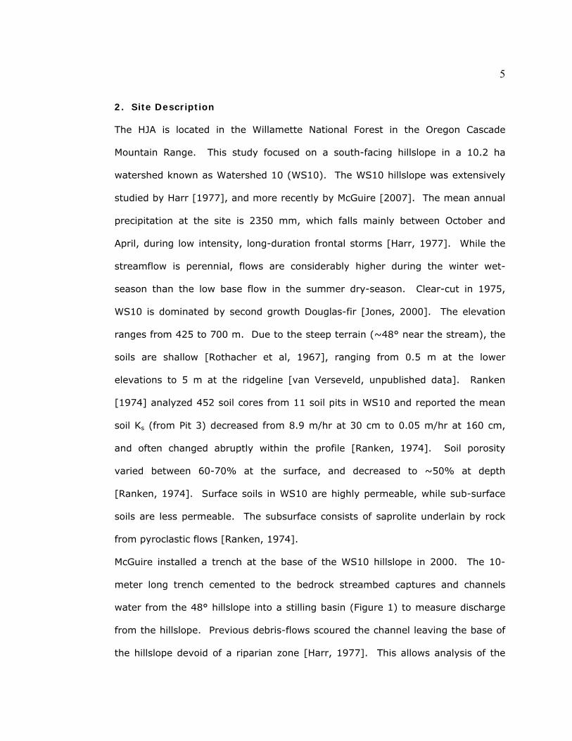
McGuire installed a trench at the base of the WS10 hillslope in 2000. The 10-

meter long trench cemented to the bedrock streambed captures and channels

water from the 48° hillslope into a stilling basin (Figure 1) to measure discharge

from the hillslope. Previous debris-flows scoured the channel leaving the base of

the hillslope devoid of a riparian zone [Harr, 1977]. This allows analysis of the

6

hillslope outflow without the influence of the riparian zone. At the upslope end of

the trench a seep continuously supplies water to the trench. The trench collects

lateral subsurface flow from the hillslope, except for the flow that may bypass the

trench (on either side) or deeply percolate into the bedrock. This seep may be

related to the presence of a north-northwesterly antidesitic, vertical dike that

manifests itself as a localized zone of saturated soil [Swanson and James, 1975;

Harr, 1977].

500

Well E1 Well C2 Stilling Basin

0 10 20 m Contour Interval 5m

490 N

Seep

Figure 1: Study Site with trench, well locations and seep location indicated

7

3. Methods

3.1. Site and Experimental Set-up

3.1.1. WS10 Well installations

A grid-like pattern of wells has been installed on the WS10 hillslope [van

Verseveld, unpublished data]. A hand-auger bored holes for the well installations.

Constructed of 3.8 cm O.D., 3.2 cm I.D. PVC pipe each of the wells are perforated

and screened over the bottom 20 cm. Dynamic cone penetrometer, Easting-

Northing, and elevation data [van Verseveld, unpublished data] are available for

each of the wells on the hill in WS10, as well as for the trench.

Two wells, C2 and E1 were used for the experiments (Figure 1). Well E1 is

located approximately 15 m upslope from the middle of the trench. The soil depth

at E1 is 1.23 m, while the well penetrates the top 0.81 m of soil (Figure 2).

Dynamic cone penetrometer data shows the resistance from the soil surface to the

well base is relatively constant and low (<20 knocks per 10 cm, Appendix A).

Below the E1 well base, the resistance increases sharply at two depths with a

region in between that has a relatively constant and low resistance, (97 and 120

m are where the resistance increases). At 0.81 m, the average total porosity is

approximately 0.62 and the soil Ks is approximately 6.6 m/hr [Ranken, 1974].

Well C2 is located approximately 9 m upslope from the middle of the trench. The

soil depth at C2 is 0.43 m, while C2 penetrates the top 0.35 m of soil, Figure 2.

The dynamic cone penetrometer data gathered at C2 illustrate that the resistance

from the soil surface to the well base is fairly constant and relatively low (<20

knocks per 10 cm), Appendix A). Below the C2 well base, the resistance

increases dramatically (over the next 40 cm) to the bedrock. At 0.35 m, the

8

average porosity is approximately 0.67, and the soil Ks is approximately 8.9 m/hr

[Ranken, 1974].

C2

0.038

0.038

E1

Ground surface

Bedrock

0.2

0.2

0.43

0.35

0.81

1.23

0.42

0.08

C2

0.038

0.038

E1

C2

0.038

C2

0.038

0.038

E1

0.0380.038

E1

Ground surface

Bedrock

0.2

0.2

0.20.2

0.20.2

0.43

0.35

0.81

1.23

0.43

0.35

0.43

0.35

0.81

1.23

0.81

1.23

0.42

0.08

0.420.42

0.080.08 Figure 2: Well profile, (values in meters)

3.1.2. Experimental Set-up

Tracer injections were performed in Wells E1 and C2. A Masterflex® precision

peristaltic pump (Cole Parmer Model# 7518-00) controlled the injection

volumetric flowrate (Qinj). Qinj was measured volumetrically by recording the time

required to pump 1L from the carboy, or by collecting a known volume of the

outflow from the injection line into a graduated cylinder. Injection solution was

pumped from a carboy into each well. Stream water was used for the tracer-free

9

water injections, while lithium bromide solutions were used for the tracer

injections.

Water collected in the trench is piped into a stilling basin where the residence time

varied between 0.13 and 12 minutes over the course of the experiments,

depending on the seep flow. Two capacitance rods (TruTrack, Model# WT-VO

500) measured water height and were used to calibrate the water level in the

basin to the volumetric flow rate of water through the v-notch weir. A bromide

ion-selective electrode (ISE) (Instrumentation Northwest) measured the

subsurface stormflow trench bromide concentration, [Br-]trench, as well as the air

and water temperatures in the stilling basin. Data was recorded using a CR10

datalogger (Campbell Scientific). To verify the accuracy of the ISE

measurements, grab samples were taken from the trench outflow during each of

the injections. Grab samples were also obtained from the seep during the

injections. All of the grab samples were analyzed in the laboratory using a D-120

Ion Chromatograph (IC) (Dionex, Sunnyvale, CA).

3.1.3. Calculations

Three methods were used to calculate subsurface lateral flow velocities: the time

to peak; time to center of mass (CoM) [Mosley, 1982]; and the CXTFIT method

[Toride, 1999]. The time to peak and the time to CoM methods, both define the

travel distance as the linear distance between the injection point and the

measurement point. The time to peak method defines the travel time as the time

to the peak of the BTC from the beginning of the injection. In the time to CoM

method, the mean travel time is defined as the time to the center of mass of the

BTC from the center of mass of the injection [Mosley, 1982]. CXTFIT 2.1 is a one-

dimensional analytical model that uses a non-linear least-squares regression with

10

the ADE to fit transport parameters (velocities and dispersion coefficients) to

tracer data [Toride, 1999]. The cumulative mass recovered was used in relation

to the total mass recovered in order to analyze the behavior of the tracer

recovered, not the tracer that became stored in the subsurface. To do this we

used the ratio:

cumulative mass recovered at time ttotal mass recovered

where t refers to the time from the beginning of tracer injection to normalize the

concentration data for input into CXTFIT. Solutions fitted to experimental results

based on the ADE allow parameters (e.g. average pore-water velocity and

dispersion coefficient) to be quantified [Toride et al, 1999].

3.2. Two Tracer Experiments

Two tracer experiments were conducted between April 12 and June 20, 2006. The

first experiment, Experiment 1, consisted of a one hour pulse tracer injection, into

each well (well E1 and well C2), followed by a series of tracer-free water flushes.

The flushing of the wells with tracer-free water continued until the second

experiment, Experiment 2, began. Experiment 2 began on June 18, 2006 and

lasted for three days. Experiment 2 consisted of a longer, eight-hour pulse tracer

injection into Well C2 (Table 1). The three injections consisted of three phases:

1) pre-saturation, 2) tracer injection, and 3) tracer-free water flush. The pre-

saturation phase consisted of a tracer-free water injection to wet up the flow path

between the well and the stream, to minimize interference from the unsaturated

zone. Immediately following the pre-saturation phase, the tracer injection began

with the same Qinj as the pre-saturation phase to access the same flow path

11

established during the pre-saturation phase. The flush phase immediately

followed the tracer injection with the same Qinj as the previous phases.

Table 1: Injection Summary Inj1 Inj2 Inj3 Well ID E1 C2 C2 Upslope Distance from Trench (m) 15.2 8.9 8.9 Qinj (L/hr) 3 2 18 Qtrench (L/hr) 76 206 46 Qinj as % of Qtrench 4 1 39 Input Tracer Concentration (mg Br-/L) 123,000 123,000 113 Mass Injection rate (mg/hr) 369,000 246,000 2034 Length of Injection (hr) 1 1 8.2

3.2.1. Experiment One

Experiment 1 included two pulse tracer injections, Injection 1 (Inj1) and Injection

2 (Inj2), as well as a series of 27 flushes. Both Inj1 and Inj2 were short duration,

high concentration pulse injections with low Qinj (Table 1). The Qinj‘s for

Experiment 1 were assumed to represent the average precipitation intensity of 3

mm/hr. The rates accounted for the size of the well and an assumed spreading of

injected water 0.5 m on either side of the well. A tracer concentration of 123,000

mg Br-/L was used for both Inj1 and Inj2 to ensure an observable concentration.

3.2.1.1. Injection 1

Inj1 was performed on April 12, 2006 in well E1. During Inj1, the Qinj was kept

constant at 3 L/hr. Tracer-free water was injected for three hours to pre-saturate

the flow path. Immediately following the pre-saturation, a tracer solution of

123,000mg Br-/L was injected at 3 L/hr for one hour (introducing a total of

369,000 mg Br- into the subsurface). A 1.5 hrs tracer-free water flush

immediately followed the tracer injection. Two days after Inj1, the movement of

tracer was augmented by a rain storm, Storm1.

12

3.2.1.2. Injection 2

Well C2 was used for the second injection on April 19, 2006. Due to C2’s shorter

upslope distance from the trench a lower Qinj (2 L/hr) was used. Tracer-free

water was injected for 1.5 hrs to pre-saturate the flow path, followed by a tracer

injection of 123,000mg Br-/L, which introduced a total of 246,000 mg Br- into the

subsurface. A two hour tracer-free water flush immediately followed the tracer

injection. Two days later well C2 received an additional tracer-free water flush,

Flush1.

3.2.1.3. Flushes

After Storm1 and Flush1, it was deemed necessary to continue flushing the wells

with tracer-free water. The objectives of the flushing were twofold: 1) to remove

the bromide tracer from the flow path and 2) to observe the behavior of the tracer

in the flow path under various conditions of antecedent wetness and injection

rates. A total of 27 flushes were performed on both wells C2 and E1.

3.2.2. Experiment Two

On June 18, Experiment 2 began with a steady-state well injection, Inj3. The Qinj

(18 L/hr) for Experiment 2 was based on the observed build-up of water in the

injection well, so as not to exceed the screened portion of the well. Tracer-free

water was injected for five hours on the night of June 17 and 1.75 hours on the

morning of the 18th to pre-saturate the flow path. A notable shift (~18.5 L/hr) in

Qtrench that was approximately equal to Qinj (~18 L/hr) signified the completion of

the pre-saturation phase. Immediately following the pre-saturation phase, a

tracer solution of 115 mg Br-/L was injected for 8.2 hours (Table 1) until technical

difficulties temporarily prevented further injection. The tracer concentration was

selected to minimize the buoyancy-induced effects that could occur due to the

13

density difference between the tracer and the water already present in the system

[Istok and Humphrey, 1995]. After 1.5 hours with no injection, an 8-hour tracer-

free water flush began. The flushing was interrupted again for 2.75 hours,

followed by an additional 24.5 hrs of flushing, with the exception of another 4.25

hr interruption. The interruptions were due to technical issues with the pumping

system.

In Experiment 2, tracer was pushed out of the flowpath using an immediate and

equal magnitude flush, rather than an injection followed by a long period of

intermittent flush and drainage cycles. The flushing phase of Experiment 2 lasted

for two days.

14

4. Results

4.1. Experiment One

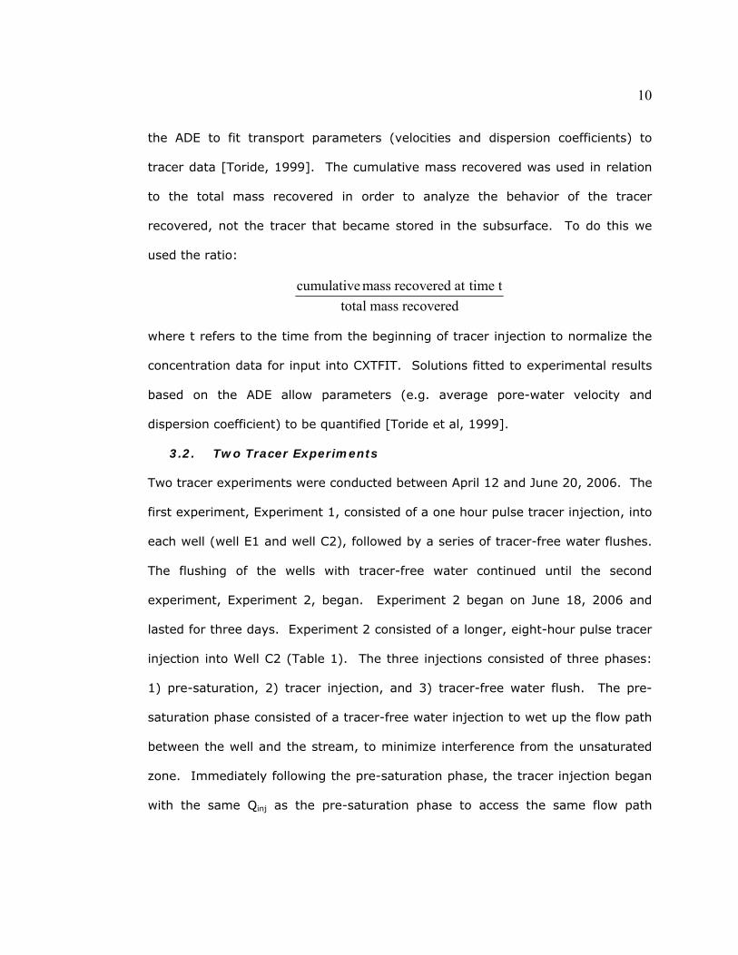
4.1.1. Inj1 in well E1 Inj1 produced a BTC typical of a pulse tracer injection, with a short duration [Br-

]trench peak in relation to the long duration of the BTC (Figure 3). Some of the

early concentration data are missing due to the ISE being calibrated with standard

solutions during the beginning of the experiment. The [Br-]trench from Inj1 peaked

around 80 mg Br-/L, after the injection ceased. During Inj1 and its initial BTC (i.e.

the first rise and fall in measured concentration), Qtrench remained relatively

constant. Inj1’s contribution to Qtrench was minimal accounting for approximately

4% of Qtrench (Table 1). During the 48 hours immediately following Inj1, 13% of

the injected tracer was recovered (Table 2). While a 5 mm rainstorm that

occurred about 23 hours after Inj1 had little effect on the [Br-]trench, a larger 39.5

mm rainstorm, two days after Inj1 caused an increase in the [Br-]trench, suggesting

that the storm mobilized some of the tracer remaining. After the first 25 mm of

precipitation was added during the second rainstorm, Qtrench increased

dramatically and diluted the [Br-]trench. While not shown, the mass flowrate

increased with the increased Qtrench. The time to peak method yielded an average

velocity of 4.45 m/hr (Table 3). Using the time to CoM method for the 48 hours

immediately following Inj1, the average velocity was 1.1 m/hr (Table 3). CXTFIT

was not used to calculate a velocity for Inj1.

15

0

0.2

0.4

Pre

cipitation (

mm

)

0

25

50

75

100

0 0.5 1 1.5 2 2.5 3Days from beginning of injection

[Br- ] t

ren

ch (

mg

Br- /

L)

0

60

120

180

240

Qtr

en

ch (

L/

hr)

Tracer-free water injectionTracer injection[Br-]Q

Figure 3: BTC for Inj1 with evidence of additional concentration rise due to precipitation 2 days post-injection

16

Table 2: Injection parameters and breakthrough curve results Inj1 Inj2 Inj3 Well ID E1 C2 C2 Upslope Distance from Trench (m) 15.2 8.9 8.9 Qinj (L/hr) 3 2 18 Qtrench (L/hr) 76 206 46 Qinj as % of Qtrench 4 1 39 Input Tracer Concentration (mg Br-/L) 123,000 123,000 113 Mass Injection rate (mg/hr) 369,000 246,000 2034 % Recovery during injection 13 18 ~90 Overall % mass recovered 64 >90 Center of Mass of Bromide (hrs) 10.5 14.5 8 Average velocity (m/hr) [Time to CoM] 1.45 0.63 1.13 Max. velocity (m/hr) [Mosley, 1982] 15.2 7 10.7 % Qinj measured at trench 0 0 ~100 Peak [Br-]trench (mg Br-/L) 80.6 23 27 Peak Qtrench (L/hr) 81.2 177 65.5 Peak Mass Flow (mg/hr) 11100 3325 1767 CoM input to Conc. Peak (min.) 175 230 260 Minutes from End of tracer to Conc. Peak 145 200 15 Minutes from End of Flush to Conc. Peak 60 75 N/A

Table 3: Summary of Velocities, Dispersion Coefficients and Dispersivities for Inj1, Inj2 and Inj3

Time to peak Mosley Velocity, v (m hr-1)

Dispersion coefficient, D (m2 hr-1)

Dispersivity, α (m)

Inj1 (E1) 4.45 1.12Inj2 (C2) 2.05 0.57E1 flushes 0.00029 0.020 1.6 83C2 flushes 0.00015 0.006 0.76 127

Inj3 (overall) 1.08 0.62 0.78 1.7 2.2

CXTFIT

Velocity, v (m hr-1)

[Br-]trench measurements from the field ISE agreed with the measurements made

using the laboratory IC (Figure 4 inset). However, the grab samples taken from

the seep, at the upper end of the trench, diverged from the trench samples:

increasing more rapidly and reaching much higher concentrations (Figure 4). This

seep response indicated that E1’s flowpath to the trench intersected the seep.

17

The [Br-]trench is less than that at the seep due to dilution by water entering the

trench through a pathway other than the seep.

0

25

50

75

100

125

150

175

200

14:00 16:00 18:00 20:00Time on April 12, 2006 (hr:min)

[Br- ]

(mg

Br- /

L) IC [Br-]

ISE [Br-]

IC [Br-] @ Seep

y= 0.8994x + 0.7006R2= 0.9908

0

20

40

60

0 20 40IC (mg Br-/L)

ISE (

mg

Br- /

L)

60

Figure 4: Inj1 calibration of in-situ field ISE (installed in the stilling basin) to the IC in the laboratory

4.1.2. Inj2 in well C2

Inj2’s pulse tracer injection also produced a short-lived [Br-]trench peak, post-

injection (Figure 5). The [Br-]trench from Inj2 peaked around 23 mg Br-/L. Inj2’s

contribution to Qtrench was miniscule, accounting for approximately 1% of Qtrench.

Qtrench decreased throughout Inj2 and its initial BTC. A small 1.25 mm

precipitation event about 32 hours after Inj2 was not large enough to mobilize

tracer remaining in either E1 or C2’s flowpath. However, two days after Inj2 a

tracer-free water flush into C2 mobilized some of the tracer causing a second

18

increase in the [Br-]trench, which peaked after the tracer-free water flush ceased.

The time to peak method yielded an average velocity of 2.05 m/hr (Table 3).

Using the time to CoM method for the 48 hours immediately following Inj2, the

average velocity was 0.57 m/hr (Table 3). CXTFIT was not used to calculate a

velocity for Inj2.

0

0.2

0.4

Prec

ipitat

ion (m

m)

0

25

50

75

100

0 0.5 1 1.5 2 2.5 3Days from beginning of injection

[Br- ] t

ren

ch (

mg

Br- /

L)

0

60

120

180

240

Qtr

en

ch (

L/

hr)

Tracer-free water injectionTracer injection[Br-]Q

Figure 5: BTC Inj2 with evidence of additional concentration rise due to a tracer-free water flush 2 days post-injection

19

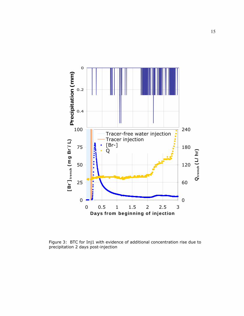
The field ISE measurements agreed with the IC measurements (Figure 6 inset).

The grab samples taken from the seep at the upper end of the trench were

measured using the laboratory IC and did not track the [Br-]trench measurements.

The [Br-]seep did not increase during Inj2, Figure 6. Unlike E1 (Inj1), C2’s flowpath

did not appear to intersect the seep.

0

5

10

15

20

25

12:45 14:45 16:45 18:45Time on April 19, 2006 (hr:min)

[Br- ]

(mg

Br- /

L)

IC [Br-]

ISE [Br-]

IC [Br-] @ Seep

y= 1.1089x + 0.6877R2= 0.9907

0

20

40

60

0 20 40IC (mg Br-/L)

ISE (

mg

Br- /

L)

60

Figure 6: Inj2 calibration of in-situ field ISE (installed in the stilling basin) to the IC in the laboratory

4.1.3. Flushes

Figure 7 illustrates the percent of cumulative mass recovered during Experiment

1, from both wells with time from the beginning of Inj1, as well as the percent of

cumulative water added to the system by both precipitation and flushing. The

volume of water injected and volume equivalent precipitation (see Appendix B)

were combined to couple the water added to the system into a single, cumulative

20

water parameter. Over sixty percent of the recovered mass was recovered within

the first 400 hours, during which time only 20% of the cumulative water had been

added.

0

0.2

0.4

0.6

0.8

1

1.2

0 500 1000 1500

Time from beginning Inj1 (hrs)

% m

ass

reco

vere

d a

nd

% w

ate

r ad

ded

% mass recoveredcumulative water added

Figure 7: Cumulative mass recovered and cumulative water added (throughout the flushes) as a function of time from beginning of Inj1

Separate CXTFIT least-squares regressions were conducted for the E1 flushes and

C2 flushes (Figures 8 and 9). CXTFIT calculated velocities of 0.02 and 0.006

m/hr, and dispersion coefficients of 1.6 and 0.76 m2/hr for E1 and C2,

respectively (Table 3).

21

0

0.2

0.4

0.6

0.8

1

1.2

0 20000 40000 60000 80000 100000

Time from beginning of Inj1 (min.)

Mass

reco

vere

d/

tota

l m

ass

re

covere

dObsFitted

R2= 0.851MSE= 0.0059

Figure 8: CXTFIT results for calculated velocity and dispersion coefficient for the E1 flushes

0

0.2

0.4

0.6

0.8

1

1.2

0 20000 40000 60000 80000 100000

Time from beginning of Inj2 (min.)

Mass

reco

vere

d/

tota

l m

ass

re

covere

d

ObsFitted

R2= 0.892MSE= 0.0056

Figure 9: CXTFIT results for calculated velocity and dispersion coefficient for the C2 flushes

22

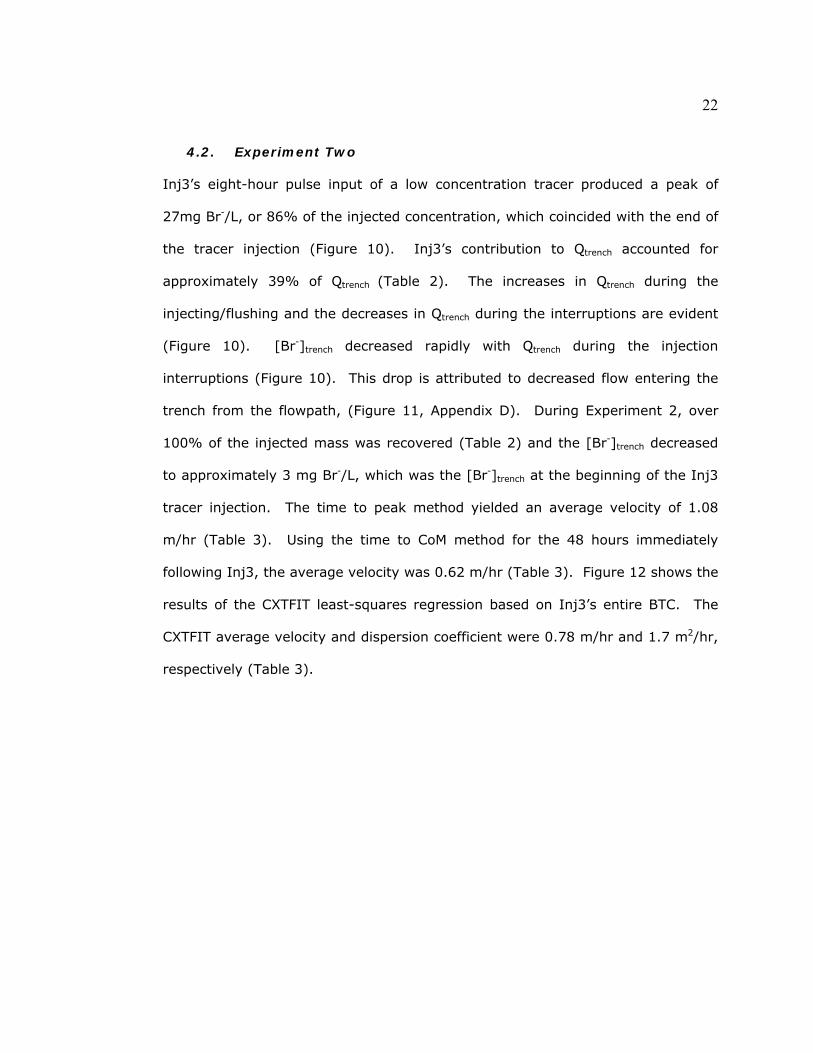
4.2. Experiment Two Inj3 h of a low concentration tracer produced a peak of ’s eig t-hour pulse input

27mg Br-/L, or 86% of the injected concentration, which coincided with the end of

the tracer injection (Figure 10). Inj3’s contribution to Qtrench accounted for

approximately 39% of Qtrench (Table 2). The increases in Qtrench during the

injecting/flushing and the decreases in Qtrench during the interruptions are evident

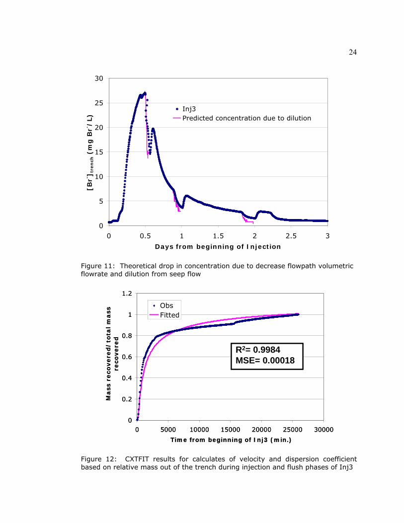
(Figure 10). [Br-]trench decreased rapidly with Qtrench during the injection

interruptions (Figure 10). This drop is attributed to decreased flow entering the

trench from the flowpath, (Figure 11, Appendix D). During Experiment 2, over

100% of the injected mass was recovered (Table 2) and the [Br-]trench decreased

to approximately 3 mg Br-/L, which was the [Br-]trench at the beginning of the Inj3

tracer injection. The time to peak method yielded an average velocity of 1.08

m/hr (Table 3). Using the time to CoM method for the 48 hours immediately

following Inj3, the average velocity was 0.62 m/hr (Table 3). Figure 12 shows the

results of the CXTFIT least-squares regression based on Inj3’s entire BTC. The

CXTFIT average velocity and dispersion coefficient were 0.78 m/hr and 1.7 m2/hr,

respectively (Table 3).

23

0

0.2

0.4

0.6

0.8

1

0 0.5 1 1.5 2 2.5 3Days from beginning of Inj3

Mass

eff

luen

t/M

ass

In

j.

0

50

100

150

200

250

Q (

L/

hr)

Tracer-free waterTracerInj3Q

Figure 10: BTC for Inj3 showing injection and flush periods as well as the drops in volumetric flowrate and mass ratios during injection interruptions

24

0

5

10

15

20

25

30

0 0.5 1 1.5 2 2.5

Days from beginning of Injection

[Br- ] t

ren

ch (

mg

Br- /

L)

3

Inj3Predicted concentration due to dilution

Figure 11: Theoretical drop in concentration due to decrease flowpath volumetric flowrate and dilution from seep flow

0

0.2

0.4

0.6

0.8

1

1.2

0 5000 10000 15000 20000 25000 30000

Time from beginning of Inj3 (min.)

Mass

reco

vere

d/

tota

l m

ass

re

covere

d

ObsFitted

R2= 0.9984MSE= 0.00018

0

0.2

0.4

0.6

0.8

1

1.2

0 5000 10000 15000 20000 25000 30000

Time from beginning of Inj3 (min.)

Mass

reco

vere

d/

tota

l m

ass

re

covere

d

ObsFitted

R2= 0.9984MSE= 0.00018

Figure 12: CXTFIT results for calculates of velocity and dispersion coefficient based on relative mass out of the trench during injection and flush phases of Inj3

25

5. Discussion: Characterization of lateral subsurface flow

To date, field-based hillslope hydrology studies have not quantified dispersion.

While hillslope studies that have calculated velocities (i.e. the advective

mechanism of transport) often observe evidence of dispersion, the accompanying

discussions have tended to focus on other aspects of the observed responses (i.e.

transit times and other directional transport issues [McGuire et al, 2007;

Anderson et al, 1997; Tsuboyama et al, 1994]). As a result, we still do not know

the effect of dispersion on the observed responses. However, due to the high

velocities and additional preferential flowpaths, dispersion at the hillslope-scale

should be larger than dispersion at the laboratory-scale and in groundwater

systems.

Well injection tracer tests at the WS10 hillslope showed advection and dispersion

rates larger than those reported from laboratory studies. Lateral preferential

flowpaths appeared to significantly reduce travel time through the study hillslope.

However, once tracer was stored in the subsurface, the travel times and average

velocities depended largely on the hydraulic gradient (i.e. intensity and duration

of precipitation and/or injection). The tracer tests also illustrated that as less

tracer remained in the flowpath the amount of water required to remove the same

quantity of tracer mass increased. These observed behaviors assist in the

explanation of the calculated velocities and dispersivities and how they relate to

fundamental hillslope hydrological processes.

5.1. Advection and dispersion quantified in two flowpaths at the hillslope-scale: Experiment 1

The quantification of advection and dispersion was complicated by a limited ability

to control field conditions and by differences in flowpath characteristics. By using

similar injection schemes in two wells, it was possible to compare different

26

methods for quantifying average velocities as well as investigate the dispersive

component of transport. Time to peak calculations, based on Inj1 and Inj2

indicated that E1’s velocity is nearly two times that of C2’s. During a steady-state

constant irrigation rate experiment [Anderson, 1997], where the peak was not

caused by a decrease in the hydraulic gradient, the time to peak method

accurately calculated the saturated subsurface flow velocities. The time to peak

method was invalid for determining velocities for Inj1 and Inj2, since the times to

peak during Inj1 and Inj2 were artifacts of a decreased hydraulic gradient. The

decrease in the hydraulic gradient caused the peak to occur earlier than it would

have under a constant hydraulic gradient, which resulted in larger apparent

average velocities than actual.

The time to CoM method’s reliance on the center of mass rather than the peak

shifts the timing into the tail of the BTC. The time to CoM velocities are nearly

one quarter of the time to peak velocities calculated from the initial BTC. The

time to CoM velocities for Inj1 and Inj2 represent the average velocities for

approximately 15% of the tracer, since the initial BTCs accounted for 15% of the

total mass injected (12% from E1 and 16% from C2). 85% of the tracer that

remained in the subsurface after Inj1 moved slower than the time to CoM

velocities. Noting the low mass recovery, the time to CoM method was repeated

to include the entire length of the flushes, Table 3. While 3-4 orders of magnitude

lower than the time to CoM estimates from Inj1 and Inj2, the smaller velocities

are an estimate for the long-term average velocity of the tracer recovered from

the flowpaths. The velocities were highly variable during the series of flushes,

with long draining cycles followed by brief injections. The long-term average

velocity of the water through the flowpath includes periods of flow where

27

velocities were larger and smaller (near zero). The small long-term average

velocities are indicative of long subsurface residence times. Both of the time to

CoM calculations indicated that E1’s velocity was nearly two times that of C2’s,

which agrees with the time to peak calculations as well as the observance of E1’s

connection to the seep. While both the time to peak and time to CoM methods

quantify the advective portion of transport, neither account for the dispersive

transport.

The CXTFIT average velocity for the E1 flushes was higher (~three times) than

that for C2 flushes and two orders of magnitude larger than the time to CoM

velocities for the E1 and C2 flushes, even with the same time intervals and the

same mass recoveries. The time to CoM method is entirely dependent on the

timing of the center of mass; however, tailing in the BTC caused by dispersion

skews the timing to the right of the center of mass and decreases the calculated

velocity. The dependence of the time to CoM method on a minimally disperse

BTC, may make it a weak choice for accurately determining hillslope-scale

advection. By simultaneously fitting both parameters to the observed transport

and minimizing the error, CXTFIT may estimate the long-term average velocity

and dispersion coefficient with more accuracy.

Figure 13 shows the BTCs of Inj1 and Inj2 with a normalized mass flowrate vs.

time from beginning of tracer injection. By looking at the BTCs in relation to each

other, it is difficult to conclude whether E1 or C2 exhibited more dispersion.

However, the tailing on the BTCs indicates that dispersion occurred [Domenico

and Schwartz, 2005; Schnoor, 1996]. Dispersion is difficult to discern from mere

observation of the BTCs and requires a more intensive analysis. E1’s dispersion

coefficient calculated by CXTFIT is nearly twice that of C2’s, indicating that the

28

solute spreads more in E1’s flowpath than it does in C2’s flowpath, which was not

evident through visual inspection of the BTCs. Since ~90% of the mass was

recovered from E1, the E1 dispersion results are probably more reliable than

those from C2, where only 46% of the mass was recovered, even though the r2

value from E1’s fit (r2= 0.851) is smaller than C2’s (r2= 0.892).

0

0.01

0.02

0.03

0.04

0.05

0.06

0 10 20 30 40Time from beginning of tracer injection (hrs)

Rela

tive M

ass

Flo

w (

m/

min

j)

50

Inj1 (E1) Inj2 (C2)

Figure 13: Initial BTCs Inj1 and Inj2

The dispersivity of E1’s flowpath is smaller than that of C2’s, meaning that for a

given average velocity, E1 would have less spreading than C2. E1’s flowpath is

expected to have less spreading because the preferential flow path seen in E1

intersects the seep and delivers the tracer to the trench more efficiently. The

water and tracer are able to travel in a more direct, less tortuous path, which

results in less dispersion because there is less influence from the porous media.

29

While the flushes mimic what may be seen during a series of natural precipitation

events, the cyclical pattern of flushing and draining during Experiment 1 created

the appearance of dispersion due to the stored water rather than depicting the

range of velocities. The water and tracer became stored in the soil due to either

capillarity or the presence of a lens, probably not due to sorption, since bromide is

a conservative tracer. This storage increased the transit time of the bulk of the

tracer due to the intermittent release of tracer. The increase in transit time due to

storage is a secondary mechanism (in addition to numerous and tortuous

flowpaths) for causing dispersion [Schnoor, 1996].

5.2. Advection and dispersion quantified in one flowpath under different flow conditions: Experiment 2

Each of the three methods used for velocity calculations in this study have

assumptions built in. The time to peak method relies on a high mass recovery

coupled with a constant velocity (i.e. a constant hydraulic gradient) to ensure

accurate estimates of velocity. The time to CoM method relies on a high mass

recovery alone. CXTFIT has the most assumptions including high mass recovery;

constant velocity (i.e. constant hydraulic gradient); one-dimensional transport;

homogeneous soil; no retardation; and no sorption. While it is important to

understand the assumptions implicit in calculations, it is difficult to satisfy all

assumptions for a calculation. By conducting Experiment 2 on C2’s flowpath it is

possible to compare the responses observed from two injection scenarios and

compare the results of the calculation methods when different assumptions are

not satisfied (Table 4). Velocities, dispersion coefficients and dispersivities for

Inj3 are shown in Table 3.

30

Table 4: Assumptions by method (X indicates assumption satisfied)

Method Assumption Inj1 Inj2 Inj3

High mass recovery X Time to Peak Constant velocity X Time to CoM

High mass recovery X

High mass recovery X

Constant velocity X

One-dimensional flow X X

Homogeneous

No retardation X X X

CXTFIT

No sorption X X X

The time to peak velocity calculated for Inj3 was 50% of that calculated for the

same flowpath during Inj2. The discrepancy in calculated velocities and their

divergence from the other velocities calculated, illustrates the effect of using the

time to peak method for calculating velocities when the assumptions implicit in

the theory are not satisfied (Table 4). Since Inj3 had a near constant hydraulic

gradient, it was expected to have reached its peak earlier and have a higher

velocity. However, since Inj2’s peak was artificially induced the time to peak

method resulted in an erroneously calculated velocity.

While the time to peak velocities of Inj2 and Inj3 differ by a factor of two, the

time to CoM velocities for Inj2 and Inj3 were nearly the same. This similarity

suggests that the time to CoM method may be valid for individual BTCs and short-

term velocity calculations, regardless of the mass recovery (Table 4). As seen in

the velocities calculated from the flushes, the long-term average velocity of

transport through a flowpath is considerably smaller than the short-term velocity

due to the fluctuations in the hydraulic gradient. Inj3’s calculated time to peak

31

velocity was closer to its time to CoM velocity than Inj2’s because Inj3 was closer

to the ideal scenario (Table 4) for using the time to peak method.

The CXTFIT average velocity was in between Inj3’s time to peak and time to CoM

velocities, though all three were relatively close with the smallest velocity equal to

over 60% of the largest. The CXTFIT average velocity is two orders of magnitude

larger for Inj3 than it is for the C2 flushes. CXTFIT’s constant velocity assumption

while grossly violated during Inj2, was a valid assumption during Inj3 (Table 4).

The Inj3 dispersion coefficient is over two times larger than the C2 flush

dispersion coefficient (Table 3). Since the dispersion coefficient is directly related

to the velocity [Schnoor, 1996], the dispersion coefficient from Inj3 being larger

than from the C2 flushes is expected.

The dispersivity for Inj3 is two orders of magnitude smaller than that for the C2

flushes. This disparity in dispersivities is partially due to the difference in

saturation level of the flowpath. Maraqa et al, [1997; Hutchison et al, 2003]

found that a dispersivity calculated from measurements in unsaturated soils is

higher than that calculated from measurements in a saturated or nearly saturated

soil. Since storage during draining periods (i.e. those with a decreasing or non-

existent hydraulic gradient) increases the apparent dispersion, the dispersion

coefficient calculated from the flushes is likely overestimated. In addition, the

advective movement of the tracer downslope occurs mainly during flushing, when

a hydraulic gradient is present. However, CXTFIT assumes a constant velocity,

which averages the short periods, when there is a higher lateral velocity, and long

periods, when there is a minimal lateral velocity probably underestimating the

effective advective movement. The likely overestimate of the dispersion

32

coefficient coupled with the likely underestimate of velocity, likely results in an

overestimate of dispersivity.

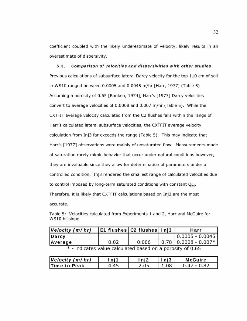
5.3. Comparison of velocities and dispersivities with other studies

Previous calculations of subsurface lateral Darcy velocity for the top 110 cm of soil

in WS10 ranged between 0.0005 and 0.0045 m/hr [Harr, 1977] (Table 5)

Assuming a porosity of 0.65 [Ranken, 1974], Harr’s [1977] Darcy velocities

convert to average velocities of 0.0008 and 0.007 m/hr (Table 5). While the

CXTFIT average velocity calculated from the C2 flushes falls within the range of

Harr’s calculated lateral subsurface velocities, the CXTFIT average velocity

calculation from Inj3 far exceeds the range (Table 5). This may indicate that

Harr’s [1977] observations were mainly of unsaturated flow. Measurements made

at saturation rarely mimic behavior that occur under natural conditions however,

they are invaluable since they allow for determination of parameters under a

controlled condition. Inj3 rendered the smallest range of calculated velocities due

to control imposed by long-term saturated conditions with constant Qinj.

Therefore, it is likely that CXTFIT calculations based on Inj3 are the most

accurate.

Table 5: Velocities calculated from Experiments 1 and 2, Harr and McGuire for WS10 hillslope Velocity (m/hr) E1 flushes C2 flushes Inj3 HarrDarcy 0.0005 - 0.0045Average 0.02 0.006 0.78 0.0008 - 0.007*

Velocity (m/hr) Inj1 Inj2 Inj3 McGuireTime to Peak 4.45 2.05 1.08 0.47 - 0.82

* - indicates value calculated based on a porosity of 0.65

33

Inj3’s average velocity may provide insight into where within the soil/subsoil

profile the flow is occurring. Dynamic cone penetrometer data [Van Verseveld,

unpublished] shows that resistance increases at 40 cm in the location of C2

[Appendix G], which indicates shallower subsoil than in other areas of WS10.

Since Inj3 occurred near the abrupt vertical change in resistance (assuming that

the resistance change corresponds to an abrupt change in hydraulic conductivity),

it is feasible that the dominant flowpath may include the subsoil. If we assume

the subsoil Ks is 0.20-0.50 m/hr [Harr, 1977], this results in lateral Darcy

velocities of 0.10 to 0.25 m/hr, based on a gradient of 0.5 [Harr, 1977], which

correlates to average velocities of 0.15 to 0.38 m/hr based on a porosity of 0.65

[Ranken, 1974]. The subsurface average velocity range is within 20-50% of the

CXTFIT calculated saturated average velocity of 0.78 m/hr, which may indicate

that transport during Inj3 occurred in the subsoil. From the analysis of soil cores,

Ranken [1974] stated that the subsoil has the greatest probability for saturated

lateral movement, due to its small pores and high moisture content. Therefore,

the use of a steady-state tracer injection appears to be a reasonable test for

estimating saturated flowpath velocities, when used with a least-squares fit to the

1-D ADE.

McGuire et al [2007] conducted two line source tracer tests on the same slope in

WS10, using precipitation to create the hydraulic gradient. AGA and Br- tracers

applied at 19 and 33 m upslope from the trench, respectively, resulted in

observed subsurface flow time to peak velocities of 0.47 and 0.82 m/hr [McGuire

et al, 2007] (Table 5). While comparable to the CXTFIT and time to peak Inj3

velocities, this range is much less than the CXTFIT and time to peak flush

velocities. As the McGuire et al [2007] line source tests occurred during the wet

34

season, the results may be indicative of saturated flow velocities as they were

comparable to the velocity calculation from Inj3. The subsurface flow velocities

calculated may be good for comparison with each other and give a reasonable

estimate for a short-term velocity, however; the application of the method is

flawed. Using the difference in time between precipitation initiation and peak

mass flow to calculate a velocity is feasible under certain conditions, such as a

known saturated condition with a constant hydraulic gradient throughout the rise

to peak, as in Anderson et al [1997]. However, without controlled conditions it is

not a valid method. As seen in both Inj1 and Inj2 the peak time was dictated by

a decrease in the hydraulic gradient(i.e. flushing or injection), not because it took

that long for the majority of the tracer injected to reach the outlet. The artificially

induced peak in Inj1 and Inj2 is similar to what may occur after precipitation

stops (i.e. when the hydraulic gradient decreases), as was the case for McGuire et

al [2007]. The early peak resulted in calculated time to peak velocities much

larger than the time to CoM and CXTFIT calculations.

Empirical values of field-scale longitudinal dispersivity for unconsolidated porous

media are shown in Table 6 [Schnoor, 1996]. All of the dispersivities calculated

using CXTFIT (Table 7) for both flowpaths fall within the orders of magnitude

reported for the applicable field-scales (Table 6). Since the length of the WS10

hillslope is much longer than the length of the flowpaths examined, it is likely that

the dispersivity of the hillslope is larger than calculated, as dispersivity tends to

increase with scale and transport distance [Domenico & Scwartz, 1998; Schnoor,

1996; Gelhar, 1992]. As two of the dispersivities calculated from these three

experiments are rather large (at the high end of the reported range of empirical

35

values), it appears that dispersion, either apparent or real, indeed plays an

important role in solute transport at the hillslope-scale.

Table 6: Empirical Values for unconsolidated porous media [Schnoor, 1996] Description Longitudinal Dispersivity, α, m Scale, m Average Range

Laboratory <1 0.001-0.01 0.0001-0.01

Field, Small-scale 1-10 0.1-1.0 0.001-1.0

Field, Large-scale 10-100 25 1-100

Table 7: CXTFIT calculated values from Experiments 1 and 2 Scale, m Longitudinal Dispersivity, α, m E1 Flushes 15.2 83

C2 Flushes 8.9 127

Inj3 8.9 2.2

5.4. Why quantify velocities and dispersivities?

Assessment of the importance of fundamental mass transfer mechanisms at the

hillslope-scale not only solidify fundamental knowledge regarding the importance

of hillslope-scale hydraulic processes, but also provide insight into what may be

overlooked in models. This report attempts to illuminate the interdependence of

velocity and dispersion and the importance of quantifying rather than qualifying

dispersion.

Since tracers are used to describe water movement through hillslopes, it is

important to understand the fundamental transport mechanisms that affect the

movement of solutes with water [Schnoor, 1996]. Quantifying solute movement

accurately at the hillslope-scale is important for predictions of land use effects on

36

water quality. As velocities and dispersivities are directly intertwined, it is

important to determine both parameters.

Dispersive effects on observed solute concentrations may lead to better estimates

of where subsurface stormflow originates [Jones et al, 2006] and illuminate the

validity of mixing assumptions. The measurement of tracer as it moves through

the subsurface provides valuable information of the spatial variability of a

flowpath. While quantification of the advective velocity describes the movement

of the center of mass through the subsurface, quantification of the dispersion

illuminates the distribution of mass about the advective front.

By calculating advection and dispersion, it was possible to determine how much

spreading and mixing/dilution occured. As seen in the calculation of velocities and

dispersion coefficients for Inj1, Inj2 and Inj3 we were able to not only learn how

fast the advective front (CoM) moved downslope, but also how dispersion

occurred during that movement. Through the quantification of advection and

dispersion in Experiment 1, it was shown not only that one flowpath had a larger

advective velocity but also mixed with the tracer-free water more due to it’s

higher velocity. In addition, the dispersion coefficients showed that while Inj1 and

Inj2 have very similar BTCs, Inj2’s dispersion coefficient was about twice that of

Inj1’s, indicating that Inj2 spread longitudinally more than Inj1. Through the

quantification of advection and dispersion in Experiment 2, the large effect of

stored water on apparent dispersion was illustrated. As stored water plays a

leading role in the hillslope hydrology, accounting for the dispersion that results

from storage it is imperative to accurately describing internal hillslope hydrological

processes.

37

6. Conclusions

This study used a well-injection technique originally developed for groundwater

investigations to interrogate internal lateral subsurface flow processes on a

forested hillslope. Tracer injections into two wells have shown evidence of

preferential flow in at least one of the wells, small long-term average velocities

coupled with large short-term average velocities, and the effects of tracer storage

on BTCs. Analysis of the tracer data recovered from these experiments showed

that care must be taken when using a method to calculate a velocity from a BTC.

In addition, the time to CoM method appeared to describe short-term average

velocities well, but underestimated long-term average velocities due to the

storage of water in the subsurface. CXTFIT proved to be an adequate tool for

determining average velocities and dispersion coefficients, especially when the

experiment satisfied the constant velocity assumption. Dispersion was prominent

in the transport of water through the study hillslope and should be investigated

more thoroughly on this and other study hillslopes.

38

BIBLIOGRAPHY

Anderson, S.P., Dietrich, W.E., Montgomery, R.T., Conrad, M.E., & Loague, K. (1997) Subsurface flow paths in a steep, unchanneled catchment. Water Resources Research, 33(12), 2637-2653. Bedient, P.B., Rifai, H.S., & Newell. C.J. (1997) Ground Water Contamination: Transport and Remediation. New Jersey: Prentice Hall. p. 163. Beven, K. (2006). Streamflow generation processes. Benchmark papers in hydrology, no. 1. Wallingford: International Association of Hydrological Sciences. Brooks, E.S., Boll J., & McDaniel, P.A. (2004) A hillslope-scale experiment to measure lateral saturated hydraulic conductivity, Water Resources Research, 40, W04208 Brusseau, M.L. (1993) The influence of Solute Size, Pore Water Velocity, and Intraparticle Porosity on Solute Dispersion and Transport in Soil. Water Resources Research, 29(4), 1071-1080. Domenico, P.A., & Schwartz, F.W. (1998) Physical and Chemical Hydrogeology. New York: John Wiley and Sons, Inc. pp. 215-236. Gelhar, L.W., Welty, C. & Rehfeldt, K.R. (1992). A Critical Review on Field-Scale Dispersion in Aquifers. Water Resources Research 28(7), 1955-1974. Harr, R. D. (1977) Water flux in soil and subsoil on a steep forested slope. Journal of Hydrology, 33, 37–58. Hewlett, J. D. & Hibbert, A. R. (1963) Moisture and Energy Conditions within a Sloping Soil Mass during Drainage. Journal of Geophysical Research. 63(4). 1081-1087. Hutchison, J.M., Seaman, J.C., Aburime, S.A., & Radcliffe, D.E. (2003). Chromate Transport and Retention in Variably Saturated Soil Columns. Vadose Zone Journal, 2, 702-714. Istok, J.D.,& Humphrey, M.D. (1995) Laboratory Investigation of Buoyancy-Induced Flow (Plume Sinking) During Two-Well Tracer Tests. Ground Water. 33(4), 597-604. Jones, J.A. (2000) Hydrologic processes and peak discharge response to forest removal, regrowth, and roads in 10 small experimental basins, western Cascades, Oregon. Water Resources Research, 36(9), pp. 2621-2642. Jones, J.P., Sudicky, E.A., Brookfield, A.E., & Park, Y.-J. (2006) An assessment of the tracer-based approach to quantifying groundwater contributions to streamflow. Water Resources Research, 42, W02407.

39

Maraqa, M.A., Wallace, R.B., & Voice, T.C. (1997) Effects of degree of water saturation on dispersivity and immobile water in sandy soil columns. Journal of Contaminant Hydrology, 25, 199–218.

McGuire, K.J., J.J. McDonnell, & Weiler, M. (2007) Integrating tracer experiments with modeling to assess runoff processes and water transit times. Advances in Water Resources, 30, 824-837.

Mosley, M.P. (1982) Subsurface Flow Velocities Through Selected Forest Soils, South Island, New Zealand. Journal of Hydrology, 55, 65-92. Nyberg, L., Rodhe, A., Bishop, K. (1999) Water transit times and flow paths from two line injections of 3H and 36Cl in a microcatchment at Gårdsjön, Sweden. Hydrological Processes. 13, 1557-1575. Ranken, D.W. (1974) Hydrological properties of soil and subsoil on a steep, forested slope. M.S. Thesis, Oregon State University, Corvallis. Rodhe, A., Nyberg, L., & Bishop, K. (1996) Transit times for water in a small till catchment from a step shift in the oxygen 18 content of the water input. Water Resources Research, 30(12), 3497-3511. Rothacher, J., Dyrness, C.T., & Fredriksen, R.L. (1967) Hydrologic and related characteristics of three small watershed in the Oregon Cascades, U.S. Department of Agriculture, Forest Service, Pacific Northwest Forest and Range Experiment Station, Portland, OR. Schnoor, J.L. (1996) Environmental Modeling: Fate and Transport of Pollutants in Water, Air and Soil. New York: John Wiley and Sons, Inc., pp. 471-473. Sidle, R.C. (2006) Field observations and process understanding in hydrology: essential components in scaling. Hydrological Processes, 20, 1439-1445. Swanson, F.J. & James, M.E. (1975) Geology and geomorphology of the H.J. Andrews Experimental Forest, western Cascades, Oregon., Res. Pap. PNW-188, U.S. Department of Agriculture, Forest Service, Pacific Northwest Forest and Range Experiment Station, Portland, OR. Toride, N., F.J. Leij, and M. Th. van Genuchten,(1999) The CXTFIT Code for Estimating Transport Parameters from Laboratory or Field Tracer Experiments,, Version 2.1, Research Report No. 137, U.S. Salinity Laboratory, USDA, ARS, Riverside, CA. Tsuboyama, Y. Sidle, R.C., Noguchi, S., & Hosoda, I. (1994) Flow and solute transport through the soil matrix and macropores of a hillslope segment. Water Resources Research, 30(4), 879-890.

40

Vanderborght, J., Timmerman, A., & Feyen, J. (2000) Solute transport for steady-state and transient flow in soils with and without macropores. Soil Science Society of America Journal, 64, 1305-1317. Vanderborght, J., Gähwiller, P., & Flühler, H. (2002) Identification of transport processes in soil cores using fluorescent tracers. Soil Science Society of America Journal, 66, 774-787.

41

APPENDICES

42

Appendix A: Dynamic Cone Penetrometer Profile

0

10

20

30

40

0 10 20 30 4Resistance (knocks per 10 cm)

Dep

th b

elo

w s

urf

ace

(cm

)

0

Appendix Figure 1: Dynamic Cone Penetrometer profile at well C2

0

20

40

60

80

100

120

1400 20 40 60 80 100 120

Resistance (knocks per 10cm)

Dep

th b

elo

w s

urf

ace

(cm

)

Appendix Figure 2: Dynamic Cone Penetrometer profile at well E1

43

Appendix B: Volume Equivalent Precipitation calculation The Volume equivalent precipitation was calculated from an estimated surface area of the E1 and C2 flowpaths. The area was calculated using the distance upslope as the length and 0.3m as the width for both. Ground surface area of flowpaths= 15.2m x 0.3m +8.9m x 0.3m = 7.23 m2

Precipitation values were converted from mm to m and the multiplied by the ground surface area to get a volume equivalent. The volume equivalent precipitation in m3 was then converted to L by multiplying by (1000 L/m3)

44

Appendix C: Determination of Mass recovered per well If mass recovered was a result of the initial injection flow or the result of flushing a specific well, the entire mas Mass recovered was attributed to a specific well if due to a single well flush. Mass recovered due to a precipitation event or flushing in both wells simultaneously was divided evenly between both C2 and E1. In one case 10% of the mass recovered was attributed to C2 while the other 90% was attributed to E1. In this case, there was a large precipitation event while flushing E1 amounting to ~24L of water added to each the flowpaths which was 10% of the total flush volume. The precipitation event influenced the mass flow and based on estimated surface area of C2’s pathway corresponded to a volumetric flowrate of approx. 37L/hr. The injection into E1 was 33.3 L/hr. Since half of the precipitation contributed to the flushing of C2 and half E1, an estimated 18.5 additional L/hr of water flushed E1 while only 18.5L/hr flushed C2. Resulting in 51.8 L/hr flushing E1 and about 25% of the flushing flow going to C2.

45

Appendix D: Theoretical concentration drop due to flowpath drop

Watershed 10

Hillslope

QinjCinj

QmCm

QsCs

QfpCfp Appendix Figure 3: Flowchart of hillslope system with well injection Qinj=0 when pump stops When Qinj=0, Qfp = 0 as the flowpath drains Qfp≈Qm-Qs

During Injection period, at steady-state Qfp=Qinj≈18L/hr When injection stops, Qfp=Qm-Qs, where Qs=Qm-18L/hr just before Qinj=0 Hypothesis: As Qfp decreases Cm decreases due to dilution from Qseep

During a break in injection: Cfp=110 mg Br-/L Cs=0.71 mg Br-/L

Cmest=( )s s m s fp

m

Q ×C + Q -Q ×CQ

=( )0.71 110s m s

m

Q Q QQ

× + − ×

The Cmest equation estimated the concentration change expected due to the decreased volumetric flowrate from the flowpath while the volumetric flowrate from the seep remained essentially constant.