Embed Size (px)
Citation preview
AN ACTUARIAL MULTI-STATE MODELLING OF LONG TERM CARE
INSURANCE PRODUCTS – A CASE STUDY OF THE KENYAN INSURANCE
INDUSTRY
SUBMITTED BY:
CHERUTICH PETER KIPKOECH
I56/75533/2012
SUPERVISORS: PROFESSOR J.A.M. OTTIENO AND PROFESSOR R.O.
SIMWA
AN ACTUARIAL RESEARCH PROJECT SUBMITTED IN PARTIAL
FULFILMENT OF THE REQUIREMENTS FOR THE AWARD OF THE
DEGREE OF MASTER OF SCIENCE IN ACTUARIAL SCIENCE, SCHOOL OF
MATHEMATICS, UNIVERSITY OF NAIROBI

i
DECLARATION
This project is my original work and has not been presented for a degree to any other University
Signed............................................. Date…………………………………
CHERUTICH PETER KIPKOECH REG.NO: I56/75533/2011
This research project has been submitted for examination with our approval as the University
Supervisors:
Signed…………………………….
PROF. J.A.M. OTTIENO Date……………………………………..
University of Nairobi, Kenya
Signed…………………………...
PROF. R.O. SIMWA Date………………..……………………
University of Nairobi, Kenya

ii
DEDICATION
This thesis is dedicated in honour of my late Dad Wilson Cherutich Kibwalei and Mum Linah
Soti Kibwalei through whose efforts and struggles enabled me to pursue my education.
To my wife Emmy and my lovely children Collins and Purity whose love, dedication, patience
and support enabled me to overcome all the obstacles and challenges throughout my masters
studies.

iii
ACKNOWLEDGEMENT
Foremost, I would like to express my sincere gratitude to my supervisors, Prof. J.A.M. Ottieno
who sacrificed a lot of time including Sundays as we did theoretical constructions of multi state
models and Prof. R.O. Simwa who was very instrumental in the practical applications of the
multi state models. I also thank the entire university teaching staff for their guidance and total
dedication in mentoring me to complete this important exercise. Special thanks go to Prof.
Patrick Weke, Head of the Actuarial Science and Financial Mathematics Division who insisted
on a thorough research work and without whose effort this work would not have been
accomplished.
I wish to recognize the various Heads of ICT, Benefits and Operations Departments of the
National Hospital Insurance Fund who made extra efforts in making the LTC data available for
this academic project under the guidance of the Managing Director, Mr. Kirgotty. They helped
me access all study materials and data such as claim limits without which, the exercise would
have been incomplete.
I thank my family too who gave me their greatest support as I went missing from their social
tables in order to complete the study successfully. I was also inspired by my class mates in many
spheres of life whom I acknowledge for their untiring support. It is difficult to account for all the
supporting people but assure them that their effort in assisting me is well recognized. Without
your confidence in me, this is academic project would not have been a success.
iv
ABSTRACT
This project illustrates how the mathematics of Markov Stochastic Processes can be
used, through the framework of multiple state models, in the actuarial modeling of
certain types of Long Term Insurance. Such situations arise when benefits are payable
upon a change in the status of the insured or while the insured maintains a given status.
Examples include long term medical care insurance, life insurance, annuities, pensions,
and disability income insurance.
This markov stochastic processes considered both the time-continuous and time-discrete
cases, with constant forces of transition being assumed. However, the project focused on
calculations of expected present values of payment streams, and in particular, on
calculations of net single and annual premiums of long term medical care stand lone and
LTC rider benefits insurance products for the National Hospital Insurance Fund from
which the entire data for the four state markov model were derived.
This project is structured as follows: chapter one describes the introduction and
background of the use of markov stochastic processes in modeling insurance products,
statement of the problem, the research objectives, significance and rationale/justification
of the study. Chapter two describes the two state, three state, and four state markov
models and processes using Chapman-Kolmogorov equations, Kolmogorov forward
differential equations and theoretical and empirical literature reviewed based on similar
studies by other actuarial scientists on multi state LTC pricing and reserving models.
Chapter three describes the methodology with particular emphasis on the four state
markov model, the estimation of the maximum likelihood estimates, parametric
graduation of transition rates and probabilities, the calculations of premiums using the
equivalence principle, and reserves calculations using Thiele’s differential equations.
Chapter four outlines the applications of the four-state multiple state markov model
comprising healthy, outpatient and in patient sicknesses and death states within a
continuous time-discrete state stochastic process framework with the actuarial pricing
and reserving calculations of streams of benefit payments for the National Hospital
Insurance Fund of Kenya. Finally, chapter five outlines the summary of research
findings, conclusions, and recommendations based on the study findings and discusses
opportunities for further research.

v
DEFINITIONS AND INTERPRETATIONS
(I) “Agreement” This Agreement and all or any Annexes and endorsements
hereto
(II) Commencement The date on which an eligible employee or eligible
dependant becomes a Member on or after the effective date.
(III) Civil Servants A public official who is a member of the civil service
employed by the Government of Kenya and is actively in service.
(IV) Disciplined Services The Kenya Police, the Administration Police, the Prisons
Service and the National Youth Service.
(V) Customary and Reasonable Charges Means charges for medical care made
by a service provider which shall be considered by NHIF to be customary and
reasonable to the extent that they do not exceed the general level of charges
being made by other service providers of similar standing in the locality where
the charge is incurred when providing like or comparable treatment, services
or supplies to individuals of the same sex and of comparable age, for a similar
disease or injury.
(VI) Dependant Means a declared legal spouse of the Member and / or unmarried
child or legally adopted child who relies on a Member for support, provided
always that such children are aged below 21 years of age at the date of
enrollment or 25 years if enrolled into full time formal education.
(VII) Effective Date The date that this medical insurance cover commences as
shown on the contract data page.
(VIII) Eligible Employee An employee is eligible for membership under this cover
upon entering Full Time Active Service of the GOK.
(IX) Eligible dependant A dependant will be eligible if s/he is declared as a
Dependant by the Principal Member at the commencement of the Medical
Cover.
(X) Employer The GOK as indicated in the Contract Data Page.

vi
(XI) Exclusion Category of treatment, conditions, activities and their related or
consequential expenses that are excluded from this contract for which NHIF
shall not be liable.
(XII) Full Time Active Service An employee (other than a temporary employee) is
considered to be in Full Time Active service on any day if the employee is
performing or is capable of performing, in the customary manner, all of the
regular duties of employment.
(XIII) Government Government of the Republic of Kenya.
(XIV) General Patient A member or dependant who has been admitted to a hospital
and has been assigned a standard ward bed and is receiving treatment under
the care of the hospital’s panel of physicians.
(XV) Hospital / Facility Means an institution, which is legally licensed as a health
care provider and is recognized by NHIF.
(XVI) In patient. A member who has been admitted to a hospital, is assigned a bed
and given diagnostic tests or receives treatment for a disease or injury.
(XVII) In Force The cover is in effect for the medical benefits specified in the Annex.
(XVIII) In-Patient Treatment Treatment which requires admission in and stay in
a hospital or day care surgery.
(XIX) Limit of Indemnity This is NHIF’s liability as limited in events and amount
to the limits and sub limits specified in the Annex as applying to each item or
type of cover provided. The overall maximum limit stated thereon is the
maximum amount recoverable under this contract as a whole by any Member
during any one period of insurance and in total respect of any one covered
claimer event.
(XX) Member An eligible employee who has completed a membership application
form or whose name is on the list given by the employer.
(XXI) Optical Service Eye care, eye examination, eye follow up, care and
prescription of glasses.

vii
(XXII) Out Patient Treatment Treatment that does not require admission and stay in
hospital or day care.
(XXIII) Period of Insurance The period from the Effective date to the renewal
date and each twelve-month period, or any such period as may be agreed
between the parties, from the renewal date thereafter.
(XXIV) Physician Means a qualified medical practitioner licensed by the
competent medical authorities of the country in which treatment is provided
and who in rendering such treatment is practicing within the scope of his or her
licensing and training.
(XXV) Proportion of Expenses covered As indicated on the contract data page
(XXVI) Insured Means Civil Servants and Disciplined Services
(XXVIII)KEPI Kenya Expanded Programme on Immunization
viii
LIST OF FIGURES
Figure 1.1: The Pools for ABC Insurance Company……………………………………….……..4
Figure 2.1: A one-way two-state markov model ………………………………………………...14
Figure 2.3: A two-directional two-state markov model…………………………………...……..17
Figure 2.5: A two-state one directional markov model……………………………………….…25
Figure 2.7 : A three state markov sickness model………………………………………….…....27
Figure 2.8: A four state markov model Version II…………………………………………....….29
Figure 3.1: A four state markov model Version III………………………………………..…….36
Figure 3.3 : Force Of Transition /Intensity …………………………………………………...…39
Figure 3.3 Three Absorbing States…………………………………………..…..………………41
Figure 4.1: Reserve (Kshs-‘000s) profile for a LTC stand alone policy at different states……. 90
ix
LIST OF TABLES
Table 4.1: Male one-step transition probabilities……………………………………...…………67
Table 4.2: Female 1-step transition probabilities………………………………………………...68
Table 4.3 :Male unconstrained transition intensities………………………………………… 71
Table 4.4: Female unconstrained transition intensities ……………………………………………72
Table 4.5 Eigen values for transition probability matrices ……………………………………..73
Table 4.6: Eigen values for transition probability matrices……………………………………. 73
Table 4.7: Female constrained transition intensities in 10 yearly age intervals………………....75
Table 4.8: Male constrained transition intensities in 5 yearly age intervals……………………..76
Table4.9. Parameter estimates for graduating transition intensities to sickness ………………..78
Table 4.10; Parameter estimates for graduating transition intensities to sickness ………….…..78
Table 4.11; Parameter estimates for graduating recovery transition intensities for males …...80
Table 4.12: Parameter estimates for graduating recovery transition intensities for females …....80
Table 4.13. Parameter estimates for graduating mortality transition intensities for males ……..81
Table 4.14 Parameter estimates for graduating mortality transition intensities for females …….81
Table 4.15: Theil Inequality Coefficient (TIC) for graduated transition intensities……………..83
Table 4.16: Net annual premiums (Kshs) for a whole of life stand-alone LTC policy …………86
Table 4.16: Net annual premiums (Kshs) for a whole of life stand-alone LTC policy …………87
Table 4.18 presents the single premium for both a LTC stand alone policy and LTC ………….88
Annex I: N.H.I.F.’S Limits Of Liability………………………………………………………..106
Annex Ii: N.H.I.F.’S Additional Dependant(S)………………………………………………...108
x
TABLE OF CONTENTS DECLARATION .............................................................................................................................................................. i
DEDICATION ................................................................................................................................................................. ii
ACKNOWLEDGEMENT .............................................................................................................................................. iii
ABSTRACT ................................................................................................................................................................... iv
DEFINITIONS AND INTERPRETATIONS .................................................................................................................. v
LIST OF FIGURES ...................................................................................................................................................... viii
LIST OF TABLES .......................................................................................................... Error! Bookmark not defined.
1.0 CHAPTER ONE: INTRODUCTION AND BACKROUND ..................................................................................... 1
1.1 Introduction ................................................................................................................................................................ 1
1.2 Background ................................................................................................................................................................ 3
1.3 Statement of the Problem ........................................................................................................................................... 5
1.4 Research Objectives ................................................................................................................................................... 6
1.5 Justification of the Study ........................................................................................................................................... 7
1.6 Significance of the Study ........................................................................................................................................... 7
2.0 CHAPTER TWO: LITERATURE REVIEW ............................................................................................................ 9
2.1 Introduction ................................................................................................................................................................ 9
2.2 Chapman-Kolmogorov Equations .............................................................................................................................. 9
2.3 Kolmogorov Forward and Backward Differential Equations ................................................................................... 10
2.4 A One-Direction Two-State Markov Model ............................................................................................................ 14
2.5 A Two Directional Two State Markov Model ......................................................................................................... 17
2.6 A Two-State One-Direction Markov Model ............................................................................................................ 23
2.7 A Two State Markov Model With Three Decrements ............................................................................................. 25
2.8 A Three State Markov Model Calculation of Transition Probabilities ..................................................................... 27
2.9 A Four State Markov Model – Version I ................................................................................................................. 28
2.11 Empirical Review .................................................................................................................................................. 31
CHAPTER THREE: METHODOLOGY....................................................................................................................... 36
3.1 Introduction .............................................................................................................................................................. 36
3.2 A Four State Markov Model – Version II ............................................................................................................... 36
3.4 Estimation Using Markovian Models ...................................................................................................................... 39
3.5 The general case of Markovian maximum likelihood estimates .............................................................................. 40
3.6 MLE estimators of the Markov chain rates .............................................................................................................. 42
3.8 The Distribution of ............................................................................................................................................... 47
3.9 Alternative Derivation of ...................................................................................................................................... 47
3.10 Exact Calculation of The Central Exposed to Risk ........................................................................................ 48
3.11 Estimating transition intensities ........................................................................................................................... 51
3.13 Calculation of Premiums using the equivalence principle ..................................................................................... 54
3.14 Policy values or Reserves and Thiele's differential equation ................................................................................. 58
3.15 Thiele's differential equation - the general case .................................................................................................... 63
CHAPTER FOUR: APPLICATIONS, DATA PRESENTATION AND ANALYSIS .................................................. 65
4.1 Introduction .............................................................................................................................................................. 65
4.2 Data Requirements ................................................................................................................................................... 65
4.3 Kenyan Long Tern Care Data .................................................................................................................................. 66
4.4 Approximation from 1-step Transition Probabilities................................................................................................ 66
4.5 Calculating Transition Intensities from Transition Probabilities .............................................................................. 69
4.6 Graduating Transition Intensities to Sickness States ................................................................................................ 77
4.7 Graduating Recovery Transitions ............................................................................................................................ 79
4.8 Graduating Mortality Transition Intensities ............................................................................................................. 80
4.9 Smoothness and Goodness of Fit Criteria ................................................................................................................ 81
4.10 The Premium Pricing Calculations ....................................................................................................................... 83
4.11 Reserving for illustrative LTC products ............................................................................................................ 89
CHAPTER FIVE ........................................................................................................................................................... 91
SUMMARY, CONCLUSIONS AND RECOMMENDATIONS .................................................................................. 91
5.1 Introduction .............................................................................................................................................................. 91
5.2 Summary of the Study Findings ............................................................................................................................... 91
5.3 Conclusions .............................................................................................................................................................. 92
REFERENCES .............................................................................................................................................................. 95
N.H.I.F.’s MEMBERS’ SERVICES LTC INSURANCE COVER ............................................................................. 102
ANNEX I: N.H.I.F.’s LIMITS OF LIABILITY .......................................................................................................... 106
ANNEX II: N.H.I.F.’s ADDITIONAL DEPENDANT(S) .......................................................................................... 108

1
1.0 CHAPTER ONE: INTRODUCTION AND BACKROUND
1.1 Introduction
In the 2012 Unites States of America Presidential elections, one of the key campaign
issues was the US national health service financing in which the current US President
Barrack Obama sponsored a bill, known in US political parlance as Obamacare, in the
US Congress. This legislation provides for universal health care financing for all
Americans irrespective of age, gender, race and income. In the last one month the US
Federal Government has been shut down with the US Congress refusing to raise the US
debt ceiling and American private insurance companies and private medical firms
lobbying aggressively against “Obamacare” legislation.
In Kenya, the last coalition government attempted to bring about a similar initiative
through the Ministry of Health and the National Hospital Insurance Fund but there was
a lot of resistance from the public and trade unions like the Central Organization of
Trade Unions. Their main concerns revolved around the issues of the correct pricing in
terms of premium rates and the corruption and governance criteria of the funds. At the
time of writing this project, some former officials of N.H.I.F. are facing court cases over
corruption allegations. This project is therefore an actuarial attempt to scientifically
calculate the premium rates and reserves using the multi-state stochastic markov
processes in continuous time-discrete state space.
In probability theory, a Markov chain is a stochastic process that refers to the sequence
(or chain) of states such a process moves through (Baier, et al, 1999). The changes of
state of the system are called transitions, and the probabilities associated with various
state-changes are called transition probabilities. The process is characterized by a state
space, a transition matrix describing the probabilities of particular transitions and an
initial state or initial distribution across the state space. By convention, it is assumed
that all possible states and transitions have been included in the definition of the
processes, so there is always a next state and the process goes on forever.
A discrete-time random process involves a system which is in a certain state at each
step, with the state changing randomly between steps(Markov, A. 2006). The steps are

2
often thought of as moments in time, but they can equally well refer to physical distance
or any other discrete measurement; formally, the steps are the integers or natural
numbers, and the random process is a mapping of these to states.
The Markov property states that the conditional probability distribution for the system
at the next step (and in fact at all future steps) depends only on the current state of the
system, and not additionally on the state of the system at previous steps. Since the
system changes randomly, it is generally impossible to predict with certainty the state of
a Markov chain at a given point in the future(Markov,A, 1906). However, the statistical
properties of the system's future can be predicted. In many applications, it is these
statistical properties that are important.
A continuous-time Markov chain(Markov,A, 1906) is a mathematical model which
takes values in some finite or countable set and for which the time spent in each state
takes non-negative real values and has an exponential distribution. It is a random
process with the Markov property which means that future behavior of the model (both
remaining time in current state and next state) depends only on the current state of the
model and not on historical behavior. The model is a continuous-time version of the
Markov chain model, named because the output from such a process is a sequence (or
chain) of states. Some traditional problems in actuarial mathematics are conveniently
viewed in terms of multistate processes. It is assumed that, at any time, an individual is
in one of a number of states. These properties of Markov chains can be used to model
Long Term Care insurance products since the defined states of the insured lives such as
healthy, moderately sick(outpatient), severely sick(inpatient), and dead. The
individual's presence in a given state or transition from one state to another may have
some financial impact. The main task in this project then is to quantify this impact,
usually by estimating the expected value of future cash flows.
The simplest situation involves only two states: "alive" and "dead." As shown in Figure
2.1, an individual may make only one transition. For a simple life annuity, benefits are
payable while the annuitant is in state 1 and cease upon transition to state 2. In the case
of a whole life insurance policy, premiums are payable while the insured is in state 1,
and the death benefit is paid at the time of transition to state 2. Approaches to
calculating actuarial values in these cases are simple and well-known (Bowers et al.
3
2004). A more complicated situation arises for processes with additional states. Figure
2.7 illustrates the three-state process commonly used to describe the state of an
individual insured under a disability income policy. In this case, premiums are payable
while the insured is in state 1, and benefits are payable while the insured is in state 2
(usually after a waiting period). Actuarial calculations for this example are more
difficult because the individual can make repeat visits to each of states 1 and 2. For this
reason it is often assumed that transitions from state 2 to state 1, that is recoveries, are
not possible. A multistate model provides an intuitively pleasing description of the
possible outcomes in numerous other areas. In examining a long-term-care system, we
can represent the several levels of care available as states of a multistate model.
Ongoing costs could then be associated with each state. We could use a multistate
process in a life insurance context to describe the movement of individuals among
various risk categories such as smoking status and blood pressure grouping(Norris J.R.
1997). Pension plans can also be modeled within a multi-state framework. In the
simplest case, states would be required for working plan members, retirees, and those
who have died. A more complicated model might require a disabled state and three
retired states that reflect the status of a joint and last survivor annuity.
1.2 Background
Many authors have used multistate models to analyze actuarial problems. Much of this
work has drawn on the theory of stochastic processes to obtain new results of interest
and to generalize results of more traditional methods. Such models are most tractable
when it is assumed that the process satisfies the Markov property. Under this
assumption, generalizations of a number of standard results from life contingencies can
be done (Hoem 1988). The expected value and variance of the loss function in a
Markov model setting has been modeled before(Pittacco et al 19993). The stochastic
properties of the profit earned on an insurance policy were examined by Habberman
(1999), who also analyzed the distribution of surplus. Tolley and Manton(2004)
proposed models for morbidity and mortality that include various risk factors in the
model state space. In modeling the mortality of individuals infected with the HIV virus,
Panjer and Ramsay used a Markov process with states that represent the stages of
infection. Waters (1984) discusses the development of formulas for probabilities and the
estimation of parameters in a Markov model. The use of more general stochastic models
4
has been considered by among others Hoem(1969), Hoem(1973) and Aalen (1987),
Ramsay (1984), Seal (2000), Jones (1999)and Waters (1994).
In Kenya and other developing economies, most insurers offer separate insurance
policies which provide financial support to policy-holders upon sickness, disability or
death of the policyholder. The most common traditional life insurance products are the
term life insurance policy, and the endowment policies. Another important type of
insurance products are the long-term care annuity products including the disability
insurance and the elder care insurance products, which are crucial to the social security
system in an economy.
In the literature of life insurance and long-term care insurance, studies have been done
on the valuation of insurance policies or portfolios of such products. For example,
Beekman (1990) presented a premium calculation procedure for long term care insurance
by studying the random variable of first time loss of independence of Activities of Daily
Living (ADL). The data used was based on the result of a survey to the non-
institutionalized elderly people in Massachusetts in 1974. Parker (1997) introduced two
cash flow approaches to evaluate the average risk per policyholder for a traditional term
life and endowment insurance portfolio and decomposed the total riskiness into the
insurance risk and the investment risk by conditioning on the survivorship and the
interest rate, respectively. An Ornstein-Uhlenbeck process was applied to model the
interest rate.
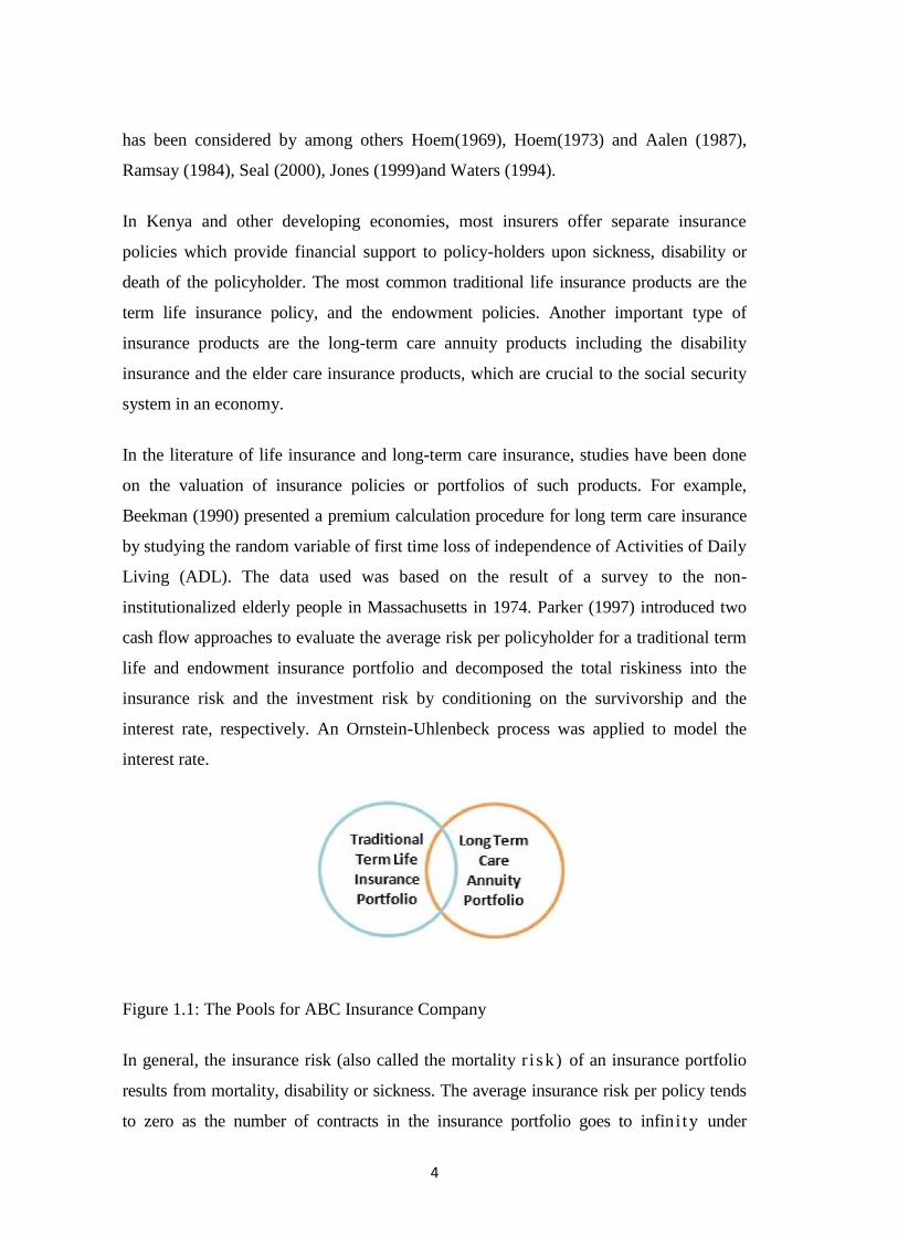
Figure 1.1: The Pools for ABC Insurance Company
In general, the insurance risk (also called the mortality r i sk) of an insurance portfolio
results from mortality, disability or sickness. The average insurance risk per policy tends
to zero as the number of contracts in the insurance portfolio goes to infini ty under
5
independent mortality assumption. Therefore, the insurance risk can be managed by risk
pooling within the insurance company. The insurance risk for an insurance portfolio
with a large size is relatively small compared to the investment risk which comes from
the fluctuations and the correlations of the periodic interest rates according to Parker
(1997). Marceau and Gaillardetz (1999) presented the reserve calculation for a life
insurance portfolio under stochastic mortalities and AR(1) interest rate assumptions.
However, it is not accurate to evaluate the insurance risk of the insurance company by
separately evaluating the risk of each insurance portfolio consisting of only one type of
insurance product. There might be some policyholders who are insured simultaneously by
different types of insurance products (Figure 1.1) . Therefore, independent mortality
assumption does not hold in these cases.
In considering an insurance portfolio one key issue that needs to be addressed for valuation
purposes is the methodology for calculating the transition probabilities including the
assumptions of the forces of transition. This has a huge impact on the valuation results.
A few papers discussing the health insurance cases have been published since 1980s.
Waters (1984) gave the basic concepts of the transition probabilities, the forces of
transition and their relationships. Ramsay (1984) studied the ruin probability of the
surplus of a sickness insurance contract which pays the benefit only if the duration of
the sickness exceeds certain period. Waters (1990) illustrated a method of calculating
the moment of benefit payments for a sickness insurance contract by introducing the
semi-Markov chain to model the transition process. In Jones (1994), a Markov chain
model was presented to calculate the transition matrix of a multi-state insurance
contracts consisting of three states with one-direction transitions only (e.g. healthy,
permanently disabled and deceased). Constant and piecewise forces of transition were
assumed in the paper. Levikson and Mizrahi (1994) priced a long term care contract with
three different care levels assuming that the policyholders health status could only either
remain unchanged or deteriorated.
1.3 Statement of the Problem
The Long Term Care (LTC) system in Kenya and other developing economies is largely
unfunded and characterized by an absence of risk pooling or a sophisticated user pays

6
mechanism. The system, therefore, stands somewhat isolated from many of its
counterparts overseas which combine private funding mechanisms such as private LTC
insurance with their respective State and publicly funded welfare programs. With the
exception of a limited number of accident compensation policies where LTC is insured
if attributable to accidents. Kenyan insurers do not currently engage in any form of LTC
insurance business. As such, the task of pricing and reserving for private LTC insurance
contracts for introduction into the Kenyan market is made difficult due to a lack of
historical experience, adequate data and consensus on appropriate modeling
methodology and assumptions.
The primary objective of this project, therefore, is to develop and test a multiple state
model for pricing and reserving LTC insurance using currently available Kenyan data.
In Leung (2004), a discrete time multiple state model was developed for projecting the
needs and costs of LTC in Australia. In this project, I relax the assumption of discrete
time and model the underlying process in a continuous time Markov framework. The
purpose of this project is to enable calculation of transition intensities for application in
Thiele's differential equation for pricing and reserving. This project concentrates on a
generalization of Thiele’s differential equation of multi-state markov model in
designing different types of long term care (LTC) insurances including a whole life
stand-alone LTC policy and LTC rider policy cover. The modeling framework and
results presented in this project may be used as a starting point for the development of
LTC insurance policies in Kenya.
1.4 Research Objectives
In this project, the general objective is to use the multistate markov framework to model
LTC insurance products in the Kenyan insurance industry.
In particular, the project intends to achieve the following specific objectives:
1. Estimate the transition probabilities of the t-year probability ab
xt p of a life aged
(x) making a transition from state a to state b of a four state Markov model using
Chapman-Kolmogorov and Forward Kolmogorov differential equations.

7
2. Calculate and graduate the maximum likelihood markov transition intensities or
forces of transition using the Compertz-Mekahem methods of graduation
3. Calculate benefit premiums for a set of illustrative hypothetical LTC insurance
products including a whole life stand-alone LTC policy and a LTC rider cover
using the equivalence principle/equation of value
4. Calculate the reserves of an illustrative hypothetical LTC whole life stand-alone
policy using Thiele’s differential equations
1.5 Justification of the Study
Current premium rates for the various LTC products varies from one insurer to another.
This is due to a lack of standard premium rate and its corresponding incident rate for the
various products sold. Some insurers charge higher premiums which results in the low
uptake rates of the product whereas others charge relatively low premium which also
results in the company running at a loss. This calls for the need to find a rigorous and
accurate formula for costing an LTC benefit product. This has necessitated the
determination of an accurate pricing formula. Pricing LTC products is a key objective
of any insurance industry that sells such a product. The project which considers the
various premiums and incidence rates for different age groups will serve as a platform
for insurers to know which group of people are most likely to suffer one condition than
the other. The idea of knowing that one must insure against conditions of not being able
to carry out one's normal duties, by virtue of suffering a major illness makes the project
very justifiable.
1.6 Significance of the Study
It is very significant for an insurance company to value or price its products correctly
such that such premium calculation is as accurate as possible. This indeed is true
especially for Long Term Care products whose impact on the insured and the
underwriter lasts for a long duration. Pricing of premium for the purchase of any
insurance forms the basics of any quality insurance in any insurance company. Thus the
data from the survey would therefore be of immense importance to the various
insurance companies in the country. These include the National Hospital Insurance

8
Fund from which the current data is obtained, Britam, Panafric Life, Lion, Pacis, C.I.C.,
Old Mutual, among others. The correct pricing and reserving of LTC products will
increase their sales and thereby increase the premium income of insurers. The
regulatory bodies such as Insurance Regulatory Authority(I.R.A.) and professional
insurance associations such as The Actuarial Society of Kenya(T.AS.K.), and
Association of Kenyan Insurers(A.K.I.) will benefit immensely from an accurate
valuation of LTC products in Kenya. At the end of the project, the various insurance
companies will have a better and scientific means of pricing and reserving the LTC
products.
9
2.0 CHAPTER TWO: LITERATURE REVIEW
2.1 Introduction
In this chapter the focus will be on the markov models in continuous time and discrete
state space two state, three and four state markov models. The chapter will begin with
the derivation and solution of the Kolmogorov forward and the Kolmogorov backward
equations by using the Chapman-Kolmogorov equations. Then focus will shift to
various versions of two, three and four state models with emphasis of the derivation and
solution of transition intensities/forces, , from one state to another, say, from
healthy to outpatient sickness using the Chapman-Kolmogorov equations and
Kolmogorov forward equations.
The three state process is commonly used to describe the state of an individual insured
under a disability income policy. In this case, premiums are payable while the insured is
in state 1, and benefits are payable while the insured is in state 2 (usually after a waiting
period). We will derive the probabilities of transition from one state to another via the
forces of intensities.
In this project, the four state multi state models from alive/healthy through out-patient
sickness, in-patient sickness all the way to death with recovery from either of the two
cases of sickness will be used to model the medical data from N.H.I.F. in order to
calculate premiums and reserves. The focus will be on deriving the probabilities of
transition from one state to another via the forces of intensities.
2.2 Chapman-Kolmogorov Equations
A Markov chain TttX
is called homogeneous, if it is time homogenous i.e. the following
equation holds for all s,t S such that 0][0 iXPandiXP ts (Scott W.F., 1999)
iXjXPiXjXP thtShs [][ (2.1)
For homogeneous Markov chain we use the notation :
hssPhP
hssphp ijij
,(:)(
),(:)(
(2.2)
10
Remarks that can be made are that a homogeneous Markov chain is characterized by the fact
that the transition probabilities and therefore also the transition matrices, only depend on the
size of the time increment and that for homogeneous Markov chain one can simplify the
Chapman – Kolmogorov equations to the semi group property.
)()()( tPsPtsP (2.3)
The semi – group property is popular in many different areas e.g. in quantum mechanics. The
mapping. )(),(: tPtRMTP n
Defines a one parameter semi – group.
2.3 Kolmogorov Forward and Backward Differential Equations
In the following section, we will only consider Markov chains on a finite state space (Lecture
notes, UoN, 2012). Thus point wise convergence and uniform convergence. Will coincide on S.
This enables us to give some of the proofs in a simpler form.
Definition: Let TttX
be a Markov chain with finite state space S and T SNforR we
define.
Nk
jkjN tsptsp ),().(
(2.4)
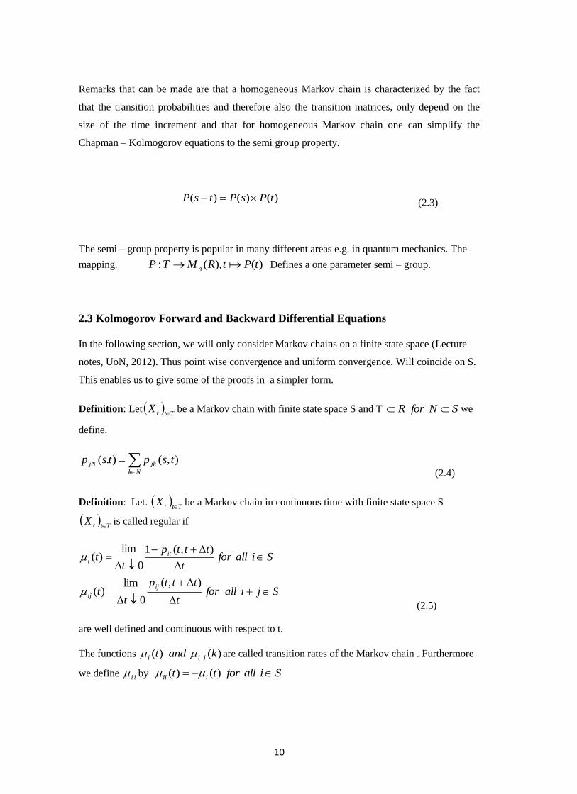
Definition: Let. TttX
be a Markov chain in continuous time with finite state space S
TttX
is called regular if
Sjiallfort
tttp
tt
Siallfort
tttp
tt
ij
ij
it
i
),(
0
lim)(
),(1
0
lim)(
(2.5)
are well defined and continuous with respect to t.
The functions )()( kandt jii are called transition rates of the Markov chain . Furthermore
we define ii by Siallfortt iii )()(
11
Remark that can be made is that the insurance model and the regularity of the Markov chain is
used to derive the differential equations which are satisfied by the mathematical reserve
corresponding to the policy.
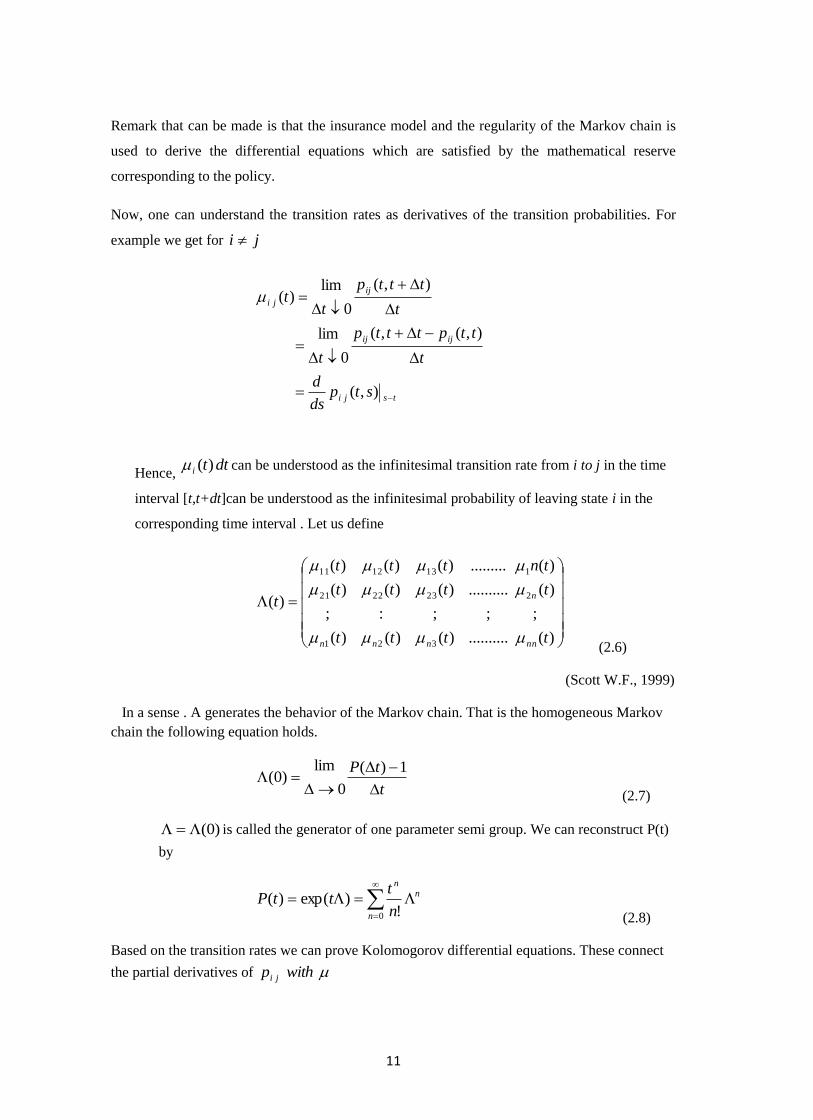
Now, one can understand the transition rates as derivatives of the transition probabilities. For
example we get for ji
tsji
ijij
ij
ji
stpds
d
t
ttptttp
t
t
tttp
tt
),(
),(,(
0
lim
),(
0
lim)(
Hence, dtti )( can be understood as the infinitesimal transition rate from i to j in the time
interval [t,t+dt]can be understood as the infinitesimal probability of leaving state i in the
corresponding time interval . Let us define
)(
;
)(
)(
..........)()()(
;;:;
..........)()()(
.........)()()(
)(2
1
321
232221
131211
t
t
tn
ttt
ttt
ttt
t
nn
n
nnn
(2.6)
(Scott W.F., 1999)
In a sense . A generates the behavior of the Markov chain. That is the homogeneous Markov
chain the following equation holds.
t
tP
1)(
0
lim)0(
(2.7)
)0( is called the generator of one parameter semi group. We can reconstruct P(t)
by
0 !
)exp()(n
nn
n
tttP
(2.8)
Based on the transition rates we can prove Kolomogorov differential equations. These connect
the partial derivatives of withp ji

12
Theorem (Kolmogorov):
Let TttX
be a regular Markov chain on a finite state space S. Then the following statements
hold. : (Backward differential equations)
),()(),(
),()(),()(),( 1,
tsPstsPds
d
tspstspstspds
d
ik
kjikjiji
The Kolmogorov Forward differential equations are
)(),(),(
)(),()(),(),(
ttsPtsPds
d
ttspttsptspdt
d
jk
kjkijijji
Proof:
The major part of the proof is based on the equations of Chapman and Kolmogorov.
We will prove the matrix version of the statement. This will help to highlight the key properties.
Let sssetands :0
`
0),()(
),(),(1(1
(
),(),(),((1),(),(
sfortsPs
tPsPs
tPsPtPss
tsPtp
Where we used the Chapman – Kolmogorov equation and the continuity of the matrix
multiplication.
Analogous one can prove the forward differential equation. Let 0.t
0)(),(
)1),((1
),(
),(),(),((1),(),(
tforttsP
tttPt
tsP
tsPtttPtsPtt
tsPttsP
13
An important remark is that the primary application of Kolmogorov’s difficult equations is to
calculate the transition probabilities jip based on the rates .
Now the definition that we let TttX
be a regular Markov chain on a finite state space S. We
denote the conditional probability to stay during the interval [s,t] in j by
ts
sjj jXjXPtsp,
),(
where s, t R , s t and Sj
In setting of a life insurance, this probability can for example be used to calculate the
probability that the insured survives 5 years. The following theorem illustrates how this
probability can be calculated based on the transition rates.
Theorem: Let TttX
be a regular Markov chain
(Scott W.F., 1999).
jk
t
jkjj dtsp8
)(exp),(
Holds for 0][, jXPifts s
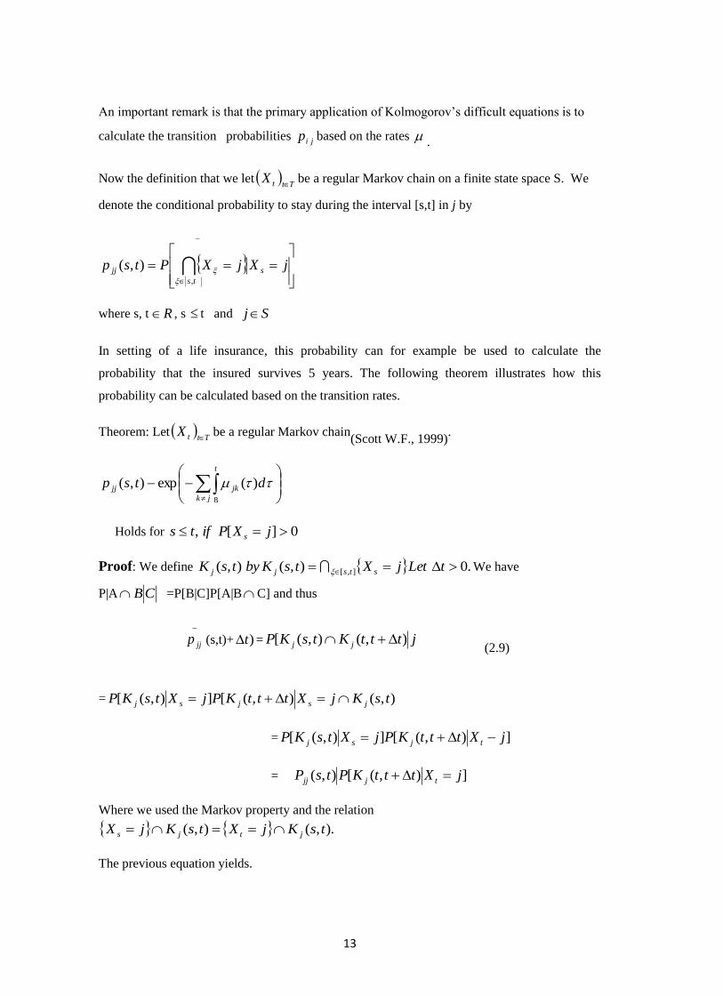
Proof: We define .0),(),( ],[ tLetjXtsKbytsK stsjj We have
P|A CB =P[B|C]P[A|BC] and thus
jjp (s,t)+ )t = jtttKtsKP jj ),(),([ (2.9)
= ),(),([]),([ tsKjXtttKPjXtsKP jsjsj
= ]),([]),([ jXtttKPjXtsKP tjsj
= ]),([),( jXtttKPtsP tjjj
Where we used the Markov property and the relation
).,(),( tsKjXtsKjX jtjs
The previous equation yields.
14
)(),(),(
]),([1(),(),(),(
totttptsp
jXtttKPtsptspttsP
jk
kjjj
tjjjjjjj
(2.10)
where we used that the rates are well defined. Now taking the limit we get the differential
equation
jk
jkjjjj ttsptspdt
d)(),(),(
(2.11)
Solving this equation with the boundary condition
1),( ssp jj yields the statement of the
theorem.
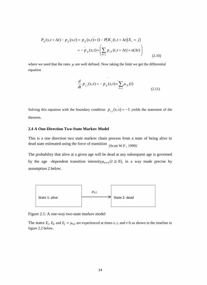
2.4 A One-Direction Two-State Markov Model
This is a one direction two state markov chain process from a state of being alive to
dead state estimated using the force of transition (Scott W.F., 1999)
.
The probability that alive at a given age will be dead at any subsequent age is governed
by the age –dependent transition intensity , in a way made precise by
assumption 2 below.
Figure 2.1: A one-way two-state markov model
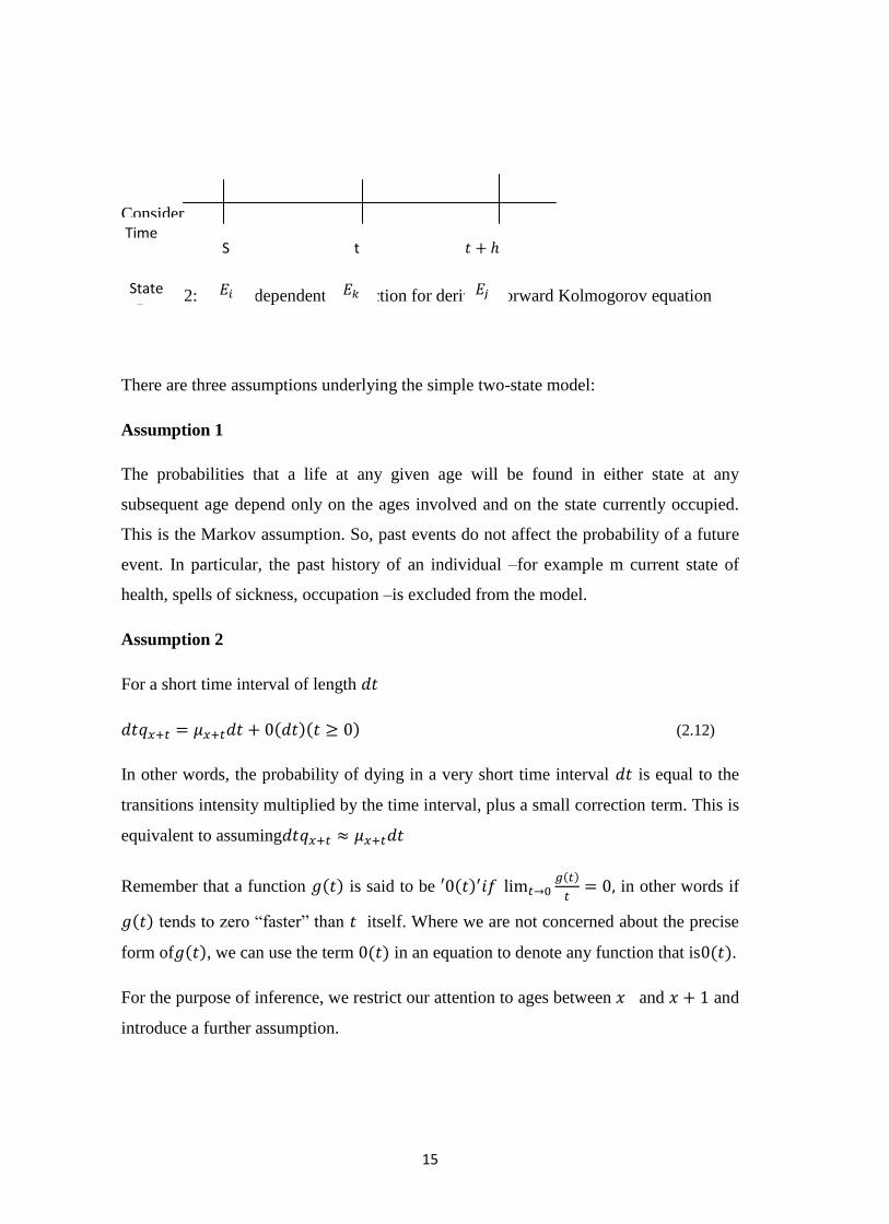
The states , and are experienced at times s, t, and t+h as shown in the timeline in
figure 2.2 below.
State 1: alive
State 2: dead
15
Consider
Figure 2.2: A time dependent transaction for deriving forward Kolmogorov equation
There are three assumptions underlying the simple two-state model:
Assumption 1
The probabilities that a life at any given age will be found in either state at any
subsequent age depend only on the ages involved and on the state currently occupied.
This is the Markov assumption. So, past events do not affect the probability of a future
event. In particular, the past history of an individual –for example m current state of
health, spells of sickness, occupation –is excluded from the model.
Assumption 2
For a short time interval of length
(2.12)
In other words, the probability of dying in a very short time interval is equal to the
transitions intensity multiplied by the time interval, plus a small correction term. This is
equivalent to assuming
Remember that a function is said to be
in other words if
tends to zero “faster” than itself. Where we are not concerned about the precise
form of , we can use the term in an equation to denote any function that is .
For the purpose of inference, we restrict our attention to ages between and and
introduce a further assumption.
Time S t
State
16
Assumption 3
Our investigation will consist of many observations of small segments of lifetimes i.e.
single years of age. Assumption 3 simplifies the model by treating the transition
intensity a constant for all individuals aged last birthday. This does not mean that we
believe that the transition intensity will increase by a discrete step when an individual
reaches age , although this is a consequence of the assumption.
Now by the Chapman –Kolmogorov equation:
For the two state one direction markov model
(2.13)
Thus Kolmogorov forward differential equations are:
17
(2.14)
In the matrix form we have:
Therefore
(2.15)
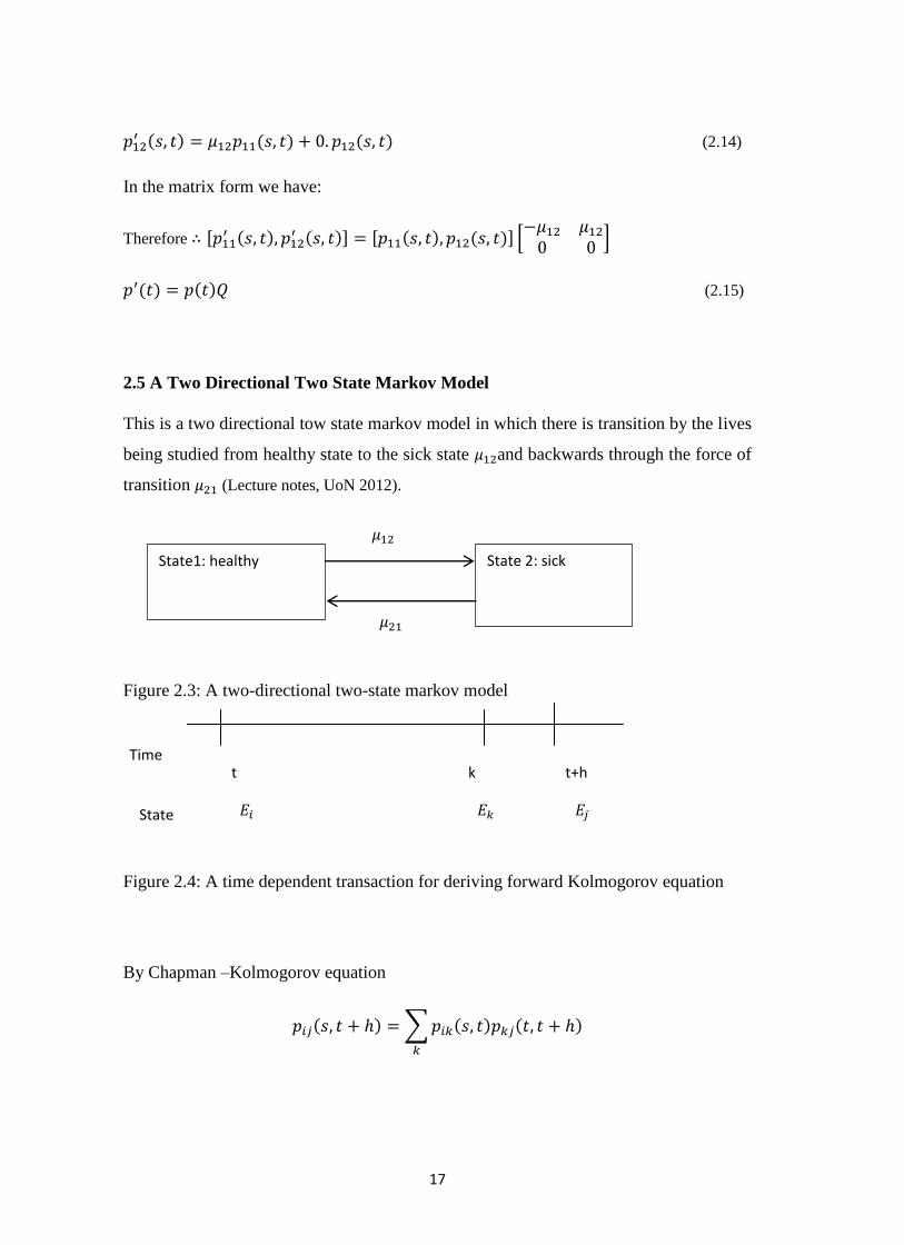
2.5 A Two Directional Two State Markov Model
This is a two directional tow state markov model in which there is transition by the lives
being studied from healthy state to the sick state and backwards through the force of
transition (Lecture notes, UoN 2012).
Figure 2.3: A two-directional two-state markov model
Figure 2.4: A time dependent transaction for deriving forward Kolmogorov equation
By Chapman –Kolmogorov equation
State1: healthy State 2: sick
t Time
State
k
t+h
18
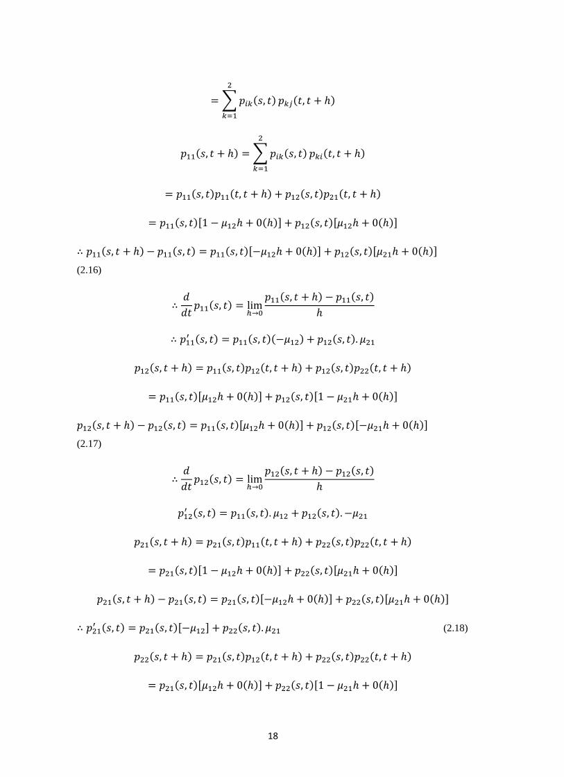
(2.16)
(2.17)
(2.18)
19
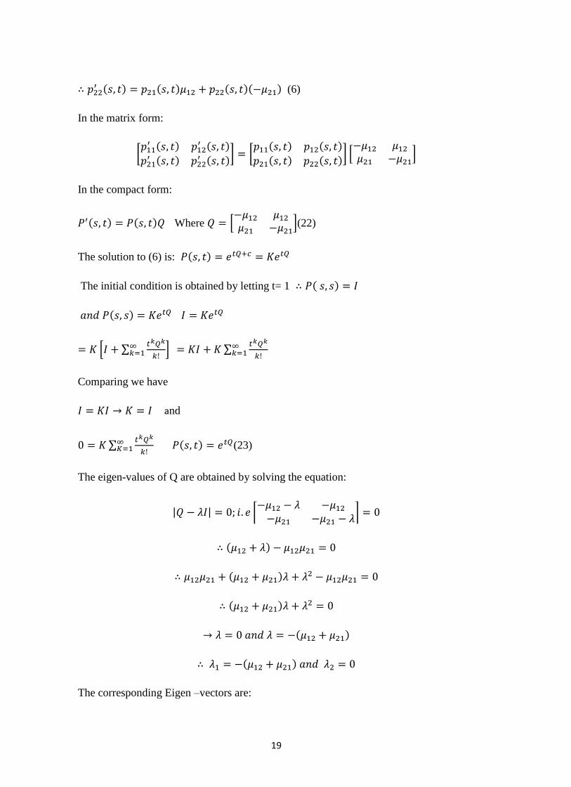
(6)
In the matrix form:
In the compact form:
Where
(22)
The solution to (6) is:
The initial condition is obtained by letting t= 1
Comparing we have
and
(23)
The eigen-values of Q are obtained by solving the equation:
The corresponding Eigen –vectors are:
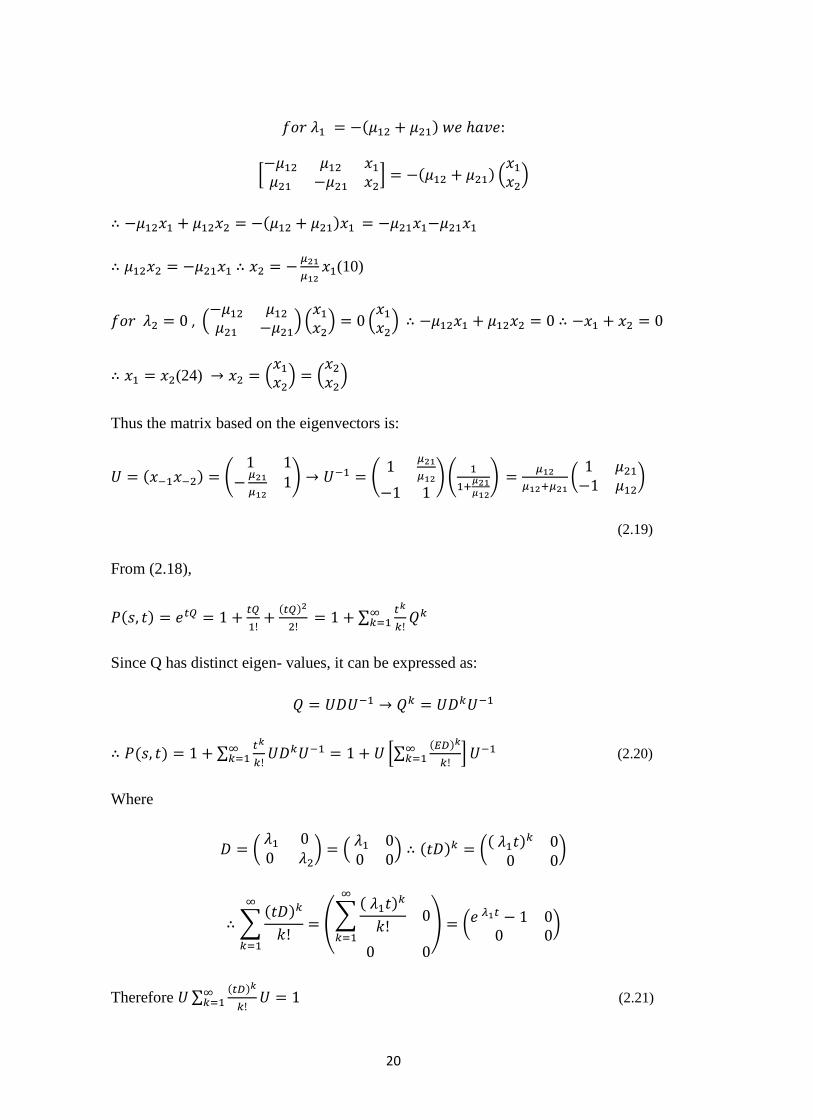
20
(10)
,
(24)
Thus the matrix based on the eigenvectors is:
(2.19)
From (2.18),
Since Q has distinct eigen- values, it can be expressed as:
(2.20)
Where
Therefore
(2.21)
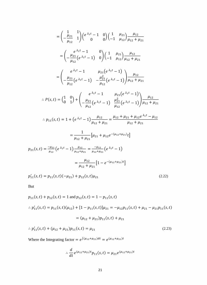
21
(2.22)
But
and
(2.23)
Where the Integrating factor
22
When t =j then we have:
(2.24)
From (2.18)
23
(2.25)
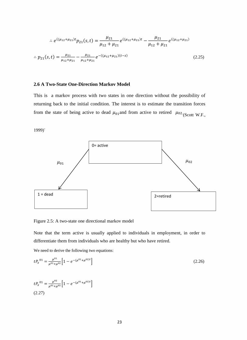
2.6 A Two-State One-Direction Markov Model
This is a markov process with two states in one direction without the possibility of
returning back to the initial condition. The interest is to estimate the transition forces
from the state of being active to dead and from active to retired (Scott W.F.,
1999).
Figure 2.5: A two-state one directional markov model
Note that the term active is usually applied to individuals in employment, in order to
differentiate them from individuals who are healthy but who have retired.
We need to derive the following two equations:
(2.26)
(2.27)
0= active
1 = dead 2=retired
µ02
24
Again by the Chapman-Kolmogorov equation
But and
and
Replacing 1 by 2 and vice versa we have:
as required to show. (2.28)
25
The term in brackets is the probability of having left the active state and the fraction
gives the conditional probability of each decrement having occurred , given that have
of them has occurred.
where (2.29)
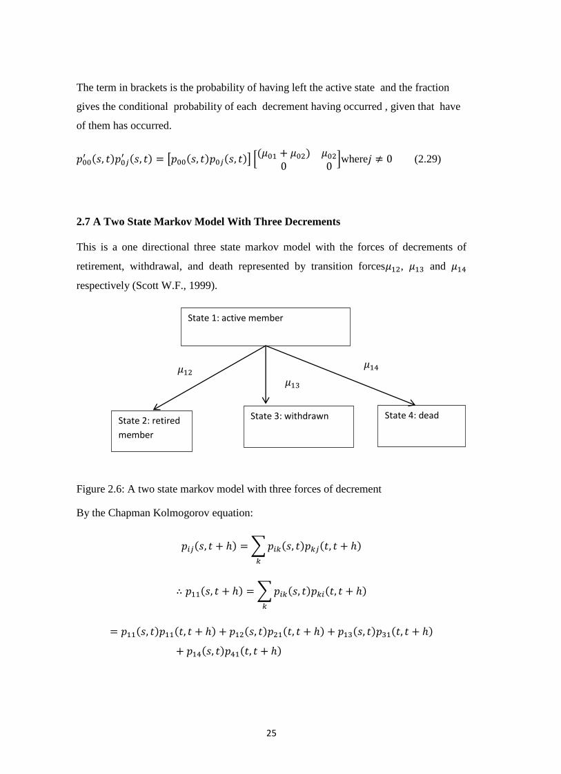
2.7 A Two State Markov Model With Three Decrements
This is a one directional three state markov model with the forces of decrements of
retirement, withdrawal, and death represented by transition forces , and
respectively (Scott W.F., 1999).
Figure 2.6: A two state markov model with three forces of decrement
By the Chapman Kolmogorov equation:
State 1: active member
State 2: retired
member
State 3: withdrawn State 4: dead
26
and
and
(2.30)
Next we have
Hence
and
(2.31)
In general
and
27
(2.32)
and
(2.33)
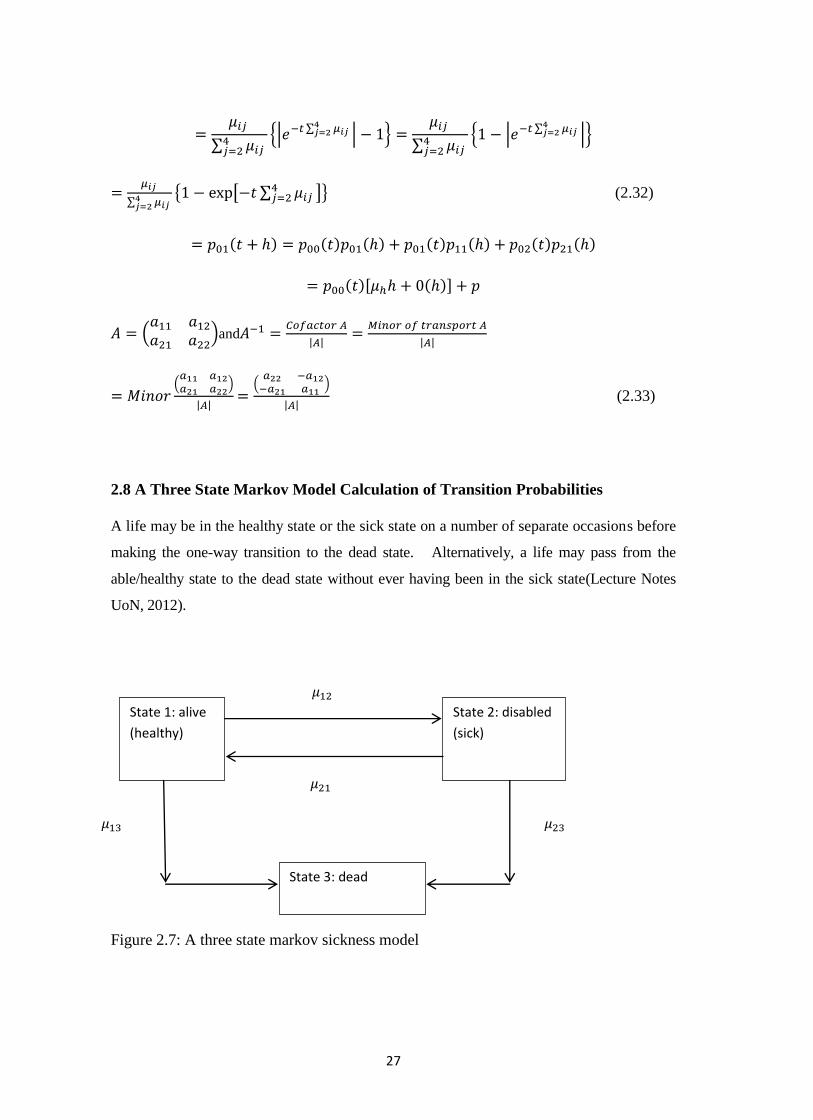
2.8 A Three State Markov Model Calculation of Transition Probabilities
A life may be in the healthy state or the sick state on a number of separate occasions before
making the one-way transition to the dead state. Alternatively, a life may pass from the
able/healthy state to the dead state without ever having been in the sick state(Lecture Notes
UoN, 2012).
Figure 2.7: A three state markov sickness model
State 1: alive
(healthy)
State 2: disabled
(sick)
State 3: dead
28
Now, by the Chapman-Kolmogorov equation
(2.34)
Where
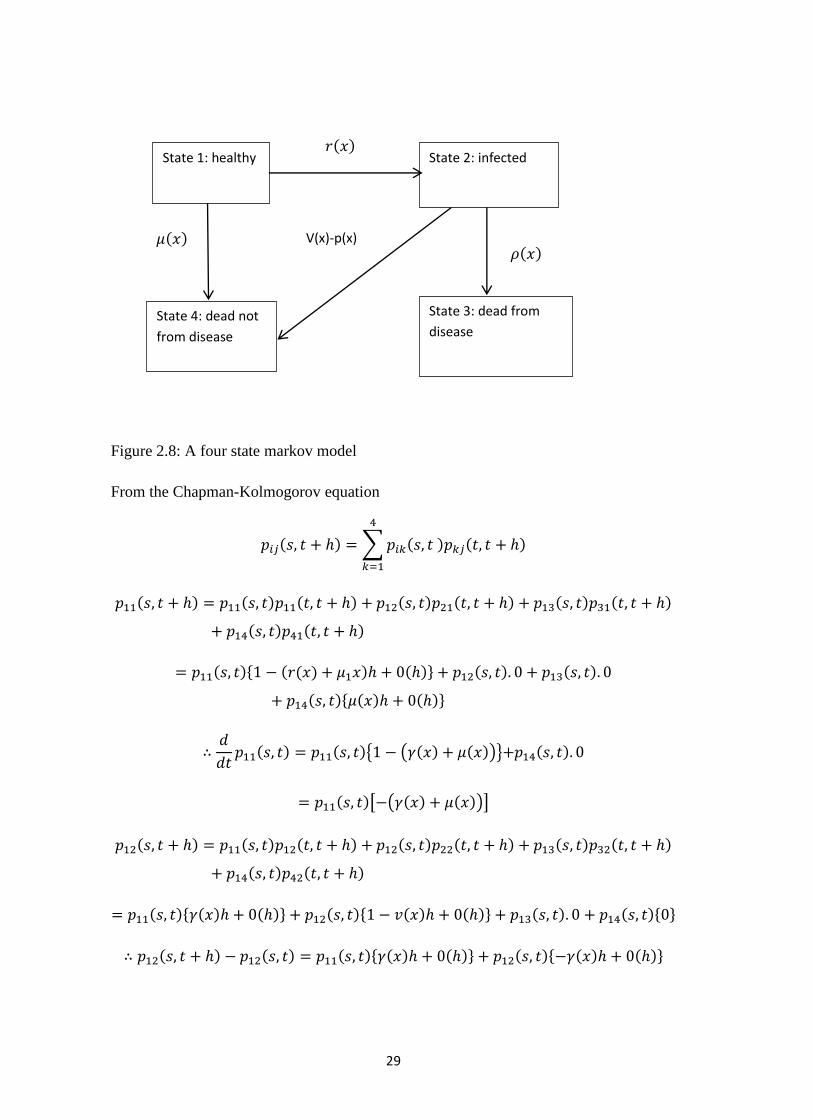
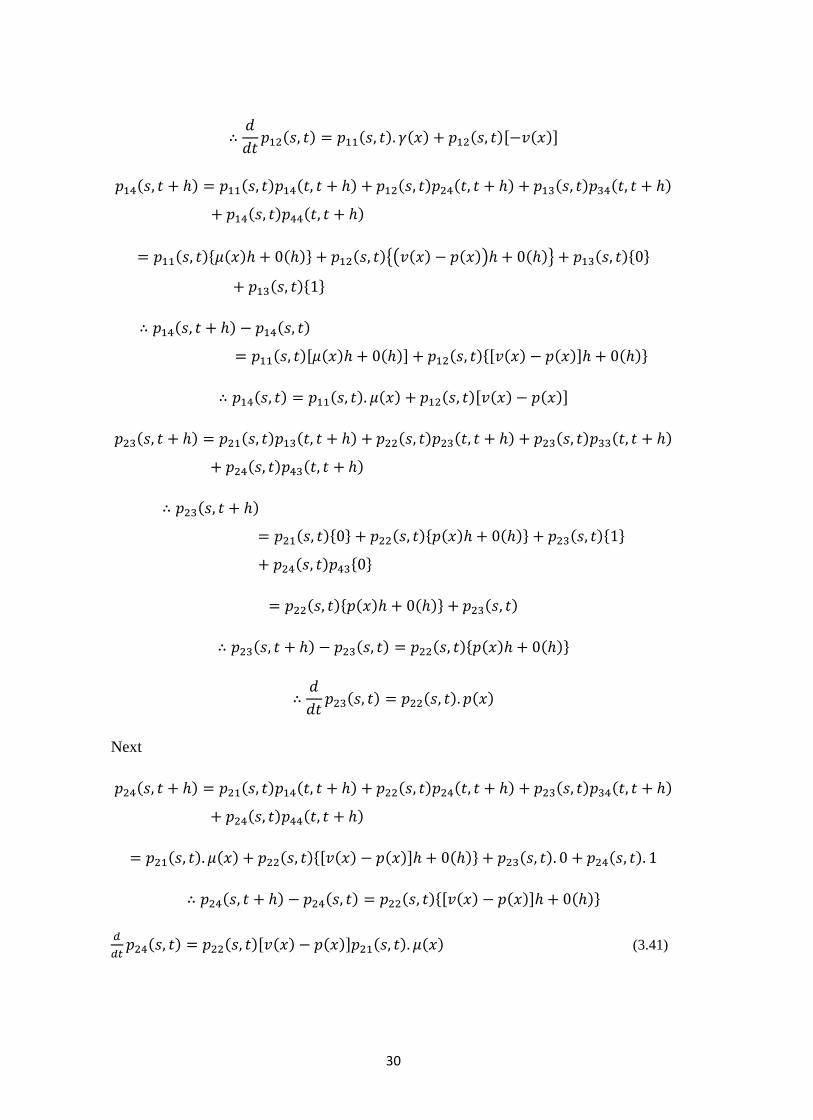
2.9 A Four State Markov Model – Version I
In the second type of the four state markov process, a life move from healthy to a sick
and infected state. Then death can occur as a result of the infection or death could also
occur from causes not related with the disease infection(Lecture Notes UoN, 2012).
29
Figure 2.8: A four state markov model
From the Chapman-Kolmogorov equation
State 1: healthy State 2: infected
State 4: dead not
from disease
State 3: dead from
disease
V(x)-p(x)
30
Next
(3.41)

31
(3.42)
All these models from the two state to the four state model version I are reviewed as a
prelude to the four state model discussed in the methodology chapter three with healthy,
out patient, in patient and death states which is the actual model that was applied in his
study to the medical data obtained from e N.H.F. in Kenya.
2.11 Empirical Review
The use of Markov chains in life contingencies and their extension has been proposed
by several authors, in both the time-continuous case and the time-discrete case; for
example, see Amsler (1968), Amsler (1988), Haberman (1983), Haberman (1984),
Hoem (1969), Hoem (1988), Jones (1993), Jones (1994), Wilkie (1988). The earliest
paper, by Walker (1990), provides a brief introduction to the issues surrounding LTC
insurance pricing and provides specimen net single and annual renewable premiums for
a LTC benefit using illustrative morbidity rates for males, females and couples. Walsh
and de Ravin (1995) perform similar calculations based on data sourced from the 1993
ABS survey of Disability, Ageing and Carers and calculated premium rates directly
from prevalence rate data. The mathematical methodologies are not detailed in their
respective papers, but it is clear that in both papers, calculations are based on an
inception-annuity approach framework.
32
There has been a great deal of research which makes use of Multiple State models to
provide a powerful tool for application in many areas of Actuarial Science, particularly
in the Actuarial Assessment of sickness insurance and disability income benefits.
The early history of these models has been described by Seal (1977) and Daw (1979) in
some detail and our purpose here is merely to outline the key historical developments in
terms of the theory and its practical applications to insurance problems. The problem is
the following:
Given two states A and B such that individuals in state A have mutually exclusive
probabilities, possibly dependent on the time spent in state A, and the possibility of
leaving state A because if (i) death or (ii) passage to state B, then what is the probability
of an individual passing to state B and dying there within a given period?
Bernoullis state A consisted of individuals who had never had smallpox, while state B
comprised those who had contracted smallpox and would either die from it, almost
immediately, or survive and no longer be suffering from that disease. In solving this
problem, Bernoulli started with Edmund Halleys (Breslau) life table and effectively
produced the first double decrement life table with one of the related single decrement
tables as well as considering the efficacy of inoculation and deriving a mathematical
model of the behaviour of smallpox. During the next 50 years, there were a number of
contributions from other authors on the subject, including Jean dAlembert and Jean
Trembley.
Lambert (1772) explained how numerical data could be used to study Bernoullis
problem and laid the practical foundations for the double decrement model and life
table. He obtained an approximate formula for the rate of mortality and thereby setting
down a practical connection between the double decrement model and the underlying
single decrement models. Despite this progress by the early 1 800s there were two
outstanding problems, namely (i) deriving accurate practical formulae for application to
numerical data, linking the discrete and continuous cases; and (ii) obtaining exact
results in a convenient form (d¶Alembert had derived an exact results in terms of an
33
integral that was difficult to evaluate). These problems were attacked successfuly and
independently by Cournot (1843) and Makeham (1867). They were the first to set down
the fundamental relations of multiple decrement models: in modern notation:
for k = 1, 2,…, m
(3.43)
Makeham (1867) also contains an analysis of the „partial forces of mortality for
different causes of death, suggesting an interpretation of his well –known formula for
the aggregate force of mortality to represent separate contributions from m + n causes of
death. Makeham went on to use connection between forces of decrement to interpret the
prior development of the theory; he demonstrated that the earlier results of Bernoulli
and d¶Alembert satisfied this addictive law for the forces of decrement and this
multiplicative law for the probabilities (or corresponding functions).
In an internal report in 1875 (which was not placed in the public domain) on the
invalidity and widows pension scheme for railway officials, Karup described the
properties and use of singe decrement probabilities and forces of decrement in the
context of an illness-death model (with no recoveries permitted), i.e. the „independent
or pure¶ probabilities of mortality and disablement. Hamza (1900) represents an
important development by providing a systematic approach to disability benefits in both
the continuous and discrete cases. Hamza’s paper is significant, setting down a notation
which has been widely adopted in the following decades and which forms the basis for
the notation we have utilized.
Pasquier took a dramatic step forward by providing a rigorous, mathematical discussion
of the invalidity or sickness process with the introduction of a three state-death model in
which recoveries were permitted. He derived the full differential equations for the
transition probabilities and showed that these lead to a second-order differential of
Riccati type which he then solved for the case of constant forces of transition. Du
Pasquier work is very significant, presenting an early application of Markov Chains,
and laying the foundations for modern actuarial applications to disability insurance,
long-term care insurance and critical illness.
34
Despite the interest and importance of these problems to actuaries and the consistent
contribution made to the actuarial literature since the mid-nineteenth century, these
contributions have essentially been rediscovered and renamed as the Theory of
competing risk by Neyman (1950) and Fix and Neyman (1951), and other statistical
workers.
Applications of semi-Markov models to actuarial (and demographic) problems was
done by Hoem (1972); the first application of semi-Markov processes to disability
benefits appears in Janssen (1966). As far as disability benefits are concerned, the
mathematics of Markov and semi-Markov chains provides both a powerful modelling
tool and a unifying point of view, from which several calculation techniques and
conventional procedures can be seen in a new light (seeHaberman (1988), Waters (1984),
Waters (1989), Continuous Mortality Investigation Bureau (1991), Pitacco (1995)).
2.12 Critical Review
A range of methodologies have been applied to pricing LTC insurance including
inception annuity approaches (Gatenby 1991) or risk renewal approaches (see Beekman
1989). Though an explicit and systematic use of the mathematics of multiple state
(Markov and semi-Markov) models dates back to the end of the 1960s, it must be
stressed that the basic mathematics of what we now call a Markov chain model were
developed during the eighteenth century (see Seal (1977)); seminal contributions by D.
Bernoulli and P.S. de Laplace demonstrate this for the time-continuous case. Moreover,
the well known paper of Hamza (1900) provides the actuarial literature with the first
systematic approach for disability benefits, in both the continuous and discrete case.
Keyfitz and Rogers provide a method for determining transition probabilities under a
Markov process. The approach was developed by assuming that forces of transition are
constant within age intervals of a fixed length. Transition probability matrices were then
calculated re-cursively for time periods that are multiples of this age interval.
Multiple state models are prevalent in the actuarial literature in areas including Life
Insurance (see Pitacco 1995), Permanent Health Insurance (PHI) in the UK (see Waters
1984, Sansom and Waters 1988, Haberman 1993, Renshaw and Haberman 1998,

35
Cordeiro (2001) and Disability Income Insurance (see Haberman and Pitacco 1999). It
is therefore unsurprising that the suitability of multiple state modeling for LTC
insurance has been well recognized and consequently applied. For instance, Levikson
and Mizrahi (1994) consider an `upper triangular' (UT) multiple state model in the
general Markovian framework where three care levels are considered and the insured
life proceeds through the deteriorating stages of ADL failure until death. Premium
calculation is subsequently performed via a representation of the discounted value of
future benefits in a particular care level as a random variable. Similar frameworks have
been studied by Alegre et al (2002), who also consider a LTC system with no recoveries
and premium calculations derived by calculating annuity values in discrete time for a
life in a LTC claiming state. Moreover, the valuation of LTC annuities to price LTC
insurance in continuous time has been discussed by Pitacco (1993) and Czado and
Rudolph (2002).
The chosen methodology in this project is a multiple state modeling approach within a
continuous time Markov framework with premiums and reserves calculated by means of
applying generalizations of Thiele's differential equations. This choice is motivated by
the benefits of multiple state modeling being an accurate representation of the
underlying insurance process, a greater degree of flexibility and scope for scenario
testing and the ease of monitoring actual experience against expected at a practical level
(Gatenby and Ward 1994, Robinson 1996 and Society of Actuaries Long-Term Care
Insurance Valuation Methods Task Force 1995).
Despite the wide range of methodologies considered abroad, only limited literature
concerning pricing LTC insurance contracts in Kenya, especially the use of multi state
modeling within a markov framework and application of Chapman-Kolmogorov and
Thiele’s differential equations, has been published. This project therefore intends to fill
this research gap.
36
CHAPTER THREE: METHODOLOGY
3.1 Introduction
This chapter focuses on the estimation of probabilities of transition from one state to
another using the type II four state markov model which involves the healthy, out
patent sickness , in patient sickness and death. Then the parametric estimation of the
maximum likelihood estimates of the forces of transition
, , from one state to another,
the general case, then the properties of the maximum likelihood estimators, the
alternative derivation of the maximum likelihood estimates. The parametric graduation
methods of Compertz and Mekahem with their logarithmic modification including the
Perks formula with be outlined. The use of the equivalence principle in calculating
premiums for some hypothetical Long Term Care insurance products will be described.
Finally, the use Thiele’s differential equation in calculating reserves will be explained.
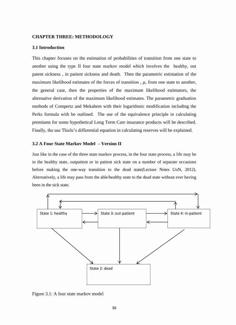
3.2 A Four State Markov Model – Version II
Just like in the case of the three state markov process, in the four state process, a life may be
in the healthy state, outpatient or in patient sick state on a number of separate occasions
before making the one-way transition to the dead state(Lecture Notes UoN, 2012).
Alternatively, a life may pass from the able/healthy state to the dead state without ever having
been in the sick state.
Figure 3.1: A four state markov model
State 1: healthy State 3: out-patient State 4: in-patient
State 2: dead
37
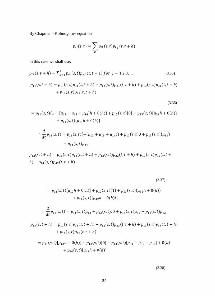
By Chapman –Kolmogorov equation
In this case we shall use:
(3.35)
(3.36)
(3.37)
(3.38)
38
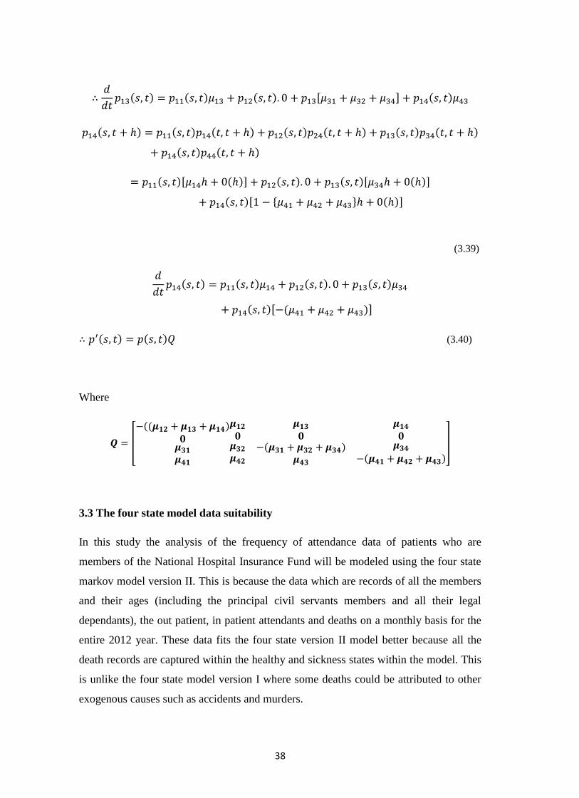
(3.39)
(3.40)
Where
3.3 The four state model data suitability
In this study the analysis of the frequency of attendance data of patients who are
members of the National Hospital Insurance Fund will be modeled using the four state
markov model version II. This is because the data which are records of all the members
and their ages (including the principal civil servants members and all their legal
dependants), the out patient, in patient attendants and deaths on a monthly basis for the
entire 2012 year. These data fits the four state version II model better because all the
death records are captured within the healthy and sickness states within the model. This
is unlike the four state model version I where some deaths could be attributed to other
exogenous causes such as accidents and murders.
39
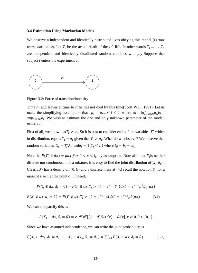
3.4 Estimation Using Markovian Models
We observe n independent and identically distributed lives obeying this model (Lecture
notes, UoN, 2012). Let be the actual death of the life. In other words
are independent and identically distributed random variables with Suppose that
subject enters the experiment at
Figure 3.2: Force of transition/intensity
Time and leaves at time if he has not died by this time(Scott W.F., 1991). Let us
make the simplifying assumption that where
We wish to estimate the one and only unknown parameter of the model,
namely .
First of all, we know that . So it is best to consider each of the variables which
in distribution, equals given that . What do we observe? We observe that
random variables and where
Note that , by assumption. Note also that is neither
discrete nor continuous; it is a mixture. It is easy to find the joint distribution of .
Clearly, has a density on and a discrete mass at .( recall the notation for a
mass of size 1 at the point c) . Indeed,
(3.1)
We can compactify this as
Since we have assumed independence, we can write the joint probability as
(3.2)
0 1
40
Here the variables take the values in respectively, while the
take values 0 or 1 each. Thus, the likelihood corresponding to the
observations is
The maximum likelihood estimation is defined by
And is easily found to be
/
(3.3)
Note that is a veritable statistic for it is just a function of the observations.
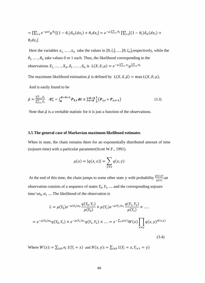
3.5 The general case of Markovian maximum likelihood estimates
When in state, the chain remains there for an exponentially distributed amount of time
(sojourn time) with a particular parameter(Scott W.F., 1991).
At the end of this time, the chain jumps to some other state with probability
an
observation consists of a sequence of states and the corresponding sojourn
time’s The likelihood of the observation is
(3.4)
Where and

41
Are the total sojourn time in state and the total number of jumps from state to
state , respectively, for the sequence of our observations
Two things may happen when we observe a Markov chain, either we stop observing at
some predetermined time or the Markov chain reaches an absorbing state and, a fortiori,
we must stop the observation . For instance, in the Markov chain figure 4.8, there are
three absorbing states: and two transient ones: 1, 2. if we start with we
may be
Figure 3.3: Three Absorbing States
Lucky and observe that 1,2,1,2,1,2,1,2,1,2,1,2……
For long time, at some point we will get bored and stop, or we may observe either of the
Following trajectories , , and
The likelihoods in each case are
The quantities take values 0 or 1 and amongst them, only one is
1. So we can summarize the likelihood in
b 2 1
a
c
42
(3.5)
This is an expression valid for all trajectories. Clearly, where as it may be possible to
estimate with the observation of one trajectory alone, this is not the case with the
remaining parameters; we need independent trials of the Marko chain. Thus, if we run
the Markov chain times, independently trials of to time, a moment of reflection shows
the form of likelihood remains the same as in the last display, provided we interpret
as the total sojourn time in state over all observations. Same interpretation
holds for the quantities .
Thus the general expressions are valid, in the same manner, for independent trials. To
do this, recall that and write the log likelihood as
So, for a fixed pair of distinct states
Setting this equal to zero obtains the MLE estimator
(3.6)
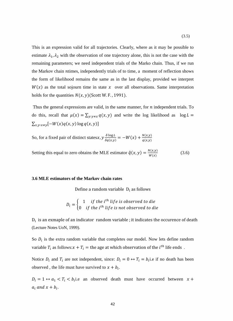
3.6 MLE estimators of the Markov chain rates
(Lecture Notes UoN, 1999).
So is the extra random variable that completes our model. Now lets define random
variable as follows: .
Notice and are not independent, since: i.e if no death has been
observed , the life must have survived to .
i.e an observed death must have occurred between
.
43
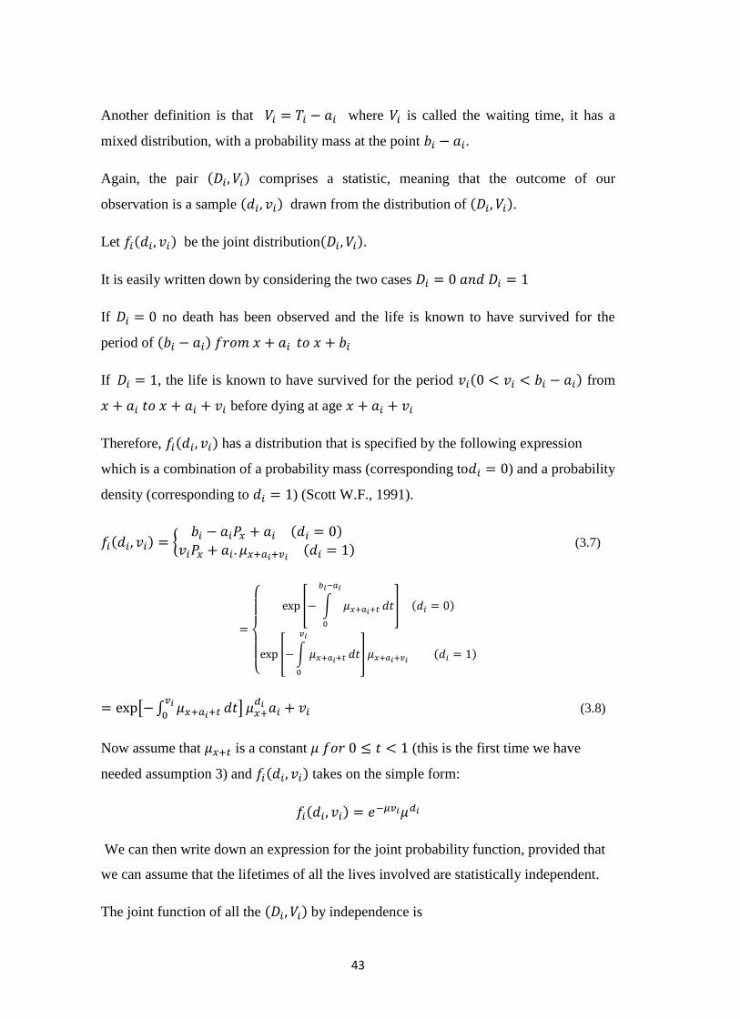
Another definition is that where is called the waiting time, it has a
mixed distribution, with a probability mass at the point .
Again, the pair comprises a statistic, meaning that the outcome of our
observation is a sample drawn from the distribution of .
Let be the joint distribution .
It is easily written down by considering the two cases
If no death has been observed and the life is known to have survived for the
period of
If , the life is known to have survived for the period from
before dying at age
Therefore, has a distribution that is specified by the following expression
which is a combination of a probability mass (corresponding to ) and a probability
density (corresponding to ) (Scott W.F., 1991).
(3.7)
(3.8)
Now assume that is a constant (this is the first time we have
needed assumption 3) and takes on the simple form:
We can then write down an expression for the joint probability function, provided that
we can assume that the lifetimes of all the lives involved are statistically independent.
The joint function of all the by independence is
44
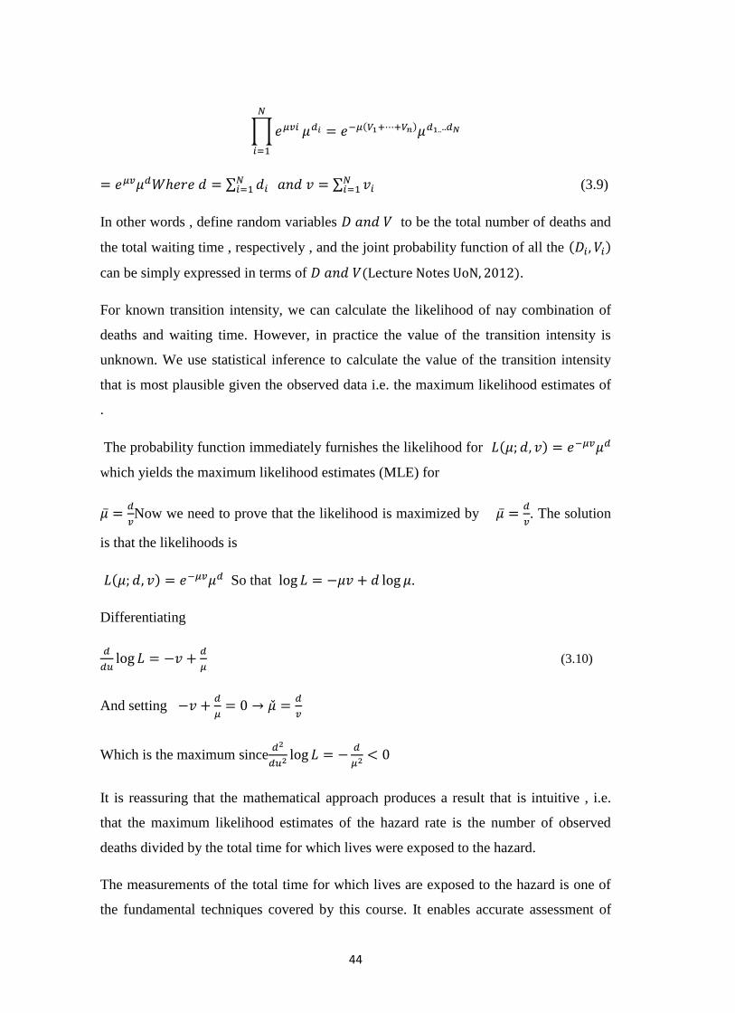
(3.9)
In other words , define random variables to be the total number of deaths and
the total waiting time , respectively , and the joint probability function of all the
can be simply expressed in terms of .
For known transition intensity, we can calculate the likelihood of nay combination of
deaths and waiting time. However, in practice the value of the transition intensity is
unknown. We use statistical inference to calculate the value of the transition intensity
that is most plausible given the observed data i.e. the maximum likelihood estimates of
.
The probability function immediately furnishes the likelihood for
which yields the maximum likelihood estimates (MLE) for
Now we need to prove that the likelihood is maximized by
. The solution
is that the likelihoods is
So that .
Differentiating
(3.10)
And setting
Which is the maximum since
It is reassuring that the mathematical approach produces a result that is intuitive , i.e.
that the maximum likelihood estimates of the hazard rate is the number of observed
deaths divided by the total time for which lives were exposed to the hazard.
The measurements of the total time for which lives are exposed to the hazard is one of
the fundamental techniques covered by this course. It enables accurate assessment of
45
risks, from the probability of a policyholder dying to the probability of a claim under a
motor insurance policy(Lecture Notes UoN, 2012).
3.7 Properties of The Maximum Likelihood Estimator
The estimate , being a function of the sample of the samples values d and v, can itself
be regarded as a sample value drawn from the distribution of the corresponding
estimator:
So, the estimator is a random variable and the maximum likelihood estimate is the
observed value of that random variable(Lecture Notes UoN, 2012).
It is important in application to be able to estimate the moments of the estimator , for
example to compare the experience with that of a standard table. At least, we need to
estimate .
In order to derive the properties of the estimator we will use two results that link the
random variables .
The following exact results are obtained
and (3.11)
Note that the first of these can also be written as
In the case that the are known constants, this follows from integrating
/summing the probability function of over all possible events to obtain:
And then differentiating with respect to , once to obtain the mean and twice to obtain
the variance
We will show how to use this to prove result (1) above in moment, but first we need to
derive two other results. (The derivation of result (2) is covered in the question &
answer bank).
46
We can how that
(3.12)
As a solution, since if the life is not observed to die, we only need to consider
the probability of death occurring
We are assuming constant transition intensity(Lecture Notes UoN, 2012).
Hence
In order to show that
The solution will be as follows:
Hence
(3.13)
Proof of (1)
Differentiating (*) with respect to gives;
(Because the limits of the integrals don’t depend on , this just involves differentiating
the expressions inside the integral with respect to
47
Multiplying throughout by then gives:
(3.14)
We can see that the first term is and the expression is curly brackets is
So As required (Lecture Notes UoN, 2012).
3.8 The Distribution of
To find the asymptotic distribution of consider:
(Lecture Notes UoN, 1999).
(3.15)
So, by the central limit theorem:
and
Then note that (not rigorously):
By the law of large numbers, (technically, this refers to “convergence in
probability “) and
(3.16)
But we know that
So, asymptotically:
(3.17)
3.9 Alternative Derivation of
In this section we describe another way of deriving the asymptotic distribution of , the
maximum likelihood estimator of .
48
We start from the likelihood function:
The log likelihood is then
and differentiating this with respect to gives:
setting this equal to 0 and solving for yields the required maximum
likelihood estimate:
We can check that this does maximize the likelihood, by examining the sign o the
second derivative of the log likelihood.
(3.18)
The corresponding maximum likelihood estimator is:
Where D and V are random variables denoting the number of deaths and the total
waiting time, respectively.
3.10 Exact Calculation of The Central Exposed to Risk
Central exposed to risk (or waiting times) are very natural quantities, intrinsically
observable even if observation may be incomplete in practice, that is, just record the
time spent under observation by each life. Note that this is so even if lives are
observed for only part of the year of age [x, x +1] whatever reason(Lecture Notes UoN,
2012).
(a)Working with complete data
The procedure for the exact calculation of is obvious: record all dates of birth,
record all dates of entry into observation, record all dates of exit from observation and
then compute. If we add to the data above the cause of the cessation of observation, we
have dx as well, and we have finished. The central exposed to risk for a life with age
label x is the time from Date A to Date B where: Date A is the latest of: the date of
49
reaching age label x of the start of the investigation and the date of entry. Date B is the
earliest of; the date of reaching age label x +1, the end of the investigation and the date
of exit (for whatever reason).
(b) Census approximation of from available data
We will consider how to calculate approximately when the exact dates of entry to
and exit from observation have not been recorded. Suppose that we have death data of
the form: Total number of deaths age x last birthday during calendar years
2(Scott W.F., 1991).
That is, we have observations over N+1 calendar years of all deaths between ages x and
x +1.
However, instead of the times of entry to and exit from observation of each fife being
known, we have instead only the following census data:
= Number of lives under observation aged x last birthday at time t where t 1
January in calendar years K, K + 1,..., K + N,K + N + 1
Now define P x , t to be the number of lives under observation, aged x last birthday, at
anytime t . Note that:
During any short time interval there will be , lives each contributing a
fraction of a year dt to the exposure. So, integrating over the observation
period gives the total central exposed to risk for this age. In other words. is the area
under the "curve" between .
The problem is that we do not know the value of for all . So we cannot work out the
exact value of the integral. We have the values of only if t is a 1 January
(a census date), so we must estimate from the given census data. The problem
reduces to estimating an integral, given the integrand at just a few points (in this case,
integer spaced calendar times). This is a routine problem in numerical analysis.
The simplest approximation, and the one most often used, is that is linear
between census dates, leading to the trapezium approximation(Scott W.F.,
1991).
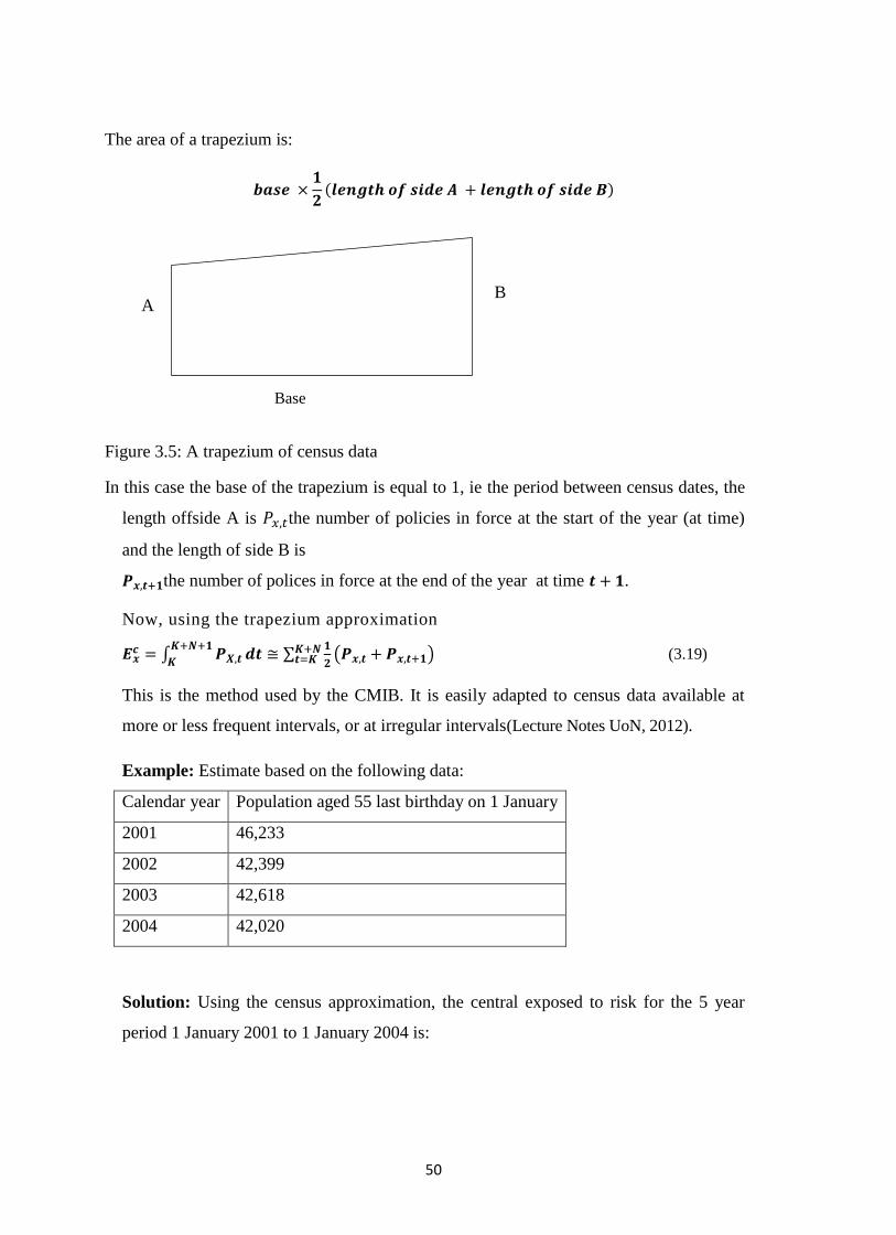
50
The area of a trapezium is:
Figure 3.5: A trapezium of census data
In this case the base of the trapezium is equal to 1, ie the period between census dates, the
length offside A is the number of policies in force at the start of the year (at time)
and the length of side B is
the number of polices in force at the end of the year at time .
Now, using the trapezium approximation
(3.19)
This is the method used by the CMIB. It is easily adapted to census data available at
more or less frequent intervals, or at irregular intervals(Lecture Notes UoN, 2012).
Example: Estimate based on the following data:
Calendar year Population aged 55 last birthday on 1 January
2001 46,233
2002 42,399
2003 42,618
2004 42,020
Solution: Using the census approximation, the central exposed to risk for the 5 year
period 1 January 2001 to 1 January 2004 is:
B A
Base
51
3.11 Estimating transition intensities
Define as the number of transitions from state i to state j , and let denote the
"waiting time" in state i . These random variables have realizations depending
on whether we are discussing estimators or estimates) (Scott W.F.1991). We state the
following important results: that the vector is the maximum likelihood estimator of
the true value, and that the asymptotic distribution of the vector of maximum
likelihood estimators is multivariate Normal with mean equal to the vector of true
transition intensities, the variance matrix has diagonal elements(Lecture Notes UoN,
2012).
and off-diagonal elements zero. Hence the asymptotic distribution of the
component
.
Now the asymptotic posterior distribution of is approximately
(Scott W.F., 1991).
We now label the N lives from k = 1 to k = N , since the symbol i may be used to index
the states. We can use an example to illustrate the methodology: In a certain
investigation, 40 "active" lives become "ill" and there were 8,176 years of exposure
among the "active" lives. (Some "ill" lives recovered, and some of the "active" lives and
"ill" lives died). Estimate the force of transition from the "active" to the "ill" state (this
being assumed to be the same at all ages) and give an approximate 95% confidence
interval(Scott W.F.1991).
52
The solution will be as follows:
is the M.L.E. of . The estimated s.d. of is
so an approximate 95% confidence interval for is
(Scott W.F., 1991).
3.12 Graduation by Parametric Formula
There are usually three methods of carrying out a graduation which are graduation by
parametric formula, graduation by reference to a standard table and graphical graduation
(Lecture notes, UoN, 2012). The most appropriate method of graduation to use will depend on
the quality of the data available and the purpose for which the graduated rates will be used.
The general methodology of graduation is essentially the same under each method. Once we
have decided on the appropriate method, we will choose a model of represent the underlying
force (or rates) of mortality or transition, fit the model to the crude observed rates and test the
graduation for adherence to data and ( if necessary) smoothness. Each method can produce
many possible graduations. The graduation chosen will be the one whose adherence and
smoothness best meet the requirements for which the rates are intended(Lecture Notes UoN,
2012).
Graduation is a compromise between adherence to data (goodness of fit) and smoothness. The
balance that we want between these two conflicting objectives is a subjective choice and will
depend on how the graduated rates will be used. For example if we are constructing a standard
table of national population mortality, we will be interested in maximizing the accuracy. We
will put more emphasis on adherence and less emphasis on smoothness. If the rates are to be
used to calculate premiums and reserves for a life insurance company, we will want to ensure
that the rates (and hence the premiums and reserves) progress smoothly from age to age to avoid
sudden changes and inconsistencies. We will put more emphasis on smoothness and less
emphasis on adherence. The mortality rates at ages around the accident hump will be less
important in this situation are few policy holders are likely to be in the age range 18-22 years.
In this study however, we will focus on graduation by formula because of its pragmatic nature.
53
The method of graduation most often used for reasonably large experiences is to fit a parametric
formula to the crude estimates(London, D. 1985).
The underlying assumption is (or ) can be modeled using an appropriate mathematical
formula with unknown parameters. The parameters are typically calculated automatically by a
computer using numerical methods.
If the formula used does not include enough parameters, it will not be flexible enough to follow
the crude rates closely, which may result in over graduation. If too many parameters are
included, sudden bends may appear in the graduated curve, which may result in under
graduation.
For different values of the parameters, we can assess the smoothness and adherence to data of
the fitted model. (In practice we will not need to check smoothness if the number of parameters
is sufficiently small).
We will choose the values of the parameters that provide the most appropriate model, according
to some pre-defined criterion in respect of goodness of fit. Two simple (but useful) formulae
are:
Gompertz (1825) = (3.20)
Makeham (1860) = A + Bc2(66)
(Scott W.F., 1999)
In practice, it is usually found that follows an exponential curve quite closely over middle
and older ages (in human populations) so most successful formulae include a Gompertz term.
Makeham’s formula is interpreted as the addition of accidental deaths, independent of age, to a
Gompertz term representing senescent deaths.
The most recent standard tables produced for us by UK life insurance companies used formulae
of the form.
= pollynomial1 + exp (polyinomial2)
Which includes Gompertz and Makeham as special cases(London, D. 1985). The formulae were
of the form:
=f ( Where
Polynomial (1) = + x + x2 + …. + xr -1
54
Polynomial (2)= + + + ….
In other words, a formula with (r +s) parameters was fitted for each table of the form =
polynomial1 + exp (polynomial2).
The researcher chose to use a Perks formula specification, a(x), to graduate transition
intensities to sickness states. Moreover, an additional parameter, H, was included for
the purposes of a more suitable fit.
HKcDc
BcAxa
xx
x
1)( (3.21)
Graduations using the Gompertz-Makeham and Logit Gompertz-Makeham formula of
type (r,s) have been investigated previously using health and disability related data (
CMIR 6 (1983) and CMIR 17 (1991)). Generally, the LogitGompertz-Makeham
formula is expressed as:
)(1
)()(
5,
5,
5,
xGM
xGMxLGM
r
r
r
Where
r
i
r
ri
ri
i
i
i
r xxxGM1
5
1
115, exp)(
(5.21)
is the Gompertz-Makeham formula of type (r,s) (Forfar et al 1985).
A LogitGompertz-Makeham formula, LG M ( 1 , 2 ) , was found to fit sufficiently well
here for recovery intensities, that is:
)exp(1
)exp(
321
3210
x
xji
x
(3.22)
3.13 Calculation of Premiums using the equivalence principle
So far we have shown that multiple state models are a natural way of modeling cash
flows for insurance policies and we have also shown how to evaluate probabilities for
such models given only the transition intensities between pairs of states. The next stage
in our study of multiple state models is to calculate premiums and policy values for a
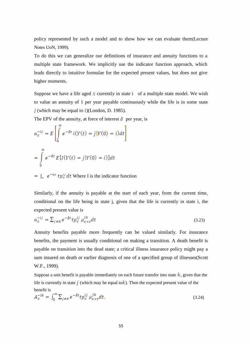
55
policy represented by such a model and to show how we can evaluate them(Lecture
Notes UoN, 1999).
To do this we can generalize our definitions of insurance and annuity functions to a
multiple state framework. We implicitly use the indicator function approach, which
leads directly to intuitive formulae for the expected present values, but does not give
higher moments.
Suppose we have a life aged currently in state i of a multiple state model. We wish
to value an annuity of 1 per year payable continuously while the life is in some state
(which may be equal to )(London, D. 1985).
The EPV of the annuity, at force of interest per year, is
Where I is the indicator function
Similarly, if the annuity is payable at the start of each year, from the current time,
conditional on the life being in state j, given that the life is currently in state i, the
expected present value is
(3.23)
Annuity benefits payable more frequently can be valued similarly. For insurance
benefits, the payment is usually conditional on making a transition. A death benefit is
payable on transition into the dead state; a critical illness insurance policy might pay a
sum insured on death or earlier diagnosis of one of a specified group of illnesses(Scott
W.F., 1999).
Suppose a unit benefit is payable immediately on each future transfer into state , given that the
life is currently in state (which may be equal to ). Then the expected present value of the
benefit is
. (3.24)

56
To derive this, we consider payment in the interval so that the amount of the
payment is 1, the discount factor (for sufficiently small dt)is, and the probability
that the benefit is paid is the probability that the life transfers into state k in
given that the life is in state at time 0. In order to transfer into state k in the
life must be in some state j that is not immediately before (the probability of two
transitions in infinitesimal time being negligible), with probability then transfer
from j to k during the interval with probability . Summing (that is,
integrating) over all the possible time intervals gives equation (3.24).
Other benefits and annuity designs are feasible; for example, a lump sum benefit might
be paid on the first transition from healthy to sick, or premiums may be paid only during
the first sojourn in state 0. Most practical cases can be managed from first principles
using the indicator function approach(Lecture Notes UoN, 2012).
In general, premiums are calculated using the equivalence principle and we assume that
lives are in state 0 at the policy inception date(London, D. 1985).
Example 3.1: Suppose an insurer issues a 10-year disability income insurance policy to
a healthy life aged 60. Calculate the premiums for the following two policy designs
using the model and parameters given from Example: Assume an interest rate of 5% per
year effective, and that there are no expenses.
(a) Premiums are payable continuously while in the healthy state. A benefit of $20000
per year is payable continuously while in the disabled state. A death benefit of $50000
is payable immediately on death.
(b) Premiums are payable monthly in advance conditional on the life being in the
healthy state at the premium date. The sickness benefit of $20000 per year is
payable monthly in arrear, if the life is in the sick state at the payment date. A death
benefit of $50000 is payable immediately on death(Dickson et al, 2009)..
Solution :(a) We equate the EPV of the premiums with the EFV of the benefits.
The computation of the EPV of the benefits requires numerical integration. All values
below have been calculated using the repeated Simpson's rule, with h = 1/12. Using
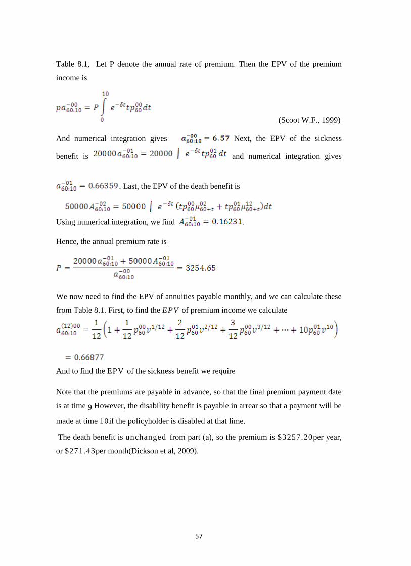
57
Table 8.1, Let P denote the annual rate of premium. Then the EPV of the premium
income is
(Scoot W.F., 1999)
And numerical integration gives Next, the EPV of the sickness
benefit is and numerical integration gives
. Last, the EPV of the death benefit is
Using numerical integration, we find .
Hence, the annual premium rate is
We now need to find the EPV of annuities payable monthly, and we can calculate these
from Table 8.1. First, to find the EPV of premium income we calculate
And to find the EPV of the sickness benefit we require
Note that the premiums are payable in advance, so that the final premium payment date
is at time 9 However, the disability benefit is payable in arrear so that a payment will be
made at time 10if the policyholder is disabled at that lime.
The death benefit is unchanged from part (a), so the premium is $3257.20per year,
or $271.43per month(Dickson et al, 2009).

58
3.14 Policy values or Reserves and Thiele's differential equation
The definition of the time t policy value for a policy modeled using a multiple
state model is the expected value at that time
of the future loss random variable - with one additional requirement. For a
policy described by a multiple state model, the future loss random variable, and
hence the policy value, at duration t years depends on which state of the model the
policyholder is in at that time. We can express this formally as follows: a policy value is
the expected value at that time of the future loss random variable conditional on the
policy being in a given state at that time(Dickson et al, 2009). We use the following
notation for policy values(Scott W.F.1991).
Notation)(itV denotes the policy value at duration t for a policy which is in state i at that
time. A policy value depends numerically on the basis used in its calculation, that is the
transition intensities between pairs of states as functions of the individual’s age, the
force of interest, the assumed expenses, and the assumed bonus rates in the case of
participating policies. The key to calculating policy values is Thiele’s differential
equation, which can be solved numerically using Euler’s method(Dickson et al, 2009).
Notation, )(itV denotes the policy value at duration t for a policy which is in state i at
that time. The key to calculating policy values is Thiele's differential equation, which
can be solved numerically using Euler's, or some more sophisticated, method. To
establish some ideas we start by considering the disability income insurance model.
Suppose we consider a policy with a term of n years issued to a life aged x. Premiums
are payable continuously throughout the term at rate P per year while the life is healthy,
an annuity benefit is payable continuously at rate B per year while the life is sick, and a
lump sum, 5, is payable immediately on death within the term. Recovery from sick to
healthy is possible and the disability income insurance model is appropriate(Scoot W.F.,
1999). We are interested in calculating policy values for this policy and also in
calculating the premium using the equivalence principle. For simplicity we ignore
expenses in this section, but these could be included as extra 'benefits' or negative
'premiums' provided only that they are payable continuously at a constant rate while the
life is in a given state and/or are payable as lump sums immediately on transition
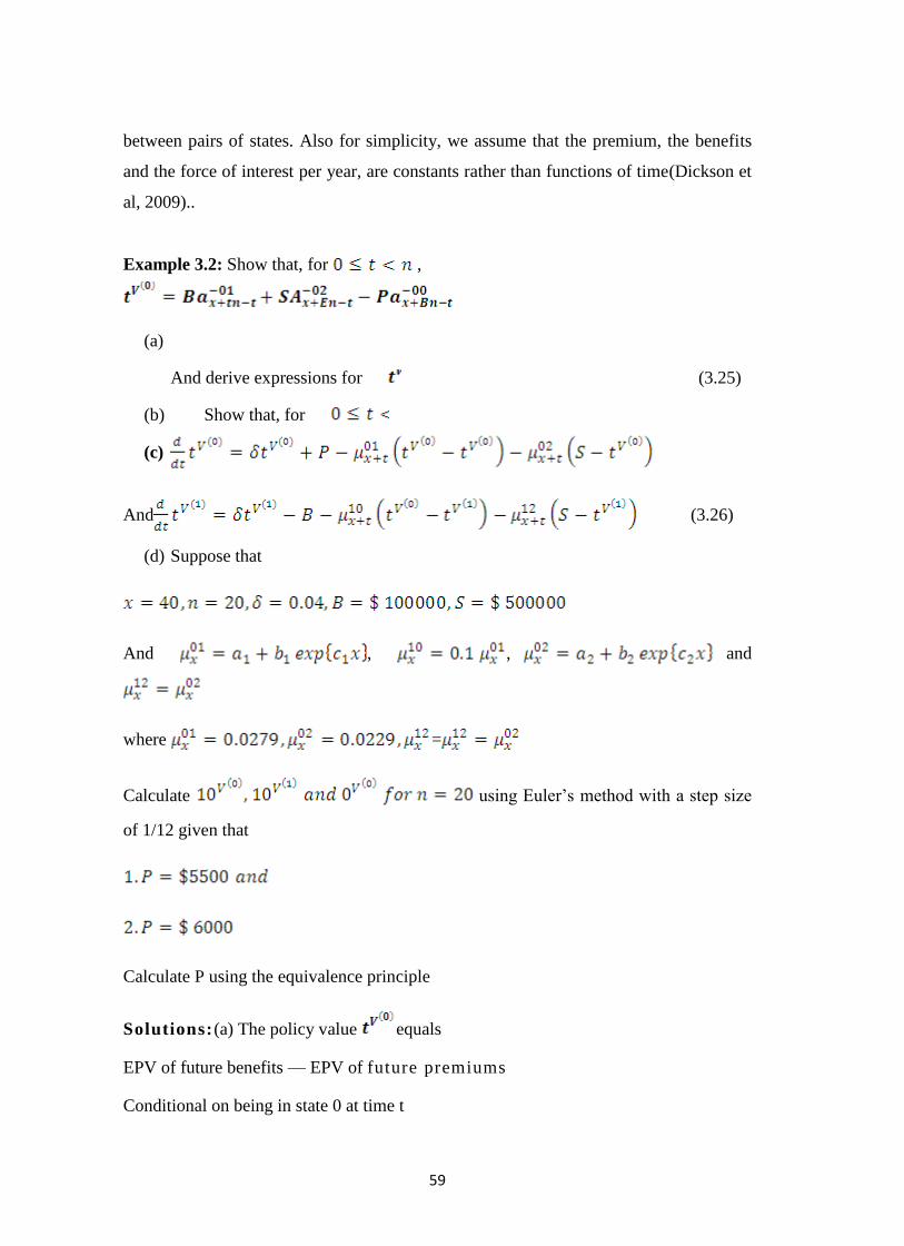
59
between pairs of states. Also for simplicity, we assume that the premium, the benefits
and the force of interest per year, are constants rather than functions of time(Dickson et
al, 2009)..
Example 3.2: Show that, for ,
(a)
And derive expressions for (3.25)
(b) Show that, for
(c)
And (3.26)
(d) Suppose that
And , , and
where =
Calculate using Euler’s method with a step size
of 1/12 given that
Calculate P using the equivalence principle
Solutions:(a) The policy value equals
EPV of future benefits — EPV of future premiums
Conditional on being in state 0 at time t
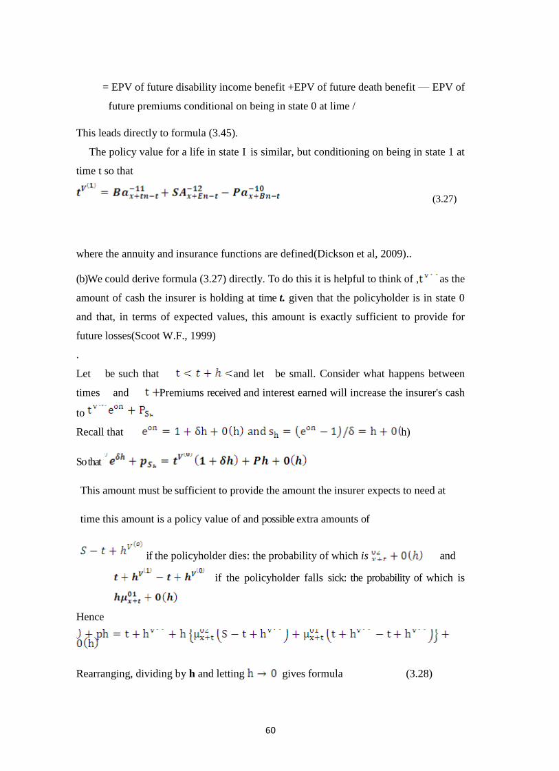
60
= EPV of future disability income benefit +EPV of future death benefit — EPV of
future premiums conditional on being in state 0 at lime /
This leads directly to formula (3.45).
The policy value for a life in state I is similar, but conditioning on being in state 1 at
time t so that
(3.27)
where the annuity and insurance functions are defined(Dickson et al, 2009)..
(b)We could derive formula (3.27) directly. To do this it is helpful to think of , as the
amount of cash the insurer is holding at time t. given that the policyholder is in state 0
and that, in terms of expected values, this amount is exactly sufficient to provide for
future losses(Scoot W.F., 1999)
.
Let be such that and let be small. Consider what happens between
times and Premiums received and interest earned will increase the insurer's cash
to
Recall that h)
So that
This amount must be sufficient to provide the amount the insurer expects to need at
time this amount is a policy value of and possible extra amounts of
if the policyholder dies: the probability of which is and
if the policyholder falls sick: the probability of which is
Hence
Rearranging, dividing by h and letting gives formula (3.28)
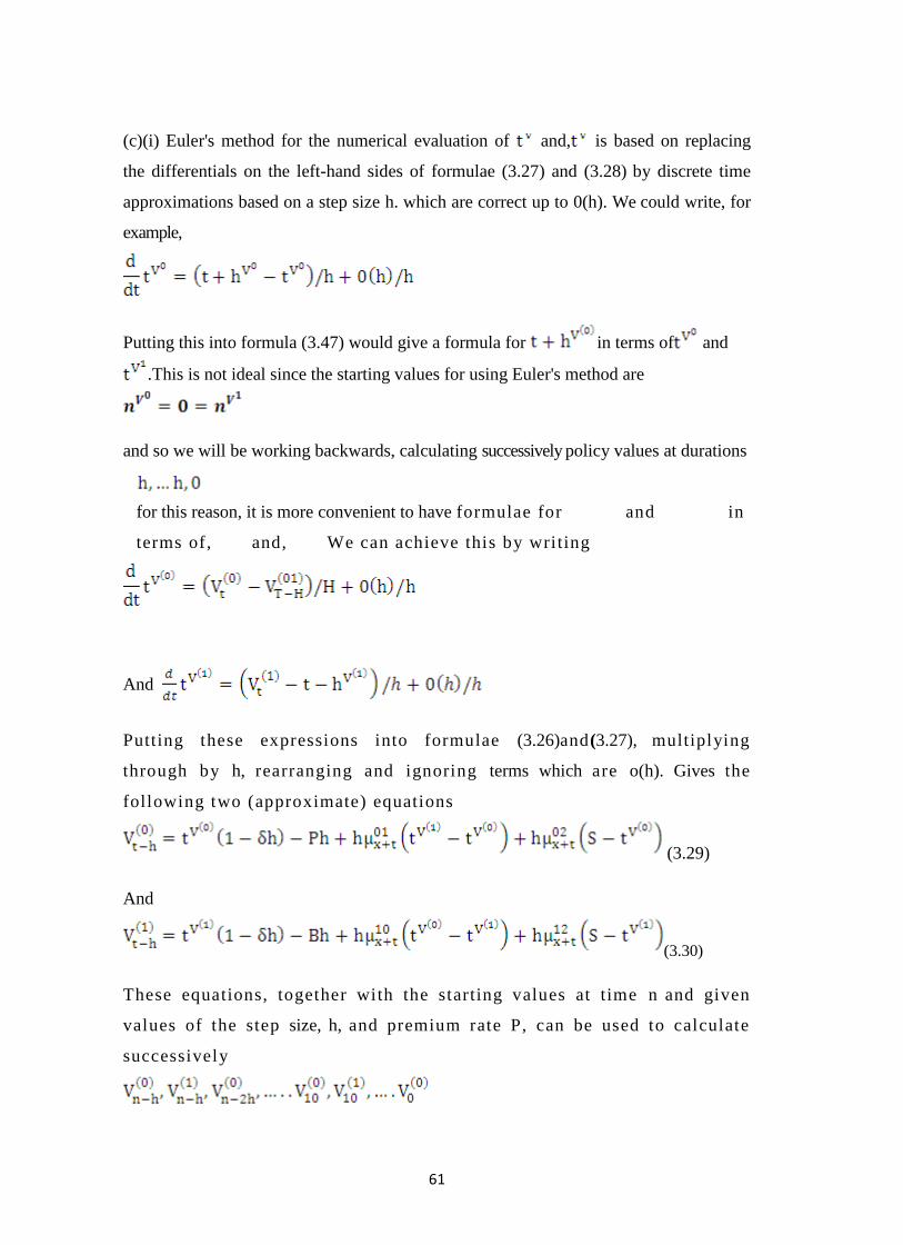
61
(c)(i) Euler's method for the numerical evaluation of and, is based on replacing
the differentials on the left-hand sides of formulae (3.27) and (3.28) by discrete time
approximations based on a step size h. which are correct up to 0(h). We could write, for
example,
Putting this into formula (3.47) would give a formula for in terms of and
.This is not ideal since the starting values for using Euler's method are
and so we will be working backwards, calculating successively policy values at durations
for this reason, it is more convenient to have formulae for and in
terms of, and, We can achieve this by writing
And
Putting these expressions into formulae (3.26)and(3.27), multiplying
through by h, rearranging and ignoring terms which are o(h). Gives the
following two (approximate) equations
(3.29)
And
(3.30)
These equations, together with the starting values at time n and given
values of the step size, h, and premium rate P, can be used to calculate
successively
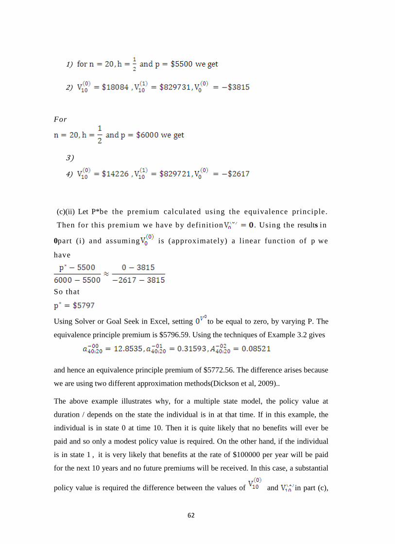
62
1)
2)
For
3)
4)
(c)(ii) Let P*be the premium calculated using the equivalence principle.
Then for this premium we have by definit ion . Using the results in
0part (i) and assuming is (approximately) a linear function of p we
have
So that
Using Solver or Goal Seek in Excel, setting to be equal to zero, by varying P. The
equivalence principle premium is $5796.59. Using the techniques of Example 3.2 gives
and hence an equivalence principle premium of $5772.56. The difference arises because
we are using two different approximation methods(Dickson et al, 2009)..
The above example illustrates why, for a multiple state model, the policy value at
duration / depends on the state the individual is in at that time. If in this example, the
individual is in state 0 at time 10. Then it is quite likely that no benefits will ever be
paid and so only a modest policy value is required. On the other hand, if the individual
is in state 1 , it is very likely that benefits at the rate of $100000 per year will be paid
for the next 10 years and no future premiums will be received. In this case, a substantial
policy value is required the difference between the values of and in part (c),
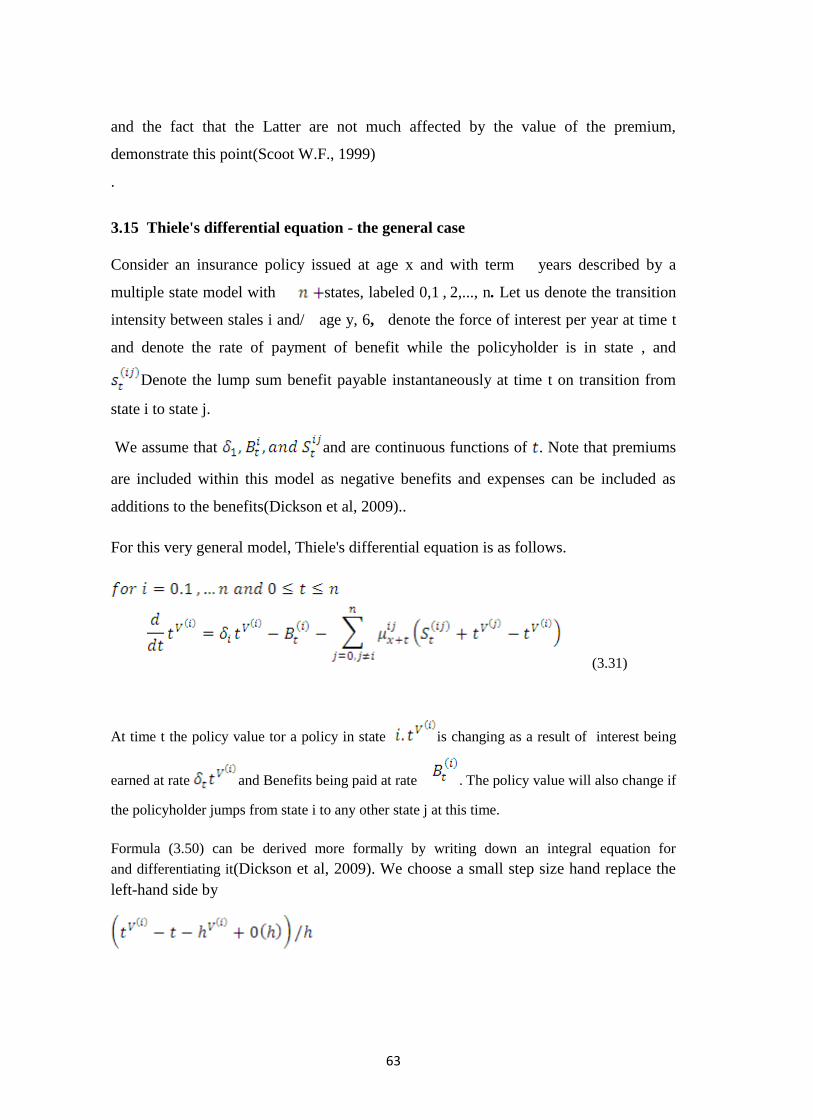
63
and the fact that the Latter are not much affected by the value of the premium,
demonstrate this point(Scoot W.F., 1999)
.
3.15 Thiele's differential equation - the general case
Consider an insurance policy issued at age x and with term years described by a
multiple state model with states, labeled 0,1 , 2,..., n. Let us denote the transition
intensity between stales i and/ age y, 6, denote the force of interest per year at time t
and denote the rate of payment of benefit while the policyholder is in state , and
Denote the lump sum benefit payable instantaneously at time t on transition from
state i to state j.
We assume that and are continuous functions of . Note that premiums
are included within this model as negative benefits and expenses can be included as
additions to the benefits(Dickson et al, 2009)..
For this very general model, Thiele's differential equation is as follows.
(3.31)
At time t the policy value tor a policy in state is changing as a result of interest being
earned at rate and Benefits being paid at rate . The policy value will also change if
the policyholder jumps from state i to any other state j at this time.
Formula (3.50) can be derived more formally by writing down an integral equation for and differentiating it(Dickson et al, 2009). We choose a small step size hand replace the
left-hand side by
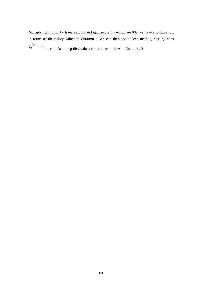
64
Multiplying through by h rearranging and ignoring terms which are 0(h),we have a formula for.
in terms of the policy values at duration t. We can then use Euler's method, starting with
to calculate the policy values at durations

65
CHAPTER FOUR: APPLICATIONS, DATA PRESENTATION AND ANALYSIS
4.1 Introduction
In Kenya, the lack of a scientifically modeled national health financing insurance can be
attributed to the lack of complete, comprehensive and reliable data. This is particularly
problematic in the case of LTC insurance given the unusually broad range of services
and modes of disability associated with LTC (Eagles 1992). Clearly choice of data will
influence the modeling methodology. In this chapter, therefore, a case study of National
Hospital Insurance Fund (N.H.I.F.) is undertaken for the purposes of both introducing
the current and available data sets in Kenya and, more importantly, in justifying the
choice of data used in this project. The choice of N.H.I.F. was particularly informed by
the fact it is the only LTC insurer with a scheme of more than 200,000 principal
members. Other private insurers have schemes in tens of thousands which the researcher
found to be insufficient for the purpose of multi state modeling.
4.2 Data Requirements
Ideal data for LTC insurance pricing is a longitudinal data set that tracks both levels of
disability and LTC utilization patterns of a large representative population. As discussed
by Meiners (1989), the benefit of longitudinal data for LTC pricing is primarily to
enable an understanding of LTC utilization changes as the cohort ages.
Many nations, including Kenya, lack a systematic LTC data-reporting program enabling
comprehensive information to be collected across service sectors, care programs and
jurisdictions (Reif 1985). Given that Kenya currently has no private insurance coverage
for LTC, there is clearly a need to gather data on virtually all aspects of LTC insurance
covers including costs, risk management, marketing and underwriting. From a pure
actuarial pricing and reserving perspective, utilization/demand data for LTC segregated
by age and sex in conjunction with changes to utilization(ie functional changes) as a
function of age are essential. The following sections discuss and evaluate the various
options for obtaining this information.
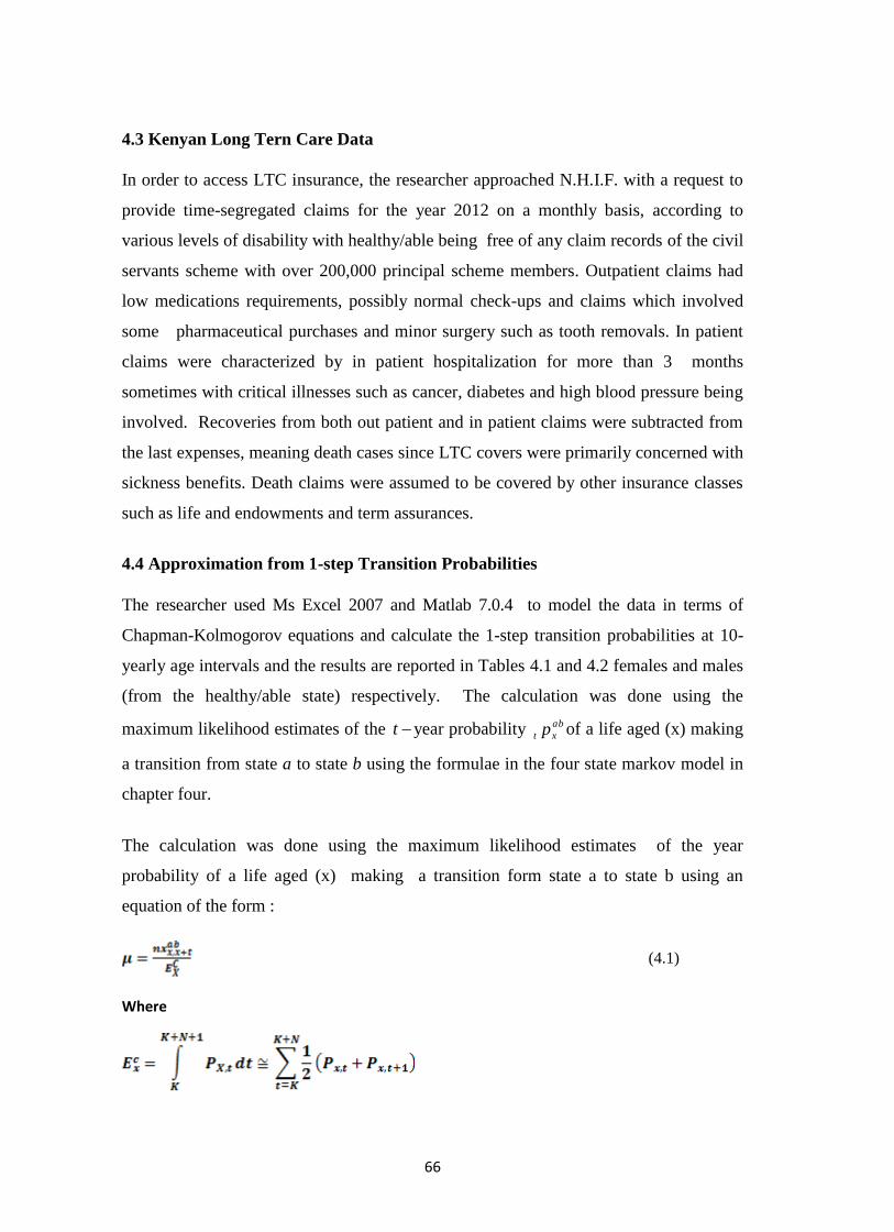
66
4.3 Kenyan Long Tern Care Data
In order to access LTC insurance, the researcher approached N.H.I.F. with a request to
provide time-segregated claims for the year 2012 on a monthly basis, according to
various levels of disability with healthy/able being free of any claim records of the civil
servants scheme with over 200,000 principal scheme members. Outpatient claims had
low medications requirements, possibly normal check-ups and claims which involved
some pharmaceutical purchases and minor surgery such as tooth removals. In patient
claims were characterized by in patient hospitalization for more than 3 months
sometimes with critical illnesses such as cancer, diabetes and high blood pressure being
involved. Recoveries from both out patient and in patient claims were subtracted from
the last expenses, meaning death cases since LTC covers were primarily concerned with
sickness benefits. Death claims were assumed to be covered by other insurance classes
such as life and endowments and term assurances.
4.4 Approximation from 1-step Transition Probabilities
The researcher used Ms Excel 2007 and Matlab 7.0.4 to model the data in terms of
Chapman-Kolmogorov equations and calculate the 1-step transition probabilities at 10-
yearly age intervals and the results are reported in Tables 4.1 and 4.2 females and males
(from the healthy/able state) respectively. The calculation was done using the
maximum likelihood estimates of the t year probability ab
xt p of a life aged (x) making
a transition from state a to state b using the formulae in the four state markov model in
chapter four.
The calculation was done using the maximum likelihood estimates of the year
probability of a life aged (x) making a transition form state a to state b using an
equation of the form :
(4.1)
Where
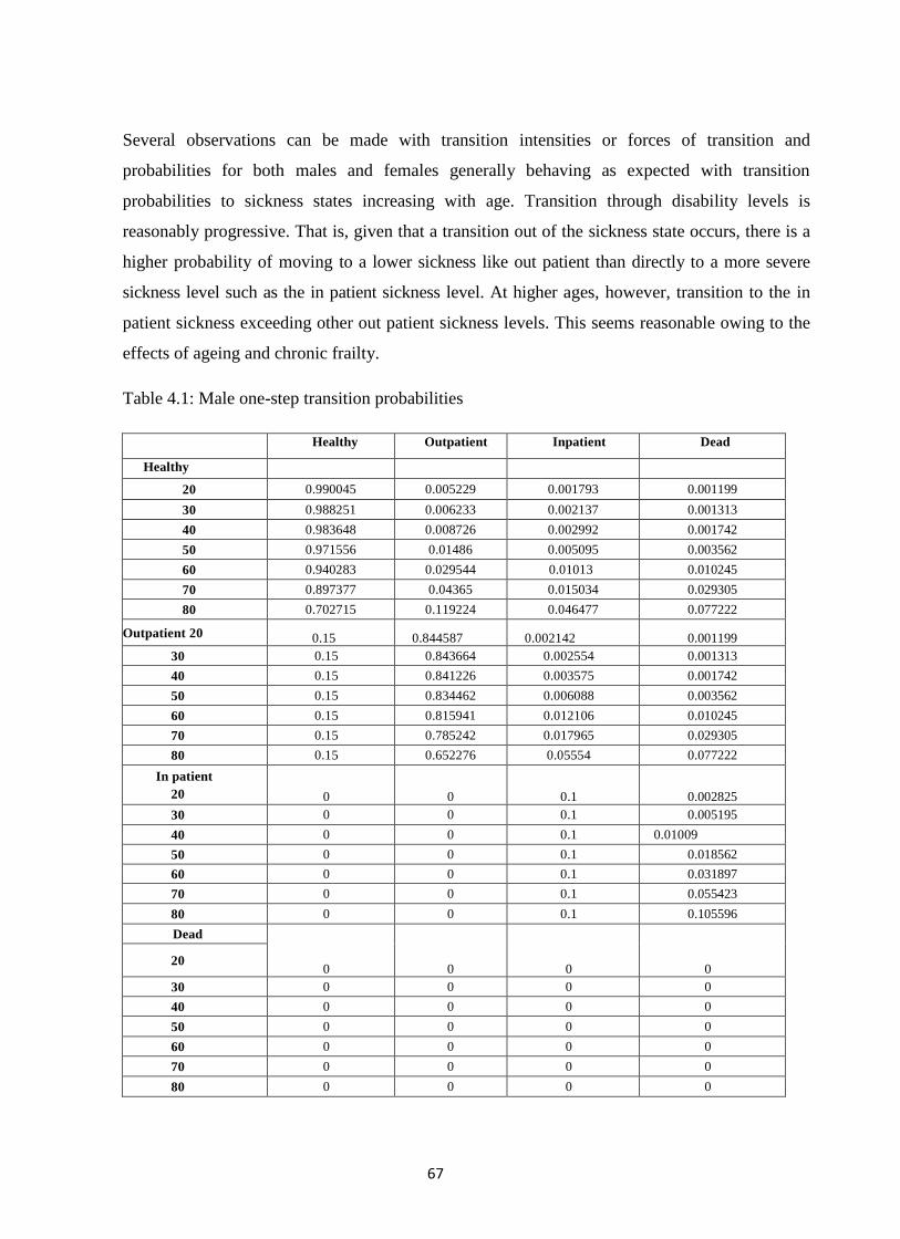
67
Several observations can be made with transition intensities or forces of transition and
probabilities for both males and females generally behaving as expected with transition
probabilities to sickness states increasing with age. Transition through disability levels is
reasonably progressive. That is, given that a transition out of the sickness state occurs, there is a
higher probability of moving to a lower sickness like out patient than directly to a more severe
sickness level such as the in patient sickness level. At higher ages, however, transition to the in
patient sickness exceeding other out patient sickness levels. This seems reasonable owing to the
effects of ageing and chronic frailty.
Table 4.1: Male one-step transition probabilities
Healthy Outpatient Inpatient Dead
Healthy
20 0.990045 0.005229 0.001793 0.001199
30 0.988251 0.006233 0.002137 0.001313
40 0.983648 0.008726 0.002992 0.001742
50 0.971556 0.01486 0.005095 0.003562
60 0.940283 0.029544 0.01013 0.010245
70 0.897377 0.04365 0.015034 0.029305
80 0.702715 0.119224 0.046477 0.077222
Outpatient 20 0.15 0.844587 0.002142 0.001199
30 0.15 0.843664 0.002554 0.001313
40 0.15 0.841226 0.003575 0.001742
50 0.15 0.834462 0.006088 0.003562
60 0.15 0.815941 0.012106 0.010245
70 0.15 0.785242 0.017965 0.029305
80 0.15 0.652276 0.05554 0.077222
In patient
20 0 0 0.1 0.002825
30 0 0 0.1 0.005195
40 0 0 0.1 0.01009
50 0 0 0.1 0.018562
60 0 0 0.1 0.031897
70 0 0 0.1 0.055423
80 0 0 0.1 0.105596
Dead
0 0 0 0 20
30 0 0 0 0
40 0 0 0 0
50 0 0 0 0
60 0 0 0 0
70 0 0 0 0
80 0 0 0 0
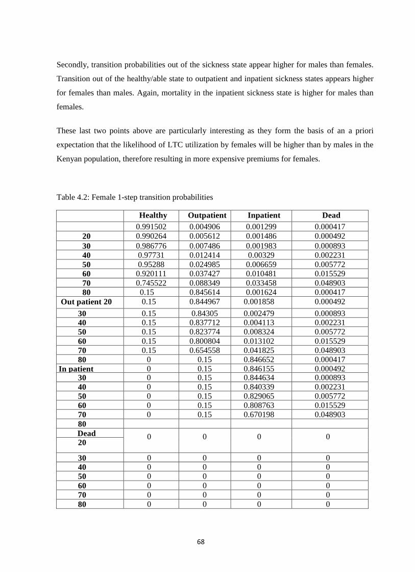
68
Secondly, transition probabilities out of the sickness state appear higher for males than females.
Transition out of the healthy/able state to outpatient and inpatient sickness states appears higher
for females than males. Again, mortality in the inpatient sickness state is higher for males than
females.
These last two points above are particularly interesting as they form the basis of an a priori
expectation that the likelihood of LTC utilization by females will be higher than by males in the
Kenyan population, therefore resulting in more expensive premiums for females.
Table 4.2: Female 1-step transition probabilities
Healthy Outpatient Inpatient Dead
Healthy
0.991502 0.004906 0.001299 0.000417
20 0.990264 0.005612 0.001486 0.000492
30 0.986776 0.007486 0.001983 0.000893
40 0.97731 0.012414 0.00329 0.002231
50 0.95288 0.024985 0.006659 0.005772
60 0.920111 0.037427 0.010481 0.015529
70 0.745522 0.088349 0.033458 0.048903
80 0.15 0.845614 0.001624 0.000417
Out patient 20 0.15 0.844967 0.001858 0.000492
30 0.15 0.84305 0.002479 0.000893
40 0.15 0.837712 0.004113 0.002231
50 0.15 0.823774 0.008324 0.005772
60 0.15 0.800804 0.013102 0.015529
70 0.15 0.654558 0.041825 0.048903
80 0 0.15 0.846652 0.000417
In patient
20
0 0.15 0.846155 0.000492 30 0 0.15 0.844634 0.000893
40 0 0.15 0.840339 0.002231
50 0 0.15 0.829065 0.005772
60 0 0.15 0.808763 0.015529
70 0 0.15 0.670198 0.048903
80
Dead 0 0 0 0 20
30 0 0 0 0
40 0 0 0 0
50 0 0 0 0
60 0 0 0 0
70 0 0 0 0
80 0 0 0 0
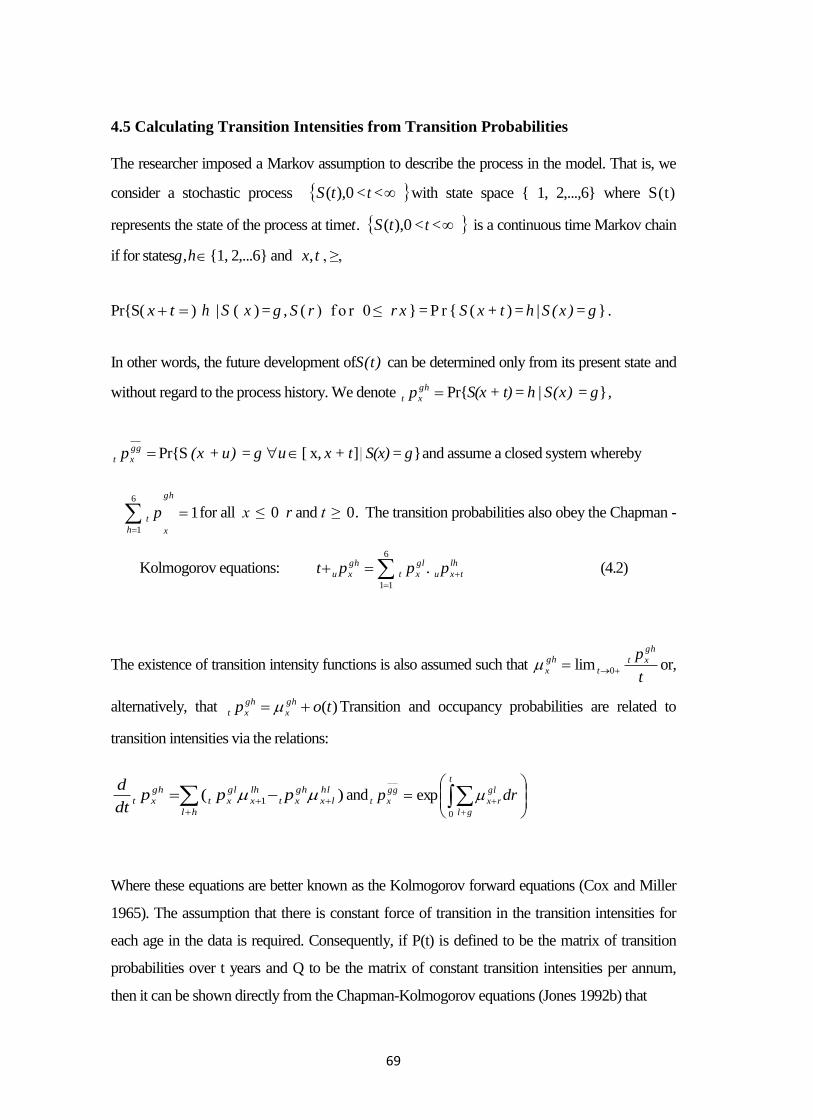
69
4.5 Calculating Transition Intensities from Transition Probabilities
The researcher imposed a Markov assumption to describe the process in the model. That is, we
consider a stochastic process 0),(tS < t < with state space { 1, 2,...,6} where S(t)
represents the state of the process at timet. 0),(tS < t < is a continuous time Markov chain
if for statesg,h{1, 2,...6} and tx, , ≥,
Pr{S( tx ) h | S ( x ) = g , S ( r ) f o r 0 ≤ r x } = P r { S ( x + t ) = h | S (x )=g } .
In other words, the future development ofS(t) can be determined only from its present state and
without regard to the process history. We denote gh
xt p Pr{S(x + t) = h | S(x) = g},
gg
xt p Pr{S (x + u) = g u [ x, x + t] | S(x) = g}and assume a closed system whereby
16
1
gh
xh
t p for all x ≤ 0 r and t ≥ 0. The transition probabilities also obey the Chapman -
Kolmogorov equations:
6
11
. lh
txu
gl
xt
gh
xu pppt (4.2)
The existence of transition intensity functions is also assumed such that t
p gh
xtt
gh
x 0lim or,
alternatively, that )(top gh
x
gh
xt Transition and occupancy probabilities are related to
transition intensities via the relations:
)( 1
hl
lx
gh
xt
lh
x
gl
xt
hl
gh
xt pppdt
d
and
t
gl
gl
rx
gg
xt drp0
exp
Where these equations are better known as the Kolmogorov forward equations (Cox and Miller
1965). The assumption that there is constant force of transition in the transition intensities for
each age in the data is required. Consequently, if P(t) is defined to be the matrix of transition
probabilities over t years and Q to be the matrix of constant transition intensities per annum,
then it can be shown directly from the Chapman-Kolmogorov equations (Jones 1992b) that
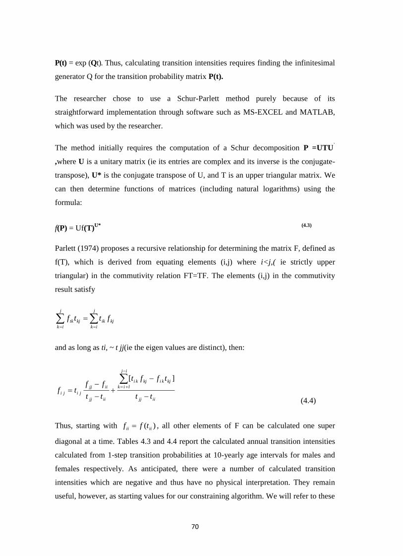
70
P(t) = exp (Qt). Thus, calculating transition intensities requires finding the infinitesimal
generator Q for the transition probability matrix P(t).
The researcher chose to use a Schur-Parlett method purely because of its
straightforward implementation through software such as MS-EXCEL and MATLAB,
which was used by the researcher.
The method initially requires the computation of a Schur decomposition P =UTU`
,where U is a unitary matrix (ie its entries are complex and its inverse is the conjugate-
transpose), U* is the conjugate transpose of U, and T is an upper triangular matrix. We
can then determine functions of matrices (including natural logarithms) using the
formula:
f(P) = Uf(T)U* (4.3)
Parlett (1974) proposes a recursive relationship for determining the matrix F, defined as
f(T), which is derived from equating elements (i,j) where i<j,( ie strictly upper
triangular) in the commutivity relation FT=TF. The elements (i,j) in the commutivity
result satisfy
j
ik
j
ik
kjikkjtk fttf
and as long as ti, ~ t jj(ie the eigen values are distinct), then:
iijj
ij
lik
kjkikjki
iijj
iijj
jijitt
tfft
tt
fftf
][
(4.4)
Thus, starting with )( iiii tff , all other elements of F can be calculated one super
diagonal at a time. Tables 4.3 and 4.4 report the calculated annual transition intensities
calculated from 1-step transition probabilities at 10-yearly age intervals for males and
females respectively. As anticipated, there were a number of calculated transition
intensities which are negative and thus have no physical interpretation. They remain
useful, however, as starting values for our constraining algorithm. We will refer to these
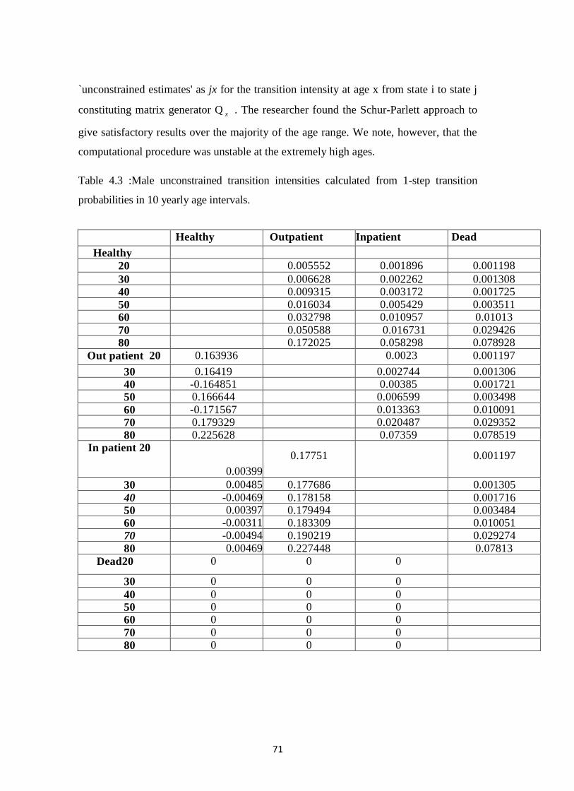
71
`unconstrained estimates' as jx for the transition intensity at age x from state i to state j
constituting matrix generator Q x . The researcher found the Schur-Parlett approach to
give satisfactory results over the majority of the age range. We note, however, that the
computational procedure was unstable at the extremely high ages.
Table 4.3 :Male unconstrained transition intensities calculated from 1-step transition
probabilities in 10 yearly age intervals.
Healthy Outpatient Inpatient Dead
Healthy
20 0.005552 0.001896 0.001198
30 0.006628 0.002262 0.001308
40 0.009315 0.003172 0.001725
50 0.016034 0.005429 0.003511
60 0.032798 0.010957 0.01013
70 0.050588 0.016731 0.029426 80 0.172025 0.058298 0.078928
Out patient 20 0.163936 0.0023 0.001197
30 0.16419 0.002744 0.001306
40 -0.164851 0.00385 0.001721
50 0.166644 0.006599 0.003498
60 -0.171567 0.013363 0.010091
70 0.179329 0.020487 0.029352
80 0.225628 0.07359 0.078519
In patient 20
20
0.00399
0.17751 0.001197
30 0.00485 0.177686 0.001305
40 -0.00469 0.178158 0.001716
50 0.00397 0.179494 0.003484
60 -0.00311 0.183309 0.010051
70 -0.00494 0.190219 0.029274
80 0.00469 0.227448 0.07813
Dead20
20
0 0 0
30 0 0 0
40 0 0 0 50 0 0 0
60 0 0 0
70 0 0 0
80 0 0 0
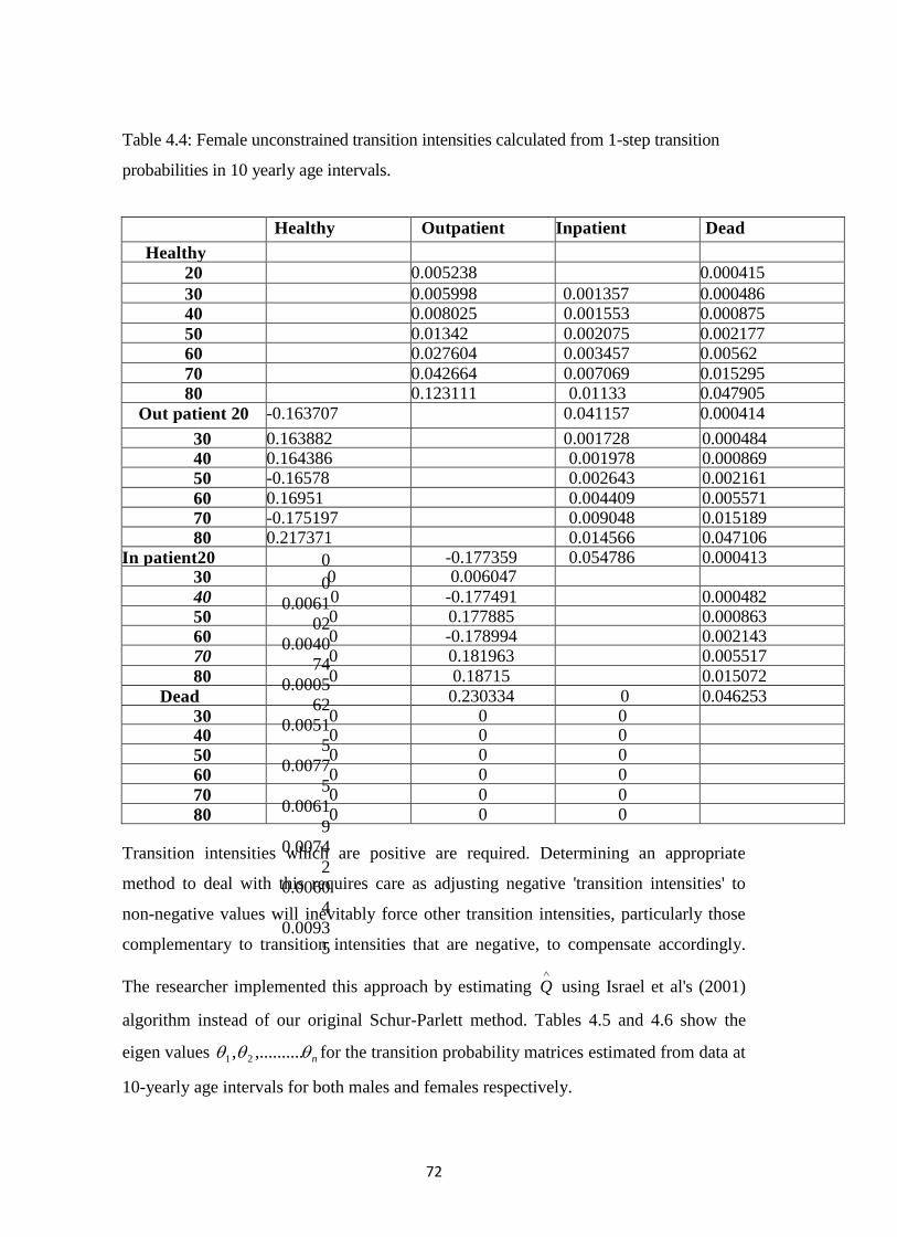
72
Table 4.4: Female unconstrained transition intensities calculated from 1-step transition
probabilities in 10 yearly age intervals.
Healthy Outpatient Inpatient Dead
Healthy
20 0.005238 0.000415
30 0.005998 0.001357 0.000486
40 0.008025 0.001553 0.000875
50 0.01342 0.002075 0.002177
60 0.027604 0.003457 0.00562
70 0.042664 0.007069 0.015295
80 0.123111 0.01133 0.047905
Out patient 20 -0.163707 0.041157 0.000414
30 0.163882 0.001728 0.000484
40 0.164386 0.001978 0.000869
50 -0.16578 0.002643 0.002161
60 0.16951 0.004409 0.005571
70 -0.175197 0.009048 0.015189
80 0.217371 0.014566 0.047106
In patient20
20
0
0
0.0061
02
0.0040
74
0.0005
62
0.0051
5
0.0077
5
0.0061
9
0.0074
2
0.0060
4
0.0093
5
-0.177359 0.054786 0.000413 30 0 0.006047
40 0 -0.177491 0.000482
50 0 0.177885 0.000863
60 0 -0.178994 0.002143
70 0 0.181963 0.005517
80 0 0.18715 0.015072
Dead
20
0.230334 0 0.046253
30 0 0 0 40 0 0 0
50 0 0 0
60 0 0 0
70 0 0 0
80 0 0 0
Transition intensities which are positive are required. Determining an appropriate
method to deal with this requires care as adjusting negative 'transition intensities' to
non-negative values will inevitably force other transition intensities, particularly those
complementary to transition intensities that are negative, to compensate accordingly.
The researcher implemented this approach by estimating
Q using Israel et al's (2001)
algorithm instead of our original Schur-Parlett method. Tables 4.5 and 4.6 show the
eigen values n .,........., 21 for the transition probability matrices estimated from data at
10-yearly age intervals for both males and females respectively.
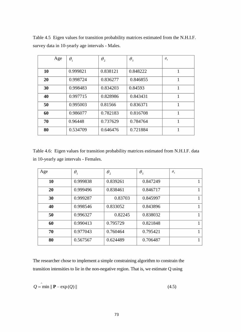
73
Table 4.5 Eigen values for transition probability matrices estimated from the N.H.I.F.
survey data in 10-yearly age intervals - Males.
Age 1 2 3 4
10 0.999821 0.838121 0.848222 1
20 0.998724 0.836277 0.846855 1
30 0.998483 0.834203 0.84593 1
40 0.997715 0.828986 0.843431 1
50 0.995003 0.81566 0.836371 1
60 0.986077 0.782183 0.816708 1
70 0.96448 0.737629 0.784764 1
80 0.534709 0.646476 0.721884 1
Table 4.6: Eigen values for transition probability matrices estimated from N.H.I.F. data
in 10-yearly age intervals - Females.
Age 1 2 3 4
10 0.999838 0.839261 0.847249 1
20 0.999496 0.838461 0.846717 1
30 0.999287 0.83703 0.845997 1
40 0.998546 0.833052 0.843896 1
50 0.996327 0.82245 0.838032 1
60 0.990413 0.795729 0.821848 1
70 0.977043 0.760464 0.795421 1
80 0.567567 0.624489 0.706487 1
The researcher chose to implement a simple constraining algorithm to constrain the
transition intensities to lie in the non-negative region. That is, we estimate Q using
minQ || P – exp )(Q || (4.5)
74
such that the elements ( i ~ j) of Q are non – negative.
The procedure incorporates a least squares routine, using the unconstrained transition
intensities as starting values and exp (Q) evaluated using a Taylor series expansion used by
Moler and Van Loan (1978) for series computations of matrix exponentials, thus:
Exp(Q) = ........!
1......
!2
11
!
1 2
0
n
n
n Qn
QQQn
Tables 4.7 and 4.8 show the annual constrained transition intensities calculated using the
above algorithm at 10-yearly age intervals for both males and females respectively.
Interestingly, the constraining procedure results in Q having the non-negative off diagonal
entries estimated as zero and recovery transitions only occurring progressively by one state
- a likely feature of estimating transition intensities from transition probabilities estimated
using Rickayzen and Walsh's (2002) framework.
Figures 4.4 and 4.5 illustrate the constrained transition intensities for both males and
females from the healthy/able state estimated using the simple constraining algorithm
described above.
Several important observations may be made here among them the fact that Qs no
longer contains any negative `transition intensities'. Secondly, the constraining
procedure does not impact on the unconstrained negative intensities in isolation. All
elements of the transition intensity matrix will be affected. However, a comparison of
the unconstrained transition intensities against the resulting constrained transition
intensities for both males and females reveals only marginal differences to other
elements as a result of the constraining procedure.
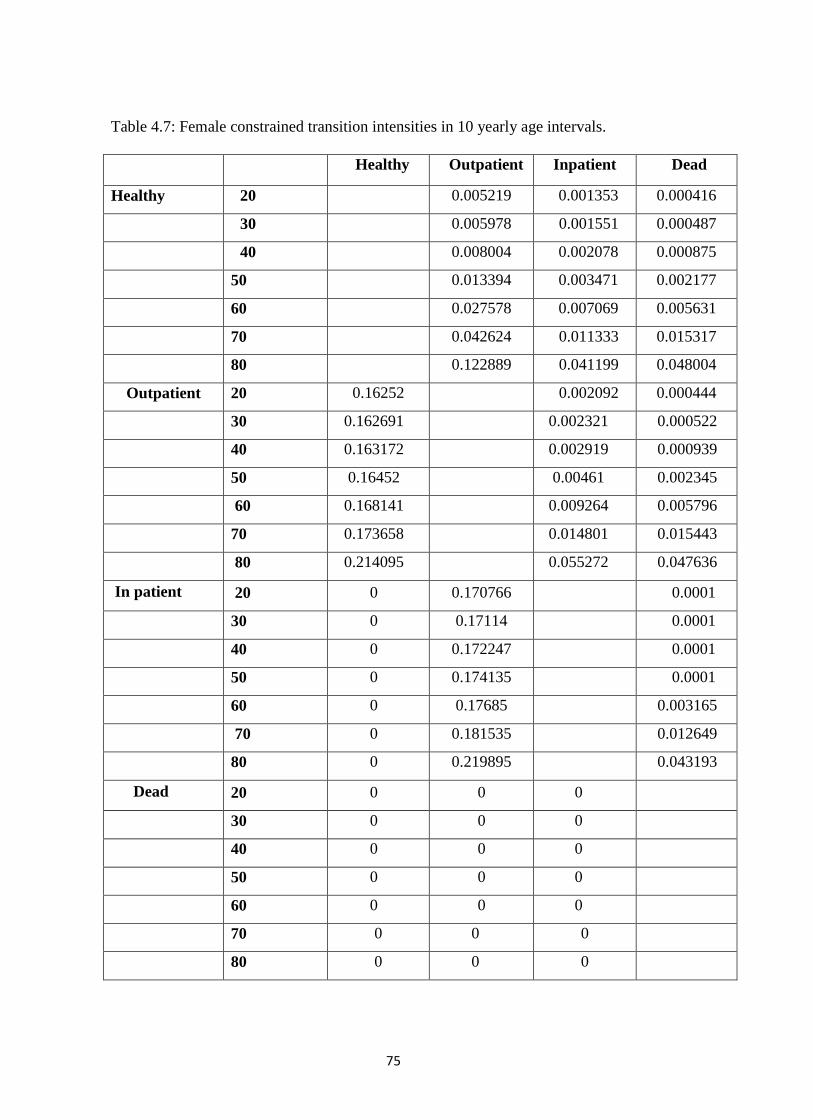
75
Table 4.7: Female constrained transition intensities in 10 yearly age intervals.
Healthy Outpatient Inpatient Dead
Healthy 20 0.005219 0.001353 0.000416
30 0.005978 0.001551 0.000487
40 0.008004 0.002078 0.000875
50 0.013394 0.003471 0.002177
60 0.027578 0.007069 0.005631
70 0.042624 0.011333 0.015317
80 0.122889 0.041199 0.048004
Outpatient 20 0.16252 0.002092 0.000444
30 0.162691 0.002321 0.000522
40 0.163172 0.002919 0.000939
50 0.16452 0.00461 0.002345
60 0.168141 0.009264 0.005796
70 0.173658 0.014801 0.015443
80 0.214095 0.055272 0.047636
In patient 20 0 0.170766 0.0001
30 0 0.17114 0.0001
40 0 0.172247 0.0001
50 0 0.174135 0.0001
60 0 0.17685 0.003165
70 0 0.181535 0.012649
80 0 0.219895 0.043193
Dead 20 0 0 0
30 0 0 0
40 0 0 0
50 0 0 0
60 0 0 0
70 0 0 0
80 0 0 0
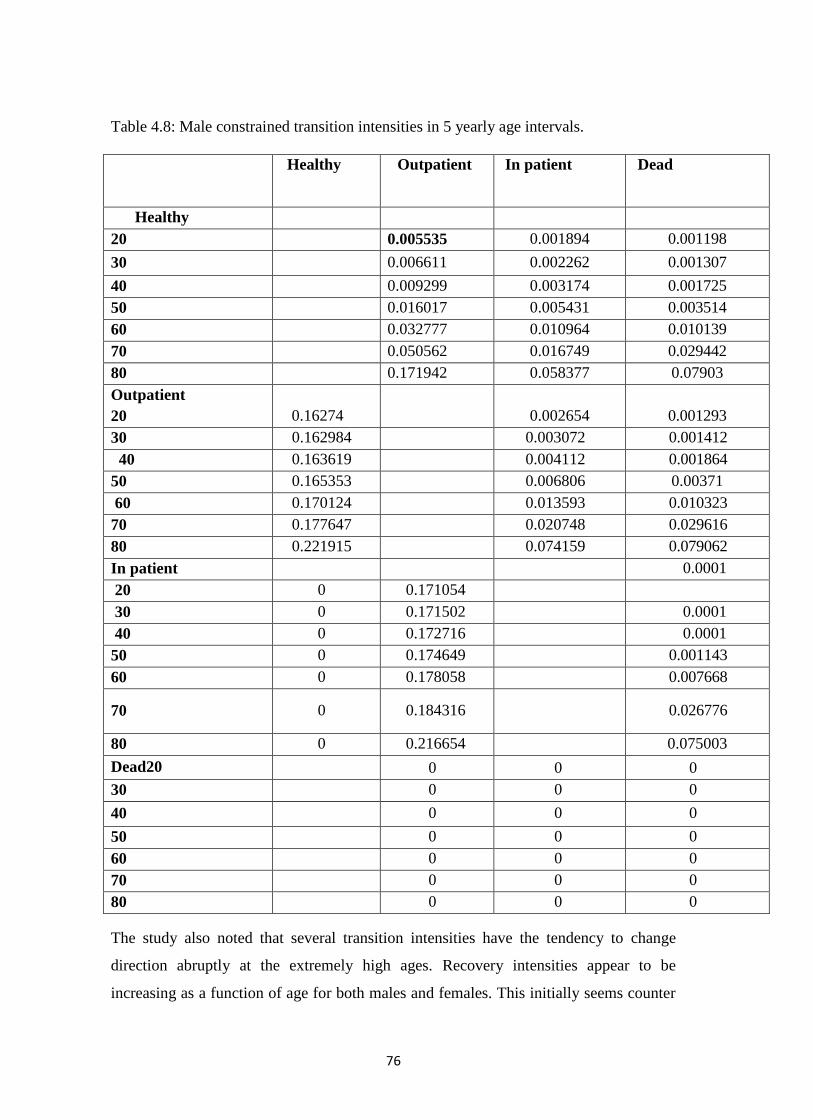
76
Table 4.8: Male constrained transition intensities in 5 yearly age intervals.
Healthy Outpatient In patient Dead
Healthy
20 0.005535 0.001894 0.001198
30 0.006611 0.002262 0.001307
40 0.009299 0.003174 0.001725
50 0.016017 0.005431 0.003514
60 0.032777 0.010964 0.010139
70 0.050562 0.016749 0.029442
80 0.171942 0.058377 0.07903
Outpatient
20 0.16274
0.002654 0.001293
30 0.162984 0.003072 0.001412
40 0.163619 0.004112 0.001864
50 0.165353 0.006806 0.00371
60 0.170124 0.013593 0.010323
70 0.177647 0.020748 0.029616
80 0.221915 0.074159 0.079062
In patient 0.0001
20 0 0.171054
30 0 0.171502 0.0001
40 0 0.172716 0.0001
50 0 0.174649 0.001143
60 0 0.178058 0.007668
70 0 0.184316 0.026776
80 0 0.216654 0.075003
Dead20 0 0 0
30 0 0 0
40 0 0 0
50 0 0 0
60 0 0 0
70 0 0 0
80 0 0 0
The study also noted that several transition intensities have the tendency to change
direction abruptly at the extremely high ages. Recovery intensities appear to be
increasing as a function of age for both males and females. This initially seems counter
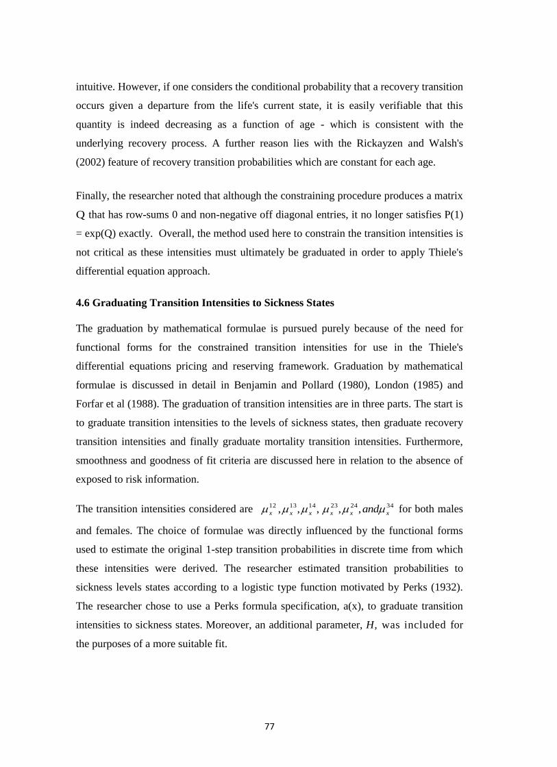
77
intuitive. However, if one considers the conditional probability that a recovery transition
occurs given a departure from the life's current state, it is easily verifiable that this
quantity is indeed decreasing as a function of age - which is consistent with the
underlying recovery process. A further reason lies with the Rickayzen and Walsh's
(2002) feature of recovery transition probabilities which are constant for each age.
Finally, the researcher noted that although the constraining procedure produces a matrix
Q that has row-sums 0 and non-negative off diagonal entries, it no longer satisfies P(1)
= exp(Q) exactly. Overall, the method used here to constrain the transition intensities is
not critical as these intensities must ultimately be graduated in order to apply Thiele's
differential equation approach.
4.6 Graduating Transition Intensities to Sickness States
The graduation by mathematical formulae is pursued purely because of the need for
functional forms for the constrained transition intensities for use in the Thiele's
differential equations pricing and reserving framework. Graduation by mathematical
formulae is discussed in detail in Benjamin and Pollard (1980), London (1985) and
Forfar et al (1988). The graduation of transition intensities are in three parts. The start is
to graduate transition intensities to the levels of sickness states, then graduate recovery
transition intensities and finally graduate mortality transition intensities. Furthermore,
smoothness and goodness of fit criteria are discussed here in relation to the absence of
exposed to risk information.
The transition intensities considered are 342423141312 ,,,,, xxxxxx and for both males
and females. The choice of formulae was directly influenced by the functional forms
used to estimate the original 1-step transition probabilities in discrete time from which
these intensities were derived. The researcher estimated transition probabilities to
sickness levels states according to a logistic type function motivated by Perks (1932).
The researcher chose to use a Perks formula specification, a(x), to graduate transition
intensities to sickness states. Moreover, an additional parameter, H, was included for
the purposes of a more suitable fit.
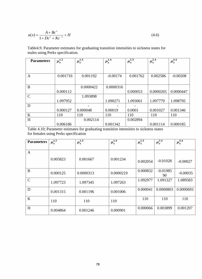
78
HKcDc
BcAxa
xx
x
1)( (4.6)
Table4.9. Parameter estimates for graduating transition intensities to sickness states for
males using Perks specification.
Parameters
A 0.001716 0.001192
-0.00174
0.001762 0.002586 -0.00208
B
0.000112
0.0000422
0.0000316
0.000053
0.0000265
0.0000447
C
1.097952
1.093898
1.090271
1.093061
1.097779
1.098795
D
0.000127
-
0.000048
-
0.00019
-
0.0001
0.001027
0.001346
K 110 110 110 110 110 110
H
0.006186
0.002114
0.001342
0.002894
0.001114
0.000185
Table 4.10; Parameter estimates for graduating transition intensities to sickness states
for females using Perks specification
Parameters
A
0.005823 0.001667 0.001234
0.002054
-0.01028
-0.00027
B 0.000125 0.0000313 0.0000219
0.000832
-0.01985
90 -0.00035
C 1.097723 1.097345 1.097263
1.092977
1.091327
1.089583
D 0.001315 0.001196 0.001006
0.000041
0.0000803
0.0000693
K 110 110 110
110
110
110
H 0.004864 0.001246 0.000901
0.000066 0.003899
0.001207
79
4.7 Graduating Recovery Transitions
The transition intensities considered here are those concerning recovery p32, psi and
1 u . Graduations using the Gompertz- Makeham and Logit Gompertz-Makeham
formula of type (r,s) have been investigated previously using health and disability
related data ( CMIR 6 (1983) and CMIR 17 (1991)). Generally, the Logit Gompertz-
Makeham formula is expressed as:
)(1
)()(
5,
5,
5,
xGM
xGMxLGM
r
r
r
Where
r
i
r
ri
ri
i
i
i
r xxxGM1
5
1
115, exp)(
(4.7)
is the Gompertz- Makeham formula of type (r,s) (Forfar et al 1985).
A LogitGompertz-Makeham formula, LG M ( 1 , 2 ) , was found to fit sufficiently well
here for recovery intensities, that is:
)exp(1
)exp(
321
3210
x
xji
x
(4.8)
Female recovery transition intensities had the tendency to change direction abruptly at
extremely high ages. Note, however, that male recovery transition intensities did not
have this problem. The researcher chose to extrapolate over the higher ages for the
female graduations. This was chosen purely to remain consistent with formulae used to
graduate male recovery intensities. In any case, for our ultimate purpose of pricing
calculations, it is anticipated that the impact of this assumption will be minimal.
The parameters },,{ 321 were estimated using unweighted least squares. The
parameter estimates for graduating recovery transition intensities for both males and
females by mathematical formula as specified in equation (4.8) are presented in Tables
4.11 and 4.12 respectively.
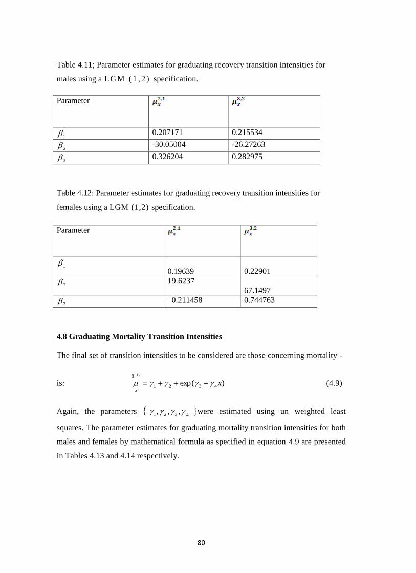
80
Table 4.11; Parameter estimates for graduating recovery transition intensities for
males using a L G M ( 1 , 2 ) specification.
Parameter
1 0.207171 0.215534
2 -30.05004 -26.27263
3 0.326204 0.282975
Table 4.12: Parameter estimates for graduating recovery transition intensities for
females using a LGM (1,2) specification.
Parameter
1
0.19639
0.22901
2 19.6237
67.1497
3 0.211458 0.744763
4.8 Graduating Mortality Transition Intensities
The final set of transition intensities to be considered are those concerning mortality -
is: )exp( 4321
0 6
x
i
x
(4.9)
Again, the parameters 4321 ,,, were estimated using un weighted least
squares. The parameter estimates for graduating mortality transition intensities for both
males and females by mathematical formula as specified in equation 4.9 are presented
in Tables 4.13 and 4.14 respectively.
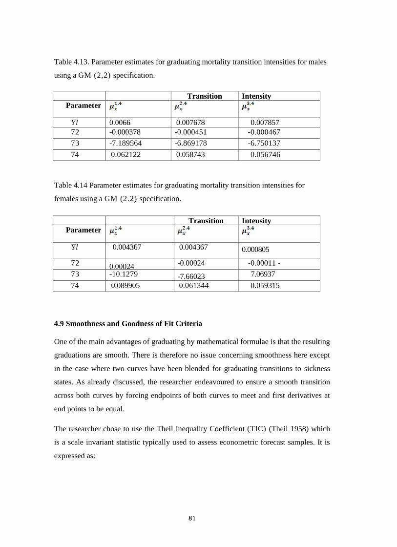
81
Table 4.13. Parameter estimates for graduating mortality transition intensities for males
using a GM (2,2) specification.
Transition Intensity
Parameter
lix
lix
lix
Yl 0.0066 0.007678 0.007857
72 -0.000378 -0.000451 -0.000467
73 -7.189564 -6.869178 -6.750137
74 0.062122 0.058743 0.056746
Table 4.14 Parameter estimates for graduating mortality transition intensities for
females using a GM (2.2) specification.
Transition Intensity
Parameter
lix
lix
lix
Yl 0.004367
-0.000031 -0.00024
-10.1279 -7.66023
0.089905
0.061344
0.004367 0.000805
-0.00011 -7.06937
0.059315
72 0.00024
-10.1279 -7.66023
0.089905
0.061344
-0.00024 -0.00011 -
73 -10.1279 -7.66023
7.06937
74 0.089905 0.061344 0.059315
4.9 Smoothness and Goodness of Fit Criteria
One of the main advantages of graduating by mathematical formulae is that the resulting
graduations are smooth. There is therefore no issue concerning smoothness here except
in the case where two curves have been blended for graduating transitions to sickness
states. As already discussed, the researcher endeavoured to ensure a smooth transition
across both curves by forcing endpoints of both curves to meet and first derivatives at
end points to be equal.
The researcher chose to use the Theil Inequality Coefficient (TIC) (Theil 1958) which
is a scale invariant statistic typically used to assess econometric forecast samples. It is
expressed as:
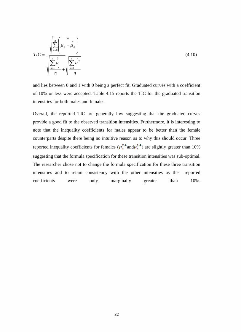
82
nn
TICn
x
n
x x
n
x
xx
1
2
1
0
0
0
2
(4.10)
and lies between 0 and 1 with 0 being a perfect fit. Graduated curves with a coefficient
of 10% or less were accepted. Table 4.15 reports the TIC for the graduated transition
intensities for both males and females.
Overall, the reported TIC are generally low suggesting that the graduated curves
provide a good fit to the observed transition intensities. Furthermore, it is interesting to
note that the inequality coefficients for males appear to be better than the female
counterparts despite there being no intuitive reason as to why this should occur. Three
reported inequality coefficients for females ( and ) are slightly greater than 10%
suggesting that the formula specification for these transition intensities was sub-optimal.
The researcher chose not to change the formula specification for these three transition
intensities and to retain consistency with the other intensities as the reported
coefficients were only marginally greater than 10%.
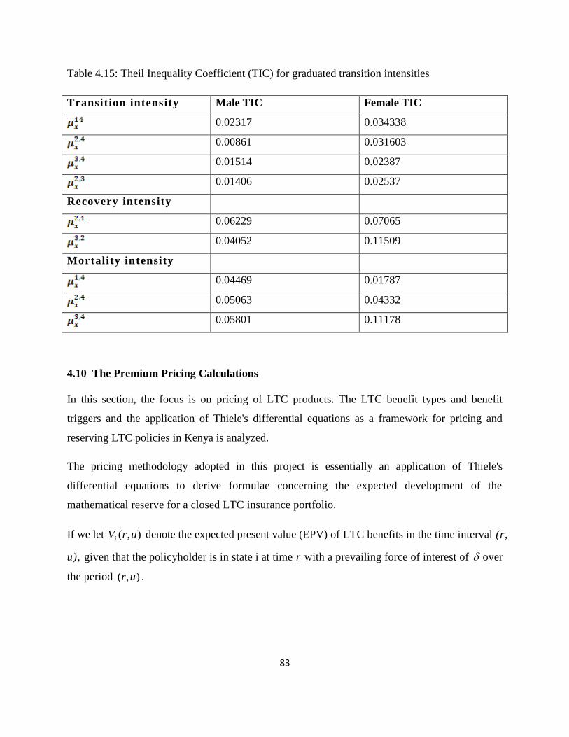
83
Table 4.15: Theil Inequality Coefficient (TIC) for graduated transition intensities
Transition intensity Male TIC Female TIC
0.02317 0.034338
0.00861 0.031603
0.01514 0.02387
0.01406 0.02537
Recovery intensity
0.06229 0.07065
0.04052 0.11509
Mortality intensity
0.04469 0.01787
0.05063 0.04332
0.05801 0.11178
4.10 The Premium Pricing Calculations
In this section, the focus is on pricing of LTC products. The LTC benefit types and benefit
triggers and the application of Thiele's differential equations as a framework for pricing and
reserving LTC policies in Kenya is analyzed.
The pricing methodology adopted in this project is essentially an application of Thiele's
differential equations to derive formulae concerning the expected development of the
mathematical reserve for a closed LTC insurance portfolio.
If we let ),( urVi denote the expected present value (EPV) of LTC benefits in the time interval (r,
u), given that the policyholder is in state i at time r with a prevailing force of interest of over
the period ),( ur .
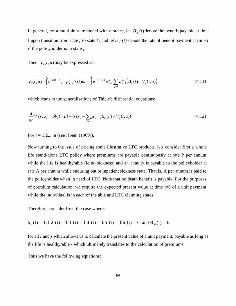
84
In general, for a multiple state model with n states, let )(tB jk denote the benefit payable at time
t upon transition from state j to state k, and let b j (t) denote the rate of benefit payment at time t
if the policyholder is in state j.
Then, ),( urVi may be expressed as:
u
r ij
jij
ij
x
ii
rx
rt
i
ii
rxrt
u
r
rt
i utVtBpedttbpeurV ),()()(),( 1
)()( (4.11)
which leads to the generalisations of Thiele's differential equations:
)),()(()(),(),(
ij
jij
ij
rxiii utVrBrburVurVdr
d (4.12)
For i = 1,2,...,n (see Hoem (1969)).
Now turning to the issue of pricing some illustrative LTC products, lets consider first a whole
life stand-alone LTC policy where premiums are payable continuously at rate P per annum
while the life is healthy/able (ie no sickness) and an annuity is payable to the policyholder at
rate A per annum while enduring out or inpatient sickness state. That is, A per annum is paid to
the policyholder when in need of LTC. Note that no death benefit is payable. For the purposes
of premium calculation, we require the expected present value at time t=0 of a unit payment
while the individual is in each of the able and LTC claiming states.
Therefore, consider first, the case where:
b, (t) = 1, b2 (t) = b3 (t) = b4 (t) = b5 (t) = b6 (t) = 0, and B ij (t) = 0
for all i and j which allows us to calculate the present value of a unit payment, payable as long as
the life is healthy/able - which ultimately translates to the calculation of premiums.
Thus we have the following equations:
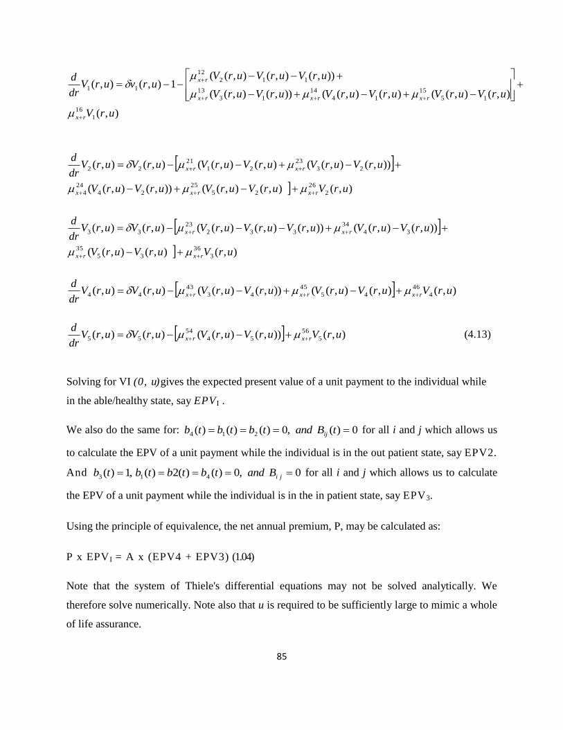
85
),(
),(),((),(),(()),(),((
)),(),(),((1),(),(
1
16
15
15
14
14
13
13
112
12
11
urV
urVurVurVurVurVurV
urVurVurVurvurV
dr
d
rx
rxrxrx
rx
),(),(),(()),(),((
)),(),((),(),((),(),(
2
26
25
25
24
24
4
23
23
21
21
22
urVurVurVurVurV
urVurVurVurVurVurVdr
d
rxrxx
rxrx
),(),(),((
)),(),(()),(),(),((),(),(
3
36
35
35
34
34
332
23
33
urVurVurV
urVurVurVurVurVurVurVdr
d
rxrx
rxrx
),(),(),(()),(),((),(),( 4
46
45
45
43
43
44 urVurVurVurVurVurVurVdr
drxrxrx
),()),(),((),(),( 5
56
54
54
55 urVurVurVurVurVdr
drxrx (4.13)
Solving for VI (0, u) gives the expected present value of a unit payment to the individual while
in the able/healthy state, say EPV I .
We also do the same for: 0)(,0)()()( 214 tBandtbtbtb ij for all i and j which allows us
to calculate the EPV of a unit payment while the individual is in the out patient state, say EPV2.
And 0,0)()(2)(,1)( 413 jiBandtbtbtbtb for all i and j which allows us to calculate
the EPV of a unit payment while the individual is in the in patient state, say EPV3.
Using the principle of equivalence, the net annual premium, P, may be calculated as:
P x EPV I = A x (EPV4 + EPV3) (1.04)
Note that the system of Thiele's differential equations may not be solved analytically. We
therefore solve numerically. Note also that u is required to be sufficiently large to mimic a whole
of life assurance.
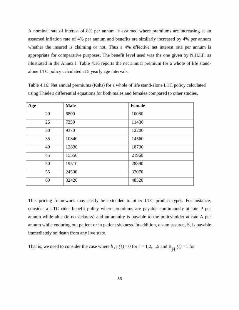
86
A nominal rate of interest of 8% per annum is assumed where premiums are increasing at an
assumed inflation rate of 4% per annum and benefits are similarly increased by 4% per annum
whether the insured is claiming or not. Thus a 4% effective net interest rate per annum is
appropriate for comparative purposes. The benefit level used was the one given by N.H.I.F. as
illustrated in the Annex I. Table 4.16 reports the net annual premium for a whole of life stand-
alone LTC policy calculated at 5 yearly age intervals.
Table 4.16: Net annual premiums (Kshs) for a whole of life stand-alone LTC policy calculated
using Thiele's differential equations for both males and females compared to other studies.
Age Male Female
20 6800 10080
25 7250 11430
30 9370 12200
35 10840 14560
40 12830 18730
45 15550 21960
50 19510 28890
55 24590 37070
60 32420 48520
This pricing framework may easily be extended to other LTC product types. For instance,
consider a LTC rider benefit policy where premiums are payable continuously at rate P per
annum while able (ie no sickness) and an annuity is payable to the policyholder at rate A per
annum while enduring out patient or in patient sickness. In addition, a sum assured, S, is payable
immediately on death from any live state.
That is, we need to consider the case where b 1 ; (t )= 0 for i = 1,2,...,5 and Bj4
(t) =1 for
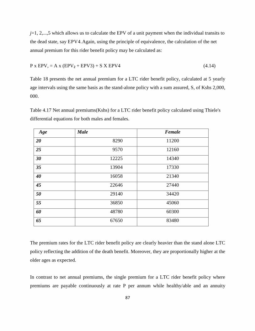
87
j=1, 2,...,5 which allows us to calculate the EPV of a unit payment when the individual transits to
the dead state, say EPV4.Again, using the principle of equivalence, the calculation of the net
annual premium for this rider benefit policy may be calculated as:
P x EPV, = A x (EPV2 + EPV3) + S X EPV4 (4.14)
Table 18 presents the net annual premium for a LTC rider benefit policy, calculated at 5 yearly
age intervals using the same basis as the stand-alone policy with a sum assured, S, of Kshs 2,000,
000.
Table 4.17 Net annual premiums(Kshs) for a LTC rider benefit policy calculated using Thiele's
differential equations for both males and females.
Age Male Female
20 8290 11200
25 9570 12160
30 12225 14340
35 13904 17330
40 16058 21340
45 22646 27440
50 29140 34420
55 36850 45060
60 48780 60300
65 67650 83480
The premium rates for the LTC rider benefit policy are clearly heavier than the stand alone LTC
policy reflecting the addition of the death benefit. Moreover, they are proportionally higher at the
older ages as expected.
In contrast to net annual premiums, the single premium for a LTC rider benefit policy where
premiums are payable continuously at rate P per annum while healthy/able and an annuity
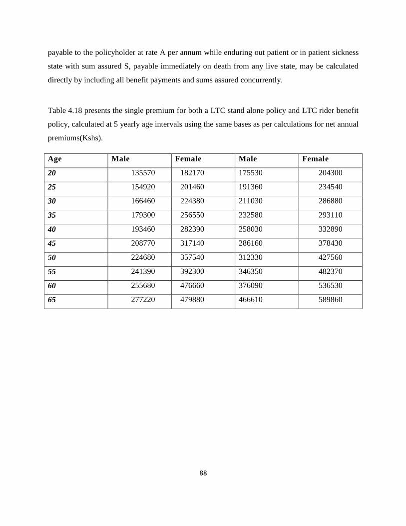
88
payable to the policyholder at rate A per annum while enduring out patient or in patient sickness
state with sum assured S, payable immediately on death from any live state, may be calculated
directly by including all benefit payments and sums assured concurrently.
Table 4.18 presents the single premium for both a LTC stand alone policy and LTC rider benefit
policy, calculated at 5 yearly age intervals using the same bases as per calculations for net annual
premiums(Kshs).
Age Male Female Male Female
20 135570 182170 175530 204300
25 154920 201460 191360 234540
30 166460 224380 211030 286880
35 179300 256550 232580 293110
40 193460 282390 258030 332890
45 208770 317140 286160 378430
50 224680 357540 312330 427560
55 241390 392300 346350 482370
60 255680 476660 376090 536530
65 277220 479880 466610 589860

89
4.11 Reserving for illustrative LTC products
Having solved for the net annual premium, P, we may calculate the development of the reserve
for each state - All we need to specify are the
boundary conditions given as:
(4.15)
For illustrative purposes, we present results for the reserve profile for an LTC stand-alone policy
at different states in figure 4.1 .
Overall, the results in Figure 4.1 show that the behavior of is largely as expected.
Reserves for non-LTC claiming states begin at zero and gradually build
before falling and ultimately releasing the entire reserve at the end of the policy term. Reserves
in LTC claiming states, however, begin at very high levels and gradually fall to zero at the end of
the policy term.
Insurers are likely to be most concerned with as the vast majority of LTC policies would
ordinarily be affected while the individual is in the healthy state . In each of the reserve profiles
calculated here, has a zero reserve at both contract issue and termination which is
directly attributable to the equivalence principle. An interesting point to note is that the reserve
levels for both the outpatient and inpatient states and begin at a positive non-
zero level.
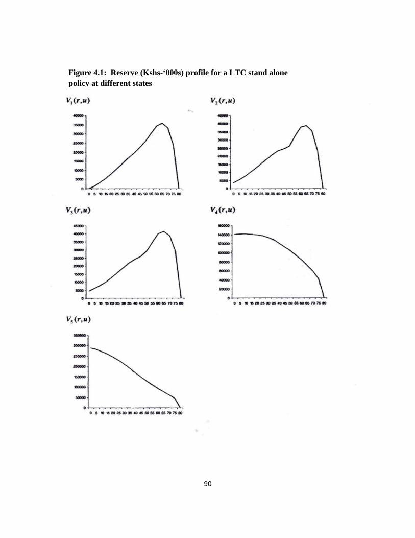
90
Figure 4.1: Reserve (Kshs-‘000s) profile for a LTC stand alone
policy at different states

91
CHAPTER FIVE
SUMMARY, CONCLUSIONS AND RECOMMENDATIONS
5.1 Introduction
This chapter summarizes the study findings according to the research objectives. Conclusions of
major study results are then outlined. Finally, recommendations based on the study findings are
made to the N.H.I.F. Board, the Insurance Regulatory Authority (I.R.A), The Ministry of Health
and actuarial scientists and practitioners on the pricing of Long Term Care Products offered by
the national LTC insurer.
5.2 Summary of the Study Findings
The study used the four state multi state modeling framework to calculate transition intensities
and probabilities of N.H.I.F. members transitioning from the healthy through to out and in
patient sickness states up to death.
The forces of transition, recovery and mortality were estimated using the maximum likelihood
approach with the crude estimates of the same being graduated using parametric methodologies
of Compertz-Mekahem with their logarithmic modifications using logistic variations and Perks
formula.
The membership data sample was categorized according to gender with all the calculations and
estimates of transition intensities, probabilities, graduations, and pricing being based on ea ch
gender.
The study analysis was able to price the net and single premiums for whole life stand alone
and LTC rider benefit policies.
In doing this, a nominal rate of interest of 8% per annum was assumed where premiums were
increasing at an assumed inflation rate of 4% per annum and benefits similarly increased by 4%
per annum whether the insured was claiming or not. Thus a 4% effective net interest rate per
annum was appropriate for comparative purposes.
The study found that transition intensities or forces of transition and probabilities for both males
and females generally behaved as expected with transition probabilities to sickness states
92
increasing with age. Transition through sickness/disability levels was reasonably progressive.
That is, given that a transition out of the sickness/disabled state occurs, there was a higher
probability of moving to a lower sickness/disability level than directly to a more severe
sickness/disability level. At higher ages, however, transition to the in patient sickness exceeding
outpatient sickness/disability levels. This seems reasonable owing to the effects of ageing and
chronic frailty.
Secondly, transition probabilities out of the sick/disabled state appear higher for males than
females. Transition out of the healthy/able state to outpatient and inpatient sickness states
appears higher for females than males. Again, mortality in the inpatient sickness state is higher
for males than females.
These last two points above are particularly interesting as they form the basis of an a priori
expectation that the likelihood of LTC utilization by females will be higher than by males in the
Kenyan population, therefore resulting in more expensive premiums for females.
On the reserving calculations, the study findings revealed that the reserve behavior is largely as expected.
Reserves for non-LTC claiming states begin at zero and gradually build before falling and ultimately
releasing the entire reserve at the end of the policy term.
The study found that for LTC claiming states of outpatient and inpatient the reserves begin at a positive
non zero level since the premiums are not required to be paid by the insured during these states.
5.3 Conclusions
Based on the study findings, the research concludes that the male premium rates are uniformly
less than female premium rates. Again, the transition intensities or forces of transition and
probabilities for both males and females generally behaved as expected with transition
probabilities to sickness states increasing with age.
Transition through sickness/disability levels was reasonably progressive because of treatment so
that there was a higher probability of moving to a lower sickness/disability level than directly to in
patient sickness/disability level. At higher ages, however, transition to the inpatient sickness
93
exceeded the out patient sickness/disability levels. This seems reasonable owing to the effects of
ageing and chronic frailty.
Secondly, transition probabilities out of the sick/disabled state appear higher for males than
females. Transition out of the healthy/able state to outpatient and inpatient sickness states appears
higher for females than males. Again, mortality in the in-patient sickness state is higher for males
than females.
The two observations made form the basis of an a priori expectation that the likelihood of LTC
utilization by females will be higher than by males in the Kenyan population, therefore resulting
in more expensive premiums for females. Although the study did not investigate the nature of
sicknesses for both in and out patient hospital attendances, the conclusion that female utilization
of the medical insurance facility could be attributed to other visits such as prenatal, maternity and
postnatal medical care.
Overall, the study concluded that the net annual premium rates for both males and females
calculated using Thiele's differential equations within a multiple state model framework appear
both reasonable and consistent with past LTC studies with higher rates expected at higher ages.
The study concluded that the reserves for the non LTC claiming state begin at zero and gradually build
up and ultimately releases the entire reserve at the end of the policy term.
The study concludes that for LTC claiming states of outpatient and inpatient, the reserves begin at a
positive non zero level since the premiums are not required to be paid by the insured during these states.
5.4 Recommendations
The non-existence of adequate data in Kenya has been, and will be, a significant obstacle in the introduction
of private LTC insurance in Kenya. It is possible, however, to develop a model for pricing LTC insurance
using the currently available data in Kenya. This can be done via the application of Thiele's differential
equations for a multiple state model. This model, despite its complexity, offers a significant degree of
modeling flexibility and robustness which makes it preferable to traditional annuity inception approaches.

94
This study, to the researcher’s knowledge, represents the first stochastic model developed for the purposes
of pricing reserving LTC in Kenya.
The researcher therefore recommends this pricing and reserving model for the development and design of
the LTC products in the Kenyan insurance industry.
There are, however, a number of limitations here, largely a result of inadequate data. In particular, the
researcher acknowledges the inconsistency of a continuous time Markov chain with the discrete state
model framework. The focus to a great extent in this project has been the development of a model which,
when adequate data becomes available, will produce increasingly accurate results.
The study recommends that a comparative study using both the multi state and multiple decrement
approaches be done in order to arrive at more accurate results in the pricing and reserving of LTC products
in the Kenyan insurance industry.
The study recommended that reserves for non LTC claiming states begin at zero and gradually build up
and ultimately release the entire reserve at the end of the policy term.
For LTC claiming states of outpatient and inpatient, the study recommends that reserves begin at a
positive non zero level since the premiums are not required to be paid by the insured during these states.
5.5 Room for Further Research
Once appropriate LTC specific data become available for Kenya, the following extensions to this study
could be undertaken: One is to allow for all possible modes of recovery in the multiple state model;
secondly, other scholars and actuarial scientists could allow for lapses in the multiple state model.
It is possible to allow for duration in the multiple state models by implementing a semi-Markov
assumption as opposed to a Markov assumption. That is, allow transition intensities to depend on both age
and the duration of stay in the current state.
For comparative purposes, the technical actuarial bases used to price several illustrative LTC products
come from a survey of earlier relevant literature. The model bases here, however, may be easily modified
at the insurer's discretion in another scholarly research.
95
REFERENCES
Alegre, A., Pociello, E., Pons, M., Sarrasi, J., Varea, J. and Vicente, A., 2002, `Actuarial
valuation of long-term care annuities', Paper presented to 6th Insurance: Mathematics and
Economics Congress, Lisbon.
Andrei Kolmogorov, "On Analytical Methods in the Theory of Probability", 448-451, (1931)
Beekman, J. A., 1989 `An alternative premium calculation method for certain long term care
coverage', Actuarial Research Clearing House (ARCH), Vol. H.
Cheng, S.H, Higham, N.J, Kenney, C.S and Laub, A.J, 2001 `Approximating the logarithm of a
matrix to specified accuracy', Society for Industrial and Applied Mathemtics Journal: Matrix
Anal. Appl., Vol 22, No.4, 1112-1125.
CMIR 6, 1983, `Graduation of the mortality experience of female assured lives 1975-78', CMI
Committee.
CMIR 7, 1984, `Sickness experience 1975-78 for individual PHI policies', CMI Committee.
CMIR 17, 1991, `The analysis of permanent health insurance data, CMI Committee
Cordeiro, I. M. F., 2001, `Transition intensities for a model for permanent health insurance',
Documento de Trabalho No 4-2001, Centro de MatematicaAplicada a Previsao e
DecisaoEconomica, Lisbon.
Cowley, A., 1992, Long-Term Care Insurance: International Perspective and Actuarial
Considerations, Publications of the Cologne Re, Number 22.
Cox, D.R a Table 4. 4: Female unconstrained transition intensities calculated from 1-step transition
probabilities in 10 yearly age intervals.
Dickson D.C., Hardy M.R., Waters H.R., (2009), Actuarial Mathematics for Life Contingent
Risks, Cambridge University Press
Miller, H.D, 1965, The Theory of Stochastic Processes, Chapman and Hall, London.
96
Czado, C. and Rudolph, F., 2002, `Application of survival analysis methods to long-term care
insurance', Insurance: Mathematics and Economics, 31, 395-413.
Davies, P.I, and Higham, N.J, 2002, `A Schur-Parlett algorithm for computing matrix functions'
Numerical Analysis Report 404, Manchester Centre for Computational Mathematics.
Davis, E., Beer, J., Cligora, C. and Thorn, A., 2001, `Accounting for change in disability and
severe restriction, 1981-1998', Working papers in social and labour statistics, ABS Working
Paper No. 2W1/1, Canberra.
Eagles, L. M, 1992, `Some problems in pricing long term care contracts', Transactions of the
24`h
International Congress of Actuaries, Montreal, Vol 4, 421-427.
Gatenby, P., 1991, `Long term care', Paper presented to the Staple Inn Actuarial Society.
Gatenby, P. and Ward, N., 1994 `Multiple state modeling', Paper presented to the Staple Inn
Actuarial Society.
Golub, G.H and Van Loan, C.F, 1983, Matrix Computations, Johns Hopkins University Press,
Baltimore, MD.
Haberman, S., 1993, `HIV, AIDS, Markov Chains and PHI', Actuarial Research Paper No.52,
Department of Actuarial Science & Statistics, City University, London.
Haberman, S. and Pitacco, E., 1999, Actuarial Models for Disability Insurance, Chapman &
Ha1UCRC Press, Boca Ratan, R.
Higham, N.J, `Evaluating pade approximants of the matrix logarithm', Society for Industrial and
Applied Mathematics Journal: Matrix Anal. Appl., Vol 22, No.4, 1126-1135.
Hcem, J. M., 1969 Markov chain models in life insurance', Blaster der DeutschenGesellschaft
fur Versicherungsmathematik9, 91-107.
Hcem, J.M., 1988, `The versatility of the Markov chain as a tool in the mathematics of life
insurance', Transactions of the 23'dInternational Congress of Actuaries, Helsinki, 171-202.
97
Israel, R.B, Rosenthal, J.S and Wei, J.Z, 2001, `Finding generators for markov chains via
empirical transition matrices, with applications to credit ratings', Mathematical Finance, Vol.11,
No.2, 245-265.
Janssen, H. K. (1976). "On a Lagrangean for Classical Field Dynamics and Renormalization
Group Calculation of Dynamical Critical Properties". Z. PhysikB23 (4): 377–380.
doi:10.1007/BF01316547.
Jones, B.L, 1992a, `An analysis of long-term care data from Hamilton-Wentworth Ontario',
Actuarial Research Clearing House, Vol 1, 337-352.
Jones, B.L, 1992b, Stochastic Models for Long-Term Care, Ph.D Thesis, University of Waterloo,
Canada.
Jones, B. L, 1993 `Modelling multi-state processes using a Markov assumption', Actuarial
Research Clearing House, Vo1.1, 239-248.
Kulkarni, V.G, 1995, Modeling and Analysis of Stochastic Systems, Chapman and Hall, London.
Leung, E., 2004, `Projecting the needs and costs of long term care in Australia', Australian
Actuarial Journal, Vol. 10, No.2, 301-342.
Levikson, B. and Mizrahi, G., 1994, `Pricing long term care insurance contracts', Insurance:
Mathematics & Economics, 14, 1-18.
Linnemann, P., 1993, `On the application of Thiele's differential equation in life insurance',
Insurance: Mathematics and Economics, 13, 63-74.
London, D., 1985, Graduation: The Revision of Estimates, ACTEX Publishing, Winsted,
Connecticut.
Madden, R. and Wen, X., 2001, `The cost of health as you age: Is it a health hazard?', Australian
Institute of Health and Welfare', Paper presented to Institute of Actuaries of Australia, Sydney.

98
Manton, K.G., 1988, `A longitudinal study of functional change and mortality in the United
States', Journal of Gerontology: Social Sciences, Vol. 43 No. 5, 153-161.
Meiners, M. R., 1989, Data Requirements for Long-Term Care Insurance, National Center for
Health Services Research and Health Care Technology Assessment, U.S. Department of Health
and Human Services.
Moler, C. and Van Loan, C., 1978, `Nineteen Dubious Ways to Compute the Exponential of a
Matrix', Society for Industrial and Applied Mathematics Review, Vol. 20, No. 4, 801-836.
N. N. Bogolyubov (jr) and D. P. Sankovich (1994). "N. N. Bogolyubov and statistical
mechanics". Russian Math. Surveys49(5):
N. N. Bogoliubov and N. M. Krylov (1939). Fokker–Planck equations generated in perturbation
theory by a method based on the spectral properties of a perturbed Hamiltonian.
Norberg, R., 1995, `Differential equations for moments of present values in life insurance',
Insurance: Mathematics & Economics, Vol 17, 1995, 171-180.
Norris, J. R. (1997). "Continuous-time Markov chains I". Markov Chains. p. 60.
doi:10.1017/CBO9780511810633.004. ISBN 9780511810633.
Norris, J. R. (1997). "Discrete-time Markov chains". Markov Chains.
p. 1.:10.1017/CBO9780511810633.003. ISBN 9780511810633.
Norris, J. R. (1997). "Continuous-time Markov chains II". Markov Chains.
p. 108.10.1017/CBO9780511810633.005. ISBN 9780511810633.
Parlett, B.N, 1974, Computation of Functions of Triangular Matrices, Memorandum no. ERL-
M481, Electronics Research Laboratory, College of Engineering, University of California,
Berkeley.
99
Perks, W., 1932, `On some experiments in the graduation of mortality statistics', Journal of the
Institute of Actuaries, Vol. 63, 12-40.
Pitacco, E., 1995, Collective Life Insurance Indexing: A Multistate Approach, International
Congress of Actuaries, Brussels.
Pitacco, E., 1993, `Disability risk models: Towards a unifying approach', Actuarial Research
Paper No.59, Department of Actuarial Science & Statistics, City University, London.
Pritchard, J.D, 2002, The Genetics of Alzheimer's Disease, Modelling Disability and Adverse
Selection in the Long-Term Care Insurance Market, PhD Thesis, Heriot-Watt University,
Scotland.
Reif, L., 1985, `Long-term care. Some lessons from cross-national comparisons', Home Health
Care Services Quarterly, Vol. 5, 329-341.
Renshaw, A. E. and Haberman, S., 1998, ` Modeling the recent time trends in UK permanent
health insurance recovery, mortality and claim inception transition intensities', Actuarial
Research Paper No.113, Department of Actuarial Science & Statistics, City University, London.
Robinson, J., 1996, A Long-Term Care Status Transition Model, The Old-Age Crisis-Actuarial
Opportunities: The Bowles Symposium, 72-79.
Robinson, R., 1992, `Multistate modeling', The Actuary, September, 16-17.
Rickayzen, B. D. and Walsh, D. E. P., 2002, `A multi-state model of disability for the United
Kingdom: Implications for future need for long-term care for the elderly', British Actuarial
Journal, Vol. 8, No. 2: 341-393.
Sansom, R.J. and Waters, H.R., 1988, `Permanent health insurance in the UK: The mathematical
Model and the statistical analysis of the data, Transactions of the International Congress of
Actuaries, Helsinki, Vol 3, 323-339.
100
Service, D. and Pitt, D., 2002, `Disability claims - Does anyone recover?', Australian Actuarial
Journal Vol. 8, 4, 615-639.
Baier, C.; Katoen, J. P.; Hermanns, H. (1999). "Approximative Symbolic Model Checking of
Continuous-Time Markov Chains". CONCUR'99 Concurrency Theory. Lecture Notes in
Computer Science 1664. p. 146. doi:10.1007/3-540-48320-9_12. ISBN 978-3-540-66425-3.
Serfozo, R. F. (1979). "Technical Note--An Equivalence Between Continuous and Discrete Time
Markov Decision Processes". Operations Research27 (3): 616–620. doi:10.1287/opre.27.3.616.
JSTOR 170221. edit
William J. Stewart (1994). Introduction to the Numerical Solution of Markov Chains. Princeton
University Press. pp. 17–23. ISBN 0-691-03699-3.
Baier, C.; Katoen, J. P.; Hermanns, H. (1999). "Approximative Symbolic Model Checking of
Continuous-Time Markov Chains". CONCUR'99 Concurrency Theory. Lecture Notes in
Computer Science 1664. p. 146. doi:10.1007/3-540-48320-9_12. ISBN 978-3-540-66425-3.
Serfozo, R. F. (1979). "Technical Note--An Equivalence Between Continuous and Discrete Time
Markov Decision Processes". Operations Research27 (3): 616–620. doi:10.1287/opre.27.3.616.
JSTOR 170221.
Norris, J. R. (1997). "Continuous-time Markov chains I". Markov Chains. p. 60.
doi:10.1017/CBO9780511810633.004. ISBN 9780511810633.
Norris, J. R. (1997). "Continuous-time Markov chains II". Markov Chains. p. 108.
doi:10.1017/CBO9780511810633.005. ISBN 9780511810633.
Etheridge, A. (2002). A Course in Financial Calculus. Cambridge University Press.
Risken, H., "The Fokker-Planck equation: Methods of solution and applications" 1996, Springer
Leo P. Kadanoff (2000). Statistical Physics: statics, dynamics and renormalization. World
Scientific. ISBN 981-02-3764-2.

101
Scott W.F., (1999). Life Assurance Mathematics, AB24 3UE, University of Aberdeen.
Scott W.F. (1991), Some Statistical Aspects of Mortality Investigations, JIA 118
University of Nairobi, Lecture Notes, Life Insurance Mathematics, by Prof. Richard Simwa,
2012
William J. Stewart (1994). Introduction to the Numerical Solution of Markov Chains. Princeton
University Press. pp. 17–23. ISBN 0-691-03699-3.
Zinn-Justin, Jean (1996). Quantum field theory and critical phenomena. Oxford: Clarendon
Press. ISBN 0-19-851882-X.

102
N.H.I.F.’s MEMBERS’ SERVICES LTC INSURANCE COVER
Characteristics of the cover
1. Employees actively in civil service and disciplined services are eligible for cover
2. Only the principle member, spouse and three (3) children are covered. (Additional
children can be covered at an extra premium as stipulated in annex II)
3. Dependant children are eligible for cover upto 18 years of age. However with proof that
the child is enrolled in full time learning institution, they are covered upto 25 years of
age. Children with disabilities are also covered past 18 years of age.
4. Medical cover commences immediately upon registration and payment of full premium
for new employees. No waiting period is imposed.
5. Annual medical checkup for the member is required for the principal member.
6. Out-patient visits will attract a co-payment of KES 100 and KES 200 in government and
other facilities per visit .
7. Out-patient dental and optical cover available only on referral basis.
8. Out-patient facilities shall be based on choice made by member with an option of
changing after three months except in cases of emergency, travel on duty or transfer. In
order to change outpatient facility, one must fill in a consent form which will be available
online or at the NHIF offices.
How to Register As an NHIF Member
1. Fill in an NHIF 2 Application form (available at any NHIF office & on our website).
Online registration is also acceptable (please see instructions below).
2. Attach colored passport size photos of contributor and all declared dependant(s)
3. Attach photocopies of identification cards for contributor and spouse (If married)
4. Attach copies of birth certificate of child(ren) or birth notification for child(ren) below
six (6) months,adoption certificate where applicable. Also include details of additional
children you may wish to cover in the enhanced scheme and you are willing to pay
additional premiums.
5. Submit duly filled application form to the nearest NHIF office

103
BENEFITS PACKAGE
1. In-patient cover
Under this cover, members will access:
Hospital accommodation charges
Nursing care
Diagnostic, laboratory or other medically necessary facilities and services
Physician’s, surgeon’s, anesthetist’s, or physiotherapist’s fees
Operating theater charges
Specialist consultations or visits
Drugs, dressing and medications prescribed by treating physician for in-hospital use
Day care services such as surgery and other medical services deemed fit by the physician
Pre-hospitalization procedures such as laboratory, x-ray or other medical diagnostic
procedures which results in a member being admitted on the same day the tests are done.
Ambulance services for transportation and transfer of a sick member/dependant to
another facility
2. Out-patient cover
The out-patient cover shall include:
Consultation
Laboratory investigations and X-ray services
Drugs administration and dispensing
Dental health care services
Radiological examinations
Nursing and midwifery services
Minor surgical services
Physiotherapy services
Optical care
Occupational therapy services

104
Referral for specialized services
3. Maternity cover and reproductive health
Consultation and treatment for both mother and child
Normal and caesarian section
Family planning services excluding fertility treatment
4. Dental cover
Dental consultation
Cost of filling
X-rays
Extractions including surgical extractions together with anaesthetics fees, hospital
and operating theatre cost.
The cover does not include:
The cost of replacement or repairs of old dentures, bridges and plates unless
damage arises directly from accidental, external and visible means
Orthodontic treatment of cosmetic nature
5. Optical Cover
Cost of eyeglasses (limited to a pair per family unless proven medically
necessary)
Frames
Eye testing fees
The cover does not include:
The cost of frames replacement unless directly caused by an injury to an eye
Replacement of lenses unless necessitated in course of further treatment
6. Ex-gratia payments
NHIF shall not be liable for Ex-gratia payments upon the limits being exhausted.

105
7. Group life cover
NHIF shall pay death benefit upon the demise of a member
8. Last expense cover
NHIF shall, upon written notification of death of a member while this cover is in force,
pay to the client or such other person or persons as the client may in writing direct, the
amount specified in the Annex I to cater for the funeral expenses.
EXCLUSIONS
1. Expenses incurred by a member as a result of:
Investigations, treatment, surgery for obesity or its sequel, cosmetic or beauty treatment
and /or surgery
Massage unless necessary for treatment i.e following an accident
Stays at sanatoria, old age homes, places of rest etc
Treatment by chiropractors, acupuncturitst and herbalists, stays and /or maintenance or
treatment received in nature cure clinics or similar establishments or private beds
registered within a nursing home, convalescent and /or rest homes
Claim for expenses incurred whilst the member was outside territorial limits of kenya
unless a kenyan who is temporarily abroad and needs emergency treatment for illness
or injury that occurs during the period of travel provided six weeks is not exceeded.
Fertility treatment related to infertility and impotence
Vaccines other than those of KEPH
2. Charges recoverable under any Work Injury Benefits Act or any other medical plan

106
ANNEX I: N.H.I.F.’s LIMITS OF LIABILITY
CIVIL
SERVICE JOB
GROUPS
DISCIPLINED
FORCES
GRADES
STATE LAW
OFFICE
GRADES
IN-PATIENT
LIMIT (KES)
OUT-
PATIENT
LIMIT(KES)
A-G PG,1,2,3 - No Limit No Limit
H PG 4 - No Limit No Limit
J PG 5 - No Limit No Limit
K PG 6 SL 1 No Limit No Limit
L PG 7 SL 2 No Limit No Limit
M PG 8 & 9 SL 3 No Limit No Limit
N PG 10 SL 4 1,130,000 80,000
P PG 11 SL 5 1,250,000 80,000
Q PG 12 SL 6 1,500,000 100,000
R,S,T PG 13,14 SL 7,8,9 2,000,000 150,000
DENTAL & OPTICAL COVER
CIVIL
SERVICE JOB
GROUPS
DISCIPLINED
FORCES
GRADES
STATE LAW
OFFICE
GRADES
DENTAL
COVER
OPTICAL
COVER
A-M PG1-9 SL 1-3 10,000 10,000
N-Q PG 10-12 SL 4-6 20,000 20,000
R-T PG 13-14 SL 7-9 30,000 30,000

107
GROUP LIFE & LAST EXPENSE
CIVIL
SERVICE JOB
GROUPS
DISCIPLINED
FORCES
GRADES
STATE LAW
OFFICE
GRADES
GROUP LIFE
(KES)
LAST
EXPENSE
(KES)
A-G PG,1,2,3 - 200,000 40,000
H PG 4 - 200,000 40,000
J PG 5 - 200,000 50,000
K PG 6 SL 1 250,000 50,000
L PG 7 SL 2 250,000 50,000
M PG 8 & 9 SL 3 300,000 60,000
N PG 10 SL 4 300,000 70,000
P PG 11 SL 5 350,000 80,000
Q PG 12 SL 6 400,000 80,000
R,S,T PG 13,14 SL 7,8,9 500,000 100,000

108
ANNEX II: N.H.I.F.’s ADDITIONAL DEPENDANT(S)
Additional dependant(s’) premium for in-patient and out-patient limits within the unit per annum
JOB GROUP PREMIUM OF EACH
ADDITIONAL DEPENDANT
(ONE) (KES)
OPTION 1
PREMIUM OF UNLIMITED
ADDITIONAL DEPENDANT(S)
(KES)
OPTION 2
A-G,PG,1,2,3 3,500 6,000
H,PG 4 3,500 6,000
J, PG 5 3,500 6,000
K, PG 6, SL 1 3,500 6,000
L, PG 7,SL 2 3,500 6,000
M, PG 8,9,SL 3 3,500 6,000
N, PG 10,SL 4 6,000 12,000
P, PG 11,SL 5 6,000 12,000
Q, PG 12,SL 6 6,000 12,000
R,S,T,PG 13,14
& SL 7,8,9
9,000 20,000