An advanced visualization system An advanced visualization system for planetary dynamo simulationsfor planetary dynamo simulations

Moritz Heimpel1, Pierre Boulanger2, Curtis Badke1, Farook Al-Shamali1, Jonathan Aurnou3

1 Institute for Geophysical Research, Department of Physics, University of Alberta

2 Department of Computing Sciences, University of Alberta

3 Department of Earth and Space Sciences, University of California, Los Angeles

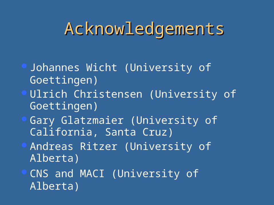
AcknowledgementsAcknowledgements

Johannes Wicht (University of Goettingen)Ulrich Christensen (University of

Goettingen)Gary Glatzmaier (University of California,

Santa Cruz) Andreas Ritzer (University of Alberta)CNS and MACI (University of Alberta)

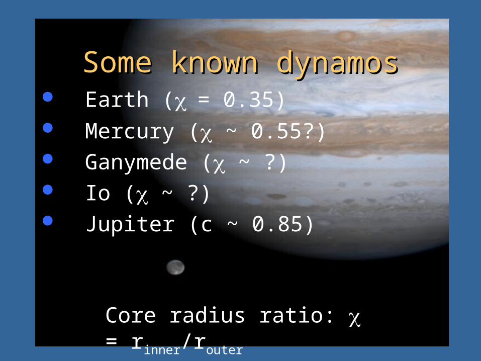
Some known dynamosSome known dynamos Earth (= 0.35) Mercury ( ~ 0.55?) Ganymede ( ~ ?) Io ( ~ ?) Jupiter (c ~ 0.85)

Core radius ratio: = rinner/router

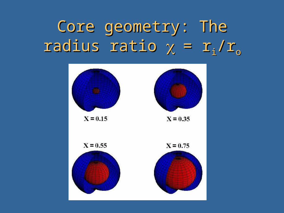
Core geometry: The radius ratio Core geometry: The radius ratio = r= rii/r/roo

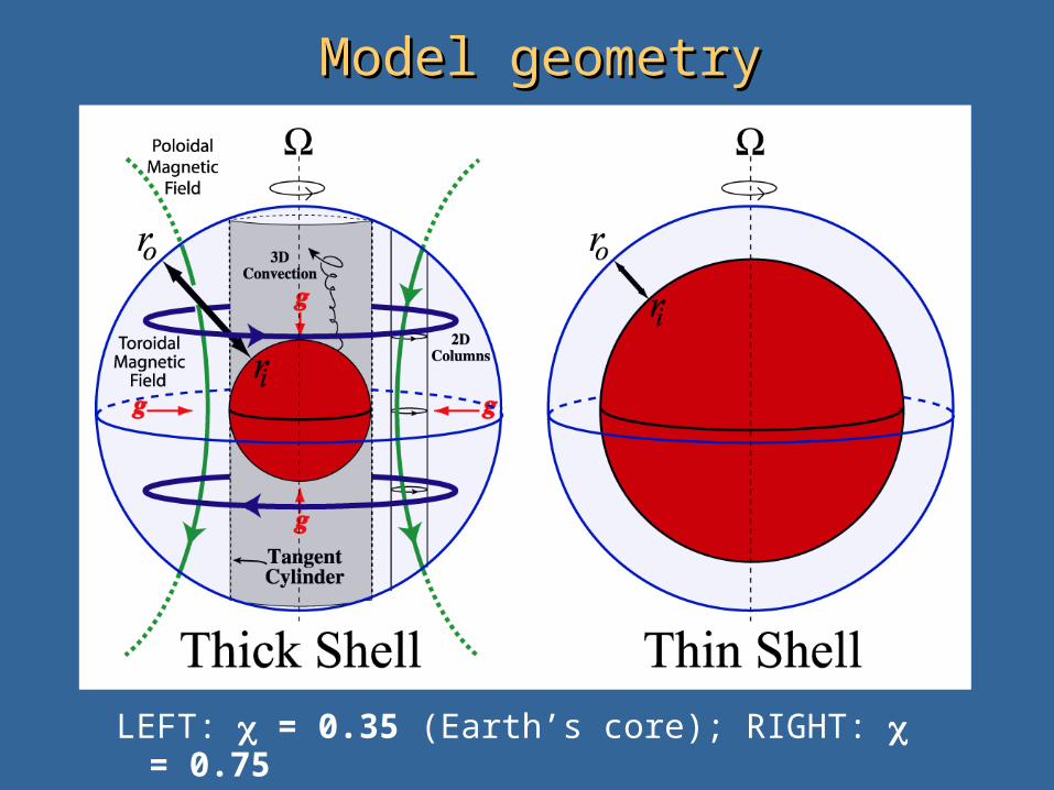
Model geometryModel geometry

LEFT: = 0.35 (Earth’s core); RIGHT: = 0.75

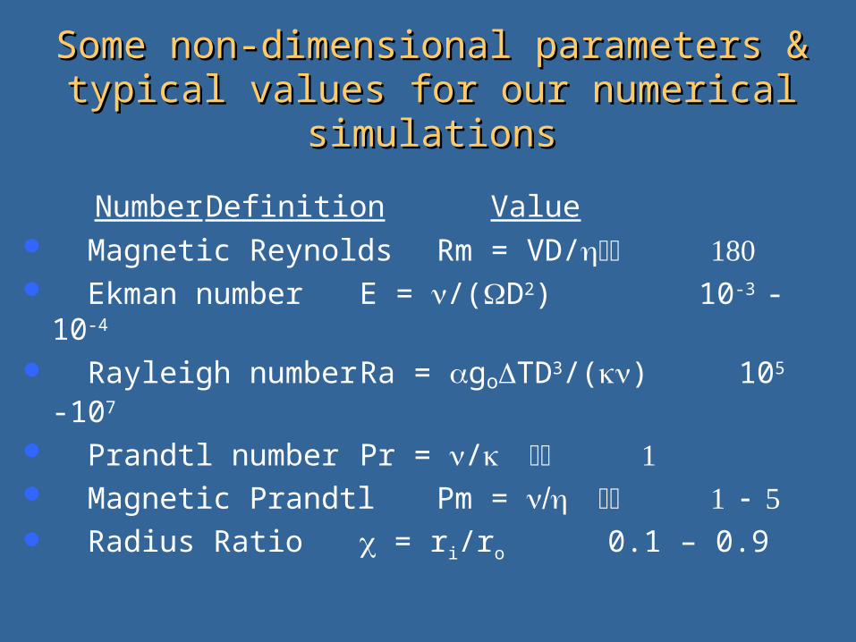
Some non-dimensional parameters & typical Some non-dimensional parameters & typical values for our numerical simulationsvalues for our numerical simulations

Number Definition Value Magnetic Reynolds Rm = VD/ Ekman number E = /(D2) 10-3 -10-4

Rayleigh number Ra = goTD3/() 105 -107

Prandtl number Pr = / Magnetic Prandtl Pm = Radius Ratio = ri/ro 0.1 – 0.9

Spherical dynamo codeSpherical dynamo code Originally developed by G. Glatzmaier. Modified by U. Christensen and J. Wicht. We are presently running a slightly modified

version of the Wicht code, called Magic2. Spectral transform code. Latitudinal and

longitudinal directions expanded with spherical harmonics. Chebychev polynomials in radius.

Time stepping via Courant criterion using a grid representation .

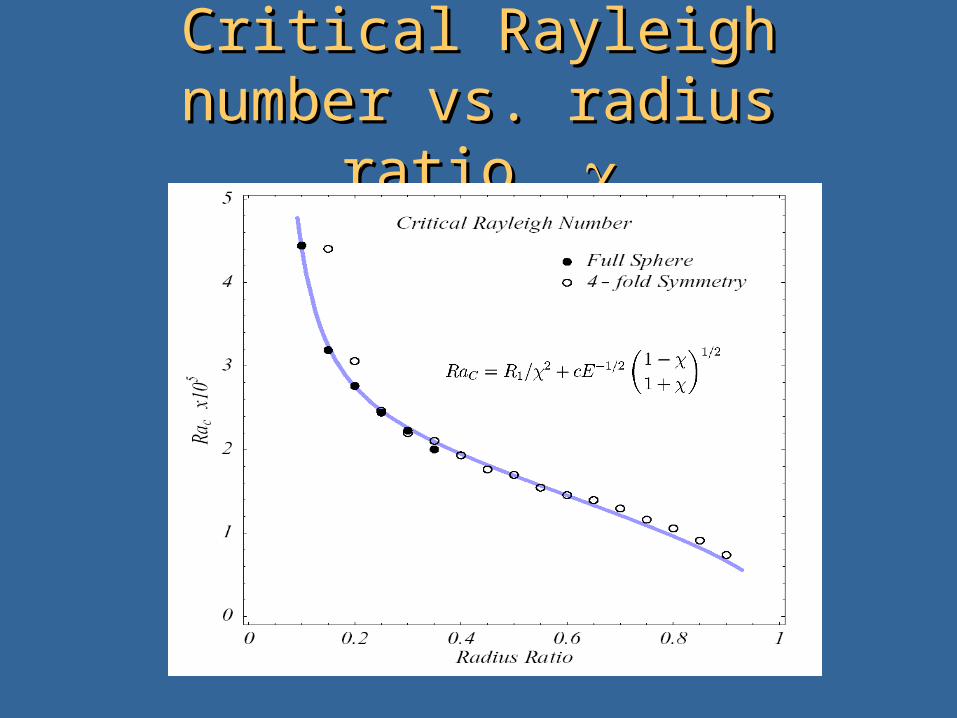
Critical Rayleigh number vs. Critical Rayleigh number vs. radius ratio, radius ratio,

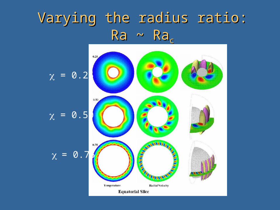
Varying the radius ratio: Ra ~ RaVarying the radius ratio: Ra ~ Racc

= 0.25

= 0.50

= 0.75

Number of Taylor Columns is Number of Taylor Columns is proportional to the radius ratioproportional to the radius ratio

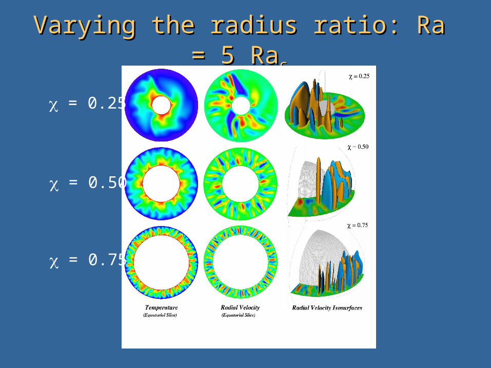
Varying the radius ratio: Ra = 5 RaVarying the radius ratio: Ra = 5 Racc

= 0.25

= 0.50

= 0.75

Critical Rayleigh number for Critical Rayleigh number for dynamo actiondynamo action

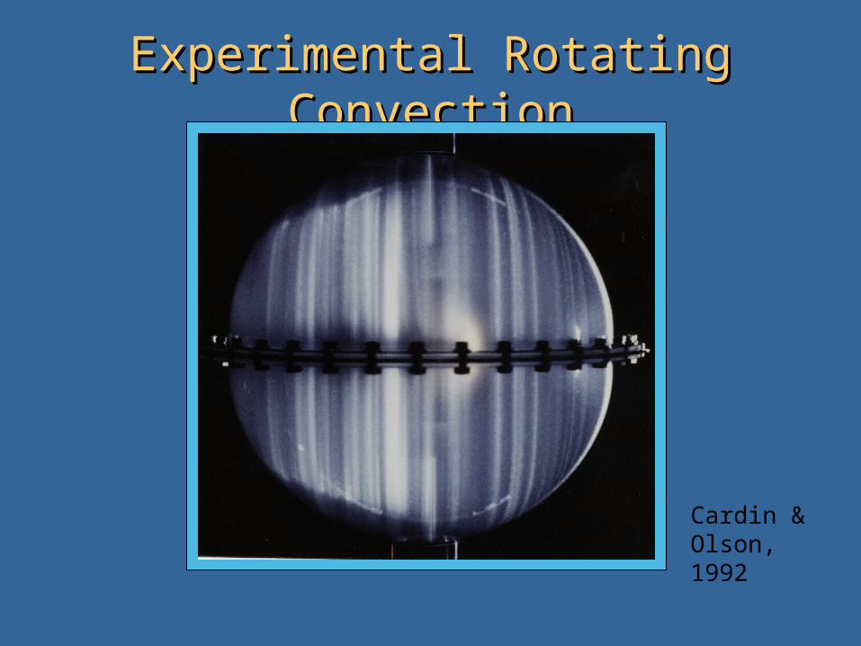
Experimental Rotating ConvectionExperimental Rotating Convection

Cardin & Olson, 1992

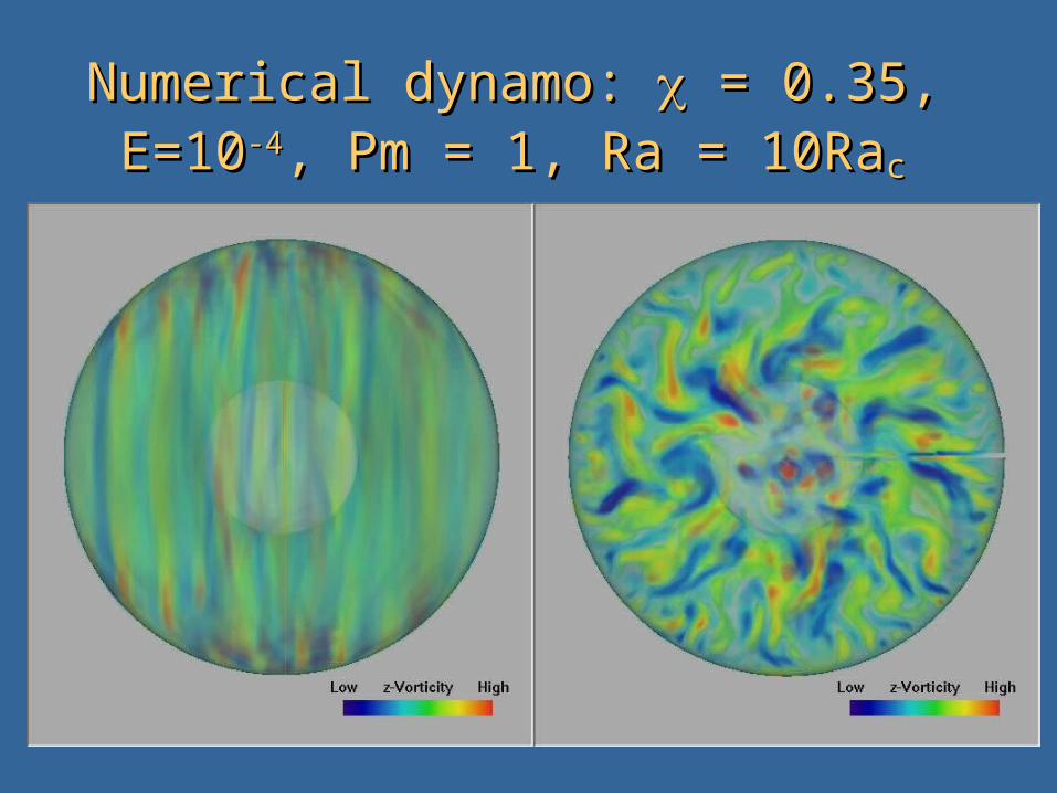
Numerical dynamo: Numerical dynamo: = 0.35, = 0.35, E=10E=10-4-4, Pm = 1, Ra = 10Ra, Pm = 1, Ra = 10Racc

Real time visualization:Real time visualization:MotivationMotivation

Writing and storage of solutions more expensive than running simulation

Interactive adjustment of run parameters can save calculation time

Fast processing and data transfer makes real time feasible

Visual immersion helps interpretation of dynamical structures.

data com data com

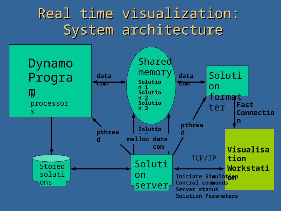
Real time visualization: Real time visualization: System architectureSystem architecture

Dynamo ProgramN processors

Solution server

Stored solutions

Visualisation Workstation

Shared memorySolution 1Solution 2Solution 3...Solution m

Solution formatter

TCP/IP

Fast Connection

Initiate SimulationControl commandsServer statusSolution Parameters

malloc data com

pthreadpthread

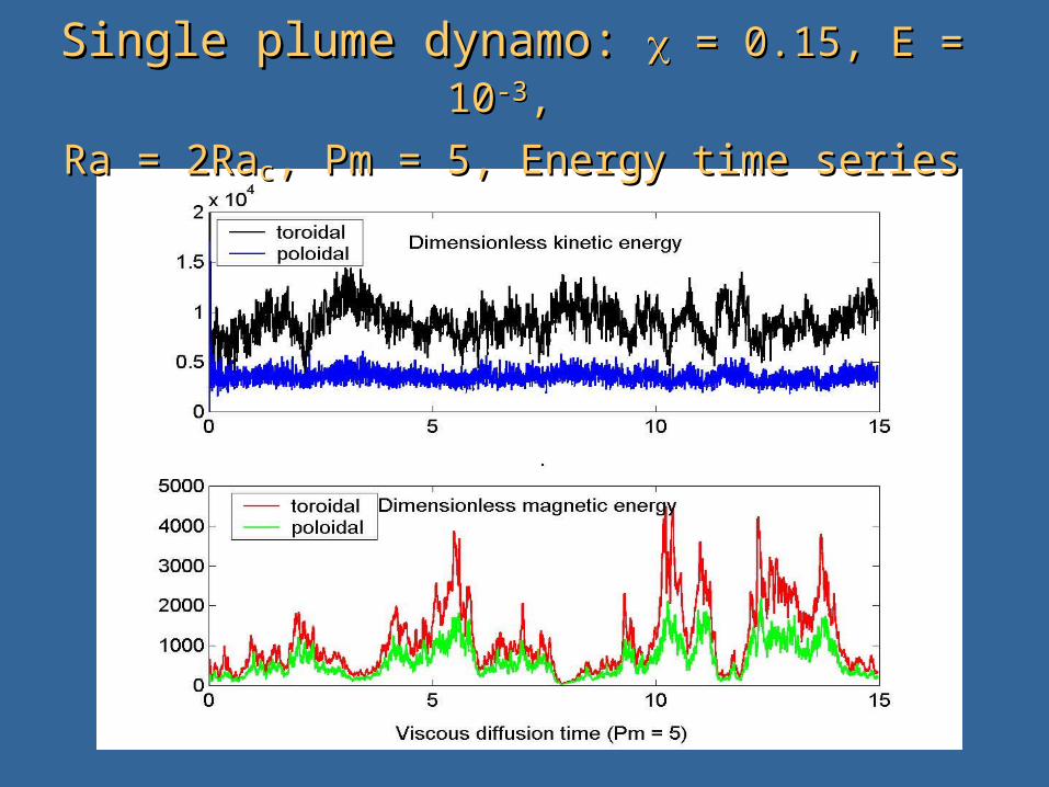
Single plume dynamo: Single plume dynamo: = 0.15, E = 10 = 0.15, E = 10-3-3, ,

Ra = 2RaRa = 2Racc, Pm = 5, Energy time series, Pm = 5, Energy time series

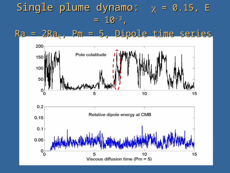
Single plume dynamo: Single plume dynamo: = 0.15, E = 10 = 0.15, E = 10-3-3, ,

Ra = 2RaRa = 2Racc, Pm = 5, Dipole time series, Pm = 5, Dipole time series

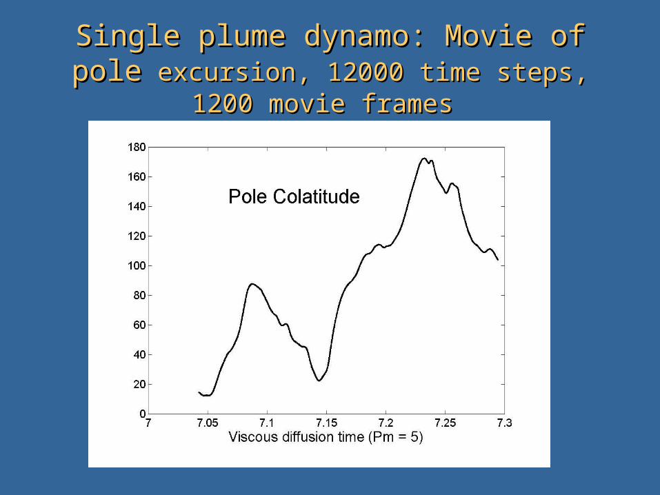
Single plume dynamo: Movie of poleSingle plume dynamo: Movie of pole excursion, 12000 time steps, 1200 movie frames excursion, 12000 time steps, 1200 movie frames

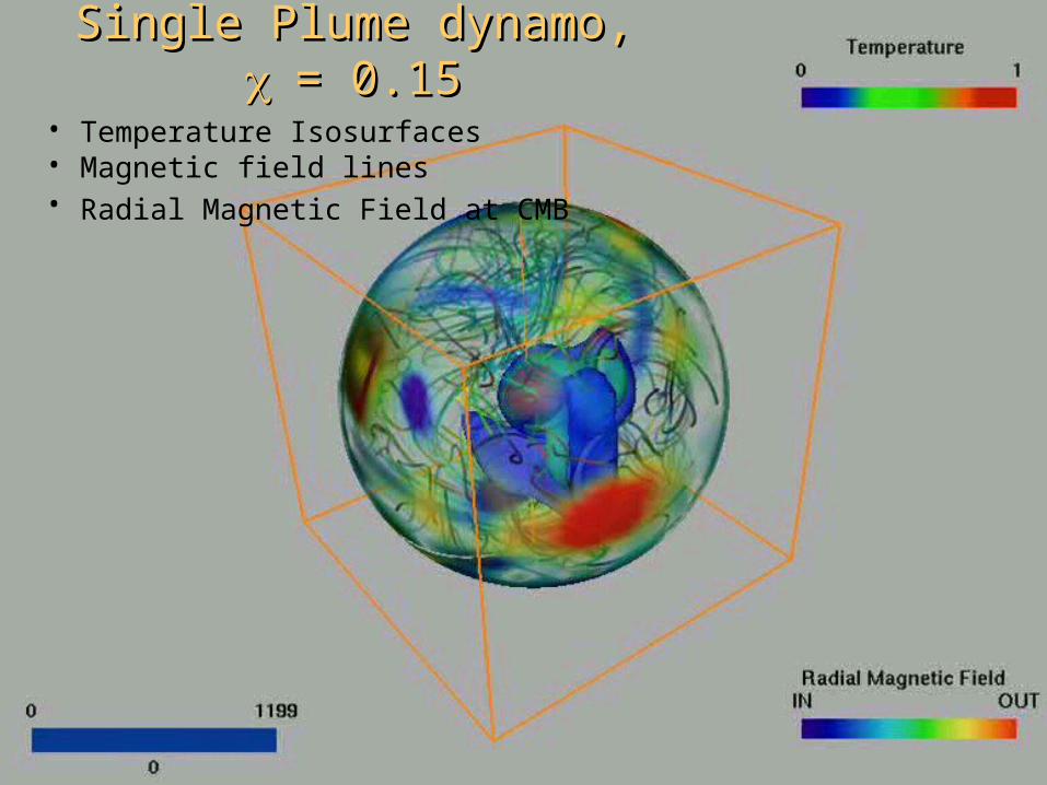
Single Plume dynamo, Single Plume dynamo, = = 0.150.15

• Temperature Isosurfaces• Magnetic field lines• Radial Magnetic Field at CMB

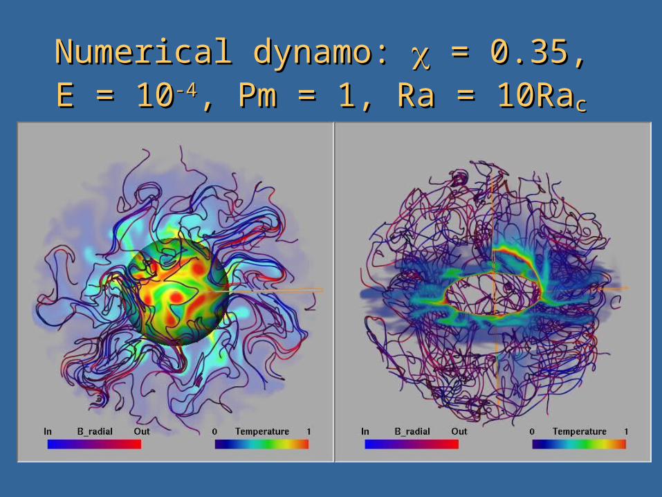
Numerical dynamo: Numerical dynamo: = 0.35, = 0.35, E = 10E = 10-4-4, Pm = 1, Ra = 10Ra, Pm = 1, Ra = 10Racc

Real time visualization:Real time visualization:ObjectivesObjectives

Create a virtual sensory environment that helps the human brain to analyze numerical dynamos.– Bring the benefits of the experimental lab to the

numerical laboratory

Steering of numerical runs– Adjust parameters during a run

– Adjust visualization tools (e.g. inject tracer particles)

Independence of visualization system from computational code

– Adaptation to various computational codes