1

Working Paper #20

AN ANALYTICAL APPROACH TO ACTIVATING

DEMAND ELASTICITY WITH A

DEMAND RESPONSE MECHANISM

Cédric CLASTRES and Haikel KHALFALLAH

02.11.2015

2

AN ANALYTICAL APPROACH TO ACTIVATING DEMAND ELASTICITY WITH A DEMAND RESPONSE MECHANISM

Cédric Clastres1,* and Haikel Khalfallah2

ABSTRACT The aim of this work is to demonstrate analytically the conditions under which activating the elasticity of consumer demand could benefit social welfare. We have developed an analytical equilibrium model to quantify the effect of deploying demand response on social welfare and energy trade. The novelty of this research is that it demonstrates the existence of an optimal area for the price signal in which demand response enhances social welfare. This optimal area is negatively correlated to the degree of competitiveness of generation technologies and the market size of the system. In particular, it should be noted that the value of un-served energy or energy reduction which the producers could lose from such a demand response scheme would limit its effectiveness. This constraint is even greater if energy trade between countries is limited. Finally, we have demonstrated scope for more aggressive demand response, when only considering the impact in terms of consumer surplus.

Keywords: Demand Response, Price Signals, Welfare Analysis. JEL Classification: C61, L11, Q41.

1. INTRODUCTION

The deployment of smart grids is seen as heralding a major change in electricity markets. One of the main considerations, presented as a necessary condition to benefit from this development, is to be able pilot demand or make it respond to price or market constraints (Chao, 2011). Setting aside any improvements in network management, consumer behaviour will have a KEY impact on uses and investment-planning in the midstream (networks) and the upstream (generation) (Strbac, 2008). The idea is to replace some of the heavy investment in infrastructure by a reduction in consumption. This could be done by consumers or another body (aggregators, suppliers, distributors) on behalf of consumers. Experiments have shown that investing in smart-grid technology could be cheaper than heavier investments in infrastructure (Kema, 2012).

The main feature of electricity demand is its inelasticity (Stoft, 2002). Currently, most electricity consumers are captive in the short term. Industrial customers could be more volatile, but mainly in the long term (Lijesen, 2007; Patrick and Wolak, 1997). However the aim of deploying smart grids and demand-response (DR) schemes is to introduce short-term elasticity into some uses. In this way, issuing price signals to consumers will always reduce consumption3. The literature generally shows that demand is elastic when a dynamic tariff is introduced. However, the value of the elasticity varies depending on several factors, such as the period of consumption, household appliances, degree of deployment of smart-grid technologies, or the price differential between periods of consumption (Di 1 Associate Professor, University of Grenoble, EDDEN-UPMF and CEEM Research Fellow (Université Paris

Dauphine) , +33 4 56 52 85 78, cedric.clastres@upmf-grenoble.fr 2Associate Professor, University of Grenoble, EDDEN-UPMF, +33 4 56 52 85 80, haikel.khalfallah@upmf-

grenoble.fr * This paper has benefited from the support of the Chaire European Electricity Markets of the Paris Dauphine Foundation, supported by RTE, EDF, EPEX Spot and the Group Caisse des dépôts. The views and opinions expressed in this Working Paper are those of the authors and do not necessarily reflect those of the partners of the CEEM. 3 This result could be overcome by extending the rebound effect (Muratori et al., 2014).

3

Cosmo et al., 2014; Boisvert et al. 2004; Faruqui and Sergici, 2010). Several papers have studied the impact of dynamic pricing on consumers and markets design to remunerate curtailments. Chao (2011) has demonstrated that, in a perfect competitive market, remuneration of curtailment equals to the difference between the retail rate and the real-time price should be optimal for welfare. Orans et al. (2010) show that a three-part tariff, including time-of-use, a fixed fee and DR remuneration, is an efficient tool for providing consumers with an incentive to change their behaviour.

We draw on these papers using analytical equilibrium in interconnected markets to study the cases in which an increase in tariffs would reduce consumption without jeopardizing social welfare. We use a deterministic optimization model with supply functions (Ventosa et al., 2005). As in other papers (Stoft, 2002), we assume perfect competitive markets. Each producer bases its bids on its marginal costs, as in Woo (1990) and De Jonghe et al. (2011). However, to our knowledge, only a few works have sought to model analytically deployment of demand response in the context of interconnected electricity markets. Vespucci et al. (2013) is the model closest to ours. A large part of their analysis focuses on the transformation of their optimization problem into a linear one, as electric supply and demand functions are discontinuous.They also demonstrate, with application data, that a dominant firm always has an incentive to use market power to achieve higher profit targets. Our model differs from theirs on two points. Firstly, we compute theoretical equilibriums in the context of two interconnected markets with several technologies in each market. Secondly, we introduce an analysis of Demand Response (DR) linked to the degree of the elasticity of consumer demand. Léautier (2014) has also studied, using an analytical approach, the impacts on welfare of switching from inelastic to elastic demand via the application of Real Time Pricing scheme4. Our analysis extends this work by addressing the effectiveness of Demand Response when several markets, using different generation technologies, are interconnected. It adds to this literature on considering the extent to which the effectiveness of a Demand Response should consider the system’s interactions with foreign systems through the energy exchanges and the difference between the generation technologies mix.

In our research work, we focus on the effectiveness of deploying a Demand Response scheme. We may assume that widespread application of DR would have several impacts on system equilibrium. The main objective of this scheme is to make consumers sensitive to prices in the short run5. They could actively participate in managing system security, instead of relying only on supply management when the system is close to rationing. DR schemes offer consumers an incentive to adopt a degree of flexibility in their consumption. Each part of the electricity supply chain would benefit from this flexibility, gaining in efficiency.

Deploying a mechanism of this sort would nevertheless have a high cost. Consumers need to adapt and modify their behaviour, switching from being captive and non-elastic to being genuinely elastic. It is worth noting that under a DR scheme, demand becomes elastic for a large range of consumers, independently of their own appliances. As several pilot schemes in the US have shown (Faruqui et al., 2009), the main gains are obviously achieved at peak hours. Demand for electrical heating or air conditioning are the main categories of consumption which could be managed under DR schemes. However, dynamic pricing gives a large share of consumers an incentive to reduce consumption, regardless of whether they own air conditioning, for example (Di Cosmo et al., 2014). Information

4 Leautier (2014) applies his results to the French market. As marginal revenue of SG deployment is decreasing,

current costs of marginal deployment of smart meters are too high compared to benefits. Thus, it should be not profitable to continue to install equipment for all consumers. Moreover, Crampes and Leautier (2015) have recently shown that under imperfect information, DR could reduce the welfare from the adjustment market as consumers could behave strategically. 5 Electricity consumers are recognized to be elastic only in the long run, even if in the short run, some of them

can be partly elastic too. We also note that we make no distinction between residential and industrial consumers, who have different consumption profiles and would in practice react differently to an intensive DR scheme.

4

technology, such as home displays, increases such effects, providing continuous information to customers on consumption and tariffs. The impact of DR schemes on price bids has been studied in the literature. DR is a key factor in making smart grids work because it allows efficient interaction between the segments of the electricity supply chain6. The literature has studied a variety of DR tools (Bergaentzlé et al., 2014; Faruqui and Sergici, 2010; Horowitz and Lave, 2014), going from the simplest mechanism which involves dividing periods of consumption into price blocks, in which the price increases in step with short-term system vulnerability (Time-Of-Use or Critical Peak Pricing), to more complex systems in which consumers respond to electricity prices in real time (Real Time Pricing). When several communications technologies are developed, load management of consumers by the supplier or the Distribution System Operator would allow a significant decrease in demand, higher than a reduction managed only by the consumer. All these tools imply an increase in electricity prices at times of high demand and lower prices at other times. It seems realistic to assume that activating DR will result in an increase in electricity prices in peak periods. As prices increase, some consumers could be worse off due to this increase (Horowitz and Lave, 2014). As the main gain from a DR scheme is a drop in peak-load demand, incentive prices or direct load control are used to make the volume effect greater than the price effect, in other words decreasing electricity consumption compensates for increasing prices. This should be done by minimizing the impact on consumer utility7, as consumers must have incentives to participate in a DR scheme. We shall therefore study two economic indicators – social welfare and consumer surplus – to gauge the efficiency of the DR schemes.

In our paper, we model a system in which generators, integrated with suppliers or retailers, make bids (supply curves) to the system operator which maximizes the welfare balancing offer and demand. With SG technologies, consumers could become active on the market; thus their demand function becomes elastic. In this environment, we start by analysing the way the structure of generating technologies could affect merit orders in different countries and potential trade between them. Our results show that the trade-off between producing locally and exporting energy depends on the opportunity cost of the energy and the overall efficiency of generating technologies. Then we demonstrate that there is an optimal level for the price signal at which DR increases social welfare. We use computed equilibria from our initial analysis to show that this optimal level is negatively correlated to the degree of competitiveness of the generating technologies and the size of the market. The value which producers could lose due to unserved energy or energy reductions would limit deployment of a scheme of this sort. Moreover this constraint is greater if energy trade between countries is limited. However the constraint is less acute if the considered system is cost-inefficient, with only limited connections with neighbouring systems.

The paper is divided into five sections. Following this introduction, Section 2 presents the assumptions used in modelling the analytical equilibriums and results of social-welfare analysis. Section 3 focuses on the effectiveness of DR with regard to consumer-surplus criteria. Section 4 analyses the sensitivity of the results to the elasticity of demand. Section 5 presents our conclusions.

6 For instance generators of conventional or intermittent energies could easily manage variations in their

production and integrate renewable energies in the power system. 7 One of the main fields of research by suppliers is for ways of convincing consumers to participate in DR

schemes. To gain consumer acceptance, DR schemes must minimize impact on both modern amenities and electricity bills.

5

2. A MODEL FOR DEMAND RESPONSE

2.1. General Assumptions

2.1.1. Trade between the systems

We shall assume there are two interconnected countries8 (n=1,2)9. Each system operator balances total supply and demand making allowance for possible trade between the countries. Such trade is limited by an interconnection capacity between country n and m, 𝐶𝑎𝑝𝑛,𝑚, which has a price 𝑃𝑛,𝑚

when capacity is saturated.

2.1.2. Generation technologies and supply

Each country is characterized by the presence of t generation technologies, t=1..k. We assume perfect competition in both markets10. Each technology is characterized by a quadratic variable cost function11, described as follows:

𝐶𝑉𝑡,𝑛(𝑥𝑡,𝑛) = 𝑎𝑡,𝑛. 𝑥𝑡,𝑛 +1

2. 𝑏𝑡,𝑛. 𝑥𝑡,𝑛

2 (1)

𝑎𝑡,𝑛 and 𝑏𝑡,𝑛 are parameters and 𝑥𝑡,𝑛 is the quantity produced by technology t in a given country n.

By aggregating the marginal costs of the technologies available in country n, we obtain the following inverse supply function:

𝑆𝑛(𝑋𝑛) = 𝑎𝑛 + 𝑏𝑛𝑋𝑛 (2)

𝑎𝑛 and 𝑏𝑛 are aggregate parameters and 𝑋𝑛 = ∑ (𝑥𝑡,𝑛𝑘𝑡=1 + 𝑥𝑡,𝑛,𝑚) is the total quantity produced in a

given country n, with 𝑥𝑡,𝑛,𝑚 the quantity produced by technology t in a given country n and exported

towards country m. See Appendix 1 for more details on construction of the supply function.

For simplicity’s sake we shall rank the technologies from the least to the most expensive12. A linear relationship between the variable costs function of the technologies is made as follows:

𝑎𝑡,𝑛 = 𝛼𝑡−1. 𝑎 and 𝑏𝑡,𝑛 = 𝛼

𝑡−1. 𝑏

Where 𝛼 is a ranking parameter of the technologies13; 𝑎 and 𝑏 correspond to the parameters of the least expensive technology.

2.1.3. Demand and market equilibrium

In the first scenario, electricity demand in a given country is assumed to be inelastic (𝐷𝑛). In the second scenario, we assume that implementing a Demand Response mechanism will modify

8 The model could be enlarged to analyze more than two interconnected systems.

9 Index m is also used.

10 We disregard the strategic behaviour of producers by assuming that the merit order of a given system is the

result of aggregating the marginal costs of available generation technologies. The model is a one-shot game with linear demand. To serve demand all capacities are offered to the market through the aggregate supply function. 11

Assuming a perfect competitive market, fixed generation costs are disregarded, having no impact on our results. 12

The efficiency of generation technologies relies on input costs, yields, others variable costs to produce one MWh, costs of Emission Trading System, the period of use, etc. 13

We assume that 𝛼 is slightly >1 to keep a rational homogeneity in the generation technologies and avoid exponential disparity between them.

6

consumer behaviour, so that demand becomes elastic. The inverse demand function in the latter case is given by:

𝐷𝑛−1(𝑋𝑛) = 𝑐𝑛 − 𝑑𝑛. 𝑋𝑛 (3)

Where 𝑐𝑛 and 𝑑𝑛 are the parameters of the inverse demand function.

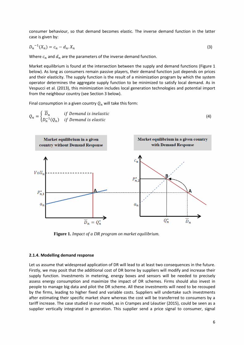
Market equilibrium is found at the intersection between the supply and demand functions (Figure 1 below). As long as consumers remain passive players, their demand function just depends on prices and their elasticity. The supply function is the result of a minimization program by which the system operator determines the aggregate supply function to be minimized to satisfy local demand. As in Vespucci et al. (2013), this minimization includes local generation technologies and potential import from the neighbour country (see Section 3 below).

Final consumption in a given country 𝑄𝑛 will take this form:

𝑄𝑛 = 𝐷𝑛 𝑖𝑓 𝐷𝑒𝑚𝑎𝑛𝑑 𝑖𝑠 𝑖𝑛𝑒𝑙𝑎𝑠𝑡𝑖𝑐

𝐷𝑛−1(𝑄𝑛) 𝑖𝑓 𝐷𝑒𝑚𝑎𝑛𝑑 𝑖𝑠 𝑒𝑙𝑎𝑠𝑡𝑖𝑐

(4)

2.1.4. Modelling demand response

Let us assume that widespread application of DR will lead to at least two consequences in the future. Firstly, we may posit that the additional cost of DR borne by suppliers will modify and increase their supply function. Investments in metering, energy boxes and sensors will be needed to precisely assess energy consumption and maximize the impact of DR schemes. Firms should also invest in people to manage big data and pilot the DR scheme. All these investments will need to be recouped by the firms, leading to higher fixed and variable costs. Suppliers will undertake such investments after estimating their specific market share whereas the cost will be transferred to consumers by a tariff increase. The case studied in our model, as in Crampes and Léautier (2015), could be seen as a supplier vertically integrated in generation. This supplier send a price signal to consumer, signal

Figure 1. Impact of a DR program on market equilibrium.

7

composed by smart appliances costs and others features of the market. Without loss of generality, we could normalise retail costs to 0. As perfect competition is assumed, the supply function of the integrated entity should integrate supply costs plus costs of smart appliances that should be recovered through its supply activity14. Finally, these costs are paid by consumers. Thus, this could be modelled by assuming that the technology’s operational costs (Equation 1 above) will increase by a

convex function, 1

2γ𝑛. 𝑥𝑡,𝑛

2 where γ𝑛 can be interpreted as a DR intensity parameter15. This

parameter contains all costs of the DR program as well as the intensity of the price signal given to consumers. We therefore assume a positive correlation between the intensity of suppliers’ investments in the smart-grid system and the opportunity for consumers to manage their consumption with a wide range of tools (in-home-display, direct load control, energy boxes, etc.). On the other hand, we can assume that consumers, now being price sensitive, will become demand-elastic. Graphically, the electricity price shifts from point A to point B, as shown in Figure 1 above, as it moves from a no-DR scenario to a widespread-DR scenario. With deployment of smart grids, consumers receive information, allowing them to make decisions, change their patterns of electricity consumption and adapt their demand. DR schemes change the cost of electricity for consumers: they receive new price signals, given by their suppliers, and, with new SG technologies, they can respond to them. The reserve price for consumers with DR, 𝑐𝑛, is now higher than 𝑉𝑜𝑙𝑙𝑛. Indeed when consumer demand is price-elastic, consumers are inclined to pay higher prices for electricity when the system is rationed, so they attach a much higher value to electricity scarcity which implies an increase in the value of lost energy (Voll) 16.

We shall consequently study the impact of price-based DR on the market equilibrium of two interconnected areas, with regard to social welfare and consumer surplus. We first consider the most the system operator can reduce demand without any loss in social welfare. We define 𝑄𝑛,𝑚𝑖𝑛 as the

minimum consumption we can reach without decreasing social welfare. Then, we introduce analysis of consumer surplus to show that some types of DR scheme may not degrade this surplus. We also carry out sensitivity analysis of key parameters and the level of demand elasticity. 2.2. Welfare-related analysis of the impact of demand response

2.2.1. Baseline case We start from the scenario without demand response. Since demand is inelastic, optimal production and trade maximizing social welfare (5) are the solution of the following program:

𝑀𝑎𝑥𝑥𝑡,𝑛,𝑥𝑡,𝑛,𝑚 ∫ (𝑉𝑜𝑙𝑙𝑛 − 𝑆𝑛(𝑋𝑛))𝑑𝑋𝑛𝐷𝑛0

(5)

Subject to,

14

Several operators or actors could invest in smart technologies or smart appliances: suppliers/retailers, consumers, aggregators of flexibility, etc. Our model only considers the investment made by suppliers. We do

not capture those made by aggregators or directly by consumers. Smart Grid investments can be seen as any other classical investment in innovation. It’s firstly assumed by suppliers or grid companies and then passed through to consumers via an increase in the regulated tariffs or directly in electricity prices. Moreover, pilot on smart grids have shown that utilities make the investment that is more often a private one (with a complement of public funds). An exception is on smart meters that are supported by DSO. However, in the following sections, we could present some intuitions on the case in which consumers have made these investment. We are grateful to an anonymous referee for this remark improving the understanding of the research. 15

The more the investment in smart appliances is, the more the demand response could be high. The degree of smart investment is positively correlated to the potential of DR. Thus, γn captures this relationship and its meaning could be analysed as the intensity of DR program. 16

In practice, the reserve price varies with the type of consumers, their elasticities as well as the duration of the outage (Leautier 2012).

8

𝑥𝑡,𝑛 + 𝑥𝑡,𝑛,𝑚 ≤ 𝐾𝑡,𝑛 (𝑟𝑡,𝑛)

∑ 𝑥𝑡,𝑛,𝑚𝑡 ≤ 𝐶𝑎𝑝𝑛,𝑚 (𝑃𝑛,𝑚)

(6)

(7)

∑ 𝑥𝑡,𝑛 + ∑ 𝑥𝑡,𝑚,𝑛 = 𝑄𝑛𝑡𝑡 (𝑓𝑛) (8)

Where,

𝐶𝑎𝑝𝑛,𝑚 Interconnection capacity between country n and country m

𝑋𝑡,𝑛 = 𝑥𝑡,𝑛 + 𝑥𝑡,𝑛,𝑚 Total generation of technology t in country n

𝐾𝑡,𝑛 Available installed capacity of technology t in country n

𝑄𝑛 Final consumption in country n

Energy generation in a given country must comply with two constraints. First, the quantity generated by each technology t, which includes local generation, 𝑥𝑡,𝑛, and possible exports to the neighbour country, 𝑥𝑡,𝑛,𝑚, cannot exceed available installed capacity (equation 6). Secondly, energy exports from country n to country m are limited by the capacity of the interconnection line, 𝐶𝑎𝑝𝑛,𝑚 in equation 7. Finally, equation 8 shows that each system must balance its market by aligning local consumption, 𝑄𝑛, with total energy fed into the system.

To solve the above constrained program, the equilibrium determines the optimal generation quantities, 𝑥𝑡,𝑛

∗ and 𝑥𝑡,𝑛,𝑚∗ , which simultaneously minimize the variable costs of generation in both

countries. As demonstrated in Appendix 2, the solution is unique since the cost functions are strictly convex and continuously differentiable. The solution is found by regrouping all first-order conditions to form a mixed complementarity problem17.

Resolving the model as demonstrated in Appendix 3 implies the following main results:

Proposition 1 The trade-off between producing locally or exporting energy would depend on the opportunity cost of energy and the overall efficiency of the production technology. Interconnection prices in both directions would limit trade between the countries. This impact is however weighted by the generation-costs differential between interconnected markets.

Optimal levels of production are defined as follows:

𝑥∗𝑡,𝑛 − 𝑥∗𝑡,𝑛,𝑚 =

𝑄𝑛−𝑄𝑚𝛼𝑡−1

𝛼−1

+(1−𝛼).∑ 𝑃𝑛,𝑚𝑛

𝛼𝑡−1.(1−𝛼𝑡).𝑏. ∑

1

𝛼𝑚𝑡−1𝑡 (9)

Proof. See Appendix 3

When local consumption is higher than consumption in the foreign country: 𝑄𝑛 ≥ 𝑄𝑚, the production which meets local demand 𝑥∗𝑡,𝑛 is far higher than the quantity exported 𝑥∗𝑡,𝑛,𝑚. In this

case, the opportunity cost of selling energy to the local market is higher than exporting. Moreover, we can observe that the efficiency of the technology t compared to the other technologies would

17

Complementarity problems can be seen as expansions of square systems of nonlinear equations that include a mixture of equations and inequalities. It solves directly the necessary conditions of the mathematical programs. It solves directly the necessary conditions of the mathematical programs. Writing and solving the first order optimality conditions simultaneously for all programs results in a mixed complementarity problem.

9

influence the trade-off between producing locally and exporting. We assume that 𝜔𝑡 =𝛼𝑡−1

𝛼−1 is the

overall efficiency factor of technology t. This term 𝜔𝑡 also provides information on price levels in the two markets which balance supply and demand. So, according to this term, producers in country n must export capacity when their technologies are more efficient than those of their competitors in country m. The greater the efficiency of technology t, i.e. 𝜔𝑡 decreases, the more it will be preferred for balancing the system of the country with higher energy consumption.

The high values of 𝑃𝑛,𝑚 reduce the incentives for country n to export. The influence of the interconnection-capacity price on generation decisions is weighted by the efficiency factor of the

technologies in the importing country defined by: ∑1

𝛼𝑚𝑡−1𝑡 . Thus, to maximize social welfare, it would

be beneficial for country m with inefficient technologies to rely more on imports even with substantial interconnection prices, leading to an increase in 𝑥∗𝑡,𝑛,𝑚.

Proposition 2: Efficient technologies would be called first to balance the markets. Other technologies would satisfy residual demand depending on their overall and relative efficiency. Trade would however be strongly correlated to interconnection prices and cost intensity in the importing country. Each efficient technology t would offer all its installed capacity to the interconnected markets. Optimal quantities for local production and for export are given as follow18:

𝑥∗𝑡,𝑛 =𝐾𝑡,𝑛

2+𝑄𝑛−𝑄𝑚

2.𝜔𝑡+∑ 𝑃𝑛,𝑚𝑛 .∑

1

α𝑡,𝑚𝑡

𝑏.𝜔𝑡 (10)

𝑥∗𝑡,𝑛,𝑚 =𝐾𝑡,𝑛

2−𝑄𝑛−𝑄𝑚

2.𝜔𝑡− ∑ 𝑃𝑛,𝑚𝑛 .∑

1

α𝑡,𝑚𝑡

𝑏.𝜔𝑡 (11)

We define 𝑡 as the index of inefficient technologies. They would only serve residual demand in the interconnected markets, with quantities lower than their total installed capacity. Their optimal production levels are given by19:

𝑥∗𝑡,𝑛 =𝑅𝑒𝑠𝑛−ɸ𝑡𝜔𝑡

+𝑃𝑚,𝑛

𝑏.𝜔𝑡. ∑

1

α𝑡,𝑚𝑡 (12)

𝑥∗𝑡,𝑛,𝑚 =𝑅𝑒𝑠𝑚−ɸ𝑡

𝜔𝑡−𝑃𝑛,𝑚

𝑏.𝜔𝑡. ∑

1

α𝑡,𝑚𝑡 (13)

Where, 𝑅𝑒𝑠𝑛 = 𝑄𝑛 −∑ 𝑥∗𝑡,𝑛𝑡 − ∑ 𝑥∗𝑡,𝑚,𝑛𝑡 𝑅𝑒𝑠𝑚 = 𝑄𝑚 −∑ 𝑥∗𝑡,𝑚𝑡 − ∑ 𝑥∗𝑡,𝑛,𝑚𝑡

𝜔𝑡 =𝛼𝑡−1

𝛼−1 where 𝑡 is the index of an inefficient technology

ɸ𝑡 = ∑𝑎𝑡,𝑛−𝑎,𝑛

𝑏𝑡,𝑛 where 𝑡 is the index of the other inefficient technologies apart from 𝑡

Proof. See Appendix 4

The call for a given technology to produce would depend on its efficiency compared to other technologies. When its efficiency is higher than a certain threshold, as discussed in Appendix 4, all its available capacity will be used to balance the systems. The other technologies will either fulfil the efficiency conditions and will hence be called at full capacity, or only serve residual demand, thus verifying the solution of equation 12 and 13.

18

Providing 𝑥∗𝑡,𝑛 and 𝑥∗𝑡,𝑛,𝑚 are non-negative, with 𝑥∗𝑡,𝑛 + 𝑥∗𝑡,𝑛,𝑚 < 𝐾. Otherwise, if 𝑥∗𝑡,𝑛 + 𝑥

∗𝑡,𝑛,𝑚 ≥ 𝐾𝑡,𝑛,

the equilibrium is 𝑥∗𝑡,𝑛 + 𝑥∗𝑡,𝑛,𝑚 = 𝐾𝑡,𝑛 and others technologies serve residual demand.

19 Providing 𝑥∗𝑡,𝑛 and 𝑥∗𝑡,𝑛,𝑚 are non-negative and their sum does not exceed the technology capacity 𝐾𝑡,𝑛.

Otherwise, inefficient technologies produce at full capacity and there is a risk of an unbalanced market with no equilibrium.

10

We shall now consider the efficient technologies. We can see that the share of capacity between local production and export is mainly determined by the energy-consumption differential, 𝑄𝑛 − 𝑄𝑚. Generation is symmetrically shared between local generation and export, with a constant slope

which depends on the overall efficiency factor of the technology, 1

2.𝜔𝑡; the total cannot exceed the

available generation capacity, 𝐾𝑡,𝑛. If technology t of country n is efficient with respect to other technologies, its production increases to serve both local demand and exports to neighbouring country m until its full capacity 𝐾𝑡,𝑛 is reached. Generation sharing is impacted by the overall

efficiency factor of the technology, 𝜔𝑡. An increase in 𝛼𝑡−1, which means that the technology tends to be more costly, leads to an increase in 𝜔𝑡, meaning that the technology becomes less efficient. In this case, the incurred inefficiency will be borne by the system facing low demand. This behaviour should stop as soon as the overall inefficiency factor of efficient technology reaches a limit beyond which the technology becomes absolutely inefficient and will hence be shared, given the solutions to equations 12 and 13. As for inefficient technologies, their call is increasingly dependent on residual demand, as shown in equations 12 and 13, and on the overall, 𝜔𝑡 , and relative, ɸ𝑡 , efficiencies of the technology compared to the other inefficient ones. Not surprisingly, when choosing between inefficient technologies, the least inefficient ones are preferred, so 𝑥∗𝑡,𝑛 and 𝑥∗𝑡,𝑛,𝑚 decrease when 𝜔𝑡 or ɸ𝑡

increase. However potential export is only impacted directly by the export capacity price, 𝑃𝑛,𝑚. System operators will only rely slightly on inefficient generation technologies to balance their systems, so these technologies will only serve as auxiliary capacity.

In sections and subsections that follow, the analysis of welfare, consumer surplus and elasticity will use the results of the equilibrium computed in equations (10-13) and also refer to figure 1. Indeed, this figure illustrates how the elasticity of demand, consumer surplus and welfare levels could be modified given different parameters of costs, the level of market size and two configuration regarding the transmission capacity limits.

2.2.2. Introducing demand response

To assess the social efficiency of a DR scheme, we consider the maximum level of demand reduction the system operator can achieve without loss of social welfare. As we said above, we define 𝑄𝑛,𝑚𝑖𝑛 as the minimum consumption above which social welfare does not decrease. As our model is on a single period, we could not capture the effect of load-shifting across several periods when DR occurs20. We assume that the efficiency of a DR scheme would also depend on the competitiveness of the country concerned. We consequently consider two extremes cases separately: a cost-efficient country scenario; and a cost-inefficient country scenario.

The results of the previous sub-section highlight the impact of the opportunity cost of energy and the cost efficiency of technologies on energy trade between countries, subject to interconnection-capacity prices. The trade-off between costs and volume efficiencies would drive decisions on trade and generation. In the following we apply these theoretical predictions by considering the particular case of elastic demand with DR. The results of proposition 1 and 2 will serve as the analytical basis for the following efficiency study.

We define 𝛥𝑛 as the variation in welfare after deploying a DR scheme in country n as follows: 𝛥𝑛 = 𝑆𝑊𝑛,2 − 𝑆𝑊𝑛,1 (14)

20

However, load-shifting leads to greater demand in others periods. Thus, the demand function 𝐷𝑛−1(𝑋𝑛) =

𝑐𝑛 − 𝑑𝑛 . 𝑋𝑛 moves upward, increasing SWn,2. In our model, this increase in demand decreases Qn,min. Obviously, this effect relies on the fact that demand stays elastic. If we compare SWn,1 and SWn,2, an increase in demand increases Qn,min; thus shifting demand from one period to another one could be detrimental for welfare.

11

Where,

𝑆𝑊𝑛,1 = ∫ (𝑉𝑜𝑙𝑙𝑛 − 𝑆𝑛(𝑋𝑛))𝑑𝑋𝑛𝐷𝑛0

: social welfare at equilibrium before deploying the DR scheme.

𝑆𝑊𝑛,2 = ∫ (𝐷𝑛−1(𝑋𝑛) − 𝑆𝑛(𝑋𝑛))𝑑𝑋𝑛

𝑄𝑛∗

0 : social welfare at equilibrium after deploying the DR

scheme.

Developing the above function, we obtain that 𝛥𝑛 ≥ 0, i.e. DR is socially efficient, when the equilibrium quantity is in the optimal area defined below:

𝑄𝑛∗ ≥ 𝑄𝑛,𝑚𝑖𝑛 =

2.𝑆𝑊𝑛,1

𝑐𝑛−𝑎𝑛 (15)

𝑄𝑛∗ is the equilibrium effectively reached according to the supply and demand functions and the DR

parameter, γ𝑛. 𝑄𝑛,𝑚𝑖𝑛 is the minimum equilibrium quantity which could be reached with a DR

scheme without a decrease in social welfare. This threshold exists for each equilibrium 𝑄𝑛∗ , i.e. for all

configurations of the supply and demand functions. According to the supply and demand parameters, some of these equilibriums will induce a positive variation in social welfare.

As we also know that at intersection point B in Figure 1, 𝑄𝑛∗ =

𝑐𝑛−𝑎𝑛

γ𝑛+𝑏𝑛+𝑑𝑛, we can obtain a negative

correlation between the intensity of the DR scheme, γ𝑛, and the probability of coping with 𝛥𝑛 ≥ 0 as lim𝛾𝑛→+∞ 𝑄𝑛

∗ = 0. This result makes sense, since the greater the intensity of DR, the more

consumption is reduced. It being optimal for the DR scheme to reach 𝑄𝑛∗ ∈ [𝑄𝑛,𝑚𝑖𝑛, 𝑄𝑛,𝑚𝑎𝑥 =

𝑐𝑛

𝑑𝑛] to

maintain social-welfare gains, intensive DR should have a greater impact reducing both consumer surplus and the profits of firms which base their competitive strategy on their marginal costs. There is consequently no incentive to design a γ𝑛 such as 𝑄𝑛

∗ < 𝑄𝑛,𝑚𝑖𝑛 because of social-welfare losses

when the demand function is elastic21. As 𝛥𝑛 is an increasing function of 𝑄𝑛, we could conclude that 𝑄𝑛∗ = 𝑄𝑛,𝑚𝑖𝑛 is the minimal condition the equilibrium must meet to keep the gains from DR schemes.

According to this initial result, we can see that the minimum quantity is linked to the parameters of the supply function 𝑎𝑛 and 𝑏𝑛, reflecting the marginal costs of supply, and reserve electricity prices before and after changes in consumer behaviour due to the DR scheme, 𝑉𝑜𝑙𝑙𝑛 and 𝑐𝑛 respectively.

2.2.2.1. Efficient country results

Proposition 3 If the country is efficient, there is an optimal area for which a demand response scheme does not reduce social welfare. This area is negatively correlated with the degree of competitiveness of the generation technologies and the size of the country’s market.

The intuition of proposition 3 is the following. A large size of the market increases Qn,min. Indeed, if Kt,n increases, a cheap generation is then available to serve the demand. Thus SWn,1 will increase too.

In the same way, high levels of 𝐷𝑛 increases SWn,1. As a result, Qn,min increases, which implies difficulties to achieve the condition SWn,2 > SWn,1. Moreover, in this case, a great DR deteriorates profits of efficient generators because of the non-served energy. The price effect does not compensate loses in sales in the retail market (as DR reduces final demand). Consumers’ surplus is also damaged because of rationing whereas cheaper generation is available to serve their demand22. Cheaper generation goes with higher SWn,1. Here again, the condition SWn,2 > SWn,1 is difficult to achieve. Thus opportunities to improve welfare with cheap generation capacities are reduced.

21

Assuming that consumers make the smart investment, leading to a function dn(γ𝑛), this does not change our

intuitions if 𝑑(𝑑𝑛(γ𝑛))

𝑑(γ𝑛)> 0, an assumption we reasonably assume. Moreover, the impact on 𝑄𝑛

∗ stays the same,

only the optimal interval [𝑄𝑛,𝑚𝑖𝑛 , 𝑄𝑛,𝑚𝑎𝑥] is reduced. 22

Chao (2011) has shown similar results by considering incentives policies of DR to consumers. He concludes that if remuneration of DR is too high (called the « double remuneration »), it could be detrimental for welfare because DR is over-evaluated, by replacing a cheaper generation which is more efficient.

12

From other side, DR reduces the demand in efficient country n. Thus, efficient generators are willing to increase their exports towards inefficient country m. However, if costs of interconnectors are high (or if transmission capacity is limited), they could not easily increase their export levels. Thus, Qn,min will increase. Moreover, the efficiency of the overall interconnected market is reduced, a large part of the residual demand being served by inefficient or less efficient generation.

To sum up, DR programs could reduce the welfare when generation technologies are efficient. A high level of inelastic demand or large efficient generation capacities increase these loses (because of high initial values of SWn,1). High level of DR could be implemented only if costs parameters bn are high or

for low values of Dn (that have a decreasing impact on SWn,1).

To demonstrate these results, we assume first that country n is more efficient than country m. This means that with or without price signals, only its generation technologies will be called to meet local demand.

Integrating our results from Proposition 2 into equation (15), the optimal minimum quantity is thus equal to:

𝑄𝑛,𝑚𝑖𝑛 =∑ 𝐾𝑡,𝑛𝑡 −𝛼.𝑄𝑚+

𝑃𝑛,𝑚(𝛼−1).𝑏

2−𝛼=2.𝑆𝑊𝑛,1

𝑐𝑛−𝑎𝑛 (16)

The left term (from cost-minimization program (5-8)) and the right term (from equation 15) are equal at equilibrium. Any change in a parameter of one term will be accompanied by a proportional change in another parameter in the other term, guaranteeing that the above equality always holds and equilibrium is still the one in which efficient technologies are predominant. The link between the two terms is obtained through parameter 𝑏𝑛 as it is detailed below23.

We can deduce from equation (16) that the borders of the optimal area depend on many parameters related to the configuration of the interconnected systems and technology specifications. We define three criteria to study the sensitivity of 𝑄𝑛,𝑚𝑖𝑛 to the main parameters. The first one concerns the

market size of the efficient country. It is impacted by 𝐾𝑡,𝑛 and 𝐷𝑛. Indeed the greater these parameters become, the larger we may assume the system to be. The second indicator is the level of cost efficiency of technologies. Parameters such as supply-function parameters, 𝑎𝑛 and 𝑏𝑛 fall into this category. The third indicator reflects the impact of the limitation on transmission capacity.

Market size

From equation 16, we observe that an increase in the size of the efficient country’s market, either

due to an increase in ∑ 𝐾𝑡,𝑛𝑡 or in 𝐷𝑛, causes 𝑄𝑛,𝑚𝑖𝑛 to increase, consequently reducing the optimal area of DR. Two reasons could explain this correlation. First, because country n is cheap, any increase in its technology capacity will lead, on the one hand, to an increase in the level of exports to country m and, on the other, will offer cheaper technologies to country n, reducing the slope of its energy mix (parameter 𝑏𝑛) and boosting initial social welfare 𝑆𝑊𝑛,1. We thus obtain an identical increase on the left and right sides of equation 16. The optimal area of a DR scheme, which does not degrade

social welfare, is therefore reduced24. Secondly, the higher initial demand is, 𝐷𝑛25, the greater the

reduction in generation required to cope with the DR target (for lower consumption). The impact on the profitability of producers is consequently negative, due to the higher value of their unused

23

This analysis procedure is followed for all the scenarios below.

24 𝑑(∑ 𝐾𝑡,𝑛𝑡 −𝛼.𝑄𝑚

2−𝛼)

𝑑𝐾𝑡,𝑛> 0 if 𝛼.

𝑑𝑄𝑛,𝑚𝑖𝑛

𝑑𝑐𝑛<1, meaning that only part of the capacity increase will be exported. At the

same time, 𝑑𝑆𝑊𝑛,1

𝑑𝐾𝑡,𝑛> 0 because of decrease in 𝑏𝑛.

25 𝑑𝑆𝑊𝑛,1

𝑑𝐷𝑛> 0 because 𝑃𝑛,1

∗ = 𝑎𝑛 + 𝑏𝑛𝐷𝑛 < 𝑃𝑛.

13

capacity. As for consumers, a higher 𝐷𝑛 means that captive demand is high enough to allow rationing of a large number of users by a DR scheme, without impacting negatively on their welfare.

As a preliminary conclusion, we may assume that intensive DR is constrained by the market size of the system because of the considerable impact on producers of the value of non-served energy. Consumer rigidity would not only undermine the efficiency of DR, it would also impact the producers, with a drop in profit. In this case, consumer rationing is costly for society. There is no need for consumers to be rationed or adapt their consumption, generation being available and cheap. Indeed, the loss in terms of surplus could be very high in a situation where generation is cheap but consumption must decrease because of the voluntary price increase. There is a kind of opportunity cost for rationing consumers without constraining the system.

System-cost efficiency

The second group of parameters regarding cost efficiency comprises parameters specific to the supply function (𝑎𝑛 and 𝑏𝑛). Again, when 𝑎𝑛 or 𝑏𝑛 decreases, which also means that technologies are

increasingly efficient, we observe an increase in 𝑄𝑛,𝑚𝑖𝑛. Indeed the cost of serving demand 𝐷𝑛 with an efficient energy mix is now lower. Intensive DR would entail a higher opportunity cost which in turn would limit DR efficiency.

Transmission-capacity limit

Due to the constraint on interconnection capacity, a capacity price effect associated with use of the

interconnection is represented by 𝑃𝑛,𝑚

(𝛼−1).𝑏. The higher the value of interconnection capacity, the

smaller the optimal DR area becomes. Intensive DR should encourage consumers to greatly reduce their consumption. Such a reduction in consumption will be accompanied by a large drop in local generation. However, efficient producers, seeing a huge reduction in the volume they generate, can export surplus production to the less efficient neighbouring country, thus reducing the negative volume effect of such a measure. But when interconnection capacity is limited and access to it is more expensive, export becomes both more costly and less feasible. Hence, the equilibrium at which the greatest possible use is made of efficient technologies is much more difficult to reach. The cost of serving rationed demand will significantly increase, prompting the system operator to adopt a less intensive DR scheme to prevent system collapse.

Optimal system configuration for intensive demand response

To conclude we shall look at two indicators reflecting the cost structure and the market size of the studied country. The first one includes, as stated previously, parameters such as the supply-function parameters, 𝑎𝑛 and 𝑏𝑛. As we have shown, the impact of these parameters on 𝑄𝑛,𝑚𝑖𝑛 is the same:

the more cost-efficient technologies are, the higher 𝑄𝑛,𝑚𝑖𝑛 becomes. So, for simplicity’s sake, we can focus exclusively on parameter 𝑏𝑛, as a good indicator of the cost efficiency of the technologies.

Regarding the market size indicator, we should emphasize that the higher initial captive demand 𝐷𝑛, or generation capacity ∑ 𝐾𝑡,𝑛𝑡 , is, the higher 𝑄𝑛,𝑚𝑖𝑛 becomes. For greater simplicity, we shall centre

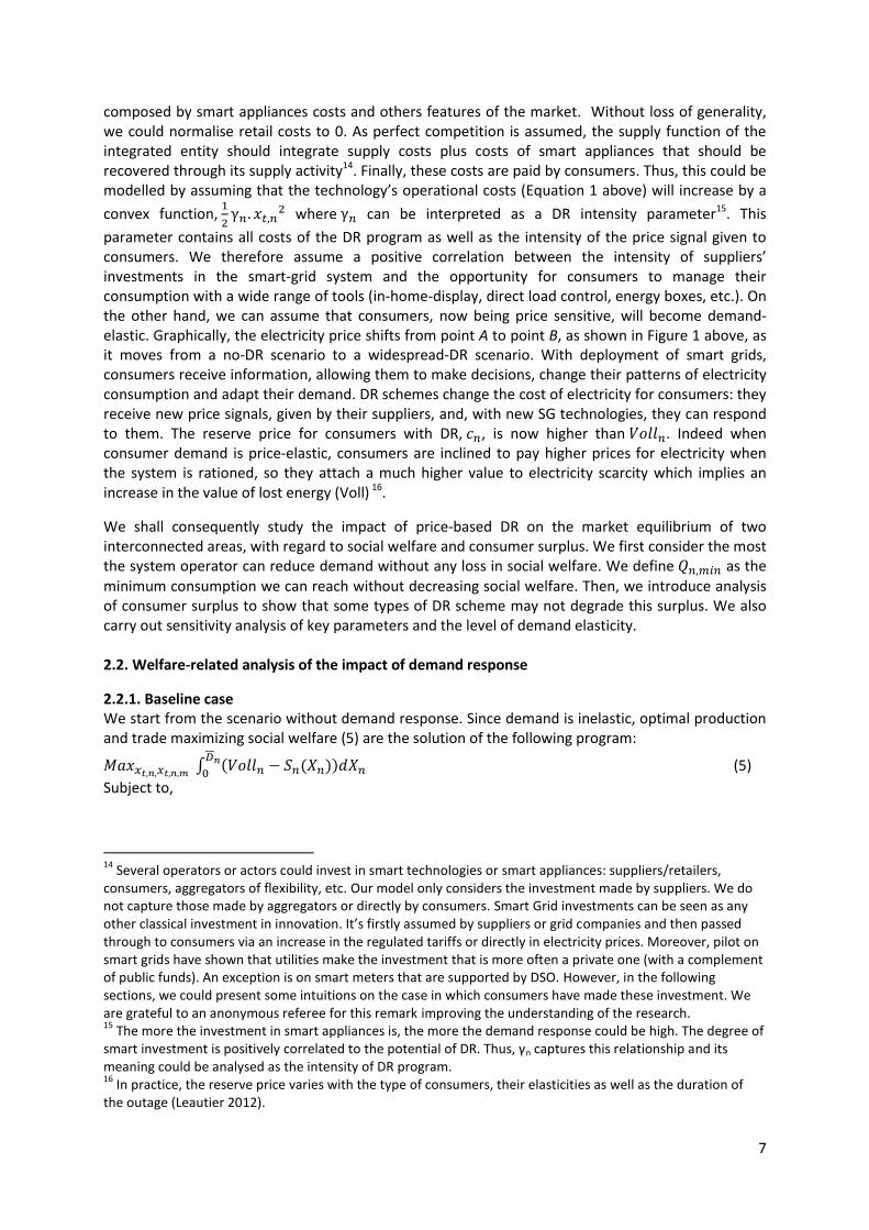
our conclusion on the impact of 𝐷𝑛. Figure 2 below shows the variation in the optimal area

depending on the levels of 𝑏𝑛 and 𝐷𝑛26. The curves are approximated, based on our results from

equations 15 and 16.

Two zones can be identified. The first zone A means that with low 𝑏𝑛 and low 𝐷𝑛, it is not possible substantially to reduce demand. If 𝑏𝑛 is sufficiently low, rationing will lead to a high negative price

26

We disregard extreme situations, i.e. when country become inefficient compared to its neighbour. Such situation will be studied in the next sub-section.

14

effect on consumers. With low demand, the scheme would not yield a significantly positive quantity effect. In the opposite case, if both parameters are high, the volume effect is considerable compared to the price effect. In other words, the drop in generation yields an initial effect, with a second effect caused by the higher value of unused capacity. Finally, a slight reduction in demand is also expected

when 𝑏𝑛 is low and 𝐷𝑛 high. Whereas the positive volume effect for consumers would be offset by the high negative price effect, producers would lose a large amount of their surplus, as in the previous case because of the significant drop in generation reduction and higher value of unused capacity. However the positive impact of the price increase on producers would be limited, given the increasing impact of the DR scheme on operating costs.

However, an aggressive DR scheme could only be deployed if 𝑏𝑛 was high and 𝐷𝑛 low (zone B in Figure 2). To more reduce consumption without welfare losses, the negative volume effect of the DR scheme on consumers and producers must be offset by the positive price effect, yielding an insignificant impact on total surplus.

2.2.2.2. Inefficient country

Proposition 4 If a country is inefficient, the more it imports, the less effective intensive DR will be.

The intuitions of proposition 4 are as follows. Costs and Dn have the same impact as in the previous case (efficient country). However, imports are playing now a major role. We could see the DR intensity is a decreasing function of imports from the efficient country. Indeed, if these imports are large, thus SWn,1 is great which makes difficult to satisfy SWn,2 > SWn,1. We could conclude that if

Figure 2. Optimal regions of DR for efficient country

15

interconnection prices are high (or for low interconnection capacities), the DR could also be high (SWn,1 is reduced and the condition SWn,2 > SWn,1 is easily satisfied). A more aggressive DR could also be implemented if bn is high (reflecting high generation cost in country n) or for low values of Kt,m (imports from efficient country are reduced). Indeed, in that case, consumers are served by costly generation. If they cannot import cheaper energy, thus SWn,1 is reduced and Qn,min decreases, facilitating the satisfaction of SWn,2 > SWn,1.

To demonstrate these results, we shall now assume that country n is less efficient than country m. This means that with or without price signals, it always relies on imports from country m to satisfy local demand.

The minimum quantity for efficient DR is equal to:

𝑄𝑛,𝑚𝑖𝑛 =∑ 𝐾𝑡,𝑚𝑡 −𝛼.𝑄𝑚−

𝛼2

𝛼−1.𝑏.∑ 𝑃𝑚,𝑛𝑚 +𝑅𝑒𝑠𝑛

2−𝛼=2.𝑆𝑊𝑛,1

𝑐𝑛−𝑎𝑛 (17)

Parameters 𝑎𝑛 and 𝑏𝑛 (through 𝑆𝑊𝑛,1) have the same effect on 𝑄𝑛,𝑚𝑖𝑛. Any decrease in the

inefficiency of the cost of the technologies positively impacts 𝑄𝑛,𝑚𝑖𝑛. Similarly the market-size

indicator of the inefficient country, 𝐷𝑛, through 𝑆𝑊𝑛,1, stills positively influences 𝑄𝑛,𝑚𝑖𝑛. The optimal area is however significantly influenced by the market size of the exporting country m, i.e. 𝐾𝑡,𝑚, as we will see next. As a preliminary interpretation, we can say that since the country relies massively on imports, any local energy policy would be subject mainly to the attractiveness of imports.

Market size of the exporting country

When the level of generation capacity in the exporting country, 𝐾𝑡,𝑚, rises, so does 𝑄𝑛,𝑚𝑖𝑛. DR in the inefficient importing country becomes less effective. An increase in 𝐾𝑡,𝑚 will relax the neighbouring

system, therefore encouraging higher exports to the inefficient system. Two situations are consequently possible. The inefficient technologies in country n may be more replaced by less costly ones, so that an increase in 𝐾𝑡,𝑚 will be accompanied by a decrease in the residual demand served by local producers, 𝑅𝑒𝑠𝑛, with quite limited impact on 𝑄𝑛,𝑚𝑖𝑛. Alternatively the growth in capacity in

the exporting country will be transferred to country n, thus satisfying more demand. 𝑄𝑛,𝑚𝑖𝑛 must increase because 𝑅𝑒𝑠𝑛 will still be unchanged. In the latter case, rationing is more harmful for consumers. Indeed, when available capacity is competitive, consumers do not need to be rationed or adapt their consumption, generation being cheap. The opportunity cost of rationing consumers without constraining the system is significant here.

Transmission-capacity limit

Equation 17 shows that the greater the cost of imports for the inefficient country, the more intensive DR could be. Indeed, when 𝑃𝑚,𝑛 increases, there is less scope for relying on imports to satisfy local demand. Inefficient local generation will be used to balance the system. Given that the opportunity cost of reducing generation is much lower for inefficient technologies (local producers) than efficient ones (exporters), the system operator can deploy a more aggressive DR scheme without facing the social cost of unserved generation entailed by relying only on efficient technologies.

Optimal system configuration for intensive demand response

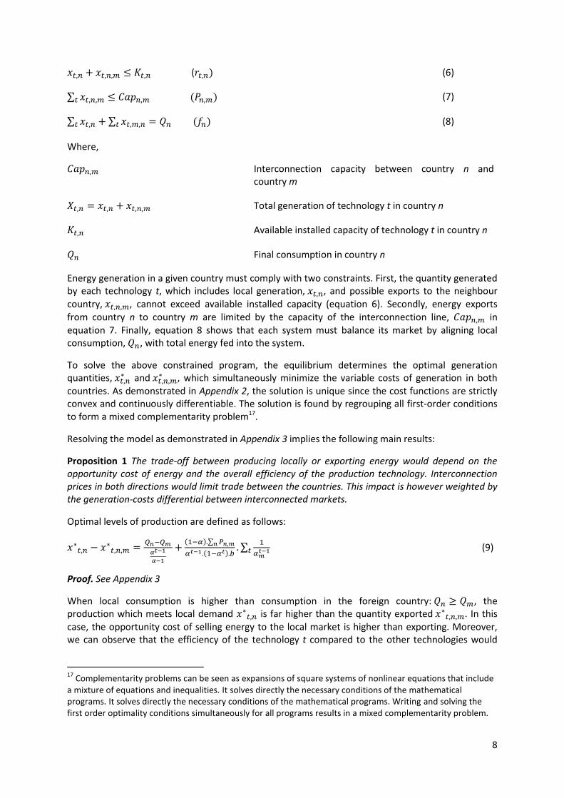
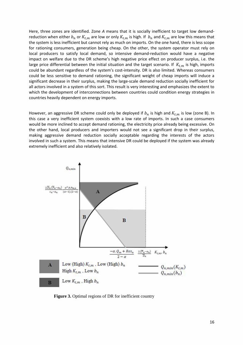
To conclude, we shall again focus on two criteria relating to the cost level of technologies in the inefficient country and to the market size of the exporting country, given that it significantly influences equilibrium in the studied market. We consider the parameter 𝑏𝑛 as an indicator of the country’s efficiency. We look at the impact of 𝐾𝑡,𝑚 as an indicator of the market size of the neighbouring country counterbalancing the inefficiency of the studied country. Figure 3 below shows the optimal area of DR with regard to 𝑏𝑛 and 𝐾𝑡,𝑚.

16

Here, three zones are identified. Zone A means that it is socially inefficient to target low demand-reduction when either 𝑏𝑛 or 𝐾𝑡,𝑚 are low or only 𝐾𝑡,𝑚 is high. If 𝑏𝑛 and 𝐾𝑡,𝑚 are low this means that

the system is less inefficient but cannot rely as much on imports. On the one hand, there is less scope for rationing consumers, generation being cheap. On the other, the system operator must rely on local producers to satisfy local demand, so intensive demand-reduction would have a negative impact on welfare due to the DR scheme’s high negative price effect on producer surplus, i.e. the large price differential between the initial situation and the target scenario. If 𝐾𝑡,𝑚 is high, imports

could be abundant regardless of the system’s cost-intensity. DR is also limited. Whereas consumers could be less sensitive to demand rationing, the significant weight of cheap imports will induce a significant decrease in their surplus, making the large-scale demand reduction socially inefficient for all actors involved in a system of this sort. This result is very interesting and emphasizes the extent to which the development of interconnections between countries could condition energy strategies in countries heavily dependent on energy imports.

However, an aggressive DR scheme could only be deployed if 𝑏𝑛 is high and 𝐾𝑡,𝑚 is low (zone B). In this case a very inefficient system coexists with a low rate of imports. In such a case consumers would be more inclined to accept demand rationing, the electricity price already being excessive. On the other hand, local producers and importers would not see a significant drop in their surplus, making aggressive demand reduction socially acceptable regarding the interests of the actors involved in such a system. This means that intensive DR could be deployed if the system was already extremely inefficient and also relatively isolated.

Figure 3. Optimal regions of DR for inefficient country

17

These results are summarized in the table 1 below.

Table 1: Impact of DR programs on welfare with efficient or inefficient country

Welfare improvement with DR No welfare improvement with DR

Efficient country (n)

Low values of Kt,n or 𝐷𝑛 High values of costs or Pn,m

High values of Pn,m, Kt,n or 𝐷𝑛 Low values of costs

Inefficient country (n)

High values of Pn,m High values of costs and low values of Kt,m

High values of Kt,m or low values of Kt,n Low values of costs and Kt,m

3. CONSUMER-SURPLUS ANALYSIS

We shall now study the extent to which the optimal area for DR schemes would vary if, instead of social welfare, we consider variations in consumer surplus. Consumers are sensitive to financial losses that could occur with the adoption of a new technology (Park et al., 2014). In the case of a smart grid being deployed with demand-response schemes and dynamic pricing, these fears would be associated with lower surplus, because of the risk of higher electricity bills27. This is one of the main risks that consumer groups fear when DR schemes are introduced. Indeed, a DR mechanism must act mainly on consumer profiles; its efficiency depends on their willingness to adapt and the elasticity the DR scheme can activate. The impact on consumer surplus is a major social constraint which the authorities should take into account when trying to modify the rational equilibrium of their energy systems.

Proposition 5. If variation in consumer surplus, rather than social welfare, was used as the key criterion, more aggressive DR could be adopted, unless the system was cost-inefficient and captive demand is low.

Intuitively, if consumer’s demand is high, they could reduce it easier. Moreover, for costly generation technologies, their energy bills are high. Thus, consumers would modify their consumption (they decrease it) to reduce their payments. Choosing greater values of γ𝑛 would be optimal, as we made the assumption of the positive correlation between the level of investment costs in smart appliances and demand reduction. With a consumers surplus analysis, loses of the generators’ side are not considered, leading then to sustain the benefits of greater demand response.

To show these results, we define Ω𝑛 as the variation in consumer surplus after deploying a DR scheme:

Ω𝑛 = 𝐶𝑆𝑛,2 − 𝐶𝑆𝑛,1 (18)

𝐶𝑆𝑛,1 = ∫ (𝐷𝑛)𝑑𝑃𝑛𝑉𝑜𝑙𝑙𝑛𝑃𝑛∗ : consumer surplus at equilibrium before deploying a DR scheme.

𝐶𝑆𝑛,2 = ∫ (𝐷𝑛(𝑃𝑛))𝑑𝑃𝑛𝑐𝑛𝑃𝑛∗ : consumer surplus at equilibrium after deploying a DR scheme.

Developing the above function28, we obtain that Ω𝑛 ≥ 0, i.e. DR is efficient from the consumers’ point of view, when the equilibrium quantity falls within the optimal area below:

𝑄𝑛∗ ≥ 𝑄𝑛,𝑚𝑖𝑛 = √

2.𝐶𝑆𝑛,1

𝑑𝑛 (19)

27

SG and DR pilots have shown that this risk exists but could be limited for consumers who react to signals from utilities or DSOs (Faruqui et al., 2007 ; Faruqui et al., 2011 ; Faruqui and Sergici, 2010).

28 Ω𝑛 ≥ 0 if 𝑄𝑛 . (

𝑐𝑛−𝑃𝑛

2) ≥ 𝐶𝑆𝑛,2. Given that 𝑃𝑛 = 𝑐𝑛 − 𝑑𝑛 . 𝑄𝑛, then 𝑄𝑛,𝑚𝑖𝑛 = √

2.𝐶𝑆𝑛,1

𝑑𝑛.

18

It would be possible to reduce consumption without decreasing consumer surplus as far as 𝑄𝑛,𝑚𝑖𝑛 in

equation 19 above. We can verify that DR intensity is positively correlated to elasticity of the demand function and negatively correlated to captive-demand prices. If we assume that the authorities mainly consider the impact in term of consumer surplus, we can demonstrate that a higher reduction in consumption could be obtained if the following condition was met29:

√2.𝐶𝑆𝑛,1

𝑑𝑛≤2.𝑆𝑊𝑛,1

𝑐𝑛−𝑎𝑛 (20)

In what follows, we shall look at the additional reduction in consumption which could be achieved subject to a consumer-surplus constraint, by focusing on two parameters: the system’s cost

efficiency and market size, respectively 𝑏𝑛 and 𝐷𝑛30. The results shown in Figure 4 confirm our

previous results regarding the impact of consumer surplus on variation in social welfare, via the price and the volume effects of the DR scheme. The figure yields two main conclusions. First, when the

market size of the system is high, i.e. high 𝐷𝑛as shown is the right-hand part of Figure 4, and regardless of the level of cost efficiency, a higher reduction in consumption could be reached if only the impact on consumer surplus is considered (zone B in the right-hand part of Figure 4). This additional reduction in quantity could also be obtained if demand was moderate, but the system must be highly inefficient in terms of cost (zone B in the left-hand part of the figure). Indeed, if demand is very high, the negative price effect of intensive DR on consumers would be off-set by the positive volume effect. On the other hand, for producers, the positive price effect being insignificant (price variation is low due to the additional cost of DR), the negative price effect would substantially reduce their own surplus. DR could consequently not be intensive. Likewise, if demand was not high enough, DR could only be intensive if the system was expensive. In which case, consumers already paying high bills would be more inclined to accept aggressive demand reduction, the volume effect being higher than the price effect.

The second conclusion is that, with an approach focusing on consumer surplus, we cannot expect a major reduction in consumption if the system is already cheap and demand is low (zone A in the figure). Again, the negative price effect of the measure would be high enough for consumers and demand rationing would be less acceptable, energy being cheap and their consumption already low.

29

If 𝑄𝑛,𝑚𝑖𝑛 subject to consumer-surplus criteria is higher than 𝑄𝑛,𝑚𝑖𝑛 subject to social-welfare criteria. 30

Detailed analysis of the impact of the interconnection-capacity price is disregarded here. As before, if interconnection capacity is constrained, the optimal area is reduced when the system is efficient and otherwise increased. This holds when subject to both social-welfare and consumer-surplus criteria.

19

The results on the impact of DR on consumer surplus are summarized in table 2.

Table 2: Impacts of DR on consumer surplus

Consumer surplus improvement with DR

No consumer surplus improvement with DR

Efficient or inefficient country

High values of Dn or of costs

Intermediate values of Dn and high values of bn

Low values of 𝐷𝑛 Low values of costs

4. DEMAND RESPONSE AND ELASTICITY OF DEMAND

We end our analysis by studying the sensitivity of our results to elasticity of demand. We look at the reduction in consumption a DR scheme could achieve at a given level of elasticity. Various situations are considered regarding the cost efficiency and market size of the country as well as its degree of interconnection with the neighbouring country.

Proposition 6. Elasticity of demand is negatively correlated to the intensity of the DR scheme. In general, less elastic demand is needed under a consumer-surplus approach. Finally, the more efficient the system is, the more elastic consumer-demand must be, to sustain DR efficiency.

With efficient DR, i,e that improves consumer surplus and welfare, demand should be elastic, particularly if generation technologies are efficient because of an increase in SWn,1. The elasticity of demand increases SWn,2 and could compensate high values of SWn,1. In this case, Qn,min decreases with the elasticity of demand.

To demonstrate these results, we define ℰ𝑛 as the level of demand elasticity in country n after DR has been deployed:

ℰ𝑛 = 𝑄′(𝑃𝑛).

𝑃𝑛

𝑄𝑛 (21)

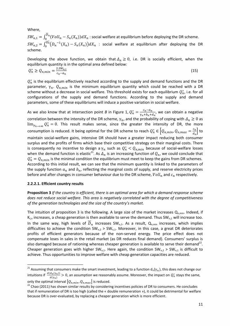
Figure 4. Maximal consumption reduction under consumers’ surplus criterion and social welfare criterion

20

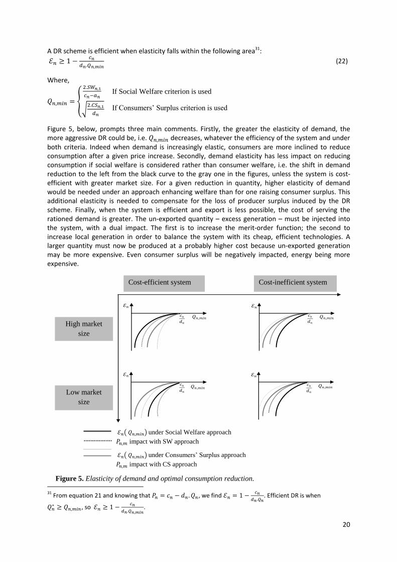
A DR scheme is efficient when elasticity falls within the following area31:

ℰ𝑛 ≥ 1 −𝑐𝑛

𝑑𝑛.𝑄𝑛,𝑚𝑖𝑛 (22)

Where,

𝑄𝑛,𝑚𝑖𝑛 =

2.𝑆𝑊𝑛,1

𝑐𝑛−𝑎𝑛

√2.𝐶𝑆𝑛,1

𝑑𝑛

Figure 5, below, prompts three main comments. Firstly, the greater the elasticity of demand, the more aggressive DR could be, i.e. 𝑄𝑛,𝑚𝑖𝑛 decreases, whatever the efficiency of the system and under both criteria. Indeed when demand is increasingly elastic, consumers are more inclined to reduce consumption after a given price increase. Secondly, demand elasticity has less impact on reducing consumption if social welfare is considered rather than consumer welfare, i.e. the shift in demand reduction to the left from the black curve to the gray one in the figures, unless the system is cost-efficient with greater market size. For a given reduction in quantity, higher elasticity of demand would be needed under an approach enhancing welfare than for one raising consumer surplus. This additional elasticity is needed to compensate for the loss of producer surplus induced by the DR scheme. Finally, when the system is efficient and export is less possible, the cost of serving the rationed demand is greater. The un-exported quantity – excess generation – must be injected into the system, with a dual impact. The first is to increase the merit-order function; the second to increase local generation in order to balance the system with its cheap, efficient technologies. A larger quantity must now be produced at a probably higher cost because un-exported generation may be more expensive. Even consumer surplus will be negatively impacted, energy being more expensive.

31

From equation 21 and knowing that 𝑃𝑛 = 𝑐𝑛 − 𝑑𝑛 . 𝑄𝑛, we find ℰ𝑛 = 1 −𝑐𝑛

𝑑𝑛.𝑄𝑛. Efficient DR is when

𝑄𝑛∗ ≥ 𝑄𝑛,𝑚𝑖𝑛 , so ℰ𝑛 ≥ 1 −

𝑐𝑛

𝑑𝑛.𝑄𝑛,𝑚𝑖𝑛.

𝑄𝑛 ,𝑚𝑖𝑛 𝑄𝑛 ,𝑚𝑖𝑛

𝑄𝑛 ,𝑚𝑖𝑛 𝑄𝑛 ,𝑚𝑖𝑛

ℰ𝑛

ℰ𝑛

ℰ𝑛

ℰ𝑛

𝑐𝑛𝑑𝑛

𝑐𝑛𝑑𝑛

𝑐𝑛𝑑𝑛

𝑐𝑛𝑑𝑛

Figure 5. Elasticity of demand and optimal consumption reduction.

If Social Welfare criterion is used

If Consumers’ Surplus criterion is used

Low market

size

High market

size

Cost-efficient system Cost-inefficient system

ℰ𝑛( 𝑄𝑛,𝑚𝑖𝑛) under Social Welfare approach

𝑃𝑛,𝑚 impact with SW approach

ℰ𝑛( 𝑄𝑛,𝑚𝑖𝑛) under Consumers’ Surplus approach

𝑃𝑛,𝑚 impact with CS approach

21

The opposite phenomenon is observed when the system is inefficient and relies massively on imports. Under the consumer-surplus approach, before the DR scheme is deployed, consumer surplus is low due to the lack of efficient generation. With the DR scheme, energy becomes more expensive than in a situation where imports are free. To cover the increased loss in their surplus due to the rising negative price effect, consumers would accept a higher cut in consumption and benefit from a more positive volume effect. Which explains why we also see a higher reduction in quantity under the consumer-surplus approach.

Results of the elasticity of demand analysis are summarized in table 3.

Table 3: Impact of elasticity of demand variation on DR program efficiency with welfare and consumer surplus scenarios

Welfare Consumer surplus

Lower DR intensity can be reached with the welfare case compared to the consumer surplus case regardless the level of elasticity of demand

Greater DR programs for high values of elasticity is possible in all scenarios for any costs level

Elasticity have less impact on DR values (unless efficient technologies and high market size)

Elasticity have more impact on DR values (unless efficient technologies and high market size)

Great elasticity of demand is needed to compensate suppliers losses

Low elasticity of demand is needed for DR to be efficient

5. CONCLUSION

This paper aims to demonstrate analytically the conditions under which activating the elasticity of consumer-demand could benefit social welfare. It supplements the literature analyzing the use of price signals to elicit demand response. Initial analysis focused on how the structure of generation technologies could affect the merit orders of countries and potential trade between them. The results show that the trade-off between producing locally and exporting energy depends on the opportunity cost of the energy and the overall efficiency of the generation technology. We have demonstrated that interconnection prices would have negative impacts on trades, regardless of their destination. This result also relies on the generation-cost differential between the interconnected systems. Indeed, if countries have significant costs differentials in generation technologies, a decrease (or increase) in imports (exports) linked with interconnection prices and exchange capacities impacts welfare and DR intensity.

Our second analysis demonstrated that there is an optimal area for the price signal, at which demand response increases social welfare. This optimality area is negatively correlated with the degree of competitiveness of the generation technologies and the market size of the system. While the literature and policy recommendations have widely highlighted that the degree of consumers’ ability to adapt their behaviour is the prime condition affecting the effectiveness of a demand response scheme, the present work has demonstrated that the impact on producer surplus must be considered as a constraint on deploying demand response. More specifically, the value of un-served energy or energy reduction the producers could lose from such a reduction in consumption would limit implementation of a scheme of this sort. Furthermore this constraint is greater if energy trade between countries is limited. However, this constraint is alleviated if the considered system in cost-inefficient as well as weakly connected with its neighbours. Our intuition was confirmed when analysis only considered the impact in terms of consumer surplus instead of social welfare. We demonstrated that under such conditions, more aggressive DR could be adopted, the weight of producer welfare being removed. Finally our analysis has demonstrated that the intensity of a demand-response scheme is negatively correlated to the degree of demand elasticity. But more elastic demand is needed if consumer surplus is the considered criteria.

22

This paper could be extended in several ways. Firstly, strategic interaction between producers, which should affect merit-order functions and consequently market equilibrium, needs to be introduced. Secondly, consumer behaviour could be more robustly analysed by integrating their satisfaction as energy consumers with a form of utility function. Consumers should also be distinguished by type and consumption profile. Bibliography Bazaraa, M.S., Sherali, H.D., Shetty, C.M., “Nonlinear Programming: Theory and Algorithm”, Wiley 2nd Edition, 1993. Bergaentzlé, C., Clastres, C., Khalfallah, H., “Demand-side management and European environmental and energy goals: An optimal complementary approach”, Energy Policy, 67, april 2014, 858-869, 2014. Boisvert R., Cappers P., Neenan B., Scott B., “Industrial and Commercial Customer Response to Real Time Electricity Prices”, Neenan Associates, 2004. Chao, H-P., “Demand response in wholesale electricity markets: the choice of customer baseline », Journal of Regulatory Economics, vol. 39, n° 1, pp. 68-88, 2011. Crampes, C., Léautier, T.O., “Demand response in adjustment markets for electricity », Journal of Regulatory Economics, vol. 48, n°2, pp. 169-193, 2015. De Jonghe C., Delarue E., Belmans R., D’haeseleer W., “Determining optimal electricity technology mix with high level of wind power penetration”, Applied Energy, 88(6), 2231-2238, 2011 (June). Di Cosmo V., Lyons, S., Nolan, A., “Estimating the Impact of Time-of-Use Pricing on Irish Electricity Demand”, The Energy Journal, 35(2), 117-135, 2014. Faruqui, A., Hledik, R., Newell, S., Pfeifenberger, H., 2007. The power of 5 Percent. Electr. J. 20 (8), 68–77. Faruqui A., Hledik R., Tsoukalis J., “The Power of Dynamic Pricing”, The Electricity Journal, 22(3), 42-56, 2009 (April). Faruqui, A., Harris, D., Hledik, R., “Unlocking the €53 billion savings from smart meters in the EU: how increasing the adoption of dynamic tariffs could make or break the EU0s smart grid investment”, Energy Policy 38 (10), 6222–6231, 2011. Faruqui, A., Sergici, S., 2010. Household response to dynamic pricing of electricity: a survey of 15 experiments. J. Regul. Econ. 38 (2), 193–225. Horowitz, S. and Lave, L., “Equity in residential Electricity Pricing”, The Energy journal, 35(2), 1-23, 2014. Kema, “Smart Grid Strategic Review: The Orkney Islands Active Network Management Scheme”, Prepared for SHEPD plc, 8th March 2012. Léautier, T.O., “The Visible Hand: Ensuring Optimal Investment in Electric Power Generation”, TSE Working Paper, n°10-153, 2012. Léautier, T.O., “Is mandating Smart Meters Smart?” The Energy Journal, 35, n°4, 135-157, 2014. Lijesen M. G., “The real-time price elasticity of electricity”, Energy Economics, 29(2), 249-258, 2007 (March). Muratori, M., Schuelke-Leech B-A., Rizzoni, G., “Role of residential demand response in modern electricity markets”, Renewable an Sustainable Energy Reviews, 33, may 2014, 546-553, 2014. Orans R., Woo C-K., Horii B., Chait M., DeBenedictis A., “Electricity Pricing for Conservation and Load Shifting”, The Electricity Journal, Volume 23, Issue 3, April 2010, pp 7-14, 2010. Park, C-K., Kim H-J., Kim Y-S., “A study factor enhancing smart grid consumer engagement”, Energy Policy, 72, September 2014. Patrick R. H., Wolak F. A., “Estimating the Customer-Level Demand for Electricity Under Real-Time Market Prices”, NBER Working Paper N°8213, 2001 (April). Strbac G., “Demand side management: benefits and Challenges”, Energy Policy, 36:12: 4419-4426, 2008. Stoft, S., “Power System Economics: Designing Markets for Electricity”, IEEE Press, Piscataway, 2002.

23

Ventosa N., Baillo A., Ramos A., Rivier M., “Electricity market modeling trends”, Energy Policy, 33( 7), 897-913, 2005 (May). Vespucci M.T., Innorta M., Cervigni G., “A Mixed Integer Linear Programming model of a zonal electricity market with a dominant producer”, Energy Economics, vol. 35, pp 35-41, 2013. Woo C-K., “ Efficient Electricity Pricing with Self-Rationing”, Journal of Regulatory Economics, vol. 2, n° 1, pp. 69-81, 1990.

APPENDIX

Appendix 1:

On the assumption that the merit-order function is an aggregation of the individual marginal costs of

available technologies, we define 𝑃𝑡,𝑛(𝑥𝑡,𝑛) = 𝑎𝑡,𝑛 + 𝑏𝑡,𝑛. 𝑥𝑡,𝑛 as the individual inverse-supply

function of a given technology in a given country. Therefore 𝑥𝑡,𝑛(𝑃𝑡,𝑛) =𝑃𝑡,𝑛−𝑎𝑡,𝑛

𝑏𝑡,𝑛 is the individual

supply function.

When the market is cleared, all market participants receive the same electricity price, hence 𝑃𝑡,𝑛 = 𝑃𝑛

∗ for all technologies producing in country n, i.e. both the price of local technologies and exporters are considered. By aggregating all the individual supply functions, the aggregated function at equilibrium will take this form (equation (2) in section 2):

𝑃𝑛∗ = 𝑎𝑛 + 𝑏𝑛𝑋𝑛

If we now replace 𝑋𝑛 by the sum of the quantities of all generation technologies potentially producing in country n (including imports from the other country), and simplify the equation above, we find the parameters of the aggregated inverse-supply function as follows:

𝑎𝑛 =∑ 𝑎𝑡,.𝑏,+∑ 𝑎𝑡,.𝑏,+∑ 𝑎𝑡,.𝑏𝑡,𝑡,𝑡,𝑡,

∑ 𝑏𝑡,𝑡, and 𝑏𝑛 =

∏ 𝑏𝑡,𝑡,

∑ 𝑏𝑡,𝑡,

Where, is the index of the country selling electricity in country n, is the index of the technologies different from technology t and is the index the other country selling electricity in country n.

Appendix 2:

We state our equilibrium model as a Mixed Complementarity Problem by first determining the first-order optimality conditions associated with each country’s scheme. To calculate the optimality conditions for each scheme, we define the Lagrangien function of the corresponding optimization

problem, 𝐿𝑎𝑔𝑛 :

𝐿𝑎𝑔𝑛 = ∑ [𝑋𝑡,𝑛. (𝑎𝑡,𝑛 +1

2. 𝑏𝑡,𝑛. 𝑋𝑡,𝑛)]𝑡 − 𝑟𝑡,𝑛. (𝐾𝑡,𝑛 − 𝑋𝑡,𝑛) − 𝑃𝑛,𝑚. (𝐶𝑎𝑝𝑛,𝑚 − ∑ 𝑥𝑡,𝑛,𝑚𝑚 ) −

𝑓𝑛. (𝐿𝑛 − ∑ 𝑥𝑡,𝑛 − ∑ ∑ 𝑥𝑡,𝑚,𝑛𝑚𝑡𝑡 ) Then we calculate the gradient of the Lagrangian function with respect to each decision variable: 𝑑𝐿𝑎𝑔𝑛

𝑑𝑥𝑡,𝑛 and

𝑑𝐿𝑎𝑔𝑛

𝑑𝑥𝑡,𝑛,𝑚

The optimality conditions of each scheme are:

0 ≤𝑑𝐿𝑎𝑔𝑛

𝑑𝑥𝑡,𝑛 ⊥ 𝑥𝑡,𝑛 ≥ 0

0 ≤𝑑𝐿𝑎𝑔𝑛

𝑑𝑥𝑡,𝑛,𝑚 ⊥ 𝑥𝑡,𝑛,𝑚 ≥ 0

0 ≤ (𝐾𝑡,𝑛 − 𝑋𝑡,𝑛) ⊥ 𝑟𝑡,𝑛 ≥ 0

24

0 ≤ (𝐶𝑎𝑝𝑛,𝑚 −∑ 𝑥𝑡,𝑛,𝑚𝑚 ) ⊥ 𝑃𝑛,𝑚 ≥ 0

𝐿𝑛 − ∑ 𝑥𝑡,𝑛 − ∑ ∑ 𝑥𝑡,𝑚,𝑛𝑚𝑡𝑡 = 0 𝑓𝑛 𝑓𝑟𝑒𝑒

Grouping together the optimality constraints of the two schemes leads to an MCP problem. Since the cost functions are convex and continuously differentiable, the KKT conditions are necessary and sufficient for the existence and the uniqueness of the solution (Bazaraa et al. (1993)). The solution 𝑥

is unique and simultaneously satisfies the above constraints: 𝑥 =

(

𝑥𝑡,𝑛∗ ∀𝑡, 𝑛

𝑥𝑡,𝑛,𝑚∗ ∀𝑡, 𝑛

𝑟𝑡,𝑛∗ ∀𝑡, 𝑛

𝑃𝑡,𝑛∗ ∀𝑡, 𝑛

𝑓𝑛∗ ∀𝑛 )

Appendix 3:

By developing the above program in Appendix 3, we obtain the following equations:

𝑎𝑡,𝑛 + 𝑏𝑡,𝑛. 𝑥𝑡,𝑛 = −𝑟𝑡,𝑛 − 𝑓𝑛

𝑎𝑡,𝑛 + 𝑏𝑡,𝑛. 𝑥𝑡,𝑛,𝑚 = −𝑟𝑡,𝑛 − 𝑃𝑛,𝑚 − 𝑓𝑚

Subtracting the above equations and replacing 𝑏𝑡,𝑛 by 𝛼𝑡−1. 𝑏, we can verify that: 𝑥𝑡,𝑛 = 𝑥𝑡,𝑛,𝑚 +𝑓𝑚−𝑓𝑛+𝑃𝑛,𝑚

𝛼𝑡−1.𝑏1 .

Replacing 𝑥𝑡,𝑛,𝑚 by 𝑥𝑡,𝑛 −𝑓𝑚−𝑓𝑛

𝛼𝑡−1.𝑏 as determined above. We find:

∑ 𝑥𝑡,𝑛 + ∑ 𝑥𝑡,𝑚 − ∑

𝑓𝑛−𝑓𝑚+𝑃𝑛,𝑚

𝑏𝑡,𝑚𝑡𝑡𝑡 = 𝑄𝑛

∑ 𝑥𝑡,𝑚 + ∑ 𝑥𝑡,𝑛 − ∑𝑓𝑚−𝑓𝑛+𝑃𝑚,𝑛

𝑏𝑡,𝑛𝑡𝑡𝑡 = 𝑄𝑚

We find that: 𝑓𝑚 − 𝑓𝑛 =𝑏1.(𝐿𝑛−𝐿𝑚)

∑ 1

𝛼𝑡−1𝑡,𝑛

+𝑃𝑚,𝑛.∑

1

α𝑡,𝑚𝑡

∑ 1

𝛼𝑡−1𝑡,𝑛

−𝑃𝑛,𝑚.∑

1

α𝑡,𝑛𝑡

∑ 1

𝛼𝑡−1𝑡,𝑛

and𝑥∗𝑡,𝑛 − 𝑥∗𝑡,𝑛,𝑚 =

𝑄𝑛−𝑄𝑚𝛼𝑡−1

𝛼−1

+

(1−𝛼).∑ 𝑃𝑛,𝑚𝑛

𝛼𝑡−1.(1−𝛼𝑡).𝑏. ∑

1

𝛼𝑚𝑡−1𝑡

Appendix 4:

System operators would prefer less costly technologies to balance their systems. We assume first that ∑ 𝐾𝑡,𝑛𝑡,𝑛 ≥ ∑ 𝑄𝑛𝑛 , 𝐾𝑡,𝑛 ≤ ∑ 𝑄𝑛𝑛 .

Secondly, we assume that technology t in country n is the most efficient. Therefore: 𝑥𝑡,𝑛 + 𝑥𝑡,𝑛,𝑚 =

𝐾𝑡,𝑛. Hence, from equation 9b, 𝑥∗𝑡,𝑛 =𝐾𝑡,𝑛

2+𝑄𝑛−𝑄𝑚

2.𝜔𝑡+∑ 𝑃𝑛,𝑚𝑛 .∑

1

α𝑡,𝑚𝑡

𝑏.𝜔𝑡 and 𝑥∗𝑡,𝑛,𝑚 =

𝐾𝑡,𝑛

2−𝑄𝑛−𝑄𝑚

2.𝜔𝑡−

∑ 𝑃𝑛,𝑚𝑛 .∑1

α𝑡,𝑚𝑡

𝑏.𝜔𝑡 .

For an inefficient technology, we may assume that, if called to produce, the total quantity fed into

both markets would not reach the capacity of the technology. We assume 𝑡 to be the index of the

inefficient technology. In this case, 𝑟𝑡,𝑛 = 0, because the capacity constraint is not saturated. For ∀ 𝑡

and from 𝑑𝐿𝑎𝑔𝑛

𝑑𝑥𝑡,𝑛= 0 and

𝑑𝐿𝑎𝑔𝑛

𝑑𝑥𝑡,𝑛,𝑚=0, we find that:

𝑥𝑡,𝑛 =𝑎,𝑛−𝑎𝑡,𝑛

𝛼𝑡−1.𝑏1+𝛼−1

𝛼𝑡−1. 𝑥𝑡,𝑛 , ∀ 𝑡 and 𝑥𝑡,𝑛 =

𝑎,𝑛−𝑎𝑡,𝑛

𝛼𝑡−1.𝑏1+𝛼−1

𝛼𝑡−1. 𝑥𝑡,𝑚,𝑛 +

𝑃𝑚,𝑛

𝛼𝑡−1.𝑏1 , ∀ 𝑡

25

Given that at equilibrium 𝑄𝑛 = ∑ 𝑥𝑡,𝑛 + ∑ ∑ 𝑥𝑡,𝑚,𝑛𝑚𝑡𝑡 , and replacing 𝑥𝑡,𝑛 and 𝑥𝑡,𝑚,𝑛 by their

respective terms, we find that: 𝑥∗𝑡,𝑛 =𝑅𝑒𝑠𝑛−ɸ𝑡𝜔𝑡

+𝑃𝑚,𝑛

𝑏.𝜔𝑡. ∑

1

α𝑡,𝑚𝑡 and 𝑥∗𝑡,𝑛,𝑚 =

𝑅𝑒𝑠𝑚−ɸ𝑡𝜔𝑡

−𝑃𝑛,𝑚

𝑏.𝜔𝑡. ∑

1

α𝑡,𝑚𝑡 .

We note that if all the technologies are inefficient, ∑ 𝑥∗𝑡,𝑛,𝑚𝑡 = ∑ 𝑥∗𝑡,𝑛𝑡 = 0 in the above equations.

Of course these solutions 𝑥 =

(

𝑥∗𝑡,𝑛 ∀𝑡, 𝑛

𝑥∗𝑡,𝑛,𝑚 ∀𝑡, 𝑛

𝑥∗𝑡,𝑛 ∀𝑡, 𝑛

𝑥∗𝑡,𝑛,𝑚 ∀𝑡, 𝑛)

only hold if 𝑥 ≥ 0 and the sum of local generation

and exports for a given technology does not exceed its available capacity.