Embed Size (px)
Citation preview

Alexander John Finch Page 1 MSc in Automotive Engineering
Submitted by Alexander John Finch
For the degree of MSc in Automotive Engineering
Department of Mechanical Engineering
University of Bath
September 2001
COPYRIGHT
Attention is drawn to the fact that copyright of this dissertation rests
with the author. This copy of the dissertation has been supplied on
condition that anyone who consults it is understood to recognise that its
copyright rests with its author and that no quotation from this
dissertation and no information derived from it may be published without
the prior written consent of the author.
This dissertation may be available for consultation within the University
Library and may be photocopied or lent to other libraries for the purpose
of consultation.
Alexander John Finch …………………………….
An Application of Bayesian
Statistics to Engine
Modelling.

Alexander John Finch Page 2 MSc in Automotive Engineering
Abstract
This report explores the possibility of reducing the calibration time of spark ignition engines using mathematical modelling and prior knowledge based Bayesian statistical methods. Second order models are used to analyse the effect on a single response variable of one or two input variables. Bayesian statistical techniques allow a mathematical model of engine data to be updated with each additional data point and as such used as a tool with which to assess the current model. This includes convergence criteria based on the coefficients of the current model, confidence intervals for the current model and predictive intervals for a single future observation. The effect of prior knowledge on these assessment tools is explored, looking particularly at the differences in convergence time between good and poor prior knowledge of the model coefficients. Methods for selecting data are also explored, looking particularly at the effect various different proposed techniques have on the convergence time.
Acknowledg ements
Thanks to Dr Christian Brace for supervision of the project.
Thanks to Dr Gavin Shaddick for his assistance with problems of a mathematical nature.
Contents
1. Background.
1.1 Introduction. Page 1
1.11 Experimental Design
1.12 Bayesian Statistics.
1.13 The Likelihood.
1.14 Bayes Theorem.
1.2 Literature Review. Page 4
1.21 Review of Reference [1].
1.22 Review of Reference [2].
1.23 Review of Reference [3].
1.24 Review of Reference [4].
1.25 Conclusions.
1.3 Aims. Page 11
1.4 Objectives. Page 11
1.5 Implementing the Bayesian Method. Page 12
1.6 Linear Models Page 14
1.61 Least squares model fitting.
1.62 Estimating the Variance.

Alexander John Finch Page 3 MSc in Automotive Engineering
1.63 The Variance/Covariance matrix
1.64 Modelling Engine Data
2. Programming the Bayesian method.
2.1. MATLAB Program Details. Page 19
2.2 Demonstration of prior knowledge on convergence . Page 20
2.21 Quadratic functions.
2.22 Cubic functions.
3. Model Convergence
3.1 Convergence Criteria. Page 28
3.2 Effect of prior knowledge on convergence times. Page 32
3.21 Convergence to Quadratic functions.
3.22 Simulating errors.
3.23 Convergence to Quadratic functions with
simulated errors.
3.24 Convergence to Cubic functions.
3.24 Convergence to Cubic functions with
simulated errors.
3.25 Convergence of engine data to second order
Taylor approximation.
3.27 Conclusions.
4. Model Assessment
4.1 Confidence Intervals. (C.I.’s) Page 47
4.11 What are Confidence Intervals?
4.12 How to calculate C.I.’s.
4.13 Effect of prior knowledge on C.I.’s using functions
as datasets. One variable.
4.14 Effect of model variance on C.I.’s. One variable.
4.15 Effect of prior knowledge on C.I.’s using functions
as datasets. Two variables.
4.16 Effect of model variance on C.I.’s. Two variables.
4.17 C.I.’s using engine-testing data.
4.18 Conclusions.
4.2 Predictive intervals. Page 60
4.21 What are predictive intervals?
4.22 How to calculate P.I.’s.
4.23 Effect of prior knowledge on P.I.’s using functions
as datasets. One variable.

Alexander John Finch Page 4 MSc in Automotive Engineering
4.24 Effect of model variance on P.I.’s. One variable.
4.25 Effect of prior knowledge on P.I.’s using functions
as datasets. Two variables.
4.26 Effect of model variance on P.I.’s. Two variables.
4.27 P.I.’s using engine-testing data.
4.28 Conclusions.
5. Scaling the Input Variables Page 72
6. Testpoint Selection Methods.
6.1 Why select testpoints? Page 75
6.2 Selection procedures. Page 76
6.3 Convergence comparisons. Page 77
6.31 One variable.
6.31 Two variabes.
6.4 Conclusions. Page 86
7. Conclusions
7.1 Convergence. Page 87
7.2 Confidence Intervals. Page 88
7.3 Predictive Intervals. Page 89
7.4 Overall. Page 89
8. Recommendations Page 92
8.1 Second Order Bayesian Models. 8.2 Future Work.
9. References Page 93
10. Appendices Appendix I MATLAB program details Page 94
Appendix II Residual plots Page 97
Appendix III Hypothesis testing Page 100

Alexander John Finch Page 5 MSc in Automotive Engineering
1. Background.
1.1 Introduction
Traditionally engine design and development has been characterised by beginning with a wide
range of possible options which are subsequently tested via many levels of analysis, i.e. broken
down into sub-processes, whereby decisions are made on the likely optimum settings in the
light of previous experience. These tests normally take the form of repeated, comparative
analysis of each configuration against the current benchmark.
Statistical techniques offer greater benefits as engine hardware variables increase in both
number and complexity and the collection of data becomes more difficult. It is no longer the
case that an engineer can intuitively know how changing a particular set of variables will affect
the performance characteristics of a given engine. The benefits of combining different
technologies are decreasing at the same time making it difficult to assess the effect. Advances
in on-board electronics, and ECU’s now standard automobile hardware, mean that much more
information is available for the modelling process. This makes individual decisions far more
critical as their consequences can be far reaching into areas which have not even been
reasoned for.
The overall aim is to be able to design and test a wider range of possible options in the same
time & cost but with increased confidence in the results by more accurately quantifying the
effects and uncertainties.
Engine development is essentially driven by three factors;
1. lower cost engines
2. reduced exhaust emissions
3. increases in vehicle performance & refinement
1.11 Experimental Design
“By the statistical design of experiments, we refer to the process of planning the experiment so
that appropriate data that can be analysed by statistical methods will be collected, resulting in
valid and objective conclusions.” [5]
Experimental design was originally developed in the agricultural industry and then adopted by
the chemical industry until it was popularised by Taguchi and is now well documented through
concurrent engineering concepts and methods.

Alexander John Finch Page 6 MSc in Automotive Engineering
There are essentially two aspects to any experiment - design of the experiment and analysis of
the data. These are obviously related since the type of analysis depends on the experimental
design.
The three basic principles of experimental design -
1. REPLICATION - allows us to estimate the experimental error (variance) and gives more
precise estimates of population parameters.
2. RANDOMISATION - the order in which trials are undertaken is determined randomly.
Statistical methods require experimental error to be independently distributed random
variables. Randomisation usually makes this valid. It also helps to average out
inconsistencies in the experimental design.
3. BLOCKING - used to increase experimental precision. A given block should be more
homogeneous than the entire experimental set. Each block is tested in turn in a
randomised order.
Design of Experiments (DoE) methodology gives us the following-
� Increased information from a given series of tests, including the relative contributions of
different variables - normally realised as weighted model parameters.
� An opportunity to make inferences about optimum settings and to be able to produce
confidence limits to describe the likelihood of the estimates.
� Reduction in testing time and cost. Through less testing or better planning and execution of
experiments.
Despite these clear advantages application of DoE to engine development processes has been
relatively limited.
Due to the complexity of increased variables the “one factor at a time” approach has typically
been used. All the variables except one are fixed making the model much simpler to analyse.
This simplicity fails to give us any information about how the system reacts when a combination
of variables is changed and is therefore becoming less useful as an analysis tool.
1.12 Bayesian Statistics
Bayesian statistics is a different approach to the conventional theory, which is frequentist
statistics.
Any problems in statistics can be tackled either by the frequentist or the Bayesian approach.
Comparison between Bayesian and frequentist approaches:-

Alexander John Finch Page 7 MSc in Automotive Engineering
�� Bayesian Statistics uses prior information, which represents all that is known in addition to
the data. Frequentist statistics does not, and so makes less use of the available
information. Consequently a Bayesian analysis can often come to stronger conclusions
than a frequentist analysis of the same data.
�� Frequentist statisticians object to the use of prior information because it is subjective,
depending on the personal judgement of the individual from whom the information is
elicited.
�� Frequentist inference procedures are derived from the likelihood p(y/�), and are based on
treating � as fixed but unknown. Bayesian inferences are derived from the posterior
distribution p(�/y), and treat the observed data as known and therefore fixed.
� In frequentist statistics the parameters are never random variables. In Bayesian statistics
anything unknown is random.
� There are cases where only a Bayesian approach can give an answer, when the problem is
far too complex for a frequentist solution to be found.
1.13 The Likelihood
Suppose we observe the data xi i = 1, …. ,n with associated responses yi.
We assume a model Pr(Yi = yi) = f(yi / xi, �) where � is a vector of unknown model parameters.
Then assuming that the yi’s are independent the probability of observing the values y1, …., yn is,
��
n
i 1
f(yi / xi, �), (�).
Considered as a function of � (�) is called the likelihood for � written L(� ; y1, …., yn, x1, …., xn ) or
L(� ; y).
Example. Suppose we assume the model Pr( Yi = yi ) = � � exp {-��yi}.
Then L(� ; y) = ��
n
i 1
� � exp {-� � yi},
= �n � exp {-� � �
�
n
i 1
yi },
We can then use this likelihood to estimate � by finding the value of � that maximises L( � ; y ).
Alexander John Finch Page 8 MSc in Automotive Engineering
N.B. If � maximises L( � ; y ) then � also maximises log L( � ; y ) from standard calculus
methods.
log L( � ; y ) = n � log � - ����
n
i 1
yi
( d / d� ) log L = n / � - ��
n
i 1
yi
( d / d� ) log L = 0 when � = n / ��
n
i 1
yi .
So that the maximum likelihood estimator is the inverse of the sample mean.
1.14 Bayes Theorem
p( � / y ) = p( � )�p( y / � ) where p( y ) = � p( � )�p( y / � ) d� is a constant.
p( y )
Hence the posterior distribution, p( � / y ), is dependent upon the prior, p( � ), and on the
likelihood, p( y / � ).
In fact since p( y ) is a constant the following simple relationship applies:-
p( � / y ) � p( � )�p( y / � ) or posterior � prior � likelihood
There is a group of prior distributions that, given the likelihood, give rise to a posterior
distribution of the same form as the likelihood. These are known as conjugate priors. The
ability to recognise the form of the posterior enables the normalising constant to be inferred,
since � p( � ) d� = 1. This saves time performing integration, both analytical and numerical.
1.2 Literature Review
1.21 Review of Reference [1]. This paper was written by a team from Ricardo Consulting
Engineers and was the main presentation in the IMechE journal entitled, ‘Statistics for Engine
Optimisation’, which incidentally was sponsored by Ricardo. The authors take us through the
history of the engine development process - such as how it wasn’t until the 1980’s when
sufficient computing power was available to implement statistical techniques effectively - and
then go on to describe the direction the future of engine development should be headed.
There is a distinct theme running through this paper. It is geared towards Bayesian statistical
methodology. There are various references throughout to the need for prior information such as
-

Alexander John Finch Page 9 MSc in Automotive Engineering
“We need to make more use of the data from any individual exercise: we need to be able to
manage our database more effectively and use it to answer conjectures in relation to future
potential products.”
“The use of prior knowledge in order to estimate the likely consequence of parameter
combinations and hence check the ‘runnability’, increased significantly as the experience grew.”
“...so on-line checking of the experimental data could be implemented. Outlying data could be
identified and the test repeated or weighted accordingly.”
“...benefit from prior knowledge of both the engine behaviour and realistic measurement
uncertainties.”
“Finally, it would be helpful if there was a formal method for including engineering knowledge
before a statistical experimental programme was undertaken: this would also help to improve
the communication between the statistician and the engineer.”
It then goes on to describe the benefits of Bayesian experimental Design and papers Ricardo
have already published on the subject, references [3] and [4]. These are in fact almost the only
papers published on the subject making it rather in the interests of Ricardo to present the case
for Bayesian methodology.
Traditionally the use of empirical models has been restricted to 2nd order polynomials as they
give a good compromise in terms of flexibility and computational efficiency. However these
have been found to be inappropriate in many cases and there has been a move into the use of
non-linear and stochastic process models. This is particularly true when trying to model
particulate matter. “Very early in the application of statistical design of experimental techniques
it became clear that , for certain purposes, 2nd order models were inadequate.” Instead higher
order models were tested for ‘lack of fit’ so that, given the data, the simplest model that
captured the main trends could be used.
There has also been progress made into the automation of testing, whereby it is possible to run
tests overnight on software variables and a re-build undertaken the following day. This is likely
to lead to major reductions in overall testing time and can also deliver a greater number of test
points enabling a clearer picture of an engines characteristics to be understood. There are
several pointers towards the use of Bayesian statistics in an automated capacity. “..potential for
automation, through the use of prior based designs and model parameters.”
In engine research the optimisation is always constrained meaning that the process of
optimisation is not purely mathematical but involves making compromises between the
variables. As more engine build decisions are taken the list of constraints and requirements
increases. Empirical models and optimisation techniques need to be flexible enough to work
with badly behaved response surfaces. Such techniques though are often extremely computer
intensive and as such developments in Genetic Algorithms and Neural Networks are being
explored.

Alexander John Finch Page 10 MSc in Automotive Engineering
With respect to measurement uncertainty it has been noted that components that are re-built to
exactly the same specification can give statistically significant differences in engine
performance. It is therefore desirable to keep the number of engine re-builds to a minimum.
In describing a route for the future they go to say that, “essentially, development is experienced
based engineering therefore it is inherently Bayesian”. They would like to see statistics as an
integral part of the development process. A consistent method of storing prior models from
research and from previous vehicle builds so that a Bayesian environment is effectively
introduced which would almost be a re-engineering of current practices.
Whilst there are clear benefits to be gained from a Bayesian approach it is not the only available
tool and neither is it necessarily the most effective.
1.22 Review of Reference [2] =. Gives us a general idea of some of the practical implications
of statistical engine testing. Engine optimisation always involves trade-offs between the various
variables and so during calibration we tend to search for a constrained optimum. i.e. to find the
“engine set up which minimises fuel consumption (BSFC) and noise while meeting the EURO III
emission limits and attaining an acceptable max. in cylinder pressure.” It is also suggested that
when designing an empirical model, “the design should enable the relationships between the
responses (or some transformation of them) and the six parameters to be modelled using a 2nd
order Taylor series approximation.” This is presumably for similar reasons to those given in
reference [1].
Although they have chosen to design around a 2nd order model, “it was noted that the presence
of a 3rd order interaction term meant that extrapolating at the extreme hardware settings was
unwise, but interpolation gave rise to meaningful results.” We therefore need to design the
range our experiment to encompass the greatest range of data we are likely to use, if a 2nd
order model is to be implemented. Although this also means that we may not be capturing all
the information we would ideally like.
It is also stated that, “for ease of communication, the engineer should be able to use some of
the data collected to plot the traditional one-factor-at-a-time influence diagrams
(response/factor)”. This makes sense since it is almost impossible to imagine how varying more
than two factors at a time will affect the response.
From the fitted model a 95% prediction interval was constructed. This is the interval for which
we are 95% certain that future observations will lie. “Since all the data fell within the 95%
prediction interval we could consider this model to represent the engine behaviour accurately.”
This means that there were no outliers given the fitted model. Although, the fact that all the
data fell within the 95% prediction interval does not necessarily mean that the model is
accurate. It would be perfectly possible to construct a model for which this held and for which

Alexander John Finch Page 11 MSc in Automotive Engineering
the model did not capture the engines behaviour accurately. The predictive interval is merely
an expression of both the variability of the model coefficients and the variability in the data.
Hence large variabilities lead to large intervals which contain the data.
They go on to comment, “it is often the case that, a trade-off must often be made between
statistical considerations, such as randomisation, blocking and engineering requirements such
is the desire to keep the number of rebuilds to a minimum.” This is in agreement with reference
[1]. In our study though we are not so much concerned with re-builds as quicker and more
efficient calibration is the main objective.
They state the aims of statistical engine testing as –
�� Reduction in testing time / more efficient use of the time available
�� Information about the most influential parameters and their interactions
�� Confidence in the results
�� Flexible data structure
Again this agrees with reference [1].
All these 2nd order models come from different applications but the basic idea is to be able to
capture some degree of curvature and interaction between different parameters whilst keeping
the model as simple as possible. This is usually the ideal case. It has been noted that the 2nd
order model does have its limitations, such as its inability to capture some of the more subtle
interactions you might find when modelling particulate matter. Although parameter transforms
can go some way to solving this problem. Even a 2nd order model, if we consider the effect of
three variables on a response, can contain up to as many as ten terms. If we wanted to model
eight input variables then we would have to account for up to 45 terms which is starting to get
far too complex to be of much practical use, especially when it comes to interpretation using
traditional regression techniques. A model with 45 terms would also require at least 45 test
points before any classical statistical analysis could be undertaken.
1.23 Review of Reference [3] .
Many of the same arguments from reference [1] are given here. The introduction talks about
how it is “unfeasible to test all the possible combinations of settings.” Referring to the trade-offs
between the experimental variables when searching for an optimum solution. There is also
some comment about the random ‘noise’ that is always present that causes differences in
results when tests are repeated.
The drawbacks of the traditional approach are highlighted - how the approach of varying one
factor at a time is, “unlikely to lead to a general understanding of the underlying trends and may
fail to produce robust operating strategies due to the presence of unsuspected interactions or
sensitivities.”

Alexander John Finch Page 12 MSc in Automotive Engineering
They describe the problem of being unable to, “fit a model until the full test matrix is completed”
and how “this lack of feedback during the course of testing is generally unsatisfactory for those
responsible for the management of the project.” Although this sounds more like it would be an
advantage to be able to provide feedback rather than it hinders project management to be
without it.
They go on to say how it is not possible to “use the initial results to alter the test programme in
order to concentrate effort on parts of the design region which are most likely to be of interest in
subsequent optimisation”, and that, “prior engineering knowledge of the likely behaviour of the
engine is not fully exploited.” Again this sounds like it has been written after the advantages of
using this particular technique had been verified simply to highlight its benefits.
Bayesian statistical methodology is described briefly. The basic idea is that you can describe
your prior beliefs about a system using probability distributions to explicitly model unknown
parameters. A distribution is assumed for the test data, used to create the likelihood function,
which is then combined with the prior distribution to produce an overall belief function called the
posterior distribution. The advantage is that before any testing has taken place a functioning
model is already available. As data is collected the posterior is updated. If the prior model is an
accurate description of the system then the model should converge quickly given few test
points. If the prior is a poor description of the system then given sufficient test data its influence
can be overcome. This gives the advantages described previously.
As a staring point it is suggested that a 2nd order Taylor approximation is used. They seem to
think that this model will be useful for providing information about spark sweeps and their effect
on variables such as ignition delay, exhaust temperature, CO, NOx , thermal efficiency, burn
rate, max cylinder pressure etc. It is also suggested that the Taylor approximation would be of
more use when initially mapping over the whole range of parameters to get a feel for how the
system behaves. Once an area of interest has been identified the model could be applied to a
smaller region to give a better approximation or a more elaborate model employed.
“More fundamentally based models are required to help explain the mechanisms relating the
input parameters (injection timing, injection rate, etc.) to the responses.” But, as we have heard
previously the 2nd order Taylor approximation is used frequently for such purposes.
They have developed a package that allows engineers to graphically describe their beliefs
about the relationships between variables and responses. The engineer is asked to draw the
curve that best represents their beliefs about the system and then asked to give a 95%
confidence interval for those beliefs. The graphs created are then translated into model
coefficients and the variance can be inferred from the confidence intervals. Whilst this method
is of use during a new experimental programme, generally the prior beliefs can be entered
directly as empirical models from other engines or stages of the test programme. For instance if

Alexander John Finch Page 13 MSc in Automotive Engineering
an engine has already been thoroughly mapped it makes sense to fit a model to it and then use
that as a prior distribution for subsequent alterations or even re-builds.
Another benefit of the Bayesian approach is that, “before a set of tests are performed, prediction
intervals can be computed for the expected responses.” Any subsequent data that falls outside
this reason can be treated as suspect - there might be a problem with the measurement of
results and the test repeated, or the data point may simply be an outlier and could be weighted
accordingly.
We have seen previously how variable selection can pose a problem when specifying the
model. Too few terms and the model is a poor fit to the data, too many and the model may fit
noise into the system. The Bayesian approach offers a way around this. All variables can be
included but if it is thought that they may be less important they can be assigned tight prior
distributions around zero. They only subsequently become important if sufficient data is
available to establish a need.
1.24 Review of Reference [4] .
This paper compares the Bayesian techniques described in reference [3] with the classical
methods. Prior information is supplied by two engineers with different backgrounds and
experience. An engine which has been thoroughly mapped previously is used to create the
“true” reference model.
They begin by making the observation that there are philosophical objections to be made about
introducing a subjective element into the engine testing procedure by modelling prior
knowledge. As long as the prior knowledge is based on all the currently available data this
should not be a problem.
The graphical technique of eliciting prior information from the engineers is used. “Both
engineers found it relatively easy to produce estimates of the mean curves using the graphical
interface, but found the concept of defining confidence limits for their estimates more difficult.”
This is partly due to the unfamiliarity of most engineers with statistical techniques. The
confidence limits were used to ascertain the variability of the mean curves.
Engineer A chose to define more interaction terms and showed reasonable confidence in his
estimates. Engineer B specified wider confidence limits. This meant that initially, prediction
intervals for engineer B were larger since he had inferred a greater model variance.
“In general, a reasonably accurate prior distribution converged well to the “reference” model
and was good at detecting outliers.”

Alexander John Finch Page 14 MSc in Automotive Engineering
In fact even if the coefficients were poorly specified but a large variance was used , then the
model still converged well given only a small amount of data. This has the effect of making the
prediction intervals wider and as such outlier detection is limited.
As testing continues the confidence intervals should decrease. An example given is one of
minimising BSFC subject to BSNOx being below 7 g/KWh. Plotting the model with a 95%
confidence limit it can be seen that if the mean of the distribution is used then the point at which
this is satisfied is a1. However due the imprecise estimates of the model parameters we might
choose to take the estimate a2 causing a subsequent increase in fuel consumption. Since the
confidence intervals will decrease as more data is collected the “penalty” for choosing a2 over
a1 will decrease. This “penalty” can be used as a method of selecting future test points as well
as a stopping criteria. See figure 1.2a
Problems with the prior distribution arise when the parameter values are not accurately
specified and the variance is low. In this case the posterior is slow to converge.
As a comparison, after 17 tests both models provided a good approximation of the “true” model,
which was generated using 131 tests. This represents a substantial saving in test time.
However, although 131 tests were used to generate the model, could it have been achieved
with less?
1.25 Conclusions
Overall it is clear that the Bayesian Method has many advantages when it comes to engine
testing.
Advantages:
�� Potential for automation of test-rigs.
�� Opportunity to alter the test program as new information becomes available.
Figure 1.2a

Alexander John Finch Page 15 MSc in Automotive Engineering
�� An ability to overcome the problem of variable selection. Too few and the model is a poor
fit. Too many and it is possible to capture a lot of random noise.
�� A reduction in the calibration time.
�� The ability to identify suspect data as they are recorded as well as possible faults with the
measuring equipment.
�� Convergence criteria – to enable automation.
�� Flexibility in the model. Allows us to drop terms if they become less significant in light of the
data.
Disadvantages
�� More complicated to implement if a non-conjugate prior is selected. (need numerical
integration techniques)
�� Choice of prior is subjective.
�� Poor prior information can lead to an increase in the number of test points required and
hence an increase in the engine calibration time.
Bayesian statistics can be applied to the same problems as classical statistics. The problem of
being restricted only to conjugate priors has been largely overcome due to increases in
numerical multi-dimensional integration techniques and computing power.
1.3 Aims
To use Bayesian statistical techniques to reduce the calibration time of a spark ignition engine
and as a device to guide the direction of testing and create more robust engine models.
1.4 Objectives
Develop a Bayesian engine modelling program in MATLAB.
Develop convergence criteria for the model as it is updated to enable automation to be realised.
Analyse the effect of varying prior knowledge on the convergence time and robustness of
second order engine models.

Alexander John Finch Page 16 MSc in Automotive Engineering
1.5 Implementing the Bayesian Method
The following flow diagram illustrates the main points of the Bayesian Method.
1. Assume a general model for the parameters considered.
�
2. Apply prior knowledge to the
parameters to form the prior
distribution, p( �� ).
Either from previous data on
similar engines or with estimates
elicited from engineers.
�
3. Carry out initial testing.
Form likelihood, p( y / �� ).
�
4. Update the model parameters.
p( �� / y ) � p( �� )�p( y / �� )
�
� �
5. Test for significance of model parameters to simplify model. �
� �
6. Decide where to test next. �
� �
7. Combine new test point with original data to form new likelihood.
Test model for convergence.
1. Modelling will be implemented using a special case of the general linear model y = X�� + �
where �� is a ( kx1) vector of coefficients, � is the error term which is assumed to follow a
normal distribution, � ~ N ( 0, �2I ) and X is an (nxk) matrix containing all the various
combinations of parameters that make up the model. For a 2nd order model these include
the constant, linear, quadratic and interaction terms.
2. The prior p( �� ) will be formed from modelling data from similar engines. Assuming that the
coefficients are independently normally distributed, �� ~ N ( ��0, �2 ��0 ).
3. Assuming that the data comes from a normal distribution the likelihood takes the following
form; p( y / �� ) � exp { -1/( 2�2) ( y - X�� )T( y - X�� ) }.

Alexander John Finch Page 17 MSc in Automotive Engineering
4. It follows that the posterior distribution is normally distributed.
�� / y ~ Nk [ (��0 -1 + XTX )-1( XTy + ��0
-1��
0 ), �2 (��0 -1 + XTX )-1 ].
5. Parameters whose values are converging to zero have less and less weighting on the
model structure and can therefore be ignored. This information can be noted for use in
future testing. Note that the magnitude of the input variables needs consideration here –
see section 5.
6. It is possible to select new testpoints dependent on some pre determined criteria i.e. maybe
in light of the current model we wish to test in a particular data area. It is important to note
that the model is based on the assumption that the data comes from a normal distribution
and that it is random. By formally selecting each test point we invalidate this assumption
and many of the analysis tools become much less useful. However it may still be possible
to maintain a degree of randomness within a structure using techniques such as blocking.
7. The advantage of using a model where the likelihood, prior and posterior are all normal is
that the normal distribution is time invariant. This means we do not have to combine each
new data point with the existing data set. After each testpoint is selected the posterior
distribution is set to the new prior and updated using the single data point only. In the event
that all data was lost the posterior distribution could be used as a good prior distribution with
which to continue testing.
Alexander John Finch Page 18 MSc in Automotive Engineering
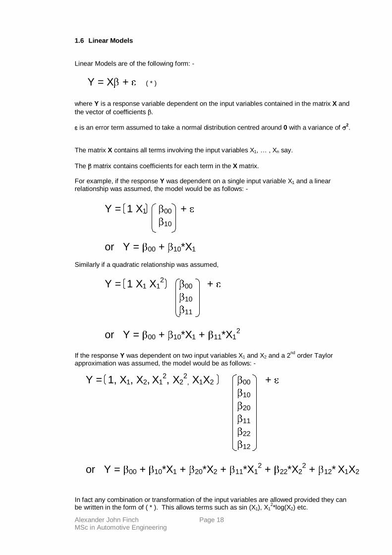
1.6 Linear Models Linear Models are of the following form: -
Y = X� + � ( * ) where Y is a response variable dependent on the input variables contained in the matrix X and the vector of coefficients ��. �� is an error term assumed to take a normal distribution centred around 0 with a variance of ��2. The matrix X contains all terms involving the input variables X1, … , Xn say. The �� matrix contains coefficients for each term in the X matrix. For example, if the response Y was dependent on a single input variable X1 and a linear relationship was assumed, the model would be as follows: -
Similarly if a quadratic relationship was assumed, If the response Y was dependent on two input variables X1 and X2 and a 2nd order Taylor approximation was assumed, the model would be as follows: - In fact any combination or transformation of the input variables are allowed provided they can be written in the form of ( * ). This allows terms such as sin (X1), X1
2*log(X2) etc.
Y = 1 X1 �00 + � �10
or Y = �00 + �10*X1
Y = 1 X1 X12 �00 + �
�10
�11
or Y = �00 + �10*X1 + �11*X1
2
Y = 1, X1, X2, X12, X2
2, X1X2 �00 + �
�10
�20
�11 �22 �12 or Y = �00 + �10*X1 + �20*X2 + �11*X1
2 + �22*X22 + �12* X1X2

Alexander John Finch Page 19 MSc in Automotive Engineering
1.61 Least squares model fitting
Given data yi, x1i, x2i, ……., xni i = 1, ….. , n. How do we decide what values the coefficients in the �� matrix should take? The traditional way is to minimise the residual sum of squares, RSS. Consider the following plot and fitted line: -
The line was fitted by minimising the square of the distance between each data point and the potential fitted line. This distance is known as the residual – see appendix II. The following plot shows the residuals in red: -
Since residuals can be both positive and negative, to stop them cancelling each other out they are squared. The residual sum of squares is then calculated: -
� ���
��
n
iii yyRSS
1
ˆ where yiˆ is the fitted value of response.
The �� matrix of coefficients minimising RSS is known as the least squares estimator and is
denoted �̂ .

Alexander John Finch Page 20 MSc in Automotive Engineering
In fact there is a neat formula to calculate �̂ , thus
� � YXXXTT 1ˆ �
�� - see reference [5].
Example, Recall the linear relationship between Y and a single input variable X1.
Suppose we sample the data points ( y1, x1 ) = ( 2, 1 ) and ( y2, x2 ) = ( 4, 4 ) Then
Hence, � � ��
���
���
���
���
���
���
���
��
�
����
�
�
����
�
�
��
4
2
41
11
41
11
41
11ˆ
1
1
TT
TT
YXXX�
��
�
�
��
�
��
32
34
The fitted line is therefore XXy 132
34ˆ �� �
The following plot shows both points and the fitted line.
Y = 1 X1 �00 �10
Y = y1 X = 1 x1 y2 1 x2

Alexander John Finch Page 21 MSc in Automotive Engineering
The line passes through both points, hence RSS = 0, the minimum value it can take. This is exactly what you would expect when fitting a line to a pair of points. The same formula holds for all linear models – see reference [5]. 1.62 Estimating the Variance The variance of a linear model can be estimated using the following formula
� � � �� �pn
XyXys
T
�
�� ˆˆ2
of an (nxp) X matrix.
i.e. n data points have been sampled modelled by p coefficients.
Note that s2 is unchanged by scaling X since �̂ will change accordingly to maintain the
value of response. 1.63 The Variance/Covariance matrix The linear models above are based on classical statistics and assume that the matrix �� is fixed.
In Bayesian Linear Models the �� matrix varies with the addition of new testpoints. Hence initially
it is given a prior distribution, �� ~ N (��0, �2 ��0 ).
��0 is the prior for the model coefficients.
��0 is the prior for the variance/covariance matrix and contains variance terms for each
coefficient down it’s leading diagonal. Since we assume the coefficients to be independent all
the covariance terms are zero.
For example, consider the 2nd order Taylor approximation where
�� = [�00 �10 �20 �11 �22 �12 ]T .
��0 is given by: -

Alexander John Finch Page 22 MSc in Automotive Engineering
������������
�
�
������������
�
�
��
��
��
���
�
��
��
���
�
���
�
��
��
���
�
���
�
���
�
��
��
���
�
���
�
���
�
���
�
��
��
���
�
���
�
���
�
���
�
���
�
��
�
���
�����
�������
���������
�����������
12
2
122222
2
1211221111
2
12202220112020
2
121022101110201010
2
1200220011002000100000
2
,cov.
,cov,cov
,cov,cov,cov
,cov,cov,cov,cov
,cov,cov,cov,cov,cov
s
s
s
s
s
s
sym
or ��0 =
������������
�
�
������������
�
�
��
��
��
��
��
��
��
��
��
��
��
��
�
�
�
�
�
�
12
2
22
2
11
2
20
2
10
2
00
2
00000
00000
00000
00000
00000
00000
s
s
s
s
s
s
where
��
0000
2variances ��
���
��
As the model coefficients are updated after each testpoint so is the variance/covariance matrix given by: - �� = �2 (��0-1 + XTX )-1 which has the same form as �0 .
1.63 Modelling engine data
Functions used for sampling testpoints throughout this report were all created using engine data
from a 2.0 litre Ford zetec engine. Units have been specified where possible.
Variances for each model were estimated using the formula from section 1.62.
Scaling of the input variables X1 X2 has also been used where appropriate – see scaling the
input variables - section 5.

Alexander John Finch Page 23 MSc in Automotive Engineering
2. Programming the Bayesian method .
2.1. MATLAB Program Details .
Details of initial Bayesian program can be found in appendix I.
The program prompts the user for the model variance, prior information for the model
coefficients and a number of testpoints.
Testpoints are then sampled randomly from a pre-determined function.
Each iteration of the main program loop takes a single data point and calculates the posterior
distribution. The posterior is then set as the new prior.
N.B. Notation - throughout the report there will be frequent references to prior information for
the model coefficients. Where all coefficients are given the same prior mean and variance then
the prior information will be denoted as follows, { 0 | 100 } indicating that all coefficients have a
mean value of 0 and a variance term of 100. Where the coefficients take different values they
will be specified separately. i.e. { 1, 2, 3 | 10, 10, 10 } indicates �00 ~N( 1, 10 ), �10 ~N( 2, 10 ),
�11 ~N( 3, 10 ).
After each testpoint is sampled a subplot of the sampling function (shown in magenta), the
current model (shown in black) and the previous model (shown in dashed red) are displayed;
indicating the ability of the model to converge.

Alexander John Finch Page 24 MSc in Automotive Engineering
2.2 Demonstration of prior knowledge on convergence .
2.21 Quadratic functions .
The sampling function was Torque = 2.2 + 11.73*throttle - 0.26*throttle^2, i.e. y = Torque (Nm),
x = throttle angle (0-10�), �00 = 2.2, �10 = 11.73 and �11 = -0.26 - see least squares model fitting.
Three different levels of prior knowledge for the model coefficients (poor, none and good) were
tested together with four different sets of variances for the model coefficients.
16 test points were sampled each time together with a nominal variance term. Results are
shown in table 2.2a
Prior Knowledge Variances
Figure.
Poor { 100, 100, 100 1 } 2.2a 10 } 2.2b 100 } 2.2c 1000 } 2.2d None { 0, 0, 0 1 } 2.2e 10 } 2.2f 100 } 2.2g 1000 } 2.2h Good { 2, 11, 0 1 } 2.2I 10 } 2.2j 100 } 2.2k 1000 } 2.2l
Table 2.2a
Figure 2.2a Figure 2.2b
Figure 2.2c Figure 2.2d

Alexander John Finch Page 25 MSc in Automotive Engineering
Figure 2c Figure 2d
Figure 2.2e Figure 2.2f
Figure 2.2g Figure 2.2h
Figure 2.2j Figure 2.2i
Figure 2.2k Figure 2.2l
Alexander John Finch Page 26 MSc in Automotive Engineering
With poor prior information and coefficient variances all equal to 1 the graphs do eventually
converge, but to a function which is different to the sampling function. With a coefficient
variance of 10 the graphs converge to the sampling function after about 10 test points have
been sampled.
With variances of 100 and 1000 the model converges after only four test points.
Poor priors with tight variances can cause the model to converge to a function other than the
one being described through the sampled data. This problem is alleviated as the coefficient
variances increase.
With no prior information and a coefficient variance of 1 convergence is achieved but is slow.
Larger coefficient variances see convergence achieved after approximately two tespoints.
With good prior information the model converges more or less after a single test point.
Good prior information clearly gives an advantage in terms of convergence time.
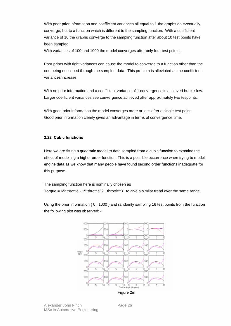
2.22 Cubic functions
Here we are fitting a quadratic model to data sampled from a cubic function to examine the
effect of modelling a higher order function. This is a possible occurrence when trying to model
engine data as we know that many people have found second order functions inadequate for
this purpose.
The sampling function here is nominally chosen as
Torque = 65*throttle - 15*throttle^2 +throttle^3 to give a similar trend over the same range.
Using the prior information { 0 | 1000 } and randomly sampling 16 test points from the function
the following plot was observed: -
Figure 2m
Alexander John Finch Page 27 MSc in Automotive Engineering
Convergence of the quadratic model is more or less achieved after 6 test points.
However it has failed to capture any of the trends of the cubic function. I.e. that over the entire
range it is increasing.
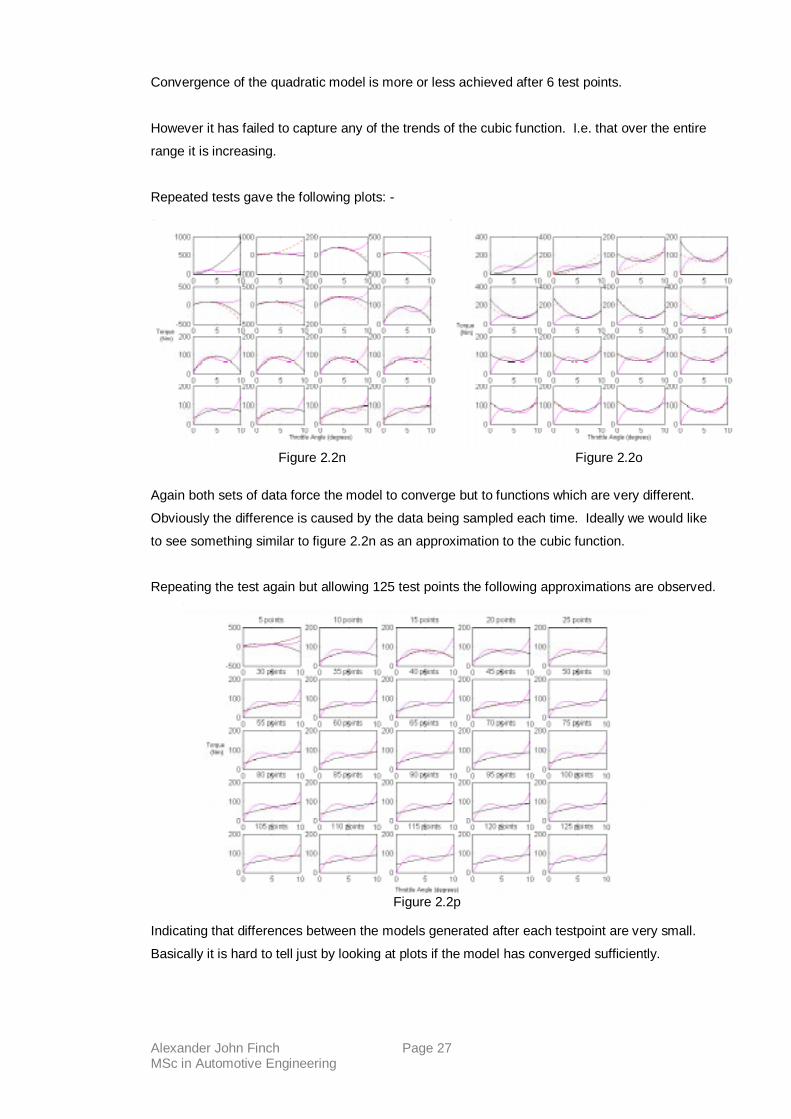
Repeated tests gave the following plots: -
Again both sets of data force the model to converge but to functions which are very different.
Obviously the difference is caused by the data being sampled each time. Ideally we would like
to see something similar to figure 2.2n as an approximation to the cubic function.
Repeating the test again but allowing 125 test points the following approximations are observed.
Indicating that differences between the models generated after each testpoint are very small.
Basically it is hard to tell just by looking at plots if the model has converged sufficiently.
Figure 2.2n Figure 2.2o
Figure 2.2p

Alexander John Finch Page 28 MSc in Automotive Engineering
If we look at plots of the model coefficients after 125 points the following is observed: -
It is clear that �00 and �10 are correlated i.e. when one increases the other decreases.
In fact you can see that they are negatively correlated from the variance/covariance matrix.
Posterior Mean =
�
�
�
�
0.0578-
5.2900
47.1666
Posterior Variance =
� �� �
�
�
�
�
0.0002 0.0015- 0.0022
0.0015- 0.0150 0.0253-
0.0022 0.0253- 0.0607
Observe that the influence of �11 is very small compared to the �00 and �10 indicating that it has
little influence in the model. For example at throttle = 10, torque is calculated as follows:-
torque = 47.17 + 5.29 * 10 - 0.058 *10^2
= 47.17 + 52.9 - 5.8
= 94.27 i.e. the throttle2 term makes up 6% of the total.
In this case we could therefore ignore the �11 term and simplify the model to a line.
So considering that the throttle^2 term has little effect it is easy to imagine how the other terms
are correlated. If the intercept �00 increases then to minimise the residual sum of squares the
gradient of the line �10 must decrease and vice versa.
The other thing to note about this plot is that the coefficients do not appear to converge. i.e.
with each new test point the model parameters change. The reason for this is simply that points
are being sampled from a cubic function so the fitted curve must constantly change. Extend the
plots to 1000 test points and the following is observed:-
Figure 2q

Alexander John Finch Page 29 MSc in Automotive Engineering
Here the plots eventually stabilise as the influence of a single test point becomes less and less.
After 1000 testpoints the coefficients are
Posterior Mean =
�
�
�
�
0.0196-
5.6602
47.3463
So we are probably safe in assuming that the ‘true’ parameters for this quadratic fit are �00 = 47,
�10 = 5.5 and �11 = 0.
Using this as prior information for the parameters and running the tests for 125 points the
following is observed:-
Figure 2r
Alexander John Finch Page 30 MSc in Automotive Engineering
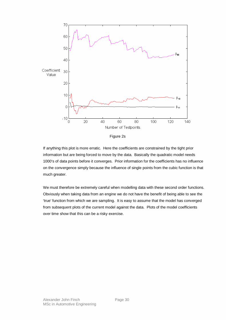
If anything this plot is more erratic. Here the coefficients are constrained by the tight prior
information but are being forced to move by the data. Basically the quadratic model needs
1000‘s of data points before it converges. Prior information for the coefficients has no influence
on the convergence simply because the influence of single points from the cubic function is that
much greater.
We must therefore be extremely careful when modelling data with these second order functions.
Obviously when taking data from an engine we do not have the benefit of being able to see the
‘true’ function from which we are sampling. It is easy to assume that the model has converged
from subsequent plots of the current model against the data. Plots of the model coefficients
over time show that this can be a risky exercise.
Figure 2s

Alexander John Finch Page 31 MSc in Automotive Engineering
2.23 Residual plots
One way to overcome the problem of modelling higher order functions is to check the fit of your
model using residual plots - see appendix II.
Here are residual plots for throttle angle and torque after 125 points.
The cubic element not captured by the model is clearly visible. In fact even if we simply see
patterns in the residuals then there is something wrong with the model assumptions.
Figure 2t Figure 2u

Alexander John Finch Page 32 MSc in Automotive Engineering
3. Model Convergence
3.1 Convergence Criteria .
We have seen previously how good prior information can increase the ability of the model to
converge and also that the model can appear to converge to a different function given a
sufficiently tight prior.
How can we quantify convergence given that the model assumptions are valid and that prior
information is representative of our knowledge of the system?
Using the model coefficients as a method of convergence seems the obvious choice but the
problem of deciding when to stop taking test points remains.
The other problem is that real data is only ever approximated by a mathematical function. Many
times the fitted model will pass through very few of the actual data points.
As testpoints are sampled subsequent estimates of the model can cover a large range of y-
values. This is because with each new testpoint the fitted model changes to accommodate the
new information
Take the following plots of the quadratic model on the same axes.
Figure 3.1a

Alexander John Finch Page 33 MSc in Automotive Engineering
The ability of the model coefficients to vary from testpoint to testpoint cause the plots to cover a
wide band of the y-axis. Any curve lying within the thick red band should provide a decent
approximation to the data. We therefore take the mean value of torque across the range of
throttle angle after each testpoint and fit a second order curve using least squares. Figure 3.1b
shows the mean values at a series of points and the least squares approximation.
Subsequent values of these new parameters should therefore be closer together and the
influence of a single point should be lessened significantly.
For example,
Figure 3.1b

Alexander John Finch Page 34 MSc in Automotive Engineering
- shows clearly the smoothing effect this process has on the coefficients.
Although the smoothed lines do flatten out completely after 100 test points the smooth nature of
the curve allows us to specify the degree of convergence required.
There is obviously some tolerance of function to be met in the variability of model parameters
since one of the aims is to minimise the number of testpoints taken to create the model. I.e. in
the above plot convergence has more or less occurred after about 60 testpoints.
It was decided that the convergence criteria would be based on the variability of subsequent
estimates of the model parameters over the previous 10 testpoints. I.e. the difference between
the maximum and minimum differences of subsequent coefficient estimates.
Consider the following theoretical plot of testpoints against coefficient values: -
Figure 3.1c
Figure 3.1d
00.10.20.30.40.50.6
0 2 4 6 8 10 12
Number of testpoints
Coe
ffici
ent V
alue

Alexander John Finch Page 35 MSc in Automotive Engineering
The minimum difference between subsequent estimates is 0.1 i.e. points 3 and 4. The
maximum difference is 0.3 between points 7 and 8. So the convergence criteria over the range
of 10 testpoints is 0.3 – 0.1 = 0.2.
In theory this should work effectively but it does depend on knowing the range of values the
coefficients are likely to take in order to specify a sensible difference. Since prior knowledge of
these ranges is not always available the criteria will have to be based on the ranges provided by
the model approximations during testing. i.e. as a percentage of the current model coefficients.
Although this does mean that the convergence criteria will be continually changing it is the only
way to provide the correct scale. On the other hand you will have to specify some percentage
of the model coefficients which is also a bit of a guessing game. But it is more intuitive to allow
a 1% error in the coefficients than it is to allow a fixed difference. What difference this
percentage actually makes will have to be determined from testing.

Alexander John Finch Page 36 MSc in Automotive Engineering
3.2 Effect of prior knowledge on convergence times
3.21 Convergence of Quadratic functions
Convregence criteria is tested here using the function Torque = 2.2 + 11.73*throttle -
0.26*throttle^2.
Different levels of convergence criteria and prior information were tested using random
sampling from the function above. The results are shown below in table 3.2a
Convergence criteria Prior Convergence times
( Number of testpoints )
1.5% { 0 | 1 } 21,21,21
{ 0 | 10 } 21,21,21
{ 0 | 100 } 21,21,21
{ 0 | 1000 } 22,22,22
1.0% { 0 | 1 } 23,24,23
{ 0 | 10 } 23,23,24
{ 0 | 100 } 23,23,23
{ 0 | 1000 } 23,23,23
0.5% { 0 | 1 ] 38,27,28,40
{ 0 | 10 } 27,27,35,46
{ 0 | 100 } 27,27,27,26
{ 0 | 1000 } 27,42,26,27
All these models converged to the model values.
It's fairly easy to see that as the convergence criteria gets tighter the models take longer to
converge.
Differences in convergence times for increasing variances are negligible for convergence
criteria of 1.5% and1.0%. When the criteria is set to 0.5% we observe a large variability in the
convergence time. There will be some differences observed because of the random sampling
taking place but large variations must be occurring by another means.
Table 3.2a

Alexander John Finch Page 37 MSc in Automotive Engineering
Observe the following time series plots of the data points for convergence criteria of 0.5%, prior
{ 0 | 1 } when convergence is achieved after 40 and 28 testpoints respectively:-
The basic difference between these plots seems to be that quicker convergence is achieved
when the testpoints are nicely spaced. Figure 3.2a is characterised by large steps across the
range followed by a series of testpoints bunched together. As the testpoints 'jump' across the
range the model parameters are changed significantly hindering convergence.
It is also the case that data from across the range is collected within approximately five points
so that significant changes in the model coefficients are avoided.
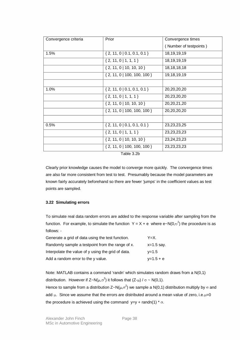
Table 3.2b shows the same tests with a good prior knowledge.
Figure 3.2a Figure 3.2b
Alexander John Finch Page 38 MSc in Automotive Engineering
Convergence criteria Prior Convergence times
( Number of testpoints )
1.5% { 2, 11, 0 | 0.1, 0.1, 0.1 } 18,19,19,19
{ 2, 11, 0 | 1, 1, 1 } 18,19,19,19
{ 2, 11, 0 | 10, 10, 10 } 18,18,18,18
{ 2, 11, 0 | 100, 100, 100 } 19,18,19,19
1.0% { 2, 11, 0 | 0.1, 0.1, 0.1 } 20,20,20,20
{ 2, 11, 0 | 1, 1, 1 } 20,23,20,20
{ 2, 11, 0 | 10, 10, 10 } 20,20,21,20
{ 2, 11, 0 | 100, 100, 100 } 20,20,20,20
0.5% { 2, 11, 0 | 0.1, 0.1, 0.1 } 23,23,23,25
{ 2, 11, 0 | 1, 1, 1 } 23,23,23,23
{ 2, 11, 0 | 10, 10, 10 } 23,24,23,23
{ 2, 11, 0 | 100, 100, 100 } 23,23,23,23
Table 3.2b
Clearly prior knowledge causes the model to converge more quickly. The convergence times
are also far more consistent from test to test. Presumably because the model parameters are
known fairly accurately beforehand so there are fewer ‘jumps’ in the coefficient values as test
points are sampled.
3.22 Simulating errors
To simulate real data random errors are added to the response variable after sampling from the
function. For example, to simulate the function Y = X + e where e~N(0,�2) the procedure is as
follows: -
Generate a grid of data using the test function. Y=X.
Randomly sample a testpoint from the range of x. x=1.5 say.
Interpolate the value of y using the grid of data. y=1.5
Add a random error to the y value. y=1.5 + e
Note: MATLAB contains a command ‘randn’ which simulates random draws from a N(0,1)
distribution. However if Z~N(�,�2) it follows that (Z-�) / � ~ N(0,1).
Hence to sample from a distribution Z~N(�,�2) we sample a N(0,1) distribution multiply by � and
add �. Since we assume that the errors are distributed around a mean value of zero, i.e.�=0
the procedure is achieved using the command y=y + randn(1) * �.

Alexander John Finch Page 39 MSc in Automotive Engineering
3.23 Convergence to quadratic functions with simulated errors.
The same quadratic function is used but with the addition of simulated errors.
Using a model variance �2 = 140 and a series of prior information the convergence criteria were
tested.
Table 3.2c displays the results.
Convergence criteria Prior Convergence times
1.5% { 0 | 1 } 62,40,64,54,50,47,31,45,55,44
{ 0 | 10 } 41,52,32,68,59,51,61,39,54,56
{ 0 | 100 } 44,56,40,53,67,47,44,75,68,60
{ 0 | 1000 } 69,51,60,44,53,40,57,67,56,146
1.0% { 0 | 1 } 105,57,72,75,36,85,55,68,67,54
{ 0 | 10 } 100,45,66,58,42,62,40,37,76,45
{ 0 | 100 } 79,69,53,148,62,52,57,77,76,74
{ 0 | 1000 } 47,47,68,62,46,47,39,50,61,64
0.5% { 0 | 1 } 62,112,77,86,130,80,67,61,93,70
{ 0 | 10 } 157,54,60,160,125,79,96,72,71,124
{ 0 | 100 } 75,122,103,88,82,101,70,69,87,125
{ 0 | 1000 } 70,81,57,72,100,69,98,108,56,72
Table 3.2c
There is a lot of variability in a single sample of convergence times. Therefore to compare two
samples we look for differences in the distribution of the mean values– see appendix III.
From statistical tests there is a statistically significant difference between the mean values when
comparing convergence criteria of 1.5% to 1.0% and also comparing 1.0% to 0.5%.
Tests show that there is not a significant difference for a fixed convergence level and different
prior variances.
We expect to see some variation in the convergence times for a single sample due to the
random sampling and the addition of random errors. As previously, the most significant
difference between high and low convergence times from the same sample is the way in which
testpoints are selected.
Figure’s 3.2c and 3.2d show time series plots of testpoints for a prior of { 0 | 1 } and
convergence times of 40 and 64 respectively.

Alexander John Finch Page 40 MSc in Automotive Engineering
Figure 3.2d shows the characteristic bunching and large steps between neighbouring data
points seen previously. We also see that the full range of data is not exploited until well into the
sampling. Combinations of these factors cause the model parameters to ‘jump’ hindering the
convergence criteria.
In fact these patterns are to be observed in nearly all the models with larger convergence times.
Table 3.2d shows the same tests with good prior knowledge of the model coefficients.
Convergence criteria Prior Convergence times
( Number of testpoints )
1.5% { 2, 11, 0 | 0.1, 0.1, 0.1 } 31,39,41,52,64,47,28,52,32,53
{ 2, 11, 0 | 1, 1, 1 } 36,59,37,48,42,59,45,32,37,68
{ 2, 11, 0 | 10, 10, 10 } 37,32,40,78,53,46,70,36,76,80
{ 2, 11, 0 | 100, 100, 100 } 41,65,53,74,46,62,74,36,51,60
1.0% { 2, 11, 0 | 0.1, 0.1, 0.1 } 30,39,41,24,73,43,61,49,68,49
{ 2, 11, 0 | 1, 1, 1 } 62,48,89,46,70,68,47,47,50,45
{ 2, 11, 0 | 10, 10, 10 } 51,49,66,46,34,78,58,81,42,91
{ 2, 11, 0 | 100, 100, 100 } 58,67,64,69,80,61,54,83,36,73
0.5% { 2, 11, 0 | 0.1, 0.1, 0.1 } 56,44,63,59,56,39,107,61,81,64
{ 2, 11, 0 | 1, 1, 1 } 55,100,67,95,70,93,92,123,61,62
{ 2, 11, 0 | 10, 10, 10 } 52,71,151,100,84,90,76,73,81,105
{ 2, 11, 0 | 100, 100, 100 } 76,104,120,85,57,71,57,128,77,60,
Table 3.2d
Figure 3.2c Figure 3.2d

Alexander John Finch Page 41 MSc in Automotive Engineering
Tests show that the prior variance for the model coefficients makes no difference to the
convergence times for a given criteria.
There are significant differences in convergence between all three convergence criteria.
The convergence criteria appear to work well for quadratic functions.
When comparing good prior knowledge to no prior knowledge there appears to be no significant
difference in convergence times. One possible explanation for this might be the fact that the
variance is so great, causing large differences in the fitted models. I.e. they converge to
something other than the sampling function. The variance was so great because the original
model was such a poor fit to the data
Table 3.2e shows a comparison of good prior knowledge to no prior knowledge for a
convergence criteria of 0.5% and a reduced variance of �2 = 10.
Convergence criteria Prior Convergence times
( Number of testpoints )
0.5% { 2, 11, 0 | 0.1, 0.1, 0.1 } 50,38,27,29,34,36,3842,37,37
32,36,38,32,42,37,34,34,34,22
40,43,38,43,30,42,30,36,29,41
42,26,25,34,28,26,36,40,45,42
0.5% { 0 | 100 } 62,42,55,53,53,50,37,55,58,60
72,56,42,48,42,38,56,53,61,40
66,48,34,54,46,57,47,36,44,55
69,52,50,53,65,92,54,63,51,38
Table 3.2e
Here there is a statistically significant difference between the means. The mean of the first
sample is 35.63 compared to the mean of the second sample 52.68. This is a significant saving
in testing time. We therefore require the model to be a good fit to the data for prior knowledge
to make a significant difference.

Alexander John Finch Page 42 MSc in Automotive Engineering
3.24 Convergence to cubic equations .
Using the sampling function Torque = Throttle^3 –15*Throttle^2 +65*Throttle across a range of
0-10� the process for testing convergence criteria was repeated.
Results are shown in table 3.2f.
Convergence criteria Prior Convergence times
( Number of testpoints )
1.5% { 0 | 1 } 35,37,23,30,47,39,58,41,74,48
{ 0 | 10 } 26,77,30,63,70,74,66,31,58,33
{ 0 | 100 } 39,64,35,26,60,42,33,39,110,26
{ 0 | 1000 } 65,35,53,65,48,36,44,57,70,33
1.0% { 0 | 1 } 95,86,35,32,29,57,48,54,78,44
{ 0 | 10 } 54,109,103,90,46,49,32,86,53,34
{ 0 | 100 } 70,62,74,54,63,56,36,89,32,37
{ 0 | 1000 } 27,36,92,43,73,57,61,74,67,83
0.5% { 0 | 1 } 39,39,49,89,41,60,51,65,46,41
{ 0 | 10 } 63,81,58,84,83,69,63,41,136,49
{ 0 | 100 } 43,83,59,90,88,65,50,79,74,56
{ 0 | 1000 } 71,124,66,69,56,87,28,88,31,75
Table 3.2f
Statistical comparisons showed there to be no significant difference between priors for a given
convergence criteria.
N.B. Since we find no difference between prior variances for the same convergence criteria all
samples can be grouped for more accurate comparison to the others.
A significant difference in convergence time is detected between 1.5% and 1.0% and also
between 1.5% and 0.5%. No difference was detected between 1.0% and 0.5%.
The convergence criteria appear to be working except that there is a very large variation in the
convergence times.
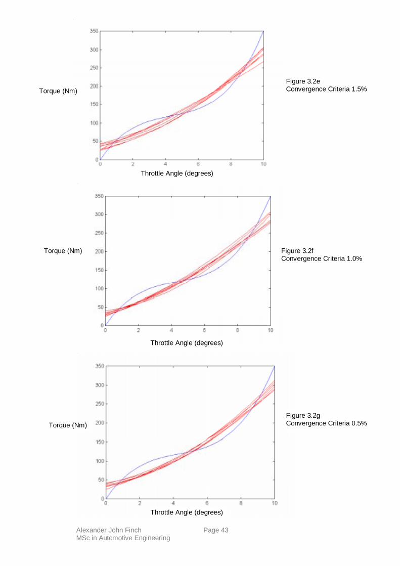
It is very easy for quadratic functions to converge to many different models when the sampling
is random and from a cubic function. This is easily seen if we plot the sampling function and a
selection of quadratic models for a given convergence criteria – see figures 3.2e, 3.2f and 3.2g.
Alexander John Finch Page 43 MSc in Automotive Engineering
Torque (Nm)
Torque (Nm)
Torque (Nm)
Throttle Angle (degrees)
Throttle Angle (degrees)
Throttle Angle (degrees)
Figure 3.2e Convergence Criteria 1.5%
Figure 3.2f Convergence Criteria 1.0%
Figure 3.2g Convergence Criteria 0.5%
Alexander John Finch Page 44 MSc in Automotive Engineering
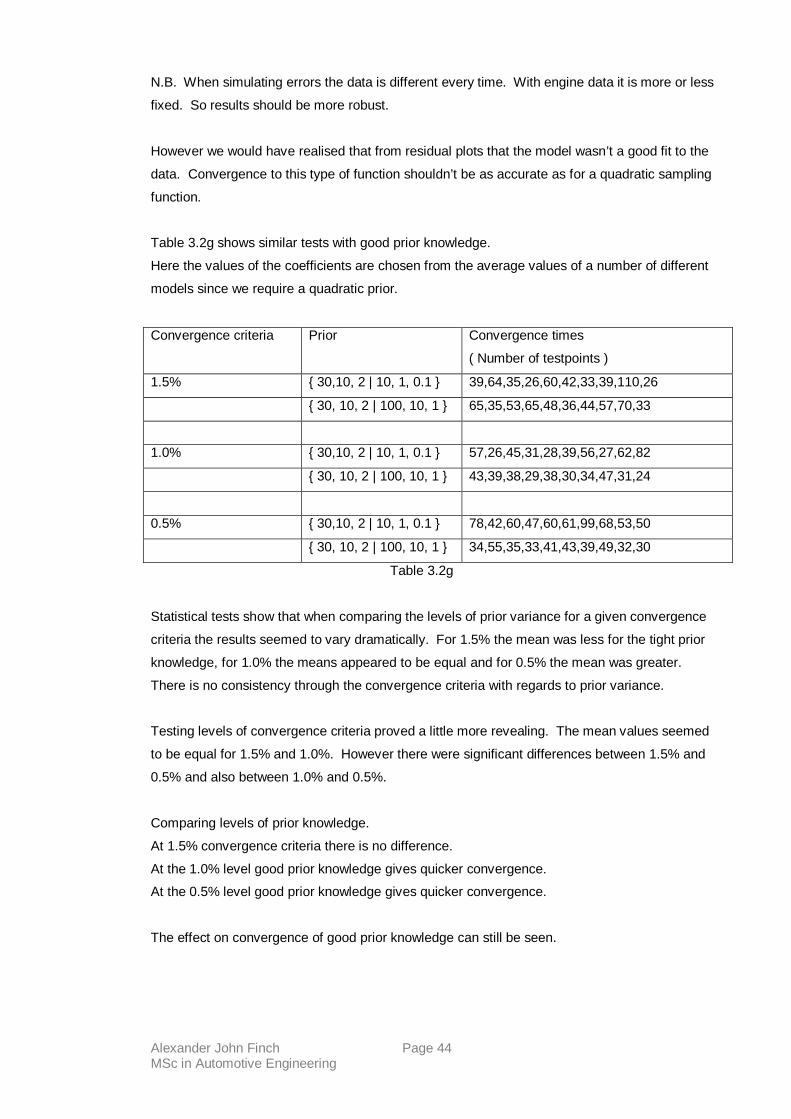
N.B. When simulating errors the data is different every time. With engine data it is more or less
fixed. So results should be more robust.
However we would have realised that from residual plots that the model wasn’t a good fit to the
data. Convergence to this type of function shouldn’t be as accurate as for a quadratic sampling
function.
Table 3.2g shows similar tests with good prior knowledge.
Here the values of the coefficients are chosen from the average values of a number of different
models since we require a quadratic prior.
Convergence criteria Prior Convergence times
( Number of testpoints )
1.5% { 30,10, 2 | 10, 1, 0.1 } 39,64,35,26,60,42,33,39,110,26
{ 30, 10, 2 | 100, 10, 1 } 65,35,53,65,48,36,44,57,70,33
1.0% { 30,10, 2 | 10, 1, 0.1 } 57,26,45,31,28,39,56,27,62,82
{ 30, 10, 2 | 100, 10, 1 } 43,39,38,29,38,30,34,47,31,24
0.5% { 30,10, 2 | 10, 1, 0.1 } 78,42,60,47,60,61,99,68,53,50
{ 30, 10, 2 | 100, 10, 1 } 34,55,35,33,41,43,39,49,32,30
Table 3.2g
Statistical tests show that when comparing the levels of prior variance for a given convergence
criteria the results seemed to vary dramatically. For 1.5% the mean was less for the tight prior
knowledge, for 1.0% the means appeared to be equal and for 0.5% the mean was greater.
There is no consistency through the convergence criteria with regards to prior variance.
Testing levels of convergence criteria proved a little more revealing. The mean values seemed
to be equal for 1.5% and 1.0%. However there were significant differences between 1.5% and
0.5% and also between 1.0% and 0.5%.
Comparing levels of prior knowledge.
At 1.5% convergence criteria there is no difference.
At the 1.0% level good prior knowledge gives quicker convergence.
At the 0.5% level good prior knowledge gives quicker convergence.
The effect on convergence of good prior knowledge can still be seen.

Alexander John Finch Page 45 MSc in Automotive Engineering
3.25 Convergence to cubic equations with simulated errors.
The same cubic function is used but with the addition of simulated errors.
Using a model variance, �2 = 140 and a series of prior information the convergence criteria were
tested. Table 3.2h displays the results.
Convergence criteria Prior Convergence times
( Number of testpoints )
1.5% { 0 | 1 } 26,23,36,36,32,28,31,44,31,30
{ 0 | 10 } 52,28,38,33,32,53,34,47,31,35
{ 0 | 100 } 38,30,28,25,38,30,36,21,64,33
{ 0 | 1000 } 33,44,38,36,40,32,38,41,30,40
1.0% { 0 | 1 } 54,39,45,36,33,32,40,52,38,34
{ 0 | 10 } 45,36,58,52,44,45,106,49,46,40
{ 0 | 100 } 44,35,51,45,40,67,55,54,35,42
{ 0 | 1000 } 32,39,41,36,43,41,32,67,56,72
0.5% { 0 | 1 } 50,61,39,38,53,51,46,43,43,46
{ 0 | 10 } 57,37,46,61,65,54,45,55,62,57
{ 0 | 100 } 137,88,45,37,55,51,63,84,52,58
{ 0 | 1000 } 56,45,57,81,49,39,44,68,47,95
Table 3.2h
Tests show that there are no differences in the mean values between the level of prior
variances for a given convergence criteria.
There are significant differences in convergence from 1.5% to 1.0% and from 1.0% to 0.5%.
Table 3.2i shows similar tests with good prior knowledge.
Convergence criteria Prior Convergence times
( Number of testpoints )
1.5% { 30, 10, 2 | 10, 1, 0.1 } 71,42,28,29,35,74,25,34,41,35
{ 30, 10, 2 | 100, 10, 1 } 34,45,27,46,34,35,33,48,43,32
1.0% { 30, 10, 2 | 10, 1, 0.1 } 43,35,37,105,48,87,37,41,38,42
{ 30, 10, 2 | 100, 10, 1 } 58,41,49,52,58,38,36,58,35,62
0.5% { 30, 10, 2 | 10, 1, 0.1 } 38,51,63,48,41,52,52,54,41,54
{ 30, 10, 2 | 100, 10, 1 } 42,68,58,51,44,98,69,51,46,39
Table 3.2i

Alexander John Finch Page 46 MSc in Automotive Engineering
N.B. In these sorts of sample sizes one large observation can distort the variance quite
dramatically.
Tests show there to be no difference between prior variances for all convergence criteria.
There are significant differences in convergence between 1.5% and 1.0% and also between
1.5% and 0.5%. i.e. it took longer to converge on average for tighter convergence criteria.
Comparing levels of prior knowledge.
At the 1.5% level there is no difference.
At the 1.0% level there is no difference.
At the 0.5% level there is no difference.
There is no significant difference between no prior knowledge and good prior knowledge.
The same thing was observed when modelling the quadratic with simulated errors combined
with a large model variance.
The fact that we are trying to model a higher order function coupled with a large variance
causes large differences in convergence of the fitted models.
Table 3.2j shows a comparison of good prior knowledge to no prior knowledge for a
convergence criteria of 0.5% and a reduced variance of 10.
Convergence criteria Prior Convergence times
0.5% { 30, 10, 2 | 100, 10, 1 } 55, 90, 72, 57, 59, 117, 72, 87, 78, 41
52, 73, 62, 74, 100, 54, 140, 75, 138, 42
72, 74, 63, 104, 143, 42, 82, 60, 52, 64
133, 34, 126, 78, 58, 75, 77, 93, 93, 36
0.5% { 0 | 100 } 146, 86, 84, 124, 74, 63, 86, 87, 104, 59
48, 71, 61, 109, 51, 99, 33, 80, 120, 66
131, 148, 51, 31, 73, 52, 57, 65, 88, 53
117, 84, 93, 72, 73, 146, 28, 138, 71, 71
Table 3.2e
Statistical tests show there to be no difference in convergence between no prior knowledge and
good prior knowledge. In section 3.22 the lower variance represented data that could be
modelled well by a second order function. Here the fact that errors are added to a higher order
function cause massive variations in convergence times and model coefficients for the second
order model.

Alexander John Finch Page 47 MSc in Automotive Engineering
We must therefore be careful to select a model for the data which can capture data trends in a
consistent manner. Although any failures of the current model to capture trends of the data will
be observed in the residual plots – see appendix II.
3.26 Convergence using engine data and second order Taylor approximation .
Using engine data for engine speed and torque against fuel consumption the convergence
criteria were tested again. The data contained a total of 334 points. These points were
randomly sampled.
The variance was assumed to be 0.827 from fitting a least squares model to the same data.
The fitted model was:-
Wfuel = 2.05 – 111.26*eng – 19.5 torque + 2901.19*eng2 + 55.89*torque2 + 2711.46*eng*torque
Both engine speed and torque were scaled to give the model parameters reasonable values –
see section 5. Hence prior information contains greater variances.
Table 3.2j shows results,
Convergence criteria Prior Convergence times
1.5% { 0 | 1e3 } 33,27,28,33,29,26,29,27,35,27
{ 0 | 1e4 } 42,45,31,39,45,53,47,43,35,45
{ 0 | 1e5 } 89,47,140,115,33,53,33,40,65,88
{ 0 | 1e6 } 82,52,87,55,51,40,78,37,67,64
1.0% { 0 | 1e3 } 46,32,47,59,41,34,37,39,48,41
{ 0 | 1e4 } 43,46,49,93,69,51,46,60,79,114
{ 0 | 1e5 } 40,59,113,96,87,89,52,115,88,102
{ 0 | 1e6 } 62,56,71,65,55,66,51,50,75,75
0.5% { 0 | 1e3 } 96,51,45,49,42,55,56,61,49,47
{ 0 | 1e4 } 74,66,94,55,75,72,86,79,67,55
{ 0 | 1e5 } 131,58,143,147,141,52,108,50,100,117
{ 0 | 1e6 } 70,67,73,98,86,81,56,70,70,81
Table 3.2j
When the prior is quite bad – i.e. low variance, and the convergence criteria high,1.5% - then
the model seems to converge very quickly and consistently. In this case the model converges
to values very different than expected from the least squares fitted model. The prior is so tight
that the data has little influence and convergence is forced prematurely.

Alexander John Finch Page 48 MSc in Automotive Engineering
A similar pattern can be seen for 1.5% convergence and a { 0 | 1e4 } prior. And indeed for 1.0%
convergence and { 0 | 1e3 } and { 0 | 1e4 } priors.
When the convergence criteria is at 0.5% then the same phenomenon occur only it takes longer
due to the stricter convergence criteria.
Tests show that priors of { 0 | 1e3 } are consistently quicker to converge prematurely than priors
of { 0 | 1e4 }.
Priors of { 0 | 1e5 } take consistently longer to converge than priors of { 0 | 1e6 }.
In this case the prior slows convergence but not enough to make it converge prematurely.
Overall there are significant differences in convergence between all the levels of convergence
criteria.
Table 3.2k shows results for good prior information.
Convergence criteria Prior Convergence times
1.5% { 2, -111, -19.5, 2900, 56, 2700
| 10, 1e3, 1e3, 1e3, 1e3, 1e3 }
19,19,33,19,21,28,19,20,19,20,19
17,19,17,18,23,19,28,21,21,30,23
20,22,25,24,19,23,22,22,17,18,25
26,23,17,25,21,30,23,18,30,24,17
1.0% { 2, -111, -19.5, 2900, 56, 2700
| 10, 1e3, 1e3, 1e3, 1e3, 1e3 }
29,36,19,26,27,34,22,24,23,29
30,33,24,34,26,25,26,25,24,23
22,30,27,26,32,20,19,21,21,18
19,20,18,26,22,19,18,17,21,23
0.5% { 2, -111, -19.5, 2900, 56, 2700
| 10, 1e3, 1e3, 1e3, 1e3, 1e3 }
28,28,28,40,32,31,34,36,40,35
28,37,27,29,25,43,25,26,29,23
34,33,35,29,39,26,31,26,33,38
36,33,27,45,33,41,27,32,28,30
Table 3.2k
Again there are significant differences between all levels of convergence criteria.
Significant savings in convergence are also made. For instance comparing just the { 0 | 1e6 }
priors with data from the good priors at each level of convergence we observe the following: -

Alexander John Finch Page 49 MSc in Automotive Engineering
No Prior knowledge Good Prior knowledge
Convergence criteria
Sample
mean
Sample
Variance
Sample
mean
Sample
Variance
1.5% 61.30 298.23 23.09 21.29
1.0% 62.60 87.82 26.90 28.10
0.5% 75.20 136.18 33.20 35.96
Table 3.2l
With good prior knowledge there is at least a 50% saving in convergence time. From the size of
sample variances the convergence is also far more consistent when a good prior is employed
3.27 Conclusions
If care is taken with the choice of prior then the convergence criteria are generally consistent. A
lower convergence criteria provides greater convergence times and vice versa.
Convergence times are not affected by the prior variance for the model coefficients.
Poor tight prior knowledge causes the model to converge quickly but to a poor approximation of
the data sampled.
Provided the data can be accurately modelled by a second order function then good prior
knowledge of the model coefficients offers significant savings in convergence time.
If however we try to model higher order functions convergence is not affected by the level of
prior knowledge. When data is randomly sampled from a cubic function then quadratic
approximations will be extremely variable. Therefore prior knowledge for these quadratics will
also be extremely varied. Second order prior knowledge of a third order system is poor by
definition.
The failure of a model to capture trends in the data will be revealed in the residual plots. In this
way time need not be wasted pursuing the current model. In fact the data can still be used to
model a higher order function as soon as trends in the residual plots are observed – see
appendix II.
Since the idea is to minimise the number of testpoints sampled, modelling higher order systems
with lower order functions should not be attempted.
Significant differences in convergence times were observed using criteria of 1.5%, 1.0% and
0.5%. Repeated trials using different criteria would need to be carried out to assess the effect
the convergence criteria had on the quality of the fitted model. I.e. there is probably an optimum

Alexander John Finch Page 50 MSc in Automotive Engineering
criteria given a particular dataset to simultaneously optimise the number of testpoints taken and
to provide a good fitting model.
Convergence is also greatly affected by the way in which data is collected.
When data from across the range of the input variable is gathered quickly then convergence is
quicker. This leaves less scope for the coefficients to vary.
In the case of the engine data, although sampling is random from the set of points, the data is
not. A plot of the data shows that most of it is concentrated in one area – presumably where the
most useful information lies. In this way, if all data points come from this area the model
converges quickly. If a few points are sampled away from this area then the model changes
significantly, hindering the convergence.
Ideally data would be taken at random from across the range. If however one area is of more
interest then the model should stick to that range. This will capture more information and help
convergence to be more consistent.
Note that if during sampling a coefficient of the model is converging to zero then the
convergence criteria can breakdown. I.e. as the coefficient gets smaller so does the margin of
error , given by a percentage of the coefficient. Hence convergence may never be achieved. A
clause in the program which looks at the percentage of response each coefficient contributes
could be used to alleviate this problem. I.e. if we identify a coefficient converging zero -
measure the percentage of response it contributes to the model. If the response is less than
1% say then ignore it for convergence purposes.

Alexander John Finch Page 51 MSc in Automotive Engineering
4. Model Assessment
4.1 Confidence Intervals. (C.I.’s)
4.11 What are Confidence Intervals?
Confidence intervals express our belief about the possible variability of the current model given
the data sampled so far.
For example a 95% C.I. is the range for the model for which we are 95% certain the true model
lies.
Generally the smaller the interval the more accurate the model, provided the model
assumptions remain valid.
4.12 How to calculate C.I.’s.
C.I.'s are calculated using the variability of the model coefficients found in the variance /
covariance matrix.
A (1-�)*100% C.I. is calculated using the formula -
� �ystyhpnh
ˆˆ *),
21( ��
� � - see reference [6]
Where,
� � � �xbsxys hThh
22 ˆ �
� �yy hh�ˆ
xh = range of current model. i.e. a series of points to
construct an interval.
yh= expected response from current model. I.e. the
curve
generated by the points xh.
s2(b) = variance / covariance matrix.
t(1-�), n-p = upper 1-� percentage point of the t
distribution.

Alexander John Finch Page 52 MSc in Automotive Engineering
4.13 Effect of prior knowledge on C.I.’s using functions as dat asets. One variable.
For a constant engine speed fuel consumption varies with torque as follows: -
Wfuel = 0.6081 + 1.5425*Torque + 0.2751*Torque2. Model Variance �2 = 1e-3.
Using prior knowledge { 0 | 100 } figure 4.1a shows how the C.I. decreases as the amount of
data collected increases. This is due to the increased information gained from sampling more
testpoints. I.e. the variability of the model coefficients decreases with testing.
Figure 4.1a
----- Confidence Interval --x--Current Model and testpoints
----- Confidence Interval --x--Current Model and testpoints
----- Confidence Interval --x--Current Model and testpoints
----- Confidence Interval --x--Current Model and testpoints
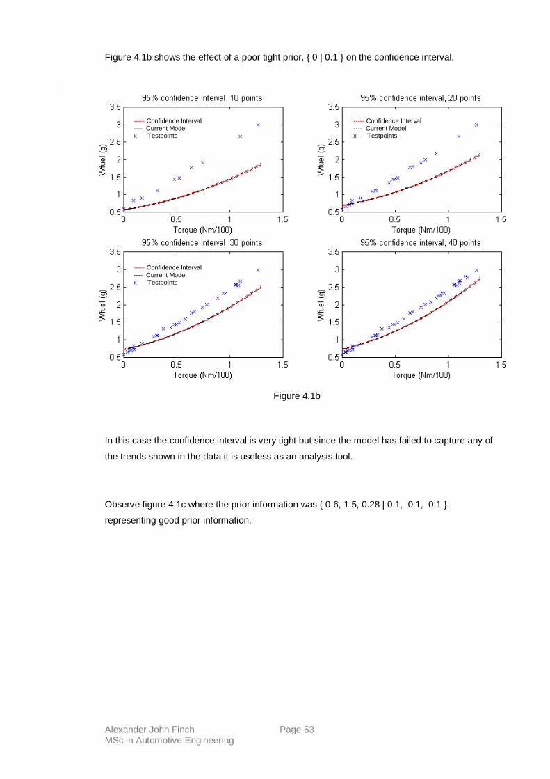
Alexander John Finch Page 53 MSc in Automotive Engineering
Figure 4.1b shows the effect of a poor tight prior, { 0 | 0.1 } on the confidence interval.
In this case the confidence interval is very tight but since the model has failed to capture any of
the trends shown in the data it is useless as an analysis tool.
Observe figure 4.1c where the prior information was { 0.6, 1.5, 0.28 | 0.1, 0.1, 0.1 },
representing good prior information.
Figure 4.1b
----- Confidence Interval ---- Current Model x Testpoints
----- Confidence Interval ---- Current Model x Testpoints
----- Confidence Interval ---- Current Model x Testpoints

Alexander John Finch Page 54 MSc in Automotive Engineering
Here confidence in the model is very high due to the quality of the prior information.
4.14 Effect of model variance on C.I.’s. One variable.
Here we attempt to answer the question: - What effect does assuming the wrong model
variance have on confidence intervals?
Using the same function as before, a prior of { 0 | 100 } and sampling data using a model
variance of �2 = 1e-3, confidence intervals were constructed for various different assumed
model variances.
Figure 4.1c
----- Confidence Interval ---- Current Model x Testpoints
----- Confidence Interval ---- Current Model x Testpoints
----- Confidence Interval ---- Current Model x Testpoints
----- Confidence Interval ---- Current Model x Testpoints

Alexander John Finch Page 55 MSc in Automotive Engineering
Figure 4.1d shows confidence intervals for an assumed model variance of �2 = 1e-2.
Here the confidence intervals are unnecessarily large.
Similarly, the more we overestimate the variance the larger the confidence intervals become.
This forces us to have less confidence in an otherwise good fitting model. One way to
overcome this is to allow �2 to vary as well as the model coefficients.
Figure 4.1d
----- Confidence Interval ---- Current Model x Testpoints
----- Confidence Interval ---- Current Model x Testpoints
----- Confidence Interval ---- Current Model x Testpoints
----- Confidence Interval ---- Current Model x Testpoints

Alexander John Finch Page 56 MSc in Automotive Engineering
Figure 4.1e shows the effect of an underestimated model variance of �2 = 1e-5.
Here there is too much confidence in the model. This might cause us to stop testing
prematurely. The solution to this problem is the same as before – give the model variance a
probability distribution.
The model variance has a dramatic effect on the width of these intervals and needs to be
evaluated exactly in order that confidence intervals might be accurate.
Figure 4.1e
----- Confidence Interval ---- Current Model x Testpoints
----- Confidence Interval ---- Current Model x Testpoints
----- Confidence Interval ---- Current Model x Testpoints
----- Confidence Interval ---- Current Model x Testpoints

Alexander John Finch Page 57 MSc in Automotive Engineering
4.15 Effect of prior knowledge on C.I.’s using functions as dat asets. Two variables.
Using the function
Wfuel = 2.05 – 11.13*Eng – 19.5 Torque + 29.01*Eng2 + 55.89*Torque2 + 271.15*Eng*Torque
, prior knowledge { 0, 0, 0, 0, 0, 0 | 10, 1e2, 1e2, 1e3, 1e3, 1e3 } and Model variance �2 = 0.827
40 testpoints were randomly sampled.
Figure 4.1f shows the observed confidence intervals: -
Again, observe how the confidence intervals get narrower as the number of testpoints
increases.
Figure 4.1f
Confidence Interval
Current model Testpoints

Alexander John Finch Page 58 MSc in Automotive Engineering
Figure 4.1i shows confidence intervals for good prior { 0, -10, -20, 30, 50, 250 | 10, 10, 10, 10,
10, 100 }.
Clearly the better the prior information the narrower the confidence intervals and hence the
more confidence we have in the model.
Figure 4.1i
Confidence Interval
Current Model
Testpoints

Alexander John Finch Page 59 MSc in Automotive Engineering
4.16 Effect of model variance on C.I.’s. Two variables.
Using a prior of { 0, 0, 0, 0, 0, 0 | 10, 1e2, 1e2, 1e3, 1e3, 1e3 } and sampling data using a
model variance of 0.827, confidence intervals were constructed for various different assumed
model variances.
Figures 4.1j, 4.1k and 4.1l show confidence intervals for assumed model variances of 0.0827,
8.27 and 82.7 respectively. 40 testpoints have been sampled.
Figure 4.1j
Confidence Interval
Current Model
Testpoints

Alexander John Finch Page 60 MSc in Automotive Engineering
As previously, the intervals widen if the assumed model variance is greater than the actual
value and shorten when the assumed variance is less.
Figure 4.1k
Confidence Interval
Current Model
Testpoints
Figure 4.1l
Confidence Interval
Current Model
Testpoints

Alexander John Finch Page 61 MSc in Automotive Engineering
Then either we are overconfident and decide to stop testing or are under confident and continue
testing unnecessarily. Allowing the model variance �2 to vary can alleviate this problem.
4.17 C.I.’s using engine-testing data.
Using the function: -
Torque = -41.04 + 103.64*Eng + 120.02*Inlet - 221.11*Eng2 + 42.53*Inlet2 + 103.67*Eng*Inlet,
prior knowledge { –40, 100, 120, -220, 40, 100 | 10, 10, 10, 10, 10, 10 } and �2 = 49.47
confidence intervals were compared from random sampling of real data and function data.
Figure’s 4.1m and 4.1n show the confidence intervals for the real data and function respectively.
Figure 4.1m

Alexander John Finch Page 62 MSc in Automotive Engineering
These confidence intervals are very similar bearing in mind they were created using different
datasets.
This gives an indication that inferences made from analysis of the functions should be valid
when using test data.
They are wide since the model variance is fairly large.
i.e. the least squares model fitted originally wasn’t a particularly good fit to the data.
Figure 4.1n
Confidence Interval
Current Model
Testpoints

Alexander John Finch Page 63 MSc in Automotive Engineering
4.18 Conclusions
Good prior information creates narrower confidence intervals and hence we can be more
confident with the current model.
However, poor priors can also create tight confidence intervals. In general this will not pose a
problem since residual plots will indicate the inability of the current model to capture the trend of
the sampled data.
Assuming a model variance greater than the actual variance of the data forces us to have less
confidence in our models. Assuming a model variance less than the actual variance and we
become overconfident in the model. The solution to this problem is to allow the model variance
to take a distribution so that it may vary as data is sampled.
Note that confidence intervals can be used as a form of convergence criteria. For example if we
want to model fuel consumption until we are accurate to within � 0.1 g then the largest part of
the interval can be measured until this is achieved.
This method is dependent on the variance of the data since this will inevitably determine the
smallest size of the confidence interval. A large model variance and we may never achieve the
desired accuracy.
Problems with poor prior information would also need to be overcome if this method of
convergence were to be employed.

Alexander John Finch Page 64 MSc in Automotive Engineering
4.2 Predictive intervals.
4.21 What are predictive intervals?
Predictive intervals express the confidence with which we can place a future observation given
the current model. They will always be wider than the confidence intervals since they express
variability about the model coefficients and the data point to be sampled.
A predictive interval can be used to predict where the next testpoint should lie before it is
calculated. If it subsequently falls outside the interval then it is considered as an outlier, i.e. an
unlikely point. A fault with the measuring equipment this can also cause testpoints to fall
outside the interval. If either is suspected the testpoint can be measured again and dealt with
accordingly.
4.22 How to calculate P.I.’s.
Bonferroni’s simultaneous prediction intervals for a single new observation -
� �ystyhpnh
ˆˆ1),
21(1
*�
���
� � - see reference [6].
Where,
��
���
����
���
�
�
ysys hhˆˆ 22
1
2
�
� � � �xbsxys hThh
22 ˆ �
� �yy hh 1ˆ1 �
�
yh+1= expected response of new data from current
model.
xh = range of current model. i.e. a series of points to
construct an interval.
s2(b) = variance / covariance matrix.
t(1-�), n-p = upper 1-� percentage point of the t
distribution.
�2 = model variance.
The predictive interval is calculated in the same way as the confidence interval except that there
is an extra �2 term to account for the variability of unknown data.

Alexander John Finch Page 65 MSc in Automotive Engineering
4.23 Effect of prior knowledge on P.I.’s using functions as datasets. One variable.
Using the function: -
Wfuel = 0.6081 + 1.5425*Torque + 0.2751*Torque2, prior knowledge { 0 | 100 } and �2 = 1e-3
the following predictive intervals were obtained from sampling 40 testpoints.
The red cross indicates the future testpoint which is not yet included in the model. Since it lies
within the interval each time it is considered valid. As the number of testpoints increases the
interval gets narrower.
With good prior knowledge of { 0.6, 1.5, 0.28 | 0.1, 0.1, 0.1 } the predictive interval narrows–
see figure 4.2b. This is because the posterior variance is dependent on the prior variance when
only a few testpoints have been sampled.
---- Predictive Interval �
Current Model x Testpoints x Future testpoint
---- Predictive Interval �
Current Model x Testpoints x Future testpoint
---- Predictive Interval �
Current Model x Testpoints x Future testpoint
---- Predictive Interval �
Current Model x Testpoints x Future testpoint
Figure 4.2a
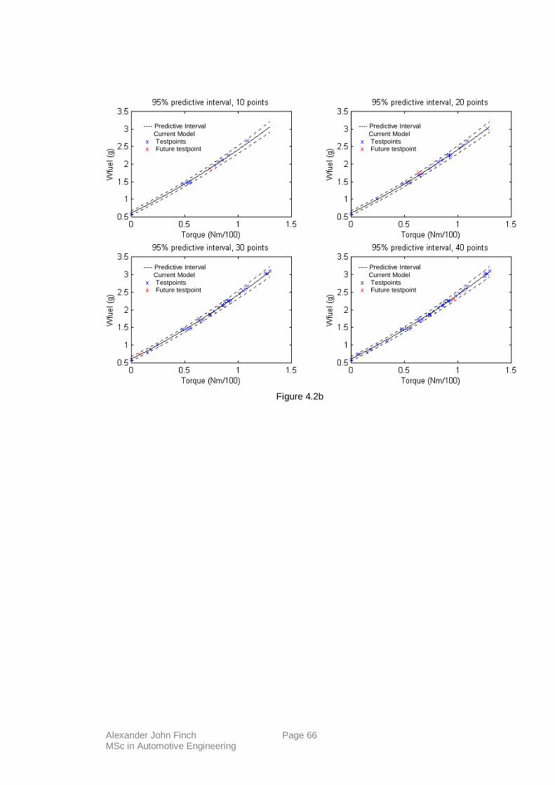
Alexander John Finch Page 66 MSc in Automotive Engineering
Figure 4.2b
---- Predictive Interval �
Current Model x Testpoints x Future testpoint
---- Predictive Interval �
Current Model x Testpoints x Future testpoint
---- Predictive Interval �
Current Model x Testpoints x Future testpoint
---- Predictive Interval �
Current Model x Testpoints x Future testpoint

Alexander John Finch Page 67 MSc in Automotive Engineering
4.24 Effect of model variance on P.I.’s. One variable.
Here we attempt to answer the question: - What effect does assuming the wrong model
variance have on predictive intervals?
The same function, a prior of { 0 | 100 } and model variance of 1e-3 were used.
Assumed model variances of 1e-4, 1e-2 and 1e-1 were used to calculate predictive intervals
after 40 testpoints and the results are shown in figures 4.2c, 4.2d and 4.2e respectively.
Figure 4.2c
---- Predictive Interval �
Current Model x Testpoints x Future testpoint

Alexander John Finch Page 68 MSc in Automotive Engineering
Where the model variance is underestimated we are much more likely to falsely detect outliers.
In fact figure 4.2c shows an outlier wrongly detected at torque = 0.65 – the red cross.
Figure 4.2e
Figure 4.2d
---- Predictive Interval �
Current Model x Testpoints x Future testpoint
---- Predictive Interval �
Current Model x Testpoints x Future testpoint

Alexander John Finch Page 69 MSc in Automotive Engineering
Where the model variance is overestimated outlier detection is limited as the intervals become
wider unnecessarily.
As with confidence intervals, the way to overcome this problem is to give the model variance a
distribution so that it may vary as well.
4.25 Effect of prior knowledge on P.I.’s using functions as datasets. Two variables.
Using the function
Wfuel = 2.05 – 11.13*Eng – 19.5 Torque + 29.01*Eng2 + 55.89*Torque2 + 271.15*Eng*Torque,
prior knowledge { 0, 0, 0, 0, 0, 0 | 10, 1e2, 1e2, 1e3, 1e3, 1e3 } and Model variance �2 = 0.827.
40 testpoints were sampled.
Figure 4.2f shows the observed predictive intervals: -
The interval clearly narrows as more testpoints are sampled since we have increased
information of the model parameters.
With good prior knowledge, { 0, -10, 20, 30, 50, 250 | 10, 10, 10, 10, 10, 100 }. The following
plots are observed.
Predictive Interval
Current Model
Future testpoint
Predictive Interval
Current ModelFuture testpoint
Figure 4.2f

Alexander John Finch Page 70 MSc in Automotive Engineering
Here the predictive interval starts off quite narrow and stays the same as testpoints are added.
i.e testpoints give no extra information.
Figure 4.2g
Current Model
Predictive Interval
Future testpoint

Alexander John Finch Page 71 MSc in Automotive Engineering
4.26 Effect of model variance on P.I.’s. Two variables.
Using a prior of { 0, 0, 0, 0, 0, 0 | 10, 1e2, 1e2, 1e3, 1e3, 1e3 } and sampling data using a
model variance of 0.827, predictive intervals were constructed for various different assumed
model variances.
Figures 4.2h, 4.2i and 4.2j show predictive intervals for assumed model variances of 0.0827,
8.27 and 82.7 respectively. 40 testpoints have been sampled.
Figure 4.2h
Predictive Interval
Current Model
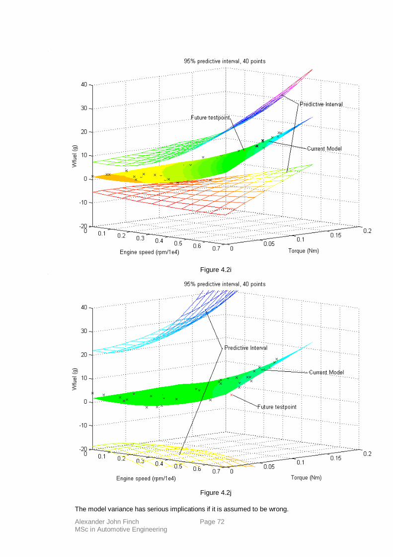
Alexander John Finch Page 72 MSc in Automotive Engineering
The model variance has serious implications if it is assumed to be wrong.
Figure 4.2i
Figure 4.2j
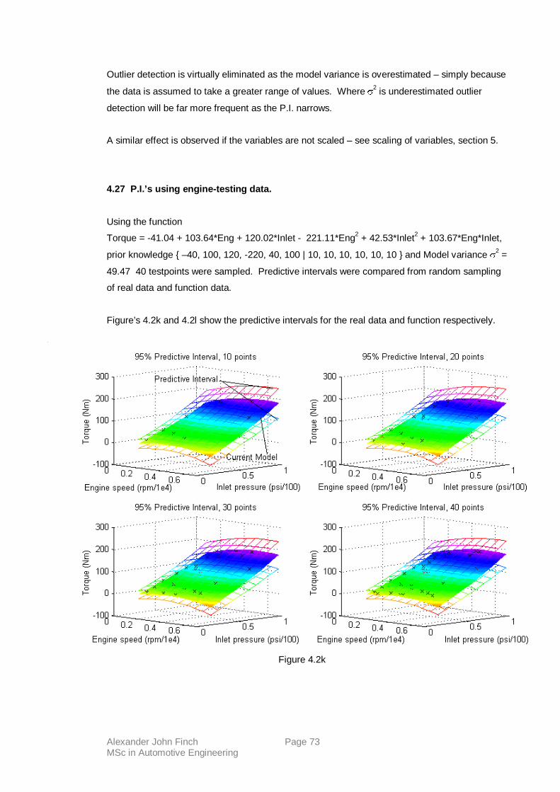
Alexander John Finch Page 73 MSc in Automotive Engineering
Outlier detection is virtually eliminated as the model variance is overestimated – simply because
the data is assumed to take a greater range of values. Where �2 is underestimated outlier
detection will be far more frequent as the P.I. narrows.
A similar effect is observed if the variables are not scaled – see scaling of variables, section 5.
4.27 P.I.’s using engine-testing data.
Using the function
Torque = -41.04 + 103.64*Eng + 120.02*Inlet - 221.11*Eng2 + 42.53*Inlet2 + 103.67*Eng*Inlet,
prior knowledge { –40, 100, 120, -220, 40, 100 | 10, 10, 10, 10, 10, 10 } and Model variance �2 =
49.47 40 testpoints were sampled. Predictive intervals were compared from random sampling
of real data and function data.
Figure’s 4.2k and 4.2l show the predictive intervals for the real data and function respectively.
Figure 4.2k
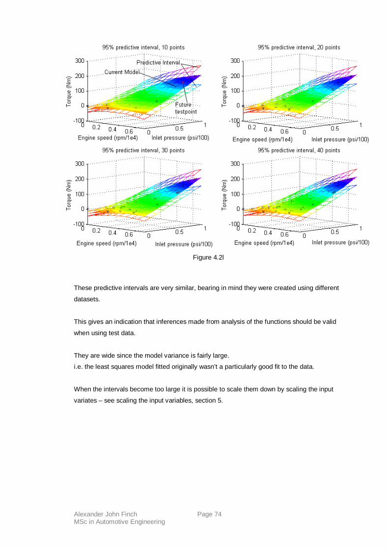
Alexander John Finch Page 74 MSc in Automotive Engineering
These predictive intervals are very similar, bearing in mind they were created using different
datasets.
This gives an indication that inferences made from analysis of the functions should be valid
when using test data.
They are wide since the model variance is fairly large.
i.e. the least squares model fitted originally wasn’t a particularly good fit to the data.
When the intervals become too large it is possible to scale them down by scaling the input
variates – see scaling the input variables, section 5.
Figure 4.2l

Alexander John Finch Page 75 MSc in Automotive Engineering
4.28 Conclusions
The predictive interval is used to find outlying data points. It can achieve this successfully if the
model variance is known precisely. Outlying data points can either be unlikely data points or
possible faults with measuring equipment.
Where the model variance is underestimated outliers can be falsely detected wasting testing
time.
When the model variance is overestimated outlier detection is limited due to the wide predictive
intervals.
Good prior information causes the predictive interval to narrow making it better at detecting
outliers earlier in the testing program. I.e. a narrower interval is created more quickly.
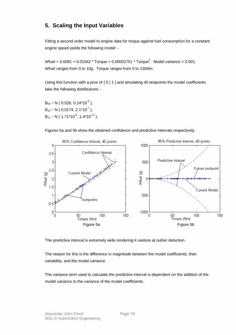
Alexander John Finch Page 76 MSc in Automotive Engineering
5. Scaling the Input Variables
Fitting a second order model to engine data for torque against fuel consumption for a constant
engine speed yields the following model: -
Wfuel = 0.6081 + 0.01542 * Torque + 0.00002751 * Torque2. Model variance = 0.001.
Wfuel ranges from 0 to 10g. Torque ranges from 0 to 130Nm.
Using this function with a prior of { 0 | 1 } and simulating 40 testpoints the model coefficients
take the following distributions: -
B00 ~ N ( 0.526, 0.14*10-3 ),
B10 ~ N ( 0.0174, 2.1*10-7 ),
B11 ~ N ( 1.71*10-5, 1.4*10-11 ).
Figures 5a and 5b show the obtained confidence and predictive intervals respectively.
The predictive interval is extremely wide rendering it useless at outlier detection.
The reason for this is the difference in magnitude between the model coefficients, their
variability, and the model variance.
The variance term used to calculate the predictive interval is dependent on the addition of the
model variance to the variance of the model coefficients.
Figure 5a Figure 5b

Alexander John Finch Page 77 MSc in Automotive Engineering
Consider the 95% predictive interval for a single model coefficient �11: -
= 0.0000171 � 0.062
= ( -0.062, 0.062 )
The variance of �11 has no influence on the predictive interval. The interval is entirely
determined by the model variance. i.e. 1.96*� = 0.062.
In a similar way, when the predictive interval for the model is calculated these differences in
magnitude cause the interval to be much wider than it should be.
Scaling the data before the model is calculated offers a way round this problem since it changes
the values of both the model coefficients and their variances.
For example, in the model above, if torque is scaled down by a factor of 100, torque = torque /
100 – then to maintain the same value of response the model coefficients must increase.
The new model becomes: - Wfuel = 0.6081 + 1.5425 * torque + 0.2751 * torque2.
N.B. Note that the model variance remains the same – see section 1.62.
Using this function and sampling 40 testpoints yields the following model parameters and
variances: -
B00 ~ N (0.7517, 0.1*10-3 ),
B10 ~ N (0.8946, 0.54*10-3 ),
B11 ~ N (0.7094, 0.32*10-3 ).
� � � �����
�� � ������
11
22
1111
22
11*96.1,*96.1 ss
� �001.0140000000000.0*96.10000171.0,001.0140000000000.0*96.10000171.0 ��
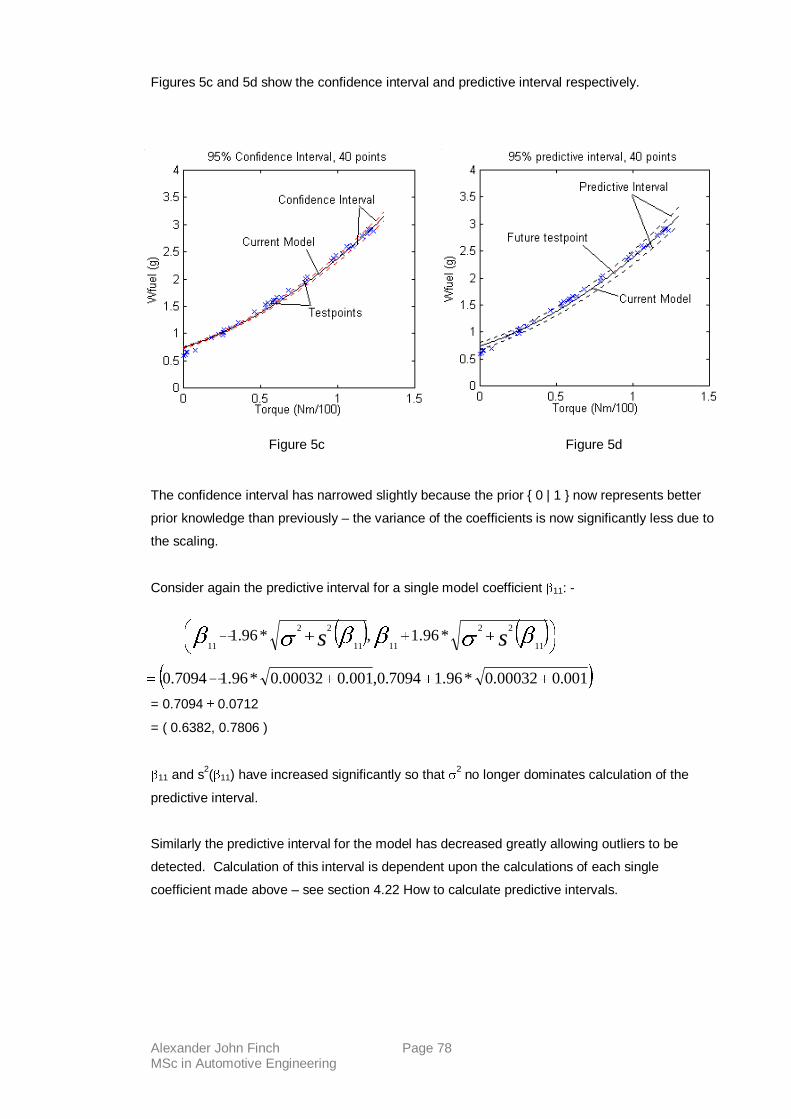
Alexander John Finch Page 78 MSc in Automotive Engineering
Figures 5c and 5d show the confidence interval and predictive interval respectively.
The confidence interval has narrowed slightly because the prior { 0 | 1 } now represents better
prior knowledge than previously – the variance of the coefficients is now significantly less due to
the scaling.
Consider again the predictive interval for a single model coefficient �11: -
= 0.7094 � 0.0712
= ( 0.6382, 0.7806 )
�11 and s2(�11) have increased significantly so that �2 no longer dominates calculation of the
predictive interval.
Similarly the predictive interval for the model has decreased greatly allowing outliers to be
detected. Calculation of this interval is dependent upon the calculations of each single
coefficient made above – see section 4.22 How to calculate predictive intervals.
� � � �����
�� � ������
11
22
1111
22
11*96.1,*96.1 ss
� �001.000032.0*96.17094.0,001.000032.0*96.17094.0 �����
Figure 5c Figure 5d

Alexander John Finch Page 79 MSc in Automotive Engineering
6. Testpoint Selection Methods.
6.1 Why select testpoints?
One of the model assumptions is that the errors are independent of each other. To achieve this
randomisation of the data selection is normally employed.
In frequentist statistics the model is formed after the data have been sampled. So although we
can choose which testpoints to take prior to testing, this would only be based on our knowledge
of the system prior to testing.
Somewhere in this pre selected data set must lie a degree of randomisation for the model to
remain valid. Sometimes the data is split into blocks and then randomised within each block.
Since Bayesian statistics offers us the chance to continuously update our model it is possible to
select testpoints one at a time and analyse the effect they have on the model. In this way
information from each testpoint can be maximised. In the case of engine testing we might be
more interested in one particular area of a range of data and so choose to concentrate testing
there.
Care must be taken though to introduce a degree of randomisation or inferences made from the
model may be invalid. So while we may choose to concentrate testing within a subset of a
particular range it is important to maintain a degree of randomisation.
Traditional engine calibration follows a fixed data selection procedure where testpoints are
selected incrementally from a range of data. The lack of randomisation here may invalidate the
model assumptions.
Alexander John Finch Page 80 MSc in Automotive Engineering
6.2 Selection procedures.
Three selection procedures were tested for their effect on convergence time: -
1. Random.
2. Maximum Residual.
3. Sequential.
1. Random selection was used to compare statistically ideal data selection to possible
preferable techniques.
2. Maximum Residual selection takes testpoints from areas of the model where the residuals
are greatest – i.e. where the difference between the fitted model and the selected data was
greatest. The idea was to try and minimise the largest residual by pulling the model
towards another testpoint nearby.
Preliminary tests showed that choosing the maximum residual each time meant that the
same testpoint would be sampled continuously. In order that some randomisation could be
achieved it was decided that data would be sampled from a normal distribution with a mean
centred on the maximum residual. The 95% range of the distribution was taken as a
proportion of total range of the data. i.e the most likely single value to occur was the
maximum residual.
3. Sequential selection was designed to imitate traditional data selection by taking testpoints
from a pre-determined sequence.

Alexander John Finch Page 81 MSc in Automotive Engineering
6.3 Convergence comparisons.
6.31 One variable.
Using the function: -
Wfuel = 0.6081 + 1.5425 + Torque + 0.2751*Torque2, prior knowledge { 0 | 10 } and �2 = 1e-3 a
comparison of random selection with maximum residual selection was performed.
Table 6.31a compares convergence times for 10 samples of both methods using convergence
criteria of 0.2% over a range of 0 to 1.3.
Selection Method Convergence times
Random 45,44,36,47,35,32,38,58,35,36
Maximum Residual 34,46,45,48,44,61,32,43,47,35
Table 6.31a
Statistical tests show that there is no significant difference between the sizes of these samples.
Figures 6.31a and 6.31b show the models obtained using random and maximum residual
selection respectively.
Figure 6.31a

Alexander John Finch Page 82 MSc in Automotive Engineering
Both models fit the data well but the maximum residual selection seems to diverge from the
sampling function near the end of the range.
Figure 6.31c of the sampling function, estimated model and testpoints shows that data from the
end of the range has not been sampled.
Figure 6.31b
Figure 6.31c

Alexander John Finch Page 83 MSc in Automotive Engineering
Previously it was shown that data sampled directly from a function without added error provided
much clearer differences in convergence whilst reaching the same conclusions. For this reason
the remainder of tests were implemented with no added error to the function.
To compare sequential selection with the other methods, data were selected from a pre-
determined number of points over the range of the data. The initial value of torque = 0.
Where convergence failed to occur after the end of the range had been reached testpoints were
selected at random.
Table 6.31b compares convergence times for different numbers of points.
Number of points to cover
range.
Convergence time.
(Number of testpoints)
Number of random points
selected.
10 38 28
20 45 25
30 47 17
40 50 10
50 58 8
60 66 6
70 74 4
80 78 0
90 81 0
100 84 0
110 86 0
120 88 0
130 88 0
140 87 0
150 65 0
Table 6.31b
Figure 6.31d shows how the convergence times vary with the size of the initial sweep.

Alexander John Finch Page 84 MSc in Automotive Engineering
Convergence times are increasing with the number of testpoints taken to cover the range.
When the number of points reaches 150 convergence is premature - see figure 6.31e.
Figure 6.31d
Figure 6.31e

Alexander John Finch Page 85 MSc in Automotive Engineering
It’s clear from figure 6.31d that the fewer points taken to cover the range initially the less time it
takes to converge. Likewise, the more points chosen at random the less time it takes to
converge.
Is it the number of random testpoints or the size of the initial sweep that makes for quicker
convergence?
Covering the whole range more quickly leaves less scope for the model parameters to change
significantly. Hence convergence is quicker.
In terms of convergence it makes sense to make a sweep of the data first and then to select
data. Even if the first ten data points are fixed they can still be selected at random from within
the group.
Table 6.31c shows convergence times for various initial sweeps followed by maximum residual
searches.
Number of points in initial sweep. Convergence times.
(Number of testpoints)
2 32, 48, 35, 37, 37
3 33, 31, 33, 36, 32
4 34, 35, 35, 36, 34
5 34, 35, 36, 35, 32
10 41, 39, 39, 37, 38
20 44, 43, 43, 44, 44
30 48, 48, 46, 47, 47
40 49, 50, 50, 49, 50
50 58, 57, 58, 58, 58
Table 6.31c
Comparing the values for initial sweeps of 10, 20, 30, 40 and 50 with those from table 6.31b
there appears to be no difference between random selection and maximum residual selection.
What is clear though is that taking an initial sweep containing 2,3,4 or 5 points yields
significantly quicker convergence. Convergence times using these initial sweeps are far more
consistent and smaller compared to convergence times using random or maximum residual
selection only.

Alexander John Finch Page 86 MSc in Automotive Engineering
Is there a significant difference between initial sweep then random selection and initial sweep
then maximum residual selection?
Since the sampling function is somewhat straight over the current range, to compare these
techniques the function y = 0.5+ 8x – 5x2 was used. This function is a bit more ‘curvy’ and will
produce larger changes in the model coefficients as data is sampled.
Table 6.31d compares the techniques over a range of initial sweeps. Prior information was
taken as { 0, 0, 0 | 10, 100, 100 }.
Technique A. Initial sweep then maximum residual selection.
Technique B. Initial sweep then random selection.
Technique Testpoints in
initial sweep
Convergence times.
A 2 42, 36, 38, 46, 47, 42, 40, 40, 47, 38
B 39, 37, 35, 37, 38, 36, 40, 39, 38, 35
A 3 39, 37, 37, 37, 37, 37, 36, 37, 37, 38
B 37, 36, 37, 36, 37, 36, 37, 38, 37, 37
A 4 38, 39, 40, 39, 39, 38, 38, 37, 38, 38
B 38, 39, 38, 38, 38, 38, 38, 39, 38, 39
A 5 40, 40, 40, 39, 41, 39, 39, 39, 40, 39
B 40, 40, 40, 39, 40, 40, 40, 41, 40, 39
A 10 47, 47, 47, 46, 46, 46, 47, 46, 47, 45
B 46, 45, 46, 46, 47, 46, 47, 47, 46, 46
A 20 55, 55, 55, 54, 55, 55, 55, 55, 55, 54
B 55, 55, 55, 55, 55, 55, 55, 55, 55, 54
A 30 61, 61, 61, 60, 60, 61, 60, 61, 60, 61
B 61, 60, 61, 61, 60, 61, 61, 60, 61, 60
Table 6.31d
Figure 6.31f compares the techniques above by plotting the mean convergence times for each
technique.

Alexander John Finch Page 87 MSc in Automotive Engineering
For an initial sweep of two testpoints technique B is more consistent than technique A.
Otherwise convergence times are almost identical. Therefore an initial sweep then random
selection is preferred since it is easier to program and more consistent with the model
assumptions.
The results also suggest that an initial sweep of three testpoints is the optimum value for
quickest convergence.
Figure 6.31f

Alexander John Finch Page 88 MSc in Automotive Engineering
6.32 Two variables.
Using the function
Torque = -41.04 + 103.64*Eng + 120.02*Inlet - 221.11*Eng2 + 42.53*Inlet2 + 103.67*Eng*Inlet,
prior knowledge { 0 | 1e3 } and Model variance = 49.47 the techniques were compared.
The initial sweep this time consisted of a square grid of data.
Table 6.32a compares the techniques.
Technique Testpoints in
initial sweep
Convergence times.
A 4 58, 58, 55, 59, 58, 60, 53, 56, 57, 64
B 60, 61, 60, 57, 59, 56, 58, 57, 58, 58
A 9 55, 54, 54, 54, 54, 54, 55, 54, 54, 54
B 55, 54, 54, 54, 54, 54, 55, 55, 55, 53
A 16 60, 59, 60, 60, 60, 60, 60, 60, 60, 60
B 60, 60, 60, 60, 60, 60, 60, 60, 60, 60
A 25 66, 67, 66, 66, 66, 66, 66, 66, 66, 66
B 66, 67, 66, 66, 66, 67, 66, 66, 67, 66
A 36 72, 73, 72, 72, 72, 72, 72, 72, 72, 72
B 72, 72, 72, 71, 73, 73, 73, 73, 72, 72
A 49 79, 78, 79, 79, 78, 79, 79, 79, 79, 79
B 79, 78, 78, 78, 79, 79, 79, 79, 79, 79
A 64 84, 84, 84, 84, 84, 84, 84, 84, 84, 84
B 84, 84, 84, 84, 84, 84, 84, 84, 84, 84
A 81 89, 89, 88, 89, 89, 89, 89, 89, 89, 89
B 89, 89, 89, 89, 89, 89, 89, 89, 89, 89
A 100 92, 92, 92, 92, 92, 92, 92, 92, 92, 92
B 92, 92, 92, 92, 92, 92, 92, 92, 92, 92
Table 6.32a

Alexander John Finch Page 89 MSc in Automotive Engineering
Figure 6.32a compares the techniques above by plotting the mean convergence times.
Here there is no difference between the techniques. We therefore select the random technique
as the one easiest to implement and most consistent with the model assumptions.
The optimum number of points is nine, i.e. a 3 by 3 grid.
Conjecture: The optimum number of points for convergence of a second order model is 3n
where n is the number of input variables.
Figure 6.32a

Alexander John Finch Page 90 MSc in Automotive Engineering
6.4 Conclusions
An initial sweep of the range of data followed by random selection of testpoints provides both
consistent convergence and valid models.
Where the number of input variables is 1, three evenly spaced points provide quickest
convergence.
Where the number of input variables is 2, nine evenly spaced points provide quickest
convergence.
There are of course many other reasons other than convergence why we might want to select
testpoints. For example – if during testing an area of interest is identified, low emissions, fuel
consumption etc, testing could be stopped and data from that area used again. Either by fitting
a model and creating a new prior or used to update an alternative prior.
Another option would be to run simultaneous models – one of the full range of the input
variables and another of the section of interest. Testing need not stop in this scenario.
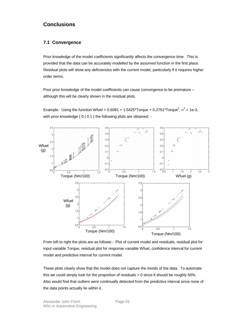
Alexander John Finch Page 91 MSc in Automotive Engineering
Conclusions
7.1 Convergence
Prior knowledge of the model coefficients significantly affects the convergence time. This is
provided that the data can be accurately modelled by the assumed function in the first place.
Residual plots will show any deficiencies with the current model, particularly if it requires higher
order terms.
Poor prior knowledge of the model coefficients can cause convergence to be premature –
although this will be clearly shown in the residual plots.
Example. Using the function Wfuel = 0.6081 + 1.5425*Torque + 0.2751*Torque2, �2 = 1e-3,
with prior knowledge { 0 | 0.1 } the following plots are obtained: -
From left to right the plots are as follows:- Plot of current model and residuals, residual plot for
input variable Torque, residual plot for response variable Wfuel, confidence interval for current
model and predictive interval for current model.
These plots clearly show that the model does not capture the trends of the data. To automate
this we could simply look for the proportion of residuals > 0 since it should be roughly 50%.
Also would find that outliers were continually detected from the predictive interval since none of
the data points actually lie within it.
Torque (Nm/100) Torque (Nm/100)
Torque (Nm/100) Torque (Nm/100) Wfuel (g)
Wfuel (g)
Wfuel (g)

Alexander John Finch Page 92 MSc in Automotive Engineering
Good prior knowledge of the model coefficients gives quicker convergence, although if the prior
variance for the coefficients is too small it is possible to patterns in the residual plots.
Convergence times are not affected by the prior variance for the model coefficients. This is
useful since we have seen that greater prior variances give more consistent convergence –
allowing the data greater influence on the model coefficients.
Modelling higher order systems with lower order functions does not offer any advantage in
terms of convergence time. Prior information in this case can only be of the lower order system
and hence is poor by definition.
Data selection can also effect the convergence time. It was found that an initial sweep of the
range of data followed by random selection provided the quickest and most consistent
convergence. For 1 input variable an initial sweep of 3 points provides quickest convergence.
For 2 input variables an initial sweep of a 3*3 grid of data provides quickest convegence.
It is conjectured that for n input variables an initial sweep of 3n points provides quickest
convergence.
The convergence criteria developed can enable automation to be realised. As the convergence
criteria get tighter the models take longer to converge and vice versa. Further testing needs to
be carried out to assess which convergence criteria provide the best balance of minimum
number of testpoints against the quality of the fitted model.
7.2 Confidence Intervals
Confidence Intervals can be used as a method of assessing the quality of the current model.
The narrower they are the more confidence we have in our fitted model.
They could also be used as a method of assessing convergence of the model. Good prior
information creates smaller confidence intervals earlier in the testing program and hence
quicker convergence. Large model variances place restrictions on the minimum width of the
interval so a specified convergence criteria might never be reached.
Confidence Intervals are highly dependent on knowing the model variance accurately. If the
model variance is underestimated then we can be overconfident with the model. When it is
overestimated then we have less confidence in the model. This problem can be alleviated by
giving the model variance a probability distribution so that it may vary as data is collected.

Alexander John Finch Page 93 MSc in Automotive Engineering
7.2 Predictive Intervals
Predictive Intervals can be used to find outlying data points provided the model variance is
known precisely.
As with Confidence Intervals this can be overcome by giving the model variance a probability
distribution.
Good prior information creates narrower predictive intervals earlier in the testing program and
hence it can detect outliers and possible faults with the measurement equipment more quickly.
7.2 Overall
Bayesian statistical methods will provide a useful tool to enable quicker calibration of engines.
There is not much point in applying this technique if no prior knowledge of the system is
available as this is more likely to hinder the modelling process.
The best technique for testpoint selection – in terms of convergence time - seems to be one of
an initial sweep followed by random selection of testpoints. This requires no input from the
operator and hence can be used for automation purposes.
The Bayesian technique can be used as an adaptive testpoint selection program. I.e. areas of
interest can be identified and testing concentrated. This can invalidate many model
assumptions, particularly one of independent errors. In this case testing could continue using
only data from the range of interest and the current model as a new prior distribution.
Where good prior knowledge of the system is available then areas of interest have presumably
been identified previously and the initial sweep then random selection technique is preferred.
The key to the whole process is knowledge that the data will be well fitted by the chosen model.
This means that the model variance will be small, convergence will be quicker, confidence and
predictive intervals tighter and outliers detected more quickly. Good prior knowledge is then
much more useful in reducing the convergence time.
From the limited data available, second order functions seem to model data from variables such
as torque, engine speed, fuel consumption and inlet pressure effectively. However fitting
second order functions to emissions data is not recommended for use with this technique. They
are clearly of a higher order and may not even be effectively modelled by general linear models.

Alexander John Finch Page 94 MSc in Automotive Engineering
For example the following plots show a second and sixth order model fitted to data for engine
speed and torque against NOx respectively.
Clearly the higher order model is a better fit but still significantly underestimates the response at
many points.

Alexander John Finch Page 95 MSc in Automotive Engineering
The model variance associated with the first plot is 3.7*104. The sixth order model has a model
variance of 2.7*104.
So even though it looks as though it is a lot better the higher order model is still a fairly poor fit
to the data.
8. Recommendations
8.3 Second Order Bayesian Models. In terms of convergence it is recommended that an initial sweep of the range of data followed by
random selection of testpoints is recommended.
The Model Variance �2 should be given a distribution to enable confidence intervals and
predictive intervals to be more reliable as model assessment tools – see reference [3].
Second order functions should only be used on data sets for which they are known to be
appropriate. Fitting models to existing engine data should establish suitable variable
combinations.
Scaling of the input variables is required in cases where the model variance is likely to dominate
calculation of the predictive interval.
Examination of the residual plots is probably the most reliable model assessment tool.
8.2 Future Work.
To be able to use the Bayesian method effectively a consistent system of gathering and storing
data needs to be employed. In this way we can maximise available information prior to testing.
Given a set of input variables and a response it should be possible to identify a suitable order
model, previous data to model as a prior distribution, values to define a distribution for the
model variance and a data selection technique to maximise convergence.
When modelling emissions data and other such non-linear data sets it may still be possible to
implement the Bayesian methodology. It might be possible to use a previous engine mapping
as prior information and then adjust the map as engine data is collected. If you think of the
contour plot as a sheet of elastic on which each point is stretched towards the new datapoint
each time by an amount dependent on its distance away.
This could obviously be extended to higher dimensions by using the concept of distance in
these higher dimensions.

Alexander John Finch Page 96 MSc in Automotive Engineering
One definition of distance between two vectors of points x and y in n-dimensional space is
given by: - � � � � � �yxyxyx nn�
222...
2211 .

Alexander John Finch Page 97 MSc in Automotive Engineering
9. References [1] SP Edwards, D P Clarke, A D Pilley, PGE Anderson, M Hopkins The Role Of Statistics in the Engine Development Process IMechE Journal S550: Statistics for Engine Optimisation December 1998 [2] D Mowell, J Willand, P Binder, A Raab Issues Arising from Statistical Engine Testing IMechE Journal S550: Statistics for Engine Optimisation December 1998 [3] D Mowell, D R Robinson, A D Pilley
Bayesian Experimental Design and its Application to Engine Research and Development SAE Paper 961157 1996
[4] D Mowell, D R Robinson, A D Pilley Optimising Engine Performance and Emissions using Bayesian Techniques SAE Paper 971612 1997 [5] D C Montgomery Design and Analysis of Experiments John Wiley and Sons 1991 [6] http://www.faculty.sfasu.edu/f-cobledw/Regression/Lecture6/Lecture6.PDF

Alexander John Finch Page 98 MSc in Automotive Engineering
Appendix I. Initial MATLAB Program % Bayesian model for Second Order Taylor Approximation with Normally % distributed Prior and likelihood. One input variable clear for i=1:10 close; % closes any open figures end disp( ' ' ); sigma = input( 'model variance = ' ); disp( ' ' ); disp( 'you have assumed the following model' ) disp( 'y=B00 + x1B10 + x1^2B11' ); disp( ' ' ); %% Bmatrix = [ B00 B10 B11 ] %% Bmatrix = [ 0 0 0 ]; %% VarBmatrix = [ var(B00) 0 0 % 0 var(B10) 0 % 0 0 var(B11) ] varBmatrix = [ 1 0 0 0 1 0 0 0 1 ]; AL(1)=input( 'Lower range value for X1 = ' ) AU(1)=input( 'Upper range value for X1 = ' ) F1=linspace(AL(1),AU(1),100); % Series of points over the input variable range F2=F1.^2; [s1,s2]=size(F1); G=[ones(1,s2);F1;F2]; % to enable plotting of the current model iterations = input( 'Number of testpoints = ' ) % Number of random testpoints to sample %%%%%%%% FUNCTION PARAMETER COEFFCIENTS IN HERE%%%%%%%%%%%%%%%%%% % PARAMETERS = [ B00 B10 B11 ] PARAMETERS = [ 2.2 11.73 0.26 ]; %%%%%%%%%%%%%%%%%%%%%%%%%%%%%%%%%%%%%%%%%%%%%%%%%%%%%%%%%%%%%%%%%%% for p = 1:iterations % Main loop for calculating the posterior S(p,1)=AL(1)+rand(1)*(AU(1)-AL(1)); % testpoint number p y=PARAMETERS(1) + PARAMETERS(2)*S(p,1) + PARAMETERS(3)*S(p,1)^2; actualvalue(p)=y; %stores the response value X=[ 1, S(p,1), S(p,1)^2 ]; %The X matrix Xt=transpose(X);
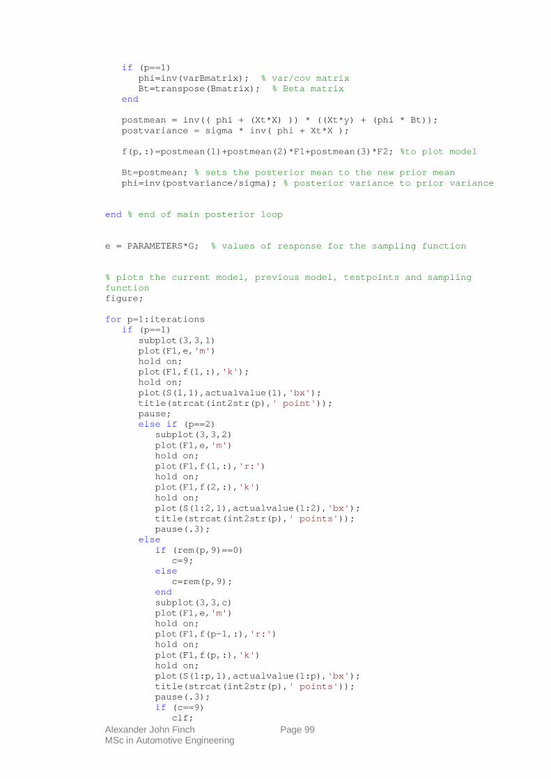
Alexander John Finch Page 99 MSc in Automotive Engineering
if (p==1) phi=inv(varBmatrix); % var/cov matrix Bt=transpose(Bmatrix); % Beta matrix end postmean = inv(( phi + (Xt*X) )) * ((Xt*y) + (phi * Bt)); postvariance = sigma * inv( phi + Xt*X ); f(p,:)=postmean(1)+postmean(2)*F1+postmean(3)*F2; %to plot model Bt=postmean; % sets the posterior mean to the new prior mean phi=inv(postvariance/sigma); % posterior variance to prior variance end % end of main posterior loop e = PARAMETERS*G; % values of response for the sampling function % plots the current model, previous model, testpoints and sampling function figure; for p=1:iterations if (p==1) subplot(3,3,1) plot(F1,e, 'm' ) hold on; plot(F1,f(1,:), 'k' ); hold on; plot(S(1,1),actualvalue(1), 'bx' ); title(strcat(int2str(p), ' point' )); pause; else if (p==2) subplot(3,3,2) plot(F1,e, 'm' ) hold on; plot(F1,f(1,:), 'r:' ) hold on; plot(F1,f(2,:), 'k' ) hold on; plot(S(1:2,1),actualvalue(1:2), 'bx' ); title(strcat(int2str(p), ' points' )); pause(.3); else if (rem(p,9)==0) c=9; else c=rem(p,9); end subplot(3,3,c) plot(F1,e, 'm' ) hold on; plot(F1,f(p-1,:), 'r:' ) hold on; plot(F1,f(p,:), 'k' ) hold on; plot(S(1:p,1),actualvalue(1:p), 'bx' ); title(strcat(int2str(p), ' points' )); pause(.3); if (c==9) clf;

Alexander John Finch Page 100 MSc in Automotive Engineering
end end end end clf; plot(F1,e, 'm' ) hold on; plot(F1,f(p-1,:), 'r:' ) hold on; plot(F1,f(p,:), 'k' ); hold on; plot(S,actualvalue, 'bx' ); title(strcat(int2str(p), ' points' )); postmean postvariance
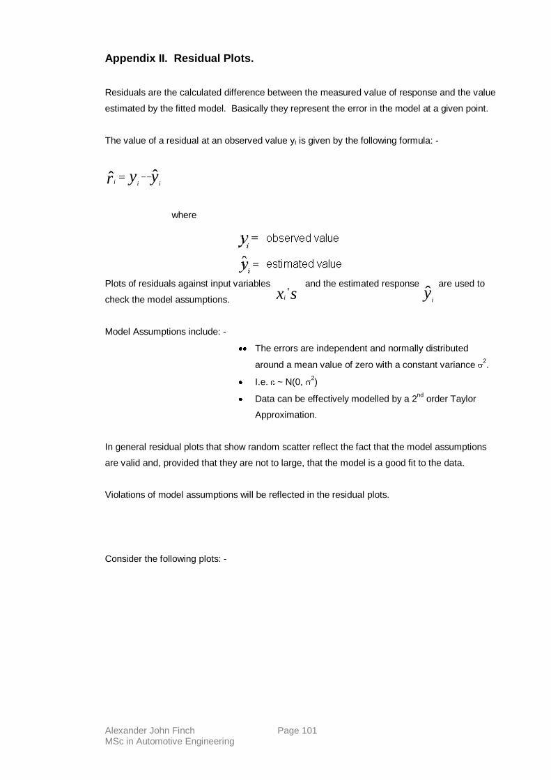
Alexander John Finch Page 101 MSc in Automotive Engineering
Appendix II. Residual Plots.
Residuals are the calculated difference between the measured value of response and the value
estimated by the fitted model. Basically they represent the error in the model at a given point.
The value of a residual at an observed value yI is given by the following formula: -
yyr iii ˆˆ ��
where
Plots of residuals against input variables and the estimated response are used to
check the model assumptions.
Model Assumptions include: -
�� The errors are independent and normally distributed
around a mean value of zero with a constant variance �2.
� I.e. � ~ N(0, �2)
� Data can be effectively modelled by a 2nd order Taylor
Approximation.
In general residual plots that show random scatter reflect the fact that the model assumptions
are valid and, provided that they are not to large, that the model is a good fit to the data.
Violations of model assumptions will be reflected in the residual plots.
Consider the following plots: -
sxi' y
iˆ

Alexander John Finch Page 102 MSc in Automotive Engineering
This sort of pattern indicates that �2 increases with the response variable. In other words the assumption of constant variance is incorrect.
This indicates that the model is missing an xi
3 term.
This is the sort of plot that confirms model assumptions. i.e. nice random scatter over the range.

Alexander John Finch Page 103 MSc in Automotive Engineering
Similarly, any trends observed in the residuals indicates a violation of the model assumptions or
the model is a poor fit to the data.
When such trends are observed reassessment of the model is required.
For example, if residual plots indicate that the model variance increases over the range of data.
Can either give the model variance a probability distribution or transform the response variable
in some way so that the plots appear more random. i.e. use log (yI) instead of yi.

Alexander John Finch Page 104 MSc in Automotive Engineering
Appendix III. Hypothesis Testing.
Consider the following data comparing the heights of flowers grown in two different soils.
Soil Type. Height in cm. Mean. Variance.
I 10.7 11.4 10.0 10.1 11.0 �1= 10.64 s1= 0.2824
II 11.8 10.7 9.4 8.2 11.2 �2= 10.26 s2= 1.6864
From these samples we want to be able to answer questions about the entire population of
flowers grown in each soil.
For instance, “Is there a significant difference in the height of flowers grown in each soil”.
A simple way to measure the difference is to calculate the mean values. �1>�2 so we would
conclude that soil I has taller flowers.
However this test fails to take into account the variability in the samples.
Assuming both samples are normally distributed (a safe assumption for data of this type) then a
plot of the distributions is as follows.
Although the mean for soil II is less there is a much larger variability in the sample giving a
much larger range of plausible values for the mean.
Considering this plot as a distribution for the mean value there is a large area where both
means could be equal, i.e. the overlapping area.

Alexander John Finch Page 105 MSc in Automotive Engineering
We must therefore compare the population of flowers using not only the sample means but the
sample variances as well.
This is achieved using various statistical tests, details can be seen in reference [5] .
In this case, assuming that the population variances are different the following test is applied: -
Calculate t0 =
ns
ns
2
2
2
1
2
1
21
���and v =
12
22
11
21
2
2
1
2
2
2
2
2
1
2
1
�
�
�
�
�
�
�
�
�
�
��
����
���
����
�
nn
s
nn
s
ns
ns
Then t0 < - t�,v � �1<�2
and t0 > t�,v � �1>�2
else �1=�2
These tests are historically taken at an alpha level of 95%.
t�,v is the upper � percentage point of the t-distribution with v degrees of freedom.
The t-distribution is similar to a normal distribution but with fatter tails to account for the
uncertainty associated with an unknown variance.
For the data above t0=0.61, v= 5.3 and t0.95,5.3 � 1.96.
Since 0.61 > -1.96
0.61 < 1.96 we conclude that there is evidence to suggest that the means
are equal.