Embed Size (px)
Citation preview

HAL Id: hal-01786977https://hal.archives-ouvertes.fr/hal-01786977
Submitted on 9 Apr 2020
HAL is a multi-disciplinary open accessarchive for the deposit and dissemination of sci-entific research documents, whether they are pub-lished or not. The documents may come fromteaching and research institutions in France orabroad, or from public or private research centers.
L’archive ouverte pluridisciplinaire HAL, estdestinée au dépôt et à la diffusion de documentsscientifiques de niveau recherche, publiés ou non,émanant des établissements d’enseignement et derecherche français ou étrangers, des laboratoirespublics ou privés.
An approach based on support vector machines and aK-D Tree search algorithm for identification of the
failure domain and safest operating conditions in nuclearsystems
Francesco Di Maio, Alessandro Bandini, Enrico Zio, Andrea Alfonsi, CristianRabiti
To cite this version:Francesco Di Maio, Alessandro Bandini, Enrico Zio, Andrea Alfonsi, Cristian Rabiti. An approachbased on support vector machines and a K-D Tree search algorithm for identification of the failuredomain and safest operating conditions in nuclear systems. Progress in Nuclear Energy, Elsevier, 2016,88, pp.297-309. �10.1016/j.pnucene.2016.01.017�. �hal-01786977�

1
AN APPROACH BASED ON SUPPORT VECTOR MACHINES
AND A K-D TREE SEARCH ALGORITHM FOR
IDENTIFICATION OF THE FAILURE DOMAIN AND SAFEST
OPERATING CONDITIONS IN NUCLEAR SYSTEMS
Francesco Di Maio1, Alessandro Bandini1, Enrico Zio1,2, Alfonsi Andrea3, Cristian Rabiti3
1Energy Department, Politecnico di Milano, Milan, Italy 2 Chair System Science and the Energy Challenge, Fondation Electricite’ de France (EDF),
CentraleSupélec, Université Paris-Saclay, Chatenay-Malabry, France 3Idaho National Laboratory, Idaho Falls (ID), U.S.A.
Corresponding Author: Dr. Francesco Di Maio
Tel: +390223996372, Fax: +390223998566, Email: [email protected]
Abstract
The safety of a Nuclear Power Plant (NPP) is verified by analyzing the system responses under normal
and accidental conditions. This is done by resorting to a Best-Estimate (BE) Thermal-Hydraulic (TH)
code, whose outcomes are compared to given safety thresholds enforced by regulation. This allows
identifying the limit-state function that separates the failure domain from the safe domain.
In practice, the TH model response is affected by uncertainties (both epistemic and aleatory), which
make the limit-state function and the failure domain probabilistic.
The present paper sets forth an innovative approach to identify the failure domain together with the
safest plant operating conditions. The approach relies on the use of Reduced Order Models (ROMs)
and K-D Tree.
The model failure boundary is approximated by Support Vector Machines (SVMs) and, then, projected
onto the space of the controllable variables (i.e., the model inputs that can be manipulated by the plant
operator, such as reactor control-rods position, feed-water flow-rate through the plant primary loops,
accumulator water temperature and pressure, repair times, etc.). The farthest point from the failure
boundary is, then, computed by means of a K-D Tree-based nearest neighbor algorithm; this point
represents the combination of input values corresponding to the safest operating conditions.
The approach is shown to give satisfactory results with reference to one analytical example and one
real case study regarding the Peak Cladding Temperature (PCT) reached in a Boiling Water Reactor
(BWR) during a Station-Black-Out (SBO), simulated using RELAP5-3D.
Keywords: Risk-Informed Safety Margins Characterization; Failure Boundary; Reduced-Order
Models; Support Vector Machines; K-D Tree; Station Black Out Accident.
2
1. INTRODUCTION
The Risk-Informed Safety Margins Characterization (RISMC) pathway of the Light Water
Reactors Sustainability (LWRS) program of the U.S. Department of Energy (DOE) [DOE,
2009] aims at developing decision making methods and tools, for use in the process of licensing
new nuclear technologies and evaluating existing Nuclear Power Plants (NPPs) for lifetime
extension.
One key aspect is the safety assessment, which is performed based on the calculations by a
Thermal-Hydraulic (TH) - neutronic code of the nuclear system response in normal and
accidental conditions. Specific outputs are selected as safety-significant parameters and their
calculated values are compared with some threshold values, in order to check that sufficient
safety margins are kept during accident [Gavrilas et al., 2004].
Traditionally, this safety assessment procedure has been performed on a small set of Design
Basis Accidents (DBAs) and under tight conservative assumptions (i.e., on the phenomena
dynamics described, physical models implemented, etc.) to protect against the uncertainties in the
model and its parameters.
In recent times, an extended and more realistic approach has been undertaken, including
Beyond Design Basis Accidents (BDBAs) and relying on Best Estimate (BE) codes, in which more
realistic assumptions are taken in the evaluation of the safety margins [Zio et al., 2010; Alvarenga
et al., 2015]. Under this setting, an accurate and explicit treatment of the
uncertainties is required, in order to provide confidence that plant safety margins are not
actually reduced [Zio et al., 2008; Apostolakis, 1990; Schuëller et al., 2008].
Such uncertainty quantification has shifted the concept of safety margins to a probabilistic
paradigm, whereby the code outcomes are treated as stochastic variables [Zio et al., 2008;
Schuëller et al., 2008].
Mathematically, a BE-TH code for safety assessment may be seen as an ensemble of three
elements: i) a set of equations coded to describe the system response ii) an n-dimensional input
vector of stochastic variables 1 2, , ,
nX X X X and iii) an o-dimensional output vector of
stochastic variables 1 2, , ,
oY Y Y Y . The input vector X consists of the model parameters and
input variables that feed the coded equations to compute the model output vector Y that
represents the systems response. In mathematical words, a BE-TH code can be seen as the
multidimensional and non-linear operator m that maps the input vector X into the output
vector Y [Bourinet et al., 2011]:
3
Y m X (1)
In general, uncertainties affecting the model outcome may be due to: inherent stochastic
behavior of the process described by the model m (aleatory uncertainty), imperfect knowledge
about the model input variables X and lack of information on the underlying physical
phenomena (epistemic uncertainty) [Apostolakis, 1990; Möeller et al., 2008; Helton et al.,
2011]. Then, mathematically, the input vector X is uncertain and, therefore, the output vector
Y is uncertain as well, with stochastic realizations (in the following, upper case letters are used
to identify stochastic variables and lower case letters are used to identify their realizations, as
usual):
1 2 1 2{ , , , } ( , , , )
o ny y y y m x m x x x (2)
With reference to a plant accident scenario FE (i.e., a sequence of events that can (or not) lead
to system failure) and to a safety threshold yγ of the vector y of safety thresholds, each one
of these not to be exceeded by the respective safety parameter YY , a limit-state function G
can be defined as:
yy γXYγXGG )(),( (3)
The model is in safe operating conditions when 0),( yγXG and fails when 0),( yγXG .
Then, ),( yγXG separates the input variables space n in a safe domain, { : ( , ) 0},
yS X G X γ
and a failure domain, }0),(:{ yγXGXF . The failure probability, i.e. the probability of
occurrence of the plant accident scenario FE is, then, given by:
( , ) 0( ) ( ( , ) 0) ( )
yF y XG X γ
P E P G X γ f x dx
(4)
where )(xfX
is the joint Probability Density Function (PDF) of the stochastic input vector X
[Cadini et al., 2014]. The set of input values 0),(: yγXGX defines the failure boundary F
4
within the input space (i.e., n ), for a given value of the safety threshold yγ . Because the
)( FEP values are low for high-reliable systems (such as NPPs) and the BE-TH models of these
systems are computationally expensive, these latter can be replaced by Reduced Order Models
(ROMs) to allow the estimation of F within a reasonable computational time [Zio et al., 2008;
Chakraborty et al., 2015]. Indeed, ROMs are designed to capture the dominant non-linear
behavior of the BE-TH models based on a simplified mathematical representation [Lucia et al.,
2004].
In this work, the model failure boundary F is approximated by means of a Support Vector
Machines (SVM)-based ROM [Basudhar et al., 2008; Cortes et al., 1995; Guyon et al., 1993]
that is embedded in a K-D Tree-based nearest neighbors search algorithm [Bentley, 1975;
Katayama et al., 2000; Maneewongvatana et al., 2001] to determine the farthest point from F
inside the input space n : this point represents the optimal combination of the model input
values that results in the safest plant operating conditions (farthest from the failure boundary)
with reference to some given safety requirements expressed by yγ . The main advantage of
adopting SVMs lies in their superior ability, with respect to other ROMs (such as Artificial
Neural Networks (ANNs) and simple linear regression models), to define complex decision
functions (i.e., hyper-planes) in a multidimensional space and exploit optimal separating
functions in order to decompose multiple classes of data [Basudhar et al., 2008; Zio et al.,
2012]. On the other hand, the selection of the K-D Tree algorithm as searching algorithm is
motivated by the fact that it helps finding the nearest neighbors faster than other brute-force
searching approaches [Maneewongvatana et al., 2001]. It is worth pointing out that the K-
D Tree algorithm does not requires the SVM to be embedded, but, rather, this can be used
as searching algorithm driven by any other ROM for the definition of F .
Knowledge of the safest plant conditions offers practical benefits as X is comprised of two
different types of inputs: controllable and non-controllable [Mohsine et al., 2010]. The former
identify the levers under control of the plant operator, which can be manipulated to increase
plant safety (i.e., reactor control-rods position, feed-water flow-rate through the plant primary
loops, accumulator-water temperature and pressure, repair times, etc.), whereas the latter define
the random parameters that may (adversely) affect the model response by increasing the
likelihood of an accident (i.e., pipelines friction factors, temperature and pressure of the final
heat-sink, break section equivalent diameter, failure times, etc.). In this respect, it should be
pointed out that were yγ not “a priori” known but, rather, obeying a probability distribution

5
)( yγfy
, the same input vector realization x might imply failure, 0),( yγxg , or success,
0),( yγxg and, thus, the stochastic safety threshold y should be included in the non-
controllable input variables subset [Banks et al., 2011] so that the input space n is expanded
into1 n.
F
)( FEP
Once the controllable variables are identified, we can project the failure boundary on the
controllable variables space so as to draw “first principles” guidelines for counteracting the
incipient plant failure that depends on the occurred accident and the non-controllable variables.
The rest of this paper is organized as follows. Section 2 illustrates the application of SVMs for
the failure boundary estimation. Section 3 shows the approach used to identify the system safest
operating conditions. In Section 4, the proposed approach is applied to an analytical example
used as proof of concept and in Section 5 it is tested on a Loss of Offsite Power (LOOP) case
followed by a Station Black Out (SBO) accident in a Boiling Water Reactor (BWR), whose
behavior is simulated by a RELAP5-3D BE-TH code. In Section 6 conclusions are drawn.
2. FAILURE BOUNDARY ESTIMATION
As already said, simulations for the safety assessment of NPPs are computationally expensive
due to the small values of . As only limited computing resources are generally available,
the investigation of an exhaustive set of simulation outcomes, accounting for all normal and
accidental plant conditions, is impractical. For this reason, this work exploits a combination of
two ROMs to minimize the computational time used to identify F with sufficient accuracy
(as later defined in terms of persistence):
i. a Physical ROM (P-ROM): a SVM regresses the physical model response of the BE-
TH code (see Appendix A for more details on SVMs);
ii. a Boolean ROM (B-ROM): a SVM classifies the P-ROM outputs as belonging either
to the safe or failure domain for the identification of F . It is worth mentioning that the
B-ROM is not built directly on the physical model responses of the BE-TH code but on
the P-ROM responses as this allows speeding-up the B-ROM evaluations by making
G smoother and easier to handle.
We adopt an adaptive sampling algorithm [Rabiti et al., 2014a] for the approximation of the

6
model failure boundary F : i) RN model responses are obtained from the original BE-TH
simulations, ii) a P-ROM is built to capture the general BE-TH model behavior, iii) a few new
input values are sampled and the BE-TH responses are predicted by the P-ROM, iv) a B-ROM
is built to classify the P-ROM outputs as failure or success, iii) new samples are selected based
on the B-ROM constructed, v) the B-ROM is iteratively updated based on the P-ROM
responses to the new sampled points, until F is identified. This iterative algorithm allows
focusing samples on risk-sensitive regions of the input space so that the number of expensive
trials needed to localize the boundary is reduced.
The strategy hereby described to estimate F is implemented in the RAVEN code, within a
project developed by the Idaho National Laboratory (INL) under the Nuclear Energy Advanced
Modeling and Simulation (NEAMS) and Light Water Reactor Sustainability (LWRS)
programs to provide software tools for the enforcement of the Risk Informed Safety Margins
Characterization (RISMC) conceptual framework supported by the U.S. Department of Energy
(DOE) [Rabiti et al., 2014b]. In more detail, the iterative algorithm is comprised of the
following steps (without loss of generality, we consider a random safety threshold y and a
single model output Y ):
1. at the 1 iteration, a limited number 0n of points
)(
21
)2(
21
)1(
210),,,,(,,),,,,(,),,,,(
n
ynynyn γxxxγxxxγxxx is sampled from the 1n
input space through a brute-force approach (i.e., Monte Carlo, grid, stratified sampling,
etc.); The sampled 0n points are, in principle, more than (and different from) the set of
input values that have generated the RN available BE-TH model responses;
2. at each ξ-th iteration, the P-ROM (previously trained on the RN available BE-TH model
responses) is employed to predict )()2()1( 0~,,~,~ nyyy , which reproduce the BE-TH code
responses )()2()1( 0,,,n
yyy to the set of 0n sampled points;
3. a Boolean function ),,,,( 21 yn γxxxzz is evaluated on each pair of points
)(
21
)2(
21
)1(
210)~,,,,,(,,)~,,,,,(,)~,,,,,(
n
ynynyn yγxxxyγxxxyγxxx :
1 2
1 2
1 2
1, ( , , , , ) 0( , , , , )
1, ( , , , , ) 0
n y
n y
n y
G x x x γz z x x x γ
G x x x γ
(5)

7
4. a B-ROM is trained on the0n points and used to predict
)()2()1( ~,,~,~ gnzzz , e.g., the
Boolean responses of ),,,,( 21 yn γxxxz on a new set of gn input values
)(
21
)2(
21
)1(
21 ),,,,(,,),,,,(,),,,,( gn
ynynyn γxxxγxxxγxxx that are sampled on a
regular Cartesian grid in the input space;
5. the failure domain F is defined by the set of input values resulting in a B-ROM
response 1),,,,(~21 yn γxxxz . This allows identifying the failure boundary F as
the set of input values ,),,,,(,),,,,( )2(
21
)1(
21 FynFyn γxxxγxxx that determine the
transition of ),,,,(~21 yn γxxxz from -1 to +1;
6. among points ,),,,,(,),,,,( )2(
21
)1(
21 FynFyn γxxxγxxx , the farthest one from
)(
21
)2(
21
)1(
210),,,,(,,),,,,(,),,,,(
n
ynynyn γxxxγxxxγxxx is added to the 0n training
data and the algorithm is resumed at Step 2. By so doing, the B-ROM is retrained on a
new point in the most risk-sensitive region of the input space (i.e., boundary between
system safe and system failure), which is the farthest from the current training data;
7. a persistence value )( is computed for each φ-th point of F :
)()(
1
)( ~~
zz (6)
If all )( are equal to 0 (i.e., any of the F points have changed) for a pre-defined
number of consecutive iterations: a) new input points are added to the training set to
explore farther regions of the input space from F and b) the process is resumed at Step
2.
When a pre-defined persistence requirement is met, the algorithm stops and F is obtained as
the set of input points of the B-ROM failure domain ( 1),,,,(~21 yn γxxxz ) and safe domain
( 1),,,,(~21 yn γxxxz ), that determine the transition of ),,,,(~
21 yn γxxxz from -1 to +1.
3. SAFEST OPERATING CONDITIONS IDENTIFICATION
In the most general case, some model input variables are controllable (i.e., qXXX ,,, 21 ),

8
while some others are not (i.e., nqq XXX ,,, 21 ). The controllable and non-controllable input
spaces are q and 1 qn , respectively, and the y has been included in the non-controllable
input space as, without loss of generality, we consider the model safety threshold as a random
variable.
The herein proposed approach for the safest operating conditions identification requires in
input:
i. Fthe set of n+1-dimensional points of (that can be estimated as in Section 2, by
resorting to a P-ROM and a B-ROM, that in this case have been chosen to be SVMs for
regression and classification, respectively);
ii. the distributions of the model input variables (i.e., )).(),(,),(),( 21 21 ynXXX γfxfxfxfyn
In particular, the available information on F (shown in Figure 1 for 2n controllable
variables, where dots are safe points ( 1~ z ) and stars are failure points ( 1~ z ) is, then,
manipulated within a K-D Tree algorithm [Bentley, 1975; Katayama et al., 2000;
Maneewongvatana et al., 2001], as follows, for a 31n -dimensional problem with 2q
controllable (21, XX ) and 11 qn non-controllable ( y ) variables.
In general terms, the K-D Tree algorithm is a space-partitioning data structure for organizing
points in a K-Dimensional space [Bentley, 1975]. The K-D tree is a binary tree structure which
recursively partitions the input space along the axes that divide it into nested orthotropic
regions into which data points are filed. This is done to address the computational inefficiencies
of the brute-force Nearest Neighborhood approaches and to reduce the required number of
distance calculations by efficiently encoding aggregate distance information for the sample (the
basic idea is, indeed, that if point A is very distant from point B, and point B is very close to
point C, then, A is distant from C without calculating the distance between A and C). The
construction of a K-D tree is very fast: because partitioning is performed only along the axes,
no D-dimensional distances need to be computed. Rather, when a (2-D) point is assigned to a
node of the tree, the two coordinates are chosen, alternatively, and their medians are calculated
to define horizontal or vertical lines, that, recursively, define areas containing other data that
are classified in the left and right branches thereby departing that are, respectively, on the left
and right of the point corresponding to that node in the 2-D space. Figure 2 shows an intuitive
2-D tree construction for the identification of the nearest safe point to any of the available
safe

9
conditions plotted in Figure 1 (i.e., only X1 and X2 are considered as input variables for the KD
tree construction): the methodological generalization to a higher-dimensional problem is
straightforward [Bentley, 1975].
Figure 1: failure boundary F for 2n controllable input variables (dots are safe points ( 1~ z ) and stars
are failure points ( 1~ z )).
Figure 2: KD tree construction for the identification of the nearest safe point to any of the available safe
conditions plotted in Figure 1.

10
The proposed approach can be summarized as follows:
1. One set of values (i.e., ,,,,,,,,,,, )2()1()2()1()2(
2
)1(
2
)2(
1
)1(
1 yynn γγxxxxxx ) is sampled for each
input variable from its PDF (i.e., )(),(,),(),( 21 21 ynXXX γfxfxfxfyn );
2. the sampled values of the controllable variables (i.e., ,,,,,,,, )2()1()2(
2
)1(
2
)2(
1
)1(
1 qq xxxxxx )
are used to build a q-dimensional grid (hereafter called controllable grid), whereas the
sampled values of the non-controllable variables (i.e.,
,,,,,,,,,,, )2()1()2()1()2(
2
)1(
2
)2(
1
)1(
1 yynnqqqq xxxxxx ) are used to build a n-q+1-dimensional
grid (hereafter called non-controllable grid) (shown in Figure 3 for 2n and 2q );
Figure 3: on the left side, a 2q -dimensional controllable grid; on the right side, a 11 qn -
dimensional non-controllable grid.
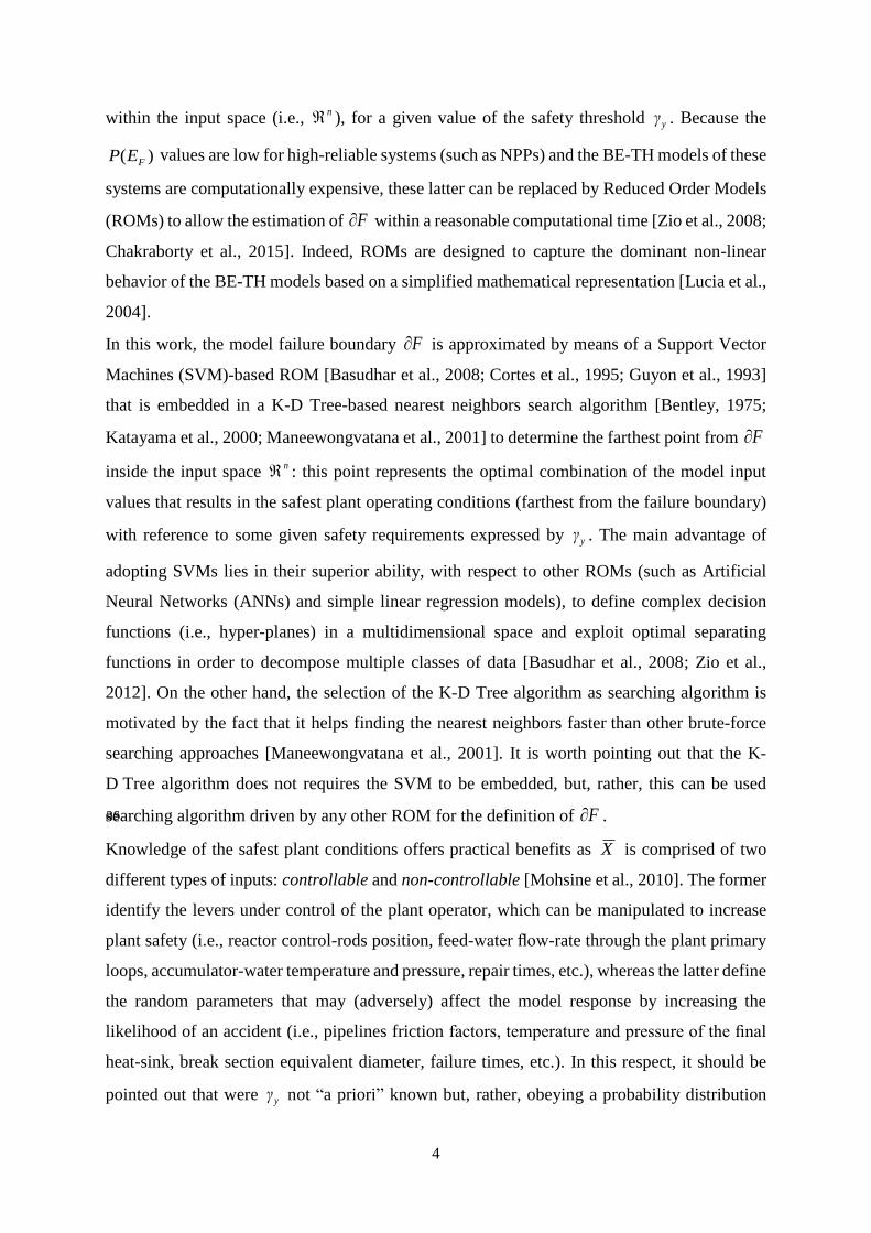
3. an exhaustive list of pairwise combinations ),,,,,,,,( 2121 ynqqq γxxxxxx of the
controllable and non-controllable coordinates is built;
4. for each point )),,,,(,,,,( 2121
ynqqq γxxxxxx belonging to the set of entries
),,,,,,,,( 2121 ynqqq γxxxxxx , which is defined by the same ψ-th set of non-controllable
variables )(
21 ),,,,(
ynqq γxxx , a K-D Tree-based nearest neighbor algorithm is
employed to identify the closest point Fynqqq γxxxxxx ),,,,,,,,( 2121 of F (Figure 4)
for which 1)),,,,,,,,((~2121 Fynqqq γxxxxxxz .
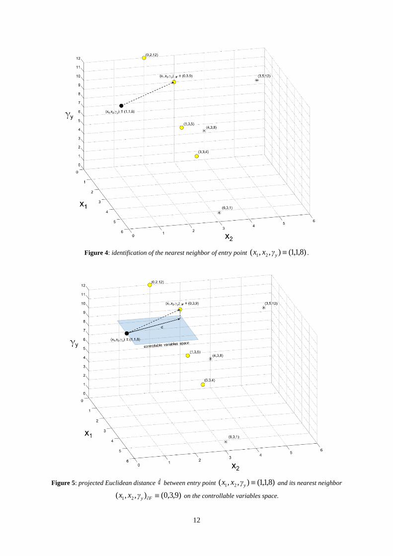
5. the projection d on the controllable input space (i.e., q ) of the Euclidean distance
between ),,,,,,,,( 2121 ynqqq γxxxxxx and Fynqqq γxxxxxx ),,,,,,,,( 2121 is

11
computed (Figure 5);
6. the farthest point )),,,,(|,,,( )(
21
**
2
*
1
*
ynqqq γxxxxxxx in the safe domain S from the
ψ-th projection of F on q is identified, which is the point such that }max{dd In
other words, *
x is the safest point of the controllable input space for the ψ-th set of non-
controllable values )(
21 ),,,,(
ynqq γxxx ;
7. to each*
x one probability value *
P is associated, which is computed as the product of all
the non-controllable variables marginal densities:
)()()()( )()()(
22
)(
11
*
yynnqqqq γPxXPxXPxXPP (7)
8. the absolute safest position *x can be computed as one of the following quantities:
i. mean:
*** xPx (8)
ii. median:
5.0),,,,(: )()()(
22
)(
11
**
yynnqqqq γxXxXxXPxx (9)
iii. α-th percentile:
100),,,,(: )()()(
22
)(
11
** yynnqqqq γxXxXxXPxx (10)
As it is easy to see, both mean and median of the *
x population are solutions based on the
most probable behavior of the non-controllable variables, whereas the α-th percentile defines
a more or less risk-oriented solution depending on and on what non-controllable variables
are actually considered.
12
Figure 4: identification of the nearest neighbor of entry point )8,1,1(),,( 21 yγxx .
Figure 5: projected Euclidean distance d between entry point )8,1,1(),,( 21 yγxx and its nearest neighbor
)9,3,0(),,( 21 Fyγxx on the controllable variables space.

13
4. PROOF OF CONCEPT USING AN ANALYTICAL EXAMPLE
4.1 Analytical Model Description
The proposed approach is tested on an analytical model m , whose mathematical expression is
given as:
3
1
2
21
2
121 )1()2()3(8),( XXXXXXmY (11)
where inputs jX ( 2,1j ) are independent random variables obeying two truncated normal
distributions: 10,101 X ~ )4,2(1N , 10,102 X ~ )25.6,0(1N . The model limit-state
function G can be written as:
yyy XXXXYXGG 3
1
2
21
2
1 )1()2()3(8),( (12)
where the model safety threshold is distributed as a truncated normal variable
2500,500y ~ )2500,500(3N and the model failure boundary is
}0),,(:),,{( 2121 yy XXGXXF .
4.2 Failure Boundary Estimation
The methodological steps described in Section 2 have been applied to model m to obtain the
estimate F~
of the failure boundary, where:
1. an initial training set of 110250 n input points
)(
21
)2(
21
)1(
210),,(,,),,(,),,(
n
yyy γxxγxxγxx is sampled on a regular Cartesian grid
2500:125:50010:1:1010:1:10 ;
2. then, a P-ROM should be trained to reproduce the model m responses )()2()1( 0,,,n
yyy
to the input set of points )(
21
)2(
21
)1(
210),,(,,),,(,),,(
n
yyy γxxγxxγxx . However, in this
particular analytical example considered, the model m of Eq. (11) and the
14
corresponding limit state function G of Eq. (12) are known, so that we resort directly to
Eq. (11) to compute )()2()1( 0,,,n
yyy , instead of training the P-ROM; in other words,
simulation data are directly used through Eq. (12) with a sampled safety limit γy to
identify the set of inputs (x1, x2,..,xn| γy) that are on the limit surface;
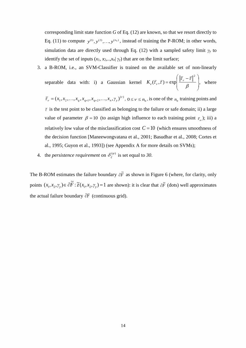
3. a B-ROM, i.e., an SVM-Classifier is trained on the available set of non-linearly
separable data with: i) a Gaussian kernel
2
exp),(eK , where
)(
2121 ),,,,,,,,(
ynqqq γxxxxxx , 00 n , is one of the
0n training points and
is the test point to be classified as belonging to the failure or safe domain; ii) a large
value of parameter 10 (to assign high influence to each training point ); iii) a
relatively low value of the misclassification cost 10C (which ensures smoothness of
the decision function [Maneewongvatana et al., 2001; Basudhar et al., 2008; Cortes et
al., 1995; Guyon et al., 1993]) (see Appendix A for more details on SVMs);
4. the persistence requirement on )(
is set equal to 30.
The B-ROM estimates the failure boundary F~
as shown in Figure 6 (where, for clarity, only
points 1),,(~:~
),,( 2121 yy γxxzFγxx are shown): it is clear that F~
(dots) well approximates
the actual failure boundary F (continuous grid).

15
Figure 6: plot of the estimated F~
(i.e., dots) and of the actual failure boundary F (i.e., continuous grid) for
the analytical model h considered.
For the case of interest, inputs jX ( 2,1j ) are considered the model controllable variables
and y is the only non-controllable variable. Accordingly, the controllable and non-
controllable input spaces are 10,1010,10 and 2500,500 , respectively.
The model absolute safest operating conditions *x will be given as pairwise combinations of
1X and 2X values (i.e., points in the controllable space 10,1010,10 ), while )( yγf
y
will be exploited to assign a *
P probability value to each relative safest operating condition
*
x (as shown in detail in Sections 3, Steps from 2 to 7).
4.3 Safest Operating Conditions Identification
In order to identify the safest operating conditions *x of the system whose behavior is modeled
by m , the approach proposed in Section 3 has been enforced on the failure boundary F~
estimated in Section 4.2.
The controllable and non-controllable grids are built on a Cartesian grid (i.e.,

16
2500:125:50010:5.0:1010:5.0:10 ). For each sampled value of y one
projection of F~
is obtained on the controllable input space 10,1010,10 and one
relative safest position *
x is computed.
Figure 7 shows that: i) the ψ-th projection F~
of the estimated failure domain F~
changes in
size and shape with y (i.e., as y increases F~
decreases as shown in Figure 8 ), ii) *
x
changes its position in the controllable input space as F~
changes (Figure 8), iii) different
statistical quantities (i.e., mean, median, 20-th and 80-th percentiles) derived from the
population of *
x (the relative safest operating conditions for each ψ-th set of non-controllable
variables) and their associated *
P values result in different positions for *x (the safest
operating conditions) in the controllable input space.
In particular, it is worthwhile considering that when the system is operated under very stressful
conditions (i.e., system response Y is allowed to approach y upper limit) as y is set equal
to its 99-th percentile, for instance, the relative safest point *
x might actually be localized
within a failure region defined for conservative conditions, i.e., for small values of y (Figure
7).
For this reason, different strategies should be defined to help the plant operator decide on what
safest operating condition *x to select depending his/her attitude towards risk:
i. risk-averse: *x is chosen as the 20-th percentile of the *
x population, which amounts
to the safest operating conditions when the system is working under very conservative
hypothesis (Y is kept far below the upper limit of y );
ii. risk-prone: *x is the 80-th percentile of the *
x population, which is the safest operating
conditions determined for the system functioning in extreme conditions (Y is allowed
getting close to y upper limit);
iii. mean/median: both strategies aim at identifying *x based on the average behavior of
y .
17
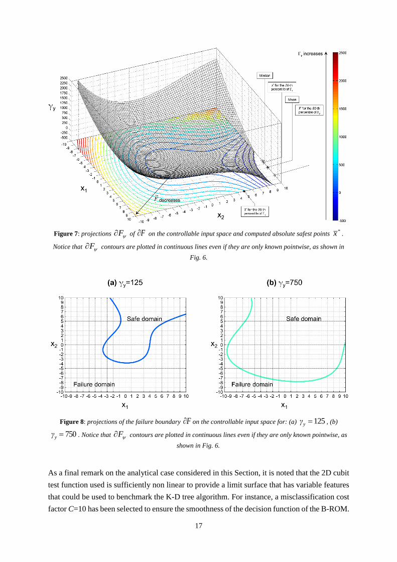
Figure 7: projections F of F on the controllable input space and computed absolute safest points*x .
Notice that F contours are plotted in continuous lines even if they are only known pointwise, as shown in
Fig. 6.
Figure 8: projections of the failure boundary F on the controllable input space for: (a) 125yγ , (b)
750yγ . Notice that F contours are plotted in continuous lines even if they are only known pointwise, as
shown in Fig. 6.
As a final remark on the analytical case considered in this Section, it is noted that the 2D cubit
test function used is sufficiently non linear to provide a limit surface that has variable features
that could be used to benchmark the K-D tree algorithm. For instance, a misclassification cost
factor C=10 has been selected to ensure the smoothness of the decision function of the B-ROM.

18
To test the smoothness (or lack of overfitting) of the B-ROM, a random noise variable can be
added to Eq. (11) and the analysis can be performed on several training sets with varying
magnitudes of the noise variance. If the B-ROM is robust, the limit surface shown in Figure 6
should be insensitive to random noise. However, the demonstration that the training of the B-
ROM is robust to random noise and that overfitting can be avoided is not the scope of the work,
while it can be found in the literature [Xu et al., 2009].
5. CASE STUDY
5.1 Nuclear Power Plant and Accident Scenario Description
The NPP considered for testing the proposed approach is a Boiling Water Reactor (BWR) with
a Mark I containment (Figure 9a). The BWR dynamics has been modeled by the RELAP5-3D
code based on the plant nodalization shown in Figure 9b.
Figure 9: (a) overview and (b) RELAP5-3D nodalization of the BWR NPP with Mark I containment considered.
The BWR Mark I primary containment includes the following main components [Mandelli et
al., 2013]:
1. a Drywell (DW) comprised of the Reactor Pressure Vessel (RPV) and of a pressurized
vessel containing the reactor core and the circulation pumps; within the RPV, a water

19
level control system includes:
a. a Reactor Core Isolation Cooling (RCIC) provides high-pressure injection water
from the Condensate Storage Tank (CST) to the RPV;
b. a High Pressure Coolant Injection (HPCI) that is similar to the RCIC but allows
for larger water flow rates;
2. a Wetwell (WW) that is a torus-shaped container filled with water that is used as
ultimate heat sink;
3. Reactor Circulation Pumps (RCPs).
4. Safety Relief Valves (SRVs) to depressurize the RPV;
5. an Automatic Depressurization System (ADS) that consists in a separate set of relief
valves.
The scenario under analysis is a Loss Of Offsite Power (LOOP) followed by the Diesel
Generators (DGs) failure, that initiates a Station Black Out (SBO) accident.
In more detail [Mandelli et al., 2013; Mandelli, 2014], LOOP condition occurs due to some
Power Grid (PG)-related external failure; the recovery of the PG is started and LOOP
emergency counteractions are undertaken by the plant operators as follows:
1. the reactor is scrammed and put in sub-critical conditions through full insertion of the
control rods in the reactor core;
2. DGs are successfully started so that emergency Alternate Current (AC) power is
available;
3. core decay heat is removed by the AC-powered Residual Heat Removal (RHR) system.
SBO condition occurs due to internal DGs failure, which renders not possible the removal
of decay heat by the RHR; the SBO emergency procedure is immediately enforced by the
plant operators as follows [Mandelli et al., 2013]:
1. batteries are activated so that emergency Direct Current (DC) power is available;
2. RPV water level is controlled by RCIC or HPCI;
3. RPV pressure is controlled by SRVs;
4. primary containment is monitored;
5. ADS is activated only if one of the following conditions is reached:
a. both RCIC and HPCI are disabled;

20
b. Heat Capacity Temperature Limits (HCTL) are crossed;
c. RPV is depressurized;
6. Firewater (FW) injection is activated only if both the following conditions are
fulfilled:
d. all other injection systems are disabled;
e. RPV pressure is below 100 [psi].
Furthermore, we assume that batteries can fail due to the running out of stored power or to
external failure and, thus, DC power is unavailable. In this case, all control systems are offline
causing the reactor core to heat and the PCT to rise. Hence, the DC power recovery process
has to be triggered so that if the HPCI or RCIC turbine did not flood during the DC power
failure and does not fail on demand, HPCI and RCIC resume normal operations.
The available data consists in 10000RN RELAP5-3D code runs that simulate the NPP
thermal-hydraulic behavior during LOOP followed by SBO. For each BE-TH code simulation
i) 11 input variables (i.e., jX , 11,,2,1 j ) and the threshold y are sampled from their
respective PDFs ( )(),(,),(),( 1121 1121 yXXX γfxfxfxfy
) listed in Table 1, ii) the maximum PCT
(i.e., Y ) during the SBO transient is computed as safety parameter before [Mandelli, 2014]:
1. Y reaches y ;
2. AC power is recovered by PG or DG resumption;
3. enough core cooling through FW is supplied.
Table 1: input variables list with their associated probability distributions as in [Mandelli, 2014].

21
Following [Mandelli, 2014; Sherry et al., 2012], we assume y to be uncertain and
characterized by a triangular probability distribution having: i) a lower limit of 1800 [F], ii) an
upper limit equal to the Urbanic-Heidrick transition temperature of 2600 [F] [Urbanic et al.,
1981], iii) the Code of Federal Regulations (CFR) temperature limit of 2200 [F] as mode
(Figure 10).
Figure 10: PDF of the cladding failure temperature )( yγfy
.
Furthermore, a preliminary sensitivity analysis aimed at quantifying the contribution of
1121 ,,, XXX in affecting the uncertainty of model output Y has been performed based on
Sample Pearson Correlation Coefficients (SPCCs) j between the j-th model input jX and Y
[Stigler, 1989]:
RR
R
NN
ij
N
jj
i
YYXX
YYXX
1
2
1
2
,
1
,
)()(
))((
(13)

22
where jX , and Y (
RN,,2,1 ) are the ω-th sample of jX and the ω -th computed value
of Y , respectively, while:
RN
j
R
j XN
X1
,
1
(14)
RN
R
YN
Y1
1
(15)
According to the sensitivity analysis results shown in Table 2, the three most relevant input
variables are found to be “DGs recovery time” (1X ), “Offsite AC power recovery time after
DGs failure” (2X ) and “Battery failure time” (
7X ). It is worth mentioning that, among the
remaining 8 input variables, the “RCIC and HPCI failure times after DG failure”, 5
X and 6
X
are considered negligible as compared to 1X ,
2X and7
X even if expected to affect the PCT
because the RCIC and the HPCI are two steam-driven systems that inject water to the RPV.
Thus, they would be kept constant to their mean values in case additional BE-TH code
simulations were run to retrain and improve the P-ROM predictive accuracy. Based on this
sensitivity analysis results, the P-ROM and B-ROM are built only on the selected set of input
variables rather than on the whole set of 11 input variables listed in Table 1, so as to reduce the
burned of additional BE-TH code runs for improving the P-ROM predictive accuracy
(reduction of the dimensionality of the input deck of the code, from 11 to 3 input variables).
Alternatively, a P-ROM function of all 11 sampled inputs could be obtained and used to
generate the 4D data used to train the B-ROM with the remaining 8 variables held at mean
values or limiting values, but, in this latter case, any additional BE-TH code run should be fed
with an input deck of 11 inputs variables, sampled from the respective distributions, that would
increase the computational demand with respect to the use of a P-ROM as a function of 3
sampled inputs.
Furthermore, despite the reduced dimension of the training space (from 11 to 3 input variables)
and that the available 10000RN RELAP5-3D code runs are not necessary for the training of
the surrogate models with sufficient predictive accuracy, we carry on the analysis with all the
RN code runs. The reason is twofold: a very large data set can be very useful for benchmarking
purposes and training the ROMs on a large dataset (when available) can overcome the presence
of spurious results in the dataset due to RELAP5 numerical instability that provides unphysical

23
results in some flow regimes.
Input variables Pearson coefficient
7X 0.331
2X 0.300
1X 0.148
6X 0.096
11X 0.063
3X 0.061
10X 0.046
4X 0.023
9X 0.018
5X 0.016
8X 0.010
Table 2: Sensitivity analysis results.
It is worthwhile pointing out that the plant emergency staff is free to decide when to start the
failed DGs (i.e., 1X ) and the offsite PG repair (i.e.,
2X ), but it is impossible for them to know
when the DC batteries may fail (i.e., 7X ) and which cladding temperature may cause the system
failure (i.e., y ). Because of this, variables 7X and y shall be considered non-controllable
inputs that may adversely impact on the NPP safety, whereas inputs 1X and
2X should be
identified with the model controllable variables. As a result, the controllable and non-
29 0,029000,0 0,29000 1800,2600controllable input spaces are and (whose units00
are given in Table 1, 3rd column), respectively.
Similar to the previous case solved in Section 4, the NPP safest operating conditions *x will
be identified on the controllable input space 29000,029000,0 as the safest pairwise
combination of variables 1X and
2X . On the other hand, the joint PDF ),( 7,7 yX γxfy
of
variables 7X and y will be used to compute a probability value
*
P for each relative safest
operating condition *
x .
5.2 Failure Boundary Estimation
The failure boundary estimation F~
is obtained as detailed in Section 2:

24
1. the training set of 119790 n sampled points
)(
721
)2(
721
)1(
7210),,,(,,),,,(,),,,(
n
yyy γxxxγxxxγxxx is obtained from a regular grid
2600:100:180029000:2900:029000:2900:029000:2900:0 ;
2. the P-ROM predicting the model responses )()2()1( 0~,,~,~ nyyy is a SVM-Regression
trained on the RN values of variables
1X , 2X ,
7X and Y with: i) a Gaussian kernel, ii)
25 and iii) 1500C (see Section 4.1 and Appendix for more details);
3. the B-ROM is a SVM-Classifier trained on a set of non-linearly separable data with the
same specifications as the P-ROM;
4. the persistence requirement on )(
is set equal to 30.
5.3 Safest Operating Conditions Identification
The NPP safest operating conditions *x are found as in Section 3 on the failure boundary
approximation F~
determined in Section 5.2, where:
1. the controllable and non-controllable grids are built based on a regular grid
2600:25:180029000:1000:029000:1000:029000:1000:0 ;
2. for each sampled value of y one relative safest position *
x is computed and localized
on the controllable inputs space 29 0,029000,0 ;
3. from the population of*
x operating conditions and their associated *
P values, a
manifold of absolute safest conditions *x is obtained:
i. the 20-th percentile of the population is selected as risk-averse solution: *x is
identified with )0,0(* x that is found for the ψ-th combination
)2100,6000(),( )(
7
yγx of the non-controllable variables; this means that AC
10000RN
power has to be conservatively resumed right after the DGs failure. The
maximum PCT that is reached for this risk-averse emergency strategy (equal to
1011 [F]) is plotted with a star in Fig. 11, where the maximum PCT values
reached for all the are plotted sorted in ascending order ( with
continuous bold line), together with the uncertain failure threshold y (shaded
25
area).
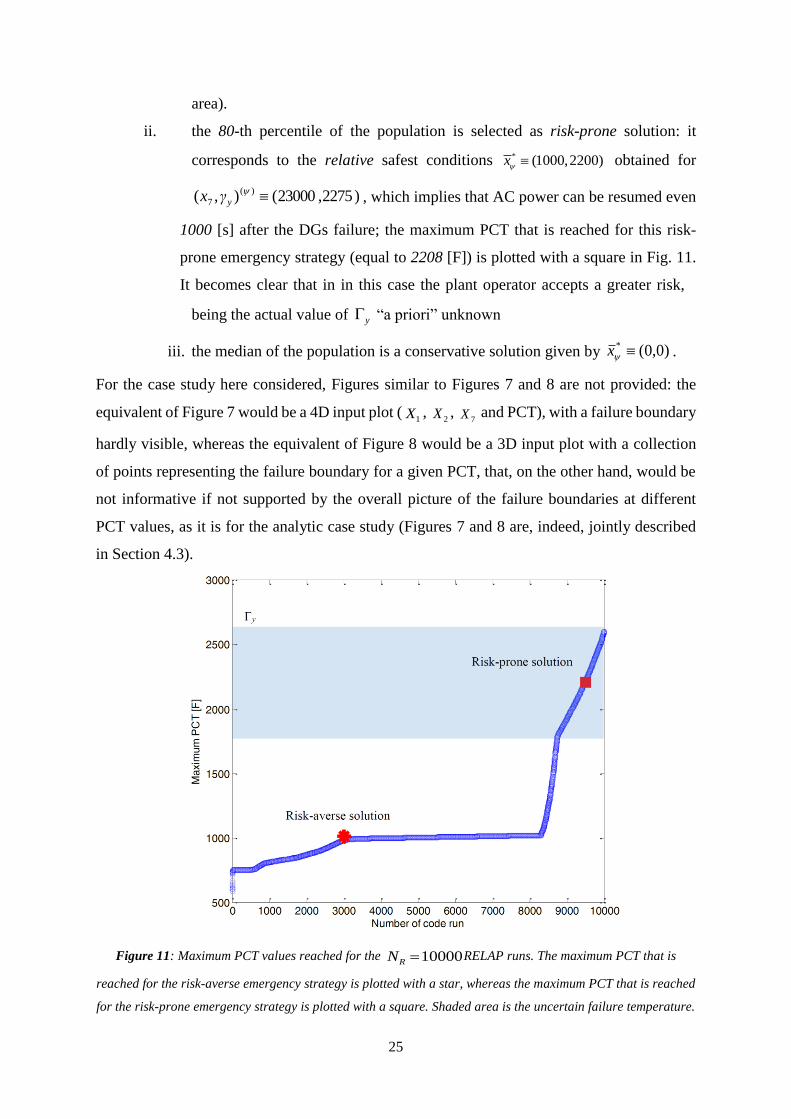
ii. the 80-th percentile of the population is selected as risk-prone solution: it
corresponds to the relative safest conditions * (1000,2200)x obtained for
)2275,23000(),( )(
7
yγx , which implies that AC power can be resumed even
1000 [s] after the DGs failure; the maximum PCT that is reached for this risk-
prone emergency strategy (equal to 2208 [F]) is plotted with a square in Fig. 11.
It becomes clear that in in this case the plant operator accepts a greater risk,
being the actual value of y “a priori” unknown
iii. the median of the population is a conservative solution given by )0,0(* x .
For the case study here considered, Figures similar to Figures 7 and 8 are not provided: the
equivalent of Figure 7 would be a 4D input plot (1X ,
2X , 7X and PCT), with a failure boundary
hardly visible, whereas the equivalent of Figure 8 would be a 3D input plot with a collection
of points representing the failure boundary for a given PCT, that, on the other hand, would be
not informative if not supported by the overall picture of the failure boundaries at different
PCT values, as it is for the analytic case study (Figures 7 and 8 are, indeed, jointly described
in Section 4.3).
Figure 11: Maximum PCT values reached for the 10000RN RELAP runs. The maximum PCT that is
reached for the risk-averse emergency strategy is plotted with a star, whereas the maximum PCT that is reached
for the risk-prone emergency strategy is plotted with a square. Shaded area is the uncertain failure temperature.
26
One can also consider that the estimated failure domain F~
might not be a compact space and,
then, larger percentile values of the *
x population might not necessarily correspond to larger
values of *
1x and *
2x , as in this particular case.
As a final remark on the case study considered in this Section, it is noted that a possible
demonstration of the efficiency of the adaptive sampling algorithm could be sought by the
following methodology:
1) Initialize the training with 50-100 RELAP5 simulations through LHS, grid or stratified
sampling (any space-filling experimental design). A total of 50-100 SBO simulations using a
system TH code is a practical limit for the number of simulations that can be performed on any
modern desktop computer in about one day and for the output to be easily verified by the
analyst.
2) Implement the adaptive sampling strategy using batches of 25-50 simulations per batch. The
existing 10000 data set is a good benchmark resource to compare with the evolving limit
surface.
3) Both the persistence requirement Eq. (6) and an engineering judgment should be used to
determine when the algorithm is to be stopped. If the P-ROM or B-ROM is suffering from
overfitting, the limit surface may be identified but the algorithm will not converge.
6. CONCLUSIONS
The RISMC program, sustained by the U.S. DOE, is engaged in the development of new
methods and tools to support effective decision making on NPPs life extension and licensing
of new nuclear technologies.
The present paper represents a contribution to this vast and ambitious program, as it sets forth
an adaptive sampling algorithm that embeds a support vector machine (SVM) for multivariate
regression, a SVM for classification, and a K-D tree search algorithm for nearest neighbor
search in multi-dimensional space to identify the NPP safest operating conditions in the
subspace of controllable variables as a function of distance from a limit surface under aleatory
and epistemic uncertainties. The partitioning of the model inputs into two subspaces of
controllable and non-controllable variables allows, indeed, the non-controllable variables to be
treated probabilistically and the safest operating conditions to be defined as a function of risk,
being the ultimate goal of the analysis to guarantee the required plant safety margins in accident

27
scenarios. We demonstrate that multivariate parameter sampling, surrogate/reduced
order/regression models, classification models and limit surface can yield practical, useful
results for the NPPs safety assessment.
The proposed approach has been applied to two case studies, i.e., a proof of concept using an
analytical example and a Loss of Offsite Power (LOOP) followed by a Station Black Out (SBO)
accident occurring in a Boiling Water Reactor with Mark I containment. In particular, the SBO
study involved a 3D SVM for regression, a 4D SVM for classification, and a 4D/2D K-D tree.
Coherently with the RISMC main objective, as a result of the application of this suite of
algorithms, various options are presented to the analyst to set the NPP in the safest operating
conditions: risk-averse, risk-prone decisions have been defined and illustrated, together with a
strategy that strikes a balance between these two extremes by identifying the plant “mean”
safest operating conditions. Even if practically viable for this case, the extension of the
presented approach to higher-dimensional problems should be further investigated from the
computational point of view, the K-D tree suffering a curse of dimensionality when dealing
with D larger than 20. In any case, as here proposed, a prior sensitivity analysis aimed at
reducing the multi-dimensional controllable variable space would tackle the computational
problem without the need to resort to other searching algorithms.
ACKNOWLEDGEMENT
The authors would like to thank all the reviewers for their valuable comments to improve the
quality of this paper.

28
APPENDIX
SVMs are a set of supervised learning methods that can be used for: i) classification, ii)
regression, iii) outliers or novelty detection [Basudhar et al., 2008; Cortes et al., 1995; Guyon
et al., 1993].
When a set of N training points ( N0 ) in a multi-dimensional space is given and
each point is associated with one of two classes characterized by a value 1z , the SVM
algorithm finds the boundary (i.e., decision function) that optimally separates the training data
into the two classes [Basudhar et al., 2008].
In the case of linear decision functions (i.e., the training data is linearly separable), the idea is
to maximize the margin between two parallel hyper-planes that separate the training data. The
pair of hyper-planes is required to pass at least through one of the training points of each
class (i.e., support vectors) and no points are admitted inside the margin. The optimization
problem whose solution determines the optimal pair of hyper-planes is [Basudhar et al., 2008]:
2
, 2
1min w
bw
(1A)
subject to 01)( bwz , N0
where w is the vector of the hyper-plane coefficients, b the bias and 2
2
w the distance
between the two hyper-planes. Problem (1A) is a Quadratic Programming (QP) problem that
can be solved through the method of Lagrange multipliers .
For the case of non-linear decision functions, non-negative slack variables are introduced
[Basudhar et al., 2008; Cortes et al., 1995]:
N
bwCw
1
2
,, 2
1min (2A)
subject to 1)( bwz , N0

29
The original set of variables can be mapped to a higher dimensional space, where the
classification of any test point is obtained by the sign of function:
),(1
e
N
Kzbs
(3A)
Where ),( eK is a kernel function. Common types of kernel functions used with SVM are:
Gaussian, polynomial kernels, multilayer perceptrons, Fourier series and splines [Basudhar et
al., 2008; Guyon et al., 1993].
30
REFERENCES
[Alvarenga et al., 2015] M. A. B. Alvarenga and P. F. Frutuoso e Melo. Including
Severe Accidents in the Design Basis of Nuclear Power Plants: an Organizational Factors
Perspective after the Fukushima Accident. In Annals of Nuclear Energy, Vol. 79, pp. 68-77.
Elsevier, May 2015.
[Apostolakis, 1990] G. E. Apostolakis. The Concept of Probability in Safety
Assessments of Technological Systems. In Science, Vol. 250, pp. 1359-1364. December 1990.
[Banks et al., 2011] H. T. Banks and H. Shuhua. Propagation of Uncertainty in
Dynamical System. In Proceedings 43rd ISCIE International Symposium on Stochastic Systems
Theory and Its Applications. October 2011.
[Basudhar et al., 2008] A. Basudhar, S. Missoum and A. H. Sanchez. Limit State
Function Identification Using Support Vector Machines for Discontinuous Responses and
Disjoint Failure Domains. In Probabilistic Engineering Mechanics, Vol. 23, pp. 1-11. Elsevier,
2008.
[Bentley, 1975] J. L. Bentley. Multidimensional Binary Search Trees Used for
Associative Searching. In Communications of the Association for Computing Machinery, Vol.
18, pp. 509-517. September, 1975.
[Bourinet et al., 2011] J. M. Bourinet, F. Deheeger and M. Lemaire. Assessing Small
Failure Probabilities by Combined Subset Simulation and Support Vector Machines. In
Structural Safety, Vol. 33, pp. 343-353. Elsevier, September 2011.
[Cadini et al., 2014] F. Cadini, F. Santos and E. Zio. An Improved Adaptive Kriging-
Based Importance Technique for Sampling Multiple Failure Regions of Low Probability. In
Reliability Engineering & System Safety, Vol. 131, pp. 109-117. Elsevier, November 2014.
[Chakraborty et al., 2015] S. Chakraborty and R. Chowdhury. A Semi-Analytical
Framework for Structural Reliability Analysis. In Computer Methods in Applied Mechanics

31
and Engineering, Vol. 289, pp. 475-497. Elsevier, February 2015.
[Cortes et al., 1995] C. Cortes and V. Vapnik. Support Vector Networks. In Machine
Learning, Vol. 20, pp. 273-297. Kluwer Academic Publishers, 1995.
[DOE, 2009] VV. AA. Light Water Reactor Sustainability Research and Development
Program Plan. Fiscal Year 2009-2013. DOE Office of Nuclear Energy, 2009.
[Gavrilas et al., 2004] M. Gavrilas, J. Meyer, B. Youngblood, D. Prelewicz and R.
Beaton. A Generalized Framework for Assessment of Safety Margins in Nuclear Power Plants.
In Proceedings to BE 2004: International Meeting on Updates in Best Estimate Methods in
Nuclear Installations Safety Analysis, pp. 28-36. November, 2004.
[Guyon et al., 1993] I. Guyon, B. Boser and V. Vapnik. Automatic Capacity Tuning of
Very Large VC-Dimension Classifier. In Advances in Neural Information Processing, pp. 147-
155. Morgan Kaufmann, 1993.
[Helton et al., 2011] J. C. Helton and J. D. Johnson. Quantification of Margins and
Uncertainties: Alternative Representations of Epistemic Uncertainty. In Reliability
Engineering & System Safety, Vol. 96, pp. 1034-1052. Elsevier, September 2011.
[Katayama et al., 2000] N. Katayama and S. Satoh. Experimental Evaluation of Disk-
Based Data Structures for Nearest Neighbor Searching. In DIMACS: Series in Discrete
Mathematics and Theoretical Computer Science, Vol. 59, pp. 87-104. American Mathematical
Society, 2000.
[Lucia et al., 2004] D. J. Lucia, P. S. Beran and W. A. Silva. Reduced-Order Modeling:
New Approaches for Computational Physics. In Progress in Aerospace Sciences, Vol. 40, pp.
51-117. Elsevier, February 2004.
[Mandelli et al., 2013] D. Mandelli, C. Smith, T. Riley, J. Schroeder, C. Rabiti, A.
Alfonsi, J. Nielsen, D. Maljovec, B. Wang and V. Pascucci. Support and Modeling for the
Boiling Water Reactor Station Black Out Case Study using RELAP and RAVEN. Idaho
National Laboratory Technical Report. 2013.

32
[Mandelli, 2014] D. Mandelli. Simulation of a SBO accident for the BWR Mark I
Nuclear Power Plant Model by the RELAP5-3D Code. Private Communication, 2014.
[Maneewongvatana et al., 2001] S. Maneewongvatana and D. M. Mount. On the
Efficiency of Nearest Neighbor Searching with Data Clustered in Lower Dimensions. In
Proceedings of the International Conference on Computational Sciences, pp. 842-851.
Springer-Verlag, 2001.
[Mohsine et al., 2010] A. Mohsine and A. El Hami. A Robust Study of Reliability-
Based Optimization Methods under Eigen-Frequency. In Computer Methods in Applied
Mechanics and Engineering, Vol. 199, pp. 1006-1018. Elsevier, 2010.
[Möller et al., 2008] B. Möller and M. Beer. Engineering Computation under
Uncertainty –Capabilities of Non-Traditional Models. In Computer & Structures, Vol. 86, pp.
1024-1041. Elsevier, May 2008.
[Rabiti et al., 2014a] C. Rabiti, A. Alfonsi, J. Cogliati, D. Mandelli and R. Kinoshita.
Introduction of Supervised Learning Capabilities of the RAVEN Code for Limit Surface
Analysis. In Transactions of the American Nuclear Society, Vol. 110, pp. 355-358. June, 2014.
[Rabiti et al., 2014b] C. Rabiti, A. Alfonsi, J. Cogliati, D. Mandelli and R. Kinoshita.
RAVEN, a New Software for Dynamic Risk Analysis. In Probabilistic Safety Assessment and
Management Conference. June 2014.
[Schuëller et al., 2008] G. I. Schuëller and H. A. Jensen. Computational Methods in
Optimization Considering Uncertainties – An Overview. In Computer Methods in Applied
Mechanics and Engineering, Vol. 198, pp. 2-13. Elsevier, May 2008.
[Sherry et al., 2012] R. Sherry and J. Gabor. Pilot Application of Risk Informed Safety
Margins to Support Nuclear Plant Long Term Operation Decisions – Impacts on Safety
Margins of Power Uprates for Loss of Main Feed-Water Events. EPRI, December 2012.
[Stigler, 1989] S. M. Stigler. Francis Galton’s Account of the Invention of Correlation.

33
In Statistical Science, Vol. 4, pp. 73-79. 1989.
[Urbanic et al., 1981] V. F. Urbanic and T. R. Heidrick. High Temperature Oxidation
of Zircaloy-2 and Zircaloy-4 in Steam. In Journal of Nuclear Materials, Vol. 75, pp. 251.
Elsevier, August 1981.
[Xu et al., 2009] H. Xu, C. Caramanis, S. Mannor, Robustness and Regularization of
Support Vector Machines, Journal of Machine Learning Research, Vol. 10, 1485-1510, 2009.
[Zio et al., 2008] E. Zio and F. Di Maio. Bootstrap and Order Statistics for Quantifying
Thermal-Hydraulic Code Uncertainties in the Estimation Of Safety Margins. In Science and
Technology of Nuclear Installations, Vol. 2008, Article ID 340164. Hindawi Publishing
Corporation, 2008.
[Zio et al., 2010] E. Zio, F. Di Maio and J. Tong. Safety Margins Confidence Estimation
for a Passive Residual Heat Removal System. In Reliability Engineering & System Safety, Vol.
95, pp. 828-836. Elsevier, August 2010.
[Zio et al., 2012] E. Zio, F. Di Maio, Fatigue Crack Growth Estimation by Relevance
Vector Machines, Expert Systems with Applications, Volume 39, pp. Volume 39, Issue 12,
Pages 10681–10692, 2012.