An approach to surface retouching and mesh smoothing

Nikita Kojekine1, Vladimir Savchenko2, Michail Senin3, Ichiro Hagiwara4

1,4 Faculty of Engineering, Tokyo Institute of Technology, 2-12-1, O-okayama, Meguro-ku, Tokyo 152-8552, Japan. E-mail: karlson@stu.mech.titech.ac.jp, hagiwara@mech.titech.ac.jp 2 Faculty of Computer and Information Sciences, Hosei University, 3-7-2 Kajino-cho Koganei-shi, Tokyo 184-8584, Japan. E-mail: vsavchen@k.hosei.ac.jp 3 Moscow Institute of Physics and Technology, Kerchenskaya str., house 1"A", building 1, Moscow 113-303, Russia. E-mail: m_senin@mail.ru

In this paper, we discuss a novel fast practical algorithm for surface modification of geometric objects. A space-mapping technique is used to transform a given or damaged part of a surface into a different shape in a continuous manner. The proposed approach is used for the surface-retouching and mesh smoothing problems. The technique, in fact, is based on a local processing of polygonal data that can be applied for fairing of 3D meshes. We consider shape transformation as a general type of operation for surface modification, and attempt to approach the problem from a single point of view, namely that of the space-mapping technique based on implementation of radial bases functions. Experimental results are included to demonstrate the functionality of our mesh-modeling tool.

Key words: Radial basis functions, space mapping, surface retouching, mesh smoothing.

1 Introduction Many recent studies have focused on exploring shape transformation as a basic operation in computer graphics (CG) and computer-aided geometric design (CAGD). The operation involves transforming a given geometric shape into another in a continuous manner. Important examples of surface fitting and deformation have been intensively investigated in the past few years, and various strategies have been proposed to minimize the user interaction; however, the problem of fitting a surface to control points still remains a largely unsolved problem of great practical importance.

Point sets obtained from computer vision techniques are often non-uniform or even contain large areas of missing points. In some well-known algorithms, authors make the assumption that points are located sufficiently evenly. In others, it is assumed that holes have entirely specific shapes.

Another source of polygonal data with missing or damaged areas is partly destroyed ancient artifacts. In such applications, an incomplete surface is the surface exactly as measured, and the main problem is to obtain prospective reconstructions that look reasonable. For example, archeologists often acquire broken vessels, and 3D models of these artifacts are created by using laser digitizers on each piece. Complete reconstruction of broken objects is a difficult task. In this paper, we describe an approach to surface retouching of polygonally represented shapes that contain missing areas (holes) and damaged areas. Our software implementation of the proposed approach has two

options. As the first option, the user can manually define a region to be retouched. As the second option, the proposed solution begins by extracting the holes’ contour lines to define a region to be retouched, a rough stitching of the holes is applied next and then a linear subdivision of the retouched region is produced to generate a surface to be modified by subsequent space transformation operations.

The approach is based on the simple idea of shape transformation. Indeed, when we are using only generic properties such as position of a point of the object that is deformed, the problem of constructing a smooth surface satisfying certain constrains can be formulated as a space mapping from R3 to R3. We consider shape transformation as a general type of operation for restoring missing data, and attempt to approach the well-known problem of “fulfillment” of damaged or missing surface areas from a single point of view, namely, that of the space mapping technique. What is meant by shape transformation is a modification of points, predicted, for instance, by a linear subdivision of triangles resulting from a stitching of hole boundary points, as shown in Fig. 10 (second row).

Compactly supported radial-basis functions (CSRBFs), introduced by Wenland (Wendland 1995), is one of the most popular classes of radial-basis functions (RBFs) because they are strictly positive definite in R1,3,5. One of the most attractive features of RBFs is the simplicity of implementation, and researchers usually state that RBF methods guarantee automatic mesh repair and interpolation of large irregular holes. However, the work required for correct reconstruction of an object is nearly proportional to the total number of scattered data points. The amount of computation is thus significant, even for a moderate number of nodes. If we have a gap in our data set, we face the problem of evaluating the functions at extra point; if a radius of support is quite large in the assembly of a matrix of linear equations by CSRBF method, then the cycle associated with the matrix of linear equations will include nearly all the points of the input data. Moreover, reliable results in reconstruction cannot be achieved without a sufficiently uniform distribution of scattered data. To attain real-time processing of a huge amount of input data and avoid an over-smoothing inherent in isosurface extraction from an implicitly defined object, we replace the reconstruction process by the space-mapping technique. This allows disconnected surface areas to be reconstructed by using a sufficiently small radius of support, as we will demonstrate in various applications: surface recovering of missing 3D data and surface refinement.

The approach proposed here for surface retouching originates from the obvious relationship between 3D surface retouching (or reconstruction of missing data) and the 2D inpainting problem. For more references, see the pioneering work (Bertalmio et al. 2000), which describes an image-inpainting (non-texture) algorithm based on partial differential equations. See also the recent studies (Oliveira et al. 2001, Esedoglu and Shen, and Sarti et al. 2001). The main idea of the approach is to use the user-defined portions of the input image to be retouched (see Fig. 6 (b), red area). The algorithm treats the input image as three separate channels (R, G, and B), and fills in areas to be inpainted. Actually, image inpainting can be thought as an extrapolation problem in which information from outside a masked area propagates. It is known that the 3D space-mapping technique can be applied to surface modification. Naturally, user-selected data sets which are represented in the form z = f(x,y) after local transformation, where the z coordinate is used as one channel, can be used as control points. Thus the term “surface retouching” is used to denote the deformation of one

set of points into another between boundaries of boundary polygons, which define a hole or a retouching region.

Let us point out here that we clearly understand the limitations of the proposed technique. We have to notice that the results of surface retouching (see Fig. 9, 10) depend on points situated in a masked area and that the surface is a continuation of a region surrounding the region to be retouched. Nevertheless, according to our experiments (see Fig. 10, second row) stitching the nodes of damaged areas of 3D polygonal models by using triangles will produce clearly visible artifacts; and standard shape smoothing approaches are not appropriate for removing such shape defects, such as that shown in Fig. 8.

The principal contribution of this work is a novel surface-retouching algorithm based on a local approximation of missing data. We show that CSRBFs offer a mechanism for obtaining extrapolated points of a damaged surface; CSRBFs exhibit high-quality restoration results in surface-retouching examples, and that they are trivial to implement because of their simplicity. Since the proposed retouching technique, in fact, is based on a local processing of polygonal data, we also show the applicability of CSRBFs for fairing 3D meshes. We introduce a new mesh smoothing approach in terms of CSRBF interpolation. In the case of surface smoothing, a sequence of meshes generated by CSRBFs rapidly converges to a smooth surface. The proposed technique also illustrates their volume- and feature-preserving properties, in practice; after a smoothing step we do not scale a new volume back to its original volume. Our method is efficient, especially for large models, where existing methods are often not fast enough or exhibit excessive smoothing properties; we present an approach to obtain almost interactive response for sufficiently complex models (70K triangles) without off-line preprocessing. Moreover, our method can be applied to point sets. All the same, although we apply the approach based on the restoration of local “elevation data,” this technique is applied in 3D space and can also serve for sculpting (editing) a surface according to the user demands and for animation.

Some preliminarily results of this research were presented before in the paper (Kojekine and Savchenko 2002).

The rest of the paper is organized as follows. The next section gives a short overview of shape transformation techniques and studies related to the surface retouching problem. We discuss the notion of a 3D warping technique and software algorithm in Sec. 3. Application examples of surface recovering are presented in Sec. 4. Sec. 5 contains some conclusions.

2 Related works Mappings can be controlled by numerical parameters of predefined functions, by control points, and by differential equations. An overview of all transformation techniques is beyond the scope of this paper. We present here a short overview of papers concerning the problem.

Shape transformation is a useful tool for many applications such as computer animation, CAGD, forensic identification. Papers (Chen et al. 2000 and Skaria et al. 2001) present a very good overview of existing methods for shape reconstruction and modification. For more references, see (Wyvill and Van Overveld 1997).

A vast literature is devoted to the subject of scattered data interpolation, especially in the field of terrain reconstruction. In spite of a flurry of activity in the field of scattered data reconstruction and interpolation, this problem remains difficult

and computationally expensive. A very good overview of related studies, problems, and limitations can be found in the paper (Lee et al. 1997), which addresses these problems and introduces a very fast algorithm for constructing C2-continuous parametric interpolation functions. The algorithm applies an effective B-spline technique based on the multilevel B-spline approximation (see Lee at al. 1995).

Using piecewise polynomial functions sometimes leads to undesirable excessive smoothing of the reconstructed surface. This problem is far from the solution because, as mentioned in the paper (Gousie and Franklin 1998), the desirable characteristics of an interpolation or approximation algorithm are not obvious, since different attributes conflict with each other. Schneider (Schneider 1998) states that clearly visible artifacts affect almost all recent terrain models. Applying higher degree interpolants is rather popular, nevertheless let us cite here the opinion expressed in (Gousie and Franklin 1998): “second-degree continuity might be a desirable attribute, except that the real world is often not continuous at all.”

Shape reconstruction from given points can be thought of as a special case of transformation. One approach is to use methods of scattered data interpolation based on the minimum-energy properties (Ahlberg et al. 1967, Dushon 1976, Vasilenko 1983). These methods are widely discussed in the literature (see also Bolle and Vemuri 1991 and Greiner 1994).

The benefits of modeling with the help of RBFs have been recognized in many studies. To the best of our knowledge, the first publications on using discrete 2D landmark points were those of Bookstein (Bookstein 1989, Bookstein 1991). RBFs were adapted for computer animation (Litwinovicz and Williams 1994), medical applications (Carr at al. 1997, Bookstein 1989), and for surface reconstruction (Savchenko et al. 1995, Turk and O’Brien 1999). However, the required computational work is proportional to the number of grid nodes and the number of scattered data points. Special methods for reducing the processing time were developed for thin plate splines, and were discussed in (Beatson and Light 1994, Light 1994, and Carr et al. 2001).

In spite of significant progress in the field of implementing RBFs and CSRBFs (Morse et al. 2001, Kojekine et al. 2003) for reconstruction purposes, it is still an open question whether it is possible to handle realistic amounts of data in real time. We suppose that they are suitable for sufficiently moderate 3D data sets; for instance, execution time is about 300 seconds for 36000 points, without time expenses for surface extraction, as was reported in (Morse et al. 2001).

Methods of reconstruction of a model based on global reconstruction by using RBFs and CSRBFs produce sufficiently good approximation of a surface, nevertheless they suffer from two drawbacks. They do cost a great deal of time and artifacts or “ghost” objects appear as a result of extraction of a geometric shape from an implicitly defined function, see recent work (Ohtake et al. 2003). Nevertheless, RBFs possess many features that make them very attractive for CAGD applications dealing with modification of geometric objects.

Problems involved in reconstructing missing portions of geometric objects that appear in CAGD have been investigated in the past few years. Three approaches have been dominant in the CAGD area: the first one works with 3D polygonal models to stitch damaged or incorrectly calculated nodes of 3D geometric objects (Barequet and Sharir 1993), the second one is an approach that deals with fitting the generated data according to some geometrical features such as curvature (for more references, see Hermann et al. 1997), and the third one is

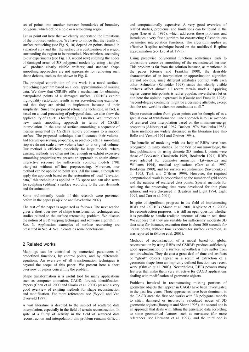
actually based on a mathematically well-founded set-level approach. Partial differential equations are widely used to model a surface subject to certain constraints (see Bloor and Wilson 1996 and Setian 1996). The paper (Whitaker and Breen 1998) gives an exhaustive overview of this topic; their paper presents an improved numerical algorithm that solves particular problems in geometric modeling. Nevertheless, RBFs, PDE, FEM methods demonstrate undesirable terracing and ringing effects, as discussed in (Gousie and Franklin 1998). Fig. 1 shows an example of FEM reconstruction of Mount Bandai discussed in (Savchenko and Sedukhin 2001).

(a) (b) (c) Fig. 1. (a) A vertical crosscut of the fragment of Mount Bandai. (b) FEM approximation of a surface from a limited number of contour maps with a smoothing parameter α = 0.1. (c) Approximation of a surface with α = 2.8.

A different way of reconstructing missing portions of geometric objects is to use a “cloning” approach, see, for instance the work (Savchenko and Schmitt 2001) where an application of a 3D-space-mapping technique and numerical optimization with a specially designed genetic algorithm to a problem concerning CAGD in dentistry was presented. But this approach has two main drawbacks. In the first place, a standard or “cloning” surface should be given. Second, human knowledge and experience is necessary to assign initial correspondence points to compensate for the gap between the region of restoration and the existing part of the object.

Another approach to surface retouching based on using a bending energy was proposed in (Savchenko and Kojekine 2002). But the main drawback of this algorithm is that an optimization technique should be used to avoid superfluous folding over the reconstructed region.

(Davis et al. 2002) presented a new technique for applying a diffusion process to extend a signed distance function through the volume for surfaces containing geometrically and topologically complex holes, which arise in practice when range measurement systems provide point sets that may be incomplete. The method is simple and effective; nevertheless, one of the main problems, according to the authors, is the sensitivity of the functions to the distance at which they clamp these functions. Unfortunately, time performance of the algorithm is not discussed.

The points obtained often exhibit rough features due the inevitable physics noise added by a scanning device. Many methods for curve and surface interrogation and smoothing have been discussed in context of differentional geometry (see Farin 1998 and references therein). A vast mathematical literature is devoted to the subject of construction of smoothing splines (see, for instance, (Craven and Wahba 1979)), where a practical, effective method for estimating the optimum amount of smoothing from the data is presented.

In recent years, the CG community has paid more attention to mesh smoothing based on a signal processing approach, pioneered by Taubin in 1995 (Taubin 1995). A Laplacian smoothing is considered in (Desbrun et al. 1999) where time integration of the heat equation on an irregular mesh and a curvature flow approach is used to remove undesirable noise.

The algorithm of Desbrun et al. is very fast, however an over smoothing can be observed in Figure 5 of their paper.

Subdivision schemes (Warren and Weimer 2002) can be thought of as an alternative approach to the problem. Nevertheless, subdivision schemes are able to deal with arbitrary topology but not with arbitrary connectivity, as was mentioned in (Kobbelt et al. 1998).

A fast mesh-smoothing algorithm based on the multi-resolution technique in combination with the constrained minimization of discrete energy functional has been proposed (see (Kobbelt et al. 1998)). Using mesh hierarchies, where components of the geometric shape are characterized by fairing on each level of details, solves the problem. It leads to interactive response times for moderately complex models, with about 5K triangles. Nevertheless, off-line preprocessing (an incremental mesh decimation algorithm) must be applied.

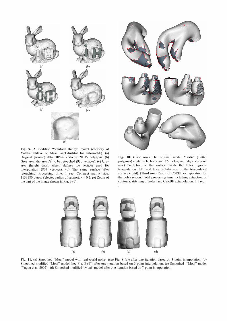
Many authors have very carefully considered the questions of geometric distortion during smoothing and problems of precise shaping (see, for instance, the recent papers Zhang and Fiume 2002 and Yagou et al. 2002, where algorithms to preserve the sharp features of a mesh were presented, see also Yagou et al. 2003). They provide excellent feature-preserving behavior. However, a number of issues in their application remain open problems in need of a more thorough examination. For example, while preserving features they can produce additional artifacts, as it shown in Fig. 11(c).

3 The Algorithm For an arbitrary n dimensional area Ω that contains a set of points Pi = (x1

i, x2i, …, xn

i) : i = 1, 2, … , N , volume splines interpolating scattered data can be used as a solution for creating mapping functions. The interpolation is the variational solution that defines a linear operator T under the following minimum condition:

∫ ∑Ω =m||α

m!/α!(Dαf)2dΩ → min,

where m ≥ 2 is a parameter of the variational functional and α is a multi-index. This spline is based on the Green’s function and in the 2D case it is the so-called thin spline (see Dushon 1976, Vasilenko 1983). It is equivalent to using the radial basis functions φ(r) = r2m-nln(r) and r2m-n for n = 2 and 3, respectively, where r is the Euclidean distance between two points. Since the function φ(r) is not compactly supported, the corresponding system of linear algebraic equations (SLAE) is not sparse or bounded. Storing the lower triangle matrix requires O(N2) real numbers, and the computational complexity of a matrix factorization is O(N3). Thus, the amount of computation becomes significant, even for a moderate number of points.

Wendland (Wendland 1995) constructed a new class of positive definite and compactly supported radial functions for 1D, 3D and 5D spaces of the form

φ(r) = ( )

>≤≤

1r01r0r

,,ψ ,

where ( )rψ is a univariate polynomial whose radius of support is equal to 1. Scaling of the function )( αψ /r allows any desired radius of support α . In our application we have selected a simple function:

( ) ( )r1 2r −

+=ψ In practice, the reconstruction operation consists of the

following steps: data sorting for the landmark area ΩL, construction of an SLAE, solution of the SLAE, and evaluation of the mapping functions for a region to be retouched. In fact, while the solution of the system is the limiting step, construction of the matrix and evaluation of the functions may also be computationally expensive.

which is an interpolated function that supports only C0 continuity. However, other functions that support a higher continuity can be applied. An investigation (Wendland 1999) of the smoothness of this family of polynomial basis functions shows that each member φ(r) possesses an even number of continuous derivatives. Our first goal is to build an octal tree data structure from the

original point data. Afterwards this tree is used to search for neighbors of any point among the given N points. The neighbors are points of a sphere of radius r whose origin is located at the given point.

The volume spline f(P) having values hi at N points Pi is the function

f(P) = γ∑=

N

j 1jφ (|P - Pj|) + p(P), ♦

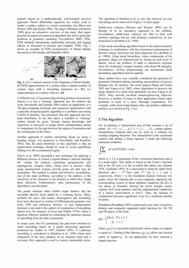
To make the sub-matrix A band-diagonal, we need to renumber the initial points in a special way. An efficient approach based on the use of variable-depth octal trees for space subdivision has been proposed (Kojekine et al. 2003). It allows us to obtain the resulting matrix as a band-diagonal matrix that reduces the computational complexity. As a result of applying this algorithm, a band-diagonal sub-matrix is constructed as shown in Fig. 2.

where` p = ν0 + ν1x + ν2y + ν3z is a one degree polynomial. To solve for the weights γj we have to satisfy the constraints hi by substituting the right part of the equation ♦, which gives

hi = γ∑=

N

j 1jφ(|Pi - Pj|) + p(Pi),

To store the band-diagonal matrix A, we use a so-called profile form or a slightly modified Jennings envelope scheme (Jennings 1996). An array can be used for diagonal elements; values of non-diagonal elements and corresponding indices of the first non-zero elements in the matrix lines are placed in two additional arrays.

Solving for the weights γj and ν0,ν1,ν2,ν3 it follows that in the most common case there is a doubly bordered matrix T, which consist of three blocks, square sub-matrices A and D (matrix with zero elements, which defines a kernel of the operator T) of the size N× N and 4 × 4 (for n = 3) respectively, and B, which is not necessarily square and has the size N × 4.

In practice, the technique requires that a masked surface represented by polyhedrons be a closed, oriented manifold embedded in 3-D space and have the property that, around every one of its points, there exists a neighborhood that is homeomorphic to a disc. That is, we can deform the surface locally into the plane without tearing it or identifying separate points with each other. We employed an approach that uses displacements of N control points as a difference between an initial and final geometric form. The approach provides local deformations of data points homeomorphic to a disc; nevertheless, it is important to reiterate here that we formulate the surface-retouching problem in terms of the space-mapping technique, where transformations in x,y,z directions are allowed. Interpolation of (x,y,z) points is implemented in R3 and defines a relationship between coordinates of points in the original and deformed objects. Landmarks situated in the mask area Ω+ defined by the user (Fig. 7 (b), red square) naturally do not belong to the area ΩR to be retouched (Fig. 7 (a)). The difference between Ω+ and ΩR defines the landmark area ΩL. The inverse mapping function that interpolates the z-heights and is needed to calculate reconstructed (destination) points z d

is given in the form

Fig. 2. Example of a sub-matrix A (580x580) for the example shown in Fig. 6(a).

For a symmetric and positive definite matrix, a special factorization, called Cholesky decomposition, is about twice as fast as alternative methods for solving linear equations by Gaussian LU decomposition (see Press at al. 1997). A combination of block Gauss solution and Cholesky decomposition was proposed (George and Liu 1981), and in our software tools we follow their proposal. Naturally, implicit or conjugate gradient methods can be used. Because such methods use the maximum number of allowed iterations and the desirable convergence tolerance we prefer to use explicit methods for the SLAE solution.

The algorithm for surface smoothing actually relies upon the premise that around each surface point, there exists a neighborhood that is homeomorphic to a disc. To satisfy this condition, we process points nearest to the point, which should be moved according the calculated differences or deviations for local z-directions that define the inverse mapping function. The user can define a local z-direction in a simplest case by an appropriate rotation of the whole geometric object.

zs = f(P) + zd,

where the components of the volume splines f(P) interpolating displacements of starting points zs are used to calculate points that belong to the area ΩR. The surface-retouching problem is formulated in terms of the space-mapping technique for 3D space. Z-directional transformations will obviously cause a translation of a geometric model in some direction. To avoid such a translation, we assign 8 boundary constraints − (x,y,z) coordinates of unit cube bounding a retouched region. By this means the matrix size is N = 8 + NL+ + 4, where NL+ is the number of points belonging the landmark area. A right part of the SLAE consists of the 8 zero values, NL+ values of differences between zs

i and zdi (i = 1,2, …, NL+), and 4 zero

values corresponding to the matrix D.

However, for some holes, where a surface variation is large, if for instance, variation σ is larger then 0.3 − that is, if the data demonstrate a strong deviation from an average plane − this simple algorithm cannot be applied (see for example the hole in the branching area in Fig. 10). In this case, we apply a local retouching strategy, i.e. we require that a reconstructed point of a surface should have the property that, around the point, there exists a neighborhood that is homeomorphic to a disc. To satisfy this condition we proceed as follows:

• build an octal tree based on all original points of the model;

• extract all non-intersecting border polygonal lines or the borders of holes (an algorithm of finding non-intersecting border polygonal lines is omitted because of constrains on space)

• apply a point stitching method (description is omitted , some comments are given below)

• obtain new points inside the hole region after stitching of vertices by using linear subdivision;

• for each new point (x,y,z) inside the hole region: • define the nearest plane for neighborhood points from

the octal tree for the point (x,y,z), rotate these points so that the nearest plane is perpendicular to the z-axis, and project the original neighborhood points to the OXY plane;

• calculate z-deviations and define CSRBF mapping functions;

• apply this transformation to the projection of the point (x,y,z);

• produce the inverse rotation of this transformed point and add the result to the octal tree.

Naive triangulation of holes with non-disc topology often yields self-intersections; other holes have multiple self-intersecting points that have to be distinguished. Thus on the first step of our algorithm we solve the hole extraction problem. Then we apply a rough stitching of the hole boundary vertices. Application of dynamic programming makes it possible to avoid multiple repetitions of a consideration of the same sets of faces for different triangulations of a polyhedron region as has been described in the book (Cormen at al. 1992). Also, in spite of the fact that features of the reconstructed surface are unknown, it is desirable to get the “smoothest” triangulation, which is useful for the subsequent step of surface improvement. In our application we use recurrent correlations, which offer the possibility of finding well-defined triangulations, but it is more useful to find the smoothest one for obtaining an optimal triangulation of the holes’ boundary polygonal lines, see Fig. 10, second row, left image. We are therefore looking for a triangulation where we can minimize the sum of scalar multiplications of normal vectors ni

r of the face i and normal

vectors , and n of neighboring faces. 21, ii nn rr3ir

Once we have extracted information about the borders of the holes, we need to estimate local surface properties, which can be done by estimating the tangent plane. Hoppe et all. (Hoppe et al. 1992) have demonstrated that eigenvalues λ1, λ2, λ3 of the covariance matrix of neighborhood points can be used to produce normal estimation. The values λ1, λ2, λ3 describe the surface variation σ and can serve as an analog of a surface curvature that is used in our software implementation to make a decision about the complexity of the retouching region. Assuming that λ1 is minimal, λ1 describes the variation along the surface normal, and directions corresponding to the eigenvalues λ2, λ3 define a tangent plane.

If for the hole border a surface variation σ is sufficiently small, then a simple projection of the hole border on the plane will also give a non-intersecting polygonal line. In this simple case, we can easily find (by using an octal tree) the landmark area ΩL (see, for example, the gray area in Fig. 9 (c)).

Our smoothing algorithm is almost similar to the technique discussed above. The algorithm is sufficiently simple and is based on an iterative procedure to perform smoothing

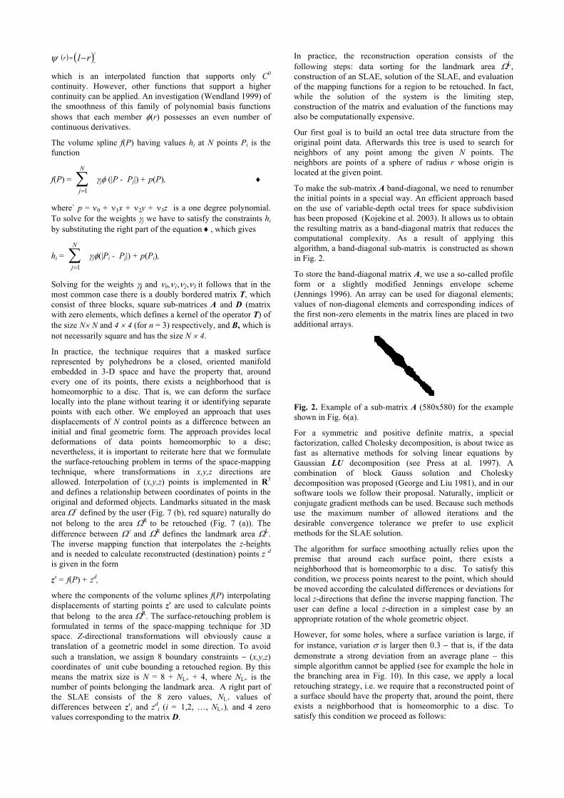
operations. In each iteration step, a point belonging to a shaped polygon (number of points can be defined by the user or according to a radius of support, which defines in this a case a masked area) is processed in accordance with the inverse mapping function. We rotate the mask area points so that the tangent plane for the masked area is perpendicular to the z-axis. Then we calculate a CSRBF shape transformation from projected to original points and apply it to the processed point. Such a technique is applied for rotating an oriented pyramid (defined by the union of faces adjacent to the processed vertex, as shown in Fig. 3) centered at a processed point and for its neighborhood points.

Fig 3. Illustration of an oriented pyramid.

Let us note that the surface variation σ can be used as an estimation of a local curvature of current mesh to distinguish the areas having different geometric characteristics for preserving object features.

4 Experiments Notice that in all the examples (except Fig. 7) in this paper the processing time is shown for our test configuration AMD Athlon 1000 Mhz, 128 MB RAM, Microsoft® Windows 2000.

4.1 Surface smoothing

Fig. 4 shows a comparison between the proposed CSRBF smoothing technique and Laplacian smoothing method. Fig. 5 and 11 show the effect of CSRBF smoothing on polygonal surfaces and Table 1 shows the processing time benchmarks and errors (the difference from the original model). To define the inverse mapping function, a different number of vertices N can be used for interpolation. The larger the number N we select, the more feature-preserving smoothing will be performed (compare the images in Fig. 5 (b) and (c)) and the more accurately the volume will be preserved (see Table 1). To achieve higher smoothing effect several iterations of the above algorithm could be applied (see Fig. 5 (d)).

4.2 Surface retouching

Floating point arithmetic is used; thus, before processing the input data we prefer to normalize them in order to reduce the number of possible truncation errors. To illustrate the applicability of the space-mapping technique to the surface-retouching problem, we first show in Fig 6 examples of image inpainting. Fig. 6(a), (left image) is a damaged picture of a dragonfly; Fig. 6 (a) (right image) is a result of restoration based on a global reconstruction. Image size: 550 × 388 24bpp. Size of ΩR area: 380 pixels. Size of ΩL area: 580 pixels. Data sorting: 0.02 sec. LLt decomposition, forward and back substitution: 0.02 sec. Reconstruction time: 0.02 sec.

Fig. 6 (b) shows that using locally defined neighboring points from a landmark area ΩL initially surrounding the scratch produces sufficiently good visual appearance of the retouched scratch for a textured image. In this example a simple strategy

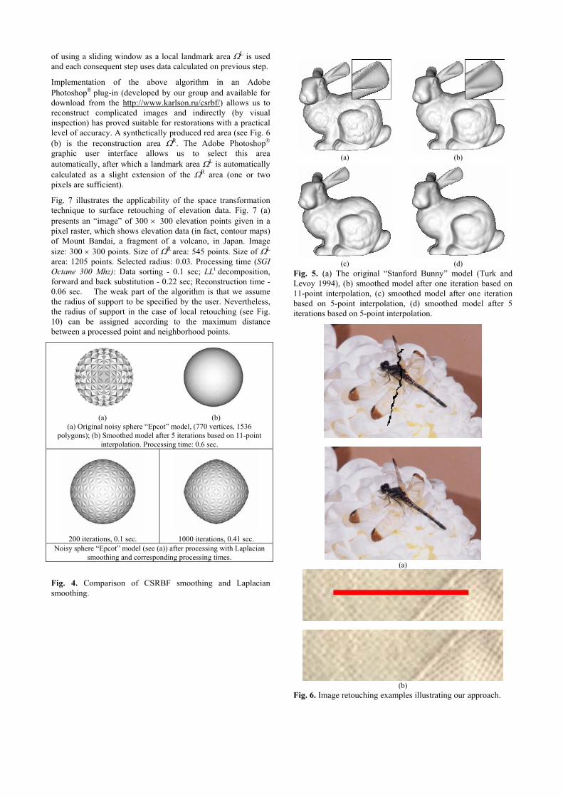
of using a sliding window as a local landmark area ΩL is used and each consequent step uses data calculated on previous step.

(a)

(b)

(c)

(d)

Implementation of the above algorithm in an Adobe Photoshop plug-in (developed by our group and available for download from the http://www.karlson.ru/csrbf/) allows us to reconstruct complicated images and indirectly (by visual inspection) has proved suitable for restorations with a practical level of accuracy. A synthetically produced red area (see Fig. 6 (b) is the reconstruction area ΩR. The Adobe Photoshop graphic user interface allows us to select this area automatically, after which a landmark area ΩL is automatically calculated as a slight extension of the ΩR area (one or two pixels are sufficient).

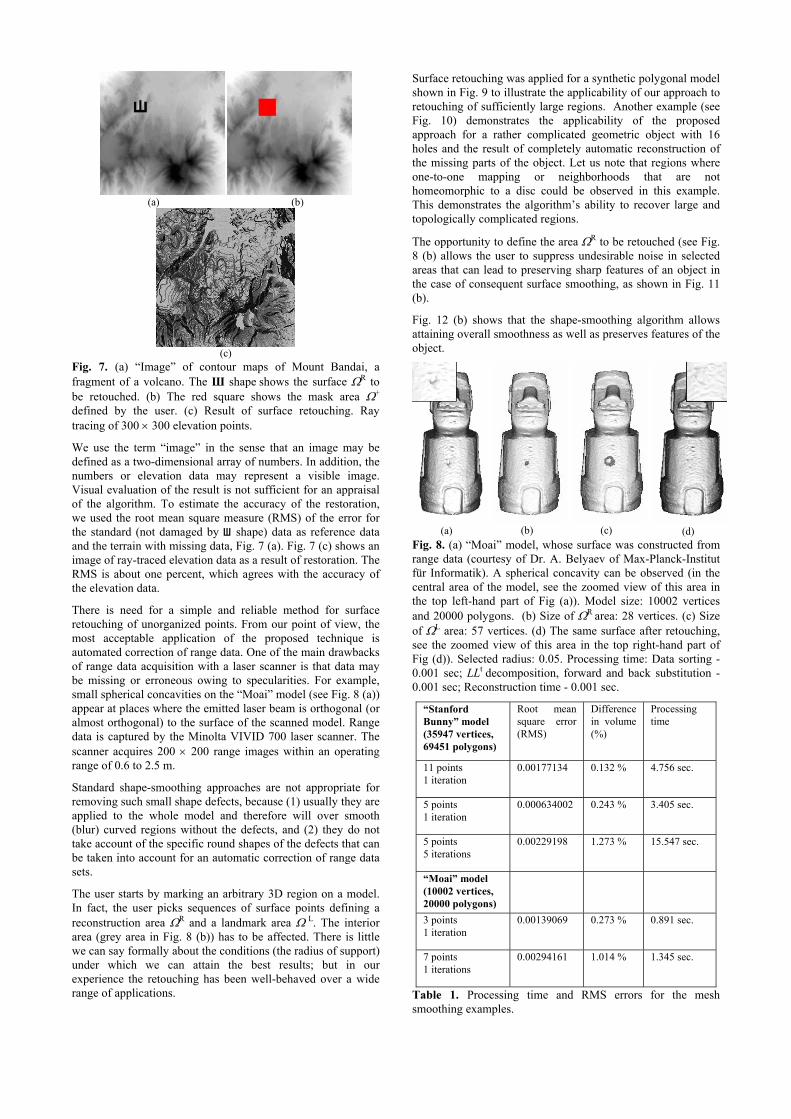
Fig. 7 illustrates the applicability of the space transformation technique to surface retouching of elevation data. Fig. 7 (a) presents an “image” of 300 × 300 elevation points given in a pixel raster, which shows elevation data (in fact, contour maps) of Mount Bandai, a fragment of a volcano, in Japan. Image size: 300 × 300 points. Size of ΩR area: 545 points. Size of ΩL area: 1205 points. Selected radius: 0.03. Processing time (SGI Octane 300 Mhz): Data sorting - 0.1 sec; LLt decomposition, forward and back substitution - 0.22 sec; Reconstruction time - 0.06 sec. The weak part of the algorithm is that we assume the radius of support to be specified by the user. Nevertheless, the radius of support in the case of local retouching (see Fig. 10) can be assigned according to the maximum distance between a processed point and neighborhood points.

Fig. 5. (a) The original “Stanford Bunny” model (Turk and Levoy 1994), (b) smoothed model after one iteration based on 11-point interpolation, (c) smoothed model after one iteration based on 5-point interpolation, (d) smoothed model after 5 iterations based on 5-point interpolation.

(a) (b)

(a) Original noisy sphere “Epcot” model, (770 vertices, 1536 polygons); (b) Smoothed model after 5 iterations based on 11-point

interpolation. Processing time: 0.6 sec.

200 iterations, 0.1 sec.

1000 iterations, 0.41 sec.

Noisy sphere “Epcot” model (see (a)) after processing with Laplacian smoothing and corresponding processing times.

(a)

(b)

Fig. 4. Comparison of CSRBF smoothing and Laplacian smoothing.

Fig. 6. Image retouching examples illustrating our approach.

Surface retouching was applied for a synthetic polygonal model shown in Fig. 9 to illustrate the applicability of our approach to retouching of sufficiently large regions. Another example (see Fig. 10) demonstrates the applicability of the proposed approach for a rather complicated geometric object with 16 holes and the result of completely automatic reconstruction of the missing parts of the object. Let us note that regions where one-to-one mapping or neighborhoods that are not homeomorphic to a disc could be observed in this example. This demonstrates the algorithm’s ability to recover large and topologically complicated regions.

(a) (b)

The opportunity to define the area ΩR to be retouched (see Fig. 8 (b) allows the user to suppress undesirable noise in selected areas that can lead to preserving sharp features of an object in the case of consequent surface smoothing, as shown in Fig. 11 (b).

Fig. 12 (b) shows that the shape-smoothing algorithm allows attaining overall smoothness as well as preserves features of the object. (c)

Fig. 7. (a) “Image” of contour maps of Mount Bandai, a fragment of a volcano. The Ш shape shows the surface ΩR to be retouched. (b) The red square shows the mask area Ω+ defined by the user. (c) Result of surface retouching. Ray tracing of 300 × 300 elevation points.

(a) (b) (c) (d)

We use the term “image” in the sense that an image may be defined as a two-dimensional array of numbers. In addition, the numbers or elevation data may represent a visible image. Visual evaluation of the result is not sufficient for an appraisal of the algorithm. To estimate the accuracy of the restoration, we used the root mean square measure (RMS) of the error for the standard (not damaged by Ш shape) data as reference data and the terrain with missing data, Fig. 7 (a). Fig. 7 (c) shows an image of ray-traced elevation data as a result of restoration. The RMS is about one percent, which agrees with the accuracy of the elevation data.

Fig. 8. (a) “Moai” model, whose surface was constructed from range data (courtesy of Dr. A. Belyaev of Max-Planck-Institut für Informatik). A spherical concavity can be observed (in the central area of the model, see the zoomed view of this area in the top left-hand part of Fig (a)). Model size: 10002 vertices and 20000 polygons. (b) Size of ΩR area: 28 vertices. (c) Size of ΩL area: 57 vertices. (d) The same surface after retouching, see the zoomed view of this area in the top right-hand part of Fig (d)). Selected radius: 0.05. Processing time: Data sorting - 0.001 sec; LLt decomposition, forward and back substitution - 0.001 sec; Reconstruction time - 0.001 sec.

There is need for a simple and reliable method for surface retouching of unorganized points. From our point of view, the most acceptable application of the proposed technique is automated correction of range data. One of the main drawbacks of range data acquisition with a laser scanner is that data may be missing or erroneous owing to specularities. For example, small spherical concavities on the “Moai” model (see Fig. 8 (a)) appear at places where the emitted laser beam is orthogonal (or almost orthogonal) to the surface of the scanned model. Range data is captured by the Minolta VIVID 700 laser scanner. The scanner acquires 200 × 200 range images within an operating range of 0.6 to 2.5 m.

“Stanford Bunny” model (35947 vertices, 69451 polygons)

Root mean square error (RMS)

Difference in volume (%)

Processing time

11 points 1 iteration

0.00177134 0.132 % 4.756 sec.

5 points 1 iteration

0.000634002 0.243 % 3.405 sec.

5 points 5 iterations

0.00229198 1.273 % 15.547 sec.

“Moai” model (10002 vertices, 20000 polygons)

3 points 1 iteration

0.00139069 0.273 % 0.891 sec.

7 points 1 iterations

0.00294161 1.014 % 1.345 sec.

Standard shape-smoothing approaches are not appropriate for removing such small shape defects, because (1) usually they are applied to the whole model and therefore will over smooth (blur) curved regions without the defects, and (2) they do not take account of the specific round shapes of the defects that can be taken into account for an automatic correction of range data sets.

The user starts by marking an arbitrary 3D region on a model. In fact, the user picks sequences of surface points defining a reconstruction area ΩR and a landmark area Ω L. The interior area (grey area in Fig. 8 (b)) has to be affected. There is little we can say formally about the conditions (the radius of support) under which we can attain the best results; but in our experience the retouching has been well-behaved over a wide range of applications. Table 1. Processing time and RMS errors for the mesh

smoothing examples.

(a)

(b)

(c)

(d)

(e)

Fig. 9. A modified “Stanford Bunny” model (courtesy of Yutaka Ohtake of Max-Planck-Institut für Informatik). (a) Original (source) data: 10526 vertices, 20835 polygons. (b) Grey area: the area ΩR to be retouched (930 vertices). (c) Grey area (height data), which defines the vertices used for interpolation (807 vertices). (d) The same surface after retouching. Processing time: 1 sec. Compact matrix size: 1139180 bytes. Selected radius of support: r = 0.2. (e) Zoom of the part of the image shown in Fig. 9 (d)

Fig. 10. (First row) The original model “Port6” (19467 polygons) contains 16 holes and 372 polygonal edges. (Second row) Prediction of the surface inside the holes regions: triangulation (left) and linear subdivision of the triangulated surface (right). (Third row) Result of CSRBF extrapolation for the holes region. Total processing time including extraction of contours, stitching of holes, and CSRBF extrapolation: 7.1 sec. .

(a) (b) (c) (d)

Fig. 11. (a) Smoothed “Moai” model with real-world noise (see Fig. 8 (a)) after one iteration based on 3-point interpolation, (b) Smoothed modified “Moai” model (see Fig. 8 (d)) after one iteration based on 3-point interpolation, (c) Smoothed “Moai” model (Yagou et al. 2002). (d) Smoothed modified “Moai” model after one iteration based on 7-point interpolation.

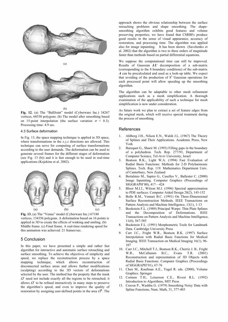
(a)

(b)

Fig. 12. (a) The “BallJoint” model (Cyberware Inc.) 34267 vertices, 68530 polygons. (b) The model after smoothing based on 15-point interpolation (the surface variation σ < 0.3). Processing time: 4.9 sec.

4.3 Surface deformation

In Fig. 13, the space mapping technique is applied in 3D space, where transformations in the x,y,z directions are allowed. This technique can serve for computing of surface transformations according to the user demands. The deformation can be used to generate several frames for the different stages of deformation (see Fig. 13 (b)) and it is fast enough to be used in real-time applications (Kojekine et al. 2002).

(a) (b) (c) Fig. 13. (a) The “Venus” model (Cyberware Inc.) 67180 vertices, 134356 polygons. A deformation based on 16 points is applied in 3D to create the effects of winking and smiling. (b) Middle frame. (c) Final frame. A real-time rendering speed for this animation was achieved: 21 frames/sec. 5 Conclusion

In this paper, we have presented a simple and rather fast algorithm for interactive and automatic surface retouching and surface smoothing. To achieve the objectives of simplicity and speed, we replace the reconstruction process by a space mapping technique, which allows reconstruction of disconnected surface areas and allows further modifications (sculpting) according to the 3D vectors of deformations selected by the user. The method has the property that the mask Ω+ need not include exactly all the regions to be retouched; it allows Ω+ to be refined interactively in many steps to preserve the algorithm’s speed, and even to improve the quality of restoration by assigning user-defined points in the area ΩR. The

approach shows the obvious relationship between the surface retouching problems and shape smoothing. The shape-smoothing algorithm exhibits good features and volume preserving properties; we have found that CSRBFs produce good results in the sense of visual appearance, accuracy of restoration, and processing time. The algorithm was applied also for image inpainting. It has been shown (Savchenko et al. 2002) that the algorithm is two to three orders of magnitude faster than methods based on partial differential equations.

We suppose the computational time can still be improved. Results of Gaussian LU decomposition of a sub-matrix (corresponding to the 8 boundary conditions) of the sub-matrix A can be precalculated and used as a look-up table. We expect that avoiding of the production of 83 Gaussian operations for each processed point will allow speeding up the smoothing algorithm.

The algorithm can be adaptable to other mesh refinement applications such as a mesh simplification. A thorough examination of the applicability of such a technique for mesh simplification is now under consideration.

As future work we plan to extract a set of feature edges from the original mesh, which will receive special treatment during the process of smoothing. References 1. Ahlberg J.H., Nilson E.N., Walsh J.L. (1967) The Theory

of Splines and Their Applications. Academic Press, New York

2. Barequet G., Sharir M. (1993) Filling gaps in the boundary of a polyhedron. Tech. Rep. 277/93, Department of Computer Science, Tel-Aviv University, Israel

3. Beatson R.K., Light W.A. (1994) Fast Evaluation of Radial Basis Functions: Methods for 2-D Polyharmonic Splines. Tech. Rep. 119. Mathematics Department Univ. of Canterbury, New Zealand

4. Bertalmio M., Sapiro G., Caselles V., Ballester C. (2000) Image Inpainting. Computer Graphics (Proceedings of SIGGRAPH’00), 417—424

5. Bloor M.I.J., Wilson M.J. (1996) Spectral approximation to PDE surfaces. Computer Aided Design 28(2), 145-152

6. Bolle R.M., Vemuri B.C. (1991) On Three-Dimensional Surface Reconstruction Methods. IEEE Transactions on Pattern Analysis and Machine Intelligence, 13(1), 1-13

7. Bookstein F.L. (1989) Principal Warps: Thin Plate Splines and the Decomposition of Deformations. IEEE Transactions on Pattern Analysis and Machine Intelligence, 11(6), 567-585

8. Bookstein F.L. (1991) Morphometric Tools for Landmark Data. Cambridge University Press

9. Carr J.C., Fright W.R., Beatson R.K. (1997) Surface Interpolation with Radial Basis Functions for Medical Imaging. IEEE Transaction on Medical Imaging 16(1), 96-107

10. Carr J.C., Mitchell T.J., Beatson R.K., Cherrie J. B., Fright W.R., McCallumm B.C., Evans T.R. (2001) Reconstruction and representation of 3D Objects with Radial Basis Functions. Computer Graphics (Proceedings of SIGGRAPH’01), 67-76

11. Chen M., Kaufman A.E., Yagel R. eds. (2000), Volume Graphics. Springer

12. Cormen T.H., Leiserson C.E., Rivest R.L. (1992) Introduction to Algorithms, MIT Press

13. Craven P., Washba G. (1979) Smoothing Noisy Data with Spline Functions, Num. Math, 31, 377-403

32. Litwinovicz P., Williams L. (1994) Animating Images with Drawing. Computer Graphics (Proceedings of SIGGRAPH’94), 409-412

14. Davis J., Marschner S.R., Garr M., Levoy M. (2002), Filling Holes in Complex Surfaces using Volumetric Diffusion, Proceedings of the First International Symposium on 3D Data Processing, Visualization, Transmission

33. Morse B., Yoo T.S., Rheingans P., Chen D.T., Subramanian K.R. (2001) Interpolating Implicit Surfaces from Scattered Surface Data Using Compactly Supported Radial Basis Functions. Proceedings of the Shape Modeling Conference, Genova, Italy, 89-98

15. Desbrun M., Meyer M., Schröder P., Barr A.H. (1999) Implicit Fairing of Irregular Meshes using Diffusion and Curvature Flow. Computer Graphics (Proceedings of SIGGRAPH’99) 33, 317-324

16. Dushon J. (1976) Splines Minimizing Rotation Invariants Semi-norms in Sobolev Spaces. In: Schempp W., Zeller K. eds. Constructive Theory of Functions of Several Variables. Springer-Verlag, 85-100

17. Esedoglu S., Shen J. Image Inpainting by the Mumford-Shah-Euler Model. IMA Preprint 1812, accepted for publication in European Journal for Applied Mathematics

35. Oliveira M.M., Bowen B., McKenna R., Chang Y.S.

(2001) Fast Digital Image Inpainting. Proceedings of the Visualization, Imaging, and Image Processing IASTED Conference, Marbella, Spain, 261-266

34. Ohtake Y., Belyaev A., Seidel H-P. (2003) A Multi-scale Approach to 3D Scattered Data Interpolation with Compactly Supported Basis Functions, Proceedings of SMI’2003 , Soul, Korea

36. Press W.H., Teukolsky S.A., Vetterling T., Flannery B.P. (1997) Numerical Recipes in C. Cambridge University Press

18. Farin G. (1998) Curves and Surfaces for CAGD, Academic Press

37. Sarti A., Malladi R., Sethian J.A. (2001) Computing Missing Boundaries in Images. Proceedings of the Visualization, Imaging, and Image Processing IASTED Conference, Marbella, Spain, 495-500

19. Gousie M.K., Franklin W.R. (1998) Converting elevation contours to a grid. Proceeding of the Eighth International Symposium on Spatial Data Handling (SDH), Vancouver BC, Canada http://www.ecse.rpi.edu/Homepages/wrf

38. Savchenko V., Pasko A., Okunev O., Kunii T. (1995) Function Representation of Solids Reconstructed from Scattered Surface Points and Contours. Computer Graphics Forum 14(4), 181-188

20. George A., Liu J.W.H. (1981) Computer Solution of Large Sparse Positive Definite Systems. Prentice-Hall, Englewood Cliffs, NJ, USA

21. Greiner G. (1994) Surface Construction Based on Variational Principles. In : Laurent P.J. et al. eds. Wavelets, Images and Surface Fitting. AL Peters Ltd., 277- 286

39. Savchenko V., Sedukhin S. (2001) Pattern Dependent Reconstruction of Raster Digital Elevation Models from Contour Maps, VIIP 2001, Proceedings of IASTED International Conference on Visualization, Imaging, and Image Processing, 237-244

22. Hermann T., Kovacs Z., Varady T. (1997) Special applications in surface fitting. In: Strasser W., Klein R., Rau R. eds. Geometric Modeling: Theory and Practice, Springer, 14-31

40. Savchenko V., Schmitt L. (2001) Reconstructing Occlusal Surfaces of Teeth Using a Genetic Algorithm with Simulated Annealing Type Selection. Proceeding of 6th ACM Symposium on Solid Modeling and Application. Michigan, USA, 39-46

23. Hoppe H., DeRose T., Duchamp T., McDonald J., Stuetzle W. (1992) Surface Reconstruction from Unorganized Points, Proceedings of SIGGRAPH’92, 26(2), 79-88

41. Savchenko V., Kojekine N. (2002) An Approach to Blend Surfaces. In: Vince J., Earnshaw R. eds. Advances in Modeling, Animation and Rendering (Proceedings of CGI’02), Springer, 139-150

24. Jennings A. (1966) A Compact Storage Scheme for the Solution of Symmetric Linear Simultaneous Equations. Comput. Journal 9, 281-285

25. Kojekine N., Savchenko V., Senin M., Hagiwara I. (2002) Real-time 3D Deformations by Means of Compactly Supported Radial Basis Functions. Short papers proceedings of Eurographics’ 02, 35-43

42. Savchenko V., Kojekine N., Unno H. (2002) A Practical Image Retouching Method. Proceedings of International Symposium Cyber Worlds’02: Theory and Practice, 480-487. 26. Kojekine N., Savchenko V. (2002) Using CSRBFs for

Surface Retouching, Proceedings of The 2nd IASTED International Conference Visualization, Imaging and Image Processing VIIP2002, 613-618

43. Setian J.A. (1996) Level Set Methods: Evolving Interfaces. In: Geometry, Fluid Mechanics, Computer Vision, and Material Sciences, Cambridge University Press

44. Schneider B. (1998) Geomorphologically Sound Reconstruction of Digital Terrain Surfaces from Contours, Proceedings of 8th Symposium on Spatial Data Handling, Vancouver, Canada, http://www.geo.unizh.ch/~benni

27. Kojekine N., Hagiwara I., Savchenko V. (2003) Software Tools Using CSRBFs for Processing Scattered Data. Computer & Graphics, 27, 311-319

28. Kobbelt L., Campagna S., Vorsatz J., Seidel H-P. (1998) Interactive Multi-Resolution Modeling on Arbitrary Meshes. Computer Graphics (Proceedings of SIGGRAPH’98) 32, 105-114

45. Skaria S., Akleman E., Parke F.I. (2001) Modeling Subdivision Control Meshes for Creating Cartoon Faces. Proceedings of the International Conference on Shape Modeling and Applications, Genova, Italy, 216-225 29. Lee S., Chwa K.-Y., Hahn J., Shin S.Y., Wolberg G.

(1995) Image Morphing Using Snakes and Free-Form Deformations. Proceedings of SIGGRAPH`95, 439-448

46. Taubin G. (1995) A Signal Processing Approach to Fair Surface Design. Computer Graphics (Proceedings of SIGGRAPH’95) 29, 351-358 30. Lee S., Wolberg G., Shin S.Y. (1997) Scattered Data

Interpolation with Multilevel B-Splines. IEEE Transactions on Visualization and Computer Graphics 3(3), 228-244

47. Turk G., Levoy M. (1994) Zippered Polygon Meshes from Range Images. Computer Graphics (Proceedings of SIGGRAPH’94), 311-318

31. Light W. (1994) Using Radial Functions on Compact Domains. In: P. J. Laurent et al. eds. Wavelets, Images and Surface Fitting. AL Peters Ltd., 351-370

48. Turk G., O’Brien J.F. (1999) Shape Transformation Using Variational Implicit Functions. Computer Graphics (Proceedings of SIGGRAPH’99), 335-342

49. Vasilenko V.A. (1983) Spline-functions: Theory, Algorithms, Programs. Nauka Publishers, Novosibirsk

50. Warren J., Weimer H. (2002) Subdivision Methods for Geometric Design, Academic Press

51. Wendland H. (1995), Piecewise polynomial, positive definite and compactly supported radial functions of minimal degree. Adv. in Comput. Math. 4, 389-396

52. Wendland H. (1999) On the smoothness of positive definite and radial functions. Journal of Computational and Applied Mathematics 101, 177-188

53. Whitaker R.T., Breen D.E. (1998) Level-set Models for the Deformation of Solid Objects, Proceedings of Implicit Surfaces Conference, 19-35

54. Wyvill B., Van Overveld K. (1997) Warping as a Modeling Tool for CSG/Implicit Models. Proceedings of the International Conference on Shape Modeling and Applications, 205-213

55. Yagou H., Belyev A., Wei D. (2002) Mesh Median Filter for Smoothing 3-D Polygonal Surfaces. Proceedings of CW’02

56. Yagou H., Ohtake Y, Belyev A. (2003) Mesh Denosing via Iterative Alpha-Trimming and Nonlinear Diffusion of Normals with Automatic Thresholding, CGI`2003

57. Zhang H., Fiume E. (2002), Mesh Smoothing with Shape or Feature Preservation. In: Vince J., Earnshaw R. eds. Advances in Modeling, Animation and Rendering (Proceedings of CGI’02). Springer, 167-181