Embed Size (px)
Citation preview
AN EFFECTIVENESS EVALUATION METHOD FOR AIRBURST PROJECTILES
A THESIS SUBMITTED TO THE GRADUATE SCHOOL OF NATURAL AND APPLIED SCIENCES
OF MIDDLE EAST TECHNICAL UNIVERSITY
BY
OKTAY SAYGIN
IN PARTIAL FULLFILLMENT OF THE REQUIREMENTS FOR
THE DEGREE OF MASTER OF SCIENCE IN
ELECTRICAL AND ELECTRONICS ENGINEERING
MAY 2011
Approval of the thesis:
AN EFFECTIVENESS EVALUATION METHOD FOR AIRBURST PROJECTILES
submitted by OKTAY SAYGIN in partial fulfillment of the requirements for the degree of Master of Science in Electrical and Electronics Engineering Department, Middle East Technical University by,
Prof. Dr. Canan Özgen Dean, Graduate School of Natural and Applied Sciences Prof. Dr. Đsmet Erkmen Head of Department, Electrical and Electronics Engineering Prof. Dr. Erol Kocaoğlan Supervisor, Electrical and Electronics Engineering Dept., METU
Examining Committee Members: Prof. Dr. Mübeccel Demirekler Electrical and Electronics Engineering Dept., METU Prof. Dr. Erol Kocaoğlan Electrical and Electronics Engineering Dept., METU Prof. Dr. Kemal Leblebicioğlu Electrical and Electronics Engineering Dept., METU Asst. Prof. Dr. Afşar Saranlı Electrical and Electronics Engineering Dept., METU Dr. Hüseyin Yavuz ASELSAN Inc.
Date:

iii
I hereby declare that all information in this document has been obtained and presented in accordance with academic rules and ethical conduct. I also declare that, as required by these rules and conduct, I have fully cited and referenced all material and results that are not original to this work.
Name, Last name : Oktay SAYGIN
Signature :
iv
ABSTRACT
AN EFFECTIVENESS EVALUATION METHOD FOR AIRBURST PROJECTILES
Saygın, Oktay
M. S., Department of Electrical and Electronics Engineering
Supervisor: Prof. Dr. Erol Kocaoğlan
May 2011, 67 pages
Airburst projectiles increase the effectiveness of air defense, by forming clouds of
small pellets. In this work, in order to evaluate the effectiveness of airburst
projectiles, Single Shot Kill Probability (SSKP) is computed at different burst
distances by using three lethality functions defined from different measures of
effectiveness. These different measures are target coverage, number of sub-projectile
hits on the target and kinetic energy of sub-projectiles after burst. Computations are
carried out for two different sub-projectile distribution patterns, namely circular and
ring patterns. In this work, for the determination of miss distance, a Monte Carlo
simulation is implemented, which uses Modified Point Mass Model (MPMM)
trajectory equations. According to the results obtained two different distribution
patterns are compared in terms of effectiveness and optimum burst distance of each
distribution pattern is determined at different ranges.
Keywords: Airburst Projectile, Burst Distance, Target Coverage, Single Shot Kill
Probability (SSKP)
v
ÖZ
HAVADA PARALANAN MÜHĐMMATLAR ĐÇĐN BĐR ETKĐNLĐK DEĞERLENDĐRME METODU
Saygın, Oktay
Yüksek Lisans, Elektrik Elektronik Mühendisliği Bölümü
Tez Yöneticisi : Prof. Dr. Erol Kocaoğlan
Mayıs 2011, 67 sayfa
Havada paralanan mühimmatlar, küçük parçacık bulutları oluşturarak hava savunma
etkinliğini arttırırlar. Bu çalışmada, havada paralanan mühimmatların etkinliğini
değerlendirmek için, farklı etkinlik parametrelerinden tanımlanan üç hasar
fonksiyonu kullanılarak, farklı paralanma mesafelerinde tek atım yok etme olasılığı
hesaplanmıştır. Bu etkinlik parametreleri hedef kaplaması, hedefe vuran parçacık
sayısı ve parçacıkların paralanma sonrası kinetik enerjileridir. Hesaplamalar daire ve
halka şekilleri olarak adlandırılan iki farklı parçacık dağılım şekline göre
gerçekleştirilmiştir. Bu çalışmada, kaçırma mesafesini belirlemek üzere Modified
Point Mass Model (MPMM) yörünge denklemlerini kullanan bir Monte Carlo
benzetimi uygulanmıştır. Elde edilen sonuçlara göre iki farklı dağılım şekli etkinlik
açısından karşılaştırılmış ve her bir dağılım şekli için farklı menzillerde en iyi
paralanma mesafesi belirlenmiştir.
Anahtar Kelimeler: Havada Paralanan Mühimmat, Paralanma Mesafesi, Hedef
Kaplaması, Tek Atım Yok Etme Olasılığı

vi
To My Love

vii
ACKNOWLEDGEMENTS
I would like to express my sincere thanks and gratitude to my supervisor Prof. Dr.
Erol Kocaoğlan for his complete guidance, advice and criticism throughout this
study.
I am grateful to my manager Dr. Hüseyin Yavuz for his participation in the
committee, his valuable comments and suggestions about the thesis.
I would like to thank my colleagues in ASELSAN Inc. for their support and I would
like express my special thanks to Özdemir Gümüşay and Đnci Yüksel for their
guidance and advice throughout my study.
I would like to thank ASELSAN Inc. for providing me a peaceful working
environment and resources.
I would like to express my special appreciation to my wife for her belief and
encouragements.
viii
TABLE OF CONTENTS
ÖZ ................................................................................................................................ v
ACKNOWLEDGEMENTS ....................................................................................... vii
TABLE OF CONTENTS .......................................................................................... viii
LIST OF FIGURES ..................................................................................................... x
LIST OF TABLES ..................................................................................................... xii
CHAPTERS……..........................................................................................................1
1 INTRODUCTION ............................................................................................... 1
1.1 Background and Motivation .......................................................................... 1
1.2 Outline of The Thesis .................................................................................... 2
2 AIRBURST PROJECTILES ................................................................................ 4
2.1 Different Distribution Patterns ...................................................................... 7
3 RANDOM ERRORS ......................................................................................... 10
3.1 Delivery Errors ............................................................................................ 12
3.2 Mathematical Modeling of Random Errors ................................................. 13
3.3 Single Shot Kill Probability ........................................................................ 15
3.4 Determination of Standard Deviations of Burst Point ................................. 17
3.4.1 Trajectory Model .................................................................................. 18
3.4.2 Monte Carlo Simulation ....................................................................... 25
4 METHODOLOGY ............................................................................................. 32
4.1 Expected Coverage Area Computation ....................................................... 32
4.2 Expected Number of Sub-projectile Hits Computation .............................. 37
4.3 Analysis of Different Measures of Effectiveness ........................................ 38
4.3.1 Target Coverage ................................................................................... 40
4.3.2 Number of Sub-projectile Hits ............................................................. 43
4.3.3 Maximum Effectiveness....................................................................... 46
4.3.4 Kinetic Energy of Sub-projectiles ........................................................ 51
4.4 Single Shot Hit Probability Computation .................................................... 52

ix
4.5 Single Shot Kill Probability Computation ................................................... 55
5 CONCLUSION .................................................................................................. 64
REFERENCES ........................................................................................................... 66
x
LIST OF FIGURES
FIGURES
Figure 2.1: Burst angle representation ......................................................................... 5
Figure 2.2: Circular distribution pattern....................................................................... 8
Figure 2.3: Ring distribution pattern ............................................................................ 9
Figure 3.1: Miss distance representation .................................................................... 11
Figure 3.2: Mean Point of Impact (MPI) ................................................................... 13
Figure 3.3: Normal probability density function........................................................ 14
Figure 3.4: Schematic top and side views of projectile firing.................................... 29
Figure 4.1: Bivariate normal distribution of burst points ........................................... 33
Figure 4.2: Coverage area representation................................................................... 34
Figure 4.3: Coverage area computation ..................................................................... 36
Figure 4.4: Relation between burst angle and burst distance ..................................... 39
Figure 4.5: Target coverage for circular pattern ........................................................ 40
Figure 4.6: Target coverage for different r2/ r1 ratios for ring pattern ........................ 41
Figure 4.7: Target coverage for ring pattern with r2/ r1 ratio of ½ ............................. 42
Figure 4.8: Number of sub-projectile hits for circular pattern ................................... 43
Figure 4.9: Number of sub-projectile hits for different r2/ r1 ratios for ring pattern .. 44
Figure 4.10: Number of sub-projectile hits for ring pattern with r2/ r1 ratio of ½ ...... 45
Figure 4.11: Maximum effectiveness for circular pattern .......................................... 47
Figure 4.12: Maximum effectiveness for different r2/ r1 ratios for ring pattern ......... 48
Figure 4.13: Maximum effectiveness for ring pattern with r2/ r1 ratio of ½............... 50
Figure 4.14 : Hit and no hit condition for airburst projectiles ................................... 52
Figure 4.15: PH vs. burst distance for circular pattern ............................................... 53

xi
Figure 4.16: PH vs. burst distance for ring pattern with r2/ r1 ratio of ½ .................... 54
Figure 4.17: Lethality due to target coverage ............................................................ 57
Figure 4.18: Lethality due to number of sub-projectiles ............................................ 58
Figure 4.19: Lethality due to kinetic energy of a sub-projectile ................................ 59
Figure 4.20: PK vs. burst distance for circular pattern ............................................... 61
Figure 4.21: PK vs. burst distance for ring pattern ..................................................... 62
xii
LIST OF TABLES
TABLES
Table 3-1: Standard deviations of random errors ....................................................... 25
Table 3-2: Input values to MPMM............................................................................. 28
Table 3-3: Nominal azimuth and elevation distances ................................................ 29
Table 3-4: Azimuth and elevation standard deviations of miss distance ................... 30
Table 4-1: Burst distances of maximum target coverage ........................................... 43
Table 4-2: Results for circular pattern ....................................................................... 47
Table 4-3: Optimum burst distances for different r2/ r1 ratios for ring pattern .......... 49
Table 4-4: Results for ring pattern ............................................................................. 50
Table 4-5: Nominal speeds for projectile ................................................................... 51
Table 4-6: Kinetic energy of a sub-projectile ............................................................ 52
Table 4-7: Peak PH values and burst distances for ring pattern ................................. 55
Table 4-8: Peak PK values and optimum burst distances for circular pattern ............ 61
Table 4-9: Peak PK values and optimum burst distances for ring pattern .................. 63
1
CHAPTER 1
INTRODUCTION
1.1 Background and Motivation
The general air defense problem is to bring a sufficiently large destructive potential
at the right time to the instantaneous position of the target to be combated. The
custom inputs that are taken for any fire control system are target related properties
(i.e. position and velocity), projectile related properties (i.e. mass, geometry, initial
velocity, initial spin rate) and environmental properties which are gravity, and
atmospheric conditions.
In the simplest instance, the destructive potential for a ballistic projectile is kinetic
energy. These projectiles are ineffective against fast moving and small sized targets
due to errors like meteorological variations and ballistic dispersion of both weapon
and projectile. In order to increase the effectiveness of air defense against these
targets, it is a practical solution to utilize airburst projectiles. Airburst projectiles
increase the effectiveness by forming clouds of small pellets in front of the target
trajectory.
There are many criteria for effectiveness evaluation of airburst projectiles such as
burst distance and time of burst. In order to determine optimum burst distance for an
airburst projectile, an optimization of a cost function is done in [1]. In that work, the
variables of the objective function are target coverage, number of sub-projectile hits
on the target, and hit velocity of sub-projectiles to target. The effects of several
factors such as target range, target dimension, firing angle on burst distance are
analyzed. The variables of the objective function in that work are also used in the
scope of this work. In [2], the time of burst is optimized in order to increase the
2
effectiveness of time programmable airburst projectiles. The time of burst is
determined according to a predetermined distance. On the other hand, in [3], a
method is proposed in order to increase the effectiveness of air defense for a
remotely programmable airburst projectile. After projectile is fired target is
continued to be tracked during the flight of the projectile. With the better known
target position, the projectile is burst accordingly, and the effectiveness of the
projectile is increased.
In this work, the criteria of burst distance is used for effectiveness evaluation of
airburst projectiles. Because with increasing burst distances target coverage increases
but number of sub-projectile hits decreases, therefore, there should be optimum
values of effectiveness and burst distances that should be found out.
1.2 Outline of The Thesis
The outline of the thesis is as follows:
In Chapter 2, the concept of airburst projectiles is explained. The descriptions of the
two types of airburst projectiles, which differ according to their sub-projectile
distribution, are given in this chapter.
In Chapter 3, delivery errors resulting from different sources of fire control elements
are described. The expressions related to mathematical modeling of random errors
and to Single Shot Kill Probability (SSKP) computation are given. The details of
trajectory model utilized are explained with the related equations of motion. Then,
Monte Carlo simulation implemented in order to determine miss distance is
explained.
In Chapter 4, the methodology applied in order to evaluate the effectiveness of
airburst projectiles is given. Three measures of effectiveness of airburst projectiles,
which are target coverage, number of sub-projectile hits on the target and kinetic
energy of sub-projectiles after burst, are analyzed and single shot hit and kill
probabilities, are computed for two different distribution patterns. From the results of

3
analysis and computation, optimum burst distances are determined for each different
distribution pattern.
In Chapter 5, two different distribution patterns are compared in terms of
effectiveness. The thesis is concluded with the evaluations of the results obtained,
and some recommendations on future work concerning effectiveness evaluation for
airburst projectiles.
4
CHAPTER 2
AIRBURST PROJECTILES
There are multiple ways of increasing the effectiveness of barreled air defense
weapon systems. One way is to fire multiple projectiles to the same target at the
same time. This can be done by the same weapon system or from different weapon
systems. On the contrary, the probability of hitting the target can sometimes be
increased by firing the weapons in a pattern around the target, rather than directly on
it. Due to errors common to all shots, it might not be the best to fire all weapons at
the same time directly to the same target in a multiple projectile shot [4]. This
observation leads naturally to the problem of finding the optimal pattern. However,
in pattern firing there is an aim point selection and the firings does not have the same
aim point in order to satisfy high damage against targets.
Besides, using airburst projectiles is another solution for increasing the effectiveness
of barreled air defense weapon systems against fast and small targets. Airburst
projectiles utilize sub-projectiles and form a cloud of small pellets which increases
the probability of hit.
The concept of airburst projectile is based on the ejection of the sub-projectiles at a
pre-calculated point, which is called “burst point”. Airburst projectiles burst at a
distance d in front of the target. Fire control system determines the time of burst of
the projectile to eject its sub-projectiles in front of the future target position. After
burst point, the sub-projectiles move towards the target in a conical or similar shape
and make a sub-projectile cloud which is in tens or hundreds at the same time on the
same target.
The method of activation to eject sub-projectiles is determined by the type of fuze.
Using a projectile with proximity fuze may be one solution for ejection. With the
signal processing taking place inside the projectile, this type of fuze bursts the
5
projectile and ejects its sub-projectiles in close distance to the target. Another
solution is using time fuze. For this type, weapon system calculates a time of burst
within very short duration and transfers this data before projectile leaves the weapon.
The projectile counts down this time during its flight towards target. At the time
when the zero count is reached, time fuze activates the projectile to eject its sub-
projectiles. Then the sub-projectiles are directed towards the target in a conical or
similar shape.
Just before burst, the projectile has a linear velocity in its longitudinal direction, and
an angular velocity around its direction of motion, due to its spinning. With the linear
and radial velocity components, sub-projectiles move towards the target in a conical
envelope. The magnitudes of velocity components determine the angle of this conical
volume. If the magnitude of radial velocity increases relative to linear velocity, burst
angle α increases. (Figure 2.1)
Figure 2.1: Burst angle representation
6
Time of burst of an airburst projectile is flight time of the projectile to the ideal
impact point less a lead time, which should be determined optimally on the basis of
the conditions at the time. The lead time determines the distance d between burst
point and instantaneous target position.
In order to cover the uncertainties of both the projectile position, and target positions,
this distance should be high. However, in order to deliver a sufficient kinetic energy
on the target area this distance should be small which results in higher number of
sub-projectiles hit on the target and high penetration capabilities. Therefore, for the
effectiveness evaluation of airburst projectiles, there are many criteria that should be
considered. These criteria are as follows:
• Number of sub-projectiles inside a single projectile
• Mass of each sub-projectile
• Geometry and installation of sub-projectiles (form-fit factor)
• Burst angle of projectile
• Burst distance of projectile from the target
Increasing the number of sub-projectiles inside a single projectile is going to increase
the effectiveness. Since a projectile has “limited” dimensions and geometry,
increasing the number of sub-projectiles decreases the mass of each sub-projectile.
Therefore, there is a trade-off in terms of effectiveness between the number of
projectiles and the mass of each sub-projectile.
Another criterion is burst angle of projectile and this is related to the spin rate and the
linear velocity of the projectile. With a high burst angle, sub-projectiles can cover a
large area on the target but since the sub-projectiles are scattered in a large volume,
number of sub-projectiles per unit area decreases. On the contrary, with a low burst
angle the number of sub-projectiles per unit area increases but for this time the
coverage area of target decreases. There is again a trade-off in terms coverage and
number of sub-projectile hits on the target. Same situation is valid for burst distance
of projectile from the target. Increasing the distance of burst point from the target,
increases the coverage but decreasing this distance decreases the number of sub-
7
projectile hits on the target. As a result, there should be optimum values of
effectiveness and burst distances that should have to be found out for airburst
projectiles.
Therefore, the geometry of the projectile, number of sub-projectiles inside the
projectile, mass of each sub-projectile and the installation of sub-projectiles inside
the projectile should have to be optimally determined in order to have the best burst
angle for an effective airburst projectile.
In this work, for effectiveness evaluation of airburst projectiles, objective is to
evaluate the effectiveness of airburst projectiles at different burst distances;
• For different types of airburst projectiles
• At different target ranges
• For a representative rectangular target
Different measures of effectiveness for airburst projectiles, such as target coverage
and number of sub-projectile hits are analyzed and Single-Shot Kill Probability
(SSKP) is computed at different burst distances. From the computation results,
optimum burst distances are determined for two different distribution patterns.
2.1 Different Distribution Patterns
In what pattern sub-projectiles move and hit on the target, is dependent on many
factors. These factors are:
• placement of sub-projectiles in the projectile
• geometry of each sub-projectile
• means of releasing the sub-projectiles
• magnitudes of the initial velocity components of sub-projectiles
• environmental conditions
8
Airburst projectiles may differ according to their sub-projectile distribution while
they are moving towards the target. In this work, two different sub-projectiles
distribution is determined. One is circular and the other is ring shaped patterns.
In circular shaped pattern, the sub-projectiles are assumed to be enclosed in a circular
area. As time passes this circular area gets larger and the density of sub-projectiles
decreases. This is because the number of sub-projectiles is constant. At the time of
impact of sub-projectiles on target, the sub-projectile coverage of circular pattern
over a rectangular target is illustrated in Figure 2.2.
Figure 2.2: Circular distribution pattern
Another distribution pattern of sub-projectiles is ring shaped pattern. In this pattern,
sub-projectiles are included in a ring shaped area. As time passes this ring gets larger
and the density of sub-projectiles is decreasing since the number of sub-projectiles is
fixed. Ring pattern has more sub-projectile in the unit area than circular pattern,
while propagating towards target. At the time of hit of sub-projectiles on target, the
sub-projectile coverage of ring pattern over a rectangular target is illustrated in
Figure 2.3. r1 is the outer radius and r2 is the inner radius of the ring pattern.
9
Figure 2.3: Ring distribution pattern
Airburst projectiles defeat their target with their kinetic energy. With the burst of
projectile, this kinetic energy is transferred to the sub-projectiles with respect to the
conservation of energy principle. Sub-projectiles carry this total kinetic energy of
projectile to the target. The only difference being in the manner how they carry this
potential of damage. These two different distribution patterns have different densities
according to their distribution of sub-projectiles. Circular pattern carries in a lighter
density than ring pattern since it has larger area of propagation [3].
10
CHAPTER 3
RANDOM ERRORS
Main purpose of a weapon system is to be effective against a target in order to
prevent its purpose of attack. Fire control system determines azimuth and elevation
orientation angles of the weapon pointing by taking into account the following inputs
or data:
• Target velocity
• Weapon system velocity on which the barrels are installed
• Projectile ballistics
• Meteorological data
However, fire control systems cannot control all the errors resulting from different
sources such as target position determination, weapon aiming errors, etc. There is
always a difference between the predicted hit point and actual hit point and this
difference is called “miss distance”. Miss distance can be separated into two
components; one is in azimuth direction and the other is in elevation direction.
(Figure 3.1)
11
Figure 3.1: Miss distance representation
The main sources of miss distance in elevation direction due to projectile ballistics
are:
• Variations in projectile mass
• Muzzle velocity variations
• Front/Tail wind
• Air density
• Air temperature
Additionally, the main sources of miss distance in azimuth direction due to projectile
ballistics are:
• Muzzle velocity variations
• Lateral wind
12
• Gyroscopic effects resulting from the spin of the projectile
Fire control system estimates the future target position. However, since there are
natural variances in the estimation algorithms and delay between measured target
position and actual target position there is an error called “target position error”.
Weapon pointing errors and target position errors cause delivery of projectile to a
different point from actual target position. These errors are called aiming errors
which are also known as bias errors [5].
3.1 Delivery Errors
Generally, delivery errors result from different sources of fire control elements. They
can be decomposed into two as aiming and dispersion errors.
Aiming errors, sometimes called bias errors, are common to all firings which may be
the result of gun orientation errors, target position errors, etc. On the other hand,
dispersion is a measure how the projectiles differ from the Mean Point of Impact
(MPI) which is the point whose coordinates are the arithmetic means of the
coordinates of the separate impact points of a finite number of projectiles fired at the
same aiming point under a given set of conditions. Dispersion is the result of random
factors such as meteorological variations, weapon and projectile ballistic dispersion.
These errors cause distribution of impact points around MPI. For a burst of five
projectiles MPI, aiming error and dispersion of each projectile shot around MPI are
shown in Figure 3.2.
13
Figure 3.2: Mean Point of Impact (MPI)
Dispersion type of errors are sometimes called precision errors resulting from the
muzzle velocity variations of the projectile, meteorological disturbances such as
tail/front wind and the projectile dispersion properties due to manufacturing
tolerances. Dispersion errors are random and they are expressed mathematically with
probability density functions.
3.2 Mathematical Modeling of Random Errors
Random errors need to be accounted for in mathematical models for effectiveness
considerations. Errors cause a projectile to impact at a different point from predicted
hit point. Random errors are probabilistic and they can be defined with probability
density functions. The custom assumption for random errors in any fire control
problem is to taking them as normal probability density function. These errors occur
in azimuth and elevation directions. Then, they can be assumed as bivariate normal
probability density function with its variants independency. Probability density
function for normal distribution is expressed with Equation (3-1).
14
p�x� � 1√2πσ� e������������
(3-1)
where
µx: The mean value of distribution in x direction
σx: The standard deviation value of distribution in x direction
Normal probability density function is given in Figure 3.3 with the representation of
mean and standard deviation. Aiming errors and target position errors are treated as
mean and the other errors are treated as standard deviation of the distribution.
Figure 3.3: Normal probability density function
For bivariate normal distribution to characterize probability distributions of delivery
errors with the assumption of independency, probability density function can be
defined as the multiplication of each variants in x and y directions. (Equation (3-2))
15
p�x, y� � p�x�p�y� � 12πσ�σ� e������������� � ����������� �
(3-2)
where
µx: The mean value of distribution in x direction
σx: The standard deviation value of distribution in x direction
µy: The mean value of distribution in y direction
σy: The standard deviation value of distribution in y direction
x and y denote the directions of the specified mean and standard deviation. The
elevation direction is denoted by y and the azimuth direction is denoted by x.
To measure the effectiveness, fundamental military requirement imposed on a
weapon system is the probability of kill. This measure varies according to weapon
system considered since the mechanisms and projectiles used for weapon systems
differ from one to another.
In this work, the general effectiveness evaluation of airburst projectiles is Single Shot
Kill Probability (SSKP).
3.3 Single Shot Kill Probability
Single Shot Kill Probability (SSKP) is a performance value of damage that can be
given to a target by a projectile. SSKP is defined as the product of three performance
measures;
PK � PH x PR x PL
(3-3)
16
"# is the probability that a projectile hits the target, "$ is the probability that the
system works correctly, "% is the probability that a specified level of damage is
achieved which is usually called lethality. This measure is the conditional probability
of a kill, given hit. In this work, the measure "$ (reliability) is not considered since
the system reliability is out of the scope of this study and therefore; "$ is assumed to
be equal to 1 for all computations.
"# is a measure of accuracy for a weapon system. When it is assumed that the
delivery errors have the characteristic behavior of bivariate normal distribution with
variants independency, "# for a shot-target combination is evaluated according to
Equation (3-4). [6]
PH � 12πσxσy & e '(�x'μx�22σx2 * +y'μy,2
2σy2 -dA
(3-4)
where
A: The target area of integration
"% is lethality measure and it is represented by lethality functions. Let ( )yxl , be a
lethality function or damage function denoting the probability of target destruction
when the projectile impact point is at ( )yx, where x is the distance in azimuth, y is
the distance in elevation relative to predicted aim point. Then, ( )yxl , represents the
likelihood of target destruction when impact point is ( )yx, .
When actual impact point of a single projectile is at ( )yx, and denoted lethality
function is expressed as ( )yxl , then Single-Shot Kill Probability (SSKP) can be
expressed by Equation (3-5), where the expression for ( )yxp , is given by Equation
(3-2).
17
PK � & & l�x, y�p�x, y�dxdy∞'∞
∞'∞
(3-5)
In order to evaluate the effectiveness of an air defense weapon system, basic
measures are hit and kill probabilities. Hit probability measures success on the
likelihood of scoring just a hit on the target but kill probability is a comprehensive
measure and dependent on many factors: [7]
• Detailed knowledge of position of impact on target
• Size, mass, and impact velocity of projectile or fragment striking target
• Vulnerability characteristics of the various elements of the target
In this work, in order to evaluate the effectiveness of airburst projectiles Single Shot
Kill Probability (SSKP) is computed. For SSKP computation, three lethality
functions related to target coverage, number of sub-projectile hits on the target and
kinetic energy of sub-projectiles after burst, are determined. However, target
vulnerability characteristics are not considered in the scope of this work.
3.4 Determination of Standard Deviations of Burst Point
In order to evaluate the effectiveness of airburst projectiles, standard deviations of
projectile both in azimuth and elevation directions should be determined. In this
work, a Monte Carlo simulation is implemented which determines the effects of three
distinct random errors. These errors are projectile and weapon ballistics dispersion,
muzzle velocity variation and wind speed variation. This simulation utilizes a
comprehensive trajectory model, namely Modified Point Mass Model (MPMM). The
details of the trajectory model, Monte Carlo simulation implemented and the results
for standard deviations of miss distances on the target plane are given in the
following sections.
18
3.4.1 Trajectory Model
There are simple ways of modeling the trajectory of a projectile such as zero drag, 2
Degree of Freedom (DoF) point mass models. For zero drag models only the gravity
term and for 2DoF point mass models the gravity and drag terms are taken into
account [8]. Moreover, there is another ballistic trajectory model which is used by
NATO Armaments Ballistics Kernel (NABK) trajectory program. This program
implements Modified Point Mass Model (MPMM) in order solve the fire control
problem for spin stabilized projectiles. Contrary to simple ballistic trajectory models,
in MPMM lift force, magnus force, and the coriolis acceleration are included in the
acceleration equations, making MPMM computationally intensive [8].
In this thesis, MPMM is the fundamental trajectory model utilized to derive standard
deviations of miss distance of projectile in azimuth and elevation directions. To
derive an MPMM trajectory model is out of the scope of this study. The model is
taken from ASELSAN resources, which is only used to determine miss distances.
The equations related to MPMM is basically derived from Newton’s Second Law of
Motion which gives the expression of acceleration applied to a object in terms of its
mass and force applied to the object. That is, the ratio of force applied to the object
and mass of the object gives the acceleration.
F34 � mu347
(3-6)
where
84: Net force vector applied to the object
:: Mass of the object
u347 : Acceleration vector of the object
19
In MPMM the net force applied to a spin stabilized projectile is given according to
Newton Second Law of Motion.
F34 � mu347 � DF33334 * LF33334 * MF333334 * mg4 * m >34
(3-7)
where:
?8333334: Drag force vector
@833334: Lift force vector
A83333334: Magnus force vector
:B4: Gravitational force vector
: >334: Coriolis force vector
The evaluation of each term given above is not trivial and the expressions for each
are obtained from NATO Standardization Agreement 4355 (NATO-STANAG 4355)
[9].
While a ballistic projectile moves in the atmosphere there is going to be an opposing
force which is called air drag. Air drag is dependent on the velocity of the projectile
with respect to air. Air drag mostly affects the desired range of the projectile to be
achieved since it opposes the direction of the velocity vector. The acceleration due to
air drag force is given according to Equation (3-8).
DF33334m � ' Cπρid2
8m G HCD,0 * CD,α2�QDαe�2 * CD,α4�QDαe�4N vv4
(3-8)
ρ: Density of air (PB :QR )
20
S: Quadrant elevation fitting form factor
d: Reference diameter of projectile (:)
m: Mass of projectile (PB)
CT,U: Zero yaw drag force coefficient
CT,V�: Quadratic drag force coefficient (1 WXY�R )
QT: Yaw drag fitting factor
CT,VZ: Quartic drag force coefficient (1 WXY[R )
v: Speed of projectile (: \⁄ )
v34: Velocity of projectile with respect to air (: \⁄ )
One way for stabilizing the projectile during its flight is spinning. For a projectile
spinning in the clockwise direction, an upward force during its flight causes the nose
of the projectile yawing to the right. The angle of this yaw is known as the “Yaw of
Repose and is caused by the gyroscopic reaction of the projectile to the vertical
angular rate as the projectile tracks the trajectory curvature causing the projectile to
generate a yaw angle in the horizontal plane” [10]. The expression of yaw of repose
is given by Equation (3-9).
αe3334 � 8Ixp�v4 x u34_ �πρd3�CM,α * CM,α3αe2�v4
(3-9)
p: Axial spin rate of projectile (WXY \R )
I�: Axial moment of inertia (PB :�)
u34_ : Acceleration of center of mass in the fixed coordinate system (: \�R )
21
Ca,V: Overturning moment coefficient
Ca,Vb: Cubic overturning moment coefficient (1 WXY�R )
αe0333334 � �000�
(3-10)
is the initial value of yaw of repose.
The projectile moves in air during its flight. Air moves at differing velocities over the
upper and lower portions of the projectile. This difference in air velocity creates a
pressure differential that imparts a corresponding force to the projectile known as
“dynamic lift” [11].The acceleration due to lift force is given by Equation (3-11).
LF33334m � Cπρd2fL8m G dCL,α * CL,α3αe2 * CL,α5αe4 fv2αe3334
(3-11)
fg: Lift factor
Cg,V: Lift force coefficient (1 WXYR )
Cg,Vb: Cubic lift force coefficient (1 WXYQR )
Cg,Vh: Quintic lift force coefficient (1 WXYiR )
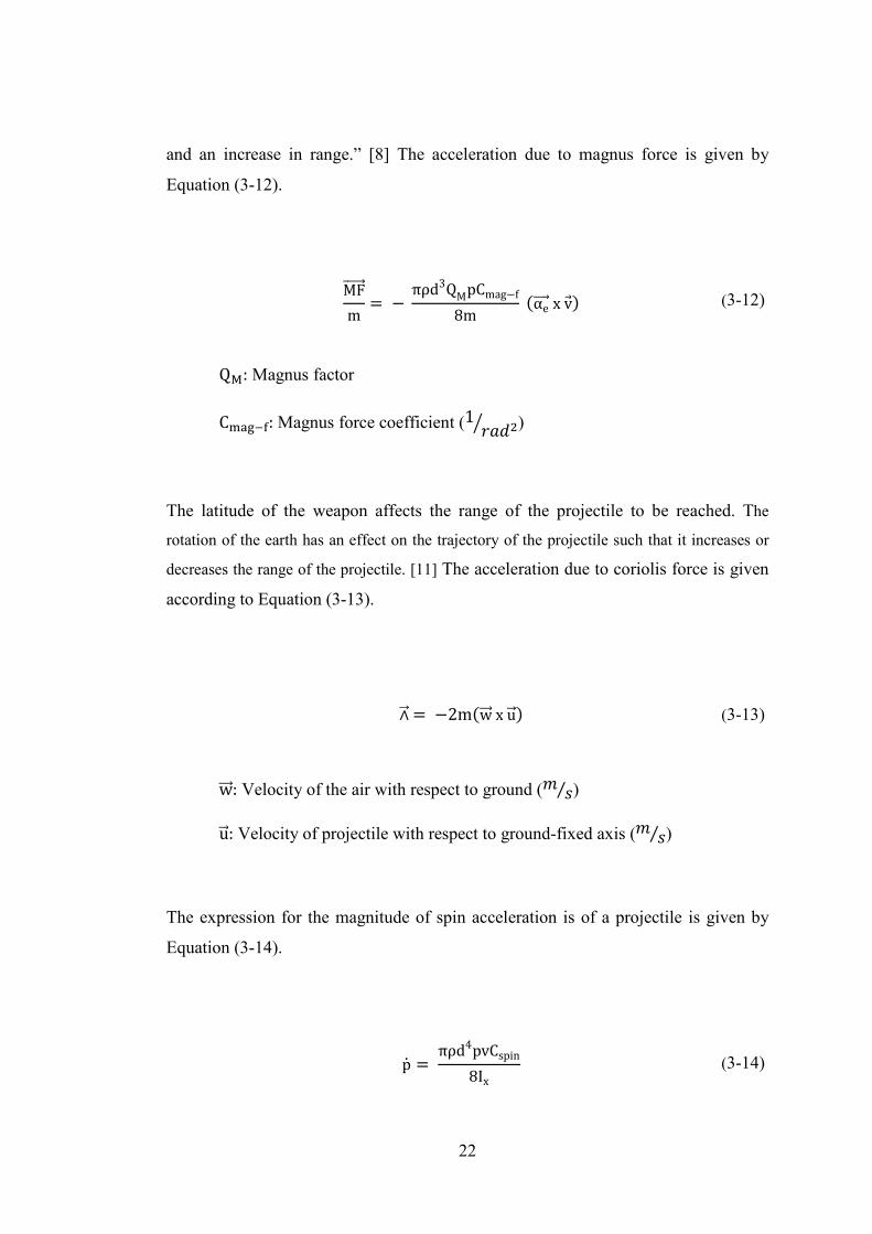
“The Magnus effect is the physical phenomenon where the rotation of a projectile
affects its trajectory when travelling through a fluid. The higher velocity above a
rotating body indicated by the closer streamlines is reflected by a reduction in
pressure. On the other hand, the lower velocity underneath the rotating body has a
higher pressure. The net effect of these pressure changes produces a lift on the body
22
and an increase in range.” [8] The acceleration due to magnus force is given by
Equation (3-12).
MF333334m � ' πρd3QMpCmag'f8m �αe3334 x v4�
(3-12)
Qa: Magnus factor
Cklm�n: Magnus force coefficient (1 WXY�R )
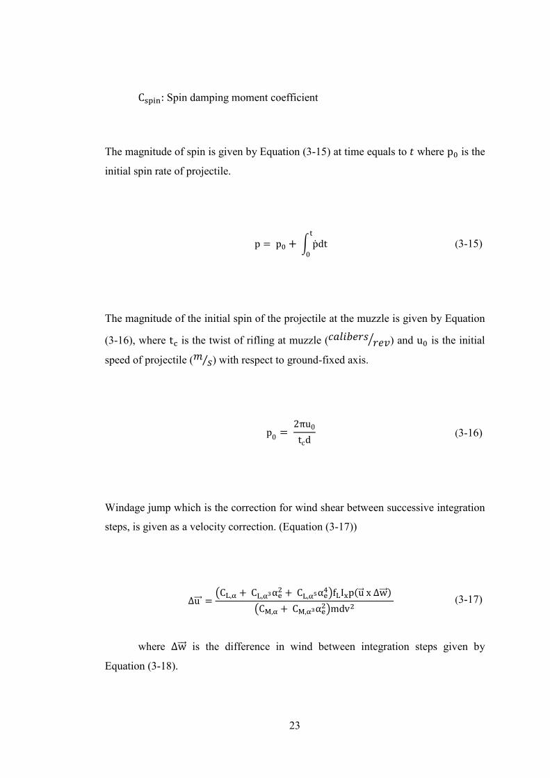
The latitude of the weapon affects the range of the projectile to be reached. The
rotation of the earth has an effect on the trajectory of the projectile such that it increases or
decreases the range of the projectile. [11] The acceleration due to coriolis force is given
according to Equation (3-13).
>34 � '2m�w334 x u34�
(3-13)
w3334: Velocity of the air with respect to ground (: \⁄ )
u34: Velocity of projectile with respect to ground-fixed axis (: \⁄ )
The expression for the magnitude of spin acceleration is of a projectile is given by
Equation (3-14).
p_ � πρd4pvCspin8Ix
(3-14)
23
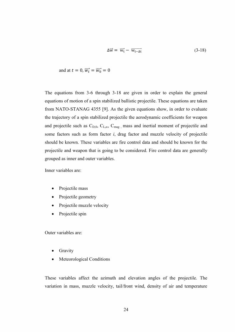
Crstu: Spin damping moment coefficient
The magnitude of spin is given by Equation (3-15) at time equals to v where pU is the
initial spin rate of projectile.
p � pU * & p_ dtxU
(3-15)
The magnitude of the initial spin of the projectile at the muzzle is given by Equation
(3-16), where ty is the twist of rifling at muzzle (zX{S|}W\ W}~R ) and uU is the initial
speed of projectile (: \⁄ ) with respect to ground-fixed axis.
p0 � 2πu0tcd
(3-16)
Windage jump which is the correction for wind shear between successive integration
steps, is given as a velocity correction. (Equation (3-17))
Δu 3334 � �Cg,V * Cg,Vbα�� * Cg,Vhα�[�fgI�p�u34 x Δw3334� �Ca,V * Ca,Vbα���mdv�
(3-17)
where Δw3334 is the difference in wind between integration steps given by
Equation (3-18).
24
Δw3334 � wx33334 ' wx��x333333333334
(3-18)
and at v � 0, ��33334 � �U333334 � 0
The equations from 3-6 through 3-18 are given in order to explain the general
equations of motion of a spin stabilized ballistic projectile. These equations are taken
from NATO-STANAG 4355 [9]. As the given equations show, in order to evaluate
the trajectory of a spin stabilized projectile the aerodynamic coefficients for weapon
and projectile such as CD,0, CL,α, Cmag , mass and inertial moment of projectile and
some factors such as form factor i, drag factor and muzzle velocity of projectile
should be known. These variables are fire control data and should be known for the
projectile and weapon that is going to be considered. Fire control data are generally
grouped as inner and outer variables.
Inner variables are:
• Projectile mass
• Projectile geometry
• Projectile muzzle velocity
• Projectile spin
Outer variables are:
• Gravity
• Meteorological Conditions
These variables affect the azimuth and elevation angles of the projectile. The
variation in mass, muzzle velocity, tail/front wind, density of air and temperature
25
affects the elevation angle. The variations in lateral wind, yaw of repose, coriolis
force affects the azimuth angle of projectile.
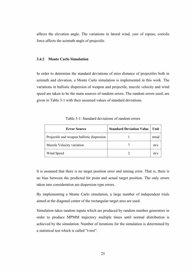
3.4.2 Monte Carlo Simulation
In order to determine the standard deviations of miss distance of projectiles both in
azimuth and elevation, a Monte Carlo simulation is implemented in this work. The
variations in ballistic dispersion of weapon and projectile, muzzle velocity and wind
speed are taken to be the main sources of random errors. The random errors used, are
given in Table 3-1 with their assumed values of standard deviations.
Table 3-1: Standard deviations of random errors
Error Source Standard Deviation Value Unit
Projectile and weapon ballistic dispersion 1 mrad
Muzzle Velocity variation 7 m/s
Wind Speed 2 m/s
It is assumed that there is no target position error and aiming error. That is, there is
no bias between the predicted hit point and actual target position. The only errors
taken into consideration are dispersion type errors.
By implementing a Monte Carlo simulation, a large number of independent trials
aimed at the diagonal center of the rectangular target area are used.
Simulation takes random inputs which are produced by random number generators in
order to produce MPMM trajectory multiple times until normal distribution is
achieved by the simulation. Number of iterations for the simulation is determined by
a statistical test which is called “t-test”.
26
In order to determine the number of replications, a relative precision and confidence
level should be determined. Simulation time depends on the values of these
parameters. Since decreasing relative precision and increasing confidence level
increase the simulation time.
In this work, the relative precision is taken to be 0.1 and 70% confidence interval of
the miss distance in azimuth and elevation is determined. The interval is constructed
such that the half-length of the interval around the mean value is less than or equal to
10% of the calculated mean and the mean value of miss distance is in the calculated
confidence interval with a probability of 0.7. This value is the confidence interval of
1 σ standard deviation of a normal probability distribution. Normal probability
density function is given in Section 3.2.
Random inputs resulting from different sources of errors are simulated with a
normally distributed random number generator in MATLAB environment. The
standard deviations (errors) are used to obtain instantaneous values of the inputs for
MPMM model and azimuth and elevation miss distances for each instance is
recorded. In order to test if the number of replications is enough to characterize a
70% confidence interval with 10% relative precision, t-test is used. If the precision of
the confidence interval is not achieved at the end of replication number of simulation
runs, a new replication number is proposed and simulation runs are taken up to the
proposed replication number. The t-test procedure applied in this work and
summarized above, works as follows [12]:
11.. An initial number of replications � is determined. It is usually chosen to be a
small number like 5, 10 or 20. In this work, this value is taken to be 20.
22.. The results of performance variable are recorded � times which equals the
initial number of replications (z� ’s for 1 � i � n).
33.. The mean of the performance variable is obtained according to Equation
(3-19).
27
Y� � ∑ ctu�n (3-19)
44.. The standard deviation of the performance variable \, which is miss distance
in this work, is obtained according to following equation.
s � �∑ �ct ' Y���u� n ' 1 (3-20)
55.. h is determined according to following equation where α is significance level.
h � t�u���,+��V�, s√n (3-21)
A desired half length �� is calculated using Equation (3-22) with given
desired relative precision W taken to be 0.1.
h� � r Y� (3-22)
66.. If h � h� then simulation stops within confidence interval. ( Y� � h ) 77.. Otherwise,
a. n� � �n + ���,�� * 1 is calculated. Additional ��� ' �� replications
are done.
28
b. Then, �� is taken to be equal to � and the algorithm is repeated to
obtain the results satisfying the determined W and � with the
determined initial number of replications.
Nominal trajectory is the trajectory of the projectile in standard conditions with zero
error. It is needed to obtain miss distances caused from random errors. Thus, miss
distance is taken to be the difference between the nominal trajectory and the
erroneous trajectory. Nominal trajectory is simulated and the position of projectile at
1000 m, 2000 m, and 3000 m ranges are recorded. In order to obtain the nominal
position of projectile at different ranges the basic inputs to MPMM trajectory are
given in Table 3-2.
Table 3-2: Input values to MPMM
Inputs Value
Mass of projectile 1.5 kg
Muzzle velocity of projectile 1000 m/s
Azimuth orientation angle 0°
Elevation orientation angle 45°
Speed of wind 5 m/s
Direction of wind 30°
Weapon orientation angles are taken with respect to weapon reference coordinate
system. On the other hand, direction of wind is taken with respect to earth reference
coordinate system. The schematic view of the firing of projectile with given values in
Table 3-2, is illustrated in Figure 3.4.
29
Figure 3.4: Schematic top and side views of projectile firing
The nominal position of projectile at different ranges is given in Table 3-3, with its
azimuth and elevation positions.
Table 3-3: Nominal azimuth and elevation distances
Range (m) Azimuth Position (m) Elevation Position (m)
1000 0.20 705
2000 0.78 1404
3000 1.80 2098
The random inputs that are taken to obtain the standard deviations are produced by
random number generator. Random number produced for weapon and projectile
ballistic dispersion is added to azimuth orientation and elevation orientation angles of
weapon pointing. Actually, the dispersion value in azimuth is added to azimuth
orientation angle and dispersion value in elevation is added to elevation orientation
angle. The random number produced for muzzle velocity variation is directly added
30
to muzzle velocity input of MPMM trajectory model. The random number produced
for wind speed is added to wind vector which is again the input of MPMM trajectory
model.
Numbers of iterations, standard deviations in azimuth and elevation directions are
given, respectively, in Table 3-4 which is determined for ranges of 1000 m, 2000 m,
and 3000 m.
Table 3-4: Azimuth and elevation standard deviations of miss distance
Range (m) Number of Iterations
Azimuth Standard Deviation (m)
Elevation Standard Deviation (m)
1000 2786 0.70 0.82
2000 5377 1.43 1.52
3000 93335 2.14 2.24
From the determination of standard deviations, it can be concluded that with
increasing range, error propagation increases and the standard deviations in azimuth
and elevation increase. Moreover, number of replications increases with increasing
range.
Ballistic dispersion of weapon and projectile are taken to be equal in both azimuth
and elevation then, they have equal contributions to the miss distances in both
directions. Muzzle velocity mostly contributes in elevation. Because azimuth of
weapon orientation angle is 0°, there is no azimuth component of muzzle velocity at
the firing instance. On the other hand, wind speed variation contributes to both the
azimuth and elevation miss distances. In fact, the lateral wind component contributes
to azimuth, but front wind component contributes to elevation miss distance.
In this work, however, analysis of each random error causing azimuth and elevation
miss distances is out of the scope. The effects of different sources of errors can be
determined with an error budget analysis. Moreover, the derived standard deviations
of miss distance of projectile in azimuth and elevation directions at different ranges
31
are assumed to be the standard deviations of burst point of the projectile. These
values of standard deviations are going to be used to analyze the different measures
of effectiveness of airburst projectiles such as target coverage, number of sub-
projectile hits on the target. Moreover, for Single Shot Kill Probability (SSKP)
computation these values are going to be utilized. The details of SSKP computation
and the results obtained are given in Chapter 4.
32
CHAPTER 4
METHODOLOGY
For effectiveness evaluation of airburst projectiles in this work, Single Shot Kill
Probability (SSKP) is computed for two airburst projectiles which differ according to
their sub-projectile distribution patterns, namely circular and ring shaped patterns.
SSKP is computed at different ranges and for different burst distances. Three
effectiveness measures for an airburst projectile to be effective against a target are:
• Target coverage
• Number of sub-projectiles hits on the target
• Kinetic energy of sub-projectiles
From these measures three lethality functions are determined. These functions are
utilized to compute SSKP for airburst projectiles. Computation results are used to
compare the effectiveness and to determine the optimum burst distances of two
different distribution patterns.
4.1 Expected Coverage Area Computation
Airburst projectiles eject their sub-projectiles in front of the target and generally sub-
projectiles are enclosed in a circular area. When burst point is assumed to be at the
center of the pattern, coverage area for an airburst projectile turns out to be a
rectangular and circular intersection area computation.
With the inclusion of the randomness of the burst point with respect to predicted hit
point, expected value of coverage area can be determined. The burst point is assumed
to have a normal distribution both in azimuth and elevation directions and they are
33
assumed to be independent. Moreover, it is assumed that there is no bias error, that
is, the mean values of the distribution are taken to be zero. (Figure 4.1)
Figure 4.1: Bivariate normal distribution of burst points
Then expected coverage area �� can be computed by using Equation (4-1).
EA � 12πσxσy & & Ac�x, y�e'12�xb2σx2 * yb2σy2�dxdy∞'∞
∞'∞
(4-1)
where:
����, ��: The coverage area
�� , � �: Position of burst point
¡¢: Standard deviation in x-direction
34
¡£: Standard deviation in y-direction
Finding the coverage area ����, �� of rectangular target and sub-projectile circular
pattern is mainly a circle-rectangle cross-section area calculation problem shown by
Figure 4.2.
Figure 4.2: Coverage area representation
Coverage area can be analytically computed by separating the problem into
conditions (many different conditions such as "rectangle is fully inside the circle" or
"circle is fully inside the rectangle" can be defined). However, this is a long
procedure to apply. Instead, it is possible to calculate intersection area numerically
by defining infinitesimal elements which are ∆�, ∆� in x and y directions,
respectively.
35
Ac�x, y�~ ¦ ¦ a +xi, yj, ∆x∆yh/2j�'h/2
w/2i�'w/2
(4-2)
where:
w: Width of the rectangular area
h: Height of the rectangular area
���, �©�: Position of the infinitesimal element of the rectangular area
a�xt, yª�: Given by Equation (4-4)
In this work, in order to compute the intersection area ∆�, ∆� are taken to be equal to
0.01. For example, with this value rectangular area, with dimensions of 2.5 m in
width and 0.3 m in height, is divided in to 250 to 30 infinitesimal area elements. X��� , �©� is a function defined to be 1, 0, or ½ according to the condition if the
infinitesimal area element is inside, outside or on the border of the circle. At the
border condition the value is assumed to be ½. Decreasing the infinitesimal area
element dimensions increases the simulation time.
In order to define X��� , �©� a function ?��, �� giving the distance between a point ��, �� and the center a circle �� , � � having radius R is used. This function is
utilized to check the position of the area elements with respect to border of circular
area (Figure 4.3).
36
Figure 4.3: Coverage area computation
The expression related to the function ?��, �� is given in Equation (4-3).
D�x, y� � «�x¬ ' x�� * �y¬ ' y��
(4-3)
Then;
a�xt, yª� �®̄®°0, if D�xt, yª� ± ²12 , if D�xt, yª� � R1, if D�xt, yª� ³ ² ́
(4-4)
where
R: Radius of the circular pattern
37
�xt, yª�: Position of the area element of rectangular area
In order to compute the coverage area of a different pattern, namely ring shaped
pattern, same procedure is applied. In order to compute coverage area equations (4-1)
and (4-2) directly applies to this case. Moreover, the expression related to the
function ?��, �� is taken to be the same which is expressed with Equation (4-3).
Only the function a�xt, yª� is changed to the function Xµ��� , �©�, which has the
expression given by Equation (4-8).
XW +�S, �¶, �®̄®°0, if +D +xi, yj, ± W1, || +D +xi, yj, ³ W2, 12 , if +D +xi, yj, � W1, || +D +xi, yj, � W2,
1, if W2 ³ ? +xi, yj, ³ W1´
(4-5)
where
�xt, yª�: Position of the area element of rectangular area
W� : Outer radius of ring pattern
W� : Inner radius of ring pattern
4.2 Expected Number of Sub-projectile Hits Computation
Another criterion for effectiveness consideration of airburst projectile is the number
of sub-projectile hits on the target. Since airburst projectiles carry their destructive
potential with the aid of sub-projectiles, increasing the number of sub-projectile hits
on the target, will result in a higher damage.
Sub-projectiles are assumed to be uniformly distributed in the area of propagation for
different patterns in this work. The number of sub-projectile hits on the target, which
38
is again an expected value designated as E¸, can be determined. The expression for
this measure is given by Equation (4-6).
EN � N EA As (4-6)
where
N : Number of sub-projectiles inside a projectile
Ar: Sub-projectiles area of propagation
4.3 Analysis of Different Measures of Effectiveness
In this section, different measures of effectiveness are going to be analyzed for
airburst projectiles. These measures are target coverage, number of sub-projectile
hits on the target, and kinetic energy of sub-projectiles after burst. Actually, target
coverage and number of sub-projectile hits on the target are expected values but the
kinetic energy of a sub-projectile is determined from Modified Point Mass Model
(MPMM) which is a deterministic value.
In order to see the effect of a different sub-projectile distribution on target coverage,
number of sub-projectile hits on the target and optimum burst distance, a different
distribution pattern is also analyzed. The pattern is a ring shaped pattern. The main
difference of this pattern from circular pattern is it has a smaller area of propagation,
that is, it propagates towards target with a high density of sub-projectiles with the
same number of sub-projectiles N in its body.
In order to analyze different measures of effectiveness in this work, a representative
missile target dimension is used. Missile dimension is approximated with a
rectangular area which has a width of 2.5 m and height of 0.3 m [7]. Moreover, target
39
area is assumed to be of equal importance. That is to say, no weight is assigned for
different parts of the target area.
The predicted hit point is assumed to be the center of rectangular target area. The
determined standard deviations of miss distances in azimuth and elevation directions
explained in Section 3.4.2 are assumed to be the standard deviations of the burst
point of airburst projectile. Moreover, it is assumed that there is no dispersion of
projectile in longitudinal direction.
During the analyses burst angle of airburst projectile is assumed to be 10°. Moreover,
this angle is taken to be constant for different ranges. In this work, the radius of sub-
projectile coverage (R) increases with increasing burst distance (d). The relation
between burst distance and burst angle is illustrated by Figure 4.4.
Figure 4.4: Relation between burst angle and burst distance
40
4.3.1 Target Coverage
For airburst projectiles, increasing burst distance increases target coverage but
decreases the number of sub-projectile hits on the target, and vice versa. Therefore,
there is an effective value of burst distance that should have to be determined for an
effective airburst projectile. Target coverage is an important measure of effectiveness
for airburst projectiles in the sense of being effective against targets. Target coverage
is the expected coverage area �� of the target.
Target coverage is determined according to Equation (4-1) with the determined
standard deviations given in Section 3.4.2 resulting from different sources of random
errors at different ranges. The result of target coverage with respect to increasing
burst distance for circular pattern is shown in Figure 4.5. Target coverage is
normalized with the target area, which is equal to 0.75 m2, for the illustrations in this
work.
Figure 4.5: Target coverage for circular pattern
0 10 20 30 40 50 60 70 80 90 1000
0.1
0.2
0.3
0.4
0.5
0.6
0.7
0.8
0.9
1
Burst Distance (m)
Normalized Target Coverage
1000 m
2000 m
3000 m
41
For different ranges, target coverage increases with increasing burst distance. At the
same range, target is partially covered up to a specific burst distance. Increasing burst
distance above this value result in full target coverage at all ranges.
In order to see the effect of different µ�µº ratios, different ring patterns are analyzed in
terms of target coverage. At a range 1000 m, the results of target coverage for
different ring patterns are shown in Figure 4.6.
Figure 4.6: Target coverage for different r2/ r1 ratios for ring pattern
For ring pattern with decreasing µ�µº ratio the result approaches to the result of target
coverage for circular pattern.
In order to see the effect of different ranges on target coverage for ring pattern a ratio
of ½ is chosen. The result of target coverage with respect to increasing burst distance
for ring pattern is shown in Figure 4.7. Results are normalized with target area.
0 10 20 30 40 50 60 70 80 90 1000
0.1
0.2
0.3
0.4
0.5
0.6
0.7
0.8
0.9
1
Burst Distance (m)
Normalized Target Coverage
r2 = r1/8
r2 = 2r1/8
r2 = 4r1/8
r2 = 6r1/8
42
Figure 4.7: Target coverage for ring pattern with r2/ r1 ratio of ½
When the results at different ranges are compared; for small burst distances target
coverage is high for low ranges but high for high ranges. The result shows that ring
pattern is different from circular pattern in terms of target coverage. For different
ranges, target is always partially covered for ring pattern. Target coverage has a
maximum value at a specific burst distance. Increasing burst distance above this
value decreases target coverage. Optimum burst distances and target coverage values
at different ranges are given in Table 4-1.
According to the results obtained for the target coverage of ring pattern, the
maximum target coverage achieved at different ranges is the same which is 0.47.
0 10 20 30 40 50 60 70 80 90 1000
0.05
0.1
0.15
0.2
0.25
0.3
0.35
0.4
0.45
0.5
Burst Distance (m)
Normalized Target Coverage
1000 m
2000 m
3000 m
43
Table 4-1: Burst distances of maximum target coverage
Range (m) Burst Distance (m) Target Coverage
1000 23 0.47
2000 29 0.47
3000 35 0.47
4.3.2 Number of Sub-projectile Hits
With the determined standard deviations given in Section 3.4.2 resulting from
different sources of random errors at different ranges, E¸ with respect to increasing
burst distance for circular pattern is shown Figure 4.8. E¸ is normalized with the
number of sub-projectiles (N) inside a projectile, for the illustrations in present study.
Figure 4.8: Number of sub-projectile hits for circular pattern
0 5 10 15 20 25 30 35 400
0.02
0.04
0.06
0.08
0.1
0.12
Burst Distance (m)
Normalized Number of Sub-projectiles
1000 m
2000 m
3000 m
44
At the same range, number of sub-projectiles decreases with increasing burst
distance. The highest number of sub-projectiles is achieved at the very small burst
distances. When the results of all ranges are compared; number of sub-projectiles is
low for high ranges. This is due to increasing standard deviations of random errors
with increasing range.
In order to see the effect of different µ�µº ratios, different ring patterns are analyzed in
terms of number of sub-projectile hits measure. At a range 1000 m, the results of
number of sub-projectile hits for different ring patterns are shown in Figure 4.9.
Figure 4.9: Number of sub-projectile hits for different r2/ r1 ratios for ring pattern
For all different µ�µº ratios, number of sub-projectile hits decreases with respect to
increasing burst distances. In order to see the effect of different ranges on number of
sub-projectile hits for ring pattern a ratio of ½ is chosen. For this chosen ratio
number of sub-projectiles that hit the target with respect to increasing burst distance
0 5 10 15 20 25 30 35 400
0.02
0.04
0.06
0.08
0.1
0.12
Burst Distance (m)
Normalized Number of Sub-projectile Hits
r2 = r1/8
r2 = 2r1/8
r2 = 4r1/8
r2 = 6r1/8
45
for ring pattern is shown in Figure 4.10. The number of sub-projectiles is normalized
with total number of sub-projectiles N of the projectile.
Figure 4.10: Number of sub-projectile hits for ring pattern with r2/ r1 ratio of ½
Number of sub-projectile hits decreases at all ranges with respect to increasing burst
distance. This is the same result obtained for circular pattern. As expected, the
highest number of sub-projectiles is achieved at the very small burst distances.
Actually, the density of sub-projectiles is high at small burst distances and it
decreases with increasing burst distance since the area of sub-projectile coverage
increases.
0 5 10 15 20 25 30 35 400
0.02
0.04
0.06
0.08
0.1
0.12
Burst Distance (m)
Normalized Number of Sub-projectile Hits
1000 m
2000 m
3000 m
46
4.3.3 Maximum Effectiveness
According to the results obtained for circular pattern, in order to maximize the
projectile effectiveness, that is to adjust burst distance that will result in a maximum
projectile effectiveness two effectiveness measures which are target coverage and
number of sub-projectile hits are utilized. Maximum projectile effectiveness M�nn is
the expected value of the squared coverage area (Equation (4-7)). This is because
coverage area is the common term for both target coverage and number of sub-
projectile hits.
Meff � 12πσxσy & & Ac�x, y��e'12�xb2σx2 * yb2σy2�dxdy∞'∞
∞'∞
(4-7)
Normalized value of the result with respect to increasing burst distance at different
ranges is given by Figure 4.11. The normalization is done with the multiplication of
target area (A»), sub-projectiles area of propagation (Ar), and number of sub-
projectiles (N) inside a projectile. In fact, M�nn is divided by the result of this
multiplication.
47
Figure 4.11: Maximum effectiveness for circular pattern
M�nn, at all three different ranges, has peak values. Burst distances giving this
maximum values can be determined to be the optimum burst distances of airburst
projectiles with circular pattern. The optimum burst distances, target coverage and
sub-projectiles, respectively, are given by Table 4-2 for different ranges.
Table 4-2: Results for circular pattern
Range (m) Burst
Distance (m) Target
Coverage Number of Sub-projectile Hits
1000 15 0.56 0.078
2000 17 0.47 0.051
3000 19 0.43 0.037
0 5 10 15 20 25 30 35 400
0.01
0.02
0.03
0.04
0.05
0.06
Burst Distance (m)
Normalized Meff
1000 m
2000 m
3000 m
48
When range increases, it is evident that target coverage and number of sub-
projectiles decrease. The maximum achievable target coverage is 0.56; number of
sub-projectile hits is 0.078. Since these results are normalized, 0.56 target coverage
refers to a coverage area of 0.42 m2. Besides, a projectile having 100 sub-projectiles,
hit target with approximately 8 sub-projectiles, at a range of 1000 m.
For ring pattern, in order to maximize the projectile effectiveness the same procedure
is applied as for circular pattern.
In order to see the effect of different µ�µº ratios, different ring patterns are analyzed in
terms of maximum effectiveness. Normalized M�nn with respect to increasing burst
distance at different ranges is given in Figure 4.12 at a range of 1000 m. M�nn is
normalized with the multiplication of target area A», sub-projectiles area of
propagation Ar, and number of sub-projectiles (N) inside a projectile.
Figure 4.12: Maximum effectiveness for different r2/ r1 ratios for ring pattern
0 5 10 15 20 25 30 35 400
0.01
0.02
0.03
0.04
0.05
0.06
Burst Distance (m)
Normalized Meff
r2 = r1/8
r2 = 2r1/8
r2 = 4r1/8
r2 = 6r1/8
49
For all different µ�µº ratios M�nn with respect to increasing burst distances have peak
values. The burst distance satisfying these peak values are given in Table 4-3.
According to the results obtained optimum burst distances increase with decreasing
ratio of µ�µº.
Table 4-3: Optimum burst distances for different r2/ r1 ratios for ring pattern
Type of Ring Pattern Burst Distance (m)
3 4R ratio 12
1 2R ratio 13
1 4R ratio 14
1 8R ratio 15
In order to see the effect of different ranges on maximum effectiveness for ring
pattern a ratio of ½ is chosen. Maximum effectiveness M�nn with respect to increasing
burst distance for ring pattern is shown in Figure 4.10. The number of sub-projectiles
is normalized with total number of sub-projectiles (N) of the projectile.
50
Figure 4.13: Maximum effectiveness for ring pattern with r2/ r1 ratio of ½
M�nn, at all three different ranges, has peak values. Burst distances giving this
maximum values can be determined to be the optimum burst distances of airburst
projectiles with ring pattern. The optimum burst distances, target coverage and
number of sub-projectiles, respectively, are given in Table 4-4 for different ranges.
Table 4-4: Results for ring pattern
Range (m) Burst
Distance (m) Target
Coverage Number of Sub-projectile Hits
1000 13 0.32 0.079
2000 15 0.27 0.051
3000 17 0.26 0.037
0 5 10 15 20 25 30 35 400
0.005
0.01
0.015
0.02
0.025
0.03
0.035
Burst Distance (m)
Normalized Meff
1000 m
2000 m
3000 m
51
When range increases it is evident that target coverage and number of sub-projectiles
decrease. The maximum achievable target coverage is 0.32, number of sub-
projectiles is 0.079. The results of target coverage are less than the results of circular
pattern but, number of sub-projectile hits is nearly the same for both patterns.
4.3.4 Kinetic Energy of Sub-projectiles
After the two measures of effectiveness are analyzed the third measure which is the
kinetic energy of sub-projectiles is going to be determined. The kinetic energy of
sub-projectiles mainly depends on two distances. One is the weapon to burst point
distance and other is burst point and target distance. Kinetic energy of a projectile
decreases with increasing weapon to burst point distance. Similarly, the kinetic
energy of sub-projectiles decrease with increasing burst point to target distance, that
is, burst distance d.
Modified Point Mass Model trajectory equations are used in order to determine speed
of projectile with a mass of 1.5 kg at different ranges. The speed of the projectile is
given in Table 4-5.
Table 4-5: Nominal speeds for projectile
Range (m) Speed of Projectile (m/s)
1000 975
2000 951
3000 929
At different ranges, it is assumed that the speed of a single sub-projectile is the same
of projectile at the time of burst and mass of a single projectile is taken to be 1.5 g,
and then each sub-projectile has a kinetic energy as given in Table 4-6.
52
Table 4-6: Kinetic energy of a sub-projectile
Range (m) Kinetic Energy (Joule)
1000 713
2000 678
3000 647
It is assumed that there is no velocity decrement due to burst point to target distance,
that is, sub-projectiles propagate towards target with constant speed.
4.4 Single Shot Hit Probability Computation
Single shot hit probability P¼ given by Equation (3-4) is valid for projectiles that do
not burst in the air. However, for airburst projectile this equation is not valid since
airburst projectiles affect larger areas on the target as shown in Figure 4.14.
Figure 4.14 : Hit and no hit condition for airburst projectiles
53
In order to compute P¼ for two different types of airburst projectiles a plenty of
assumptions are made. These are:
1. The predicted hit point is assumed to be the center of the target.
2. In order to represent error, bivariate normal probability density function is
used. It is assumed that the variants are independent and there is no mean of
errors. The standard deviations determined in Section 3.4 are going to be used
in the computation of SSHP.
3. The hit criteria is going to be such that if any subprojectile hits the target area
it is going to be evaluated as a hit. (Figure 4.14)
4. No hit criteria is going to be such that if no subprojectile hits the target area it
is going to be evaluated as a no hit. (Figure 4.14)
5. Target is going to be a rectangular area with width of 2.5 m and height of 0.3
m.
For circular pattern P¼ with respect to increasing burst distance is shown in Figure
4.15.
Figure 4.15: PH vs. burst distance for circular pattern
0 5 10 15 20 25 30 35 400
0.1
0.2
0.3
0.4
0.5
0.6
0.7
0.8
0.9
1
Burst Distance (m)
PH
1000 m
2000 m
3000 m
54
For ring pattern, P¼ computation is considered for a pattern with a ½�½º ratio of ½. For
this specific case, P¼ with respect to increasing burst distance is shown in Figure
4.16.
Figure 4.16: PH vs. burst distance for ring pattern with r2/ r1 ratio of ½
According to SSHP compuation results maximum achievable SSHP values differ for
each different sub-projectile distribution pattern. For circular pattern, at high burst
distances it is possible to obtain an SSHP value of 1. For ring pattern, however, it is
not possible to obtain a value of 1. For this pattern the highest values are obtained at
different burst distances. Burst distances satisfying maximum SSHP at different
ranges are given in Table 4-7.
0 5 10 15 20 25 30 35 400
0.1
0.2
0.3
0.4
0.5
0.6
0.7
0.8
0.9
1
Burst Distance (m)
PH
1000 m
2000 m
3000 m
55
Table 4-7: Peak PH values and burst distances for ring pattern
Range (m) ¾¿ Burst distance (m)
1000 1.00 28
2000 0.95 30
3000 0.90 34
On the other hand, it can be concluded that SSHP only represents the target coverage
measure for airburst projectiles. Therefore, in this work, in order to evaluate
effectiveness for airburst projectiles, a comprehensive way is carried out. This is
Single Shot Kill Probability (SSKP).
4.5 Single Shot Kill Probability Computation
For an airburst projectile, in order to satisfy a specific level of damage, target
coverage, number of sub-projectile hits on the target, and the kinetic energy of sub-
projectiles should be taken into account. In order to determine lethality function "%
three lethality functions are generated.
Lethality functions related to target coverage and kinetic energy of sub-projectile are
defined with sigmoid functions. However, the lethality function which is related with
the number of sub-projectile hits on the target is defined as a linear function of �À,
the expression of which is given by Equation (4-6).
For determination of the lethality function with respect to target coverage, a ratio Áµ
is defined. The expression of C½ is given by Equation (4-8).
Cr � EAAT
(4-8)
56
where
EÃ: Target coverage
A»: Target area
Lethality function "%� is defined as a sigmoid function that is equal to 1 for C½ Ä 0.8
and is equal to 0 for C½ � 0.2. These upper and lower values of C½ are taken from
available documents. Between these values lethality due to target coverage changes
obeying an s-shaped curve which is sigmoid function. Sigmoid function is an s-
shaped curve, the equation of which is given by Equation (4-8) and it is suitable for
the determination of lethality functions.
f�x� � 1
1 * e����V�Æ (4-9)
This function maps Ç'∞, * ∞È interval intoÇ0,1È. α and β determine the center and
width of the function, respectively. The variation of Pg� with respect to coverage
ratio C½ is given in Figure 4.17.
57
Figure 4.17: Lethality due to target coverage
Next, the lethality function which is related with the number of sub-projectile hits on
the target, Pg� is defined. It is a linear function of expected number of sub-projectile
hits on the target E¸ (Equation (4-10)).
PL2 � ENN
(4-10)
The variation of Pg� with respect to E¸ is shown in Figure 4.18. N, the number of
sub-projectiles inside a projectile, is taken to be 181 for this lethality consideration
[1].
0 0.1 0.2 0.3 0.4 0.5 0.6 0.7 0.8 0.9 10
0.1
0.2
0.3
0.4
0.5
0.6
0.7
0.8
0.9
1
Cr
PL1
80% Coverage Ratio
PL1 = 1
20% Coverage Ratio
PL1 = 0
58
Figure 4.18: Lethality due to number of sub-projectiles
In order to determine the lethality function with respect to kinetic energy of a single
sub-projectile, the lethality function PgQ is defined as a sigmoid function that is equal
to 1 for KErs Ä 900 J and is equal to 0 for KErs � 300J. These upper and lower
values of KErs are also taken from available documents same as C½. Between these
values lethality due to kinetic energy of a sub-projectile changes obeying the sigmoid
function. The variation of PgQ with respect to KErs is given in Figure 4.19.
0 20 40 60 80 100 120 140 160 1800
0.1
0.2
0.3
0.4
0.5
0.6
0.7
0.8
0.9
1
Number of Sub-projectiles
PL2
59
Figure 4.19: Lethality due to kinetic energy of a sub-projectile
With the generated lethality functions the overall lethality Pg can be computed.
Lethality functions are assumed to be independent of each other. Then, the
expression of Pg is given by Equation (4-11).
PL � PL1 x PL2 x PL3
(4-11)
Then the SSKP is computed by the multiplication of Pg and P¼. The expression of
SSKP PË is given by Equation (4-12)
200 300 400 500 600 700 800 900 10000
0.1
0.2
0.3
0.4
0.5
0.6
0.7
0.8
0.9
1
Kinetic Energy of a Sub-projectile
PL3
At 900 J
PL3 = 1
At 300 J
PL3 = 1
60
PK � PL x PH � PL1 x PL2 x PL3 x PH
(4-12)
Considering the generated lethality functions and standard deviations of burst point
of airburst projectile in azimuth and elevation, Single Shot Kill Probability (SSKP) is
computed for airburst projectiles. In this work, the variation of SSKP with respect to
increasing burst distance is analyzed. This is applied to two different types of airburst
projectile according to their distribution patterns which are circular and ring shaped
patterns. A plenty of assumptions are made during the SSKP computations. These
are as follows:
1. Different distribution patterns of sub-projectiles are assumed to be symmetric
with respect to the longitudinal axis of projectile. Different patterns are
characterized with uniformly distributed sub-projectile densities.
2. All sub-projectiles of a projectile are assumed to impact on the target plane at
the same time with the same velocities.
3. Projectile’s kinetic energy is transferred to sub-projectiles with no loss of
energy. Moreover, it is assumed that there is no velocity decrement for sub-
projectiles due to air drag in the travelling distance of burst point to target.
4. The determined standard deviations of miss distance in azimuth and elevation
directions in Section 3.4.2 are used in SSKP computation. They are taken to
be the standard deviations of burst point of airburst projectiles.
5. There is no dispersion of burst point in the longitudinal axis of motion of the
projectile. This is because the target is taken to be a two dimensional
rectangular area, and no penetration analysis is carried out in the scope of this
thesis.
For circular pattern, Single Shot Kill Probability (SSKP) PË with respect to
increasing burst distance is given in Figure 4.20. The results are obtained for
different ranges.
61
Figure 4.20: PK vs. burst distance for circular pattern
According to peak values of PË at different ranges, optimum burst distances are given
in Table 4-8.
Table 4-8: Peak PK values and optimum burst distances for circular pattern
Range (m) ¾Ì Burst distance (m)
1000 0.062 14
2000 0.035 16
3000 0.023 17
As the range increases, PË decreases and the optimum burst distance increases.
According to the results it can be concluded that for a single airburst projectile PË is
very small. In fact, a single airburst projectile cannot be effective against a missile
0 5 10 15 20 25 30 35 400
0.01
0.02
0.03
0.04
0.05
0.06
0.07
Burst Distance (m)
Pk
1000 m
2000 m
3000 m
62
target with this value of PË. On the other hand, with increasing range, optimum burst
distances slightly increase.
In order to see the effect of different pattern in SSKP computations, a ring pattern
with µ�µº ratio of ½ is chosen. For this pattern, PË with respect to increasing burst
distance is given in Figure 4.21.
Figure 4.21: PK vs. burst distance for ring pattern
According to peak values of PË for different ranges, optimum burst distances are
given in Table 4-9.
0 5 10 15 20 25 30 35 400
0.005
0.01
0.015
0.02
0.025
0.03
0.035
Burst Distance (m)
Pk
1000 m
2000 m
3000 m
63
Table 4-9: Peak PK values and optimum burst distances for ring pattern
Range (m) ¾Ì Burst distance (m)
1000 0.032 14
2000 0.019 15
3000 0.012 16
Comparing with circular pattern, for ring pattern at different ranges, PË decreases but
it is nearly the half of the values obtained for circular pattern. Then it can be
concluded that an airburst projectile with ring pattern is less effective than an airburst
projectile with circular pattern according to the assumptions made during this work
and the results of PË values. On the other hand, for ring pattern the optimum burst
distance increases with increasing range.
According to the results of optimum burst distances determined from SSKP
computation results for ring pattern optimum burst distances are slightly smaller than
circular pattern.
When results of optimum burst distances for both patterns are compared with the
results of study [1]; they are small in this work. This is because in that study a larger
target was used. Target was ellipsoid shaped with dimensions of 5 m to 10 m.
However, in this work, a rectangular target with width of 2.5 m and height of 0.3 m
is utilized. Different from the results of that study, increasing range increases burst
distance in this study. Because when range increases, the deviation of projectile’s
burst point increases. In order to satisfy equal area coverage at increasing ranges
burst distance should be increased. But the effect of uncertainties is the same for two
studies, that is, with increasing uncertainty burst distance increases.
According to the results of SSKP computation, it can be suggested that airburst
projectile with circular pattern be used as they have higher SSKP values. Moreover,
instead of using this projectile to defeat a target at high ranges, it is suggested to
utilize this projectile at low ranges such as 1000 m.
64
CHAPTER 5
CONCLUSION
In this work, for effectiveness evaluation of airburst projectiles, three measures are
determined. These are target coverage, number of sub-projectile hits on the target
and kinetic energy of sub-projectiles after burst. Two different sub-projectile
distribution patterns are analyzed in terms of different measures of effectiveness.
Then, single shot hit and kill probabilities are computed for these projectiles. Single
Shot Kill Probability (SSKP) is computed at different burst distances. Three lethality
functions are used to compute SSKP. These lethality functions are determined from
different measures of effectiveness which are target coverage, number of sub-
projectile hits and kinetic energy of sub-projectiles. Different sub-projectile
distribution patterns of airburst projectiles utilized are circular and ring patterns. The
results obtained at different ranges, are used to compare the effectiveness of two
different types of airburst projectiles and to determine optimum burst distances of
each projectile.
For circular pattern, with increasing burst distances, target coverage increases and
number of sub-projectiles decreases. On the other hand, increasing range results in
less target coverage and number of sub-projectile hits on the target. For ring pattern
with increasing burst distances target coverage increases up to a specific value and
then starts decreasing. However, number of sub-projectile hits always decreases as
burst distance increases.
According to the results of Single Shot Hit Probability (SSHP) for different types of
airburst projectiles, it is possible to obtain high probability values. However,
maximum hit probabilities are achieved at high burst distances when compared with
the optimum burst distances determined from Single Shot Kill Probability (SSKP)
computation for maximum kill probabilities. According to the results of SSKP
65
computation, two projectiles are different in terms of effectiveness. For ring pattern
there is constant SSKP values in a range of burst distances at high ranges. In fact, in
that range, increasing or decreasing burst distance does not change the kill
probability values for ring pattern. Moreover, a projectile with circular pattern is
more effective than a projectile with ring pattern based on the assumptions and the
procedure applied in this work.
In hit and kill probability computation a ring pattern with a µ�µº ratio of ½ is used.
Increasing this ratio results in higher hit and kill probability values, decreasing this
ratio results in lower hit and kill probability values. In fact, increasing this ratio
causes the pattern to approach circular pattern.
Computation of SSKP depends on lethality functions. Therefore, determining
lethality functions is crucial to evaluate the effectiveness of airburst projectiles. The
upper and lower values of lethality functions are taken from available documents.
However, in real world, these lethality functions should be determined according to
target to be defeated and the aim of air defense.
In this work, target vulnerability characteristics are not considered. All parts of the
target are assumed to be of equal importance. However, this is not true for the real
world. There are always some parts of target which are critical to achieve its mission.
Therefore, as a future work, with the inclusion of vulnerability characteristics of
target, effectiveness of airburst projectiles can be reanalyzed.
66
REFERENCES
[1] Türkuzan, Mehmet. "Increasing Air Defense Capability by Optimizing Burst
Distance" Ankara : Middle East Technical University, 2010. M.Sc. Thesis.
[2] Boss, Andre. "Method and Device for Determining the Disaggregation Time of a
Programmable Projectile" 5814756 Switzerland, 29 September 1998.
[3] Kloten, Peter Toth. "Method For Increasing The Probability of Air Defense By
Means of A Remotely Fragmentable Projectile" 5322016 Switzerland, 21 Jun 1994.
[4] Washburn, Alan. "Diffuse Gaussian Multiple-Shot Pattern" s.l. : Military
Operations Research, 2003. Vol.8, No.3.
[5] Handbook, Department of Defense. Fire Control Systems-General. s.l. :
Department of Defense, 1996. MIL-HNDK-799 (AR).
[6] Pfeilsticker, Robert C. Dziwak, Walter J. "Design Methodology For Satisfying
Fleet Weapon Performance Requirements" New Jersey : U.S. Army Armament
Research, Development and Engineering Center, 1998. ARFSD-TR-98003.
[7] Wachsberger, C. Lucas, M. Krstic, A. "Limitations of Guns as a Defence against
Manoeuvring Air Weapons" Edinburgh : Australian Government Department of
Defence Systems Sciences Laboratory, 2004. AR-013-117.
[8] Fann, Chee Meng. "Development of An Artillery Accuracy Model" Monterey :
Naval Postgraduate School, 2006.
[9] NATO. NATO Standardization Aggrement (STANAG) "The Modified Point
Mass and Five Degrees of Freedom Trajectory Models" 2005. STANAG 4355.
[10] [Online] Arrow Tech Associates. [Last Accessed Date: 25 May 2011.]
http://www.prodas.com/tutorials/yawcd/ycrd_190.htm.
[11] Nash, David A. "Modeling the In-Flight and Terminal Properties of Ballistic
Munitions" Monterey : s.n., 1992.

67
[12] Kelton, W. David. Sadowski, Randall P. Sturrock, David T. "Simulation with
Arena" 2003.
[13] Anderson, Colin Michael. "Generalized Weapon Effectiveness Modeling"
Monterey : Naval Postgraduate School, 2004. Thesis.