An efficient fully polynomial approximation scheme for the Subset-Sum Problem

http://www.elsevier.com/locate/jcss

Journal of Computer and System Sciences 66 (2003) 349–370

An efficient fully polynomial approximation schemefor the Subset-Sum Problem

Hans Kellerer,a,� Renata Mansini,b Ulrich Pferschy,a

and Maria Grazia Speranzac

a Institut fur Statistik und Operations Research, Universitat Graz, Universitatsstr. 15, A-8010 Graz, AustriabDipartimento di Elettronica per l’Automazione, Universita di Brescia, via Branze 38, I-25123 Brescia, ItalycDipartimento Metodi Quantitativi, Universita di Brescia, Contrada S. Chiara 48/b, I-25122 Brescia, Italy

Received 20 January 2000; revised 24 June 2002

Abstract

Given a set of n positive integers and a knapsack of capacity c; the Subset-Sum Problem is to finda subset the sum of which is closest to c without exceeding the value c: In this paper we presenta fully polynomial approximation scheme which solves the Subset-Sum Problem with accuracy ein time Oðminfn � 1=e; n þ 1=e2 logð1=eÞgÞ and space Oðn þ 1=eÞ: This scheme has a better time andspace complexity than previously known approximation schemes. Moreover, the scheme alwaysfinds the optimal solution if it is smaller than ð1� eÞc: Computational results show that thescheme efficiently solves instances with up to 5000 items with a guaranteed relative error smaller than1/1000.r 2003 Elsevier Science (USA). All rights reserved.

Keywords: Subset-sum problem; Worst-case performance; Fully polynomial approximation scheme; Knapsack

problem

1. Introduction

Given a set of n items En ¼ f1;y; ng each having a positive integer weight wj ð j ¼ 1;y; nÞand a knapsack of capacity c; the Subset-Sum Problem (SSP) is to select a subset E of En such thatthe corresponding total weight wðEÞ is closest to c without exceeding c: Formally, the SSP

�Corresponding author.

E-mail addresses: [email protected] (H. Kellerer), [email protected] (R. Mansini), pferschy@

uni-graz.at (U. Pferschy), [email protected] (M.G. Speranza).

0022-0000/03/$ - see front matter r 2003 Elsevier Science (USA). All rights reserved.

doi:10.1016/S0022-0000(03)00006-0

is defined as follows:

maximizePn

j¼1

wjxj

subject toPn

j¼1

wjxjpc; xjAf0; 1g ð j ¼ 1;y; nÞ;

where xj ¼1 if item j is selected;

0 otherwise:

(

We assume, without loss of generality, thatPn

j¼1 wjXc and wjpc for j ¼ 1;y; n:

The SSP is a special case of the 0–1 Knapsack Problem arising when the profit and the weightassociated with each item j are identical. A large number of theoretical and practical papers hasappeared on this problem. An extensive overview on the literature is contained in the excellentbook by Martello and Toth [18].The SSP is well-known to be NP-hard [4]. Therefore, all exact algorithms for the SSP

are pseudopolynomial. The classical dynamic programming approach has running time OðncÞand requires OðncÞ memory. An optimal algorithm with improved complexity is due toPisinger [19].As for allNP-hard problems, it is interesting to look for suboptimal solutions which are within

a predefined range of the optimal value, provided that the time and space requirements arereasonably small, i.e. bounded by a polynomial.The most common method to judge the quality of an approximation algorithm is its worst-case

performance. Define by X � the optimal set of items and by z� ¼P

jAX � wj the optimal solution

value of the SSP. Analogously, let X H be the set of items selected by a heuristic H and zH thecorresponding solution value. A heuristic H for the SSP is an ð1� eÞ-approximation algorithmð0oeo1Þ if for any instance

zHXð1� eÞz� ð1Þ

holds. The parameter e is called the worst-case relative error. A fully polynomial approximationscheme is a heuristic H which, given an instance I and any relative error e; returns a solution valuewhich obeys (1) and is polynomial both in the length of the encoded input and in 1=e:The first fully polynomial approximation scheme for the Subset-Sum Problem was suggested by

Ibarra and Kim [8]. They partition the items into small and large items. The weights of the largeitems are scaled and then the problem with scaled weights and capacity is solved optimallythrough dynamic programming. The small items are added afterwards using a greedy-type

algorithm. Their approach has time complexity Oðn � 1=e2Þ and space complexity Oðn þ 1=e3Þ:Lawler [14] improved the scheme of Ibarra and Kim by a direct transfer of a scheme for the

knapsack problem which uses a more efficient method of scaling. His algorithm has only Oðn þ1=e4Þ time and Oðn þ 1=e3Þ memory requirement. Note that the special algorithm proposed in hispaper for subset-sum does not work, since he makes the erroneous proposal to round up the itemvalues.As an improvement, Lawler claims in his paper that a combination of his approach (which is

not correct) with a result by Karp [10] would give a running time of Oðn þ 1=e2 logð1eÞÞ: Karp

H. Kellerer et al. / Journal of Computer and System Sciences 66 (2003) 349–370350

presents in [10] an algorithm for subset sum with running time nð1þee Þ log1þe 2 which is Oðn � 1=e2Þ:

Lawler states that replacing n by the number of large items Oðð1=eÞ logð1=eÞÞ would give a running

time of Oðn þ 1=e2 logð1eÞÞ: It can be easily checked that a factor of 1e is missing in the second term

of the expression. Possibly, this mistake originates from the fact that there is a misprint in Karp’s

paper, giving a running time of nð1þe2Þ log1þe 2 instead of the correct nð1þe

e Þ log1þe 2:

The approach by Gens and Levner [5,6] is based on a different idea. They use a dynamicprogramming procedure where at each iteration solution values are eliminated which are differentfrom each other by at least a threshold value depending on e: The corresponding solution set isthen determined by standard backtracking. Their algorithm solves the Subset-Sum Problem inOðn � 1=eÞ time and space. In 1994 Gens and Levner [7] presented an improved fully polynomialapproximation scheme based on the same idea. The algorithm finds an approximate solution with

relative error less than e in time Oðminfn=e; n þ 1=e3gÞ and space Oðminfn=e; n þ 1=e2gÞ:Our algorithm requires Oðminfn � 1=e; n þ 1=e2 logð1=eÞgÞ time and Oðn þ 1=eÞ space. A short

description of the algorithm has appeared as extended abstract in [13].The paper is organized as follows: In Section 2 we first present the general structure of the

algorithm in an informal way, afterwards our fully polynomial approximation scheme will bedescribed extensively in a technical way. Its correctness, its asymptotic running time and its spacerequirements are analyzed in Section 3. Section 4 contains computational results and, finally,concluding remarks are given in Section 5.

2. The fully polynomial approximation scheme

2.1. Informal description of the algorithm

As our approach is rather involved we try to give an intuition of the approximation scheme inan informal way. The detailed algorithm is presented in Section 2.2.We will explain the algorithm step by step starting from Bellmans procedure for calculating the

optimal solution, then doing several modifications which yield better time and space requirementsand finally reaching the FPTAS with the claimed time and space bounds.The well-known original dynamic programming approach by Bellman [1] solves the Subset-

Sum Problem optimally in the following way: The set R of reachable values consists of integers iless than or equal to the capacity c for which a subset of items exists with total weight equal to i:Starting from the empty set, R is constructed iteratively in n iterations by adding in iteration jweight wj to all elements from R and keeping only partial sums not exceeding the capacity. For

each value iAR a corresponding solution set with total weight equal to i is stored. This gives apseudopolynomial algorithm with time OðncÞ and space OðncÞ:In order to obtain an FPTAS, the items are at first separated into small items (having weight

pec) and large items. It can be seen easily that any ð1� eÞ-approximation algorithm for the largeitems remains an ð1� eÞ-approximation algorithm for the whole item set if we assign the smallitems in the end of the algorithm in a greedy way. (This is done in Step 4 of our algorithm.)Therefore, we will deal only with large items in the further considerations. The interval containingthe large items ec; c is again partitioned into Oð1=eÞ subintervals of equal length ec (see Step 1).

H. Kellerer et al. / Journal of Computer and System Sciences 66 (2003) 349–370 351

Then, from each subinterval Ij :¼ jec; ð j þ 1Þec the (at most) J1ejn� 1 smallest and J1

ejn� 1biggest items are selected. All these large items are collected in the so-called set of relevant items Land the other items are discarded (see Step 2). Lemma 1 ensures that any optimal solution for L isat most ec smaller than an optimal solution for the large items. Hence, we have to consider onlyjLjpOðminfn; 1=e logð1=eÞgÞ items for the further computation. Consequently, the correspondingmodification of the Bellman algorithm requires time Oðminfnc; n þ 1=e logð1=eÞcgÞ and spaceOðn þ ð1=eÞcÞ but approximates the optimal solution still with accuracy ec: (For each partial sumwe have to store at most 1=e large items.)The next step is to get an approximation algorithm with time and space complexity not

depending on c: For this reason not all reachable values are stored; only the smallest value d�ð jÞand the largest value dþð jÞ in each subinterval Ij are kept in each iteration and are updated if in alater recursion smaller or larger values in Ij are obtained. In principle, we have replaced the cpossible reachable values by 1

e reachable intervals and perform a so-called ‘‘relaxed’’ dynamic

programming. This procedure relaxed dynamic programming returns the array D ¼fd½1pd½2p?pd½k0g of reduced reachable values, i.e. D consists of the values d�ð jÞ; dþð jÞsorted in non-decreasing order. Lemma 2 together with Corollary 3 show that d½k0 is at leastð1� eÞc or is even equal to the optimal solution value. Replacing c by 1

e; this modified algorithmyields an ð1� eÞ-approximation algorithm which runs in time Oðminfn=e; 1=e2 logð1=eÞgÞ andspace Oðn þ 1=e2Þ:We have already achieved a FPTAS with the claimed running time, only the memory

requirement is too large by a factor of 1=e which is due to the fact that we store for each reducedreachable value i the corresponding solution set. Thus, if we would be satisfied with calculatingonly the maximal solution value and not be interested in the corresponding solution set, we couldfinish the algorithm after this step.One way of reducing the space could be to store for each reduced reachable value d½j only the

index dð jÞ of the last item by which the reachable value was generated. Starting from the maximalsolution value we then try to reconstruct the corresponding solution set by backtracking. But thepartial sum (with value in Ii) which remains after each step of backtracking may not be storedanymore in D: So, if original values in Ii are no longer available we could choose one of theupdated values d�ðiÞ; dþðiÞ: Let yB denote the total weight of the current solution set determinedby backtracking. Lemma 4 shows, in principle, that there exists yRAfd�ðiÞ; dþðiÞg withð1� eÞcpyR þ yBpc: Hence, we can continue backtracking with the stored value yR:However, during backtracking another problem may occur: The series of indices, from which

we construct our solution set, may increase after a while which means that an entry for Ii mayhave been updated after considering the item with index dð jÞ: This opens the unfortunatepossibility that we take an item twice in the solution. Therefore, we can run procedurebacktracking only as long as the values dð jÞ are decreasing. Then we have to recompute theremaining part of the solution by running again the relaxed dynamic programming procedure ona reduced item set #L consisting of all items from L with smaller index than the last value dð jÞ andfor the smaller subset capacity c :¼ c � yB: In the worst case it may happen that backtracking

always stops after identifying only a single item of the solution set. This would increase therunning time by a factor of 1=e:For this reason, we apply a more clever way to reconstruct the approximate solution set,

namely the following divide and conquer approach. After performing backtracking until the values


dð jÞ increase, procedure divide and conquer is called. It performs not a single run of relaxed

dynamic programming for the complete remaining problem with item set #L; but splits this taskinto two subproblems by partitioning #L into two subsets L1;L2 of (almost) the same cardinality.Relaxed dynamic programming is then performed for both item sets independently with capacity c

returning two arrays of reduced reachable arrays D1; D2: By Lemma 5 we can find entries u1AD1;u2AD2 with c � ecpu1 þ u2pc:To find the solution sets corresponding to value u1 and u2 we first perform backtracking for item

set L1 with capacity c � u2 which reconstructs a part of the solution contributed by L1 with value

yB1 : If yB1 is not close enough to c � u2 and hence does not fully represent the solution value

generated by items in L1 we perform a recursive execution of divide and conquer for item set L1

with capacity c � u2 � yB1 which finally produces yDC

1 such that yB1 þ yDC

1 is close to u1:

The same strategy is carried out for L2 producing a partial solution value yB2 by backtracking

and possibly performing recursively divide and conquer which again returns a value yDC2 : All

together we derive the solution contributed by item set #L as yDC ¼ yB1 þ yDC

1 þ yB2 þ yDC2 :

In every recursive execution of divide and conquer we start as above with two runs of relaxeddynamic programming and backtracking for both subsets of items. If backtracking completelydelivers the solution for the desired capacity we have completely solved one subproblem,otherwise we continue the splitting process of the item set recursively by performing anotherexecution of divide and conquer for the remaining subproblem. As each execution of divide and

conquer returns at least one item of the solution through backtracking (usually more than one),

the depth of the recursion is bounded by Oðlogð1eÞÞ:We can represent the recursive structure of divide and conquer as a binary rooted tree. Each

node in the tree corresponds to one call of divide and conquer with the root indicating the first callin Step 3 of the algorithm. Every node may have up to two child nodes, the left childcorresponding to a call of divide and conquer to resolve L1 and the right child corresponding to acall for L2: During the recursive execution of the algorithm this tree is traversed by a depth-first-search strategy. Every node returns a part of the solution set computed directly throughbacktracking and returns as another part the results of its child nodes. Theorem 7 and Lemma 6

guarantee that the final solution value yL :¼ yB þ yDC; returned by the first backtracking phase

and the first application of divide and conquer, either fulfills ð1� eÞcpyLpc or that yL is optimalfor the large items.In this way our algorithm is still a FPTAS but we do not have to store solution sets of items

thus requiring only Oðn þ 1=eÞ space. Finally, Theorem 8 shows the rather surprising fact thatintroducing divide and conquer does not increase the running time. This can be intuitivelyexplained by the fact that the size of the subproblems, for which relaxed dynamic programming isperformed during the recursive executions of divide and conquer, is decreasing systematically bothwith respect to the number of items and the required subset capacity.

2.2. Technical description of the algorithm

This section is devoted to the detailed description of the fully polynomial approximationscheme (A) outlined before.


Algorithm (A)

Input: n; wj ð j ¼ 1;y; nÞ; c; e:Output: zA; XA:

Step 1: Partition into intervals.

Compute the number of intervals k :¼ J1en: Set the interval length t :¼ ec:

Partition the interval ½0; c into the interval ½0; t; into k � 2 intervals Ij :¼ jt; ð j þ 1Þt(j ¼ 1;y; k � 2) of length t and the (possibly smaller) interval Ik�1 :¼ðk � 1Þt; c:Denote the items in ½0; t by S and call them small items.Denote the items in Ij by Lj with nj :¼ jLjj:Set L :¼

Sk�1j¼1 Lj and call the elements of L large items.

If L ¼ | then go to Step 4.

Step 2: Determination of the relevant item set L:For every j ¼ 1;y; k � 1 do

If nj42ðJkjn� 1Þ then

Let Kj consist of the Jkjn� 1 smallest and the Jk

jn� 1 biggest items in Lj:

Else let Kj consist of all items in Lj:

Define the set of relevant items L by L :¼Sk�1

j¼1 Kj: Set l :¼ jLj:Discard the remaining items L\L:

Step 3: Dynamic programming recursion.

PL :¼ | (current solution set of large items)

LE :¼ | (set of relevant items excluded from further consideration)These two sets are updated only by procedure backtracking.

Perform procedure relaxed dynamic programming ðL; cÞ returning the dynamic programming

arrays d�ðÞ; dþðÞ and dðÞ with entries d�ð jÞ; dþð jÞ ð j ¼ 1;y; k � 1Þ and dðiÞ ði ¼1;y; k0; k0p2k � 1Þ: Let the array D :¼ fd½1pd½2p?pd½k0g of reduced reachable values

represent the values d�ð jÞ; dþð jÞ (unequal to zero) sorted in non-increasing order.If d½k0oð1� eÞc; then set c :¼ d½k0 þ ec:Perform procedure backtracking ðd�ðÞ; dþðÞ; dðÞ;L; cÞ returning yB:

If c � yB4ec then perform procedure divide and conquer ðL\LE; c � yBÞ returning yDC

yL :¼ yB þ yDC:

Step 4: Assignment of the small items.

Apply a greedy-type algorithm to S and a knapsack with capacity c � yL; i.e. examine the smallitems in any order and insert each new item into the knapsack if it fits.

Let yS be the greedy solution value and PS be the corresponding solution set.

Finish with zA :¼ yL þ yS and XA :¼ PL,PS:

Comment. It will be clear from Corollary 3 that the possible redefinition of c in Step 3 of thealgorithm is used to find the exact solution in case of z�oð1� eÞc:


Procedure relaxed dynamic programming ð *L; cÞInput: *L: subset of items, c: subset capacity.

Output: d�ðÞ; dþðÞ; dðÞ: dynamic programming arrays.

(Forward recursion)

Let *L ¼ v1; v2;y; v*l and *l :¼ j *Lj:Compute k with cAIk:

d�ð jÞ :¼ dþð jÞ :¼ 0 ð j ¼ 1;y; kÞ:

For i :¼ 1 to *l do

begin

Form the set Di :¼ fdþð jÞ þ vi j dþð jÞ þ vipc; j ¼ 1;y; kg,fd�ð jÞ þ vi j d�ð jÞ þ vipc; j ¼ 1;y; kg,fvig:

For all uADi do

begin

Compute j with uAIj:

If d�ð jÞ ¼ 0 (and therefore also dþð jÞ ¼ 0) then d�ð jÞ :¼ dþð jÞ :¼ u

and dðd�ð jÞÞ :¼ dðdþð jÞÞ :¼ i:If uod�ð jÞ then d�ð jÞ :¼ u and dðd�ð jÞÞ :¼ i:

If u4dþð jÞ then dþð jÞ :¼ u and dðdþð jÞÞ :¼ i:end

end

return d�ðÞ; dþðÞ; dðÞ:

Comment. In each interval Ij we keep only the current biggest iteration value dþð jÞ and the

current smallest iteration value d�ð jÞ; respectively. The value dðdÞ represents the index of the lastitem which is used to compute the iteration value d: It is stored for further use in procedurebacktracking. Note that the last interval Ik contains only values smaller than or equal to c:

Procedure backtracking ðd�ðÞ; dþðÞ; dðÞ; *L; yTÞInput: d�ðÞ; dþðÞ; dðÞ: dynamic programming arrays,*L ¼ fv1; v2;y; v*lg: subset of items as in relaxed dynamic programming;

yT: target point for backtracking.

Output: yB: collected partial solution value.

This is the only procedure where items are added to PL and deleted from LE:

(Backward recursion)

u :¼ maxjfu0j j u0j ¼ dþð jÞ and u0

jpyTgyB :¼ 0; stop :¼ false:


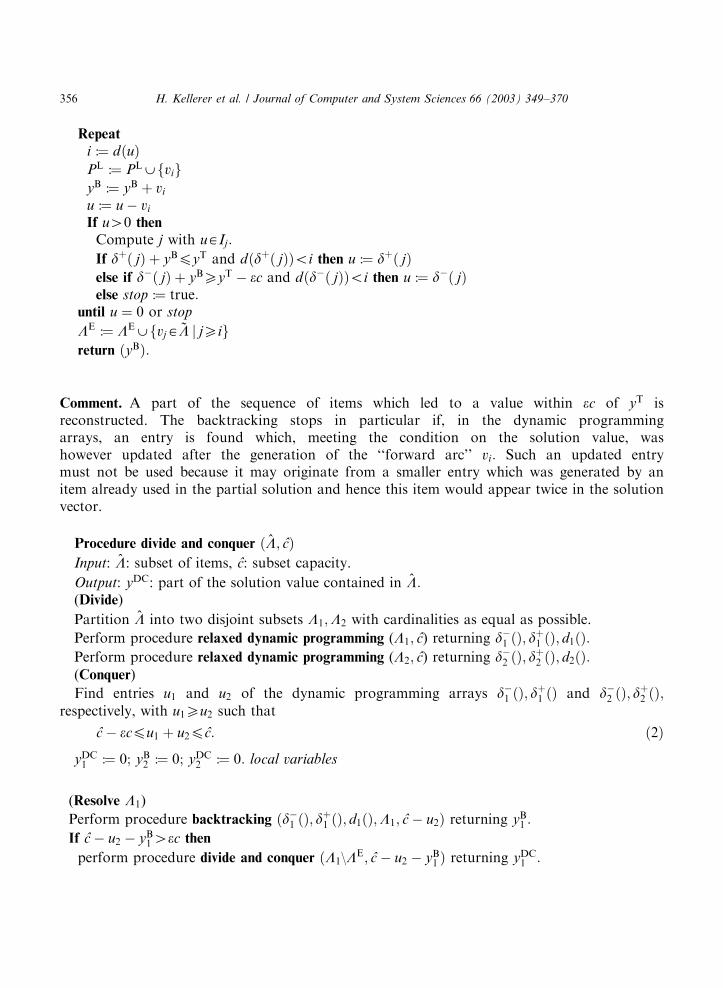
Repeat

i :¼ dðuÞPL :¼ PL,fvigyB :¼ yB þ vi

u :¼ u � vi

If u40 then

Compute j with uAIj:

If dþð jÞ þ yBpyT and dðdþð jÞÞoi then u :¼ dþð jÞelse if d�ð jÞ þ yB

XyT � ec and dðd�ð jÞÞoi then u :¼ d�ð jÞelse stop :¼ true:

until u ¼ 0 or stop

LE :¼ LE,fvjA *L j jXigreturn ðyBÞ:

Comment. A part of the sequence of items which led to a value within ec of yT isreconstructed. The backtracking stops in particular if, in the dynamic programmingarrays, an entry is found which, meeting the condition on the solution value, washowever updated after the generation of the ‘‘forward arc’’ vi: Such an updated entrymust not be used because it may originate from a smaller entry which was generated by anitem already used in the partial solution and hence this item would appear twice in the solutionvector.

Procedure divide and conquer ð #L; cÞInput: #L: subset of items, c: subset capacity.

Output: yDC: part of the solution value contained in #L:(Divide)

Partition #L into two disjoint subsets L1;L2 with cardinalities as equal as possible.

Perform procedure relaxed dynamic programming (L1; c) returning d�1 ðÞ; dþ1 ðÞ; d1ðÞ:Perform procedure relaxed dynamic programming (L2; c) returning d�2 ðÞ; dþ2 ðÞ; d2ðÞ:(Conquer)

Find entries u1 and u2 of the dynamic programming arrays d�1 ðÞ; dþ1 ðÞ and d�2 ðÞ; d

þ2 ðÞ;

respectively, with u1Xu2 such that

c � ecpu1 þ u2pc: ð2Þ

yDC1 :¼ 0; yB2 :¼ 0; yDC

2 :¼ 0: local variables

(Resolve L1)

Perform procedure backtracking ðd�1 ðÞ; dþ1 ðÞ; d1ðÞ;L1; c � u2Þ returning yB1 :

If c � u2 � yB14ec then

perform procedure divide and conquer ðL1\LE; c � u2 � yB1 Þ returning yDC1 :


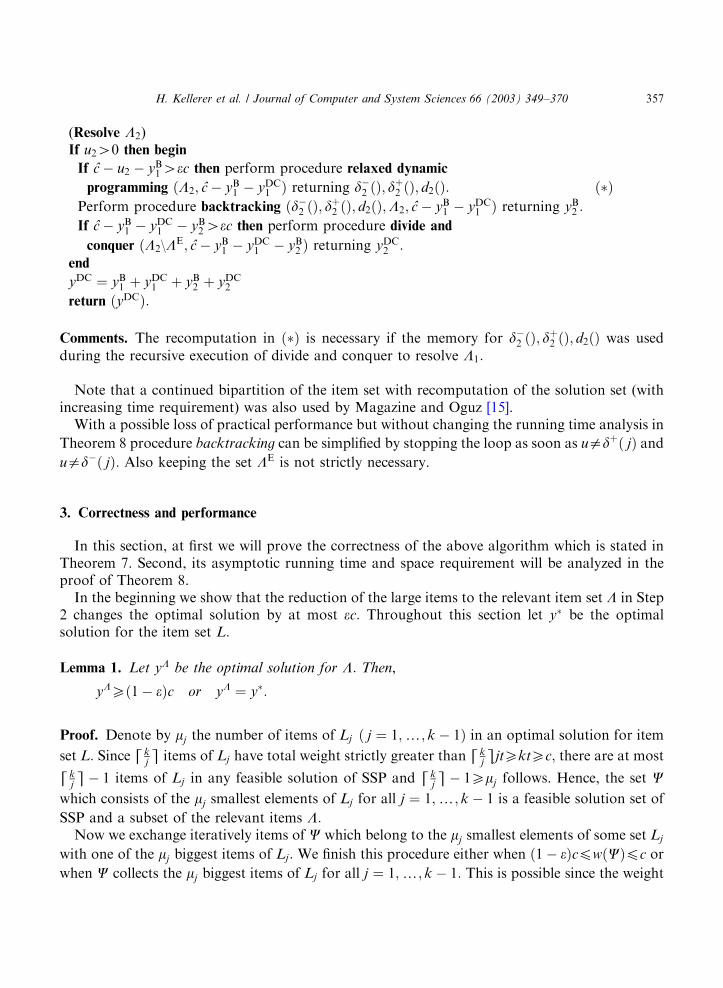
(Resolve L2)If u240 then begin

If c � u2 � yB14ec then perform procedure relaxed dynamic

programming ðL2; c � yB1 � yDC

1 Þ returning d�2 ðÞ; dþ2 ðÞ; d2ðÞ: ð�Þ

Perform procedure backtracking ðd�2 ðÞ; dþ2 ðÞ; d2ðÞ;L2; c � yB1 � yDC1 Þ returning yB2 :

If c � yB1 � yDC1 � yB

24ec then perform procedure divide and

conquer ðL2\LE; c � yB1 � yDC1 � yB

2 Þ returning yDC2 :

end

yDC ¼ yB1 þ yDC1 þ yB

2 þ yDC2

return ðyDCÞ:

Comments. The recomputation in ð�Þ is necessary if the memory for d�2 ðÞ; dþ2 ðÞ; d2ðÞ was usedduring the recursive execution of divide and conquer to resolve L1:

Note that a continued bipartition of the item set with recomputation of the solution set (withincreasing time requirement) was also used by Magazine and Oguz [15].With a possible loss of practical performance but without changing the running time analysis in

Theorem 8 procedure backtracking can be simplified by stopping the loop as soon as uadþð jÞ anduad�ð jÞ: Also keeping the set LE is not strictly necessary.

3. Correctness and performance

In this section, at first we will prove the correctness of the above algorithm which is stated inTheorem 7. Second, its asymptotic running time and space requirement will be analyzed in theproof of Theorem 8.In the beginning we show that the reduction of the large items to the relevant item set L in Step

2 changes the optimal solution by at most ec: Throughout this section let y� be the optimalsolution for the item set L:

Lemma 1. Let yL be the optimal solution for L: Then,

yLXð1� eÞc or yL ¼ y�:

Proof. Denote by mj the number of items of Lj ð j ¼ 1;y; k � 1Þ in an optimal solution for item

set L: Since Jkjn items of Lj have total weight strictly greater than Jk

jnjtXktXc; there are at most

Jkjn� 1 items of Lj in any feasible solution of SSP and Jk

jn� 1Xmj follows. Hence, the set C

which consists of the mj smallest elements of Lj for all j ¼ 1;y; k � 1 is a feasible solution set of

SSP and a subset of the relevant items L:Now we exchange iteratively items of C which belong to the mj smallest elements of some set Lj

with one of the mj biggest items of Lj: We finish this procedure either when ð1� eÞcpwðCÞpc or

when C collects the mj biggest items of Lj for all j ¼ 1;y; k � 1: This is possible since the weight


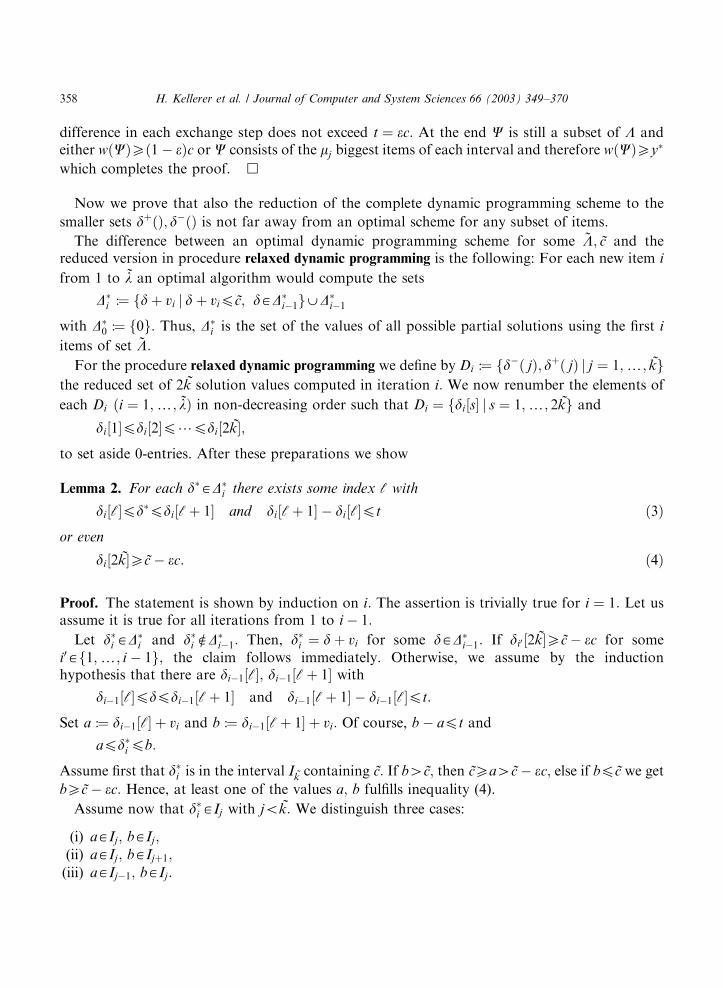
difference in each exchange step does not exceed t ¼ ec: At the end C is still a subset of L andeither wðCÞXð1� eÞc orC consists of the mj biggest items of each interval and therefore wðCÞXy�

which completes the proof. &

Now we prove that also the reduction of the complete dynamic programming scheme to the

smaller sets dþðÞ; d�ðÞ is not far away from an optimal scheme for any subset of items.

The difference between an optimal dynamic programming scheme for some *L; c and thereduced version in procedure relaxed dynamic programming is the following: For each new item i

from 1 to *l an optimal algorithm would compute the sets

D�i :¼ fdþ vi j dþ vipc; dAD�

i�1g,D�i�1

with D�0 :¼ f0g: Thus, D�

i is the set of the values of all possible partial solutions using the first i

items of set *L:For the procedure relaxed dynamic programming we define by Di :¼ fd�ð jÞ; dþð jÞ j j ¼ 1;y; kg

the reduced set of 2k solution values computed in iteration i: We now renumber the elements of

each Di ði ¼ 1;y; *lÞ in non-decreasing order such that Di ¼ fdi½s j s ¼ 1;y; 2kg and

di½1pdi½2p?pdi½2k;to set aside 0-entries. After these preparations we show

Lemma 2. For each d�AD�i there exists some index c with

di½cpd�pdi½cþ 1 and di½cþ 1 � di½cpt ð3Þor even

di½2kXc � ec: ð4Þ

Proof. The statement is shown by induction on i: The assertion is trivially true for i ¼ 1: Let usassume it is true for all iterations from 1 to i � 1:

Let d�i AD�i and d�i eD�

i�1: Then, d�i ¼ dþ vi for some dAD�i�1: If di0 ½2kXc � ec for some

i0Af1;y; i � 1g; the claim follows immediately. Otherwise, we assume by the inductionhypothesis that there are di�1½c; di�1½cþ 1 with

di�1½cpdpdi�1½cþ 1 and di�1½cþ 1 � di�1½cpt:

Set a :¼ di�1½c þ vi and b :¼ di�1½cþ 1 þ vi: Of course, b � apt and

apd�i pb:

Assume first that d�i is in the interval Ik containing c: If b4c; then cXa4c � ec; else if bpc we get

bXc � ec: Hence, at least one of the values a; b fulfills inequality (4).

Assume now that d�i AIj with jok: We distinguish three cases:

(i) aAIj; bAIj;(ii) aAIj; bAIjþ1;(iii) aAIj�1; bAIj:


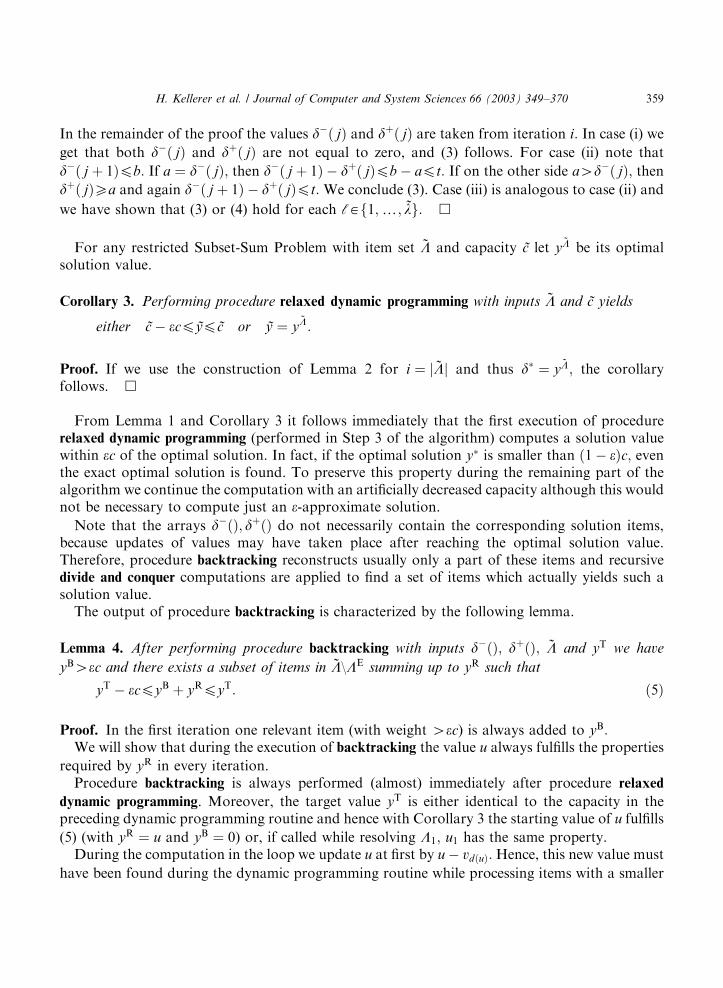
In the remainder of the proof the values d�ð jÞ and dþð jÞ are taken from iteration i: In case (i) we

get that both d�ð jÞ and dþð jÞ are not equal to zero, and (3) follows. For case (ii) note that

d�ð j þ 1Þpb: If a ¼ d�ð jÞ; then d�ð j þ 1Þ � dþð jÞpb � apt: If on the other side a4d�ð jÞ; thendþð jÞXa and again d�ð j þ 1Þ � dþð jÞpt: We conclude (3). Case (iii) is analogous to case (ii) and

we have shown that (3) or (4) hold for each cAf1;y; *lg: &

For any restricted Subset-Sum Problem with item set *L and capacity c let y*L be its optimal

solution value.

Corollary 3. Performing procedure relaxed dynamic programming with inputs *L and c yields

either c � ecpypc or y ¼ y*L:

Proof. If we use the construction of Lemma 2 for i ¼ j *Lj and thus d� ¼ y*L; the corollary

follows. &

From Lemma 1 and Corollary 3 it follows immediately that the first execution of procedurerelaxed dynamic programming (performed in Step 3 of the algorithm) computes a solution valuewithin ec of the optimal solution. In fact, if the optimal solution y� is smaller than ð1� eÞc; eventhe exact optimal solution is found. To preserve this property during the remaining part of thealgorithm we continue the computation with an artificially decreased capacity although this wouldnot be necessary to compute just an e-approximate solution.

Note that the arrays d�ðÞ; dþðÞ do not necessarily contain the corresponding solution items,because updates of values may have taken place after reaching the optimal solution value.Therefore, procedure backtracking reconstructs usually only a part of these items and recursivedivide and conquer computations are applied to find a set of items which actually yields such asolution value.The output of procedure backtracking is characterized by the following lemma.

Lemma 4. After performing procedure backtracking with inputs d�ðÞ; dþðÞ; *L and yT we have

yB4ec and there exists a subset of items in *L\LE summing up to yR such that

yT � ecpyB þ yRpyT: ð5Þ

Proof. In the first iteration one relevant item (with weight 4ec) is always added to yB:We will show that during the execution of backtracking the value u always fulfills the properties

required by yR in every iteration.Procedure backtracking is always performed (almost) immediately after procedure relaxed

dynamic programming. Moreover, the target value yT is either identical to the capacity in thepreceding dynamic programming routine and hence with Corollary 3 the starting value of u fulfills

(5) (with yR ¼ u and yB ¼ 0) or, if called while resolving L1; u1 has the same property.During the computation in the loop we update u at first by u � vdðuÞ:Hence, this new value must

have been found during the dynamic programming routine while processing items with a smaller


index than that leading to the old u: Therefore, we get for u40; that d�ð jÞpupdþð jÞ: At this

point yT � ecpyB þ vdðuÞ þ u � vdðuÞpyT still holds. Then there are two possible updates of u: We

may set u :¼ dþð jÞ thus not decreasing u and still fulfilling (5). We may also have u :¼ d�ð jÞ withthe condition that d�ð jÞXyT � yB � ec and hence inequality (5) still holds because u was less than

yT � yB and is further decreased.

Ending the loop in backtracking there is either u ¼ 0; and (5) is fulfilled with yR ¼ 0; or stop ¼true, and by the above argument yR :¼ u yields the required properties.At the end of each iteration (except possibly the last one) u is always set to an entry in the

dynamic programming array which was reached by an item with index smaller than the item

previously put into PL: Naturally, all items leading to this entry must have had even smaller

indices. Therefore, the final value yR must be a combination of items with indices less than that of

the last item added to PL; i.e. from the set *L\LE: &

In the following, we show that the divide and conquer recursions actually generate a suitablesolution for the given capacity.

Lemma 5. If at the start of procedure divide and conquer there exists a subset of #L with weight y

such that

c � ecpypc;

then there exist u1; u2 fulfilling (2).

Proof. Obviously, we can write y ¼ y1 þ y2 with y1 being the sum of items from L1 and y2 fromL2: If y1 or y2 is 0; the result follows immediately from Lemma 2 setting u1 or u2 equal to 0,respectively.With Lemma 2 we conclude that after the Divide step there exist values a1; b1 from the dynamic

programming arrays d�1 ðÞ; dþ1 ðÞ witha1py1pb1 and b1 � a1pt:

Analogously, there exist a2; b2 from d�2 ðÞ; dþ2 ðÞ witha2py2pb2 and b2 � a2pt:

Now it is easy to see that at least one of the four pairs from fa1; b1g � fa2; b2g fulfills (2). &

The return value of the procedure divide and conquer can be characterized in thefollowing way.

Lemma 6. If, performing procedure divide and conquer with inputs #L and c;

there exists a subset of #L with weight y such that c � ecpypc; ð6Þ

then also the returned value yDC fulfills

c � ecpyDCpc:


Proof. Lemma 5 guarantees that under condition (6) there are always values u1; u2 satisfying (2).The recursive structure of the divide and conquer calls can be seen as an ordered, not necessarily

complete, binary rooted tree. Each node in the tree corresponds to one call of divide and conquer

with the root indicating the first call from Step 3. Furthermore, every node may have up to twochild nodes, the left child corresponding to a call of divide and conquer to resolve L1 and the right

child corresponding to a call generated while resolving L2: As the left child is always visited first (ifit exists), the recursive structure corresponds to a preordered tree walk.In the following, we will show the statement of the lemma by backwards induction moving

‘‘upwards’’ in the tree, i.e. beginning with its leaves and applying induction to the inner nodes.We start with the leaves of the tree, i.e. executions of divide and conquer with no further

recursive calls. Therefore, we have yDC1 ¼ 0 after resolving L1 and by considering the condition for

not calling the recursion

c � u2 � ecpyB1pc � u2:

Resolving L2 we either have u2 ¼ 0 and hence yDC ¼ yB1 and we are done with the previous

inequality or we get

c � yB1 � ecpyB

2pc � yB1

and hence with yDC2 ¼ 0

c � ecpyB1 þ yB

2 ¼ yDCpc:

For all other nodes we show that the above implication is true for an arbitrary node under theinductive assumption that it is true for all its children. To do so, we will prove that if condition (6)holds, it is also fulfilled for any child of the node and hence by induction the child nodes returnvalues according to the above implication. These values will be used to show that also the current

node returns the desired yDC:If the node under consideration has a left child, we know by Lemma 4 that after performing

procedure backtracking with yT ¼ c � u2; there exists yR1 fulfilling

c � yB1 � u2 � ecpyR1 pc � yB1 � u2

which is equivalent to the required condition (6) for the left child node. By induction, we get withthe above statement for the return value of the left child (after rearranging)

c � u2 � ecpyB1 þ yDC1 pc � u2:

If there is no left child (i.e. for the case that yDC1 ¼ 0), we get from the condition for this event

c � u2 � ecpyB1pc � u2:

If u2 ¼ 0 and hence yDC ¼ yB1 þ yDC1 ; we are done immediately in both of these two cases.

If there is a right child node we proceed along the same lines. From Lemma 4 we know that

after performing backtracking with yT ¼ c � yB1 � yDC

1 while resolving L2 there exists yR2 with

c � yB1 � yDC

1 � yB2 � ecpyR2 pc � yB1 � yDC

1 � yB2 ;

which is precisely condition (6) for the right child node.


Hence, by induction we can apply the above implication on the right child and get

c � yB1 � yDC

1 � yB2 � ecpyDC2 pc � yB1 � yDC

1 � yB2

which is (after rearranging) equivalent to the desired statement for yDC in the currentnode.

If there is no right child (i.e. yDC2 ¼ 0), the result follows from the corresponding condition. &

Applying this lemma to the beginning of the recursion and considering also the small items wecan finally state

Theorem 7. Algorithm ðAÞ is an ð1� eÞ-approximation algorithm for the Subset-Sum Problem. Inparticular,

zAXð1� eÞc or zA ¼ z�:

Moreover, the bound is tight.

Proof. As shown in Lemma 1 the reduction of the total item set to L in Step 2 does not eliminateall e-approximate solutions. Hence, it is sufficient to show the claim for the set of relevant items,namely that at the end of Step 3 we have either

yLXð1� eÞc or yL ¼ yL:

If the first execution of relaxed dynamic programming in Step 3 returns yoð1� eÞc we know fromCorollary 3 that we have found the optimum solution value over the set of relevant items.

Continuing with the updated capacity c the claim yL ¼ yL would follow immediately from the firstalternative for the new capacity. Therefore, we will assume in the sequel that in Step 3 we find

yXð1� eÞc and only prove that yLXð1� eÞc:

If divide and conquer is not performed at all this relation follows immediately.

It remains to be shown that for yDC; i.e. the return value of the first execution of divide

and conquer, ð1� eÞc � yBpyDCpc � yB holds, because at the end of Step 3 we set yL :¼yB þ yDC: However, due to Lemma 4 the existence of a value yR satisfying this relation is

established. But this is exactly the condition required in Lemma 6 to guarantee that yDC fulfills theabove.In Step 4 there are only two possibilities: Either there is a small item which is not chosen by the

greedy-type algorithm. But this can only happen if the current solution is already greater thanð1� eÞc and we are done.

In the second case we have SCXA which yields, depending on the outcome of Step 3,

either zA ¼ yL þ wðSÞXð1� eÞc þ wðSÞXð1� eÞcor zA ¼ yL þ wðSÞ ¼ yL þ wðSÞ ¼ y� þ wðSÞXz� ) zA ¼ z�

by Lemma 1.To prove that the bound is tight, we consider the following series of instances: e ¼ 1=k; n ¼

2k � 1; c ¼ kR with R4k � 1 and w1 ¼ ? ¼ wk�1 ¼ R þ 1; wk ¼ ? ¼ w2k�1 ¼ R: It follows


that zA ¼ ðk � 1ÞR þ ðk � 1Þ and z� ¼ kR: The performance ratio tends to ðk � 1Þ=k when Rtends to infinity. &

The asymptotic running time of algorithm (A) is analyzed in the following theorem.

Theorem 8. For every accuracy e40 ð0oeo1Þ algorithm ðAÞ runs in time Oðminfn � 1=e; n þ1=e2 logð1=eÞgÞ and space Oðn þ 1=eÞ: Especially, only Oð1=eÞ storage locations are needed inaddition to the description of the input itself.

Proof. Recall that k is in Oð1=eÞ and t ¼ ec: Throughout the algorithm, the relevant spacerequirement consists of storing the n items and six dynamic programming arrays

d�1 ðÞ; dþ1 ðÞ; d1ðÞ; d�2 ðÞ; dþ2 ðÞ and d2ðÞ with length k:Special attention has to be paid to the implicit memory necessary for the recursion of procedure

divide and conquer. To avoid using new memory for the dynamic programming array in everyrecursive call, we always use the same space for the six arrays. But this means that after returning

from a recursive call while resolving L1 the previous data in d�2 and dþ2 is lost and has to be

recomputed.

A natural bipartition of each #L can be achieved by taking the first half and second half of thegiven sequence of items. This means that each subset Li can be represented by the first and the lastindex of consecutively following items from the ground set. If for some reason a different partitionscheme is desired, a labeling method can be used to associate a unique number with each call of

divide and conquer and with all items belonging to the corresponding set #L:Therefore, each call to divide and conquer requires only a constant amount of memory and the

recursion depth is bounded by Oðlog kÞ: Hence, all computations can be performed within Oðn þ1=eÞ space.Step 1 requires Oðn þ kÞ time. Selecting the Jk

jn� 1 items with smallest and largest weight for

Lj (j ¼ 1;y; k � 1) in Step 2 can be done efficiently as described in [3] and takes altogether

Oðn þ kÞ time. The total number l of relevant items of L is bounded from above by lpn and by

lp2Xk�1

j¼1

k

j

� �� 1

� �p2k

Xk�1

j¼1

1

jo2k log k: ð7Þ

Consequently, l is of order Oðminfn; 1=e logð1=eÞgÞ:Each call of procedure dynamic programming with parameters *L and c (let *l :¼ j *Lj) takes

Oð*l � c=tÞ time, as for each item i; i ¼ 1;y; *l; we have to consider only jDij candidates forupdating the dynamic programming arrays, a number which is clearly in Oðc=tÞ:Procedure backtracking always immediately follows procedure relaxed dynamic programming

and can clearly be done in OðyT=tÞ time with yTpc:

Therefore, applying the above bound on l Step 3 requires Oðminfn; k log kgc=tÞ; i.e. Oðminfn �1=e; 1=e2 logð1=eÞgÞ time plus the effort of the divide and conquer execution which will be treatedbelow. Clearly, Step 4 requires OðnÞ time.To estimate the running time of the recursive procedure divide and conquer we recall the

representation of the recursion as a binary tree as used in the proof of Lemma 6. A node is said to


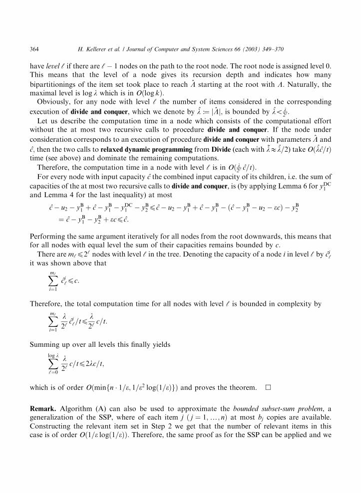
have level c if there are c� 1 nodes on the path to the root node. The root node is assigned level 0.This means that the level of a node gives its recursion depth and indicates how many

bipartitionings of the item set took place to reach #L starting at the root with L: Naturally, themaximal level is log l which is in Oðlog kÞ:Obviously, for any node with level c the number of items considered in the corresponding

execution of divide and conquer, which we denote by #l :¼ j #Lj; is bounded by #lo l2c:

Let us describe the computation time in a node which consists of the computational effortwithout the at most two recursive calls to procedure divide and conquer. If the node under

consideration corresponds to an execution of procedure divide and conquer with parameters #L and

c; then the two calls to relaxed dynamic programming from Divide (each with *lE#l=2) take Oð#lc=tÞtime (see above) and dominate the remaining computations.

Therefore, the computation time in a node with level c is in Oð l2c

c=tÞ:For every node with input capacity c the combined input capacity of its children, i.e. the sum of

capacities of the at most two recursive calls to divide and conquer, is (by applying Lemma 6 for yDC1

and Lemma 4 for the last inequality) at most

c � u2 � yB1 þ c � yB

1 � yDC1 � yB2pc � u2 � yB

1 þ c � yB1 � ðc � yB

1 � u2 � ecÞ � yB2

¼ c � yB1 � yB

2 þ ecpc:

Performing the same argument iteratively for all nodes from the root downwards, this means thatfor all nodes with equal level the sum of their capacities remains bounded by c:

There are mcp2c nodes with level c in the tree. Denoting the capacity of a node i in level c by cic

it was shown above thatXmc

i¼1

cicpc:

Therefore, the total computation time for all nodes with level c is bounded in complexity byXmc

i¼1

l2c

cic=tp

l2c

c=t:

Summing up over all levels this finally yields

Xlog l

c¼0

l2c

c=tp2lc=t;

which is of order Oðminfn � 1=e; 1=e2 logð1=eÞgÞ and proves the theorem. &

Remark. Algorithm (A) can also be used to approximate the bounded subset-sum problem, ageneralization of the SSP, where of each item j ð j ¼ 1;y; nÞ at most bj copies are available.

Constructing the relevant item set in Step 2 we get that the number of relevant items in thiscase is of order Oð1=e logð1=eÞÞ: Therefore, the same proof as for the SSP can be applied and we


obtain an approximation scheme with running time Oðn þ 1=e2 logð1=eÞÞ and space requirementOðn þ 1=eÞ:

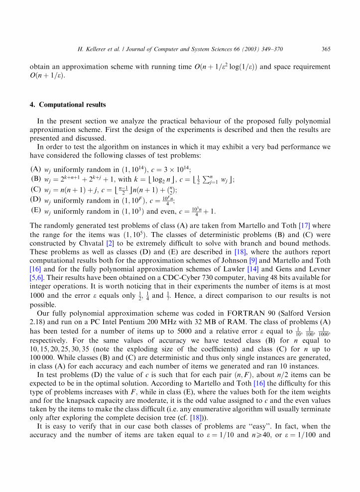
4. Computational results

In the present section we analyze the practical behaviour of the proposed fully polynomialapproximation scheme. First the design of the experiments is described and then the results arepresented and discussed.In order to test the algorithm on instances in which it may exhibit a very bad performance we

have considered the following classes of test problems:

(A) wj uniformly random in ð1; 1014Þ; c ¼ 3� 1014;(B) wj ¼ 2kþnþ1 þ 2kþj þ 1; with k ¼ Ilog2 nm; c ¼ I1

2

Pnj¼1 wjm;

(C) wj ¼ nðn þ 1Þ þ j; c ¼ In�12mnðn þ 1Þ þ ðn

2Þ;

(D) wj uniformly random in ð1; 10F Þ; c ¼ 10F n4;

(E) wj uniformly random in ð1; 103Þ and even, c ¼ 103n4

þ 1:

The randomly generated test problems of class (A) are taken from Martello and Toth [17] where

the range for the items was ð1; 105Þ: The classes of deterministic problems (B) and (C) wereconstructed by Chvatal [2] to be extremely difficult to solve with branch and bound methods.These problems as well as classes (D) and (E) are described in [18], where the authors reportcomputational results both for the approximation schemes of Johnson [9] and Martello and Toth[16] and for the fully polynomial approximation schemes of Lawler [14] and Gens and Levner[5,6]. Their results have been obtained on a CDC-Cyber 730 computer, having 48 bits available forinteger operations. It is worth noticing that in their experiments the number of items is at most

1000 and the error e equals only 12; 14and 1

7: Hence, a direct comparison to our results is not

possible.Our fully polynomial approximation scheme was coded in FORTRAN 90 (Salford Version

2.18) and run on a PC Intel Pentium 200 MHz with 32 MB of RAM. The class of problems (A)

has been tested for a number of items up to 5000 and a relative error e equal to 110; 1100

; 11000

;

respectively. For the same values of accuracy we have tested class (B) for n equal to10; 15; 20; 25; 30; 35 (note the exploding size of the coefficients) and class (C) for n up to100 000: While classes (B) and (C) are deterministic and thus only single instances are generated,in class (A) for each accuracy and each number of items we generated and ran 10 instances.In test problems (D) the value of c is such that for each pair ðn;FÞ; about n=2 items can be

expected to be in the optimal solution. According to Martello and Toth [16] the difficulty for thistype of problems increases with F ; while in class (E), where the values both for the item weightsand for the knapsack capacity are moderate, it is the odd value assigned to c and the even valuestaken by the items to make the class difficult (i.e. any enumerative algorithm will usually terminateonly after exploring the complete decision tree (cf. [18])).It is easy to verify that in our case both classes of problems are ‘‘easy’’. In fact, when the

accuracy and the number of items are taken equal to e ¼ 1=10 and nX40; or e ¼ 1=100 and


nX400; or e ¼ 1=1000 and nX4000; respectively, all the items are small items so that theguaranteed bounds on the worst-case performance are easily obtained through Step 4 of thealgorithm (i.e. by only applying the greedy-type algorithm). For this reason the results for thesetwo classes are not reported. We only notice that, e.g. for F ¼ 6; the errors and the running timesfound for each pair ðn; eÞ in the two classes are very similar even if in the instances of class (E) thealgorithm finds the optimal solution more often than in those of class (D).Now we analyze classes (A)–(C) discussing their results separately. The errors were determined

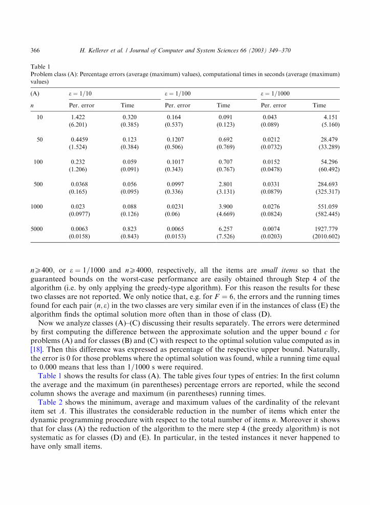
by first computing the difference between the approximate solution and the upper bound c forproblems (A) and for classes (B) and (C) with respect to the optimal solution value computed as in[18]. Then this difference was expressed as percentage of the respective upper bound. Naturally,the error is 0 for those problems where the optimal solution was found, while a running time equalto 0.000 means that less than 1=1000 s were required.Table 1 shows the results for class (A). The table gives four types of entries: In the first column

the average and the maximum (in parentheses) percentage errors are reported, while the secondcolumn shows the average and maximum (in parentheses) running times.Table 2 shows the minimum, average and maximum values of the cardinality of the relevant

item set L: This illustrates the considerable reduction in the number of items which enter thedynamic programming procedure with respect to the total number of items n: Moreover it showsthat for class (A) the reduction of the algorithm to the mere step 4 (the greedy algorithm) is notsystematic as for classes (D) and (E). In particular, in the tested instances it never happened tohave only small items.

Table 1

Problem class (A): Percentage errors (average (maximum) values), computational times in seconds (average (maximum)

values)

(A) e ¼ 1=10 e ¼ 1=100 e ¼ 1=1000

n Per. error Time Per. error Time Per. error Time

10 1.422 0.320 0.164 0.091 0.043 4.151

(6.201) (0.385) (0.537) (0.123) (0.089) (5.160)

50 0.4459 0.123 0.1207 0.692 0.0212 28.479

(1.524) (0.384) (0.506) (0.769) (0.0732) (33.289)

100 0.232 0.059 0.1017 0.707 0.0152 54.296

(1.206) (0.091) (0.343) (0.767) (0.0478) (60.492)

500 0.0368 0.056 0.0997 2.801 0.0331 284.693

(0.165) (0.095) (0.336) (3.131) (0.0879) (325.317)

1000 0.023 0.088 0.0231 3.900 0.0276 551.059

(0.0977) (0.126) (0.06) (4.669) (0.0824) (582.445)

5000 0.0063 0.823 0.0065 6.257 0.0074 1927.779

(0.0158) (0.843) (0.0153) (7.526) (0.0203) (2010.602)


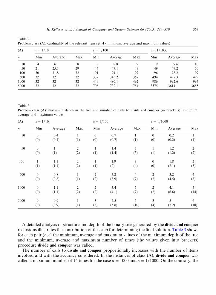
A detailed analysis of structure and depth of the binary tree generated by the divide and conquer

recursions illustrates the contribution of this step for determining the final solution. Table 3 showsfor each pair ðn; eÞ the minimum, average and maximum values of the maximum depth of the treeand the minimum, average and maximum number of times (the values given into brackets)procedure divide and conquer was called.The number of calls to divide and conquer proportionally increases with the number of items

involved and with the accuracy considered. In the instances of class (A), divide and conquer wascalled a maximum number of 14 times for the case n ¼ 1000 and e ¼ 1=1000: On the contrary, the

Table 2

Problem class (A): cardinality of the relevant item set L (minimum, average and maximum values)

(A) e ¼ 1=10 e ¼ 1=100 e ¼ 1=1000

n Min Average Max Min Average Max Min Average Max

10 4 6 8 8 8.8 9 9 9.6 10

50 21 25.1 29 44 47.1 49 49 49.2 50

100 30 31.8 32 91 94.1 97 96 98.2 99

500 32 32 32 337 345.2 357 494 497.3 499

1000 32 32 32 449 480.1 492 986 992.6 997

5000 32 32 32 706 732.1 754 3575 3614 3685

Table 3

Problem class (A): maximum depth in the tree and number of calls to divide and conquer (in brackets), minimum,

average and maximum values

(A) e ¼ 1=10 e ¼ 1=100 e ¼ 1=1000

n Min Average Max Min Average Max Min Average Max

10 0 0.4 1 0 0.7 1 0 0.2 1

(0) (0.4) (1) (0) (0.7) (1) (0) (0.2) (1)

50 0 1 2 1 1.4 3 1 1.2 2

(0) (1) (2) (1) (1.4) (3) (1) (1.2) (2)

100 1 1.1 2 1 1.9 3 0 1.8 2

(1) (1.1) (2) (1) (2) (4) (0) (2.1) (3)

500 0 0.8 1 2 3.2 4 2 3.2 4

(0) (0.8) (1) (2) (3.9) (7) (2) (4.5) (8)

1000 0 1.1 2 2 3.4 5 2 4.1 5

(0) (1.1) (2) (2) (4.1) (7) (2) (6.6) (14)

5000 0 0.9 1 3 4.5 6 3 5 6

(0) (0.9) (1) (3) (5.8) (10) (4) (7.2) (10)


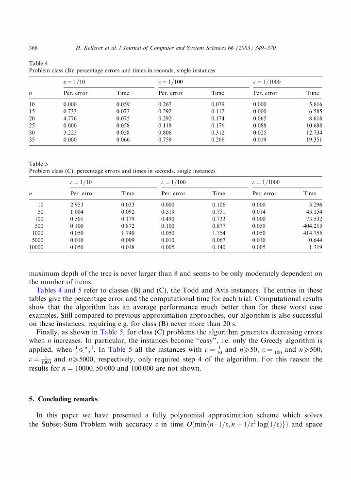
maximum depth of the tree is never larger than 8 and seems to be only moderately dependent onthe number of items.Tables 4 and 5 refer to classes (B) and (C), the Todd and Avis instances. The entries in these

tables give the percentage error and the computational time for each trial. Computational resultsshow that the algorithm has an average performance much better than for these worst caseexamples. Still compared to previous approximation approaches, our algorithm is also successfulon these instances, requiring e.g. for class (B) never more than 20 s:Finally, as shown in Table 5, for class (C) problems the algorithm generates decreasing errors

when n increases. In particular, the instances become ‘‘easy’’, i.e. only the Greedy algorithm is

applied, when 1ep

n�12: In Table 5 all the instances with e ¼ 1

10and nX50; e ¼ 1

100and nX500;

e ¼ 11000

and nX5000; respectively, only required step 4 of the algorithm. For this reason the

results for n ¼ 10000; 50 000 and 100 000 are not shown.

5. Concluding remarks

In this paper we have presented a fully polynomial approximation scheme which solves

the Subset-Sum Problem with accuracy e in time Oðminfn � 1=e; n þ 1=e2 logð1=eÞgÞ and space

Table 4

Problem class (B): percentage errors and times in seconds, single instances

e ¼ 1=10 e ¼ 1=100 e ¼ 1=1000


10 0.000 0.059 0.267 0.079 0.000 5.616

15 0.733 0.073 0.292 0.112 0.000 6.585

20 4.776 0.075 0.292 0.174 0.065 8.618

25 0.000 0.058 0.118 0.176 0.088 10.688

30 3.225 0.058 0.806 0.312 0.025 12.734

35 0.000 0.066 0.759 0.266 0.019 19.351

Table 5

Problem class (C): percentage errors and times in seconds, single instances

e ¼ 1=10 e ¼ 1=100 e ¼ 1=1000


10 2.953 0.033 0.000 0.106 0.000 5.296

50 1.004 0.092 0.519 0.751 0.014 45.154

100 0.501 0.179 0.490 0.733 0.000 73.532

500 0.100 0.872 0.100 0.877 0.050 404.215

1000 0.050 1.740 0.050 1.754 0.050 414.755

5000 0.010 0.009 0.010 0.067 0.010 0.644

10000 0.050 0.018 0.005 0.140 0.005 1.319


Oðn þ 1=eÞ: Moreover, for all instances with subset capacity c where the optimal solution is lessthan ð1� eÞc our algorithm actually computes the optimal solution.With this scheme we could solve large instances efficiently with high accuracy on a personal

computer which were intractable by known approximation algorithms on bigger computers (e.g. aCDC-Cyber 730).An objection against fully polynomial approximation schemes for the SSP was so far that ‘‘they

can be impractical for relatively large values of 1=e’’ [17]. Since for this scheme the memoryrequirement is only Oðn þ 1=eÞ; there should be no reason to prefer polynomial approximationschemes to this fully polynomial approximation scheme.The divide and conquer technique was also used in an improved approximation algorithm for

the knapsack problem (see [11,12]).Finally, an interesting open problem would be to get rid of the logarithm in the time bound for

the algorithm, i.e. to reduce the time complexity to Oðminfn � 1=e; n þ 1=e2gÞ:

References

[1] R.E. Bellman, Dynamic Programming, Princeton University Press, Princeton, 1957.

[2] V. Chvatal, Hard knapsack problems, Oper. Res. 28 (1980) 1402–1411.

[3] D. Dor, U. Zwick, Selecting the median, in: Proceedings of the Sixth ACM-SIAM Symposium on Discrete

Algorithms, 1995, pp. 28–35.

[4] M.R. Garey, D.S. Johnson, Computers and Intractability: A Guide to the Theory of NP-Completeness, Freeman,

San Francisco, 1979.

[5] G.V. Gens, E.V. Levner, Approximation algorithms for certain universal problems in scheduling theory, Soviet J.

Comput. System Sci. 6 (1978) 31–36.

[6] G.V. Gens, E.V. Levner, Fast approximation algorithms for knapsack type problems, in: K. Iracki, K.

Malinowski, S. Walukiewicz (Eds.), Optimization Techniques, Part 2, Lecture Notes in Control and Information

Sciences, Vol. 74, Springer, Berlin, 1980, pp. 185–194.

[7] G.V. Gens, E.V. Levner, A fast approximation algorithm for the subset-sum problem, INFOR 32 (1994)

143–148.

[8] O.H. Ibarra, C.E. Kim, Fast approximation algorithms for the knapsack and sum of subset problems, J. ACM 22

(1975) 463–468.

[9] D.S. Johnson, Approximation algorithms for combinatorial problems, J. Comput. System Sci. 9 (1974)

339–356.

[10] R.M. Karp, The fast approximate solution of hard combinatorial problems, Proceedings of the Sixth Southeastern

Conference on Combinatorics, Graph Theory, and Computing, Utilitas Mathematica Publishing, Winnipeg, 1975,

pp. 15–31.

[11] H. Kellerer, U. Pferschy, A new fully polynomial time approximation scheme for the knapsack problem,

J. Combin. Optim. 3 (1999) 59–71.

[12] H. Kellerer, U. Pferschy, Improved dynamic programming in connection with an FPTAS for the knapsack

problem, J. Combin. Optim., to appear.

[13] H. Kellerer, U. Pferschy, M.G. Speranza, An efficient fully polynomial approximation scheme for the subset-sum

problem, Proceedings of the Eighth ISAAC Symposium, Springer Lecture Notes in Computer Science, Vol. 1350,

Springer, Berlin, 1997, pp. 394–403.

[14] E. Lawler, Fast approximation algorithms for knapsack problems, Math. Oper. Res. 4 (1979) 339–356.

[15] M.J. Magazine, O. Oguz, A fully polynomial approximation algorithm for the 0–1 knapsack problem, European

J. Oper. Res. 8 (1981) 270–273.

[16] S. Martello, P. Toth, Worst-case analysis of greedy algorithms for the subset-sum problem, Math. Programming

28 (1984) 198–205.


[17] S. Martello, P. Toth, Approximation schemes for the subset-sum problem: survey and experimental results,

European J. Oper. Res. 22 (1985) 56–69.

[18] S. Martello, P. Toth, Knapsack Problems: Algorithms and Computer Implementations, Wiley, Chichester,

1990.

[19] D. Pisinger, Linear time algorithms for knapsack problems with bounded weight, J. Algorithms 33 (1999)

1–14.


Documents

An efficient fully polynomial approximation scheme for the Subset-Sum Problem