Embed Size (px)
Citation preview

VILNIUS GEDIMINAS TECHNICAL UNIVERSITY
Tomyslav SLEDEVIČ
AN EFFICIENT IMPLEMENTATION OFLATTICE-LADDER MULTILAYERPERCEPTRONS IN FIELDPROGRAMMABLE GATE ARRAYS
DOCTORAL DISSERTATION
TECHNOLOGICAL SCIENCES,ELECTRICAL AND ELECTRONIC ENGINEERING (01T)
Vilnius 2016

Doctoral dissertation was prepared at Vilnius Gediminas Technical University in2012–2016.
Scientific supervisor
Prof. Dr Dalius NAVAKAUSKAS (Vilnius Gediminas Technical University,Electrical and Electronic Engineering – 01T).
The Dissertation Defense Council of Scientific Field of Electrical and ElectronicEngineering of Vilnius Gediminas Technical University:
Chairman
Prof. Dr Vytautas URBANAVIČIUS (Vilnius Gediminas Technical University,Electrical and Electronic Engineering – 01T).
Members:
Prof. Dr Habil Arūnas LUKOŠEVIČIUS (Kaunas University of Technology,Electrical and Electronic Engineering – 01T),Prof. Dr Jurij NOVICKIJ (Vilnius Gediminas Technical University, Electricaland Electronic Engineering – 01T),Prof. Dr Habil Adolfas Laimutis TELKSNYS (Vilnius University, InformaticsEngineering – 07T),Dr Pawel WAWRZYNSKI (Warsaw University of Technology, Electrical andElectronic Engineering – 01T).
The dissertation will be defended at the public meeting of the DissertationDefense Council of Electrical and Electronic Engineering in the Senate Hall ofVilnius Gediminas Technical University at 2 p. m. on 8 June 2016.
Address: Saulėtekio al. 11, LT-10223 Vilnius, Lithuania.Tel. +370 5 274 4956; fax +370 5 270 0112; e-mail: [email protected]
A notification on the intend defending of the dissertation was send on 6 May2016.A copy of the doctoral dissertation is available for review at VGTU repositoryhttp://dspace.vgtu.lt and at the Library of Vilnius Gediminas TechnicalUniversity (Saulėtekio al. 14, LT-10223 Vilnius, Lithuania).
VGTU leidyklos TECHNIKA 2371-M mokslo literatūros knyga
Parengta LATEX2ε sistema
ISBN 978-609-457-933-2
© VGTU leidykla TECHNIKA, 2016
© TomyslavSledevič, 2016

VILNIAUS GEDIMINO TECHNIKOS UNIVERSITETAS
Tomyslav SLEDEVIČ
PYNUČIŲ-KOPĖTĖLIŲDAUGIASLUOKSNIŲ PERCEPTRONŲEFEKTYVUS ĮGYVENDINIMASLAUKU PROGRAMUOJAMOMISLOGINĖMIS MATRICOMIS
MOKSLO DAKTARO DISERTACIJA
TECHNOLOGIJOS MOKSLAI,ELEKTROS IR ELEKTRONIKOS INŽINERIJA (01T)
Vilnius 2016
Disertacija rengta 2012–2016 metais Vilniaus Gedimino technikos universitete.
Vadovas
prof. dr. Dalius NAVAKAUSKAS (Vilniaus Gedimino technikos universitetas,elektros ir elektronikos inžinerija – 01T).
Vilniaus Gedimino technikos universiteto Elektros ir elektronikos inžinerijosmokslo krypties disertacijos gynimo taryba:
Pirmininkas
prof. dr. Vytautas URBANAVIČIUS (Vilniaus Gedimino technikosuniversitetas, elektros ir elektronikos inžinerija – 01T).
Nariai:
prof. habil. dr. Arūnas LUKOŠEVIČIUS (Kauno technologijos universitetas,elektros ir elektronikos inžinerija – 01T),prof. dr. Jurij NOVICKIJ (Vilniaus Gedimino technikos universitetas, elektrosir elektronikos inžinerija – 01T),prof. habil. dr. Adolfas Laimutis TELKSNYS (Vilniaus universitetas,informatikos inžinerija – 07T),dr. Pawel WAWRZYNSKI (Varšuvos technologijos universitetas, elektros irelektronikos inžinerija – 01T).
Disertacija bus ginama viešame Elektros ir elektronikos inžinerijos mokslokrypties disertacijos gynimo tarybos posėdyje 2016 m. birželio 8 d. 14 val.
Vilniaus Gedimino technikos universiteto senato posėdžių salėje.
Adresas: Saulėtekio al. 11, LT-10223 Vilnius, Lietuva.Tel. +370 5 274 4956; fax +370 5 270 0112; el. paštas: [email protected]
Pranešimai apie numatomą ginti disertaciją išsiųsti 2016 m. gegužės 6 d..
Disertaciją galima peržiūrėti VGTU talpykloje http://dspace.vgtu.lt irVilniaus Gedimino technikos universiteto bibliotekoje (Saulėtekio al. 14,LT-10223 Vilnius, Lietuva).

Abstract
The implementation efficiency of electronic systems is a combination of con-flicting requirements, as increasing volumes of computations, accelerating theexchange of data, at the same time increasing energy consumption forcing theresearchers not only to optimize the algorithm, but also to quickly implementin a specialized hardware. Therefore in this work, the problem of efficient andstraightforward implementation of operating in a real-time electronic intelli-gent systems on field-programmable gate array (FPGA) is tackled. The objectof research is specialized FPGA intellectual property (IP) cores that operate ina real-time. In the thesis the following main aspects of the research object areinvestigated: implementation criteria and techniques.
The aim of the thesis is to optimize the FPGA implementation processof selected class dynamic artificial neural networks. In order to solve statedproblem and reach the goal following main tasks of the thesis are formu-lated: rationalize the selection of a class of Lattice-Ladder Multi-Layer Per-ceptron (LLMLP) and its electronic intelligent system test-bed – a speakerdependent Lithuanian speech recognizer, to be created and investigated; de-velop dedicated technique for implementation of LLMLP class on FPGA thatis based on specialized efficiency criteria for a circuitry synthesis; developand experimentally affirm the efficiency of optimized FPGA IP cores used inLithuanian speech recognizer.
The dissertation contains: introduction, four chapters and general conclu-sions. The first chapter reveals the fundamental knowledge on computer-aided-design, artificial neural networks and speech recognition implementation onFPGA. In the second chapter the efficiency criteria and technique of LLMLPIP cores implementation are proposed in order to make multi-objective op-timization of throughput, LLMLP complexity and resource utilization. Thedata flow graphs are applied for optimization of LLMLP computations. Theoptimized neuron processing element is proposed. The IP cores for featuresextraction and comparison are developed for Lithuanian speech recognizer andanalyzed in third chapter. The fourth chapter is devoted for experimental veri-fication of developed numerous LLMLP IP cores. The experiments of isolatedword recognition accuracy and speed for different speakers, signal to noise ra-tios, features extraction and accelerated comparison methods were performed.
The main results of the thesis were published in 12 scientific publications:eight of them were printed in peer-reviewed scientific journals, four of themin a Thomson Reuters Web of Science database, four articles – in conferenceproceedings. The results were presented in 17 scientific conferences.
v

Reziumė
Elektroninių sistemų įgyvendinimo efektyvumas yra prieštaringų reikalavimųderinys, nes didėjančios skaičiavimų apimtys, spartėjantys duomenų mainai,o tuo pačiu didėjantis energijos suvartojimas verčia ne tik optimizuoti algorit-mus, bet ir juos greitai įgyvendinti specializuotoje aparatūroje. Todėl diserta-cijoje sprendžiama realiuoju laiku veikiančių elektroninių intelektualiųjų sis-temų efektyvaus įgyvendinimo lauku programuojama logine matrica (LPLM)problema. Tyrimo objektas yra specializuoti LPLM intelektinės nuosavybės(IN) moduliai veikiantys realiuoju laiku. Disertacijoje tiriami šie, su tiria-muoju objektu susiję, dalykai: įgyvendinimo kriterijai ir metodas.
Disertacijos tikslas – optimizuoti pasirinktos dinaminių dirbtinių neuronųtinklo klasės įgyvendinimo procesą LPLM. Siekiant išspręsti nurodytą prob-lemą ir pasiekti tikslą suformuluojami šie pagrindiniai disertacijoje sprendžia-mi uždaviniai: Pagrįsti įgyvendinimui ir tyrimams atrinktų pynučių-kopėtėliųdaugiasluoksnio perceptrono (PKDP) klasės ir jos elektroninės intelektualio-sios testavimo aplinkos – neįgaliesiems skirto priklausomo nuo kalbėtojo lietu-viškos šnekos atpažintuvo, pasirinkimą; sukurti specializuotais grandynų sin-tezės kriterijais paremtą PKDP klasės įgyvendinimo LPLM metodą; sukurtioptimizuotus LPLM IN modulius ir taikant lietuvių šnekos atpažintuve ekspe-rimentiškai patvirtinti jų efektyvumą.
Disertaciją sudaro įvadas, keturi skyriai, bendrosios išvados. Pirmajameskyriuje pateikiamos esminės žinios apie kompiuterizuotą grandinių, dirbtiniųneuronų tinklų ir kalbos atpažinimo įgyvendinimą LPLM. Antrajame skyriujeLPLM IN modulių įgyvendinimui siūlomi efektyvumo kriterijai ir metodasdaugiakriteriniam optimizavimui pagal greitaveiką, resursų naudojimą ir PKDPsudėtingumą. PKDP skaičiavimams optimizuoti yra taikomi duomenų srautografai. Pasiūloma optimizuota neuroninio apdorojimo elemento struktūra. Po-žymių išskyrimo ir palyginimo IN moduliai įgyvendinti lietuvių šnekos at-pažintuve ir yra analizuojami trečiajame skyriuje. Įgyvendinti PKDP IN mo-duliai yra eksperimentiškai patikrinti ketvirtajame skyriuje. Tiriamas lietuviųšnekos pavienių žodžių atpažinimo sistemos tikslumas ir greitaveika priklau-somai nuo kalbėtojo, signalo ir triukšmo santykio, požymių išskyrimo ir pa-lyginimo metodų. Tiriamos PKDP IN modulio taikymo galimybės triukšmuišalinti kalbos signale.
Pagrindiniai disertacijos rezultatai paskelbti 12-oje mokslinių straipsnių,iš kurių 8 atspausdinti recenzuojamuose mokslo žurnaluose. Iš jų 4 straipsniaipaskelbti mokslo žurnaluose, įtrauktuose į Thomson Reuters Web of Science
duomenų bazę. Rezultatai viešinti 17 mokslinių konferencijų.
vi

Notations
In General1
Text – emphasis;Text – a foreign (depends on context) word or abbreviation;Text – computer program, chip familly and number;a – scalar (number);a – vector (column of numbers);A – matrix (multidimensional array of numbers);A – set of elements (dataset), graph;a – class (criteria);A – program (in VHDL) variable;�label, �
label – main and supplement labels;�(i), �i – main and supplement index;�⋆ – important (to be specified) aspect;�⋆ – value achieved by authors implementation;�⊤, �⊥ – maximum and minimum values.
1All units of measurement related to digital electronics and computing complies with a stan-dard IEEE 1541-2002.
vii
viii NOTATIONS
Symbols
ai – LPC coefficients;A, B, C, D, P – DSP block input/output terminals;ct(n) – vector of cepstrum coefficient at time moment n of type
t: “LF” – LFCC, “MF” – MFCC, “LP” – LPCC;
δ(l)h (n) – instantaneous error of hth neuron in lth layer;ǫt(fb), ǫt(fb) – relative to bandwidth fb (normalized bandwidth fb) ab-
solute (normalized) errors of t: “b” – bandwidth, “c” –central frequency;
eh(n) – instantaneous output error of hth neuron;E – mean square error;E(n) – instantaneous mean square error;Ei – an ith edge of directed graph (subgraph);
E, E(l)t – a set of edges of directed graph and a set of edges of l-th
sub-graph of type t: “⋆” – all subgraphs, “C” – covered;EMA, EMA – mean absolute error (MAE) and normalized MAE;EMM – maximum magnitude error (MME);ERMS – root mean square error (RMSE);f⊤ – maximal frequency of (circuit) operation;fs – signal sampling frequency;ft, f̃t, f t – float-point, fixed-point and normalized fixed-point de-
signs t: “h” – cut-off high frequency, “l” – cut-off lowfrequency, “c” - central frequency, “b” – bandwidth;
f(l)ij (n), b
(l)ij (n) – lattice-ladder feedforward and feedback signals;
Φ(l)t (�) – lth layer neuron activation function of type t: “htan” –
hyperbolic tangent, “step” – binary step, “ident” – identity;Fi – ith female speaker set of word records;g – neuron activation function gain coefficient;
G, G(l)t – directed graph and l-th sub-graph (sets) of type t: “⋆” –
all subgraphs, “DSP” – supported by DSP, “C” – covered,“L” – on schedule list, “S” – scheduled;
i, j, h – indices for inputs, synapse weights (coefficients) andoutputs;
Km – the transfer function of the mel-scaled triangular mthfilter in a filter bank;
l – index of ANN layer;L – a total number of ANN layers;M , M (l) – an order of: a model and lth layer filters;Mi – ith male speaker set of word records;

NOTATIONS ix
n – time (sample) index;N , N (l) – a total number of: samples and lth layer neurons;NΠ, NΣ, NΦ – a total number of multiplication, addition and trigono-
metric operations;N⋆
t – a total number of mathematical operations (t: Π – mul-tiplications, Σ – additions) performed by regressor of type“⋆”: t3, t4, t11 and t12;
P – an input port of directed graph (subgraph);Pxx(f), Pxy(f) – auto and cross power spectral densities;Q ≡ {qt} – a quality of efficient implementation dependent on a set
of quality criteria of type t: “Thr” – throughput, “Acc” –accuracy, “Com” – complexity, “Res” – resource, “Pow” –power, “Price” – price;
ri – autocorrelation coefficients;Rt, Ri
t, Rtp – an amount of FPGA resources of type t (“DSP”,
“BRAM”, “LUT”, “≡LUT”, “Lat”) that needs to be usedby implementation techniques i (“HLS”, “⋆” ) in order toimplement LLMLP defined by parameters p;
s̃(l)ih(n) – output signal of synapse connecting ith with htj neuron;
s̊(l)h (n), s(l)h (n) – signal before and after hth neuron activation function;TLLN(f ; g) – floating point implementation LLN (with gain g) esti-
mated transfer function;T̃LLN
(f ; g,RBRAM
)– fixed-point implementation LLN (with gain g andBRAM size RBRAM) estimated transfer function;
τ , τ CP – latency of FPGA implementation and its critical path;τ oi – latency of implemented in FPGA object (o: synapse,
neuron) at specified junction i indexed by: l – layer, n –neuron, m – order, t – training;
T ∈ {ti} – a set of LLMLP training algorithms ti;Θj – rotation angle of lattice coefficients;
v(l)ijh – ladder coefficients;Vi – an ith vertex of directed graph (subgraph);
V, V(l)t – a set of vertices of directed graph and a set of vertices
of l-th sub-graph of type t: “⋆” – all subgraphs, “DSP” –supported by DSP, “C” – covered;
ω(n) – white noise sample;w, w – weights or system parameters;W , Wi, Wf – word length in bits: total, integer and fractional parts.
x NOTATIONS
Operators and Functions
≡ – equivalence;⇒ – implication;→ – substitution;, – definition;≈ – approximation;∧ , ∨ – conjunction and disjunction;|�| – absolute value (modulus);‖�‖ – norm (length);�̂ – estimate;�̃ – fixed-point calculations;� – normalized value;� – mean;�→֒ t, �←֓ t – feedforward and feedback processing order in parts t: ’s’ –
synapse; ’n’ – node∇x(n) – instantaneous gradient w.r.t. x;z, z−1 – delay and advancement;C(�) – discrete cosine transform;F(�), F -1(�) – direct and inverse fast Fourier transform;WDT(�) – Dynamic Time Warping transform;addr(a) – address of element a;init(�), ter(�) – initial and terminal nodes of an edge;max(�), min(�) – maximum and minimum;mel(�) – mel-scale;pri(�) – priority;reg(�) – registry;Re(�), Im(�) – real and imaginary parts of complex number.
Abbreviations
ANN – artificial neural network;ARM – advanced RISC machines;ASAP – as soon as possible;ASIC – application-specific integrated circuit;BRAM – block random access memory;CAD – computer-aided design;CPM – critical path method;DFG – data-flow graph;DFS – depth first search;

NOTATIONS xi
DSP – digital signal processor;DTW – dynamic time warping;FFT – fast Fourier transform;FIR – finite impulse response;FPGA – field programmable gate array;HDL – hardware description language;HLS – high level synthesis;IIR – infinite impulse response;IP – intellectual property;LFCC – linear frequency cepstral coefficient;LL – lattice-ladder;LLF – lattice-ladder filter;LLMLP – lattice-ladder multilayer perceptron;LLN – lattice-ladder neuron;LPC – linear predictive coding;LPCC – linear prediction cepstral coefficient;LSR – Lithuanian speech recognizer;LUT – look-up table;MAC – multiply-accumulate;MAE – mean absolute error;MFCC – mel frequency cepstral coefficient;MLP – multilayer perceptron;MME – maximum magnitude error;NPE – neuron processing element;PAR – place and route;PWL – piecewise linear;RAM – random access memory;RMSE – root mean square error;ROM – read-only memory;RTL – register-transfer level;VLSI – very large scale integration.

xii NOTATIONS
Keywords2
IEEE Taxonomy Part(s)Circuits and systems
Circuits
Programmable circuits – Field programmable gate arrays 2 3 4
Computational and artificial intelligence
Artificial intelligence
Intelligent systems 1.2 1.3 3.4 4.1 4.2
Neural networks
Neural network hardware 1.2 2.1 2.2 3.2 4.1
Computers and information processing
Computer science
Programming – Performance analysis 2 4
Pattern recognition
Speech recognition – Automatic speech recognition 1.3 3 4.2
Software
Software packages – MATLAB 1.1 2.2
Mathematics
Algorithms
Backpropagation algorithms 2.2 4.1
Computational efficiency 2 4
Signal processing
Acoustic signal processing – Speech processing 3.1 3.2 3.3 4.2
Systems engineering and theory
System analysis and design
System performance 1 2 4
2Keywords (assigned to parts) are structured and in-line with the latest IEEE taxonomy(see <https://www.ieee.org/documents/taxonomy_v101.pdf>).
Contents
INTRODUCTION . . . . . . . . . . . . . . . . . . . . . . . . . . . . . . . . . . . . . . . . . . . . . . . . . . 1Problem Formulation . . . . . . . . . . . . . . . . . . . . . . . . . . . . . . . . . . . . . . . . . 1Relevance of the Thesis . . . . . . . . . . . . . . . . . . . . . . . . . . . . . . . . . . . . . . . 2The Object of the Research . . . . . . . . . . . . . . . . . . . . . . . . . . . . . . . . . . . . 3The Aim of the Thesis . . . . . . . . . . . . . . . . . . . . . . . . . . . . . . . . . . . . . . . . 4The Objectives of the Thesis . . . . . . . . . . . . . . . . . . . . . . . . . . . . . . . . . . . 4Research Methodology . . . . . . . . . . . . . . . . . . . . . . . . . . . . . . . . . . . . . . . 4Scientific Novelty of the Thesis . . . . . . . . . . . . . . . . . . . . . . . . . . . . . . . . 4Practical Value of the Research Findings . . . . . . . . . . . . . . . . . . . . . . . . . 5The Defended Statements . . . . . . . . . . . . . . . . . . . . . . . . . . . . . . . . . . . . . 5Approval of the Research Findings . . . . . . . . . . . . . . . . . . . . . . . . . . . . . . 6Structure of the Dissertation . . . . . . . . . . . . . . . . . . . . . . . . . . . . . . . . . . . 7Acknowledgements . . . . . . . . . . . . . . . . . . . . . . . . . . . . . . . . . . . . . . . . . . 7
1. REVIEW OF ELECTRONIC SYSTEMS IMPLEMENTATION INFIELD PROGRAMMABLE GATE ARRAYS . . . . . . . . . . . . . . . . . . . . . . 91.1. Computer-Aided Design for Implementation in Field Programmable
Gate Array . . . . . . . . . . . . . . . . . . . . . . . . . . . . . . . . . . . . . . . . . . . . . . 91.1.1. Specifics of Field Programmable Gate Array Architectures 111.1.2. High Level Tools for Hardware Description Language
Generation . . . . . . . . . . . . . . . . . . . . . . . . . . . . . . . . . . . . . . . . 13
xiii

xiv CONTENTS
1.2. Implementation of Artificial Neural Networks in Field ProgrammableGate Array . . . . . . . . . . . . . . . . . . . . . . . . . . . . . . . . . . . . . . . . . . . . . . 151.2.1. Specifics of Artificial Neural Networks . . . . . . . . . . . . . . . . . 161.2.2. Artificial Neuron Structures . . . . . . . . . . . . . . . . . . . . . . . . . . 191.2.3. Dynamic Neuron . . . . . . . . . . . . . . . . . . . . . . . . . . . . . . . . . . . 211.2.4. Training of Dynamic Neuron . . . . . . . . . . . . . . . . . . . . . . . . . 231.2.5. Indirect (High Level) Approach . . . . . . . . . . . . . . . . . . . . . . . 281.2.6. Direct (Low Level) Approach . . . . . . . . . . . . . . . . . . . . . . . . 291.2.7. Artificial Neural Network Chips . . . . . . . . . . . . . . . . . . . . . . 311.2.8. Efficiency Criteria of Neural Network Hardware . . . . . . . . . 32
1.3. Implementation of Speech Recognition in Field ProgrammableGate Array . . . . . . . . . . . . . . . . . . . . . . . . . . . . . . . . . . . . . . . . . . . . . . 341.3.1. Linear Frequency Cepstral Analysis . . . . . . . . . . . . . . . . . . . 371.3.2. Mel-Frequency Cepstral Analysis . . . . . . . . . . . . . . . . . . . . . 381.3.3. Linear Predictive and Linear Predictive Cepstral Analysis . 391.3.4. Features Classification . . . . . . . . . . . . . . . . . . . . . . . . . . . . . . 41
1.4. Conclusions of the 1st Chapter and Formulation of the ThesisObjectives . . . . . . . . . . . . . . . . . . . . . . . . . . . . . . . . . . . . . . . . . . . . . . 42
2. EFFICIENT IMPLEMENTATION OF LATTICE-LADDER MULTI-LAYER PERCEPTRON . . . . . . . . . . . . . . . . . . . . . . . . . . . . . . . . . . . . . . . . . . 452.1. Implementation Quality . . . . . . . . . . . . . . . . . . . . . . . . . . . . . . . . . . . 462.2. Introduction to Implementation Technique . . . . . . . . . . . . . . . . . . . 492.3. Neuron Processing Element Optimization . . . . . . . . . . . . . . . . . . . . 52
2.3.1. The Data Flow Graphs Generation . . . . . . . . . . . . . . . . . . . . 522.3.2. Subgraph Matching . . . . . . . . . . . . . . . . . . . . . . . . . . . . . . . . . 532.3.3. Graph Covering and Merging . . . . . . . . . . . . . . . . . . . . . . . . 542.3.4. Critical Path Search . . . . . . . . . . . . . . . . . . . . . . . . . . . . . . . . 562.3.5. Resource Constrained Scheduling . . . . . . . . . . . . . . . . . . . . . 582.3.6. Design Description . . . . . . . . . . . . . . . . . . . . . . . . . . . . . . . . . 60
2.4. Neuron Layers Optimization . . . . . . . . . . . . . . . . . . . . . . . . . . . . . . . 632.4.1. Accuracy Optimization . . . . . . . . . . . . . . . . . . . . . . . . . . . . . . 632.4.2. Throughput Optimized Implementation Strategy . . . . . . . . 682.4.3. Resource Optimized Implementation Strategy . . . . . . . . . . . 71
2.5. Conclusions of the 2nd Chapter . . . . . . . . . . . . . . . . . . . . . . . . . . . . 73
3. IMPLEMENTATION OF LITHUANIAN SPEECH RECOGNIZER INFIELD PROGRAMMABLE GATE ARRAY . . . . . . . . . . . . . . . . . . . . . . . 753.1. Speech Recognition System Overview . . . . . . . . . . . . . . . . . . . . . . . 763.2. Features Extraction Implementations . . . . . . . . . . . . . . . . . . . . . . . . 78

CONTENTS xv
3.2.1. Linear Frequency Cepstral Analysis Intellectual PropertyCore . . . . . . . . . . . . . . . . . . . . . . . . . . . . . . . . . . . . . . . . . . . . . 78
3.2.2. Mel-Frequency Cepstral Analysis Intellectual Property Core 793.2.3. Linear Predictive Cepstral Analysis Intellectual Property
Core . . . . . . . . . . . . . . . . . . . . . . . . . . . . . . . . . . . . . . . . . . . . . 803.3. Word Recognition Implementations . . . . . . . . . . . . . . . . . . . . . . . . . 81
3.3.1. Dynamic Time Warping Intellectual Property Core . . . . . . 813.3.2. Accelerated Pattern Matching Intellectual Property Core . . 85
3.4. Iterative Voice Response Interface . . . . . . . . . . . . . . . . . . . . . . . . . . 883.5. Conclusions of the 3rd Chapter . . . . . . . . . . . . . . . . . . . . . . . . . . . . . 90
4. EXPERIMENTAL VERIFICATION OF DEVELOPED INTELLECTUALPROPERTY CORES . . . . . . . . . . . . . . . . . . . . . . . . . . . . . . . . . . . . . . . . . . . . . 914.1. Investigation of Lattice-Ladder Multilayer Perceptron and its
Implementation Technique . . . . . . . . . . . . . . . . . . . . . . . . . . . . . . . . . 924.1.1. Word Length Selection . . . . . . . . . . . . . . . . . . . . . . . . . . . . . . 924.1.2. Neuron Activation Function Implementation . . . . . . . . . . . . 934.1.3. Lattice-Ladder Neuron Implementation . . . . . . . . . . . . . . . . 964.1.4. Single Layer of Lattice-Ladder Multilayer Perceptron
Implementation . . . . . . . . . . . . . . . . . . . . . . . . . . . . . . . . . . . . 1024.1.5. Qualitative Lattice-Ladder Multilayer Perceptron
Implementation . . . . . . . . . . . . . . . . . . . . . . . . . . . . . . . . . . . . 1034.2. Investigation of Lithuanian Speech Recognizer . . . . . . . . . . . . . . . . 105
4.2.1. Comparison with Initial Developments . . . . . . . . . . . . . . . . . 1064.2.2. Recognition Accuracy Tune-Up . . . . . . . . . . . . . . . . . . . . . . . 1084.2.3. Execution Speed Determination . . . . . . . . . . . . . . . . . . . . . . 113
4.3. Conclusions of the 4th Chapter . . . . . . . . . . . . . . . . . . . . . . . . . . . . . 115
GENERAL CONCLUSIONS . . . . . . . . . . . . . . . . . . . . . . . . . . . . . . . . . . . . . . . . 117
LIST OF SCIENTIFIC PUBLICATIONS BY THE AUTHOR ON THETOPIC OF THE DISSERTATION. . . . . . . . . . . . . . . . . . . . . . . . . . . . . . . . . 133
SUMMARY IN LITHUANIAN . . . . . . . . . . . . . . . . . . . . . . . . . . . . . . . . . . . . . . 135
SUBJECT INDEX. . . . . . . . . . . . . . . . . . . . . . . . . . . . . . . . . . . . . . . . . . . . . . . . . . 151
ANNEXES . . . . . . . . . . . . . . . . . . . . . . . . . . . . . . . . . . . . . . . . . . . . . . . . . . . . . . . . 155Annex A. Created Intellectual Property Cores . . . . . . . . . . . . . . . . . . . . 156Annex B. The Co-authors’ Agreement to Present Publications Mate-
rial in the Dissertation . . . . . . . . . . . . . . . . . . . . . . . . . . . . . . . . . . . . 157
3The annexes are supplied in the enclosed compact disc
3

xvi CONTENTS
Annex C. The Copies of Scientific Publications by the Author on theTopic of the Dissertation . . . . . . . . . . . . . . . . . . . . . . . . . . . . . . . . . . 162

Introduction
Problem Formulation
Rapid development of mobile, multimedia, 3D, and virtualization technologyis the foundation of the modern electronic world development (Spectrum 2014).The fast spreading of intelligent technologies – the world’s 16.8% annual in-crease in smart phone sales in 2016 predicting 458 millions tablet computersales and their predominance makes the problem of electronic systems effi-cient implementation more relevant (YANO 2015). During the implementationof intelligent electronic system process a combination of conflicting demandsmust be satisfied: accommodation of increasing computational complexity,catch-up of acceleration in the data exchange, deal with increasing energy con-sumption and computational resource requirements. All the mentioned reasonsforces the researchers not only to optimize the processing algorithms as such,but to speed-up the whole implementation process, too.
The application of Field Programmable Gate Array (FPGA) technologyenables electronic systems to reduce development and testing time. Moreover,due to FPGA array like structure, the parallelization and pipelining principlesin conjunction with pre-optimized customizable arithmetic, logic and memoryresources can be used in a way that the significant speed-up in the computa-tions becomes possible. Therefore, in the following, the problem of efficientand straightforward implementation of operating in a real-time electronic in-telligent systems on field programmable gate array is tackled.
1

2 INTRODUCTION
In order to solve this problem such main hypothesis was raised and proven:an intrinsic structural features of electronic intelligent system class can be usedfor the formulation of specialized criteria for circuitry synthesis and the deve-lopment of dedicated implementation technique, such that optimize the wholesystem implementation on field programmable gate array.
Relevance of the Thesis
According to Disability and Working Capacity Assessment Office, the needfor permanent care is recognized for 17,731 persons and need for permanenthelp is assigned for 16,694 persons in Lithuania in 2015 (NDNT 2016). Suchpersons require a nursing staff to perform elementary actions: turn over inbed, turn the lights on or off, handle the household appliances, call for medicalassistant, and so on. The ability to initiate actions by voice enables to increasethe independence of humans with physical disabilities, improve their qualityof life and reduce the need for nursing staff.
According to Ministry of Social Security and Labour of Lithuania 142,200persons are registered with 30–40% working capacity and 32,400 persons with0–25% working capacity in 2014 (Socmin 2015). The voice interface for thosepeople can be an additional control interface, which enables to improve workefficiency and speed. Over the last 50 years the developed speech recognitiontechniques allow to implement the services based on speech recognition in per-sonal computers and mobile phones. Despite the declared naturalness of voiceinterface and predicted growth, the spread of voice technology was not great.Just few software tools, which allow to type text by voice, control programsrunning on computer or phone can be found in a market.
The ability to produce voice controlled devices allows to create new ser-vices not only for entertainment, or for small tasks, but also for social tasks.One of the potential application areas of speech technology is people withphysical disabilities. Voice control devices would be integrated into speciali-zed functional units (handicapped beds, wheelchairs, hoists or communicationwith nursing systems), and other home devices (TV, lighting, window blinds,room heating and air conditioning systems). The ability to manage by voicewould compensate a part of the lost skills and enhance the quality of life forpeople with disabilities. Excellent example of the application of speech tech-nology is a speech synthesis which is used in the work with computer for theblind and weak-sighted people.
Over the last decade, the increased alternative of hardware equipment andapplication of specialized electronic devices form the opportunities to cre-ate speech recognition systems in a hardware. In particular a major boost

INTRODUCTION 3
to speech technology has provided the recently launched smart phones withvoice-controlled functions. Successful and well advertised product has reco-vered the forgotten idea of voice controlled devices. Over the last couple ofyears, Google, Nuance announced the creation of a voice controlled TV, of-fered a voice-operated GPS navigators and voice technology re-evaluated asone of the most promising forms of the human-machine interface (CES 2016).The essential difference between these solutions – voice operated stand alonedevices, unrelated with computer and without online access to the network ser-vices. This shows a needfully growth of hardware tools for speech recognitionand embedded systems requirements.
With the growing amount of data being processed, and in order to workon real-time it is necessary to increase the processing speed of the algorithmsimplemented on speech recognizers. For this purpose the accelerated intellec-tual property (IP) cores are developed for FPGAs. The increasing use of FPGAlies in the ability for algorithms parallelization, therefore, FPGA based deviceswork more efficiently in comparison with modern processors, even if the clockfrequency is only in range of 10–300MHz.
Due to the noisy environment, the creating of speech filtering IP core isimportant in FPGA based recognizer. The lack of scientific exploration of ar-tificial neural network (ANN) application in hardware recognizers for noisereduction leads to the new investigations and development of ANN IP coresdedicated for enhancement of speech recognition accuracy. The known classof ANN is the lattice-ladder multilayer perceptron (LLMLP) and its FPGAimplementation is investigated insufficiently. The implementation of LLMLPIP cores on FPGA is first time investigated in this thesis. The application ofoptimized LLMLP IP core in speech recognizer for word recognition rate en-hancement is appropriate due to the stability in lattice part. The fast evaluationof the amount of required resources and proper FPGA chip selection is an im-portant step in a system design. The creation of the automatic LLMLP IPgeneration tool based of proposed technique is needful in order to fast verifica-tion of design performance and suitable learning circuit selection at differentLLMLP complexity.
The Object of the Research
The object of the research is specialized field programmable gate array intel-lectual property (FPGA IP) cores that operate in a real-time. The followingmain aspects of the research object are investigated in the present thesis: im-plementation criteria and techniques.

4 INTRODUCTION
The Aim of the Thesis
The aim of the thesis is to optimize the field programmable gate array im-plementation process of lattice-ladder multi-layer perceptron and provide itsworking example in Lithuanian speech recognizer for disabled persons’ use.
The Objectives of the Thesis
In order to solve stated problem and reach the aim of the thesis the followingmain objectives are formulated:
1. To rationalize the selection of a class of lattice-ladder multi-layer per-ceptron (LLMLP) and its electronic intelligent system test-bed – aspeaker dependent Lithuanian speech recognizer for the disabled per-sons, to be created and investigated.
2. To develop technique for implementation of LLMLP class on FPGAthat is based on specialized criteria for a circuitry synthesis.
3. To develop and experimentally affirm the efficiency of optimized FPGAIP cores used in Lithuanian speech recognizer.
Research Methodology
The following theories are applied in this work: digital signal processing, spec-tral and cepstral analysis, speaker dependent word recognition, artificial neuralnetworks, optimization, data flow graph, and statistical analysis. Techniques oflinear prediction, mel-frequency scaling, dynamic time-warping, lattice-laddermultilayer perceptron recall and training, graph covering, subgraph search, in-struction scheduling, are adopted and implemented.
Original Lithuanian speech data sets for the experiments are recorded. Thesimulations are carried out with the use of Matlab 7 and ModelSim 6.5 softwarepackages. The intelligent electronic systems are implemented on Virtex-4 andZynQ-7000 FPGA family. For their development and experimental investiga-tion Xilinx ISE Design Suite 14.7, Vivado HLS 2015.4 together with originallydeveloped software tools are used.
Scientific Novelty of the Thesis
1. The new technique for LLMLP implementation, which takes into ac-count FPGA specifics and generates IP core more efficiently in com-parison with general purpose commercial tool, is created.

INTRODUCTION 5
2. Pareto frontiers estimation for the LLMLP specialized criteria of cir-cuitry synthesis, which supports optimal decision of FPGA chip selec-tion according to given requirements for LLMLP structure, samplingfrequency and other resources, is proposed.
3. The new accelerated pattern matching and double random seed match-ing algorithms, which accelerate word recognition process in a work-ing prototype of Lithuanian speech recognizer in FPGA, are developed.
4. The noise filtering by lattice-ladder neuron, which improves the recog-nition accuracy, is proposed.
Practical Value of the Research Findings
Based on the proposed technique, a new compiler is created for LLMLP effi-cient implementation in FPGA. The results presented by Pareto frontiers enableus to choose a proper FPGA chip according to given requirements for LLMLPcomplexity, sampling frequency and resources.
The implemented Lithuanian speech recognition system is based on a newarchitecture ZynQ-7000 chip with integrated Artix-7 family FPGA and dual-core ARM Cortex A9 MPCore processor that allow to control devices by voice.The recognition system and implementation have been investigated and ap-plied:
• in the scientific group project for technological development “Deve-lopment and validation of control by Lithuanian speech unit model forthe disabled”, supported by Research Council of Lithuania (No. MIP-092/2012, 2012–2014);
• in the scientific work of VGTU “Research of the digital signal process-ing for real-time systems” (No. TMT 335, 2013–2017).
The device is able to communicate with human by voice, identify Lithua-nian language given commands in a real-time and form a specified control sig-nals. For each controlled device the list of the commands can be customized,thus increasing the efficiency of voice control. In this respect, the FPGA basedrecognizer does not have analogues in Lithuania and is one of a few in theworld.
The Defended Statements
1. The IP cores created by use of proposed LLMLP implementation inFPGA technique are at least 3 times more efficient in comparison withthe Vivado HLS tool.

6 INTRODUCTION
2. Pareto frontiers estimation for the LLMLP specialized criteria of cir-cuitry synthesis enables to make an optimal choice of FPGA chipaccording to given requirements for LLMLP structure, sampling fre-quency and other resources.
3. The optimized FPGA IP cores developed for Lithuanian speech reco-gnizer are suitable for real-time isolated word recognition achieving7800word/s comparison speed.
4. The application of lattice-ladder neuron for 15 dB SNR records pre-processing improves the recognition rate by 4%.
Approval of the Research Findings
The research results are published in 12 scientific publications:• four articles are printed in a peer-reviewed scientific journals listed in a
Thomson Reuters Web of Science list and having impact factor (Slede-vič, Navakauskas 2016, Tamulevičius et al. 2015, Serackis et al. 2014,Sledevič et al. 2013);
• two articles are printed in a peer-reviewed scientific journal listed in In-dex Copernicus database (Sledevič, Stašionis 2013, Stašionis, Sledevič2013);
• two articles are printed in a peer-reviewed scientific journal listed inSCImago database (Tamulevičius et al. 2014, Sledevič et al. 2013);
• four publications are printed in other scientific works: two – in in-ternational conference proceedings listed in Thomson Reuters Web ofScience list ISI Proceedings category (Serackis et al. 2013, Sledevič,Navakauskas 2013) and two – in international conference proceedingslisted in IEEEXPLORE (INSPEC) database (Sledevič, Navakauskas2015, Sledevič, Navakauskas 2014).
The main results of the thesis are presented in the following 17 scientificconferences:
• 13th international “Biennial Baltic Electronics Conference (BEC)”,2012, Estonia, Tallinn;
• international conference on “Communication, Control and ComputerEngineering (ICCCCE)”, 2013, Turkey, Istanbul;
• 7th international European Modelling Symposium (EMS), 2013, Eng-land, Manchester;
• international conference on “Computer as a Tool (EUROCON)”, 2013,Croatia, Zagreb;
INTRODUCTION 7
• 16th international conference on “Image, Signal and Vision Comput-ing (ICISVC)”, 2014, France, Paris;
• national conference “Multidisciplinary Research in Natural and Tech-nology Sciences” 2014, Lithuania, Vilnius;
• 3rd international workshop on “Bio-Inspired Signal and Image Pro-cessing (BISIP)”, 2014, Lithuania, Vilnius;
• 6th international seminar “Data Analysis Methods for Software Sys-tems”, 2014, Lithuania, Druskininkai;
• 2nd international workshop on “Advances in Information, Electronicand Electrical Engineering (AIEEE)”, 2014, Lithuania, Vilnius;
• international conferences “Electronics”, 2013–2015, Lithuania, Palan-ga;
• 3rd international workshop on “Advances in Information, Electronicand Electrical Engineering (AIEEE)”, 2015, Latvia, Riga;
• annual national conferences “Science – Future of Lithuania”, 2013–2016, Lithuania, Vilnius.
The technical presentation of Lithuanian speech isolated word recogni-zer was recognized as one of the best in the conference “MultidisciplinaryResearch in Natural and Technology Sciences”. This research was certificateawarded by Lithuanian Academy of Sciences together with “Infobalt” associa-tion established scholarship.
Structure of the Dissertation
The dissertation contains: introduction, four chapters, general conclusions,summary in Lithuanian, 3 annexes, list of references with separately presentedlist of publications by the author. The list of symbols, abbreviations, keywordsand subject index are presented. The dissertation consists of 156 pages, where:87 displayed equations, 73 figures, 12 tables, 6 algorithms and 1 example arepresented. In total 152 references are cited in the thesis.
Acknowledgements
I would like to express my deepest gratitude to my supervisor Prof. Dr DaliusNavakauskas, for his excellent guidance, caring, patience, enthusiasm, and pro-viding me with an excellent atmosphere for doing research. I would also liketo thank all the staff at the Department of Electronic Systems of Vilnius Gedi-

8 INTRODUCTION
minas Technical University for guiding my research for the past several yearsand helping me to develop my background in a field of electronics, artificialintelligence and speech recognition.
Special thanks goes to Assoc. Prof. Dr Artūras Serackis, who have firstintroduced me to FPGA and inspired to new research directions. I am gratefulto Liudas Stašionis for the cooperation and assistance in recognizer implemen-tation. I am thankful to Assoc. Prof. Dr Gintautas Tamulevičius, who gaveme an understanding of methods applied in theory of speech recognition. Ialso want to thank Assoc. Prof. Dr Vacius Mališauskas, who gave me, when Iwas a young student, great insights into the nature of scientific work. I havegreatly enjoyed the opportunity to work with Dovilė Kurpytė, Darius Plonis,Dalius Matuzevičius, Raimond Laptik, Andrius Katkevičius, Audrius Kruko-nis, Edgaras Ivanovas, and Ricardo Henrique Gracini Guiraldelli. Thank youfor the fun and many motivating discussions about life, Ph.D.s, computer sci-ence, and all that we had over the last several years. I was very lucky to havecrossed paths with Andrius Gudiškis, Darius Kulakovskis, Eldar Šabanovič,Vytautas Abromavičius, and Aurimas Gedminas. Thank you for your supportand encouragement.
I am especially grateful for all the members of the Biometrics and MachineLearning Laboratory at Warsaw University of Technology for providing a greatwork environment, for sharing their knowledge and for their help during myinternship.
I would also like to thank Lithuanian Academy of Sciences, ResearchCouncil of Lithuania, Education Exchanges Support Foundation and “Infobalt”association for research funding, foreign internship support, and scholarshipfor conference.
Finally, I would also like to thank my parents and my brother. They werealways supporting me and encouraging me with their best wishes.

1Review of Electronic Systems
Implementation in FieldProgrammable Gate Arrays
In this chapter we give an overview of the aspects for efficient electronic sys-tems implementation on FPGA. Firstly, we will cover the specifics of FPGAarchitecture and the most essential design steps and tools in order to find outan appropriate one for efficient design implementation. Afterwards, we willgo through overview of the artificial neural network (ANN) and they hard-ware implementation issues. The specifics of neuron structure and training areoverviewed in order to select suitable one for speech recognition rate enhance-ment. The advantages of high and low level approaches for ANN implementa-tion are presented. Lastly, the aspects for speech recognition implementation inFPGA are described with the emphasis on features extraction and classificationmethods. At the end of this chapter the tasks for future work are formulated.
1.1. Computer-Aided Design for Implementation inField Programmable Gate Array
In the last two decades the FPGA became very popular between engineers andscientists because of the opportunity to accelerate the traditional CPU-basedalgorithms. This speed-up would be impossible without the appropriate digitalcircuit design tools usually called as computer-aided design (CAD) tools forFPGA. These tools are constantly improved together with more complex archi-tecture of FPGA, as well as considering the demand of the programmers (Chen
9

10 1. REVIEW OF ELECTRONIC SYSTEMS IMPLEMENTATION…
et al. 2006). From the view of the consumers the FPGA developing suite mustbe friendly, easily understandable and quickly verifiable. The main practicalpurpose of the FPGA chips is a relatively short developing time comparing tothe application specific integrated circuit (ASIC) devices. Despite that ASICsutilizes 20–30 times less area, works 3–4 times faster and consumes approxi-mately 10 times less power, the FPGAs have advantages in cost, reconfigura-tion and time to market (Kuon, Rose 2007).
Usually the CAD flow has a generalized and mostly vendor independentstructure, as shown in Fig. 1.1 (Czajkowski 2008). It is used for generation ofthe uploadable bitstream for FPGA configuration.
Nowadays the high level synthesis (HLS) contains the implementation ofalgorithm in a fast and consumer convenient way using tools, that works ata high level of abstraction, e.g., Matlab, Simulink (Alecsa et al. 2012; Arias-Garcia et al. 2013), LabView (Laird et al. 2013; Ursutiu et al. 2013). Thisapproach does not require a deep knowledge about FPGA specifics and makethe test of desired part of the system easier. The general-purpose behaviordescription languages, e.g., C or SystemC can describe the design, howevernot allows to evaluate the cycle-accurate behavior (Chen et al. 2006).
The more tradition way to design the logic circuit in a register transferlevel is the application of hardware description language (HDL), e.g., Verilogor VHDL. These languages describe the behavior of the logic circuit at eachclock cycle applying strictly defined templates of logic, arithmetic and memoryblocks. At the circuit synthesis stage the circuitry at Register Transfer Level(RTL) is transformed into a netlist. The netlist stores an information about the
High Level Synthesis
Register Transfer Level
Circuit Synthesis
Mapping
Place and Route
Timing Analysis
Bitstream Generation
Fig. 1.1. The implementation stages of bitstream for field programmablegate array

1. REVIEW OF ELECTRONIC SYSTEMS IMPLEMENTATION… 11
description of logic gates and their interconnections. At the mapping stage oneor more netlists are combined into groups with the aim to fit the design effi-ciently in the look-up tables (LUT). The mapper needs information about theFPGA target architecture. At the place and route stage the mapped componentsare assigned to the physical LUT, DSP, RAM resources at various locations inthe FPGA. These resources are routed together using available routing wiresand switching matrices. The optimization of LUT location takes the most timebecause it must satisfy the user defined timing constraints and placement re-quirements. The bitstream generation starts after the successful done of thetiming and placement. The final FPGA programming file contains the connec-tion settings for the programmable switch matrix and the true-tables, that willbe loaded in the RAMs and LUTs (Vandenbout 2013).
The HLS and RTL are mainly used by researchers and engineers for thecircuit implementation on FPGA. Any high level tool accelerates the designprocess, however it not allows to deny or skip the RTL. Moreover, comparingto other levels the reasonable performance of the design is achievable work-ing in RTL (Misra, Saha 2010; Ronak, Fahmy 2014). The deeper we come inthe implementation chain, the more information about certain FPGA internalarchitecture and configurable block interconnection must be known. Any edit-ing of placed and routed design at the lower level is hardly realizable, sincethe control options are hidden by FPGA manufacturer. Furthermore, designingat the lowest possible level do not ensures optimal performance. The knownRapidSmith tool works at place and route (PAR) level and is based on alreadymapped hard macro primitives placement (Lavin et al. 2013). It reduces thecompile time by 50 times, however it 3 times slows down a clock rate of finaldesign. Therefore, with respect to above statements, we prefer that createdcompiler implements an efficient circuits at RTL. The FPGA primitives essen-tial for LLMLP implementation in RTL are discussed below.
1.1.1. Specifics of Field Programmable Gate ArrayArchitectures
Any FPGA is composed of a finite number of predefined resources with pro-grammable interconnections. There can be distinguished three main groupsof resources: arithmetic, logic and memory. The LLMLP is most hungry forarithmetic resources, as is shown in Table 1.4. The dedicated DSP slices areused for a fast arithmetic operation implementation. DSP slices can be dynam-ically reconfigured to process a piece of the equation suitable for instantaneousDSP configuration. The DSP may accept the configuration according to theequation:
P = C|P+− (D+− A)× B, (1.1)
12 1. REVIEW OF ELECTRONIC SYSTEMS IMPLEMENTATION…
where A, B, C, D are the values of the data at the DSP input; P is the data valueon the output of DSP; C|P means that data from input C or previous outputvalue P is used.
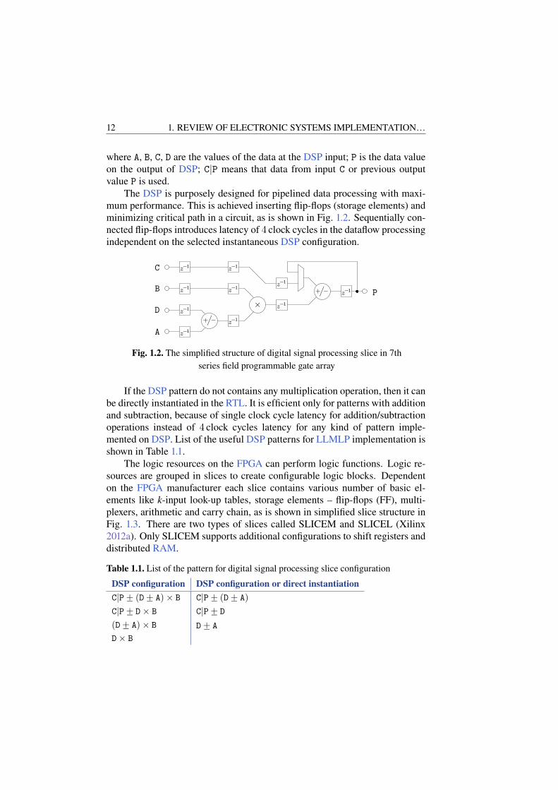
The DSP is purposely designed for pipelined data processing with maxi-mum performance. This is achieved inserting flip-flops (storage elements) andminimizing critical path in a circuit, as is shown in Fig. 1.2. Sequentially con-nected flip-flops introduces latency of 4 clock cycles in the dataflow processingindependent on the selected instantaneous DSP configuration.
A
B
C
D
P+/
−
+/
−
×
z−1z−1
z−1
z−1
z−1
z−1
z−1
z−1
z−1
z−1
Fig. 1.2. The simplified structure of digital signal processing slice in 7thseries field programmable gate array
If the DSP pattern do not contains any multiplication operation, then it canbe directly instantiated in the RTL. It is efficient only for patterns with additionand subtraction, because of single clock cycle latency for addition/subtractionoperations instead of 4 clock cycles latency for any kind of pattern imple-mented on DSP. List of the useful DSP patterns for LLMLP implementation isshown in Table 1.1.
The logic resources on the FPGA can perform logic functions. Logic re-sources are grouped in slices to create configurable logic blocks. Dependenton the FPGA manufacturer each slice contains various number of basic el-ements like k-input look-up tables, storage elements – flip-flops (FF), multi-plexers, arithmetic and carry chain, as is shown in simplified slice structure inFig. 1.3. There are two types of slices called SLICEM and SLICEL (Xilinx2012a). Only SLICEM supports additional configurations to shift registers anddistributed RAM.
Table 1.1. List of the pattern for digital signal processing slice configuration
DSP configuration DSP configuration or direct instantiation
C|P+− (D+− A)× B C|P+− (D+− A)
C|P+− D× B C|P+− D
(D+− A)× B D+− A
D× B

1. REVIEW OF ELECTRONIC SYSTEMS IMPLEMENTATION… 13
k-inputLUT Carry
chain
FF
FF
Rou
ting
wir
es
Rou
ting
wir
es
Slice
Fig. 1.3. The reconfigurable slice structure with look-up tables, carry chainand flip-flops in field programmable gate array
Due to the DSP sharing the intermediate calculation results must be storedin FPGA for fast access. To form small distributed memories in the latestFPGA each LUT in the SLICEM can be configured to the distributed 64 bRAM or ROM. All four LUT in a single SLICEM can form 256 b memoryformatted in various ways as single, dual or quad port RAM with asynchronousor registered output. To create a large buffers, the block RAM (BRAM) is used.BRAM can be configured as single or dual port RAM or ROM (Fig. 1.4).
BRAM1024×18
ADDRA[9:0]DINA[17:0]
WEACLKA
ADDRB[9:0]DINB[17:0]
WEBCLKB
DOUTA[17:0]
DOUTB[17:0]
Fig. 1.4. The interface of the configurable dual port block random accessmemory in field programmable gate array
The modern Xilinx FPGAs contains a hundreds of BRAM each 1024×18 bsize (Xilinx 2013d). Such blocks will be used to store synapse weights, for-ward/backward signals and trigonometric function values.
1.1.2. High Level Tools for Hardware Description LanguageGeneration
One of the main challenges in designs efficient implementation in FPGA isthe lack of the direct connection between algorithm design and hardware im-plementation. There can be hard to verify operation on chip against algorithm

14 1. REVIEW OF ELECTRONIC SYSTEMS IMPLEMENTATION…
specifications as hand coded HDL can bb error prone and hard to debug. Therecan also be differences between a fixed-point implementation and a floating-point specification of the algorithm. With different elements of the tool chainoften sourced from different vendors requiring multiple purchase request whichcan be difficult to budget. To address these challenges hardware designers of-ten looks at model-based design like Matlab and Simulink. HDL Coder allowsto convert the Simulink models and Matlab code (written in embedded Mat-lab form with restrictions) to HDL synthesizable code and testbenches (Math-Works 2013). Better performance is achieved using Xilinx System Generator(XSG) for DSP (Xilinx 2013b), because each block is a pre-optimized IP corefor Xilinx FPGAs. However, the cycle accurate scheduling nor resource shar-ing is hard to apply with XSG. Moreover, the XSG generated HDL code israther long and complex (Van Beeck et al. 2010).
The StateCAD allows to design of the state machines through graphicalinterface automatically generating synthesizable HDL code direct from the di-agram (Xilinx 2007). Despite that StateCAD reduces product developmentcost, this tool was removed since ISE Design Suite 11 version, because lack ofpopularity and support only on Windows platform.
The Matlab AccelDSP tool was used to map high-level described applica-tion to DSP slices for Xilinx FPGAs. It allows to generate synthesizable HDLsource with automated float to fixed-point conversion and testbench verifica-tion (Xilinx 2012b). Unfortunately, AccelDSP synthesis tool has been discon-tinued and is no longer available.
The commercial HLS tools C-to-Silicon, Catapult C, Synphony or VivadoHLS take a software description and turn it into effective hardware. Theirobjective is to generate hardware whose performance rivals with hand-writtendesigns. The advantage is that same design described in software can be reusedfor different FPGA (Cadence 2013). However, these tools have limitationswhen transforming sequential software to hardware. The high performance isachievable only for easy-to-pipeline algorithms with regular structure trivialfilters. As a proof, the favourite example is still the FIR filter (Xilinx 2015b).The performance of more irregular design with feedback loops and dynamicmemory allocations is rather poor.
First four HLS tools in Table 1.2 are model-based. It means, that designis assembled by hand from pre-compiled blocks and each of them has straightdefined reflection in the following RTL code. The required blocks must bemanually entered into the design. Therefore, designer must still worry aboutproper sequence of the block and compatibility of data type.
The HLS tools are very useful for quickly verification and validation ofthe algorithm in a hardware, when the design time is prior to the final designperformance. But till nowadays, for a greater design optimization we have to
1. REVIEW OF ELECTRONIC SYSTEMS IMPLEMENTATION… 15
Table 1.2. Comparison of high level synthesis tools
Tool Programming Generated
way/language code
HDL Coder Blocks RTL
XSG Blocks/Embedded-M RTL
LabView Blocks RTL
AccelDSP Blocks RTL
StateCAD State diagrams RTL/Abel
C-to-Silicon C/C++/SystemC RTLCatapult C C RTLSynphony C RTL
Vivado HLS C/C++ RTL/SystemC
hand code, despite the large choice of HLS tools, which significantly reducesFPGA design time at the cost of increasing latency or resource utilization. Themain advantages of the HLS design tools: fast implementation and verification,user friendly. Disadvantage: weak performance control, hard to meet of thetiming or resource constraints, complicated code readability.
Regarding the mentioned disadvantages the researchers are developing acustom HLS tool for a specific design implementation mainly based on dataand control flow graphs exploiting the design transformations (pipelining, re-timing, folding) for circuit performance optimization (Cong, Jiang 2008; Ka-zanavičius, Venteris 2000; Ronak, Fahmy 2012). The created tools are usedfor efficient mapping of mathematical expressions into DSP slices (Ronak,Fahmy 2014), mapping the Kahn processor network into DSP and FPGA ar-chitecture (Žvironas, Kazanavičius 2006) or targeting multiple application do-mains (Cong et al. 2011). Therefore, in the next section we will go through thespecifics of artificial neural network implementation on FPGA with the aim todistinguish suitable structures for further application in speech recognition.
1.2. Implementation of Artificial Neural Networksin Field Programmable Gate Array
Speech recognition systems work better if they are allowed to adapt to a newspeaker, the environment is quiet, and the user speaks relatively carefully. Anydeviation from these conditions will result in significantly increased errors.In most of the practical applications the speech is corrupted by a backgroundnoise (Chan et al. 2013; Yiu et al. 2014). This strongly degrades the accuracyof speech recognizers and makes it unpractical to use in applications that are

16 1. REVIEW OF ELECTRONIC SYSTEMS IMPLEMENTATION…
working in real conditions. Therefore, to make the FPGA-based recognizermore robust, many methods for noise cancellation are proposed, e.g., indepen-dent component analysis (Kim et al. 2003), spectral subtraction (Firdauzi et
al. 2013), adaptive filtering (Hadei, Lotfizad 2011; Thilagam, Karthigaikumar2015) or artificial neural networks (ANN) (Bosque et al. 2014; Er et al. 2005).
The adaptive filters in conjunction with multilayer perceptron (MLP) seemsto be attractive in speech enhancement application (Navakauskas 1999). SuchMLP can have finite impulse response (FIR), infinite impulse response (IIR)or lattice-ladder (LL) filters in a place of the neuron weights. These filterscan be employed for speech signal preprocessing and adaptive noise reduc-tion. The filter coefficients updating algorithm is well known and tested onPC applications. But since the IIR MLP (Back, Tsoi 1993) or lattice-laddermultilayer perceptron (LLMLP) (Navakauskas 2003) was firstly proposed, tillnowadays they are not implemented on FPGA. Therefore, our interest in thisthesis is the efficient LLMLP implementation on FPGA for the improvement ofspeech recognition. As LLMLP has same hardware implementation specificsas other ANN, thus the basic principles for mapping ANN algorithms to hard-ware structures are described below.
The FPGA has a suitable structure for pipelined and parallel ANN im-plementation. The main advantages of mapping ANN to FPGA are follow-ing (Misra, Saha 2010):
• The hardware offers very high computational speed at limited price.
• Provides reduced system cost by lowering the total component countand decreasing power requirements.
• The parallel and distributed architectures allow applications to con-tinue functioning with slightly reduced performance even in the pre-sence of faults in some components.
To obtain successful implementation of ANN, it is essential to have an un-derstanding of the properties of the ANN circuit to be implemented. For exam-ple, sensitivity to coefficient errors affects on signal quality, the final arithmeticbehavior affects the robustness of the algorithm and thereby its usefulness. Thecomputational properties of the ANN are also important, e.g., parallelism andmaximal sample rate affects the performance and implementation cost. Theseand other important specifics for efficient ANN implementation in FPGA areconsidered in following subsections.
1.2.1. Specifics of Artificial Neural Networks
Because of limited hardware resources the implementable ANN size and speedhighly depends on efficient implementation of the single neuron (Muthurama-

1. REVIEW OF ELECTRONIC SYSTEMS IMPLEMENTATION… 17
lingam et al. 2008). Therefore, the implementation of a large network on FPGAwith resource and speed trade-off is a challenging task. The main problem isin the replacing of floating-point numbers to the fixed-point. The input datamust be normalized in a range from 1 to −1 with restricted number of levels.Therefore, the limited accuracy plays significant role. The minimum 16 b forweights and 8 b for activation function inputs is good enough for applicationswith feed-forward ANN (Holt, Hwang 1993). The higher precision gives lowerquantization error. While higher speed, lower area and power consumption areavailable with lower bit precision. One of the disadvantage is a saturation, be-cause the range of weight×data product has fixed length (Moussa et al. 2006).Before implementation of any type of ANN in FPGA the issues presented inFig. 1.5 must be solved.
Precision. The recurrent part in the LLF alerts about growing error if thenumber of bits assigned to the signal is too low. Using the Xilinx IP coregenerator the maximum 64 b signal width is available. 16 b width connectionsin feed-forward pass of ANN are acceptable. The ANN with feed-back loopsrequires rather wide, i.e., 24–32 b, width signals and depends on accuracy de-mand for specific application.
Latency. The performance of whole ANN depends on the combinationaland sequential paths delay of the longest route in the synthesized circuit. Thebad HDL practice as asynchronous resets, adder threes instead of adder chains,incorrect synthesis tool settings, gated clocks, high number of nests within se-quential statements has become a bottleneck in aspiration of maximum fre-quency. The pipelined implementation gives the possibility to put a data to theinput of ANN synchronously at each clock. It is not always possible to imple-ment the ANN with feed-back wires in a pipelined way. Using of the variableshelps to merge a long arithmetic chain to easily be completed in a single clockcycle. But the longer the unregistered path in a chain, the lower the maximumfrequency in a final system. For the reasonable design at least 200–300MHzfrequency is expected and is possible with some serious scrutiny.
ANN FPGA implementation issues
Precision
Latency Resources
Test bench
Physical structureDescription level
Reconfigurability
Fig. 1.5. The hardware implementation issues of artificial neural network

18 1. REVIEW OF ELECTRONIC SYSTEMS IMPLEMENTATION…
Resources. The ANN requires a lot of arithmetic operations like summa-tion, multiplication and activation function stored in ROM. One DSP slice per-forms a multiplication of 18×25 b signals. The increase of precision requireshigher DSPs utilization rate, e.g., 32 b data multiplication utilizes 4DSP, 64 b –16DSPs. It is possible to use multipliers created from logic cells. In such case32×32 b multiplier uses 1088LUT6 and it is more than 2% of total numberof LUTs in e.g., ZynQ-7000 family xc7z020 FPGA. The limited number of re-sources makes it impossible to physically implement large ANN. In example,10-th order LLF utilizes all DSP slices in ZynQ-7000 Artix-7 FPGA. There-fore, physically implemented small part of ANN must share the resources tocreate larger network. Since the hardware complexity of a multiplier is pro-portional to the square of the word-length, a filter with more multipliers andsmaller word-length can sometimes be implemented with less hardware, thana filter with less multipliers and larger word-length. Therefore, the hardwarecomplexity of a digital filter should be determined carefully depending uponthe frequency specifications for LLF (Chung, Parhi 1996).
Test bench. To test the accuracy of the ANN various test bench files mustbe evaluated on the simulations first of all. It is important to check the networkprecision and weight dependence on different parameters as input signal, LLForder, number of layers, bit width of the data. All the results must be comparedwith the floating point precision ANN to get a relative error.
Physical structure. Limited resources do not allows physically implementwhole network. For example, the M -th order LLF with their learning algo-rithm utilizes at least 36×M + 4 DSP slices if 32 b signals are used. There-fore, it is more convenient to have few physical neurons and share them throughlarger virtual ANN (Misra, Saha 2010).
Description level. It is considered that VHDL and Verilog are the mainhardware description languages. They describe a circuit at low level, at thattime FPGA primitives are manually arranged in a design. The HDL givesus full performance and resource control. For inexperienced designers or forthose, who want to implement design quickly, there are a lot of high levelsynthesis tools, that will be described in next section. The HLS acceleratesFPGA design and verification time, but it hides the options to precisely managethe resource allocation and timing constraints.
Reconfigurability. The partial reconfiguration allows the modification ofan operating FPGA design by loading partial reconfiguration file, thus modi-fying ANN topology (Finker et al. 2013). The reconfiguration time is directlyrelated to the size of partial configuration file and usually takes less than asecond (Xilinx 2014b). We are interested not in the reconfigurability based onsupplementary file loading to FPGA, however on synchronous reconfigurationof DSP for new operation.

1. REVIEW OF ELECTRONIC SYSTEMS IMPLEMENTATION… 19
1.2.2. Artificial Neuron Structures
The artificial neuron is a mathematical model of biological neuron. The bodyof biological neuron is based on soma, which acts as the summation function.The input signals arrive in the soma from the dendrites (synapses). The outputof the artificial neuron is analogous to the axon of biological neuron. Eachtime when the soma reaches a certain potential threshold, the axon transmitsoutput signal to synapses of other neurons. Therefore, the axon is analogous tothe activation function in artificial neuron.
There are two different neuron configuration in a hardware (Omondi et al.
2006): tree (Fig. 1.6a) and chain (Fig. 1.6b). The trade-off is between process-ing latency and efficient use of logic resources. With a tree configuration theuse of slice logic is quite uneven and less efficient than with a chain. If numberof inputs is large, then a combination of these two approaches is used. Such areservation of a single DSP for one synapse allows to implement parallel ANNstructures, which size is highly limited by FPGA internal interconnection re-sources. The number of available synapses is also restricted by the number ofDSP. In Fig. 1.6 presented neuron is suitable for small and fast ANN structureswith a pipelined input. The activation functions can be implemented as polyno-mial approximations, CORDIC algorithm, table-driven method. For hardwareimplementation the trade-off between accuracy, performance and cost are allimportant.
It is often unnecessary to have such ANN, that captures data at each risingedge of clock. Therefore, it is possible to use one multiplication (DSP slice)to compute the product and summation of each weight×data operation in a se-quential manner (Fig. 1.7). In this case, the latency is proportional to the num-ber of synapses in each neuron. Such a model of neuron is popular in a hard-ware implementation of the feed-forward neural network, i.e., MLP (Ferreiraet al. 2007; Muthuramalingam et al. 2008). The structure of MLP with parallelneural unit that calculates 32 products at each clock cycle is proposed (Lotrič,Bulić 2011).
The precision of the activation functions plays a significant role especiallyif the number of hidden layer in the MLP is high. It is possible to implementthe sigmoid function in a simplified manner replacing e−x with 1.4426×2−x
and splitting the x into whole number and fractional part (Muthuramalingamet al. 2008). Such approach needs a 100 cycles to implement an activationfunction. Therefore, the look-up tables are proposed to use as a faster way fornonlinearity estimation.
An important problem for designers of FPGA-based ANN is a proper se-lection of the ANN model suitable for limited hardware resources. A compar-ative analysis of hardware requirement for implementing MLP in Simulink and

20 1. REVIEW OF ELECTRONIC SYSTEMS IMPLEMENTATION…
data 3weight 3
data 2weight 2
data 1weight 1
data 0weight 0
Mul
Mul
Mul
Mul
Sum
Sum
Sum
Sum Activationfunction result
a) The tree configuration
data 3weight 3
data 2weight 2
data 1weight 1
data 0weight 0
Mul
Mul
Mul
Mul
Sum
Sum
Sum
Sum Activationfunction result
b) The chain configuration
Fig. 1.6. Two distinct implementation of the neuron: the tree a) and chain b)configurations
dataweight
MAC
Mul Sum result
Fig. 1.7. Digital neuron model based on multiply-accumulate (MAC) unit
translating to hardware indicates that the not complex spiking neural network(SNN) is a most appropriate model for non-linear task solving in a FPGA (John-ston et al. 2005). The reason is a type of neuron. The spiking neuron do notuses multipiers in a synapses, however only addition and threshold operationsare required. Any FPGA always has more configurable logic blocks with sum-mation and comparison operators than DSPs. Therefore, SNN is more areaefficient and relatively easier to construct than any other ANN. However, it ismuch harder to develop a model of SNN with stable behavior that computes aspecific function (Carrillo et al. 2012). Moreover, current FPGA routing struc-tures cannot accommodate the high levels of interneuron connectivity inherentin complex SNNs (Harkin et al. 2009).

1. REVIEW OF ELECTRONIC SYSTEMS IMPLEMENTATION… 21
1.2.3. Dynamic Neuron
Regardless of the type of ANN, the synapse of a neuron always plays a mean-ing role, since its ability to adapt. For the processing of a time-varying signalsusually it is useful to replace a single weight synapse with a band-pass filterof the desired order. Therefore, associated dynamic neuron training algorithmbecomes more sophisticated especially if infinite impulse response filters areused. When the direct structure of such filter is selected the number of param-eters to be adapted becomes proportional to 2M + 1, where M is the filterorder (usually M is set the same for the synapses of particular layer). Howeverthe main disadvantage of such dynamic neuron training implementation liesin the elaborated control of filter stability during the learning process. Thusthe rearrangement of the filter to the lattice-ladder structure with the simpleststability check (Regalia 1995) is appealing for the implementation.
The presented neurons (Fig. 1.6 and 1.7) will be dynamic if the synapsesare replaced by filters. One of the possible filter is the LLF presented inFig. 1.9. Each section of the LLF consists of a normalized lattice autoregressive-moving average filter. The local flow of information in the lattice part of filterfor j section is defined by:
[fj−1(n)bj(n)
]=
[cosΘj − sinΘj
sinΘj cosΘj
] [fj(n)
z−1bj−1(n)
]; (1.2)
sout(n) = Φ
(M∑
j=0
bj(n)vj
), (1.3)
with initial and boundary conditions b0(n) = f0(n) and fM (n) = sin(n),where sin(n) – input signal; vj(n) – weights of the ladder; Θj – rotation anglesof the lattice; fj(n) and bj(n) – forward and backward signals of the lattice,correspondingly; s(n) – the output of the LLN with N inputs and M th orderLLF as its synapses; Φ{�} – neuron activation function.
fj(n)
bj(n)
fj−1(n)
bj−1(n)cosΘj
cosΘj
sinΘj sinΘj
Θj
z−1
Fig. 1.8. The structure of normalized lattice section used in Fig. 1.9presented lattice-ladder filter

22 1. REVIEW OF ELECTRONIC SYSTEMS IMPLEMENTATION…
In a time-varying environment the normalized lattice filter is superior overother lattice forms with one, two or three multipliers (Gray, Markel 1975).Contrary each normalized lattice section requires four times more multiplica-tion operations when compared to a single multiplier lattice for the cost ofstability. It could be shown that equality:
∣∣fj−1(n) + ibj(n)∣∣ =
∣∣fj(n) + ibj−1(n− 1)∣∣, (1.4)
holds for all j sections (Gray, Markel 1975). Therefore, the normalized latticefilter requires only the starting point to be stable and any truncation of the filtercoefficient don’t moves poles outside the unit circle. Thus there is no need tocheck lattice stability for normalized lattice filter.
cosΘM
cosΘM
cosΘM−1
cosΘM−1
cosΘ1
cosΘ1
sinΘMsinΘM−1 sinΘ1
vM vM−1 vM−2 v0
sin(n)
sout(n)
sinΘM sinΘM−1 sinΘ1
z−1z−1z−1
Fig. 1.9. The critical path in the M -th order lattice-ladder filter
The unregistered critical path in the LLF is marked by a gray color inFig. 1.9. In the LLF the computation time delay in critical path is proportionalto the filter order M and equal to (M + 1)×2. The longer the critical path,the higher delay is between the synapse input sin(n) and the synapse outputsout(n). If this filter will be implemented as is, its maximal clock frequencydegrades drastically, because of the growing filter order M . In order to achievehigher performance the LLF can be pipelined through retiming and interleav-ing procedures (Chung, Parhi 2012; Parhi 2013). Such a circuit manipulationprocedures are indeed helpful for pipelining a design without feedbacks, ifthere is no input sin(n) = f
(sout(n)
)dependence on the output sout(n). The
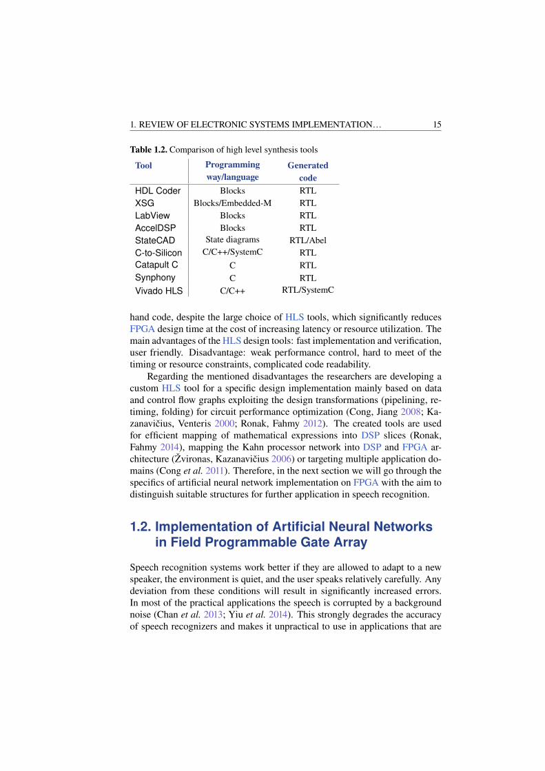
M th order LLFs (Fig. 1.9) are used as synapses in artificial neurons. Theneurons distributed in parallel construct a single layer of MLP presented inFig. 1.10. The MLP consists of multiple layers, with each layer fully connectedto the next one. A lattice-ladder multilayer perceptron (LLMLP) is defined bynumber of layers L, number of neurons in each layer {N (0), N (1), . . . , N (L)}and filter orders {M (0),M (1), . . . ,M (L)}. The input layer denotes the numberof features/dimensions in the input signals. The number of outputs in LLMLP
1. REVIEW OF ELECTRONIC SYSTEMS IMPLEMENTATION… 23
s(1)1 (n)
s(1)2 (n)
s(1)3 (n)
s(1)
N(1)(n)
s(L)1 (n)
s(L)2 (n)
s(L)3 (n)
s(L)
N(L)(n)
Input layer Second layer Hidden layer L-th layer
Fig. 1.10. Representation of multilayer perceptron
is directly related with number of neurons in the last Lth output layer. All thelayers arranged between input and output layers are hidden.
1.2.4. Training of Dynamic Neuron
Development of the lattice version of the gradient descent algorithm followsthe same methodology as for the direct form. The output error δ is differenti-ated with respect to the filter parameters sinΘM , cosΘM , to obtain negativegradient signals ∇ΘM
. The main advantage of the lattice form over the di-rect form is related with LLF stability. The LLF is inherently stable for time-varying signals (due to the fact that sinΘM ≤ 1, cosΘM ≤ 1), while thedirect form is not (Regalia 1995). Synapse presented in Fig. 1.9 has to learn Θj
and vj parameters using simplified gradient descent training algorithm, whenweight updates are expressed:
Θj(n+ 1) = Θj(n) + µδ∇Θj(n); (1.5)
vj(n+ 1) = vj(n) + µδbj(n); (1.6)
δ =(1− sout(n)
2)e(n), (1.7)
here µ – a training step; δ – an instantaneous output error; e(n) = s⋆out(n) −sout(n) – error between desired s⋆out(n) and output signal sout(n); ∇Θi,j
– gra-dients of lattice weights; bj(n) – backward signal inside of lattice.
There are in total 14 possible ways how to exactly implement order recur-sion required for gradient training algorithm (Navakauskas 2003). And onlyfour of them (t3, t4, t11, t12) have a straightforward implementation, as isshown in Fig. 1.11 and Fig. 1.12. That is justified by the fact that the otherten remaining cases have one or several un-implementable advanced opera-tors. The dashed boxes separates the “main order” calculations from the cal-culations involved with the delays and additional signals going from latticepart of the LLF. The gradients ∇Θj
of lattice weights are estimated by cir-
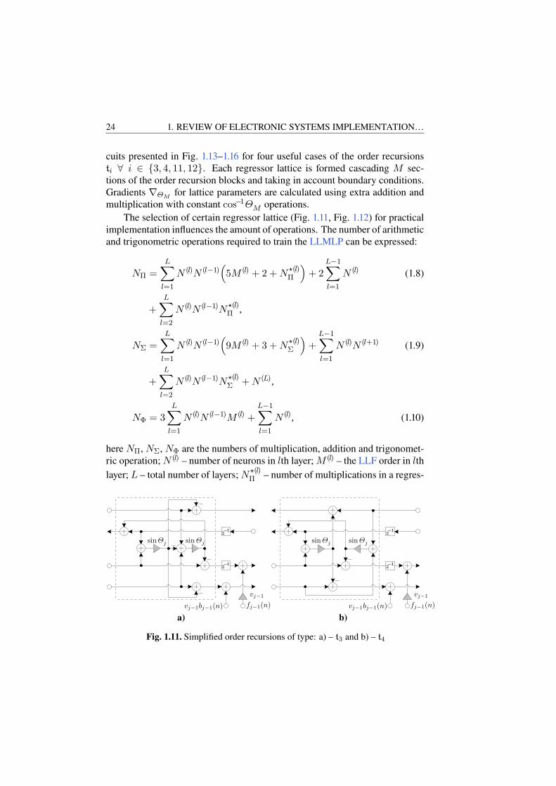
24 1. REVIEW OF ELECTRONIC SYSTEMS IMPLEMENTATION…
cuits presented in Fig. 1.13–1.16 for four useful cases of the order recursionsti ∀ i ∈ {3, 4, 11, 12}. Each regressor lattice is formed cascading M sec-tions of the order recursion blocks and taking in account boundary conditions.Gradients ∇ΘM
for lattice parameters are calculated using extra addition andmultiplication with constant cos−1ΘM operations.
The selection of certain regressor lattice (Fig. 1.11, Fig. 1.12) for practicalimplementation influences the amount of operations. The number of arithmeticand trigonometric operations required to train the LLMLP can be expressed:
NΠ =L∑
l=1
N (l)N (l−1)(5M (l) + 2 +N
⋆(l)Π
)+ 2
L−1∑
l=1
N (l) (1.8)
+L∑
l=2
N (l)N (l−1)N⋆(l)Π ,
NΣ =L∑
l=1
N (l)N (l−1)(9M (l) + 3 +N
⋆(l)Σ
)+
L−1∑
l=1
N (l)N (l+1) (1.9)
+L∑
l=2
N (l)N (l−1)N⋆(l)Σ +N (L),
NΦ = 3L∑
l=1
N (l)N (l−1)M (l) +L−1∑
l=1
N (l), (1.10)
here NΠ, NΣ, NΦ are the numbers of multiplication, addition and trigonomet-ric operation; N (l) – number of neurons in lth layer; M (l) – the LLF order in lth
layer; L – total number of layers; N⋆(l)Π – number of multiplications in a regres-
a
b
c
d
sinΘjsinΘj
vj−1
vj−1bj−1(n) fj−1(n)
z−1
z−1
a)
a
b
c
d
sinΘjsinΘj
vj−1
vj−1bj−1(n) fj−1(n)
z−1
z−1
b)
Fig. 1.11. Simplified order recursions of type: a) – t3 and b) – t4

1. REVIEW OF ELECTRONIC SYSTEMS IMPLEMENTATION… 25
sinΘjsinΘj
sinΘj cosΘj
fj(n)
vj−1
vj−1bj−1(n)
z−1
z−1
a)
sinΘjsinΘj
sinΘj cosΘj
fj(n)
vj−1
vj−1bj−1(n)
z−1
z−1
b)
Fig. 1.12. Simplified order recursions of type: a) – t11 and b) – t12
Θ1Θ2ΘM
Θ⋆1Θ⋆
2Θ⋆
M
vM v1 v0
vM v1
cos−1ΘM cos−1Θ1
∇ΘM(n) ∇Θ1
(n)
sin(n)
sout(n)
z−1
z−1
z−1
z−1 z−1
Fig. 1.13. The connected circuit of lattice-ladder filter and t3 type regressorlattice for ∇Θj
(n) gradients estimation
sor in the lth layer; N⋆(l)Σ – number of additions in a regressor in the lth layer.
Both parameters N⋆(l)Π and N
⋆(l)Σ depend on the regressor type as summarized
in Table 1.3. Despite that regressor lattices t3 and t4 need sinΘj , cos−1Θj and
alike t11 and t12 need sinΘj , cosΘj , cos−1Θj trigonometric functions to be
calculated for each order recursion, the total number of trigonometric opera-tions OΦ is same for all regressor lattice types ti (last row in Table 1.3). Eachadditional order recursion in ti requires only cos−1Θj calculation, since sinΘj ,cosΘj are computed in primary lattice and results are shared with regressorlattice. The total number of operation necessary for LLMLP implementationin conjunction with weight adaptation is summarized in Table 1.4.

26 1. REVIEW OF ELECTRONIC SYSTEMS IMPLEMENTATION…
Θ1Θ2ΘM
Θ⋆1Θ⋆
2Θ⋆
M
vM v1 v0
vM v1
cos−1ΘM cos−1Θ1
∇ΘM(n) ∇Θ1
(n)
sin(n)
sout(n)
z−1
z−1
z−1
z−1
z−1 z−1
Fig. 1.14. The connected circuit of lattice-ladder filter and type t4 regressorlattice for ∇Θj
(n) gradients estimation
Θ1Θ2ΘM
Θ⋆1Θ⋆
2Θ⋆M
vM v1
v0
v0
vM v1
cos−1ΘM cos−1Θ1
∇ΘM(n) ∇Θ1
(n)
sinΘ1sinΘM
cosΘ1cosΘ2
sin(n)
sout(n)
z−1
z−1
z−1
z−1
z−1 z−1
Fig. 1.15. The connected circuit of lattice-ladder filter and type t11 regressorlattice for ∇Θj
(n) gradients estimation
The newest FPGA contains up to 3600DSP blocks dedicated for multi-plication and addition (Xilinx 2014a). The parallel implementation of largeLLMLP is restricted by limited arithmetic resources. Therefore, the LLMLPwith only few neurons and low order LLF can be implemented in single FPGA

1. REVIEW OF ELECTRONIC SYSTEMS IMPLEMENTATION… 27
Θ1Θ2ΘM
Θ⋆1Θ⋆
2Θ⋆M
vM v1
v0
v0
vM v1
cos−1ΘM cos−1Θ1
∇ΘM(n) ∇Θ1
(n)
sinΘ1sinΘM
cosΘ1cosΘ2
sin(n)
sout(n)
z−1
z−1
z−1
z−1
z−1 z−1
Fig. 1.16. The connected circuit of lattice-ladder filter and type t12 regressorlattice for ∇Θj
(n) gradients estimation
Table 1.3. The total number of operations for lattice-ladder filter and regres-sor
Mathematical Single Single regressor of type
calculations LLF t3 t4 t11 t12
Multiplications, N⋆Π 5M + 1 4M 4M 6M + 1 6M
Additions, N⋆Σ 3M 10M − 1 9M − 1 10M − 2 11M − 3
Trig. functions, N⋆Φ 2M 1M 1M 1M 1M
Table 1.4. The total number of operations for different lattice-ladder multi-layer perceptron sizes
N (l) M (l) NΠ NΣ NΦ
2-2 2 220 230 481-10-1 4-6 1620 1961 3102-10-1 4-6 2170 2531 430
1-10-10-1 2-4-6 8480 10981 14605-10-10-1 2-4-6 9640 12141 1700
without resource sharing. Obviously the DSP slice sharing through time isnecessary for large LLMLP implementation. To solve the issues of large ANNimplementation on restricted FPGA, the researchers invoke the high or lowlevel approaches.

28 1. REVIEW OF ELECTRONIC SYSTEMS IMPLEMENTATION…
1.2.5. Indirect (High Level) Approach
The implementation of desired ANN in a high level is a fastest way from theprogrammer point of view to code the ANN equations and take less care aboutphysical ANN structure. Many researchers applied their own written toolsin C, Matlab or others high-level languages to implement desired ANN onFPGA in a convenient way. In most cases the tools generate VHDL or RTLoutput files, that exactly describe the ANN in a lower level. Afterwards theFPGA vendors synthesis, mapping and PAR tools are used. It is popular touse Simulink tool in combination with Xilinx system generator as a high leveldescription of ANN (Oniga et al. 2008). The advantage of Simulink applicationis a fast description time of ANN at the expense of final circuit performance.
A special program is developed in C++ to automatic generation of VHDLcode of the ANN (Dinu et al. 2010), while each neuron is represented as specialcase of Boolean function. The parameters of ANN are feed to the C++ programas a matrices in text file. The Matlab is used to develop MLP VHDL IP corewhich can run a network with 2 hidden layers, 128 neurons and 31 inputs foreach neuron (Rosado-Munoz et al. 2008). The generated VHDL files containsthe generate instruction and generic parameters, which are customizable aftergeneration of IP core. Every single neuron have a multiply-accumulate (MAC)structure (Fig. 1.7) and makes calculation in pipeline.
The support vector machine (SVM) IP core compiler was developed in aC# language to generate the VHDL files (Anguita et al. 2011). In a created GUIit is able to configure the SVM to desired precision, choose a number of sup-port vectors and many others parameters. To solve the quadratic programmingproblem the sequential minimal optimization was used. The SVM uses fixed-point arithmetic, therefore can be implemented on resource-constrained hard-ware (Anguita et al. 2008). The SVM achieves 6 % classification rate whileusing 12 b for coefficient and kernel precision. The lowest 6 cycles latencyis achieved using linear piecewise kernel architecture. The highest 15 cycleslatency gives a CORDIC-like kernel.
The automatic VHDL files generator for self-organizing features map wasdeveloped in (Onoo et al. 2009). The network size problem is solved intro-ducing physical and logical neuron concept when the size of desired neuralnetwork is larger than available FPGA resources (Yamamoto et al. 2011). Thephysical neurons sequentially executes the logical neurons. The advantage isin smaller circuit size, but the execution time is longer. The Simulink basedapproach for self-organizing features map with on-chip learning implementa-tion was developed (Tisan, Cirstea 2012). Two DSP slices are hardwired tounique neuron, so the maximal network size is determined by available FPGAresources.

1. REVIEW OF ELECTRONIC SYSTEMS IMPLEMENTATION… 29
All the mentioned ANN implementation approaches reduce the designtime, because network structure is described in a high-level language. But it isstill unknown, whether the network has an optimal composition in the physicalcircuit. This issue is considered in next subsection.
1.2.6. Direct (Low Level) Approach
Towards the direct ANN implementation in FPGA at the RTL level the caremust be taken firstly about limited arithmetic resources. Therefore, instead ofimplementing a complete network it is advisable to implement only the singlelargest layer. Afterwards, combine the entire ANN using the layer multiplex-ing and some control logic (Himavathi et al. 2007). Instead of dedicating amultiplication operator for each synapse, a DSP slice configured to MAC canprocess all the inputs of neuron in serial (Savich et al. 2007). The use of FPGApartial reconfigurable areas reduce resource usage by dynamically insertingand removing neuron blocks on the network and this way configure MLP withdifferent topologies (Alberto de Albuquerque Silva et al. 2015).
If multiplication operation has to be implemented in DSP48E1 slices onXilinx FPGA, then the maximum 25×18 b width input product can be achievedutilising single DSP slice Xilinx (2014a). The higher precision requirementscan be satisfied in two ways: by time-multiplexing of a single DSP slice (how-ever that will increase a total latency of the system) or by the use of two DSPslices (however that will consume DSP slices very fast).
One of the most important issue in the hardware-based ANN is the im-plementation of nonlinear activation functions such as sigmoid (Nambiar et
al. 2014), logarithmic sigmoid (Vaitkus et al. 2014) or hyperbolic tangent (Ba-houra 2014). Such functions have easily computed derivative, which is im-portant for training process, because that decreases the computational load.However, the precise implementation of the nonlinearity in FPGA gives causefor concern. The reasonable solutions while solving this issue can be: com-binational (Tommiska 2003; Zamanlooy, Mirhassani 2014), piecewise linear(PWL) (Armato et al. 2011; Ferreira et al. 2007) or quadratic (PWQ) approx-imations (del Campo et al. 2013; Nambiar et al. 2014), look-up tables (LUT)synthesized in a logic (Gomperts et al. 2011; Lotrič, Bulić 2012) or storedin on-chip memory (Bahoura 2014). The straightforward implementation ofnonlinear function in hardware is not a correct approach, because both expo-nentiation and division are logic and arithmetic resource hungry operations(Gomperts et al. 2011; Tommiska 2003). The CORDIC algorithm introduceslatency and has limited input domain (Armato et al. 2011).
Efficient FPGA implementation of activation function is a multi-criteriatask. The balancing of the accuracy, resources and processing speed must be

30 1. REVIEW OF ELECTRONIC SYSTEMS IMPLEMENTATION…
considered (Armato et al. 2011). High precision requires more resource. Signalrouting through high amount of logic is a bottleneck to achieve higher clockfrequency for the synthesized design, due to the growing delay in a critical pathof not compact hardware. Moreover, resource reduction makes circuit faster,but also influences inaccuracy in approximated activation function.
When only few bits are used as the input of activation function, then itmakes sense to use combinational approximation based on direct bit level map-ping, that doesn’t requires any arithmetic operators. The bit level mappingmethod was proposed in (Tommiska 2003). It is shown that with 6 b precisionthe maximal absolute error of the activation function is less than 1%.
The polynomial approximation methods are based on the function inputrange division into equal parts, where each function subinterval is approxi-mated by line or curve (Armato et al. 2011). The PWL approximation of hy-perbolic tangent with 256 linear sections provides a maximum error of 0.002%using 32 b arithmetic (Ferreira et al. 2007). The controlled accuracy second or-der approximation of sigmoid function was implemented on single DSP slicewith maximum allowable 1% error (del Campo et al. 2013). The amount ofadditional logic resources changes depending on the required word-length anderror. The PWQ approximation can be implemented by reusing already uti-lized multiplier and adder units in neuron block proposed in (Nambiar et al.
2014). The main disadvantage of polynomial approximation technique is theincreased latency due to the growing number of multiplication operations forthe higher-order polynomial. The maximum allowable 2% error with 9 b inputis achieved using hybrid PWL and LUT methods in (Meher 2010) implement-ing hyperbolic tangent function in hardware.
The LUT-based approach works much faster than polynomial approxima-tion, since LUT consumes memory. Small LUT is usually implemented indistributed memory, which does not require delay units, but has a limited size(Bahoura 2014). Newest FPGA chips have at least 0.5MB of on-chip blockRAM (BRAM) with one clock cycle latency to access stored data (Xilinx2013c). Therefore, large LUT is generally stored in BRAM. The accuracy ofapproximated hyperbolic tangent under various precision input signal and LUTsize was investigated in (Gomperts et al. 2011). Depending on the applicationand required accuracy for the activation function, different sizes LUTs from28 samples (Lotrič, Bulić 2012) to 215 samples (Bahoura 2014) are used.
The description in the literature of limits for accuracy of activation func-tion is fragmented and it lacks commonly acceptable values. The average ǫavg
and maximum ǫmax error values usually depend on the precision requirementsfor the application and in many cases maximum error 0.4% (Sledevič, Nava-kauskas 2016), 1.5% (Armato et al. 2011) or even 2% (Meher 2010; Zaman-looy, Mirhassani 2014) is tolerable.

1. REVIEW OF ELECTRONIC SYSTEMS IMPLEMENTATION… 31
The more common way to implementing the nonlinear function in currentFPGA-based neural network is to have a LUT. Using nowadays FPGA thereis not much concern about random access memory, therefore LUT stored inBRAM is advantageous and will be used in our implementation.
1.2.7. Artificial Neural Network Chips
The neurochip always contains a weight×input multiplication and their sum-mation blocks. The other blocks for neuron state, activation function, weighsloading controllers can be on or off chip. There are several categories of dedi-cated chip:
• Bit-like – first neurochips constructed from cheap building blocks (sin-gle neurons) with off-chip learning possibility and from few to dozensof neurons and synapses on single chip (Mauduit et al. 1992; MD1220Neuro Bit Slice; NLX-420 Datasheet).
• Single instruction multiple data (SIMD) neurochip run the same in-struction simultaneously on multiple processing elements (PE) withdifferent data for each PE. The number of PEs in single chip variesfrom 16 to 64 (Hammerstrom 1990; Kim et al. 2005; Means, Lisenbee1991).
• In the systolic array each PE process instructions synchronously withother PEs and the result from first layer is passed to each next layerin the pipelined manner. The array structure is well matched to ANNhaving potentially high utilization ratio of the processing unit becausethe multiplier in each synapse has maximal load (Amin et al. 1999;Chung et al. 1992; MA16 Technical Report). The main disadvantagesof the systolic PE stucture are: the complex array interfacing and syn-chronous weight update control.
Different ANN design evaluation in a short time, reasonable cost and re-duced hardware development cycle bring FPGA to effective programmable re-sources for ANN implementation. Partial and online reconfiguration providesoftware like flexibility and additional advantages. In contrast to VLSI the cir-cuit density is still lower in the FPGA and it restricts the implementation oflarge scale ANN with thousands of neurons.
A potential issue with implementing a ANN in FPGA is the limited amo-unt of routing resources (Misra, Saha 2010). Unlike the logic resources (flip-flops, look-up tables or memory blocks), routing resources are difficult to quan-tify. The growing ANN hits the routing limits very quickly. Place and routeprocess takes longer to fit the ANN into FPGA and it creates a connectionsthrough logic cells if available routing resources are insufficient. Therefore,

32 1. REVIEW OF ELECTRONIC SYSTEMS IMPLEMENTATION…
most of the researchers takes this approach and choose on hardware implemen-tation of several neurons only for bigger virtual ANN creation using schedul-ing and multiplexing in time. Having just one physical layer of neurons re-duces hardware requirements (Nedjah et al. 2009). Such a technique requiresadditional amount of memory to store connectivity weights and intermediateresults. The big issue is to write a scheduler, which keeps memory buses satu-rated in order to achieve maximal throughput.
The direct register transfer level approach is more advantageous againstANN implementation in high-level of abstraction. From programmers point ofview, one of the fastest and easiest way for efficient implementation of ANNin FPGA is to use well known HDL and describe the net as a set of equa-tions. Then put this set to the circuit design chain and finally only remainsto hope that synthesizer, mapper, placer-and-router will give optimal circuit.The vendor standard FPGA design tools are general purpose, therefore havea global resource, power or latency optimization goals. Consequently, we arenot guaranteed, that ANN optimally fits constrained hardware after the finalPAR stage. The direct low-level ANN implementation gives full control ofprimitives and their routing, but requires additional knowledge about internalstructure of slices and routing resources. In the design chain each additionalcircuit conversion step brings uncertainty to final structure. The closer theANN description is to FPGA primitive building block, the more efficient net-work deploying can be achieved.
The main FPGA vendors provide design software suite with special tools –editors for already placed and routed designs (Altera 2013; Xilinx 2013a).These tools as a rule are dedicated for timing and routing analysis. The man-ual optimization of already routed circuit is a bad practice, since the timingrequirement is still not guaranteed and rather become worse (Clayton 2008).
1.2.8. Efficiency Criteria of Neural Network Hardware
The ANN are generally described in terms of topology, learning algorithm, ac-tivation function, number of processing elements, layers, the type and numberof inputs/outputs. The ANN implemented in FPGA are additionally specifiedby data representation, precision, weight storage, synaptic connection (hard-wired or programmable), and on-chip learning possibility. Considering thementioned parameters many ANN performance ratings are proposed and threeof them are commonly used (Misra, Saha 2010):
• The processing speed measured in connections per second. It is a rateof multiplication, addition and activation function computation andshows how well the chosen network fits the hardware architecture.

1. REVIEW OF ELECTRONIC SYSTEMS IMPLEMENTATION… 33
• The learning speed measured in connection updates per second. It in-dicates the weights updating rate and measures the amount of samplesto learn.
• The average energy in watt per synapse needed to compute and updatethe synapse.
Despite above mentioned main performance measurement rates, more hard-ware specific criteria exist:
• Reconfigurability number defined as the size of the set of all imple-mentable but different net topologies.
• Effective connection primitives per second provides improved measureof processing speed, which takes into account input and weight accu-racy in bits (van Keulen et al. 1994).
• The algorithmic efficiency is measured as an impact of the hardwareconstraints on the convergence of learning error in various ANN struc-tures implemented in neurochip (Cornu, Ienne 1994).
• Nonlinear functions implemented in a hardware consumes time andarea resources. The overhead of the activation function (AF) suggeststo use LUTs (Hammerstrom 1990; Noory, Groza 2003) or piecewiselinear functions for the approximation (Amin et al. 1997). An exper-imental study on the precision requirements denotes that 16 b is suf-ficient for the encoding of AF (Holt, Hwang 1993). The AF interpo-lation by Taylor series allows to decrease the number of LUT savingrelatively high accuracy (Beiu 1998).
• The synaptic storage density plays significant role especially in largescale ANN, when trade-off must be achieved between memory sizeand power consumption. The type of memory. The distributed RAMprovides high density, but consumes more power. On the other handstatic RAM consumes less power with 4 times worse memory den-sity (Misra, Saha 2010).
• The Quality of Results (QoR) is the most often meaning of the maxi-mum clock frequency, at which a given design must operate in a spe-cific FPGA. QoR is an indicator of critical path performance, which ishighly related with the timing constraints, coding style and PAR tool.
The mentioned criteria are usually valuated independently on one another.However, e.g., the acceleration of synaptic processing or learning speed throughparallelization of ANN structure yields the growth of FPGA resource utiliza-tion. Therefore, optimization by one individual objective makes any other indi-vidual worse. The lack of multi-objective analysis of ANN implementation inFPGA allows to lead out new criteria taking into account conflicting require-ments.

34 1. REVIEW OF ELECTRONIC SYSTEMS IMPLEMENTATION…
1.3. Implementation of Speech Recognition inField Programmable Gate Array
Nowadays people spend more and more time interacting with many electronicdevices installed at their homes, working places, transportation vehicles, otherpublic places. Therefore, human machine communication is a hot researchtopic. Speech is a natural and one of the easiest means for humans to use forcommunication and information exchange. Reliable and fast device controlby speech can strongly facilitate everyday life of people. Therefore, a lot ofresearch efforts are directed towards improvement of the speech recognitionaccuracy and the recognition speed.
Despite of recent software-based Lithuanian speech recognition (Lileikytė,Telksnys 2011) and synthesis (Pyz et al. 2012) implementations on personalcomputers and servers there is an unaddressed need of embedded systems formobile and stand-alone devices, interactive voice controlled systems, disabledperson equipment, etc. Embedded systems bring in their specific requirementsfor speech recognizers: the limited speed of processing, the limited size of me-mory, the low power consumption. The recognition of large vocabulary andcontinuous speech requires complicated algorithms with huge amounts of cal-culations, large quantities of memory (Choi et al. 2010; Veitch et al. 2010).This can result in enlarged power consumption, longer recognition time andhigher recognition error rate.
Many automatic speech recognition systems for the languages of minoruse are now developed. Presented in (Martinčić-Ipšić et al. 2011) Croatianspeech recognizer uses acoustic models based on context-dependent triphonehidden Markov models (HMM) and phonetic rules. Experimentally it is shownthat the system can be used for speech recognition with word error rate below5%. In (Sojka et al. 2004) a speaker independent speech recognition systemfor Estonian language is described. Clustered triphones with Gaussian mix-ture components are used there for acoustic modelling. The error rate of thesystem is improved to 27.3%. In (Hirsimaki, Kurimo 2004) Finnish speechrecognition based on sub-word decoders is presented. The pursued task was tofind the most probable HMM state sequence. The word error rate there is de-creased up to 32% for very large vocabulary. For Czech speech recognition in(Prochazka et al. 2011) investigation on usability of publicly available n-gramcorpora to create Czech language models is carried out. The experiments onlarge test data illustrate the impact of Czech as highly inflective language onthe perplexity. The best achieved average error rate is 20%. The multi-lingualItalian – Lithuanian small vocabulary speech recognition is implemented usingmultilingual transcription in (Maskeliūnas, Esposito 2012). The average recog-

1. REVIEW OF ELECTRONIC SYSTEMS IMPLEMENTATION… 35
nition accuracy of ten spoken numbers for the Lithuanian language is 93% andfor the Italian – 98%. It is important to acknowledge that all above analysedspeech recognizers are implemented in software.
In some cases the robustness and correctness of recognition, together withthe low power consumption are preferred against the size of the vocabulary(Zhang et al. 2011). Then the natural choice is an isolated word recognitionapproach leading to lower hardware requirements: much smaller vocabulary(less memory), simpler classification (lower speed and power consumption),potentially higher recognition rate (correctness), and at the same time an abilityto use advanced noise cancellation (robustness) (Stašionis, Serackis 2011).
The FPGA platform lets to employ the parallelization and pipelining tech-nique in speech recognition. It is a flexible architecture to develop systems incomparison to implementations on the ASIC devices. The embedded processor-based solutions on the market have an average 80% recognition rate and lim-ited size of the dictionary: 32 (EasyVR (Chakravarty 2014)) or 75 (NLP (Sen-sory 2012)) commands. The main issue in such recognizer is to ensure real-time requirements for the speech recognition (especially at the features com-parison stage). Contrary for this approach the implemented features extractionand matching processes can run independently in FPGA (Choi et al. 2010),(Veitch et al. 2010), (Zhang et al. 2011), (Pan et al. 2011) or GPU (Sart et al.
2010), (Zhang et al. 2012).First soft-core implementations on Virtex-4 family FPGA of Lithuanian
isolated word recognizer were done by Electronic Intelligent System group inVGTU Electronic Faculty (Arminas et al. 2010). The use of soft-core proces-sor MicroBlaze together with intellectual property cores for signal processingenables to accelerate word recognition process by 1.55 times (Ivanovas 2012;Tamulevičius et al. 2010), however it was still not enough for a real-time oper-ation.
The common speech recognition algorithm consists of several steps, asshown in Fig. 1.17. The speech signal can be loaded from memory or capturedfrom microphone in a real-time. The preprocessing step involves the noise re-duction and signal partitioning into equal overlapped 10–30ms frames. Foreach frame the features vector is formed employing predictive or cepstral anal-ysis. The extracted features are compared with the features stored in dictionary.If both vectors of features match each other a concrete command related withrecognized word is executed.
Speech recognition process is quite elaborative, thus it requires a lot ofarithmetic, logic and memory access operations. When a speech recognitionalgorithm primarily implemented on a computer is moved to the embeddedsystem, its execution speed drastically decreases. In this case, the only wayto maintain the speed is to use the parallelisation and pipelining techniques.

36 1. REVIEW OF ELECTRONIC SYSTEMS IMPLEMENTATION…
1. Start
2. Speech reading
3. Preprocessing
4. Features extraction5. Dictionary
formation6. Word recognition
7. Command execution
8. End
Fig. 1.17. Isolated word recognition algorithm
Therefore, during the last decade researchers are increasingly implementingspeech recognizers on FPGA or graphics processing units (Amudha et al. 2008;Sart et al. 2010; Veitch et al. 2011; Zhang et al. 2012). FPGA provides an op-portunity of parallel signal processing and addressing at relatively low frequen-cies compared with a central processing unit. If speech recognition applicationworks on a battery powered device, a one logic array in case of size and powerconsumption is superior to the multi-core processor.
The main issues, which prevent to design a reliable and universal methodfor speech recognition, are the environmental impacts, poor pronunciation,speech variability, limited vocabulary size, and a similar phonetic transcriptionof the words (Tamulevičius 2008a). These issues influence the correctness offeatures extraction in a speech. Therefore, an evaluation of algorithms is im-portant especially for the real-time recognizers. The experimental investigationof factors influencing recognition accuracy shows that setting the same trainingand testing environments yields improved accuracy (Lileikytė, Telksnys 2011;Čeidaitė, Telksnys 2010). Authors claim that features based on cepstrum coef-ficients are very sensitive to environment. However the autoregression basedfeatures, e.g., linear predictive coefficients (LPC) and linear predictive cep-stral coefficients (LPCC), have an average sensitivity. The quality estimationof the speech features shows that linear frequency cepstral coefficients (LFCC),Mel-scale frequency cepstral coefficients (MFCC) are suitable for Lithuanianphonemes recognition. Experiments on small vocabulary Lithuanian speechrecognition confirmed that accuracy of 93% is acceptable for application withmultilingual transcriptions engines (Maskeliūnas, Esposito 2012).
In a last few years the MFCC and LPCC features become a reasonableleaders in the recognition systems. A 98.5% rate was achieved recognizing

1. REVIEW OF ELECTRONIC SYSTEMS IMPLEMENTATION… 37
isolated words in a small vocabulary using MFCC (Darabkh et al. 2012). TheMFCC and LPCC features are suitable for classification of speech disfluen-cies with 92.55% and 94.51% rates accordingly (Ai et al. 2012). A com-parative study of LFCC vs MFCC was performed in (Zhou et al. 2011). Re-sults show that LFCC consistently outperforms MFCC. The benefits are visi-ble especially on female speech recognition. There are known hardware-basedMFCC and LPCC implementations, which allows to accelerate features ex-traction process (Staworko, Rawski 2010; Vu et al. 2010). The combinationof MFCC and LPCC are also appropriate for speaker identification with max-imum 97.12% (Yujin et al. 2010). The LPCC always outperforms the LPCfeatures over normal and noisy conditions (Fook et al. 2012). The highest91.4% recognition rate was achieved using LPC and artificial neural networkin a small vocabulary system (Wijoyo 2011). The autoregression based al-gorithm (e.g., LPC) are more suitable for software implementation rather thanhardware due to precision requirements (Xu et al. 2005). Therefore, a soft-coreprocessor is popular for recursion implementation (Atri et al. 2012).
For features extraction in speech signal in most above mentioned recogniz-ers the spectral, MFCC (Martinčić-Ipšić et al. 2011), LFCC (Tamulevičius et
al. 2010), LPC, LPCC, perceptual linear prediction (Lileikytė, Telksnys 2011)analysis are applied. The brief overview of these methods is given further.
1.3.1. Linear Frequency Cepstral Analysis
A real-time calculation of cepstrum coefficients can be performed (Tamule-vičius et al. 2010). In most cases, the speech signal is divided in short 10–30ms half overlapped frames. Then, the LFCC feature vector is estimated foreach single frame by:
cLF(n) = real(F(log2
∣∣∣F(s(n)
)∣∣∣))
, (1.11)
here cLF(n) is the cepstrum vector; s(n) is the signal frame; F is the fastFourier transform operator. The feature vector is composed of several firstcepstrum coefficients. The LFCC are estimated according to signal flow-graphin Fig. 1.18.
A signal frame
F(�) abs(�) log(�) F(�) real(�)
Feature vector
Fig. 1.18. The signal flow-graph of linear frequency cepstral coefficientsextraction
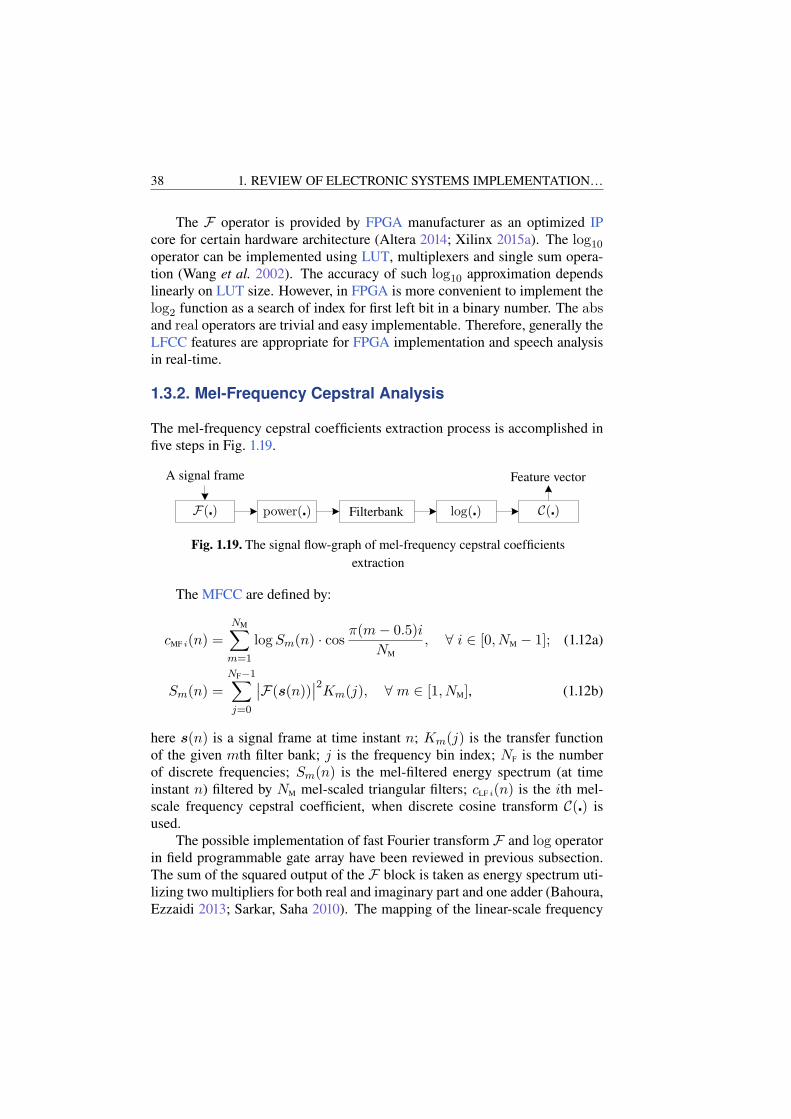
38 1. REVIEW OF ELECTRONIC SYSTEMS IMPLEMENTATION…
The F operator is provided by FPGA manufacturer as an optimized IPcore for certain hardware architecture (Altera 2014; Xilinx 2015a). The log10operator can be implemented using LUT, multiplexers and single sum opera-tion (Wang et al. 2002). The accuracy of such log10 approximation dependslinearly on LUT size. However, in FPGA is more convenient to implement thelog2 function as a search of index for first left bit in a binary number. The absand real operators are trivial and easy implementable. Therefore, generally theLFCC features are appropriate for FPGA implementation and speech analysisin real-time.
1.3.2. Mel-Frequency Cepstral Analysis
The mel-frequency cepstral coefficients extraction process is accomplished infive steps in Fig. 1.19.
A signal frame
F(�) power(�) Filterbank log(�) C(�)
Feature vector
Fig. 1.19. The signal flow-graph of mel-frequency cepstral coefficientsextraction
The MFCC are defined by:
cMF i(n) =
NM∑
m=1
logSm(n) · cosπ(m− 0.5)i
NM
, ∀ i ∈ [0, NM − 1]; (1.12a)
Sm(n) =
NF−1∑
j=0
∣∣F(s(n))∣∣2Km(j), ∀ m ∈ [1, NM], (1.12b)
here s(n) is a signal frame at time instant n; Km(j) is the transfer functionof the given mth filter bank; j is the frequency bin index; NF is the numberof discrete frequencies; Sm(n) is the mel-filtered energy spectrum (at timeinstant n) filtered by NM mel-scaled triangular filters; cLF i(n) is the ith mel-scale frequency cepstral coefficient, when discrete cosine transform C(�) isused.
The possible implementation of fast Fourier transform F and log operatorin field programmable gate array have been reviewed in previous subsection.The sum of the squared output of the F block is taken as energy spectrum uti-lizing two multipliers for both real and imaginary part and one adder (Bahoura,Ezzaidi 2013; Sarkar, Saha 2010). The mapping of the linear-scale frequency

1. REVIEW OF ELECTRONIC SYSTEMS IMPLEMENTATION… 39
to the mel-scale frequency in a filterbank block is realized according to loga-rithmic dependence:
mel(f) = 1127 ln(1 +
f
700
), (1.13)
here f is linear frequency; mel(f) is a mel-scale frequency.
Instead of implementing the (1.13) directly in a hardware, the transfer func-tion coefficients Km(j) usually are stored in read-only memory and the mel-filtered energy spectrum can by implemented on single multiply-accumulateunit (Bahoura, Ezzaidi 2013; Schmadecke, Blume 2013; Vu et al. 2010). Thefilter banks can be implemented with multiplexer, shifts and additions (Sta-worko, Rawski 2010). Thus the size of multiplexers and the number of com-binational circuits for bit shifts and additions increases proportionally to thenumber of filter coefficients. The C(�) calculation can be implemented on sin-gle MAC, where the values of the cos function are precomputed and stored inLUT (Sarkar, Saha 2010; Vu et al. 2010).
The Simulink or LabView tool can be used to fast calculation of MFCCbut such method is not always efficient due to low performance and less than100MHz of maximum operating frequency (Bahoura, Ezzaidi 2013; Farjo et
al. 2012). At least two times higher operating frequency of MFCC circuit canbe achieved using hardware description language (Veitch et al. 2010). If em-bedded processor is fast enough to calculate speech features in real-time thenit can be used in co-design with FPGA. It becomes popular and one of thefastest way to develop MFCC features extraction in FPGA with soft-core pro-cessors (Cheng et al. 2011; Manikandan, Venkataramani 2011; Pan, Li 2012;Zhang et al. 2011).
1.3.3. Linear Predictive and Linear Predictive CepstralAnalysis
Linear predictive analysis is based on simplified vocal tract model, where thevoice production can be modelled by process of passing excitation signalsthrough autoregressive filter. The coefficients of this filter describes the com-pressed voice and they are obtained by using Levinson-Durbin autoregression.The LPC features by itself are sensitive to quantization errors. Therefore, theLPC features should be converted to less quantization sensitive linear predic-tive cepstral coefficients (LPCC), which are more suitable for implementationin FPGA with fixed-point precision without (Wu et al. 2006) or with hardwareaccelerators (Liu, Bergmann 2010). These features are extracted in three steps,as is shown in Fig. 1.20.

40 1. REVIEW OF ELECTRONIC SYSTEMS IMPLEMENTATION…
A signal frame LPC vector LPCC vector
Autocorrelation Autoregression Conversion
Fig. 1.20. The signal flow-graph of linear predictive and linear predictivecepstral coefficients extraction
The autocorrelation coefficients ri are estimated by:
ri =
NW−1∑
n=0
s(n)s(n+ i), ∀ i ∈ [0,M ], (1.14)
here NW is the window length of speech signal s(n); M is the autocorrelationlength.
The systolic array is often used for autocorrelation implementation, be-cause of suitable arrangement and interconnection of DSP cores in a hardwareFig. 1.21 (Atri et al. 2012).
Signal
DSPDSPDSP
r0 r1 rM
z−1
z−1z−1
z−1
Fig. 1.21. The systolic array for the autocorrelation
The LPC and LPCC features are extracted using Levinsin-Durbin algo-rithm (Tamulevičius 2008b):
e0 = r0; k1 = r1/e; a1 = k1; (1.15)
ei =(1− k2i
)ei−1, ∀ i ∈ [1,M ]; (1.16)
ki =(ri −
i−1∑
j=1
ajri−j
)ei−1, (1.17a)
aj = aj − kiai−j , (1.17b)
cLP i = ai −i−1∑
j=1
(jicLP j ai−j
), ∀ i ∈ [1,M ] and j ∈ [1, i], (1.17c)

1. REVIEW OF ELECTRONIC SYSTEMS IMPLEMENTATION… 41
here e is the temporal energy value; k is the reflection coefficient; M is the LPanalysis order; a and cLP are the LPC and LPCC vectors.
Despite the advantage of parallelism in signal processing, the quantizationerror accumulates during the autoregression and conversion stages adverselyaffecting features accuracy (Xu et al. 2005). Therefore, the recursive part ofLPCC analysis is more often implemented on soft-core processor with floating-point arithmetic rather than pure in a hardware.
1.3.4. Features Classification
The main difficulties in speech recognition arise from speech variability, in-correct pronunciation, environmental impact, phonetic transcription similari-ties, or dictionary size limits (Tamulevičius 2008b; Čeidaitė, Telksnys 2010).Therefore, many methods for the speech features classification are developed,e.g., the dynamic time warping (DTW) (Hussain, Rashid 2012; Sart et al. 2010;Tamulevičius et al. 2010; Zhang et al. 2012), hidden Markov models (Gavat et
al. 2008; Hirsimaki, Kurimo 2004; Prochazka et al. 2011), Gaussian mixturemodels (Sojka et al. 2004) and artificial neural networks (Amudha et al. 2008).
For precise spoken word recognition with HMM it is preferred to usefloating-point numbers due to the specifics of Viterbi algorithm, which op-erates on probabilities of acoustic models. Another issue is the learning ofnew word. The phonetic transcription and the statistical model must be createdfor each new word added to dictionary. It is time consuming process. As wellas adapting the ANN, that updates the weights and changes topology, when itis trained for unknown word. Different from above mentioned classifiers, theDTW do not requires any specific training algorithm, because it needs only tostore a feature vector of new word.
We are concentrated in the speaker dependent Lithuanian isolated wordrecognition. Each spoken word can be presented as a finite set of features re-stricted in a time. The time-limited signals are most appropriate to comparewith the DTW algorithm, which is suitable for FPGA due to straightforwardarithmetic on fixed-point numbers and pipelined signal processing (Sart et al.
2010; Zhang et al. 2012). The DTW is already more than four decades oldbut still an effective method to match two templates varied in the time do-main (Ding et al. 2008). The length of each template as well as the numberof templates stored in a dictionary influences the matching time. A speed-upof the whole process can be achieved by duplication of DTW cores in singleFPGA (Hussain, Rashid 2012). Various basic and parallel DTW implementa-tions are proposed. The experimental studies in last mentioned references con-firm that using such approach one DTW can be calculated in approximately0.57ms at 100MHz clock with 64×64 size of the error matrix.
42 1. REVIEW OF ELECTRONIC SYSTEMS IMPLEMENTATION…
Another way of DTW acceleration is the normalization: reduction of thelength of all time series from their original length to the predefined length (Sartet al. 2010). This method becomes efficient when comparable data series arevery long (the duration of comparison process is proportional to the squaredlength of the time series). In a recent paper the normalization block is em-ployed to normalize the length of input series to exactly 128 samples. Theauthors claim that normalization of raw data does not affect the accuracy ofDTW. The proposed warper uses an error matrix with the 128×128 size. TheDTW is based on a systolic array that is primarily described in C language andconverted to VHDL via ROCCC compiler (Buyukkurt, Najjar 2008). The sim-ilarity search algorithm works on 250MHz clock and requires 128 clock cyclesto calculate the DTW distance. The time series with the reduced precision of8 b integers are used intentionally with the aim to increase the performance.
Even if features extraction algorithm works correct, there is still importantto chose proper classification method. The DTW method is an appropriate wayto find similarities in two vectors of features. FPGA based pipelined implemen-tation of the classification allows to accelerate speech recognition process (Pan,Li 2012; Zhang et al. 2011). A comparative study of DTW implementations ondifferent platforms shows that FPGA-based DTW outperforms the GPU andCPU-based implementations more than 44 and 2100 times accordingly (Sartet al. 2010; Zhang et al. 2012). These arguments inspires to implement DTWintellectual property core for a real-time isolated word recognition.
1.4. Conclusions of the 1st Chapter andFormulation of the Thesis Objectives
On the basis of the analytical review it is possible to assert that:
1. The higher circuit implementation level, the less guarantee that logiccircuit optimally fits to FPGA resources. However, from the designerpoint of view the system can be described faster with HLS tool.
2. The lower circuit implementation level, the more time is requited toevaluate all possible paths and find an optimal one. Lower level isdesigner unfriendly, but gives possibility to implement the circuit onan optimal criteria.
3. The FPGA contains optimized DSP, memory and logic blocks suitablefor efficient lattice-ladder multilayer perceptron (LLMLP) implemen-tation.
4. The LLMLP neural network was never before implemented on FPGA.A large number of required arithmetic resources suggests to reuse DSPslices for network implementation.

1. REVIEW OF ELECTRONIC SYSTEMS IMPLEMENTATION… 43
5. The general purpose high level synthesis tools generates design withpoor performance and are suitable only for fast concept proof, howevernot for long-term functioning solution. Therefore, specialized hard-ware description language compiler must be written for LLMLP imple-mentation with respect to hardware limitations and LLMLP specifics.
6. The trade-off between artificial neural network (ANN) accuracy, FPGAutilization rate and processing speed must be maintained, while imple-menting parallel ANN with training structures.
7. The speech signal analysis methods requires a lot of arithmetic op-erations. Some of them have recursive processes, which are not ap-propriate for implementation in a hardware. Therefore, the soft-coreprocessors must be used.
8. Using few dynamic time warping cores on single FPGA or a systolicFPGA structure it is possible to achieve fast features comparison on arelatively low system clock through increased resource utilization andpipelined design.
The following tasks must be solved:1. The creation of the technique for efficient LLMLP implementation on
FPGA based on specialized quality criteria and specifics of LLMLP.
2. Develop the optimized intellectual property (IP) cores used in Lithua-nian speech recognizer.
3. Experimentally verify the efficiency of IP cores.
4. Investigate isolated word recognition accuracy and speed.


2Efficient Implementation of
Lattice-Ladder MultilayerPerceptron
Pursuing the Task 2 of the Thesis the results of LLMLP efficient implementa-tion criteria and technique original development are presented in this chapter.In Section 2.1 LLMLP implementation quality and a set of criteria that deter-mine it are discussed. Idea of Pareto frontier calculation for the implemen-tation quality criteria is raised. A new LLMLP implementation technique isintroduced in Section 2.2. Here the specialized criteria for circuitry synthesisis brought in together with a selected way to tailor the implementation tech-nique to the intrinsic LLMLP structural features. Afterwards major stages ofthe technique are elucidated. In Section 2.3 all the steps for a single neuron pro-cessing element (NPE) optimization are in details presented. An emphasis onsubgraph matching, covering, merging and scheduling algorithms is done. Asa result the NPE is optimized for optional pipeline stages and latency/resourcesoptimal training. In Section 2.4 optimization steps of neuron layers implemen-tation are presented. Accuracy optimization as well as two equivalent imple-mentation strategies, namely throughput optimization (Subsection 2.4.2) andresource optimization (Subsection 2.4.3) are crafted by corresponding algo-rithms.
The research results are published in author publications (Sledevič, Nava-kauskas 2016, Sledevič, Navakauskas 2015, Sledevič, Navakauskas 2014). Themain results are announced in international: “Electronics” (Palanga, 2015),AIEEE (Vilnius, 2014; Riga, 2015); and national “Science – Future of Lithua-nia”(Vilnius, 2015, 2016) scientific conferences.
45

46 2. EFFICIENT IMPLEMENTATION OF LATTICE-LADDER…
2.1. Implementation Quality
As was discussed in Chapter 1, there is not enough resources for implementa-tion of large LLMLP in parallel manner even on modern FPGA. Therefore, thestrategy, that we propose to perform NPE, consists of two steps:
• implement a configurable NPE with maximal throughput maintainingshortest possible processing latency τNPE and maximal clock frequencyf⊤ of synthesized design;
• place and share the NPEs through whole LLMLP maintaining paral-lelism of synapse, neuron or layer if resources allow.
The efficient implementation of LLMLP employing multiple optimizedNPE in FPGA is a multi-criteria task dependent on the optimization goal.These criteria can split into hardware and network related groups of qualitycriteria. The amount of used resources, accuracy, power consumption andFPGA chip price are related to hardware quality criteria, which can be im-proved selecting a correct programming tool or changing FPGA chip. The sizeof LLMLP, the type of training and latency of the signal propagation from theinput layer to the output are all related to the group of network quality crite-ria improved only by the modifications in LLMLP topology. The total qualityQ covers hardware and network related criteria and is equivalent to set of allmentioned criteria:
Q = {qThr, qAcc, qRes, qCom, qPow, qPrice}, (2.1)
here qt is a quality criteria of type t: “Thr” – throughput, “Acc” – accuracy,“Res” – resource, “Com” – complexity, “Pow” – power, “Price” – price.
The performance of the NPE circuit depends on the clock frequency, whichis known only after final PAR step in the FPGA implementation chain. Usuallythe maximum clock frequency f⊤ is highly related to the coding style. Registerinsertion to the signal propagation path yields shorter delay of the signal in acritical path and higher clock frequency. Therefore, the ratio f⊤/τNPE will beused as a throughput criteria for the performance of NPE. The lower it is, theless time is needed for signal processing using single NPE. The throughput cri-teria qThr shows the maximal sampling frequency for data during the LLMLPweights updating in training mode. And in a forward filtering mode the qThrshows the maximal sampling frequency of the signals on the input of LLMLP.The qThr criteria covers the Quality of Results, processing and learning speed
criteria analysed in Section 1.2.8. The aim is to achieve lowest possible latency,which will increase the highest possible frequency for data sampling. The qThrdepends on the f⊤ at which the synthesized LLMLP can be clocked and on thelatency τNPE of signal processing by NPE:
2. EFFICIENT IMPLEMENTATION OF LATTICE-LADDER… 47
qThr = f⊤/τNPE. (2.2)
The accuracy criteria qAcc evaluates the precision of the LLMLP based onfixed-point arithmetic, since FPGA works efficiently only on integer numbers.The precision of fixed-point design must be compared with reference floating-point design implemented on PC.
qAcc ≡ Ψ (fixed-point design, floating-point design) . (2.3)
The workflow for investigation of a fixed-point design implementation is pro-posed further in this chapter.
The resources criteria qRes evaluates the equivalent amount of arithmeticRDSP, logic RLUT and memory RBRAM resources:
qRes ≡ Ψ(wserie
DSPRDSP + wserieLUTRLUT + wserie
BRAMRBRAM
), (2.4)
with respective weights wserieDSP , wserie
LUT and wserieRAM dependent on FPGA serie.
These weights are calculated when the arithmetic, logic and memory resourcesare expressed in LUT equivalent units. For 7th series Xilinx FPGA it is known
that a single DSP can be synthesized using 196 LUT, thus w(7)DSP = 196. One
BRAM contains 18432 b of with dual port access and one LUT configured to
RAM can store 32 b in this manner w(7)BRAM = 576. The LUT weight takes into
account that only 0.7–0.8 part of LUT can be efficiently utilized in FPGA dueto limited routing resources. In addition, if all the LUTs are used as RAM, then
FPGA dependent 0.3–0.5 coefficient must be applied for w(7)LUT considering that
only part of LUT can be configured as memory block.
R≡LUT ≡ RLUT + 196× RDSP + 576× RBRAM. (2.5)
The less resources is utilized, the more complex LLMLP can be implementedon FPGA. Therefore, the resource criteria is an inversion of equivalent re-sources:
qRes = 1/R≡LUT. (2.6)
The LLMLP complexity criteria qCom depends on number of layers L,neurons N , synapse order M and an optimal training algorithm from a set T:
qCom ≡ Ψ (L,N,M,T) . (2.7)
The aim is to fit largest complexity LLMLP to FPGA with minimal resource Rutilization and minimal processing latency τ optimizing by training type T:
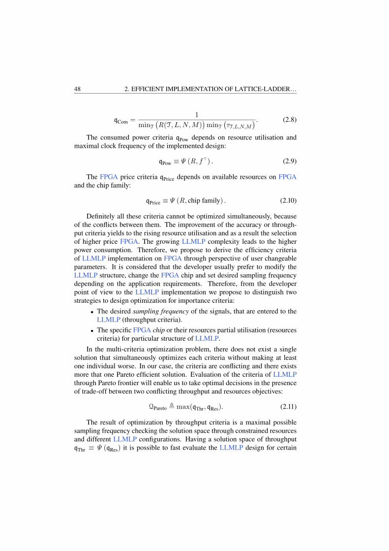
48 2. EFFICIENT IMPLEMENTATION OF LATTICE-LADDER…
qCom =1
minT(R(T, L,N,M)
)minT
(τT,L,N,M
) . (2.8)
The consumed power criteria qPow depends on resource utilisation andmaximal clock frequency of the implemented design:
qPow ≡ Ψ (R, f⊤) . (2.9)
The FPGA price criteria qPrice depends on available resources on FPGAand the chip family:
qPrice ≡ Ψ (R, chip family) . (2.10)
Definitely all these criteria cannot be optimized simultaneously, becauseof the conflicts between them. The improvement of the accuracy or through-put criteria yields to the rising resource utilisation and as a result the selectionof higher price FPGA. The growing LLMLP complexity leads to the higherpower consumption. Therefore, we propose to derive the efficiency criteriaof LLMLP implementation on FPGA through perspective of user changeableparameters. It is considered that the developer usually prefer to modify theLLMLP structure, change the FPGA chip and set desired sampling frequencydepending on the application requirements. Therefore, from the developerpoint of view to the LLMLP implementation we propose to distinguish twostrategies to design optimization for importance criteria:
• The desired sampling frequency of the signals, that are entered to theLLMLP (throughput criteria).
• The specific FPGA chip or their resources partial utilisation (resourcescriteria) for particular structure of LLMLP.
In the multi-criteria optimization problem, there does not exist a singlesolution that simultaneously optimizes each criteria without making at leastone individual worse. In our case, the criteria are conflicting and there existsmore that one Pareto efficient solution. Evaluation of the criteria of LLMLPthrough Pareto frontier will enable us to take optimal decisions in the presenceof trade-off between two conflicting throughput and resources objectives:
QPareto , max(qThr, qRes). (2.11)
The result of optimization by throughput criteria is a maximal possiblesampling frequency checking the solution space through constrained resourcesand different LLMLP configurations. Having a solution space of throughputqThr ≡ Ψ (qRes) it is possible to fast evaluate the LLMLP design for certain

2. EFFICIENT IMPLEMENTATION OF LATTICE-LADDER… 49
FPGA. During the optimization by resource criteria, the LLMLP design isoptimized for minimal resource utilisation giving as an input arguments qThrand LLMLP structure: qRes ≡ Ψ (qThr). Such approach enables us to selectthe cost efficient FPGA chip in resources utilisation Pareto optimal surface forcertain qThr criteria and net complexity. The throughput and resource optimalalgorithms for desired complexity LLMLP evaluation are elucidated in nextsubsections.
The power and price criteria are considered to be second importance, sincethe close relation with resources requirement. The suitability of certain train-ing circuit and accuracy must be investigated before the optimization by firstimportance criteria. The efficient training circuit depends only on the synapseorder, therefore the predefined optimal training type can be hardwired to the de-sired LLMLP complexity criteria qCom. The required precision for the signalsin fixed-point design will be estimated in comparison with the same floating-point design. The determined optimal width of the signals will be used in allthe prospective LLMLP implementations.
The main difference between proposed criteria for LLMLP implementa-tion and analogous purpose criteria for efficient ANN implementation is thatproposed criteria takes into account conflicting requirements as throughput andresources. While majority of analogous purpose criteria uses single-objectiveoptimization by criteria listed in Section 1.2 (Misra, Saha 2010).
2.2. Introduction to Implementation Technique
A direct implementation of LLN with its cost-effective t3 type training circuitin a hardware will require: 9M +1 multiplications for the forward LLF and itsregressor calculations. 4M +2 multiplications are required for weight updatesin (1.5) and (1.6), and 2 multiplications for δ calculation in (1.7). Thus, a hard-ware implementation of the LLN with N inputs and M th order synapses withits training algorithm in total requires N(13M + 3) + 2 multiplication opera-tions. Having N = 5 inputs and M = 3 order synapses LLN implementationwill utilize, e.g., 96% of DSP slices available in Artix-7 XC7A100T FPGA.Therefore, willing to increase the size of LLN the DSP slice resources mustbe shared. Moreover, the LLF with the regressor lattice cannot be pipelined toreceive and process data simultaneously with filter coefficients update at eachrising edge of clock, because the value of updated weight for next input sam-ple is dependent on the present value of neuron output. Therefore, the FPGAresources must be shared in time over several operations. Such approach elim-inates long idle period for single DSP slice and tends to compact all necessaryoperations for LLMLP also optimizing the total latency.
50 2. EFFICIENT IMPLEMENTATION OF LATTICE-LADDER…
All recent FPGA have dedicated DSP slices for fast arithmetic implemen-tation. Such a DSP slice can be shared to process data from different sourcesand also it can be dynamically reconfigured to implement different processingorders. The DSP block is purposely designed for pipelined data processingwith maximum performance. This is achieved inserting flip-flops and mini-mizing critical path in a circuit, as shown in Fig. 1.2. Sequentially connectedflip-flops introduce latency of 4 clock cycles in the data flow processing in-dependently on the selected instantaneous DSP configuration and subgraphconstellation (Xilinx 2014a).
The flexible structure of DSP slice (Fig. 1.2) can be considered as a con-figurable directed subgraph, where each vertex express certain arithmetic oper-ator. The source vertices are interconnected with destination vertices by edges.Each edge has a delay element consisting of D-type flip-flops, that fragments asignal-flow path of the subgraph in smallest possible pieces (operators isolatedby flip-flops) and enables the shortest propagation time of the signal betweenadjacent vertices.
The LLMLP with its training circuit contains addition, subtraction andmultiplication operations. All these operations are supported by DSP. There-fore, the LLMLP can be also successfully represented as a data flow graph(DFG), which is composed form a set of subgraphs that are supported by theDSP block. The aim is to partition whole LLMLP graph into subgraphs andthen cover the graph with largest detected subgraphs minimizing resource uti-lization. The DSP slice subgraph has maximum four input terminal vertices: A,B, C, D and a single output terminal vertex P in Fig. 1.2. The source vertex canbe connected with a destination vertex to create a subgraph only if the sourcevertex has no branches to other vertices except the unique branch to destina-tion vertex. Such a constraint follows from physical DSP slice structure. Itis reasonable to cover largest subgraphs first, as such approach decreases totalnumber of subgraphs resulting in minimal latency and reduces FPGA resourceusage, since the internal signals in DSP do not need to be stored in registersoutside DSP.
In general, each LLMLP can be described as a set (2.12) of equations. TheLLMLP implementation on FPGA is based on the translation of LLMLP equa-tions from human-readable high-level of abstraction to the low level machinecode. Such tool, which translates the high-level language into a lower-levelcode, is called a compiler. In our case the compiler takes a file with LLMLPequations and transforms it to HDL file understandable for machine in register-transfer level. The HDL file later is used in FPGA vendor tool for implemen-tation of bit file for FPGA programming.
The stages of the technique for efficient LLMLP implementation on FPGAis shown in Fig. 2.1. It is based on the conversion of LLMLP equation to the

2. EFFICIENT IMPLEMENTATION OF LATTICE-LADDER… 51
M , N , L
Equation generation
Directed data flow graph generation
Subgraph matching
Graph covering and merging
Critical path search
Resource-constrained scheduling
HDL generation
NPE optimization for optional pipeline stage
Accuracy qAcc optimization
Pareto efficient qThr, qRes optimization
LLMLPtraining
LLMLPtemplates
M , T
minR
min τ
Neu
ron
opti
miz
atio
n
Lay
erop
tim
izat
ion
NPE instructions and HDL files
Fig. 2.1. The proposed technique for lattice-ladder multilayer perceptronimplementation in field programmable gate array
DFG and splitting it to the DSP supportable subgraphs and further schedul-ing of DSP operations. At the first stage the LLMLP is expressed as set ofequations:
Seq = {eq1, eq2, . . . , eqK}. (2.12)
Each equation must have two operands and single operator (e.g., eq1 = f1 +b1). Such only two operand restriction comes from physical property for im-plementation of arithmetic operation in FPGA keeping shortest possible delayin critical path for triggered circuits. The generation of these equations is au-tomated for the LLMLP with various filter order M , number of neurons N ,layers L and training types T. The list of arbitrary operators necessary to de-scribe LLMLP is summarized in Table 2.1.
Input equations for first order direct and regressor (type t3) lattices areshown in Example 1. The equations describes a flow graph presented in Fig. 2.4.

52 2. EFFICIENT IMPLEMENTATION OF LATTICE-LADDER…
Table 2.1. The list of operators required for lattice-ladder multilayer percep-tron implementation
Operator Operator meaning
+ Addition of two signals
− Subtraction of two signals∗ Multiplication of two signals= Signal delay for single clock cycle# Read the value of activation function from LUT∼ Read the value of trigonometric function from LUT
Example 2.1 (Equations for first order direct and regressor lattices)
1) * f1c1 x c1 ; 12) + AD1 Svb0 b1v1 ;
2) * zb0s1 zb0 s1 ; 13) + N1 b1v1 LCs1 ;
3) * f1s1 x s1 ; 14) - CB1 f1v1 B1 ;
4) * zb0c1 zb0 c1 ; 15) * LCs1 LC1 s1 ;
5) - b0 f1c1 zb0s1 ; 16) - LCsAD1 AD1 LCs1 ;
6) + b1 f1s1 zb0c1 ; 17) * LCsADs1 LCsAD1 s1 ;
7) * b1v1 b1 v1 ; 18) + B1 LCsADs1 L1 ;
8) * b0v0 b0 v0 ; 19) + D0 N1 b0v0 ;
9) + Svb0 b1v1 b0v0 ; 20) * Nabla1 CB1 ncos1 ;
10) * f1v1 x v1 ; 21) = zb0 b0 b0 ;
11) + LC1 L1 f1v1 ; 22) = L1 D0 D0 ;
As it follows from analytical review of ANN implementation on FPGA theLLMLP was never before implemented on FPGA. Proposed method shares thearithmetic, memory and logic resources of FPGA in order to minimize resourceusage. The main differences between proposed and known methods for ANNimplementations on FPGA is that they do not take advantage of dynamic re-configurability of DSP and dedicate single DSP for synapse of neuron (Misra,Saha 2010). Even if the reconfigurability feature of DSP is employed, but notshared, it restricts the size of synthesized circuit (Ronak, Fahmy 2014) andtherefore the desired high complexity of LLMLP is limited.
2.3. Neuron Processing Element Optimization
2.3.1. The Data Flow Graphs Generation
At the DFG generation stage the operators in the set Seq are converted to a set ofvertices V(G) connected by set of edges E(G) in a directed graph G = (V,E)together with initial and terminal edges to vertex (E → V) maps assigning

2. EFFICIENT IMPLEMENTATION OF LATTICE-LADDER… 53
to every edge E an initial vertex init(E) and a terminal vertex ter(E). Thevertex V ∈ V represents an operator or an input port. Each operational vertexV has two inputs and attributes specifying its operator type. An edge E =(init(E), ter(E), P
)∈ E indicates a data transfer from init(E) to input port
P of ter(E).The DFG of LLMLP is stored as an adjacency list, since list is a compact
and memory efficient way for formal description of DFG instead of sparseadjacency or incidence matrices. Each row in adjacency list is related withcertain destination vertex and store a set of source vertices.
2.3.2. Subgraph Matching
On this step all the DSP supportable subgraphs GDSP described by (1.1) and il-lustrated in Fig. 2.2 must be found in a graph G. We consider that the mark +/−
denotes two different operators, then 15 types of subgraphs G(x)DSP ⊆ GDSP |x ∈
[1, 15] must be enumerated. The first subgraph G(x)DSP in Fig. 2.2 has indices
x ∈ [1, 4], the 2nd–4th subgraphs have x ∈ [5, 12] and the 5th–6th subgraphshave x ∈ [13, 15].
Through subgraphs G(x)DSP search in a graph G = (V,E), all G(x)
DSP are matched
with a subgraphs G′ = (V′,E′), where V′ ⊆ V and E′ ⊆ E. The G(x)DSP is detected
in G if there exist one-to-one correspondence between vertices of subgraphs
G(x)DSP =
(V(x)DSP,E
(x)DSP
)and G′ = (V′,E′), when G
(x)DSP contains all the edges E ∈ E′
with initial vertex init(E) ∈ V(x)DSP and terminal vertex ter(E) ∈ V
(x)DSP, then two
subgraphs G(x)DSP and G′ are equal G(x)
DSP = G′ and isomorphic. During the sub-graph matching the DSP constraints must be satisfied. Therefore, the subgraphis registered and indexed if it has only single branch between any two internalnodes. The depth-first search (DFS) strategy with respect to DSP constraintsis implemented in proposed subgraph matching Algorithm 2.1.
AAAA
BB
BB
C|P
C|PC|P
C|P DDDDD
PP
PPP
P
+/
−
+/
−
+/
−
+/
−
+/
−
+/
−
+/
− ××
××
Fig. 2.2. The subgraphs compatible with configurations of digital signalprocessing slice

54 2. EFFICIENT IMPLEMENTATION OF LATTICE-LADDER…
Algorithm 2.1 (The DFS and constraints based subgraph matching)
Require: Graphs: G = (V,E), G(x)DSP |x ∈ {1, . . . , 15}.
1: for i in 1 to |G | do
2: if ∃!x ∈ {13, 14, 15} : Vi = V xDSP,1 then
3: reg(V(x,l(x))Sg = {Vi},E
(x,l(x))Sg = 0); l(x)++.
4: if |E(Vi)| = 3 and ∃!m ∈ {1, 2, 3} : Vi = init(Em) then
5: Vj = ter(Em).6: if ∃x ∈ {5, . . . , 12} : Vj = V x
DSP,2 then
7: reg(V(x,l(x))Sg = {Vi, Vj},E
(x,l(x))Sg = {Em}); l(x)++.
8: if |E(Vj)| = 3 and ∃!n ∈ {1, 2, 3} : Vj = init(En) then
9: Vk = ter(En).
10: if ∃x ∈ {1, . . . , 4} : Vj = V(x)
DSP,3 then
11: reg(V(x,l(x))Sg = {Vi, Vj , Vk},E
(x,l(x))Sg = {Em, En});
l(x)++.12: end if
13: end if
14: end if
15: end if
16: end if
17: end for
18: return V(x,l(x))Sg ∈ V,E
(x,l(x))Sg ∈ E, l(x) |x ∈ {1, . . . , 15}.
The proposed subgraph matching algorithm return subsets of vertex V(x,l(x))Sg
and edges E(x,l(x))Sg for detected subgraphs G(x,l(x))
DSP in G and the number l(x) ofregistered subgraphs for each type of subgraph x.
2.3.3. Graph Covering and Merging
The graph G covering is a G(x)DSP selection process, that attempts to find an ap-
propriate set of subgraphs which minimizes resources usage and latency. The
largest subgraphs G(x)DSP detected in graph G are covered first using greedy al-
gorithm (Cong, Jiang 2008; Ronak, Fahmy 2014). The greedy covering algo-rithm adapted to our set of subgraphs is shown in Algorithm 2.2. It checks
presence of largest subgraphs G(x,i)Sg first in G scanning through all subgraph
types x ∈ {1, . . . , 15} and through all ith subgraphs belonging to particular
type x. The covered subgraphs are registered in G(k)C . Afterwards, all sub-
graphs G(y,j)Sg with overlapping vertices are eliminated from a set of candidates
for further covering.

2. EFFICIENT IMPLEMENTATION OF LATTICE-LADDER… 55
Algorithm 2.2 (Graph covering, subgraph elimination and merging)
Require: Graphs: G = (V,E), G(x)Sg , l(x) |x ∈ {1, . . . , 15}.
1: for x in 1 to 15 do
2: for i in 1 to l(x) do
3: if G(x,i)Sg is valid then
4: Cover G(x,i)Sg on G: G(k)
C = G(x,i)Sg , k++.
5: if ∃V(y,j)Sg ∧V
(x,i)Sg | y ∈ {1, . . . , 15}, j ∈ {1, . . . , l(y)} then
6: Eliminate candidate graph G(y,j)Sg .
7: end if
8: end if
9: end for
10: end for
11: for i in 1 to k do
12: if |V(i)C | ≥ 2 and operator of V(i)
C (|V(i)C |) is +/− then
13: if ∃!V (j) ∈ V(j)C : V j = init
(E(i)C
(V(i)C (|V(i)
C |)))
6= V(i)C (|V(i)
C | − 1)
then
14: if ∃! ter(E(V (j))
)= V
(i)C (|V(i)
C |) then
15: Merge G(i)C with G
(j)C .
16: Modify instruction and latency for G(i)C .
17: end if
18: end if
19: end if
20: end for
21: return G(x)C |x ∈ {1, . . . , k}.
The DSP has a property to add/subtract output value P of previous clockcycle through the multiplexed output feedback to last vertex of DSP subgraph,as shown in Fig. 1.2. Therefore, DSP must be reconfigured to access output Pinstead of input C (1.1). Such DSP configuration allows to process a subgraphin single clock cycle due to the pipelined subgraph processing. In order toapply the pipelining for two or more adjacent subgraphs, the pairs of subgraphsmust be merged, when a common edge exists between two terminal vertices.We distinguish few important circuits inherent for LLMLP, where subgraphmerging can be applied, as shown in Fig. 2.3. The graph for first order lattice
consists of four subgraphs as shown in Fig. 2.3a. The G(1)C is merged with
G(2)C and G
(3)C with G
(4)C . The DSP instructions for subgraphs G(2)
C and G(4)C are
modified to P = P + D × B. The graph of ladder filter (Fig. 2.3b) and sum
of synapses (Fig. 2.3c) consists of merged subgraphs G(1)C , G(2)
C and G(3)C . In a

56 2. EFFICIENT IMPLEMENTATION OF LATTICE-LADDER…
f1
b1
f0
b0
sinΘ1 sinΘ1
cosΘ1
cosΘ1
cosΘ1 f1 b0 sinΘ1
f0 b1
G(1)C
G(2)C
G(3)C
G(4)C
a)
b2 b1 b0
v2 v1 v0
sout
b2 v2 b1 v1
b0 v0
sout
G(1)C
G(2)C
G(3)C
b)
s1 s2 s3 s4
s5 s6
sout
sout
s1
...
s6
G(1)C
G(2)C
G(3)C
c)
Fig. 2.3. The covered and merged subgraphs (in grey) for a) lattice filter, b)ladder filter, c) sum of synapses
ladder graph the instructions for G(2)C and G
(3)C are modified to P = P+ D× B.
The P = P + D + A instruction is assigned to G(2)C , G(3)
C for sum of synapsesgraph. All modified instructions will be executed in single cycle. The covered
and merged subgraphs G(k)C are returned for further scheduling.
The example of first order synapse with t3 type regressor DFG and itspartitioning in subgraphs (in grey) is shown in Fig. 2.4. The merged subgraphsare connected by grey curves.
2.3.4. Critical Path Search
The scheduling is resources constrained due to limited FPGA resources forLLMLP implementation. Only single neuron with 5 inputs and 3rd ordersynapses is suitable to fit into FPGA without DSP sharing (Sledevič, Nava-kauskas 2015). Therefore, the arithmetic resources must be shared throughother operations simultaneously exploiting the pipeline property of DSP. More-over, each instruction must be exactly placed in time maintaining shortest la-
tency for whole covered graph G(x)C execution. It is known, that for resources
unconstrained scheduling the critical path method (CPM) gives a shortest pos-sible delay limited only by data dependence in critical path. For the reason that
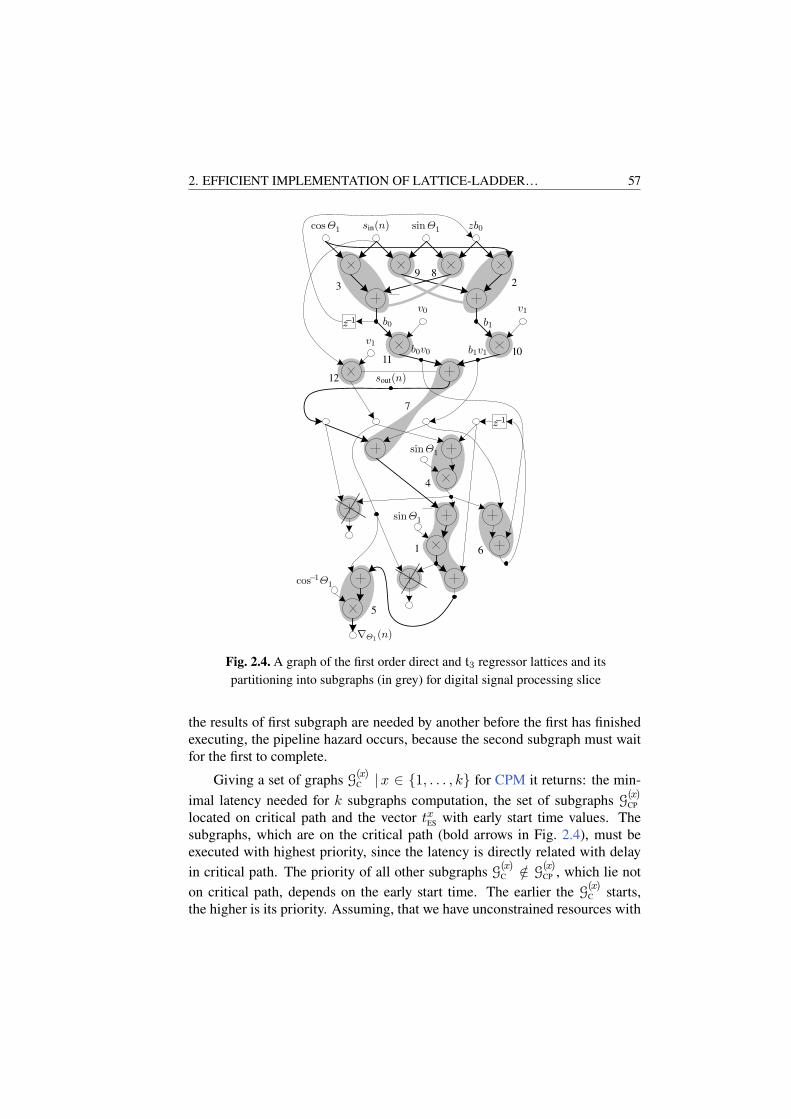
2. EFFICIENT IMPLEMENTATION OF LATTICE-LADDER… 57
cosΘ1 sin(n)
sinΘ1
sinΘ1
sinΘ1 zb0
b0
v0b1
v1
v1
b0v0 b1v1
cos−1Θ1
∇Θ1(n)
sout(n)
z−1
z−1
1
23
4
5
6
7
89
1011
12
Fig. 2.4. A graph of the first order direct and t3 regressor lattices and itspartitioning into subgraphs (in grey) for digital signal processing slice
the results of first subgraph are needed by another before the first has finishedexecuting, the pipeline hazard occurs, because the second subgraph must waitfor the first to complete.
Giving a set of graphs G(x)C |x ∈ {1, . . . , k} for CPM it returns: the min-
imal latency needed for k subgraphs computation, the set of subgraphs G(x)CP
located on critical path and the vector txES with early start time values. Thesubgraphs, which are on the critical path (bold arrows in Fig. 2.4), must beexecuted with highest priority, since the latency is directly related with delay
in critical path. The priority of all other subgraphs G(x)C /∈ G
(x)CP , which lie not
on critical path, depends on the early start time. The earlier the G(x)C starts,
the higher is its priority. Assuming, that we have unconstrained resources with

58 2. EFFICIENT IMPLEMENTATION OF LATTICE-LADDER…
unlimited interconnections, the schedule for first order synapse and its trainingcircuit is shown in Fig. 2.5. The instructions connected by arrows lie on criti-cal path. The dashed lines mark slack for instructions, which not influence thetotal latency.
2.3.5. Resource Constrained Scheduling
In a Gantt chart (Fig. 2.5) there are 12 instructions and each one requires a DSPslice to be executed. To make it implementable on single shared and pipelinedDSP, the instructions must be scheduled according to hardware constraints,maintaining shortest possible delay in critical path. The pipelined resourcescan be shared, even if the corresponding operations overlap. This necessarilyrequires that the operations do not start in the same time step and no data de-pendency exists between the operations. Moreover, the buffers are required onDSP inputs to load signals synchronously in particular time step. As a conse-quence, each instruction is lengthen by 2 clock cycles. One cycle is needed towrite result in buffer and second one to read signal from buffer.
The Gantt chart for resources constrained scheduling is shown in Fig. 2.6.
The latency of G(x)C calculation is shortest possible. It can be seen from the se-
quence of the scheduled instructions located exactly one after another in crit-ical path and connected by directed arrows. The 9th instruction starts not at0 time step, however 2 cycles later increasing total latency by 2 cycles. It isaffected by resource constraints, since only single instruction can start at each
discrete time step. The two sets of data dependent subgraphs {G(9)C ,G
(2)C ,G
(10)C }
and {G(8)C ,G
(3)C ,G
(11)C } have same 15 clock cycles latency and both belong to
0 5 10 15 20 25
8
9
12
2
3
4
10
11
6
7
1
5
i ith instruction
Slack
Clock cycles
Inst
ruct
ions
Fig. 2.5. The resources unconstrained instruction schedule for first orderlattice-ladder and regressive lattice after critical path search

2. EFFICIENT IMPLEMENTATION OF LATTICE-LADDER… 59
0 5 10 15 20 25 30 35
8
9
12
2
3
4
10
11
6
7
1
5
i
ith instruction
Clock cycles
Inst
ruct
ions
Fig. 2.6. The resource constrained schedule for first order lattice-ladder andregressive lattice graph
critical path, as shown in Fig. 2.5. Therefore, it is not important which one set
{G(9)C ,G
(2)C ,G
(10)C } or {G(8)
C ,G(3)C ,G
(11)C } starts first, since G
(10)C and G
(11)C have
same priority and both are source subgraphs for the G(7)C .
The proposed subgraph scheduling algorithm handles pipelined DSP re-sources by allowing the scheduling of overlapping operations with no datadependency and different start times. If two or more operations have samestart time, then they are delayed until DSP will be released. The stages in Al-gorithm 2.3 lines 8–14 ensure the minimal latency for instruction execution.
The algorithm includes the candidate subgraph G(x)C to set of subgraphs G
(x)L
on schedule list only if all predecessor vertices for G(x)C are computed. Then
it schedules exactly one subgraph from set G(x)L with highest priority. Thus
the subgraphs G(x)CP located on critical path are scheduled first before all other
subgraphs. The subgraphs G(x)C /∈ G
(x)CP have a slack of free time steps and are
scheduled with as soon as possible (ASAP) strategy. The algorithm returns
instruction start vector of time steps t(x)S , x ∈ {1, . . . , k}, which is used next inHDL generation placing DSP instructions in right order.
Algorithm 2.3 (Resource constrained scheduling)
Require: Graphs: G(x)C |x ∈ {1, . . . , k}, k – number of covered G
(x)C .
1: [G(x)CP , t
(x)ES , τ CP] = CPM(G(x)
C |x ∈ {1, . . . , k}).2: if ∃G(x)
CP ∧G(x)C |x ∈ {1, . . . , k} then
3: Set pri(G(x)C ) = maxx(τ
CP − t(x)ES ) for G(x)
C on critical path.4: else
5: Set pri(G(x)C ) = τ CP − t
(x)ES for all G(x)
C /∈ G(x)CP .

60 2. EFFICIENT IMPLEMENTATION OF LATTICE-LADDER…
6: end if
7: while ∃G(x)C 6= G
(x)S |x ∈ {1, . . . , k} do
8: Update predecessors ∀ V(x)C : G(x)
C = G(x)S .
9: if ∀ init(E(x)C ) predecessors are ready for E(x)
C ∈ G(x)C then
10: Add G(x)C candidates to schedule list G(x)
L = G(x)C .
11: end if
12: if ∃!G(x)L : pri(G(x)
L ) ≥ pri(G(y)L ), y ∈ {1, . . . , k} and y 6= x then
13: Schedule subgraph G(x)S = G
(x)L and remove G
(x)L form schedule list.
14: Capture instruction start time t(x)S = t.
15: if G(x)S merged with child subgraph then
16: Reserve DSP for next cycle.17: else
18: Release DSP resource.19: end if
20: end if
21: t++.22: end while
23: return t(x)S .
2.3.6. Design Description
The final architecture of processing element described in HDL is shown inFig. 2.7. It contains: single DSP as a configurable subgraph execution unit,four buffers connected to DSP inputs and the memory dedicated for nonlinearfunctions. The index generator consists of binary counter. With this counter aproper instruction is selected at each clock cycle from a set of instructions. Thesize of memory buffer depends only on the instruction width. The instructionset format consists of: four write/read addresses, DSP operation select bits,multiplexer select bits and nonlinear functions select bits in address modifica-tion block. The data buffers as well as nonlinear functions are implementedon dual (left and right) port memory. The left port of buffer is a write port,through which multiplexed data from: NPE input, result of nonlinear functionor DSP output is stored in buffers. Data are loaded to DSP through right portof buffers. The DSP output P is: returned back to buffers, connected to NPEoutput, used as argument in nonlinear activation function accessible throughleft port of dual port ROM. The sinΘj cosΘj , cos
−1Θj tables are accessedthrough the right port of ROM. Due to the additional multiplexer requirementand buffer limitation to write only single value on clock cycle, the four nonlin-ear functions are implemented on the same ROM. The access of tanh P do notneed any address modification, since the highest two bits are zeros. To accessthe sinΘj cosΘj , and cos−1Θj the address of right port is modified changing

2. EFFICIENT IMPLEMENTATION OF LATTICE-LADDER… 61
D buffer
A buffer
B buffer
C buffer
tanhP
sinΘ
cosΘ
1cosΘ
Index generator
Address modificator
Instruction generator
DSP
Operation selectInstruction bus
Input
Inputselect
Output
Dual port ROM
Dual port RAM
A
B
C
D
P
Fig. 2.7. The processing element based on single digital signal processing(DSP) slice
the highest two bits to “01”, “10”, “11” respectively in address modificationcore.
Due to the simplification the delay elements in Fig. 2.7 are marked by “|”crossing data lines. Through the read/write operation memories brings addi-tional single clock cycle latency, therefore the minimal latency of single in-struction execution is equal to seven clock cycles: one cycle to read data frombuffer, five cycles to process a certain subgraph and last one to write resultback to buffer. The two cycle latency of RAM and four cycle latency of DSPare determined by hardware constraints. The additional delay elements on eachdata line between buffers and DSP was inserted during the experimental inves-tigation of the NPE performance. The experiments were done changing thenumber of pipeline stages (delay elements) also replacing the training circuitsof LLMLP and generating the HDL file of NPE (Fig. 2.7). The timing analysisafter PAR gives the maximum clock frequency f⊤ at which the implementeddesign can run (see Table 2.2). The latency and execution time are averagedover LLF orders M = {1, . . . , 10} and four different training circuits. An in-creased number of pipeline stages results in increased f⊤, but also contributesto an increase of latency taken to complete the processing of an instruction.Therefore, the time optimal instruction execution was achieved with one addi-tional flip-flop (delay element) between flip-flops located in buffers output andDSP inputs, as shown in Table 2.2 and in Fig. 2.8.
Only the forward pass synapse and its regressor lattice is used in the in-vestigation of optional pipeline stages in the NPE, since all other particularcircuits which form LLMLP are independent on training type and are same forall the configurations of LLMLP. To identify an optimal number of optionalpipeline stages in NPE, the execution time of forward pass synapses τ s→֒
M,T,f⊤

62 2. EFFICIENT IMPLEMENTATION OF LATTICE-LADDER…
Table 2.2. Timing results of neuron processing element
Optional pipeline stages 0 1 2 3 4Average latency, cycles 613 668 728 798 869
f⊤, MHz 207 320 339 339 339Average execution time, µs 2.96 2.09 2.15 2.35 2.56
Optional pipeline stage
Rel
ativ
epr
oces
sing
tim
e
t3t4t11t12
0 1 2 3 40.6
0.65
0.7
0.75
0.8
0.85
0.9
0.95
1
Fig. 2.8. The relative processing time dependence on optional pipeline stageand training type
must be compared between order M , train type T and maximal clock frequencyf⊤ of the design. For the comparison purposes, the execution time R̄time
M,T,f⊤ isaveraged over synapse order M in (2.13) and normalized to the highest valueover four types of investigated regressors in (2.14):
R̄timeM,T,f⊤ =
1
M
M∑
m=1
τ s→֒m,T,f⊤
/f⊤, (2.13)
R̂timeM,T,f⊤ ≡ R̄
timeM,T,f⊤
/maxT
R̄timeM,T,f⊤ , (2.14)
here T – regressor type, T ∈ {t3, t4, t11, t12}; f⊤ – maximum clock frequency,
which is investigated changing the number of pipeline stage; R̂timeM,T,f⊤ – ex-
ecution time of NPE relative to highest average execution time R̄timeM,T,f⊤ over
different regressor. For all the training types T the fastest execution is achievedwith single optional pipeline stage, as shown in Fig. 2.8.
Maintaining synapse parallelism the LLN with N inputs consists of N+1NPE, as shown in Fig. 2.9. The weight updating circuit, forward and regres-sor lattice of the certain nth input is implemented on nth NPE. The additionalNPE is used for the summation of synapse outputs and instantaneous error cal-

2. EFFICIENT IMPLEMENTATION OF LATTICE-LADDER… 63
culation. To form a layer with N neuron parallelism the single neuron design(Fig. 2.9) must be implemented N times.
The scheduled list of instructions for DSP generated by our technique canalso be used in NPE created in Xilinx System Generator (XSG) tool. In thiscase, the NPE must be assembled manually in XSG by adding input buffers,memories for instructions and nonlinear functions, multiplexers and delay ele-ments to the DSP slice. After the creation of NPE (Fig. 2.7) it remains only toload four initial coefficient files for instruction indices, instructions, nonlinearfunctions and buffers.
2.4. Neuron Layers Optimization
Two strategies are proposed for neuron layers optimization. Throughput opti-mized strategy, when NPE is dedicated for each forward and backward synapseand node. The layer parallelism is reduced untill LLMLP structure fits in theconstrained FPGA resources. The resources optimized implementation stra-tegy begins from LLMLP implementation on single NPE and iteratively addsnew NPE to the design untill meets processing time requirements.
2.4.1. Accuracy Optimization
A. Bit Width Selection
The workflow for the constrained lattice-ladder neuron implementation analy-sis is shown (Fig. 2.10). Program Matlab is used to create a reference designworking on floating-point data. The essential for the investigation parametersare two K length vectors of the lower f l and the upper f h cut-off frequenciesthat determine various band-pass M th order lattice-ladder synapses. Otherinvestigation common parameters are N length input and desired output sig-
Input 1
Input 2
Input N
Output
PE1
PE2
PEN
PEN+1
Fig. 2.9. The architecture of neuron with synapse parallelism

64 2. EFFICIENT IMPLEMENTATION OF LATTICE-LADDER…
nals (sin, s⋆out) to be used for training and validation. Program Vivado HLSfrom Xilinx is used to create, simulate and analyse constrained design. Con-straint parameters: precision of fixed-point arithmetic in W bits and BRAMsize. After the simulations of floating-point and fixed-point designs the LLNparameters Θj and vj are compared to determine the bandwidth and band-passcentral frequency discrepancies.
The latency of sinΘj and cosΘj values generation on parallel CORDICcore is directly proportional to the word length used for Θj variables. There-fore, CORDIC is expensive for high accuracy. Alternative approach could beto store in memory only quarter of sine period and to generate the rest valuesby simple manipulations with values and memory addresses, i.e., interpret Θj
as an address in the LUT. During the investigation T = 16 k addresses are al-located in BRAM to form quarter of sine period (similarly for inverse cosine)and that was not changed even when word length of data was varied.
The Vivado HLS lets to create a new W = Wi + Wf length fixed-pointtypes with the desired number of bits for integer Wi and fractional Wf parts.The overflow of integer bits is avoided by enabling saturation, thus value of thesignal never exceeds the margins, e.g., [−4, 4) for Wi = 3.
The neuron training step needs to be constrained from both sides. Thelower bound of µ needs to be restricted because during weights Θj and vjupdates in (1.5) and (1.6) the product of three small parameters must be con-sidered. Therefore the precision of µδ∇Θj
(n) and µδ∇bj (n) is doubled inten-
f l, f h, M , sin, s⋆outW = {10, 12, 18, 25},
Tsin, Tcos
Reference design Constrained design
Floating-point simulation Fixed-point simulation
Bandwidth comparison
Graph plotting Resource/performance analysis
Matlab Vivado HLS
Fig. 2.10. The workflow for investigation of a fixed-point implementation oflattice-ladder linear neuron and its training circuit
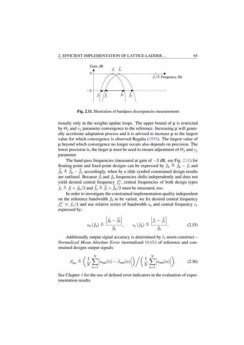
2. EFFICIENT IMPLEMENTATION OF LATTICE-LADDER… 65
Gain, dB
Frequency, Hz0
−3
fs/2
fc f̃c
fl f̃lfh f̃h
Fig. 2.11. Illustration of bandpass discrepancies measurements
tionally only in the weights update loops. The upper bound of µ is restrictedby Θj and vj parameter convergence to the reference. Increasing µ will gener-ally accelerate adaptation process and it is advised to increase µ to the largestvalue for which convergence is observed Regalia (1995). The largest value ofµ beyond which convergence no longer occurs also depends on precision. Thelower precision is, the larger µ must be used to ensure adjustment of Θj and vjparameter.
The band-pass frequencies (measured at gain of −3 dB, see Fig. 2.11) forfloating-point and fixed-point designs can be expressed by fb , fh − fl andf̃b , f̃h − f̃l, accordingly, when by a tilde symbol constrained design resultsare outlined. Because fl and fh frequencies shifts independently and does notyield desired central frequency f⋆
c , central frequencies of both design typesfc , fl + fb/2 and f̃c , f̃l + f̃b/2 must be measured, too.
In order to investigate the constrained implementation quality independenton the reference bandwidth fb to be varied, we fix desired central frequencyf⋆
c ≡ fs/4 and use relative errors of bandwidth ǫb and central frequency ǫc
expressed by:
ǫb (fb) ,
∣∣∣fb − f̃b
∣∣∣fb
, ǫc (fb) ,
∣∣∣fc − f̃c
∣∣∣fb
. (2.15)
Additionally output signal accuracy is determined by l1-norm construct –Normalized Mean Absolute Error (normalized MAE) of reference and con-strained designs output signals:
EMA ,
(1
N
N∑
n=1
∣∣∣sout(n)− s̃out(n)∣∣∣)/(
1
N
N∑
n=1
∣∣∣sout(n)∣∣∣)
. (2.16)
See Chapter 4 for the use of defined error indicators in the evaluation of exper-imentation results.

66 2. EFFICIENT IMPLEMENTATION OF LATTICE-LADDER…
B. Nonlinearity Implementation
The proposed neuron activation function is divided in three regions: pass, pro-cessing and saturation (see Fig. 2.12). In a pass region Φtanh ≡ Φident ≡ s,the signal s(n) is directly transferred to the output sout(n). The processingregion of the function Φtanh(s) is implemented in table and stored in BRAM.In a saturation region, the LLN output is always Φtanh ≡ 1.
The hyperbolic tangent function is defined as follows:
Φ̃tanh(s(n)
),
e2.03gs̄(n) − 1
e2.03gs̄(n) + 1, (2.17)
here s(n) = gs̄(n) is the input of activation function.To make the smoothed junction between the pass and processing regions,
the exponent value is set to 2.03 instead of original 2. The approximated LLNoutput can be expressed:
sout =
1, s(n) ≥ 16;
Φ̃tanh(s(n)
), 16 > s(n) > 1;
s(n), −1 ≤ s(n) ≤ 1;
−Φ̃tanh(s(n)
), −16 < s(n) < −1;
−1, s(n) ≤ 16.
(2.18)
The activation function output of negative value is obtained using asym-metry principle Φtanh
(− s(n)
)= −Φtanh
(s(n)
). The amplification coefficient
g controls the output range of the hyperbolic tangent. If g = 1, then activationfunction is linear. For g > 1, the nonlinearity in the LLN output grows. Thehigher gain is the wider range of LUT is accessible. If g = 16, then sout(n)varies in range [1, 1]. The amplification of s̄(n) more than 16 times is equiv-alent to the squeeze of activation function or similarly to increase of the slopeof hyperbolic tangent for s(n) in range [1, 1].
sout(s)
Φtanh ≡ s
0
1
45◦
1
Φtanh(s) Φtanh ≡ 1
16 s(n)
Fig. 2.12. The plot of the proposed activation function

2. EFFICIENT IMPLEMENTATION OF LATTICE-LADDER… 67
Program Matlab is used to create a reference design working on floating-point data. Program Vivado HLS is used to create, simulate and analyse con-strained design with fixed-point precision. After the simulations of floating-point and fixed-point designs, the corresponding output signals sout(n) ands̃out(n) are compared to determine the synapse transfer function and the outputsignal discrepancies.
The accuracy of the hyperbolic tangent approximation is evaluated usingl1-norm derived and commonly used indicator – Mean Absolute Error (MAE),that will depend on memory size RBRAM and gain g (Armato et al. 2011):
EMA
(g,RBRAM
),
1
n
N−1∑
n=0
∣∣∣sout(n)− s̃out
(n; g,RBRAM
)∣∣∣. (2.19)
Moreover, fixing gain to its maximum value (g = 16), the accuracy of thehyperbolic tangent approximation is also evaluated using l∞-norm – Maximum
Magnitude Error (MME), when memory size RBRAM and gain g of s(n) signalvaries (Armato et al. 2011):
EMM
(RBRAM
), max
ng=16
∣∣∣sout(n)− s̃out
(n; g,RBRAM
)∣∣∣. (2.20)
The lattice-ladder can be set to work as nonlinear low, high, band-pass orband-stop filter with additional gain control. Such a system has the transferfunction, which will have distortions dependent on the limited LUT size de-dicated to the hyperbolic tangent function. To check the accuracy of the LLNtransfer function, the LLN must be scanned by sin(n) signal, that contains allthe frequency components in range [0, fs/2], where fs is signal sampling fre-quency. The frequency of sin(n) must linearly change in time. This propertyhas the chirp signal schirp(n):
schirp(n) = cos(2πfi(n) + φ0
), (2.21)
with instantaneous frequency sweep function expressed by:
fi(n) = f0 +f1 − f0
n1n, (2.22)
here f0 and f1 are desired starting and breakpoint frequencies at time n = 0and n = n1; φ0 = 0 – signal initial phase.
To check the worst case of LLN transfer function implementation, thesynapse parameters Θm = vm ∀ m ∈ [1,M ] except v0 = 1 are set topass through all frequency components to the input of activation function.

68 2. EFFICIENT IMPLEMENTATION OF LATTICE-LADDER…
The transfer function of LLN activation function is obtained by the estima-tor (Broersen 1994):
T (f) =Pxy(f)
Pxx(f), (2.23)
here Pxy(f) – cross power spectral density of input sin(n) and output sout(n)signals; Pxx(f) – auto power spectral density of sin(n), when sin(n) ≡ schirp(n)∀ n ∈ [1, N ].
The distortions between reference and proposed LLN transfer functions areevaluated through corresponding amplitude responses by use of from l2-normderived and commonly used indicator – Root Mean Square Error (RMSE):
EAR
RMS
(g,RBRAM
),
√√√√√ 2
fs
fs/2∑
f=0
(∣∣TLNN(f ; g)∣∣−∣∣T̃LNN(f ; g,RBRAM)
∣∣)2
, (2.24)
here∣∣TLNN(f ; g)
∣∣,∣∣T̃LNN(f ; g,RBRAM)
∣∣ – floating-point and fixed-point imple-mentation LLN amplitude response with pre-selected gain g and BRAM sizeRBRAM calculated by (2.23).
2.4.2. Throughput Optimized Implementation Strategy
The total latency of the lattice-ladder multilayer perceptron training consistsof accumulated delay of the signal forward pass and error backpropagation.The latency in a forward and backward LL synapse is defined as τ →֒
T,l,M(l) andτ ←֓l,M(l) respectively. The latency in a forward and backward node is defined asτ →֒l,N(l−1) and τ ←֓
l,N(l+1) respectively. The total latency depends on the structureof the desired network. Before the optimization by latency there are knownonly the LLMLP settings: L, N (l), M (l) and the available resources R ={RDSP,RLUT,RRAM} on selected FPGA. Depending on above parameters theLLMLP is implemented through using variable degree of parallelism (Savichet al. 2012). The fully parallel design is possible only when it is enoughFPGA resources for processing signals in all synapses and nodes in paral-lel. The best performance is achieved with pipelined design and layers par-allel weight update rule when next condition is satisfied for each resource typex = {DSP,LUT,RAM}:
2L∑
l=2
(N (l−1) + 1
)N (l) < wxRx. (2.25)

2. EFFICIENT IMPLEMENTATION OF LATTICE-LADDER… 69
The latency is defined by the maximal signal delay in one of the four pipelinedstages (forward synapse, forward node, backward synapse, backward node):
τ = max2≤l≤N(L)
(minτ
(τ s→֒T,l,M(l)), τ
s←֓l,M(l) , τ
n→֒l,N(l−1) , τ
n←֓l,N(l+1)
). (2.26)
When the condition (2.25) is not meet the LLMLP is still implementedwith synapse and node parallelism, however only for single layer with maxi-mum number of synapses:
2 max2≤l≤N(L)
((N (l−1) + 1)N (l)
)< wxRx. (2.27)
Such LLMLP design is shared through all layers, therefore latency is a sumof maximum delays in forward pass or backward pass circuits over all layers:
τ =L∑
l=2
(max
(minτ
(τ s→֒T,l,M(l)) + τ n→֒
l,N(l−1) , τs←֓l,M(l) + τ n←֓
l,N(l+1)
)). (2.28)
When it is not enough resources wxRx to fit single layer of LLMLP onFPGA, the same resources are shared through forward and backward pass cir-cuits, if the next term is satisfied beginning from j = 1:
max2≤l≤N(L)
((N (l−1) + 1)N (l)
)/j < wxRx, (2.29)
here 1 ≤ j ≤ N (l⋆), when
l⋆ = argmaxl
(N (l−1)N (l)
), (2.30)
here l⋆ is a layer with maximal number of synapses.
If the design does not meet (2.29) requirement, the j will be increased untilsingle neuron fits constrained FPGA resources. On this step the synapse paral-lelism is still maintained, however the node parallelism decreases sequentiallywith rising j. For the above condition latency can be described by:
τ =L∑
l=2
(minτ
(τ s→֒T,l,M(l)), τ
n→֒l,N(l−1) , τ
s←֓l,M(l) , τ
n←֓l,N(l+1)
)j. (2.31)
And finally, if in N (l−1) layer the number of synapses exceeds the availableresources of field programmable gate array, then the synapse parallelism will

70 2. EFFICIENT IMPLEMENTATION OF LATTICE-LADDER…
be decreased with rising synapse parallelism reduction index i. The N (l−1)/i
synapses will be shared through all other synapses in N (l) layer if the term issatisfied:
max2≤l≤N(L)
(N (l−1)
/i+ 1
)< wxRx, (2.32)
here i increases in range 1 ≤ i ≤ N(argmax
l
N(l−1)). The latency of such
LLMLP can be estimated by:
τ =L∑
l=2
(imin
τ(τ s→֒
T,l,M(l)), iτn→֒l,N(l−1) , τ
s←֓l,M(l) , τ
n←֓l,N(l+1)
)N (L). (2.33)
The algorithm for throughput optimal LLMLP implementation is summa-rized in Algorithm 2.4.
Algorithm 2.4 (Throughput optimal LLMLP implementation)
Require: Load settings: L, N , M and FPGA resources Rx = {RDSP, RDSP, RDSP}.1: Compute latency matrices: τ s →֒
T,l,M(l) ,τ s←֓l,M(l) ,τ n →֒
l,N(l−1) ,τ n←֓l,N(l+1) .
2: Compute the resources utilization Rx(T, L,N,M) for fully parallel LLMLP.3: if Rx(T, L,N,M) < wxRx is true for all x then
4: Implement LLMLP with maximal performance.5: return latency τ computed by (2.26).6: end if
7: Change topology of LLMLP to single layer and compute ρ(T, L,N,M).8: if Rx(T, L,N,M) < wxRx is true for all x then
9: Implement single layer of LLMLP and share through whole net.10: return latency τ computed by (2.28).11: end if
12: Compute Rx(T, L,N,M) for single layer with shared forward/backward circuit.13: if Rx(T, L,N,M) < wxRx is true for all x then
14: Implement single layer and share it through forward/backward circuits.15: return latency τ computed by (2.31) when j = 1.16: end if
17: for j in 2 to N l⋆ do
18: Decrease node parallelism by j for single layer and compute Rx(T, L,N,M).19: if Rx(T, L,N,M) < wxRx is true for all x then
20: Implement single layer LLMLP with j reduced node parallelism.21: return latency τ computed by (2.31).22: end if
23: end for
24: for i in 1 to Nargmax
l
(N(l−1))do
25: Compute Rx(T, L,N,M) for a neuron with i reduced synapse parallelism.26: if Rx(T, L,N,M) < wxRx is true for all x then

2. EFFICIENT IMPLEMENTATION OF LATTICE-LADDER… 71
27: Implement single neuron with i reduced synapse parallelism.28: return latency τ computed by (2.33).29: end if
30: end for
31: return insufficient resources.
If the FPGA resources do not meet all the conditions: (2.25), (2.27), (2.29),(2.32), then the desired complexity LLMLP can not be implemented on theverified FPGA. This problem can be solved with the simplification of LLMLPstructure or switching to resource-rich FPGA.
2.4.3. Resource Optimized Implementation Strategy
In this case, the required latency τ req is given together with LLMLP settings:L,N (l),M (l). According to above parameters the LLMLP is implemented withminimal resources. The new processing element NPE is sequentially added tothe design, until the latency condition will be satisfied. The whole LLMLP fitsto single NPE if the next requirement is meet for i = j = k = 1:
L∑
l=2
(((minτ
(τ s→֒T,l,M(l)) + τ s←֓
l,M(l)
)N (l−1)
/i+
+(τ n→֒l,N(l−1) + τ n←֓
l,N(l+1)
))N (l)
/j
)< τ req,
(2.34)
here 1 ≤ i ≤ N l⋆−1 is the number of synapses in layer l⋆ − 1 covered byNPEs; 1 ≤ j ≤ N l⋆ is the number of neurons in layer l⋆ covered by NPEs. Thesynapse and node parallelism grows with the increasing i and j accordingly.The number of NPEs is:
RPE = (i+ 1)jk, (2.35)
here k shows how the forward and backward (fw/bf) pass circuits are imple-mented: on the same NPE (k = 1) or on different NPE (k = 2). When ondifferent NPE, then latency is defined by maximal delay in forward or back-ward pass and it must meet the conditions:
L∑
l=2
(max
(minτ
(τ s→֒T,l,M(l)) + τ n→֒
l,N(l−1) , τs←֓l,M(l) + τ n←֓
l,N(l+1)
))< τ req. (2.36)
If the above requirements are still not satisfied, then all the layers of lattice-ladder multilayer perceptron are implemented in parallel. Therefore, the la-

72 2. EFFICIENT IMPLEMENTATION OF LATTICE-LADDER…
tency, defined by the maximal signal delay in one of the four pipelined stages,must be less than required latency:
max2≤l≤N(L)
(minτ
(τ s→֒T,l,M(l)), τ
s←֓l,M(l) , τ
n→֒l,N(l−1) , τ
n←֓l,N(l+1)
)< τ req. (2.37)
The number of NPE for pipelined LLMLP implementation is:
RPE = 2L∑
l=2
(N (l−1) + 1
)N (l). (2.38)
The algorithm for resource optimal LLMLP implementation is summa-rized in Algorithm 2.5.
Algorithm 2.5 (Resource optimal LLMLP implementation)
Require: Load settings: L, N , M and required latency τ req.1: Compute latency matrices: τ s →֒
T,l,M(l) ,τ s←֓l,M(l) ,τ n →֒
l,N(l−1) ,τ n←֓l,N(l+1) .
2: Check single layer with i synapse, j node parallelism and shared fw/bw circuits:3: for j in 1 to N l⋆ do
4: for i in 1 to N l⋆−1 do
5: Compute R(T, L,N,M) for a neuron with i reduced synapse parallelism.6: if (2.34) is true then
7: Implement the LLMLP on j(i+ 1) NPEs.8: Calculate resources R(T, L,N,M).9: return R(T, L,N,M).
10: end if
11: end for
12: end for
13: Check fully parallel layer with separate circuits for forward and backward pass:14: if (2.36) is true then
15: Implement shared layer on 2N l⋆(N l⋆ + 1) NPEs.16: Calculate resources R(T, L,N,M).17: return R(T, L,N,M).18: end if
19: Check fully parallel LLMLP:20: if (2.37) is true then
21: Implement LLMLP on 2L∑
l=2
(N (l−1) + 1
)N (l) NPEs.
22: Calculate resources R(T, L,N,M).23: return R(T, L,N,M).24: end if
25: return τ req is too low.

2. EFFICIENT IMPLEMENTATION OF LATTICE-LADDER… 73
The desired complexity LLMLP can not be implemented on FPGA if therequired latency τ req do not meet all (2.34), (2.36), (2.37) conditions.
2.5. Conclusions of the 2nd Chapter
1. The technique for lattice-ladder multilayer perceptron (LLMLP) effi-cient implementation in FPGA is created and experimentally affirmedthat structure of proposed neuron processing element is speed optimalwith only 7 clock cycle latency.
2. The application of proposed lattice-ladder specific subgraph matching,covering, merging and scheduling algorithms ensures latency efficientschedule of the generated instructions for DSP, keeping the maximalclock frequency of neuron processing element IP core at 320MHz.
3. Pareto frontiers estimation for the LLMLP specialized criteria of cir-cuitry synthesis is proposed. Two implementation strategies: through-put or resources optimization, are developed and enable us to makean optimal choice of FPGA chip according to given requirements forLLMLP structure, sampling frequency and FPGA resources.
4. The work-flow for investigation of the constrained design precisionbased on band-pass discrepancies measurement is developed, ensur-ing a balance between normalized bandwidth of the synapse and theycentral frequency, bandwidth and output signal mean error.
5. The nonlinearity implementation criteria based on the evaluation ofdistortions in transfer function of lattice-ladder neuron enables us tomake and efficient choice of memory size as a trade off between theerror of proposed activation function, gain and block RAM size.


3Implementation of Lithuanian
Speech Recognizer in FieldProgrammable Gate Array
Fulfilling the Task 3 of the Thesis the results of a novel Lithuanian speechrecognizer (LSR) for disabled persons development and implementation onFPGA are presented in this chapter. A general block diagram of LSR for dis-abled persons and its final assemblage are commented in Section 3.1. Thendeveloped FPGA IP cores for speech feature extraction (Section 3.2) and wordrecognition (Section 3.3) are analyzed. Previously introduced original tech-nique for efficient implementation of LLMLP (Section 2.2), here is used forspeech filtering and noise reduction FPGA IP core development. Moreovera new accelerated pattern matching technique to speed up the word recogni-tion process using constrained dynamic time warping (DTW) is proposed. Anoriginal the double random seed matching Algorithm 3.1 is developed and pro-grammed in FPGA IP core. Lastly in Section 3.4 the original iterative voiceresponse interface enabling computer guided dialog for communication withdisabled persons is briefly described.
The research results are published in author publications (Tamulevičiuset al. 2015, Serackis et al. 2014, Tamulevičius et al. 2014, Sledevič et al. 2013,Stašionis, Sledevič 2013, Serackis et al. 2013, Sledevič, Navakauskas 2013).The main results are announced in international: “Electronics” (Palanga, 2014,2013), DAMSS (Druskininkai, 2014), ICISVC (Paris, 2014), EMS (Manch-ester, 2013), EUROCON (Zagreb, 2013); and national: “Science – Future ofLithuania” (Vilnius, 2013), “Multidisciplinary Research in Natural and Tech-nology Sciences" (Vilnius, 2014) scientific conferences.
75

76 3. IMPLEMENTATION OF LITHUANIAN SPEECH RECOGNIZER…
3.1. Speech Recognition System Overview
Whole recognition system is implemented in single FPGA chip. The wordrecognition algorithm consists of several steps, as shown in Fig. 1.17. Thespeech preprocessing involves filtering, framing and windowing. The extractedfeatures are stored in the dictionary and the spoken word is compared with apart of context dictionary. The developed IP cores are used for all features ex-traction and comparison algorithms. The hardware part of the proposed system(Fig. 3.1) is clocked at 50MHz while software part – at 100MHz.
Fig. 3.1. Illustration of six prototypes of speech recognizers (primaryversions are on the top, final version is on the bottom)
The proposed system can work in non-real-time and real-time word recog-nition modes. In the first mode, speech signal is read from external SD cardmemory for the record dataset recognition accuracy verification. In the secondmode, the speech signal is constantly captured from microphone for devicecontrol. Each implemented IP core must meet the 11.61ms delay condition inorder to work in real-time. Such requirement is defined by the 23.22ms du-ration of signal frame. Due to the half overlapping frames the time betweenincoming frames is twice shorter.
The block diagram in Fig. 3.2 shows the connectivity between IP coreswith bus width information. Each IP core in the proposed system works in-dependently and communicates with others via synchronization signals. Thesynchronization, clock and reset signals are not shown in Fig. 3.2. The audiochip is configured to sample data at 44.100 kHz. The filtering IP core involves
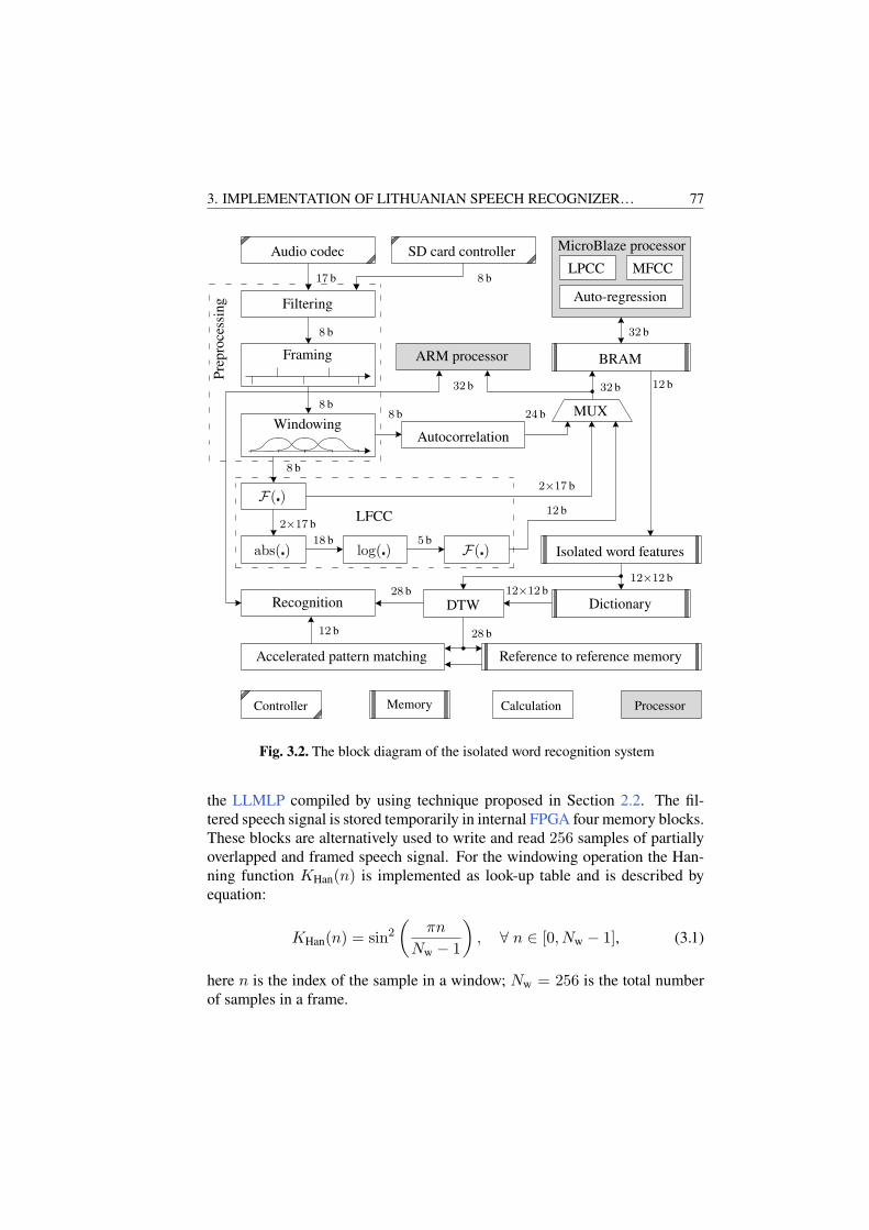
3. IMPLEMENTATION OF LITHUANIAN SPEECH RECOGNIZER… 77
8 b
8 b
8 b
8 b
8 b
12 b
12 b
12 b
17 b
28 b
28 b
32 b
32 b
32 b
12×12 b12×12 b
2×17 b
2×17 b
24 b
18 b 5 b
Controller Memory Calculation Processor
Audio codec SD card controller
Filtering
Framing
Windowing
F(�)
F(�)
abs(�)
Recognition
Autocorrelation
DTW
MicroBlaze processor
LPCC MFCC
Auto-regression
BRAM
Isolated word features
Dictionary
log(�)
LFCC
Pre
proc
essi
ng
Reference to reference memoryAccelerated pattern matching
ARM processor
MUX
Fig. 3.2. The block diagram of the isolated word recognition system
the LLMLP compiled by using technique proposed in Section 2.2. The fil-tered speech signal is stored temporarily in internal FPGA four memory blocks.These blocks are alternatively used to write and read 256 samples of partiallyoverlapped and framed speech signal. For the windowing operation the Han-ning function KHan(n) is implemented as look-up table and is described byequation:
KHan(n) = sin2(
πn
Nw − 1
), ∀ n ∈ [0, Nw − 1], (3.1)
here n is the index of the sample in a window; Nw = 256 is the total numberof samples in a frame.

78 3. IMPLEMENTATION OF LITHUANIAN SPEECH RECOGNIZER…
The soft-core processor (grey block in Fig. 3.2) is used for the IP cores thatrequire precision and operation on floating-point numbers. The decision makeris a linear function that sequentially compares two time series and matcheserrors given from DTW IP core. In the real-time mode system firstly looksfor activation word. If this word is recognized, then second spoken commandis compared with dictionary in a features space. Up to 8 copies of utterancecan be assigned to a single command to improve recognition rate. There arereserved 214 samples for each isolated word regardless of its real length. Eachword has 128 features vectors. Therefore, the size of DTW matrix is alwayspermanent and equal to 128×128. The control signal is transmitted to device,when associated command is recognized correctly.
The isolated word recognition process consists of two main parts. Firstone is the features extraction in speech signal. Second one is the comparisonof feature vectors of the just spoken word with the set of command storedin dictionary. Therefore, in the next sections the implementation of speechanalysis and comparison methods are presented.
3.2. Features Extraction Implementations
Four features extraction methods (LFCC, MFCC, LPC, LPCC) (cf. Section 1.3)are selected for speech signal analysis with the aim of future evaluation and se-lection of the best one in final application. The LFCC analysis is implementedin FPGA logic. The other analysis methods are partially implemented in FPGAand in general purpose soft-core processor, because of the requirements forfloat-point arithmetic.
3.2.1. Linear Frequency Cepstral Analysis IntellectualProperty Core
The LFCC is performed by (1.11). The hardware implementation of LFCCconsists of two fast Fourier transforms, single logarithm and abs(�) IP cores.After the windowing 8 b and 256 sample length speech signal is passed to theF(�) core. The F(�) core utilizes 3 BRAMs and 3 DSP slices. The lengthof F(�) is equal to the framed signal length. F(�) is implemented using theRadix-2 butterfly core from the Xilinx IP core generator. The latency of F(�)computation is 1662 clock cycles. The F(�) core outputs 17 b width real andimaginary spectrum series. In the abs core the absolute 18 b value is calcu-lated and sent to the log(�) core. Because the radix of a logarithm is equalto 2, this operation can be implemented in the hardware as the search for thehighest bit in data (see Fig. 3.3). The experimental verification confirms that

3. IMPLEMENTATION OF LITHUANIAN SPEECH RECOGNIZER… 79
the maximum spectrum value is never higher than 16 b. Therefore, the resultof a logarithm is in the range from 0 to 15 b and the output is described onlyby 4 b. The result is rounded to the lowest integer number.
0000001101001011. . .
000000000111011000000111101010110001010101111010
. . .
... ...
abs(�) core
Highest bit finder FFT core
256 samples
912
10
6
Fig. 3.3. Illustration of the fast log2 operator implementation
The 4 b width logarithm of the spectrum is forwarded to the next F(�) corethat calculates 12 b width LFCC features. Only real part of LFCC is saved inmemory dedicated for one word features that utilizes one BRAM. In order tocollect one word features the LFCC calculation is repeated 128 times. Thatends the LFCC feature extraction.
The LFCC calculation algorithm is sequential and there is no need to par-allelise it because one feature extraction module can be successfully sharedbetween overlapped frames and used at the end of the frame only. The abs(�)and log(�) operators are applied immediately for the complex spectrum thatcomes from the F(�) core. The second F(�) operation gives 256 cepstrum co-efficients for the one frame speech signal. Only first 12 coefficients are used infurther DTW calculation.
3.2.2. Mel-Frequency Cepstral Analysis Intellectual PropertyCore
The signal-flow graph of MFCC extraction was presented in Fig. 1.19 and de-scribed by (1.12)–(1.13). The same F(�) core, previously used in LFCC, isshared with MFCC implementation, as is shown in Fig. 3.2. The power(�) op-eration of the spectrum utilises single DSP and the result of power
(F(�)
)is
transfered to processor through shared BRAM. The multiplication with transferfunction of the filter bank (1.13), log(�) and discrete cosine transform C(�) coresare implemented on the soft-core processor due to the precision requirementsfor trigonometric, logarithmic and division operations (1.12a). The calculatedMFCC are returned back through the shared BRAM to the single isolated wordfeatures memory.
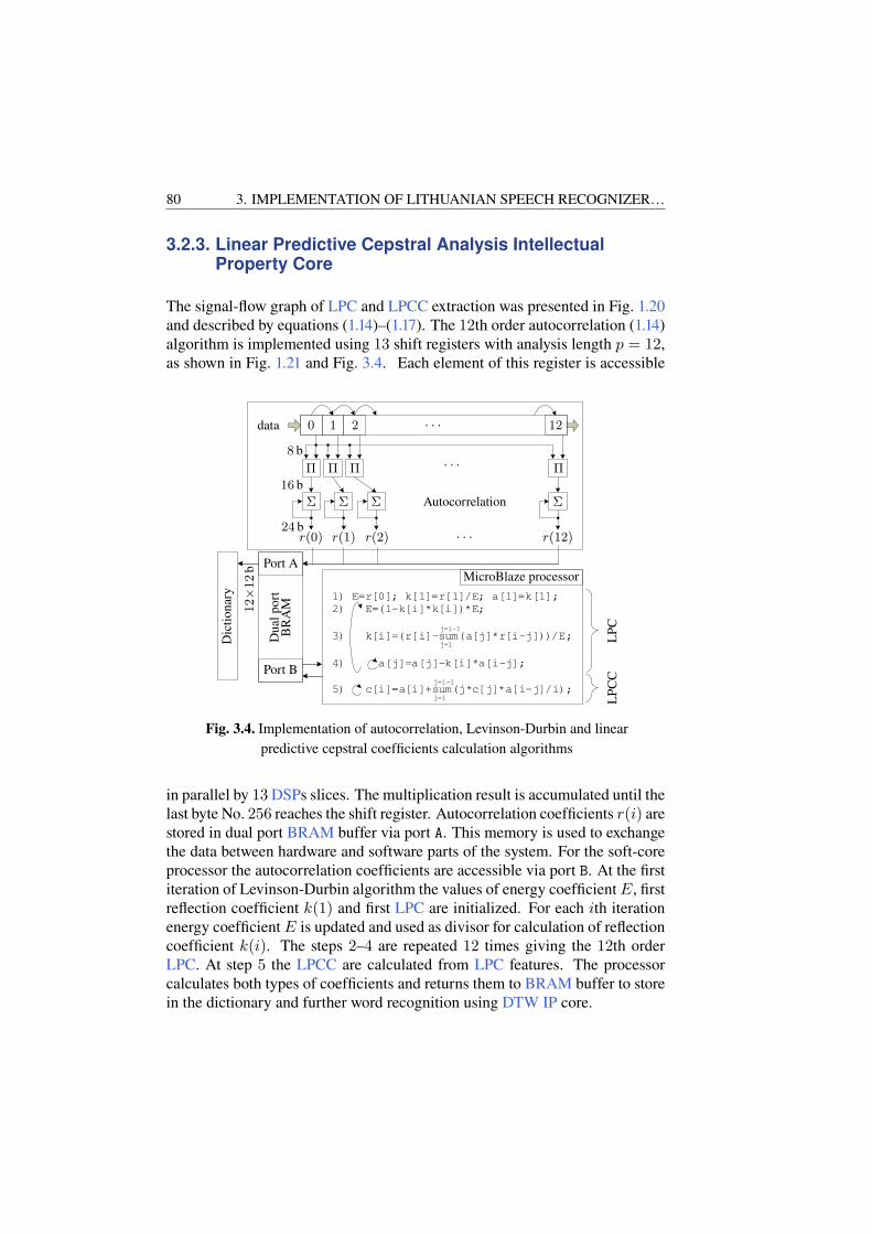
80 3. IMPLEMENTATION OF LITHUANIAN SPEECH RECOGNIZER…
3.2.3. Linear Predictive Cepstral Analysis IntellectualProperty Core
The signal-flow graph of LPC and LPCC extraction was presented in Fig. 1.20and described by equations (1.14)–(1.17). The 12th order autocorrelation (1.14)algorithm is implemented using 13 shift registers with analysis length p = 12,as shown in Fig. 1.21 and Fig. 3.4. Each element of this register is accessible
. . .
. . .
. . .
j=1
j=i-1
1) E=r[0]; k[1]=r[1]/E; a[1]=k[1];
2) E=(1-k[i]*k[i])*E;
3) k[i]=(r[i]-sum(a[j]*r[i-j]))/E;
4) a[j]=a[j]-k[i]*a[i-j];
5) c[i]=a[i]+sum(j*c[j]*a[i-j]/i);
j=1
j=i-1
data 0 1 2 12
ΠΠΠΠ
Σ ΣΣΣ Autocorrelation
8 b
16 b
24 br(0) r(1) r(2) r(12)
12×12
b
Dic
tion
ary
Port A
Port B
Dua
lpor
tB
RA
M
MicroBlaze processor
LP
CL
PC
C
Fig. 3.4. Implementation of autocorrelation, Levinson-Durbin and linearpredictive cepstral coefficients calculation algorithms
in parallel by 13 DSPs slices. The multiplication result is accumulated until thelast byte No. 256 reaches the shift register. Autocorrelation coefficients r(i) arestored in dual port BRAM buffer via port A. This memory is used to exchangethe data between hardware and software parts of the system. For the soft-coreprocessor the autocorrelation coefficients are accessible via port B. At the firstiteration of Levinson-Durbin algorithm the values of energy coefficient E, firstreflection coefficient k(1) and first LPC are initialized. For each ith iterationenergy coefficient E is updated and used as divisor for calculation of reflectioncoefficient k(i). The steps 2–4 are repeated 12 times giving the 12th orderLPC. At step 5 the LPCC are calculated from LPC features. The processorcalculates both types of coefficients and returns them to BRAM buffer to storein the dictionary and further word recognition using DTW IP core.
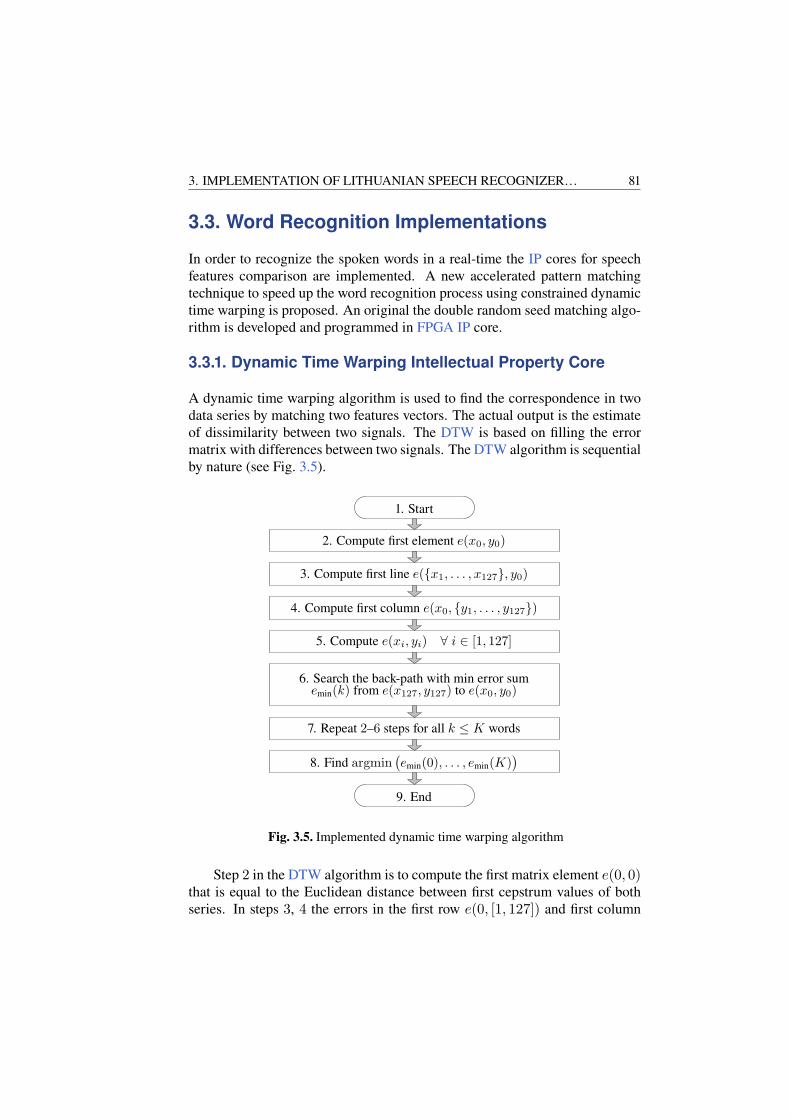
3. IMPLEMENTATION OF LITHUANIAN SPEECH RECOGNIZER… 81
3.3. Word Recognition Implementations
In order to recognize the spoken words in a real-time the IP cores for speechfeatures comparison are implemented. A new accelerated pattern matchingtechnique to speed up the word recognition process using constrained dynamictime warping is proposed. An original the double random seed matching algo-rithm is developed and programmed in FPGA IP core.
3.3.1. Dynamic Time Warping Intellectual Property Core
A dynamic time warping algorithm is used to find the correspondence in twodata series by matching two features vectors. The actual output is the estimateof dissimilarity between two signals. The DTW is based on filling the errormatrix with differences between two signals. The DTW algorithm is sequentialby nature (see Fig. 3.5).
1. Start
2. Compute first element e(x0, y0)
3. Compute first line e({x1, . . . , x127}, y0)
4. Compute first column e(x0, {y1, . . . , y127})
5. Compute e(xi, yi) ∀ i ∈ [1, 127]
6. Search the back-path with min error sumemin(k) from e(x127, y127) to e(x0, y0)
8. Find argmin(emin(0), . . . , emin(K)
)
9. End
7. Repeat 2–6 steps for all k ≤ K words
Fig. 3.5. Implemented dynamic time warping algorithm
Step 2 in the DTW algorithm is to compute the first matrix element e(0, 0)that is equal to the Euclidean distance between first cepstrum values of bothseries. In steps 3, 4 the errors in the first row e(0, [1, 127]) and first column
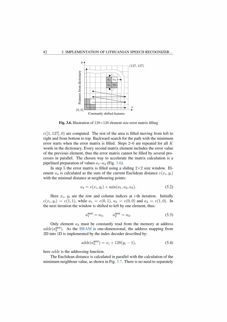
82 3. IMPLEMENTATION OF LITHUANIAN SPEECH RECOGNIZER…
Constantly shifted features
Feat
ures
from
dict
iona
ry
(0, 0)
(127, 127)
a1 a4
a2 a3
x
y
Fig. 3.6. Illustration of 128×128 element size error matrix filling
e([1, 127], 0) are computed. The rest of the area is filled moving from left toright and from bottom to top. Backward search for the path with the minimumerror starts when the error matrix is filled. Steps 2–6 are repeated for all Kwords in the dictionary. Every second matrix element includes the error valueof the previous element, thus the error matrix cannot be filled by several pro-cesses in parallel. The chosen way to accelerate the matrix calculation is apipelined preparation of values a1–a4 (Fig. 3.6).
In step 5 the error matrix is filled using a sliding 2×2 size window. El-ement a4 is calculated as the sum of the current Euclidean distance e(xi, yi)with the minimal distance at neighbouring points:
a4 = e(xi, yi) + min(a1, a2, a3). (3.2)
Here xi, yi are the row and column indices at i-th iteration. Initiallye(xi, yi) = e(1, 1), while a1 = e(0, 1), a2 = e(0, 0) and a3 = e(1, 0). Inthe next iteration the window is shifted to left by one element, thus:
anext1 = a4, anext
2 = a3. (3.3)
Only element a3 must be constantly read from the memory at addressaddr(anext
3 ). As the BRAM is one-dimensional, the address mapping from2D into 1D is implemented by the index decoder described by:
addr(anext3 ) = xi + 128(yi − 1), (3.4)
here addr is the addressing function.The Euclidean distance is calculated in parallel with the calculation of the
minimum neighbour value, as shown in Fig. 3.7. There is no need to separately

3. IMPLEMENTATION OF LITHUANIAN SPEECH RECOGNIZER… 83
compute and fill the Euclidean distance matrix, because of pipelined imple-mentation. The error matrix memory is implemented on the dual port BRAMmemory. In one clock cycle this memory is accessed twice: while readingnew a3 and writing calculated a4 value. One DTW calculation (including abackward search) needs 16 640 clock cycles to make one comparison.
. . .
. . .
Features from dictionary
One word features
Error matrix128×128×20 b
−−−−
ΠΠΠΠ
Σ
Σ
ΣΣ
ΣΣΣz−1z−1
a1 a3 a2
min
a4 e(xi, yi)sqrt
12 b
12 b
24 b
cdicti
cwordi
Fig. 3.7. Implementation of Euclidean distance and error matrix filling
The block diagram in Fig. 3.7 presents fast Euclidean distance estimationusing 11 additions, 12 subtractions, 12 multipliers and one square root core.The square root core has pipelined implementation. The calculation of Eu-clidean distance e(xi, yi) is done per one clock cycle. The difference betweenvectors is estimated by:
e(xi, yi) =
√√√√12∑
j=1
(cwordi (j)− cdict
i (j))2
, (3.5)
here e(xi, yi) – Euclidean distance between two vectors cdicti and cword
i ; cwordi (j) –
jth feature index of ith feature vector in one word feature memory; cdicti (j) –
jth feature index of ith feature vector stored in dictionary.To ensure synchronous filling of error matrix the data from dictionary, one
word buffer and error matrix are read out in parallel. Because the BRAMmemory has one clock latency for data read, therefore the valid address mustbe prepared before accessing the data. Therefore the address counter is imple-mented as separate process independent of the error calculation process. Thesetwo address and error estimation processes run synchronous. The advantage ofhardware implementation is the pipelined calculation of error matrix. At each

84 3. IMPLEMENTATION OF LITHUANIAN SPEECH RECOGNIZER…
rising edge of clock new error e(xi, yi) value is calculated and stored in errormatrix memory immediately.
0 0
20
40
60
80
10010050 50
31% 31%38%
Err
or
Features from dictionary Constantly shifted features
Fig. 3.8. The surface of the dynamic time warping error matrix withconstrained area outlined
In step 6 the use of border constraints additionally accelerates the DTWc
algorithm up to 2.6 times without a negative influence on the recognition ac-curacy. Only 38% of the total matrix area is used (see Fig. 3.8). The errorvalues near the corners are always higher than in the central part of the matrix.Therefore, the back path never comes upwards and 62% of the matrix area canbe ignored. The minimal value of the error path is iteratively calculated usingthe same 2×2 size sliding window by:
enextmin = emin +min(a1, a2, a3). (3.6)
Initially emin = e(127, 127), a1 = e(126, 127), a2 = e(126, 126) anda3 = e(127, 126). At the next rising edge of clock the sliding window isshifted to the element with the lowest error at address described by:
(xi, yi) = addr(min(a1, a2, a3)
). (3.7)
That corresponds to the following updates:
anext1 = e(xi − 1, yi), (3.8)
anext2 = e(xi − 1, yi − 1),
anext3 = e(xi, yi − 1).

3. IMPLEMENTATION OF LITHUANIAN SPEECH RECOGNIZER… 85
The minimal error path emin is computed until (xi, yi) arrives at (0, 0)location. The steps 2–6 are repeated K times, where K is the number of wordsin context dictionary. And finally, in step 7 the calculated argument of theminimal error emin(k) shows the index of recognized word.
A single DTWc core is able to compare maximum 90 word features in11.61ms (at 7800words/s) satisfying real-time requirements. To check a partof context dictionary larger than 90 words, there is proposed accelerated pat-tern matching below.
3.3.2. Accelerated Pattern Matching Intellectual PropertyCore
The idea of pattern match search acceleration is based on the assumption thatthe difference between pattern to be recognised and the reference, given indictionary is close to the difference of reference, selected for matching and ref-erence that should be found. In case this pattern matching technique is used forisolated Lithuanian word recognition, the matching error between the patternextracted for word “traukti" and randomly selected reference “augti" should beclose to the matching error between reference word “augti" and reference word“traukti", stored in the dictionary.
In order to apply given idea, the differences between references inside dic-tionary should be estimated. The differences are estimated using DTW based
0 20 40 60 80 100
4
4.5
5
5.5
6
6.5
7
×104
Reference No. 6Reference No. 12
Reference number
e min
Fig. 3.9. Reference-to-reference error distribution, calculated for tworeferences

86 3. IMPLEMENTATION OF LITHUANIAN SPEECH RECOGNIZER…
48 47 51 44 83 49 59 73 40 75 94 1 38 43 97 48 87 81 86 26 78 99 19 56
4
4.2
4.4
4.6
4.8
5×10⁴
Reference No. 6Reference No. 12
Reference number
e min
Fig. 3.10. Comparison of the 12 neighbouring reference numberdistribution for two references
algorithm. The estimation results are added to each word as a (N − 1)×2 sizematrix Mi, where N is the number of references stored in dictionary. This isa connection of two unique vectors: one with calculated reference-to-referencematching errors for each ri, where i = 1, 2, . . . , N and another – constructedfrom reference indices, corresponding to calculated matching errors.
The sorting of calculated reference-to-reference matching errors in ascend-ing order indicates references, which has similar distance (calculated usingDTW based algorithm) to analysed reference ri. Fig. 3.9 shows the compari-son of reference-to-reference distance estimation results for two references.
As it is seen in Fig. 3.9 for 6th reference we may find several references indatabase that are more similar to this reference than others – the error increaseswith noticed nonlinearity (Fig. 3.10). These references are potential causes ofpattern recognition failures. In order to reduce the risk of pattern recognitionfailure, the DTW matching is calculated between pattern p and a set of refer-ences, situated in the reference-to-reference matching vector neighborhood.
An example of reference-to-reference error matrix for 100 references isshown in Fig. 3.11. As it is seen in the figure, the reference-to-reference errormatrix is symmetrical. Taking into account this feature we may reduce theamount of additional data to store in the dictionary. However, in that case thesorting of the values will require additional algorithm to be applied.
The pattern recognition algorithm is presented in Algorithm 3.1.
Algorithm 3.1 (The double random seed matching algorithm)
Require: Load feature vectors.1: A. Random selection of initial reference ri, here i is the index of reference in
non-sorted dictionary set C.2: B. Compute the DTW matching error ep,ri for pattern p and initial reference ri.3: while Indicator of match M = 0 do
4: 1. Select n references rh = {rj+1, rj+2, . . . , rj+n}, for j = i, having reference-

3. IMPLEMENTATION OF LITHUANIAN SPEECH RECOGNIZER… 87
to-reference matching error eri,r∈Cihigher than estimated ep,ri .
5: for j = 1 : n do
6: Compute the DTW matching error ep,rj+indx.
7: end for
8: 2. Select m references rl = {rj−1, rj−2, . . . , rj−m}, for j = i, having intra-dictionary matching error era,r∈Ci
lower than estimated ep,ri .9: for indx = 1 : m do
10: Compute the DTW matching error ep,rj−indx.
11: end for
12: 3. Find the minimum matching error:emin = min{ep,rj−m
, ep,rj−m+1, . . . , ep,rj+n
};13: if emin = ep,ri then
14: ri is set as a matched reference to pattern p. M = 1.15: else
16: A new initial reference is selected ri at point with minimal error emin.17: end if
18: end while
19: C. Selection of the second reference ra.20: D. Compute the DTW matching error ep,a.21: while Indicator of match M = 0 do
22: 1. Select n references rh = {rj+1, rj+2, . . . , rj+n}, for j = a, having intra-dictionary matching error era,r∈Ci
higher than estimated ep,ra .23: for j = 1 : n do
24: Compute the DTW matching error ep,rj+indx.
25: end for
26: 2. Select m references rl = {rj−1, rj−2, . . . , rj−m}, for j = a, having intra-dictionary matching error era,r∈Ci
lower than estimated ep,ra .27: for j = 1 : m do
28: Compute the DTW matching error ep,rj−indx.
29: end for
30: 3. Find the minimum matching error:emin = min{ep,rj−m
, ep,rj−m+1, . . . , ep,rj+n
}.31: if emin = ep,ra then
32: ra is set as a matched reference to pattern p. M = 1.33: else
34: A new initial reference is selected ra at point with minimal error emin.35: end if
36: end while
37: E. Select pattern match with lower error: min{ri, ra}.
Taking into account that reference stored in the dictionary has (W/2)×Ocoefficients (here W is the width of the signal analysis window used for pa-rameter estimation; O is the analysis order), adding additional matrix Mi toeach reference will increase the dictionary by (N − 1)×2 values. It can beestimated by using the following equation:

88 3. IMPLEMENTATION OF LITHUANIAN SPEECH RECOGNIZER…
0 10 20 30 40 50 60 70 80 90 1000
10
20
30
40
50
60
70
80
90
100
Reference Number
Refe
rence N
um
ber
1
2
3
4
5
6
7
8
ra
ra
ri
ri
×104
Fig. 3.11. Illustration of reference-to-reference error matrix
L =2× (N − 1)2 × 100
N × (W/2)×O, (3.9)
here L is the additional percentage amount of data to be loaded to memory;N is the number of references. For example, the dictionary consisting of 100words, near 13% of the data amount will be additionally load together withreferences in dictionary.
3.4. Iterative Voice Response Interface
Along with the implemented features extraction and comparison IP cores onFPGA, we are developed iterative voice response algorithm on the integratedARM processor for human communication with the LSR. Through the iterativevoice response interface (Fig. 3.12) the person is able to control devices hands-free and by voice only. It contains three operational states selected by voice orpush-button. In a training state users can choose device type, give the name forcommands and select device control type. To improve the recognition accuracythe recognizer asks to pronounce each new name of the command twice. Dur-ing the training recognizer saves pronounced word features and a voice record.

3. IMPLEMENTATION OF LITHUANIAN SPEECH RECOGNIZER… 89
Operation state selection by voice or push-button
1. Training for a new device
2. Modification of existing device command
3. Device control by voice
Recognizer offers a specific device and way to control it
User pronounces name of device and its commands twice
User choses control type: ZigBee, infrared or wired connection
Enumeration of current commands already stored in dictionary
Addition of a new command if free space is available
Rewriting of current command or device elimination from dictionary
Recognizer constantly listening for device or command name
Execution when device or command was recognized and not cancelled
Stand by. Waiting for activation word
Fig. 3.12. The behavior tree of the iterative voice response algorithm
The command elimination or editing is performed under the modification state.User can check the list of already saved commands by asking the recognizerfor enumeration of word stored in dictionary. In the third state a specific com-mand is transmitted to the destination device, when the pronounced words arerecognized as the names of device and its control command. The recognizergoes to the stand by mode if the words are not pronounced longer than 30 s.And it wakes up by pronouncing an activation command.
The information about current state and proper command recognition isguided by RGB light diode in conjunction with sound response. For user con-venience the state selection is also available by button on the front panel of therecognizer. Next two buttons are dedicated for volume control and switchingbetween two voice sources – speaker or headphone.
The algorithm (Fig. 3.12) implemented on ARM communicates with thefeature extraction and comparison IP cores through the control lines and sharedmemory. The speech signal, word features and new infrared commands aretransfered from FPGA to ARM during the training state with the aim to storeit on the flash memory. The written software on the ARM controls which partof the context dictionary must be load to a dictionary memory on FPGA de-pending on the actually controlled device. A pronounced and correctly recog-nized command can be cancelled by voice in 2 s by pronouncing word “reject”

90 3. IMPLEMENTATION OF LITHUANIAN SPEECH RECOGNIZER…
(“atšaukti” in Lithuanian) if user decides to reject the further execution. Af-ter rejection identification the previuosly recognized command is not executedand recognizer is listening for next command. The results of isolated wordrecognition speed and accuracy are presented in the next chapter.
The technical details of created isolated word LSR are following:• ZynQ-7000 chip with Artix-7 FPGA and Dual Core ARM Cortex A9.
• FPGA clock frequency 50MHz, ARM – 667MHz.
• Programmatically selectable 12th order speech analysis methods: LPC,LPCC, LFCC and MFCC.
• Signal quantization: 8–16 b.
• Signal sampling rate up to 44.1 kHz.
• Word matching speed 7800word/s.
• Speech recognition rate up to 97%.
• Device control by: IR, ZigBee, UART, USB.
• FPGA slice logic utilization 27%.
• Power consumption 3.6W.
• 1GB of DDR3 SDRAM.
3.5. Conclusions of the 3rd Chapter
1. A first working prototype of Lithuanian speech recognizer in FPGA fordisabled persons is created. A new accelerated pattern matching algo-rithm uses constrained dynamic time warping and enables to recognizewords 2.6 times quicker without the loose of recognition accuracy.
2. The optimized FPGA intellectual property (IP) cores are developedand experimentally verified in Lithuanian speech recognizer. Hard-ware optimized single isolated word matching (DTWc) is executed in128µs achieving 7800word/s comparison speed.
3. The developed accelerated pattern matching algorithm requires addi-tional up to 13% of dictionary storage space in order to save reference-to-reference matching values for 100 word dictionary, computed usingDTW algorithm.
4. The implemented feature extraction and comparison IP cores, used thespeech recognition system, are accelerated for device control in a real-time.

4Experimental Verification of
Developed Intellectual PropertyCores
In the following results on the performance experiments of numerous LLMLPIP core implementations are presented. In Section 4.1 the influence of con-strained bit width on the accuracy of LLN with its activation function is ex-perimentally verified changing synapse bandwidth, number of bits dedicatedfor each signal, memory size and gain of the activation function. The selectionof optimal training scheme for LLN is investigated with respect to the synapseorder, number of inputs and analysing logic resource utilisation and latency.The efficiency of proposed technique for LLMLP generation (cf. Section 2.2)is compared with a commercial tool considering on improvement of samplingfrequency and equivalent resources utilization. The qualitative LLMLP im-plementation evaluation is investigated through Pareto optimal frontiers (cf.Section 2.1).
In Section 4.2 the experiments of isolated word recognition accuracy andspeed for different speakers, signal to noise ratios, features extraction and ac-celerated comparison methods are presented. The results of word recognitionspeed and accuracy are compared with initial soft-core based recogniser im-plementation. The performance of developed IP cores for Lithuanian speechrecognizer (cf. Chapter 3) is experimentally verified taking into account exe-cution speed and FPGA resource utilization.
The research results are published in author publications (Sledevič, Nava-kauskas 2016, Sledevič et al. 2013, Sledevič et al. 2013, Sledevič, Stašionis2013, Sledevič, Navakauskas 2015, Sledevič, Navakauskas 2014). The main
91
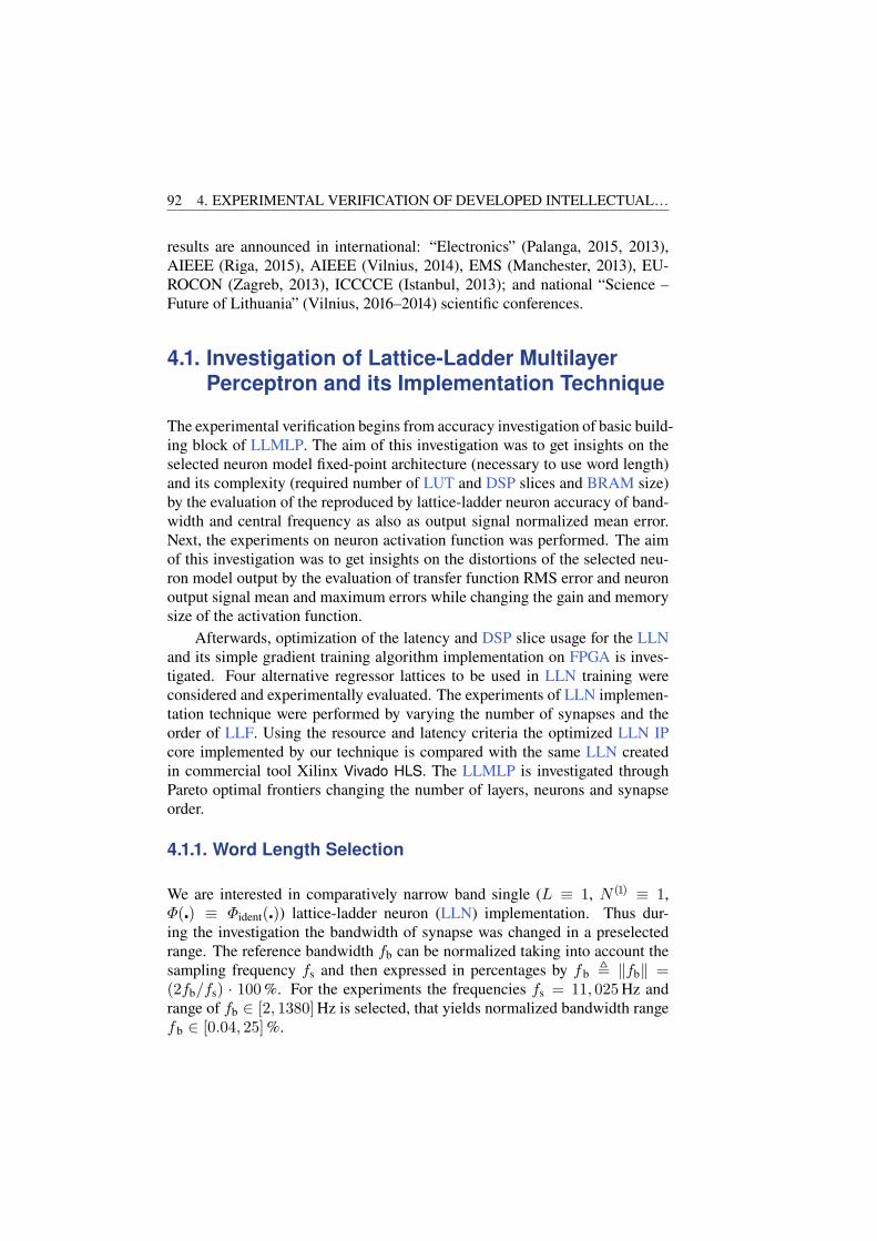
92 4. EXPERIMENTAL VERIFICATION OF DEVELOPED INTELLECTUAL…
results are announced in international: “Electronics” (Palanga, 2015, 2013),AIEEE (Riga, 2015), AIEEE (Vilnius, 2014), EMS (Manchester, 2013), EU-ROCON (Zagreb, 2013), ICCCCE (Istanbul, 2013); and national “Science –Future of Lithuania” (Vilnius, 2016–2014) scientific conferences.
4.1. Investigation of Lattice-Ladder MultilayerPerceptron and its Implementation Technique
The experimental verification begins from accuracy investigation of basic build-ing block of LLMLP. The aim of this investigation was to get insights on theselected neuron model fixed-point architecture (necessary to use word length)and its complexity (required number of LUT and DSP slices and BRAM size)by the evaluation of the reproduced by lattice-ladder neuron accuracy of band-width and central frequency as also as output signal normalized mean error.Next, the experiments on neuron activation function was performed. The aimof this investigation was to get insights on the distortions of the selected neu-ron model output by the evaluation of transfer function RMS error and neuronoutput signal mean and maximum errors while changing the gain and memorysize of the activation function.
Afterwards, optimization of the latency and DSP slice usage for the LLNand its simple gradient training algorithm implementation on FPGA is inves-tigated. Four alternative regressor lattices to be used in LLN training wereconsidered and experimentally evaluated. The experiments of LLN implemen-tation technique were performed by varying the number of synapses and theorder of LLF. Using the resource and latency criteria the optimized LLN IPcore implemented by our technique is compared with the same LLN createdin commercial tool Xilinx Vivado HLS. The LLMLP is investigated throughPareto optimal frontiers changing the number of layers, neurons and synapseorder.
4.1.1. Word Length Selection
We are interested in comparatively narrow band single (L ≡ 1, N (1) ≡ 1,Φ(�) ≡ Φident(�)) lattice-ladder neuron (LLN) implementation. Thus dur-ing the investigation the bandwidth of synapse was changed in a preselectedrange. The reference bandwidth fb can be normalized taking into account thesampling frequency fs and then expressed in percentages by fb , ‖fb‖ =(2fb/fs) · 100%. For the experiments the frequencies fs = 11, 025Hz andrange of fb ∈ [2, 1380]Hz is selected, that yields normalized bandwidth rangefb ∈ [0.04, 25]%.

4. EXPERIMENTAL VERIFICATION OF DEVELOPED INTELLECTUAL… 93
The normalized white noise signal is used as an input sin(n) ≡ ω(n).The neuron training circuit is considered to be correct if all Θj and vj weightsrepresented in fixed-point arithmetics converge to the corresponding truncatedparameters from the reference design. Therefore, the magnitude responses forthe LLN with and without regressor lattice are the same.
The 18 b and 25 b precision is investigated because of FPGA constrains –one and two DSP slices are required to multiply corresponding word lengthsignals. The 10 b and 12 b precision is taken as the possible alternative imple-mentation for low accuracy LLN.
Bandwidth and central frequency relative errors ǫb, ǫc by (2.15) as well asoutput signal normalized MAE EMA by (2.16) were estimated for each specificreference bandwidth fb LL neuron implementation and afterwards correspond-ing normalized relative errors ǫb(fb), ǫc(fb) additionally were calculated. Ac-curacy results for different word length implementations are summarized inFig. 4.1. From Fig. 4.1a follows that the narrow band filter requires denser gridon zero-pole plane near the unit circle. The narrower band is, the more bits arenecessary to preserve low normalized relative error ǫb of the bandwidth.
While enlarging the bandwidth the ǫb decreases exponentially. The LLFwith wider bandwidth reach the same ǫb as LLF with higher precision, i.e., 12 bLLF with band of fb = 7% has same 0.1% mean error as 18 b LLF with bandof fb = 0.1% (Fig. 4.1a). Increase of the LLF precision not evenly improvesthe ǫb for all bandwidths. The reason is in constrained address width of sinΘj
and cos−1Θj implemented in LUTs.
For the narrow band filter until fb = 0.5% the central frequency mean er-rors ǫc don’t depend on implementation precision and exponentially decreasewhile expanding the bandwidth (Fig. 4.1b). The use of one or two DSP slicesgives the same ǫc below fb = 20%. The output signal mean error (seeFig. 4.1c) decreases exponentially for wider normalized reference bandwidth.The replacement of DSP slice by the LUT-based multiplier can be consideredwhen fb ≥ 10%.
4.1.2. Neuron Activation Function Implementation
We are interested in compact and enough precise hyperbolic tangent activa-tion function Φtanh(�) for lattice-ladder neuron implementation. Therefore, thetransfer function and output signal discrepancies are measured under differentBRAM size. During experiments BRAM size is increased 2 times in each stepfrom 64B to 64 kB. The gain is increased linearly from 2 to 16. Other LLNparameters are kept unchanged. Independent on the BRAM size two bytes pre-cision is used for each sample of the approximated hyperbolic tangent. The

94 4. EXPERIMENTAL VERIFICATION OF DEVELOPED INTELLECTUAL…
101
100
101
103
102
101
100
101
102
Normalized bandwidth, f b [%]
−
−
−−
Ban
dwid
thno
rm.
erro
r,ǫ b
[%]
a)
101
100
101
103
102
101
100
101
Normalized bandwidth, f b [%]
−
−
−−
Cen
tral
freq
.no
rm.
erro
r,ǫ c
[%]
b)
101
100
101
102
101
100
101
102
Normalized bandwidth, f b [%]
−
−−O
utpu
tsig
naln
orm
.M
AE
,EM
A[%
]
10 b12 b18 b (1 DSP)25 b (2 DSP)
c)
Fig. 4.1. Accuracy results for the second order lattice-ladder linear neuronand its training circuit implementations on Artix-7 FPGA using different
word length: bandwidth a), central frequency b) and output signal c)normalized errors dependencies on a normalized reference bandwidth
average and maximum errors (EMA and EMM) are obtained by uniformly sam-pling sin(x) on 106 equally spaced points x ∈ [−1, 1].
The average and maximum errors of the activation function output de-pends almost linearly on the LUT size as shown in Table 4.1. In comparisonwith the (Armato et al. 2011), the EMM less than 1.5% can be achieved using512B LUT size or only 0.09% of total BRAM in xc7z020 FPGA chip (Tom-miska 2003) used here for experimental investigation. Maximum error lessthan 0.4% (Xilinx 2013c) can be achieved using 2 kB of BRAM (one of 280available BRAMs in xc7z020) utilizing only 0.36% of total block memory inFPGA chip. The large LUT ensures small error, e.g., 64 kB memory yields

4. EXPERIMENTAL VERIFICATION OF DEVELOPED INTELLECTUAL… 95
EMM = 0.01% and EMM = 0.002% (see Fig. 4.2), however utilizes 11.4% ofavailable memory. Such high precision is very expensive as for single LLN,however is useful for big neural networks with shared activation function.
Table 4.1. The hyperbolic tangent function implementation errors
BRAM size [B] 128 256 512 1k 2k 4k
EMA(RBRAM) [%] 0.54 0.27 0.13 0.06 0.03 0.02EMM(RBRAM) [%] 5.48 2.74 1.39 0.70 0.35 0.16
The maximum EMA is observed at g = 3 for all tested memory sizes(Fig. 4.2). The rising gain allows to access wider range of LUT addresses,therefore decreases the quantization error and EMA falls slowly.
−1
−2
−3
−4
−564
2561k
kk16k
64k 2 4 6 8 10 12 14 16
log10(E
MA)
BRAMsize, R
BRAM [B] Gain, g
Fig. 4.2. The normalized mean absolute error of the lattice-ladder neuronoutput, while changing gain and block random access memory size for
approximated hyperbolic tangent function
The chirp signal with sampling frequency fs = 11, 025Hz and durationN1 = 10 s is used for the transfer function error estimation experiments. Theresults of transfer function RMSE E
ARRMS (g,RBRAM) under two marginal gains
and three different filter bandwidths fb1 = 5512Hz, fb2 = 2756Hz, fb3 =200Hz, are presented in Fig. 4.3, as a dependence on BRAM size. Decrease ofthe bandwidth will reduce the gap between E
ARRMS limits. The E
ARRMS for LLN with
fb1 decreases almost linearly when memory size grows. The lower EAR
RMS =1.2×10⁻⁴ and upper E
ARRMS = 1.8×10⁻³ limits belong to the LLN with widest
bandwidth using 2 kB BRAM for activation function.When LLN is set to pass through all frequencies fb1 = 5512Hz (Fig. 4.4),
then the error EAR
RMS decreases almost linearly increasing both gain and memorysize. The gain set to 2 yields highest error for a given memory size, because at

96 4. EXPERIMENTAL VERIFICATION OF DEVELOPED INTELLECTUAL…
−1
−1.5
−2
−2.5
−3
−3.5
−4
−4.5
−5
−5.5
64 128 256 512 1k 2k 4k 8k 16k 32k 64k
log10E
AR
RM
S
BRAM size, RBRAM [B]
fb1, g=16fb1, g=2
fb2, g=16
fb2, g=2
fb3, g=16
fb3, g=2
1.8×10⁻³
1.2×10⁻⁴
Fig. 4.3. The root mean square error of the lattice-ladder neuron transferfunction using different size look-up tables
g = 2 with the s(x) signal only 1/16 of the approximated hyperbolic tangentcan be accessed. Setting the LLN to work in narrower frequency band fb3
increases the error EAR
RMS for activation function with higher gain and vice versa,smaller gain (less nonlinearity in the activation function) decreases the E
ARRMS.
The increase of BRAM size more than 2 kB nonlinearly improves the error oftransfer function. Therefore, 2 kB BRAM is identified as sufficient memorysize for activation function implementation as a trade-off between resourcesand precision.
The LLN implemented in HLS tool was translated to the low-level modeldescribed in VHDL for further synthesis and uploading to the FPGA. The tim-ing analysis after circuit placement and routing shows that, in the generatedLLN circuit the hyperbolic tangent samples can be accessed with frequencyf⊤ = 312MHz, while f⊤ > 300MHz is considered as a high maximum fre-quency achievable in a practical FPGA systems (Dessouky et al. 2014; Ronak,Fahmy 2014).
4.1.3. Lattice-Ladder Neuron Implementation
The single LLN (Fig. 4.5) is a basic building block of the LLMLP (L ≡ 1,N (1) ≡ 1). In the following novel results on the investigation of a such neuronwith N ≡ N (0) inputs and the M ≡ M (1)th order LLF synapses and togetherwith its training algorithm implementation in FPGA are presented. The mainaim of this investigation is to optimize the latency and DSP slice usage forthe normalized LLN and its gradient training algorithm. Four alternative re-
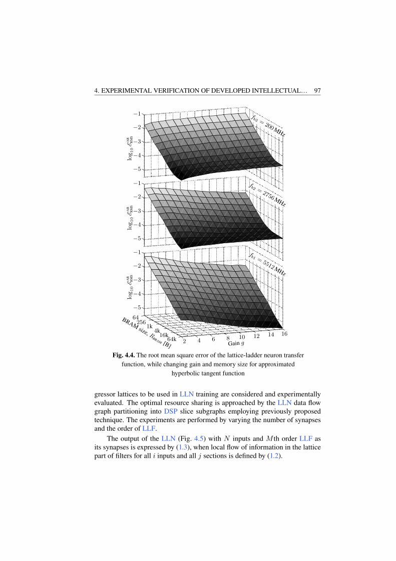
4. EXPERIMENTAL VERIFICATION OF DEVELOPED INTELLECTUAL… 97
−1
−1
−1
−2
−2
−2
−3
−3
−3
−4
−4
−4
−5
−5
−5
64256
1k4k16k
64k 2 4 6 8 10 12 14 16
log10E
AR
RM
Slog10E
AR
RM
Slog10E
AR
RM
S
BRAMsize, R
BRAM [B] Gain g
fb3 =200MHz
fb2 =2756MHz
fb1 =5512MHz
Fig. 4.4. The root mean square error of the lattice-ladder neuron transferfunction, while changing gain and memory size for approximated
hyperbolic tangent function
gressor lattices to be used in LLN training are considered and experimentallyevaluated. The optimal resource sharing is approached by the LLN data flowgraph partitioning into DSP slice subgraphs employing previously proposedtechnique. The experiments are performed by varying the number of synapsesand the order of LLF.
The output of the LLN (Fig. 4.5) with N inputs and M th order LLF asits synapses is expressed by (1.3), when local flow of information in the latticepart of filters for all i inputs and all j sections is defined by (1.2).

98 4. EXPERIMENTAL VERIFICATION OF DEVELOPED INTELLECTUAL…
LLF
LLF
LLFsin1(n)
sin2(n)
sinN (n)
sout(n)Φtanh
Fig. 4.5. The lattice-ladder neuron
A single DSP slice is assigned for each LLN input and additional onefor the δ estimation, thus the use of DSP blocks RDSP
N,M,T depends only on thenumber of synapses, N :
RDSPN,M,T ≡ N + 1. (4.1)
The use of BRAM RBRAMN,M,T depends only on N , too. 8 units of BRAM are
dedicated for non-linear functions and a single unit is used as a buffer for eachof 4 DSP slice inputs, thus:
RBRAMN,M,T ≡ 4(N + 1) + 8. (4.2)
For the comparison purposes, the use of logic resources RLUTN,M,T and achieved
latency RLatN,M,T will be normalized to the maximal value over 4 types of inves-
tigated regressors:
RLUTN,M,T ≡ R
LUTN,M,T
/max
TR
LUTN,M,T; (4.3)
RLatN,M,T ≡ R
LatN,M,T
/max
TR
LatN,M,T , (4.4)
here T – set of considered LLMLP training types, T ∈ {t3, t4, t11, t12}.
The LUT relative utilization RLUTN,M,T and the relative latency R
LatN,M,T are
independent on the number of inputs N , but depend on the LLF order M andregressor type T (see results of experimental study in Fig. 4.6 and Fig. 4.7). IfR
LUTN,M,T = 1 (or RLat
N,M,T = 1), then the implementation of LLN with tx regres-sor is worst in a sense of LUT use (or achieved latency) over all tested typesof regressors at a certain order M of synapses. It is evident that in majorityof cases LLN implementations based on t11 regressor lattice were the worst.Any R
LUTN,M,T or RLat
N,M,T value that is less than one shows how much the im-plementation of LLN with T regressor lattice outperforms the worst case. AtM = 1 the RLUT
N,M,T and RLatN,M,T values are arranged in a same order beginning
from the worst case with t12 regressor to the best case with t3 regressor. TheLLN with t3 regressor saves 16% of FPGA logic resources and has about 10%

4. EXPERIMENTAL VERIFICATION OF DEVELOPED INTELLECTUAL… 99
0 5 10 15 20 25 300.82
0.84
0.86
0.88
0.9
0.92
0.94
0.96
0.98
1
RL
UT
N,M
,T
The order M of lattice-ladder neuron
t3t4t11t12
Fig. 4.6. The relative look-up table usage dependency on the order ofsynapses of lattice-ladder neuron that were implemented in FPGA togetherwith the training scheme based on four different types of regressor lattices
0 5 10 15 20 25 300.88
0.9
0.92
0.94
0.96
0.98
1
RL
atN
,M,T
The order M of lattice-ladder neuron
t3t4t11t12
Fig. 4.7. The relative latency dependency on the order of synapses oflattice-ladder neuron that were implemented in FPGA together with the
training scheme based on four different types of regressor lattices
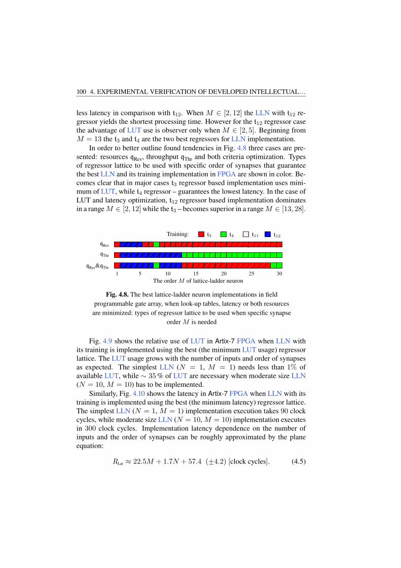
100 4. EXPERIMENTAL VERIFICATION OF DEVELOPED INTELLECTUAL…
less latency in comparison with t12. When M ∈ [2, 12] the LLN with t12 re-gressor yields the shortest processing time. However for the t12 regressor casethe advantage of LUT use is observer only when M ∈ [2, 5]. Beginning fromM = 13 the t3 and t4 are the two best regressors for LLN implementation.
In order to better outline found tendencies in Fig. 4.8 three cases are pre-sented: resources qRes, throughput qThr and both criteria optimization. Typesof regressor lattice to be used with specific order of synapses that guaranteethe best LLN and its training implementation in FPGA are shown in color. Be-comes clear that in major cases t3 regressor based implementation uses mini-mum of LUT, while t4 regressor – guarantees the lowest latency. In the case ofLUT and latency optimization, t12 regressor based implementation dominatesin a range M ∈ [2, 12] while the t3 – becomes superior in a range M ∈ [13, 28].
5 10 15 20 25 301
qRes
qThr
qRes&qThr
The order M of lattice-ladder neuron
Training: t3 t4 t11 t12
Fig. 4.8. The best lattice-ladder neuron implementations in fieldprogrammable gate array, when look-up tables, latency or both resources
are minimized: types of regressor lattice to be used when specific synapseorder M is needed
Fig. 4.9 shows the relative use of LUT in Artix-7 FPGA when LLN withits training is implemented using the best (the minimum LUT usage) regressorlattice. The LUT usage grows with the number of inputs and order of synapsesas expected. The simplest LLN (N = 1, M = 1) needs less than 1% ofavailable LUT, while ∼ 35% of LUT are necessary when moderate size LLN(N = 10, M = 10) has to be implemented.
Similarly, Fig. 4.10 shows the latency in Artix-7 FPGA when LLN with itstraining is implemented using the best (the minimum latency) regressor lattice.The simplest LLN (N = 1, M = 1) implementation execution takes 90 clockcycles, while moderate size LLN (N = 10, M = 10) implementation executesin 300 clock cycles. Implementation latency dependence on the number ofinputs and the order of synapses can be roughly approximated by the planeequation:
RLat ≈ 22.5M + 1.7N + 57.4 (+−4.2) [clock cycles]. (4.5)

4. EXPERIMENTAL VERIFICATION OF DEVELOPED INTELLECTUAL… 101
24
68
10
24
68
100
5
10
15
20
25
30
35
LU
Tut
iliz
atio
n[%
]
The number N of inputs The order M of LLN
Fig. 4.9. The relative use of look-up tables in Artix-7 FPGA whenlattice-ladder neuron with its training is implemented using the best
regressor lattice
24
68
10
2
4
6
8
10
50
100
150
200
250
300
Lat
ency
[clo
ckcy
cles
]
The number N of inputs The order M of LLN
Fig. 4.10. The latency in Artix-7 FPGA when lattice-ladder neuron with itstraining is implemented using the best regressor lattice
The timing analysis of the LLN and its training circuit after placementand routing stage in ISE Design Suite 14.7 shows that the FPGA implementedneuron can be clocked at 300MHz. Therefore, the LLN with 10 inputs and10th order synapses can process input data and learn at a million samples persecond speed.

102 4. EXPERIMENTAL VERIFICATION OF DEVELOPED INTELLECTUAL…
4.1.4. Single Layer of Lattice-Ladder Multilayer PerceptronImplementation
The LLN IP core generated by our technique is compared with the same LLNcore created in Xilinx Vivado HLS tool. For each NPE it is selected the iden-tical 18 b precision for signal width. The neurons in both designs are imple-mented in the way shown in Fig. 2.9 dedicating NPE for each synapse and oneadditional for summation of synapse outputs and instantaneous error calcula-tion. The both generated HDL designs of the IP cores are synthesized, mapped,placed and routed in Xilinx ISE Design Suite 14.7. The resource and timingreports are used to evaluate the performance of the implemented designs underthe maximal sampling frequency fs, LUT equivalent resources and recalculatethe quality criteria: q⋆
Thr and q⋆
Res.The ratio of throughput criteria q
⋆
Thr / qHLSThr shows how much faster the
LLN can sample and learn the signals exploiting our design in comparison withVivado HLS. The ratio of the sampling frequency depends on the synapse orderM and the type of regressor lattice, as shown in Fig. 4.11. It will not dependon number of neurons and layers, since their parallel implementation. The ratioof qThr grows with the increasing of M and is in a range 3–11. The high ratiois affected by the relatively low maximal clock frequency fHLS
s of the VivadoHLS generated cores, e.g., the synapse cores with a training type t3, t4, t11, t12can be clocked by maximal frequencies 174MHz, 179MHz, 179MHz, and158MHz respectively. However, synapse IP core generated by our technique
0 2 4 6 8 10 12 14 16 18 203
4
5
6
7
8
9
10
11
12
t3t4t11t12
q⋆ T
hr/q
HL
ST
hr[t
imes
]
The order M of Lattice-Ladder Neuron
Fig. 4.11. The qThr criteria rate dependency on the order of synapses oflattice-ladder neuron that were implemented in FPGA together with the
training scheme based on four different types of regressor lattices

4. EXPERIMENTAL VERIFICATION OF DEVELOPED INTELLECTUAL… 103
0 2 4 6 8 10 12 14 16 18 200.4
0.5
0.6
0.7
0.8
0.9
1
1.1
t3t4t11t12
q⋆ R
es/q
HL
SR
es[t
imes
]
The order M of Lattice-Ladder Neuron
Fig. 4.12. The ratio of resource criteria qRes dependent on the order ofsynapses of lattice-ladder neuron that were implemented in FPGA togetherwith the training scheme based on four different types of regressor lattices
can be clocked at 320MHz. The Vivado HLS cores also requires more clockcycles to process signals inducing largest latency. The highest clock frequencyand lowest processing latency of our cores yields the qThr criteria improvementup to 11 times.
The ratio of the resource criteria q⋆
Res / qHLSRes shows how many times our
LLN core outperforms the Vivado HLS generated one in terms of LUT equiv-alent resource utilization. In range of M ∈ [2, 4] our core is advantageous,however in other M cases the Vivado HLS design uses less resources and theutilization curve decreases with rising M , as is shown in Fig. 4.12.
The evaluation of the LLN performance through both qThr and qRes multi-plied ratios shows, that our compiler generates at least 3 times more efficientcore in comparison with Vivado HLS. Due to the Vivado HLS tool can notproperly distinguish the DSP supportable subgraphs of LLN, our core com-piler outperforms it by 3–10 times in investigated M ∈ [1, 20] range.
4.1.5. Qualitative Lattice-Ladder Multilayer PerceptronImplementation
The investigation of LLMLP is performed changing the number of neuronsN in each layer, synapse order M and total number of layers L. The LUTand latency optimal type of regressor lattice was selected according to specificsynapse order and qThr, qRes criteria, as it was shown in Fig. 4.8. The results ofdifferent LLMLP configurations are described by Pareto efficient frontiers in

104 4. EXPERIMENTAL VERIFICATION OF DEVELOPED INTELLECTUAL…
Fig. 4.13, Fig. 4.14, Fig. 4.15. Each connected lines of points represent Paretooptimal choices of the possible solutions for certain LLMLP configuration.All other points, which not belongs to Pareto frontier, are not shown here. Thebold dashed lines show resources upper bounds of the existing FPGA fami-lies. These lines helps to select proper FPGA chip for final implementation ofLLMLP core.
0 0.2 0.4 0.6 0.8 1 1.20
0.5
1
1.5
2
2.5
Artix−7
Kintex−7
Virtex−7
L = 2
L = 5
L = 10
L = 20
×106
q−1
Res
qThr [MHz]
Fig. 4.13. Pareto frontiers of lattice-ladder multilayer perceptronimplementation with different number of layers L when M = 10, N = 10
0 1 2 30
0.5
1
1.5
2
2.5
Artix−7
Kintex−7
Virtex−7
M = 2
M = 5
M = 10
M = 20
×106
q−1
Res
qThr [MHz]
Fig. 4.14. Pareto frontiers of lattice-ladder multilayer perceptronimplementation with different orders M when L = 10, N = 10

4. EXPERIMENTAL VERIFICATION OF DEVELOPED INTELLECTUAL… 105
0 0.2 0.4 0.6 0.8 1 1.20
0.5
1
1.5
2
2.5
Artix−7
Kintex−7
Virtex−7
N = 2
N = 5
N = 10
N = 20
×106
q−1
Res
qThr [MHz]
Fig. 4.15. Pareto frontiers of lattice-ladder multilayer perceptronimplementation with different number of neurons N when M = 10, L = 10
All the investigated LLMLP configurations have same tendency reflectedon the Pareto frontiers, where the increase of the throughput criteria qThr givesthe increment of LUT equivalent resources R≡LUT and vice versa. Thereby, itconfirms the state of Pareto efficiency, when it is impossible to make one in-dividual quantity better without making second one worse. The density of thepoints on a front is defined by the optimization process. On the left side ofPareto front it is observed that the optimizer tends to add NPEs to the LLMLPdesign with a small step forming a single layer first. Going to the right side ofthe frontiers the distribution of point is sparse due to larger resource increas-ing step, since the optimizer reproduces the layers and parallelizes forward andbackward pass circuits. The right side points on the frontiers define the maxi-mal sampling frequency for the particular LLMLP. The further increase of themaximal frequency is limited not by the signal latency in the LLMLP circuit,however because of the constrained FPGA resources.
The points in Pareto frontiers, which are above the Virtex-7 bound, showthat there is impossible to implement concrete configuration LLMLP withmaximal sampling frequency on the real 7th series FPGA chips.
4.2. Investigation of Lithuanian SpeechRecognizer
The experimental verification of our created speech recognizer begins with thecomparison to the initial Lithuanian speech recognizer (LSR) devepoled by

106 4. EXPERIMENTAL VERIFICATION OF DEVELOPED INTELLECTUAL…
other researchers (Tamulevičius et al. 2010). Afterwards, the isolated wordrecognition accuracy is comparative evaluated for records of different speak-ers and four features extraction algorithms. The robustness of features extrac-tion algorithms was tested recognizing the speech records at different signalto noise ratios and w/o signal preprocessing using LLN. Finally, the executionspeed of developed IP cores for LSR is experimantally verified.
4.2.1. Comparison with Initial Developments
A previous FPGA implementation (Tamulevičius et al. 2010) was used as abenchmark for the evaluation of the current implementation. Both recognizerswere tested in recognition of the Lithuanian isolated words (loaded to FPGAsequentially as *.wav files) using the same LFCC features extraction.
The used dictionary in both implementations contains 100 unique words.All these words are often used in daily speech: 51 nouns, 23 verbs, 8 adjec-tives, 6 conjunctions, 5 adverbs, 4 pronouns and 3 prepositions. The dictionarycontains: 1 word with 1 syllable, 57 words with 2 syllables, 31 words with3 syllables, 7 words with 4 syllables, and 1 word with 5 syllables.
Recognizers were tested in a speaker dependent mode. All utterances wererecorded in the office environment. 10 speakers (5 females and 5 males) par-ticipated to record the utterances. 10 sessions of 100 words were recorded foreach speaker. Records of first 6 sessions were used in creation of the dictionary.Recognizers were tested using records of remaining 4 sessions. The average97.7% recognition rate over 40 experiments is achieved for the current imple-mentation against 92.8% for the previous implementation (see 1 and 4 columnsin Table 4.2).
The important difference between previous and current recognizers is inthe speech sampling frequency. The current fully hard-core implementationof the Lithuanian isolated word recognition uses a higher sampling frequency(fs = 11.025 kHz), thus gives the 4.9% better recognition accuracy in compar-ison with the FPGA based soft-core implementation (fs = 6 kHz). It is worthmentioning that in the hard-core implementation only integer types of dataare used, while in the soft-core implementation – float type of data was used.Moreover, the signal quantized in 16 b was used in the previous soft-core basedimplementation. In the current implementation an incoming speech signal isquantized in 8 b. Despite the principal algorithm changes and simplifications(particularly in FFT data depth and logarithm computation) it does not reducesthe speaker dependent recognition rate.
Recognizers under investigation use the same dictionary, thus the durationof their recognition sub-processes can be directly compared. Only differencebetween clock frequencies needs to be taken into account. The sub-process
4. EXPERIMENTAL VERIFICATION OF DEVELOPED INTELLECTUAL… 107
Table 4.2. Lithuanian isolated word recognition results
Recognition StageTime Clock Recognition
[ms] [MHz] Rate [%]
Previous Implementation (fs = 6 kHz)
Feature Extraction 1370.000100 92.8
Comparison 22.400Current Implementation (fs = 11.025 kHz)
Feature Extraction 8.52050 97.7Comparison 0.333
Comparison (with constr.) 0.128Improvement [times]
Feature Extraction 1602 +5 %Comparison 67
Comparison (with constr.) 174
of feature extraction (from 1.5 s duration signal) takes 1370ms and 8.52msin previous initial and current implementations correspondingly (see columns1–3 of Table 4.2). The hard-core implemented LFCC features extraction isaccelerated 160 times, despite the used 1.8 times higher signal sampling fre-quency and twice lower main clock frequency. That actually recalculates to320 times (160×2) speed up of feature extraction process.
The right way to evaluate the comparison sub-process is to measure thetime required to calculate one DTW in both implementations. It appears that22.407ms is required in the previous implementation and 0.333ms in thecurrent implementation (without constraints) to calculate one DTW. The ad-ditional use of border constraints reduced the DTW calculation duration to0.128ms, thus 348 times higher acceleration was achieved.
It is important to emphasize that the current recognizer is able to computeapproximately 7800DTW/s at a relatively low (compared with CPU or GPU)50MHz clock frequency. On the other hand, only 1 s is needed to find the bestmatch of up to 1.5 s duration signal features in the dictionary of records withthe total length of 11700 s (3.2 h). In order to take this advantage fully theconnection speed of approximately 17MB/s with the external dictionary hasto be ensured.
A hard-core implementation of the Lithuanian isolated word recognitionutilizes in total 38% of FPGA slice memory, as is shown in Fig. 4.16. It is1.75 times less than the soft-core based algorithm implementation. There isenough logic memory space to duplicate a few DTW units and run them inparallel to reduce the comparison time. The amount of DSP slices is reducedfrom 35 to 21 units. The total number of BRAM units is increased by 46%,

108 4. EXPERIMENTAL VERIFICATION OF DEVELOPED INTELLECTUAL…
0
10
20
30
40
50
60
70
80
90
100
Slices BRAMs DSPs
Unused
Others
DTW
Cepstrum
CI CI CIPI PI PI
Used in PI
%
CI PI
LUTs
FP
GA
res
ourc
e u
sag
e
Fig. 4.16. Comparative FPGA utilization in: previous implementation (PI)and current implementation (CI) versions
because the context dictionary is stored in the internal FPGA memory for fastfeatures access. The number of LUTs is reduced by 7% in comparison withthe previous initial LSR implementation, as shown in Fig. 4.16.
4.2.2. Recognition Accuracy Tune-Up
The dictionary contains the isolated Lithuanian words pronounced by 5 maleand 5 female speakers. 4 sessions of 100 words were recorded for each speakerin the office environment. The first session was used for the training and therest 3 sessions were used for the testing. The recognition rate was tested us-ing original records and using the same words with 30 dB and 15 dB signal tonoise ratios (SNR). The aim is to determine most suitable features extractionalgorithm among MFCC, LFCC, LPCC and LPC for speaker dependent reco-gnizer. The averaged results over male and female speakers without filteringIP core are given in Table 4.3. The best average recognition rate was achievedfor original records using MFCC (93.2%) and LFCC (93.0%) features. TheLFCC (90.8%) and little less LPCC (89.8%) features are more robust to noisewhen SNR is 30 dB. The LPCC (83.7%) features give better recognition accu-racy when SNR is 15 dB. The LPC features give the worst recognition rates inall cases, comparing with others features extraction algorithms.
The recognition accuracy highly depends on speaker gender, tone of voice,articulation and speed of pronunciation. It is important to diagnose the rea-sons of differences in rates while using same features extraction method. Eachentry in the Table 4.4 and Table 4.5 evaluates the recognition accuracy overthree times repeated experiments. In the male (Mi) speaker case there are twospeakers (M1 and M2) with high recognition accuracy over all features ex-

4. EXPERIMENTAL VERIFICATION OF DEVELOPED INTELLECTUAL… 109
Table 4.3. Averaged isolated word recognition results
FeaturesOriginal Records with Records with
records SNR = 30 dB SNR = 15 dB
MFCC 93.2 86.7 79.3
LFCC 93.0 90.8 72.4
LPCC 91.5 89.8 83.7
LPC 82.5 78.6 67.1
Table 4.4. Isolated word recognition rates for male speakers [%]
Speaker M1 M2 M3 M4 M5 Average With LLN
MFCC
Original 100 98 91 83 86 91.6 030 dB 90 95 83 76 78 84.4 +2.215 dB 87 92 77 62 66 76.8 +5.0LFCC
Original 99 97 91 84 89 92.0 030 dB 96 94 79 83 91 88.6 +1.815 dB 91 72 65 69 75 74.4 +5.1LPCC
Original 99 95 90 77 79 88.0 030 dB 94 91 77 84 88 86.8 +0.815 dB 93 85 72 79 77 81.2 +4.5LPC
Original 91 85 73 68 57 74.8 030 dB 79 82 57 66 64 69.6 +1.615 dB 82 64 48 57 56 61.4 +2.8
traction methods and different SNRs. There are speakers (M4 and M5) withrelatively lower rates comparing with others. These two speakers have lowtone of voice, therefore the spectral information is distributed in low frequencydomain. Some errors are caused by different pronunciation of the same wordin the following sessions.
In the case of female speakers (Fi) the F2 has lowest rate. In the F2 recordsthe low-frequency periodic noise is observed. The speaker F5 pronounces thewords faster than F1, F3 and F4. It influences the accuracy, as is shown inTable 4.5. The average recognition rate of the female records outperforms therate of male records in all features extraction cases (Fig. 4.17). The confidenceinterval of recognition accuracy with 0.95 probability was calculated from theBeta distribution law approximated by χ2 distribution (Kruopis 1993). Otherresearchers declare similar 91–96% recognition rates in the speech recognitionsystems based on software (Lileikytė, Telksnys 2011; Maskeliūnas, Esposito

110 4. EXPERIMENTAL VERIFICATION OF DEVELOPED INTELLECTUAL…
Table 4.5. Isolated word recognition rates for female speakers [%]
Speaker F1 F2 F3 F4 F5 Average With LLN
MFCC
Original 98 87 98 99 92 94.8 030 dB 94 82 91 97 81 89.0 +1.815 dB 92 76 83 93 65 81.8 +4.7LFCC
Original 95 86 95 99 95 94.0 030 dB 95 85 93 98 94 93.0 +0.215 dB 67 65 72 81 67 70.4 +4.2LPCC
Original 97 89 98 99 92 95.0 030 dB 97 85 93 99 90 92.8 +0.615 dB 87 74 83 98 89 86.2 +4.9LPC
Original 93 87 92 97 82 90.2 030 dB 89 81 92 95 81 87.6 +0.815 dB 72 66 73 87 66 72.8 +3.3
...
...
...
......
...
92
95
89
93
81
86
0 60 70 80 90 100 [%]
SN
R15
dBS
NR
30
dBO
rigi
nal
Recognition rate
Mi
Mi
Mi
Fi
Fi
Fi
MFCCLFCCLPCCLPC
Fig. 4.17. The average recognition rate of isolated word pronounced by maleand female speaker using different features extraction algorithms
2012; Wijoyo 2011; Zhou et al. 2011) and hardware (Cheng et al. 2011; Pan, Li2012; Zhang et al. 2011) implementations.
The last column in Table 4.4 and Table 4.5 shows the recognition rateimprovement using the LLN (Fig. 4.5) in filtering IP core. The experiments
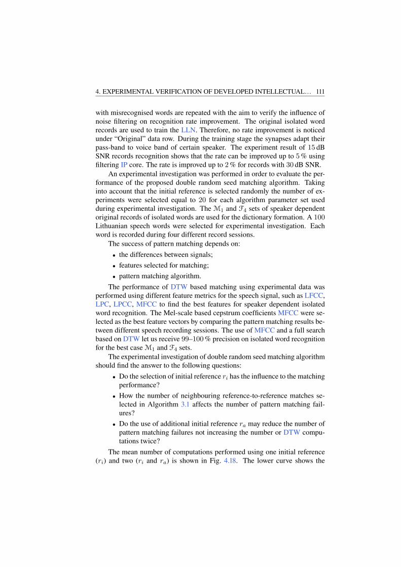
4. EXPERIMENTAL VERIFICATION OF DEVELOPED INTELLECTUAL… 111
with misrecognised words are repeated with the aim to verify the influence ofnoise filtering on recognition rate improvement. The original isolated wordrecords are used to train the LLN. Therefore, no rate improvement is noticedunder “Original” data row. During the training stage the synapses adapt theirpass-band to voice band of certain speaker. The experiment result of 15 dBSNR records recognition shows that the rate can be improved up to 5% usingfiltering IP core. The rate is improved up to 2% for records with 30 dB SNR.
An experimental investigation was performed in order to evaluate the per-formance of the proposed double random seed matching algorithm. Takinginto account that the initial reference is selected randomly the number of ex-periments were selected equal to 20 for each algorithm parameter set usedduring experimental investigation. The M1 and F4 sets of speaker dependentoriginal records of isolated words are used for the dictionary formation. A 100Lithuanian speech words were selected for experimental investigation. Eachword is recorded during four different record sessions.
The success of pattern matching depends on:
• the differences between signals;
• features selected for matching;
• pattern matching algorithm.
The performance of DTW based matching using experimental data wasperformed using different feature metrics for the speech signal, such as LFCC,LPC, LPCC, MFCC to find the best features for speaker dependent isolatedword recognition. The Mel-scale based cepstrum coefficients MFCC were se-lected as the best feature vectors by comparing the pattern matching results be-tween different speech recording sessions. The use of MFCC and a full searchbased on DTW let us receive 99–100% precision on isolated word recognitionfor the best case M1 and F4 sets.
The experimental investigation of double random seed matching algorithmshould find the answer to the following questions:
• Do the selection of initial reference ri has the influence to the matchingperformance?
• How the number of neighbouring reference-to-reference matches se-lected in Algorithm 3.1 affects the number of pattern matching fail-ures?
• Do the use of additional initial reference ra may reduce the number ofpattern matching failures not increasing the number or DTW compu-tations twice?
The mean number of computations performed using one initial reference(ri) and two (ri and ra) is shown in Fig. 4.18. The lower curve shows the

112 4. EXPERIMENTAL VERIFICATION OF DEVELOPED INTELLECTUAL…
0 2 4 6 8 10 120
500
1000
1500
2000
2500
3000
3500
4000
4500
Double search
Single search
Number of neighbouring references
Num
ber
ofD
TW
com
puta
tion
s
Fig. 4.18. Illustration of the computational load dependence on the numberof selected neighbouring references
0 2 4 6 8 10 120
10
20
30
40
50
60
70
80
90
100
Double search
Single search
Number of neighbouring references
Rec
ogni
tion
accu
racy
[%]
Fig. 4.19. Pattern match rate dependence on the number of selectedneighbouring references
amount of DTW computations performed to make a decision accordingly tothe rule of the Algorithm 3.1, proposed in Section 3.3. The upper curve showsthe total number of DTW computations that should be performed if additionalreference ra is used for matching. It can be noticed, that the total amount ofcomputations rises with lower speed comparing to the situation with only onereference (ri) selected. However we should notice also, that at least 30% ofreferences should be compared to make a decision when both ri and ra areused.

4. EXPERIMENTAL VERIFICATION OF DEVELOPED INTELLECTUAL… 113
The use of additional reference ra increases the precision of pattern match-ing significantly (Fig. 4.19). Comparing the number of correctly matched ref-erences (Fig. 4.19) and the number of computations performed (Fig. 4.18) wesee that the double increase of the number of neighbouring references, usedfor matching, has a little impact to the number of correctly matched patterns.Additional 3–4% of matching precision may cost the increase of number ofDTW computations from 30% to 38%.
The matching rate should be always put in front of the computational loadof the algorithm. However for the real-time application of the algorithm, e.g.,implementation of the algorithm in speech recognition based portable con-troller, the high computational load may limit the size of the dictionary, thatcould be applied and may consume too much power from the battery, makingthe controller not portable anymore.
4.2.3. Execution Speed Determination
The time-line diagram of feature extraction and comparison stages is shownin Fig. 4.20. The gray and white rows mark the amount of time needed forFPGA-based and CPU-based computations respectively (Matlab was used assoftware running on personal computer (PC) with 50% usage of 3GHz CPU).CPU-based MFCC, LPCC and LPC extraction is more than 10 and 5 timesfaster respectively. The higher calculation speed is strongly influenced by 30times higher CPU clock frequency. The advantage of FPGA against CPU isobserved in LFCC and DTW calculations. FPGA-based LFCC runs 1.5 timesfaster than CPU-based because of simplifications in logarithm and FFT coreemployment. FPGA-based DTW and DTWc calculation is speed-up more than280 times in comparison with same algorithm implemented in Matlab.
FPGACPU
MFCC
LPCC
LPC
LFCC
one DTW
one DTWc
3304µs285µs
3349µs313µs
1667µs307µs
66µs102µs
333µs 94100µs
128µs 36320µs
11610µs
The bound forreal-time
processing
0 1000 5000 10000 t [µs]
Fig. 4.20. The time-line diagram of feature extraction and comparisonstages based on FPGA and CPU
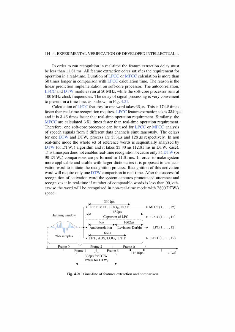
114 4. EXPERIMENTAL VERIFICATION OF DEVELOPED INTELLECTUAL…
In order to run recognition in real-time the feature extraction delay mustbe less than 11.61ms. All feature extraction cores satisfies the requirement foroperation in a real-time. Duration of LPCC or MFCC calculation is more than50 times longer in comparison with LFCC calculation time. The reason is thelinear prediction implementation on soft-core processor. The autocorrelation,LFCC and DTW modules run at 50MHz, while the soft-core processor runs at100MHz clock frequencies. The delay of signal processing is very convenientto present in a time-line, as is shown in Fig. 4.21.
Calculation of LFCC features for one word takes 66µs. This is 174.8 timesfaster than real-time recognition requires. LPCC feature extraction takes 3349µsand it is 3.46 times faster that real-time operation requirement. Similarly, theMFCC are calculated 3.51 times faster than real-time operation requirement.Therefore, one soft-core processor can be used for LPCC or MFCC analysisof speech signals from 3 different data channels simultaneously. The delaysfor one DTW and DTWc process are 333µs and 128µs respectively. In nonreal-time mode the whole set of reference words is sequentially analyzed byDTW (or DTWc) algorithm and it takes 33.30ms (12.81 ms in DTWc case).This timespan does not enables real-time recognition because only 34 DTW (or90 DTWc) comparisons are performed in 11.61ms. In order to make systemmore applicable and usable with larger dictionaries it is proposed to use acti-vation word to initiate the recognition process. Recognition of this activationword will require only one DTW comparison in real-time. After the successfulrecognition of activation word the system captures pronounced utterance andrecognizes it in real-time if number of comparable words is less than 90, oth-erwise the word will be recognized in non-real-time mode with 7800DTW/sspeed.
. . .
Hanning window
256 samples
Frame 0Frame 1
Frame 2Frame 3
Frame 0
11610µs333µs for DTW
t [µs]
128µs for DTWc
3304µs
1682µs
Cepstrum of LPC
5µs 1662µs
66µs
FFT, ABS, LOG2, FFT
FFT, MEL, LOG2, DCT
Autocorrelation Levinson-Durbin
MFCC(1, . . . , 12)
LPCC(1, . . . , 12)
LPC(1, . . . , 12)
LFCC(1, . . . , 12)
Fig. 4.21. Time-line of features extraction and comparison

4. EXPERIMENTAL VERIFICATION OF DEVELOPED INTELLECTUAL… 115
The fastest version of software-based comparison process (Tamulevičiuset al. 2010) is speeded-up 134 times using DTW algorithm and 348 times us-ing DTWc algorithm. LFCC feature extraction is speeded-up 160 times. Theaverage recognition rate is improved by 1 % (up to 94%) using LFCC and by2% (up to 95%) using LPCC and MFCC features. Other researchers declaresimilar recognition rates of 90–93% on hardware-based speech recognizers(Cheng et al. 2011; Choi et al. 2010; Pan et al. 2011; Veitch et al. 2010; Zhanget al. 2011).
4.3. Conclusions of the 4th Chapter
1. The application of MFCC and LFCC is more suitable for recognitionof clean records. The LFCC and LPCC features are appropriate for30 dB environment noise. The LPCC features gives the best accuracyat 15 dB SNR comparing to other algorithms at same noise level.
2. Using filtering intellectual property (IP) core the recognition rate of15 dB and 30 dB SNR records can be improved up to 5% and 2%respectively.
3. The double random seed matching algorithm reduces the computa-tional load of the classical dynamic time warping (DTW) based speechrecognition algorithm by 62–70% keeping the 90–97% rate of cor-rectly recognised words.
4. Comparing with a previous soft-core recognizer the current hardwarebased implementation accelerates features extraction up to 320 times.The DTW with border constraints is speeded up 348 times.
5. For the investigated neuron with the bandwidth wider than 10% ofnormalized reference bandwidth even 10 b word length representationis appropriate as its output signal mean error is less than 1%.
6. The use of t11 regressor lattice must be avoided. For look-up table(LUT) critical lattice-ladder neuron (LLN) implementations regressorlattice t3 has to be used when M ≥ 6. For latency critical LLN im-plementations two regressor lattices are superior: t12 (M ∈ [2, 12]), t3(M ≤ 13). For LUT and latency critical LLN implementations (witha few exceptions M = {1, 8}) the same regressor lattices are superior:t12 (M ∈ [2, 12]) and t3 (M ∈ [13, 28]).
7. Block RAM size of 2 kB is sufficient to achieve tolerable less than0.4% maximum error of the approximated activation function outputwith small RMS error E
ARRMS = 1.8×10⁻³ of the lattice-ladder neuron
transfer function.

116 4. EXPERIMENTAL VERIFICATION OF DEVELOPED INTELLECTUAL…
8. The corresponding lattice-ladder multilayer perceptron (LLMLP) com-piler generates at least 3 times more efficient LLMLP core in compar-ison with Vivado HLS tool.
9. The Pareto efficient frontiers allows to properly select concrete FPGAchip according to required amount of resources, maximal data sam-pling frequency and LLMLP structure.

General Conclusions
The problem of efficient and straightforward implementation of operating ina real-time electronic intelligent systems on FPGA was solved. The followingsignificant results for scientific field of Electrical and Electronic engineeringare obtained:
1. The technique for lattice-ladder multilayer perceptron (LLMLP) effi-cient implementation in FPGA is created and experimentally affirmed:
1.1. The corresponding LLMLP compiler generates at least 3 timesmore efficient core in comparison with Vivado HLS tool.
1.2. The developed neuron processing element based on FPGA DSPslice structure guarantees less than 1% output signal mean abso-lute error, ǫT = 1.8×10⁻³ root mean square error of the lattice-ladder neuron transfer function and is speed optimal with only7 clock cycle latency.
1.3. The elucidated experimental evidence grounded knowledge on thequickest training algorithms of LLMLP and the best lattice regres-sors T ∈ {t3, t4, t11, t12} use for look-up table (LUT) and latencycritical implementations is incorporated in the technique.
2. Pareto frontiers estimation for the LLMLP specialized criteria of cir-cuitry synthesis is proposed:
2.1. An optimal choice of FPGA chip according to given requirementsfor LLMLP structure, sampling frequency and other resources isdone.
117

118 GENERAL CONCLUSIONS
2.2. Two implementation strategies: throughput or resource optimiza-tion, are developed.
3. The optimized FPGA intellectual property (IP) cores are developedand experimentally verified in Lithuanian speech recognizer:
3.1. The use of the lattice-ladder neuron LLN IP core improves therecognition rate at least by 4% for 15 dB SNR records.
3.2. The application of MFCC and LFCC IP cores is suitable for recog-nition of clean records. Moreover the LFCC and LPCC IP coresare appropriate for use at 30 dB SNR, while only the LPCC deliv-ers the best accuracy at 15 dB SNR.
3.3. Hardware optimized single isolated word matching (DTWc) IP coreexecutes in 128µs achieving 7800word/s comparison speed.
4. A first working prototype of Lithuanian speech recognizer in FPGA fordisabled persons is created and tested:
4.1. A new accelerated pattern matching algorithm uses constraineddynamic time warping and enables to recognize words 2.6 timesquicker without the loose of recognition accuracy at 97%.
4.2. The use of a new double random seed matching algorithm addi-tionally can speed up the recognition up to 2.6 times with a disad-vantage of recognition accuracy reduction till 90%.

References
Ai, O. C.; Hariharan, M.; Yaacob, S.; Chee, L. S. 2012. Classification of Speech Dys-fluencies with MFCC and LPCC Features, Expert Systems with Applications 39(2):2157–2165. [see 37 p.]
Alberto de Albuquerque Silva, C.; Duarte Doria Neto, A.; Alberto Nicolau Oliveira,J.; Dantas Melo, J.; Simonetti Barbalho, D.; Medeiros Avelino, A. 2015. Definition ofan architecture to configure artificial neural networks topologies using partial recon-figuraton in FPGA, Latin America Transactions, IEEE (Revista IEEE America Latina)
13(7): 2094–2100. [see 29 p.]
Alecsa, B.; Cirstea, M.; Onea, A. 2012. Simulink modeling and design of an effi-cient hardware-constrained FPGA-based PMSM speed controller, IEEE Transactions
on Industrial Informatics 8: 554–562. ISSN 1551-3203. [see 10 p.]
Altera 2013. Chip Editor [interactive] [14 March 2014]. Prieiga per inter-netą: <http://www.altera.com/literature/hb/qts/qts_qii52006.pdf>.[see 32 p.]
Altera 2014. FFT IP Core User Guide [interactive] [25 August 2015].Prieiga per internetą: <https://www.altera.com/content/dam/altera-www/global/en_US/pdfs/literature/ug/ug_fft.pdf>. [see 38 p.]
Amin, H.; Curtis, K.; Hayes-Gill, B. 1997. Piecewise linear approximation applied tononlinear function of a neural network, Circuits, Devices and Systems, IEE Proceed-
ings - 144(6): 313–317. ISSN 1350-2409. [see 33 p.]
Amin, H.; Curtis, K.; Hayes Gill, B. 1999. Two-ring systolic array network for artificial
119

120 REFERENCES
neural networks, Circuits, Devices and Systems, IEE Proceedings - 146(5): 225–230.ISSN 1350-2409. [see 31 p.]
Amudha, V.; Venkataramani, B.; Manikandan, J. 2008. FPGA implementation ofisolated digit recognition system using modified back propagation algorithm, in Proc.
ICED’08, 1–6. [see 36, 41 p.]
Anguita, D.; Carlino, L.; Ghio, A.; Ridella, S. 2011. A FPGA core generator forembedded classification systems, Journal of Circuits, Systems, and Computers 20(2):263–282. ISSN 0218-1266. [see 28 p.]
Anguita, D.; Ghio, A.; Pischiutta, S.; Ridella, S. 2008. A support vector machine withinteger parameters, Neurocomputing 72(1?3): 480 – 489. ISSN 0925-2312. [see 28 p.]
Arias-Garcia, J.; Braga, A.; Llanos, C. H.; Ayala-Rincon, M.; Pezzuol Jacobi, R.;Foltran, A. 2013. FPGA HIL simulation of a linear system block for strongly cou-pled system applications, in Industrial Technology (ICIT), 2013 IEEE International
Conference on, 1017–1022. ISBN 978-1-4673-4567-5. [see 10 p.]
Armato, A.; Fanucci, L.; Scilingo, E. P.; De Rossi, D. 2011. Low-error digital hard-ware implementation of artificial neuron activation functions and their derivative, Mi-
croprocessors and Microsystems 35(6): 557–567. [see 29, 30, 67, 94 p.]
Arminas, V.; Tamulevicius, G.; Navakauskas, D.; Ivanovas, E. 2010. Acceleration offeature extraction for FPGA-based speech recognition, in Photonics Applications in
Astronomy, Communications, Industry, and High-Energy Physics Experiments 2010,International Society for Optics and Photonics, 511–516. [see 35 p.]
Atri, M.; Sayadi, F.; Elhamzi, W.; Tourki, R. 2012. Efficient Hardware/SoftwareImplementation of LPC Algorithm in Speech Coding Applications, Journal of Signal
and Information Processing 3(9): 122–129. [see 37, 40 p.]
Back, A. D.; Tsoi, A. C. 1993. A simplified gradient algorithm for iir synapse multi-layer perceptrons, Neural Computation 5(3): 456–462. [see 16 p.]
Bahoura, M. 2014. FPGA implementation of high-speed neural network for power am-plifier behavioral modeling, Analog Integrated Circuits and Signal Processing 79(3):507–527. [see 29, 30 p.]
Bahoura, M.; Ezzaidi, H. 2013. Hardware implementation of mfcc feature extractionfor respiratory sounds analysis, in 8th Workshop on Systems, Signal Processing and
their Applications, 226–229. [see 38, 39 p.]
Beiu, V. 1998. How to build vlsi-efficient neural chips, in Proceedings of the Interna-
tional ICSC Symposium on Engineering of Intelligent Systems, 66–75. [see 33 p.]
Bosque, G.; del Campo, I.; Echanobe, J. 2014. Fuzzy systems, neural networks andneuro-fuzzy systems: A vision on their hardware implementation and platforms overtwo decades, Engineering Applications of Artificial Intelligence 32(1): 283–331. ISSN0952-1976. [see 16 p.]
Broersen, P. M. 1994. A comparison of transfer function estimators, in Instrumentation

REFERENCES 121
and Measurement Technology Conference, 1994. IMTC/94. Conference Proceedings.
10th Anniversary. Advanced Technologies in I & M., 1994 IEEE, IEEE, 1377–1380. [see 68 p.]
Buyukkurt, B.; Najjar, W. A. 2008. Compiler generated systolic arrays for wavefrontalgorithm acceleration on FPGAs, in Proc. FPL’08, 655–658. [see 42 p.]
Cadence 2013. C-to-Silicon Compiler High-Level Synthesis [interactive] [10 Decem-ber 2013]. Prieiga per internetą: <http://www.cadence.com/rl/Resources/datasheets/C2Silicon_ds.pdf>. [see 14 p.]
del Campo, I.; Finker, R.; Echanobe, J.; Basterretxea, K. 2013. Controlled accuracyapproximation of sigmoid function for efficient FPGA-based implementation of arti-ficial neurons, Electronics Letters 49(25): 1598–1600. [see 29, 30 p.]
Carrillo, S.; Harkin, J.; Mcdaid, L.; Pande, S.; Cawley, S.; Mcginley, B.; Morgan, F.2012. Advancing interconnect density for spiking neural network hardware implemen-tations using traffic-aware adaptive network-on-chip routers, Neural Netw. 33: 42–57.ISSN 0893-6080. [see 20 p.]
A look at trends from Consumer Electronics Show [interactive]. 2016. Green TechMedia [14 January 2016]. Prieiga per internetą: <http://www.greentechmedia.com/>. [see 3 p.]
Chakravarty, A. 2014. Speech recognition toolkit for the Arduino [interactive][20 April 2014]. Prieiga per internetą: <http://http://arjo129.github.io/uSpeech/>. [see 35 p.]
Chan, K. Y.; Nordholm, S.; Yiu, K. F. C.; Togneri, R. 2013. Speech enhancementstrategy for speech recognition microcontroller under noisy environments, Neurocom-
puting 118(1): 279–288. ISSN 0925-2312. [see 15 p.]
Chen, D.; Cong, J.; Pan, P. 2006. FPGA design automation: A survey, Foundations
and Trends in Electronic Design Automation 1(3): 195–330. [see 10 p.]
Cheng, O.; Abdulla, W.; Salcic, Z. 2011. Hardware–software codesign of automaticspeech recognition system for embedded real-time applications, Industrial Electron-
ics, IEEE Transactions on 58(3): 850–859. [see 39, 110, 115 p.]
Choi, J.; You, K.; Sun, W. 2010. An FPGA implementation of speech recognitionwith weighted finite state transducers, in Acoustics Speech and Signal Processing
(ICASSP), 2010 IEEE International Conference on, IEEE, 1602–1605. [see 34, 35,115 p.]
Chung, J.-G.; Parhi, K. 1996. Pipelined Lattice and Wave Digital Recursive Filters:The International Series in Engineering and Computer Science. Springer. [see 18 p.]
Chung, J.-G.; Parhi, K. 2012. Pipelined lattice and wave digital recursive filters.Springer Science & Business Media. [see 22 p.]
Chung, J.-H.; Yoon, H.; Maeng, S. R. 1992. A systolic array exploiting the inher-ent parallelisms of artificial neural networks, Microprocess. Microprogram. 33(3):

122 REFERENCES
145–159. ISSN 0165-6074. Prieiga per internetą: <http://dx.doi.org/10.1016/0165-6074(92)90017-2>. [see 31 p.]
Clayton, C. 2008. Digital duct tape with FPGA editor, XCell 66: 54–57. [see 32 p.]
Cong, J.; Jiang, W. 2008. Pattern-based behavior synthesis for FPGA resource re-duction, in Proceedings of the 16th international ACM/SIGDA symposium on Field
programmable gate arrays, 107–116. [see 15, 54 p.]
Cong, J.; Liu, B.; Neuendorffer, S.; Noguera, J.; Vissers, K.; Zhang, Z. 2011. High-level synthesis for fpgas: From prototyping to deployment, Computer-Aided Design of
Integrated Circuits and Systems, IEEE Transactions on 30(4): 473–491. ISSN 0278-0070. [see 15 p.]
Cornu, T.; Ienne, P. 1994. Performance of digital neuro-computers, in Microelectron-
ics for Neural Networks and Fuzzy Systems, 1994., Proceedings of the Fourth Interna-
tional Conference on, 87–93. [see 33 p.]
Czajkowski, T. S. 2008. Physical synthesis toolkit for area and power optimization on
FPGAs: Dissertation. University of Toronto. University of Toronto. 134 p. ISBN978-0-494-57976-3. [see 10 p.]
Darabkh, K. A.; Khalifeh, A. F.; Bathech, B. A.; Sabah, S. W. 2012. Efficient DTW-Based Speech Recognition System for Isolated Words of Arabic Language, World
Academy of Science, Engineering and Technology 77: 85–88. [see 37 p.]
Dessouky, G.; Klaiber, M. J.; Bailey, D. G.; Simon, S. 2014. Adaptive dynamic on-chip memory management for FPGA-based reconfigurable architectures, in Field Pro-
grammable Logic and Applications (FPL), 2014 24th International Conference on,IEEE, 1–8. [see 96 p.]
Ding, H.; Trajcevski, G.; Scheuermann, P.; Wang, X.; Keogh, E. 2008. Querying andmining of time series data: Experimental comparison of representations and distancemeasures, in Proc. VLDB’08, 1542–1552. [see 41 p.]
Dinu, A.; Cirstea, M.; Cirstea, S. 2010. Direct neural-network hardware-implementation algorithm, Industrial Electronics, IEEE Transactions on 57(5): 1845–1848. ISSN 0278-0046. [see 28 p.]
Er, M. J.; Li, Z.; Cai, H.; Chen, Q. 2005. Adaptive noise cancellation using enhanceddynamic fuzzy neural networks, Fuzzy Systems, IEEE Transactions on 13(3): 331–342.[see 16 p.]
Farjo, J.; Aoun, M.; Kassem, A.; Hamouche, M.; et al. 2012. Speaker identification oncompactrio, in Electrotechnical Conference (MELECON), 2012 16th IEEE Mediter-
ranean, IEEE, 399–403. [see 39 p.]
Ferreira, P.; Ribeiro, P.; Antunes, A.; Dias, F. M. 2007. A high bit resolution FPGAimplementation of a fnn with a new algorithm for the activation function, Neurocom-
puting 71(1): 71–77. [see 19, 29, 30 p.]
Finker, R.; del Campo, I.; Echanobe, J.; Doctor, F. 2013. Multilevel adaptive neural

REFERENCES 123
network architecture for implementing single-chip intelligent agents on FPGAs, inNeural Networks (IJCNN), The 2013 International Joint Conference on, 1–9. ISSN2161-4393. [see 18 p.]
Firdauzi, A.; Wirianto, K.; Arijal, M.; Adiono, T. 2013. Design and implementationof real time noise cancellation system based on spectral subtraction method, Procedia
Technology 11(1): 1003–1010. ISSN 2212-0173. [see 16 p.]
Fook, C. Y.; Hariharan, M.; Yaacob, S.; Ah, A. 2012. Malay speech recognition in nor-mal and noise condition, in IEEE 8th International Colloquium on Signal Processing
and its Applications (CSPA 2012), 409–412. [see 37 p.]
Gavat, I.; Militaru, D. M.; Dumitru, C. O. 2008. Knowledge resources in automaticspeech recognition and understanding for Romanian language, InTech Speech Recog-
nition Technologies and Applications 1: 241–260. [see 41 p.]
Gomperts, A.; Ukil, A.; Zurfluh, F. 2011. Development and implementation of param-eterized FPGA-based general purpose neural networks for online applications, Indus-
trial Informatics, IEEE Transactions on 7(1): 78–89. [see 29, 30 p.]
Gray, A. H.; Markel, J. D. 1975. A Normalized Digital Filter Structure, IEEE Trans-
action on Acoustics, Speech, and Signal Processing 23(3): 268–277. [see 22 p.]
Hadei, S. A.; Lotfizad, M. 2011. A family of adaptive filter algorithms in noise can-cellation for speech enhancement, International Journal of Computer and Electrical
Engineering 2(2). [see 16 p.]
Hammerstrom, D. 1990. A vlsi architecture for high-performance, low-cost, on-chiplearning, in Neural Networks, 1990., 1990 IJCNN International Joint Conference on,vol. 2, 537–544. [see 31, 33 p.]
Harkin, J.; Morgan, F.; McDaid, L.; Hall, S.; McGinley, B.; Cawley, S. 2009. Areconfigurable and biologically inspired paradigm for computation using network-on-chip and spiking neural networks, Int. J. Reconfig. Comput. 2009: 1–13. ISSN 1687-7195. [see 20 p.]
Himavathi, S.; Anitha, D.; Muthuramalingam, A. 2007. Feedforward neural networkimplementation in FPGA using layer multiplexing for effective resource utilization,Neural Networks, IEEE Transactions on 18(3): 880–888. [see 29 p.]
Hirsimaki, T.; Kurimo, M. 2004. Decoder issues in unlimited Finnish speech recogni-tion, in Proc. NORSIG’04, 320–323. [see 34, 41 p.]
Holt, J.; Hwang, J.-N. 1993. Finite precision error analysis of neural network hardwareimplementations, Computers, IEEE Transactions on 42(3): 281–290. ISSN 0018-9340. [see 17, 33 p.]
Hussain, S. M. A.; Rashid, A. B. M. 2012. Optimization of VLSI architectures forDTW, in Proc. ICECE’12, 737–740. [see 41 p.]
Ivanovas, E. 2012. Development and implementation of means for word duration sig-
nal processing: Doctoral Dissertation. Vilnius Gediminas Technical University. Vil-

124 REFERENCES
nius: Technika. [see 35 p.]
Johnston, S.; Prasad, G.; Maguire, L.; McGinnity, M. 2005. Comparative investigationinto classical and spiking neuron implementations on FPGAs, in Proceedings of the
15th International Conference on Artificial Neural Networks: Biological Inspirations
- Volume Part I: ICANN’05, 269–274. [see 20 p.]
Kazanavičius, E.; Venteris, R. 2000. Architectures for ultrasonic delay time estimationtasks, Ultragarsas" Ultrasound" 34(1): 23–27. [see 15 p.]
van Keulen, E.; Colak, S.; Withagen, H.; Hegt, H. 1994. Neural network hardware per-formance criteria, in Neural Networks, 1994. IEEE World Congress on Computational
Intelligence., 1994 IEEE International Conference on, vol. 3, 1955–1958. [see 33 p.]
Kim, C.-M.; Park, H.-M.; Kim, T.; Choi, Y.-K.; Lee, S.-Y. 2003. FPGA implementa-tion of ica algorithm for blind signal separation and adaptive noise canceling, Neural
Networks, IEEE Transactions on 14(5): 1038–1046. [see 16 p.]
Kim, D.; Kim, H.; Kim, H.; Han, G.; Chung, D. 2005. A simd neural networkprocessor for image processing, in Proceedings of the Second International Confer-
ence on Advances in Neural Networks - Volume Part II: ISNN’05, Berlin, Heidelberg:Springer-Verlag, 665–672. ISBN 3-540-25913-9. [see 31 p.]
Kruopis, J. 1993. Matematinė statistika: vadovėlis. Vilnius: Mokslas. 416 p.[see 109 p.]
Kuon, I.; Rose, J. 2007. Measuring the gap between FPGAs and ASICs, Computer-
Aided Design of Integrated Circuits and Systems, IEEE Transactions on 26(2): 203–215. ISSN 0278-0070. [see 10 p.]
Laird, J.; Szymanski, R.; Ryan, C.; Gonzalez-Alvarez, I. 2013. A Labview basedFPGA data acquisition with integrated stage and beam transport control, Nuclear In-
struments and Methods in Physics Research Section B: Beam Interactions with Mate-
rials and Atoms 7(2): 1–5. ISSN 0168-583X. [see 10 p.]
Lavin, C.; Nelson, B.; Hutchings, B. 2013. Impact of hard macro size on FPGA clockrate and place/route time, in Field Programmable Logic and Applications (FPL), 2013
23rd International Conference on, IEEE, 1–6. [see 11 p.]
Lileikytė, R.; Telksnys, L. 2011. Quality Estimation Methodology of Speech Recog-nition Features, Electronics and Electrical Engineering 110: 113–116. [see 34, 36, 37,109 p.]
Liu, H.; Bergmann, N. W. 2010. An FPGA softcore based implementation of a birdcall recognition system for sensor networks, in Design and Architectures for Signal
and Image Processing (DASIP), 2010 Conference on, IEEE, 1–6. [see 39 p.]
Lotrič, U.; Bulić, P. 2012. Applicability of approximate multipliers in hardware neuralnetworks, Neurocomputing 96: 57–65. [see 29, 30 p.]
Lotrič, U.; Bulić, P. 2011. Logarithmic multiplier in hardware implementation ofneural networks, in Proceedings of the 10th international conference on Adaptive and
REFERENCES 125
natural computing algorithms - Volume Part I, 158–168. ISBN 978-3-642-20281-0.[see 19 p.]
MA16 – Programmable VLSI Array Processor for Neural Networks and Matrix-
Based Signal Processing [interactive]. 1993. Siemens AG [October]. Prieiga perinternetą: <http://citeseerx.ist.psu.edu/viewdoc/download?doi=10.1.1.52.8192&rep=rep1&type=pdf>. [see 31 p.]
Manikandan, J.; Venkataramani, B. 2011. Design of a real time automatic speechrecognition system using modified one against all svm classifier, Microprocessors and
Microsystems 35(6): 568–578. [see 39 p.]
Martinčić-Ipšić, S.; Pobar, M.; Ipšić, I. 2011. Croatian large vocabulary automaticspeech recognition, AUTOMATIKA 52(2): 147–157. [see 34, 37 p.]
Maskeliūnas, R.; Esposito, A. 2012. Multilingual Italian-Lithuanian Small Vocab-ulary Speech Recognition via Selection of Phonetic Transcriptions, Electronics and
Electrical Engineering 121: 85–88. [see 34, 36, 110 p.]
MathWorks 2013. HDL Coder [interactive] [1 December 2013]. Prieiga per internetą:<http://www.mathworks.se/products/hdl-coder/>. [see 14 p.]
Mauduit, N.; Duranton, M.; Gobert, J.; Sirat, J.-A. 1992. Lneuro 1.0: a piece of hard-ware lego for building neural network systems, Neural Networks, IEEE Transactions
on 3(3): 414–422. ISSN 1045-9227. [see 31 p.]
MD1220 Neuro Bit Slice [interactive]. 1990. Micro Devices [March]. Prieiga per in-ternetą: <http://www.datasheetarchive.com/MD-1220-datasheet.html>.[see 31 p.]
Means, R.; Lisenbee, L. 1991. Extensible linear floating point simd neurocomputerarray processor, in Neural Networks, 1991., IJCNN-91-Seattle International Joint Con-
ference on, vol. i, 587–592. [see 31 p.]
Meher, P. K. 2010. An optimized lookup-table for the evaluation of sigmoid functionfor artificial neural networks, in VLSI System on Chip Conference (VLSI-SoC), 2010
18th IEEE/IFIP, IEEE, 91–95. [see 30 p.]
Misra, J.; Saha, I. 2010. Artificial neural networks in hardware: A survey of twodecades of progress, Neurocomput. 74(1-3): 239–255. ISSN 0925-2312. [see 11, 16,18, 31, 32, 33, 49, 52 p.]
Moussa, M.; Areibi, S.; Nichols, K. 2006. On the Arithmetic Precision for Implement-
ing Back-Propagation Networks on FPGA: A Case Study: FPGA Implementations ofNeural Networks. Springer. [see 17 p.]
Muthuramalingam, A.; Himavathi, S.; Srinivasan, E. 2008. Neural network imple-mentation using FPGA: issues and application, International journal of information
technology 4(2): 86–92. [see 17, 19 p.]
Nambiar, V. P.; Khalil-Hani, M.; Sahnoun, R.; Marsono, M. 2014. Hardware imple-mentation of evolvable block-based neural networks utilizing a cost efficient sigmoid-

126 REFERENCES
like activation function, Neurocomputing 140: 228–241. [see 29, 30 p.]
Navakauskas, D. 1999. Artificial Neural Networks for the Restoration of Noise Dis-
torted Songs Audio Records: Doctoral Dissertation. Vilnius Gediminas TechnicalUniversity. Vilnius: Technika. 158 p. [see 16 p.]
Navakauskas, D. 2003. Quick training algorithm for extra reduced size lattice-laddermultilayer perceptrons, Informatica, Lith. Acad. Sci. 14(2): 223–236. [see 16, 23 p.]
Disability level assessment [interactive]. 2016. Disability and Working Capacity As-sessment Office [22 March 2016]. Prieiga per internetą: <http://www.ndnt.lt>.[see 2 p.]
Nedjah, N.; da Silva, R.; Mourelle, L.; da Silva, M. 2009. Dynamic mac-based architecture of artificial neural networks suitable for hardware implemen-tation on {FPGAs}, Neurocomputing 72(10–12): 2171–2179. ISSN 0925-2312.Prieiga per internetą: <http://www.sciencedirect.com/science/article/pii/S0925231209000411>. [see 32 p.]
NLX-420 Datasheet [interactive]. 1992. NeuraLogix [June]. Prieiga per in-ternetą: <http://www.datasheetarchive.com/NLX-420-datasheet.html>.[see 31 p.]
Noory, B.; Groza, V. 2003. A reconfigurable approach to hardware implementation ofneural networks, in Electrical and Computer Engineering, 2003. IEEE CCECE 2003.
Canadian Conference on, vol. 3, 1861–1864. ISSN 0840-7789. [see 33 p.]
Omondi, A. R.; Rajapakse, J. C.; Bajger, M. 2006. FPGA Neurocomputers: FPGAImplementations of Neural Networks. Springer. [see 19 p.]
Oniga, S.; Tisan, A.; Mic, D.; Buchman, A.; Vida-Ratiu, A. 2008. Optimizing FPGAimplementation of feed-forward neural networks, in Optimization of Electrical and
Electronic Equipment, 2008. OPTIM 2008. 11th International Conference on, 31–36.[see 28 p.]
Onoo, A.; Hikawa, H.; Miyoshi, S.; Maeda, Y. 2009. On automatic generation of vhdlcode for self-organizing map, in Neural Networks, 2009. IJCNN 2009. International
Joint Conference on, 2366–2373. ISSN 1098-7576. [see 28 p.]
Pan, S.-T.; Lai, C.-C.; Tsai, B.-Y. 2011. The implementation of speech recognitionsystems on FPGA-based embedded systems with soc architecture, Int. Journal of In-
novative Computing, Information and Control 7(11): 6161–6175. [see 35, 115 p.]
Pan, S.-T.; Li, X.-Y. 2012. An FPGA-based embedded robust speech recognition sys-tem designed by combining empirical mode decomposition and a genetic algorithm,Instrumentation and Measurement, IEEE Transactions on 61(9): 2560–2572. [see 39,42, 110 p.]
Parhi, K. 2013. Hierarchical folding and synthesis of iterative data flow graphs, Cir-
cuits and Systems II: Express Briefs, IEEE Transactions on 60(9): 597–601. ISSN1549-7747. [see 22 p.]

REFERENCES 127
Prochazka, V.; Pollak, P.; Zdansky, J.; Nouza, J. 2011. Performance of Czech speechrecognition with language models created from public resources, Radioengineering
20: 1002–1008. [see 34, 41 p.]
Pyz, G.; Simonyte, V.; Slivinskas, V. 2012. Lithuanian speech synthesis by computerusing additive synthesis, Elektronika ir Elektrotechnika 18(8): 77–80. [see 34 p.]
Regalia, P. A. 1995. Adaptive IIR Filtering in Signal Processing and Control. NewYork: Marcel Dekker. [see 21, 23, 65 p.]
Ronak, B.; Fahmy, S. A. 2012. Evaluating the efficiency of dsp block synthesis infer-ence from flow graphs, in Field Programmable Logic and Applications (FPL), 2012
22nd International Conference on, IEEE, 727–730. [see 15 p.]
Ronak, B.; Fahmy, S. A. 2014. Efficient mapping of mathematical expressions into dspblocks, in Field Programmable Logic and Applications (FPL), 2014 24th International
Conference on, IEEE, 1–4. [see 11, 15, 52, 54, 96 p.]
Rosado-Munoz, A.; Gomez-Chova, L.; Gomez-Chova, L.; Francés, J. V. 2008. An ipcore and gui for implementing multilayer perceptron with a fuzzy activation functionon configurable logic devices, Journal of Universal Computer Science 14(10): 1678–1694. [see 28 p.]
Sarkar, G.; Saha, G. 2010. Real time implementation of speaker identification systemwith frame picking algorithm, Procedia Computer Science 2: 173–180. [see 38, 39 p.]
Sart, D.; Mueen, A.; Najjar, W.; Niennattrakul, V. 2010. Accelerating dynamic timewarping subsequence search with GPUs and FPGAs, in Proc. ICDM’10, 1001–1006.[see 35, 36, 41, 42 p.]
Savich, A.; Moussa, M.; Areibi, S. 2012. A scalable pipelined architecture for real-time computation of mlp-bp neural networks, Microprocessors and Microsystems
36(2): 138–150. [see 68 p.]
Savich, A. W.; Moussa, M.; Areibi, S. 2007. The impact of arithmetic representationon implementing mlp-bp on fpgas: A study, Neural Networks, IEEE Transactions on
18(1): 240–252. [see 29 p.]
Schmadecke, I.; Blume, H. 2013. Hardware-accelerator design for energy-efficientacoustic feature extraction, in Consumer Electronics (GCCE), 2013 IEEE 2nd Global
Conference on, IEEE, 135–139. [see 39 p.]
Sensory 2012. Natural Language Processor [interactive] [3 May 2012]. Prieiga per in-ternetą: <http://www.sensoryinc.com/products/NLP-5x.html>. [see 35 p.]
Social reports [interactive]. 2015. Republic of Lithuania Ministry of Social Securityand Labour [22 March 2016]. Prieiga per internetą: <http://www.socmin.lt>.[see 2 p.]
Sojka, P.; Kopeček, I.; Pala, K. (eds.) 2004. Large Vocabulary Continuous Speech
Recognition for Estonian Using Morphemes and Classes: Lecture Notes in ComputerScience. Berlin, Germany: Springer. [see 34, 41 p.]

128 REFERENCES
Spectrum, I. 2014. Technology, Engineering, and Science News [interactive] [20 Jan-uary 2014]. Prieiga per internetą: <http://spectrum.ieee.org>. [see 1 p.]
Stašionis, L.; Serackis, A. 2011. Selection of an optimal adaptive filter for speechsignal noise cancellation using c6455 dsp, Elektronika ir Elektrotechnika 115(9): 101–104. [see 35 p.]
Staworko, M.; Rawski, M. 2010. FPGA implementation of feature extraction algo-rithm for speaker verification, in Mixed Design of Integrated Circuits and Systems
(MIXDES), 2010 Proceedings of the 17th International Conference, IEEE, 557–561.[see 37, 39 p.]
Tamulevičius, G. 2008a. Vilnius Gedinimas Technical University. Prieiga perinternetą: <http://www.mii.lt/files/mii_dis_08_tamulevicius.pdf>.[see 36 p.]
Tamulevičius, G. 2008b. Isolated word recognition systems implementation: DoctoralDissertation. Vilnius Gediminas Technical University. Vilnius: Technika. [see 40,41 p.]
Tamulevičius, G.; Arminas, V.; Ivanovas, E.; Navakauskas, D. 2010. Hardware accel-erated FPGA implementation of Lithuanian isolated word recognition system, Elec-
tronics and Electrical Engineering 99: 57–62. [see 35, 37, 41, 106, 115 p.]
Thilagam, S.; Karthigaikumar, P. 2015. Implementation of adaptive noise cancellerusing FPGA for real-time applications, in Electronics and Communication Systems
(ICECS), 2015 2nd International Conference on, 1711–1714. [see 16 p.]
Tisan, A.; Cirstea, M. 2012. {SOM} neural network design: A new simulink librarybased approach targeting FPGA implementation, Mathematics and Computers in Sim-
ulation 91(1): 134–149. ISSN 0378-4754. [see 28 p.]
Tommiska, M. 2003. Efficient digital implementation of the sigmoid function forreprogrammable logic, in Computers and Digital Techniques, IEE Proceedings-, vol.150, IET, 403–411. [see 29, 30, 94 p.]
Ursutiu, D.; Samoila, C.; Dabacan, M. 2013. Cross platform methods in digital elec-tronics engineering education, in Remote Engineering and Virtual Instrumentation
(REV), 2013 10th International Conference on, 1–4. [see 10 p.]
Vaitkus, V.; Zylius, G.; Maskeliunas, R. 2014. Electrical spare parts demand forecast-ing, Elektronika ir Elektrotechnika 20(10): 7–10. [see 29 p.]
Van Beeck, K.; Heylen, F.; Meel, J.; Goedemé, T. 2010. Comparative study of model-based hardware design tools, Campus De Nayer, Association KU Leuven, Jan De Nay-
erlaan 5: 2860. [see 14 p.]
Vandenbout, D. 2013. FPGAs!? Now What?: Learning FPGA Design with the XuLABoard. XESS Corporation. [see 11 p.]
Čeidaitė, G.; Telksnys, L. 2010. Analysis of Factors Influencing Accuracy of SpeechRecognition, Electronics and Electrical Engineering 105(9): 69–72. [see 36, 41 p.]

REFERENCES 129
Veitch, R.; Aubert, L.-M.; Woods, R.; Fischaber, S. 2010. Acceleration of hmm-basedspeech recognition system by parallel FPGA gaussian calculation, in Programmable
Logic Conference (SPL), 2010 VI Southern, IEEE, 197–200. [see 34, 35, 39, 115 p.]
Veitch, R.; Aubert, L. M.; Woods, R.; Fischaber, S. 2011. FPGA implementation of apipelined Gaussian calculation for HMM-based large vocabulary speech recognition,International Journal of Reconfigurable Computing 2011: 1–10. [see 36 p.]
Vu, N.-V.; Whittington, J.; Ye, H.; Devlin, J. 2010. Implementation of the mfcc front-end for low-cost speech recognition systems, in Circuits and Systems (ISCAS), Pro-
ceedings of 2010 IEEE International Symposium on, IEEE, 2334–2337. [see 37, 39 p.]
Wang, J.-C.; Wang, J.-F.; Weng, Y.-S. 2002. Chip design of mfcc extraction for speechrecognition, INTEGRATION, the VLSI journal 32(1): 111–131. [see 38 p.]
Wijoyo, T. S. 2011. Speech Recognition Using Linear Predictive Coding and ArtificialNeural Network for Controlling Movement of Mobile Robot, in International Confer-
ence on Information and Electronics Engineering IPCSIT, vol. 6, 179–183. [see 37,110 p.]
Wu, F.; Chen, S.; Leung, H. 2006. Data hiding for speech bandwidth extension andits hardware implementation, in Multimedia and Expo, 2006 IEEE International Con-
ference on, IEEE, 1277–1280. [see 39 p.]
Xilinx 2007. StateCAD Manual Reference [interactive] [1 December 2013]. Prieigaper internetą: <http://www.xilinx.com/itp/xilinx10/help/iseguide/mergedProjects/state/whnjs.htm>. [see 14 p.]
Xilinx 2012a. 7 Series FPGAs Configurable Logic Block User Guide [interactive][20 April 2013]. Prieiga per internetą: <http://www.xilinx.com/support/documentation/user_guides/ug474_7Series_CLB.pdf>. [see 12 p.]
Xilinx 2012b. AccelDSP Synthesis Tool [interactive] [20 January 2014]. Prieiga perinternetą: <http://www.xilinx.com/tools/acceldsp.htm>. [see 14 p.]
Xilinx 2013a. FPGA Editor [interactive] [14 March 2014]. Prieiga per internetą:<http://www.xilinx.com/support/documentation/sw_manuals/help/iseguide/mergedProjects/fpga_editor/fpga_editor.htm>. [see 32 p.]
Xilinx 2013b. System Generator for DSP [interactive] [1 December 2013]. Prieiga perinternetą: <http://www.xilinx.com/tools/sysgen.htm>. [see 14 p.]
Xilinx 2013c. Zynq-7000 All Programmable Software on Chip [interactive] [2November 2013]. Prieiga per internetą: <http://www.xilinx.com/products/silicon-devices/soc/zynq-7000/>. [see 30, 94 p.]
Xilinx 2013d. Zynq-7000 Technical Reference Manual All Programmable SoC
[interactive] [20 April 2013]. Prieiga per internetą: <http://www.xilinx.com/support/documentation/user_guides/ug585-Zynq-7000-TRM.pdf>.[see 13 p.]
Xilinx 2014a. 7 Series DSP48E1 Slice User Guide [interactive] [10 November 2014].

130 REFERENCES
Prieiga per internetą: <http://www.xilinx.com/support/documentation/user_guides/ug479_7Series_DSP48E1.pdf>. [see 26, 29, 50 p.]
Xilinx 2014b. Vivado Design Suite Partial Reconfiguration [inter-active] [30 August 2015]. Prieiga per internetą: <http://www.xilinx.com/support/documentation/sw_manuals/xilinx2014_4/
ug909-vivado-partial-reconfiguration.pdf>. [see 18 p.]
Xilinx 2015a. Fast Fourier Transform v9.0 [interactive] [25 August 2015].Prieiga per internetą: <http://www.xilinx.com/support/documentation/ip_documentation/xfft/v9_0/pg109-xfft.pdf>. [see 38 p.]
Xilinx 2015b. Vivado Design Suite High-Level Synthesis [interactive] [1 April 2015].Prieiga per internetą: <http://www.xilinx.com/support/documentation/sw_manuals/xilinx2015_1/ug902-vivado-high-level-synthesis.pdf>.[see 14 p.]
Xu, J.; et al. 2005. Migrate levinson-durbin based linear predictive coding algorithminto fpgas, in 2005 12th IEEE International Conference on Electronics, Circuits and
Systems, 1–4. [see 37, 41 p.]
Yamamoto, K.; Oba, Y.; Rikuhashi, Z.; Hikawa, H. 2011. Automatic generation ofhardware self-organizing map for FPGA implementation, in Intelligent Signal Pro-
cessing and Communications Systems (ISPACS), 2011 International Symposium on,1–6. [see 28 p.]
YANO 2015. Research institute, market solution provider [interactive] [14 March2015]. Prieiga per internetą: <http://yanoresearch.com>. [see 1 p.]
Yiu, K. F. C.; Li, Z.; Low, S. Y.; Nordholm, S. 2014. FPGA multi-filter system forspeech enhancement via multi-criteria optimization, Applied Soft Computing 21(1):533–541. ISSN 1568-4946. [see 15 p.]
Yujin, Y.; Peihua, Z.; Qun, Z. 2010. Research of speaker recognition based on com-bination of LPCC and MFCC, in IEEE International Conference on Intelligent Com-
puting and Intelligent Systems (ICIS 2010), vol. 3, 765–767. [see 37 p.]
Zamanlooy, B.; Mirhassani, M. 2014. Efficient vlsi implementation of neural networkswith hyperbolic tangent activation function, Very Large Scale Integration (VLSI) Sys-
tems, IEEE Transactions on 22(1): 39–48. [see 29, 30 p.]
Zhang, G.; Yin, J.; Liu, Q.; Yang, C. 2011. A real-time speech recognition systembased on the implementation of FPGA, in Cross Strait Quad-Regional Radio Sci-
ence and Wireless Technology Conference (CSQRWC), 2011, vol. 2, IEEE, 1375–1378.[see 35, 39, 42, 110, 115 p.]
Zhang, Y.; Adl, K.; Glass, J. 2012. Fast spoken query detection using lower-bounddynamic time warping on graphical processing units, in Proc. ICASSP’12, 5173–5176.[see 35, 36, 41, 42 p.]
Zhou, X.; Garcia-Romero, D.; Duraiswami, R.; Espy-Wilson, C.; Shamma, S. 2011.

REFERENCES 131
Linear versus Mel Frequency Cepstral Coefficients for Speaker Recognition, in Au-
tomatic Speech Recognition and Understanding (ASRU), 2011 IEEE Workshop on,559–564. [see 37, 110 p.]
Žvironas, A.; Kazanavičius, E. 2006. Implementation of correlation analysis task inthe multichannel structure, Information Technology And Control 35(3). [see 15 p.]


List of Scientific Publications bythe Author on the Topic of the
Dissertation
Papers in the Reviewed Scientific Journals
Sledevič, T.; Navakauskas, D. 2016. FPGA Implementation of Range Addressable Ac-tivation Function for Lattice-Ladder Neuron, Elektronika ir elektrotechnika 22(2): 92–95. ISSN 1392-1215. DOI:10.5755/j01.eie.22.2.14598. IF = 0.561 (2014).
Tamulevičius, G.; Serackis, A.; Sledevič, T.; Navakauskas, D. 2015. Vocabulary Dis-tance Matrix Analysis – based Reference Template Update Technique, Proceedings of
the Romanian academy, Series A 16(1): 103–109. ISSN 1454-9069. IF = 1.115 (2014).Available from Internet: <http://www.acad.ro/sectii2002/proceedings/doc2015-1/14-Tamulevicius.pdf>.
Serackis, A.; Tamulevičius, G.; Sledevič, T.; Stasionis, L.; Navakauskas, D. 2014.Self-Organizing Feature Map Preprocessed Vocabulary Renewal Algorithm for theIsolated Word Recognition System, Elektronika ir elektrotechnika 20(6): 114–117.ISSN 1392-1215. DOI:10.5755/j01.eee.20.6.7280. IF = 0.561.
Tamulevičius, G.; Serackis, A.; Sledevič, T.; Navakauskas, D. 2014. BidirectionalDynamic Time Warping Algorithm for the Recognition of Isolated Words Impactedby Transient Noise Pulses, International Journal of Computer, Electrical, Automation,
Control and Information Engineering 8(4): 710–714. ISSN 2010-376X. Available fromInternet: <http://scholar.waset.org/1999.4/9998049>.
Sledevič, T.; Navakauskas, D.; Tamulevičius, G.; 2013. Upgrading FPGA Implemen-tation of Isolated Word Recognition System for a Real-Time Operation, Elektronika ir
elektrotechnika 19(10): 123–128. ISSN 1392-1215. DOI: 10.5755/j01.eee.19.10.5907.IF = 0.445.
133

134 LIST OF SCIENTIFIC PUBLICATIONS BY THE AUTHOR…
Sledevič, T.; Serackis, A.; Tamulevičius, G.; Navakauskas, D. 2013. Evaluationof Features Extraction Algorithms for a Real-Time Isolated Word Recognition Sys-tem, International Journal of Electrical, Computer, Energetic, Electronic and Com-
munication Engineering 7(12): 302–307. ISSN 2010-376X. Available from Inter-net: <http://scholar.waset.org/1999.5/9996651>.
Sledevič, T.; Stasionis, L. 2013. FPGA-Based Implementation of Lithuanian IsolatedWord Recognition Algorithm, Mokslas – Lietuvos ateitis 5(2): 101–104. ISSN 2029-2252. DOI: 10.3846/mla.2013.18.
Stasionis, L.; Sledevič, T. 2013. Energy Detector Implementaton in FPGA for Estima-tion of Word Boundaries, Mokslas – Lietuvos ateitis 5(2): 105–108. ISSN 2029-2252.DOI: 10.3846/mla.2013.19.
Other Papers
Sledevič, T; Navakauskas, D. 2015. Towards Optimal FPGA Implementation of Lattice-Ladder Neuron and Its Training Circuit, in Proceedings of IEEE 3rd Workshop on
advances in information, electronic and electrical engineering, 1–4. ISBN: 978-1-5090-1201-5. DOI: 10.1109/AIEEE.2015.7367311.
Sledevič, T; Navakauskas, D. 2014. The Lattice-Ladder Neuron and its Training Cir-cuit Implementation in FPGA, in Proceedings of IEEE 2nd Workshop on advances
in information, electronic and electrical engineering, 1–4. ISBN 978-1-4799-7122-0.DOI: 10.1109/AIEEE.2014.7020327.
Serackis, A.; Sledevič, T.; Tamulevičius, G.; Navakauskas, D. 2013. Word Recog-nition Acceleration by Double Random Seed Matching in Perceptual Cepstrum ErrorSpace, in Proceedings of IEEE European Modelling Symposium, 274–279. ISBN 978-1-4799-2577-3. DOI: 10.1109/EMS.2013.50.
Sledevič, T; Navakauskas, D. 2013. FPGA based Fast Lithuanian Isolated Word Recog-nition System, in Proceedings of IEEE EUROCON Conference, 1630–1636. ISBN 978-1-4673-2230-0. DOI: 10.1109/EUROCON.2013.6625195.
Santrauka lietuvių kalba
Įvadas
Problemos formulavimas
Spartus mobiliųjų, multimedijos, 3D ir virtualizavimo technologijų vystymasis yrašiuolaikinės elektronikos pasaulinės raidos pamatas. Šiais 2016m. prognozuojamasišmaniųjų telefonų pardavimų augimas 16,8% ir tikimasi, kad planšetinių kompiu-terių pardavimai pasieks 458mln. vienetų apimtis, o tai, pagal YANO tyrimų centroduomenis, lems išmaniųjų technologijų pasaulinį įsivyravimą.
Plintant išmaniosioms technologijoms bei mobiliųjų įrenginių ir jų paslaugų ap-imtims vis aktualesnė tampa elektronikos įrenginių efektyvaus įgyvendinimo proble-ma. Sistemos įgyvendinimo efektyvumas yra prieštaringų reikalavimų derinys. Augan-čios skaičiavimų apimtys, spartėjantys duomenų mainai, o tuo pačiu didėjantis energi-jos suvartojimas verčia ne tik optimizuoti duomenų apdorojimo algoritmus, tačiau taippat svarbu tampa juos greitai įgyvendinti specializuotoje aparatūroje. Lauku progra-muojamų loginių matricų (LPLM) technologijos taikymas leidžia sumažinti elektroni-nės sistemos kūrimo ir derinimo trukmę, o matricos struktūros dėka – galimas smarkusskaičiavimų pagreitinimas taikant lygiagretinimo ir konvejerizavimo principus. Būtenttodėl, disertacijoje sprendžiama realiuoju laiku veikiančių elektroninių intelektualių-jų sistemų efektyvaus įgyvendinimo lauku programuojama logine matrica problema.Darbe iškeliama ir įrodoma pagrindinė hipotezė – pasirinktos elektroninės intelektua-liosios sistemos klasės būdingųjų struktūrinių požymių pagrindu galima suformuluotispecializuotą sistemos grandynų sintezės kriterijų ir šiai sistemai įgyvendinti skirtąmetodą, kurių taikymas optimizuotų visos sistemos įgyvendinimą lauku programuo-jama logine matrica.
135

136 SANTRAUKA LIETUVIŲ KALBA
Darbo aktualumas
Per paskutinius porą metų Google, Nuance paskelbė apie balsu valdomo televizoriauskūrimą, pasiūlyti balsu valdomi GPS navigatoriai, o balso technologijos, pagal Con-
sumer Electronics Show 2016, vėl vertinamos kaip vienos perspektyviausių sąsajosformų. Atsiradusi galimybė pagaminti valdymo balsu įrenginius leidžia sukurti naujaspaslaugas ne tik pramogai, bet ir socialinėms užduotims spręsti. Viena iš potencialiųkalbos technologijų taikymo sričių yra žmonės su fizine negalia. Neįgalumo ir dar-bingumo nustatymo tarnybos duomenimis 2015 m. Lietuvoje nuolatinės slaugos po-reikis pripažintas 17731 asmeniui, o 16694 asmenims nustatytas nuolatinės pagalbosporeikis. Galimybė veiksmus inicijuoti balsu padidintų žmogaus su fizine negalia sa-varankiškumą, pagerintų jo gyvenimo kokybę bei leistų sumažinti slaugos personaloporeikį.
Didėjant apdorojamų duomenų skaičiui ir tam, kad šnekos atpažinimas vyktų rea-liuoju laiku, yra būtina didinti šnekos atpažintuve įgyvendintų algoritmų greitaveiką.Šiai užduočiai išspręsti lauku programuojama logine matrica įgyvendinami skaičia-vimus spartinantys intelektinės nuosavybės (IN) moduliai. Vis populiarėjantis laukuprogramuojamų loginių matricų technologijos taikymas glūdi algoritmų išlygiagreti-nimo galimybėje, todėl įrenginiai, grįsti lauku programuojamomis loginėmis matrico-mis, dirba efektyviau (vertinant pagal vartojamą energiją ir spartą) lyginant su šiuolai-kiniais procesoriais, net jei LPLM taktinis dažnis yra 10–300MHz diapazone.
Tyrimų objektas
Tyrimo objektas yra specializuoti lauku programuojamos loginės matricos intelektinėsnuosavybės (LPLM IN) moduliai veikiantys realiuoju laiku. Disertacijoje tiriami šie,su tiriamuoju objektu susiję, dalykai: įgyvendinimo kriterijai ir metodas.
Darbo tikslas
Darbo tikslas – optimizuoti pynučių-kopėtėlių daugiasluoksnio perceptrono įgyvendi-nimo lauku programuojama logine matrica procesą ir jo rezultatus pritaikyti neįgalie-siems skirtame lietuviškos šnekos atpažintuve.
Darbo uždaviniai
Siekiant išspręsti nurodytą problemą ir pasiekti tikslą suformuluojami šie pagrindiniaidisertacijoje sprendžiami uždaviniai:
1. Pagrįsti įgyvendinimui ir tyrimams atrinktų pynučių-kopėtėlių daugiasluoks-nio perceptrono (PKDP) klasės ir jos elektroninės intelektualiosios testavimoaplinkos – neįgaliesiems skirto priklausomo nuo kalbėtojo lietuviškos šnekosatpažintuvo, pasirinkimą.
2. Sukurti specializuotais grandynų sintezės kriterijais paremtą pynučių-kopėtė-lių daugiasluoksnio perceptrono klasės įgyvendinimo lauku programuojamalogine matrica metodą.
3. Sukurti optimizuotus lauku programuojamos loginės matricos intelektinėsnuosavybės modulius ir taikant lietuvių šnekos atpažintuve eksperimentiškaipatvirtinti jų efektyvumą.

SANTRAUKA LIETUVIŲ KALBA 137
Tyrimų metodika
Darbe taikomos skaitmeninio signalo apdorojimo, spektrinės ir kepstrinės analizės,priklausomo nuo kalbėtojo žodžių atpažinimo, dirbtinių neuronų tinklų, optimizavi-mo, stasistinės analizės bei grafų teorijos. Pritaikyti ir įgyvendinti tiesinės progno-zės, melų dažnių skalės, dinaminio laiko skalės kraipymo, pynučių-kopėtėlių daugias-luoksnio perceptrono skaičiavimo ir mokymo, grafų padengimo, pografių paieškos irinstrukcijų planavimo metodai.
Eksperimentams taikomi lietuvių šnekos pavienių žodžių įrašų garsynai. Kom-piuterinis modeliavimas atliekamas Matlab ir ModelSim programiniais paketais. Pa-vienių žodžių atpažinimo sistemos tikslumo ir greitaveikos testams ir lyginimams suankstesniąja versija taikomas specializuotas bandymų modulis ML402 su Virtex-4 šei-mos LPLM lustu. Galutinis šnekos atpažintuvas įgyvendinamas ZynQ-7000 luste suintegruotu Artix-7 šeimos LPLM ir dviejų branduolių ARM Cortex A9 procesoriumi.IN moduliai įgyvendinti taikant sukurtą originalų kompiliatorių ir Xilinx ISE DesignSuite 14.7 bei Vivado HLS 2015.4 programinę įrangą.
Darbo mokslinis naujumas
1. Sukurtas naujas pynučių-kopėtėlių daugiasluoksnių perceptronų įgyvendini-mo metodas, įvertinantis lauku programuojamos loginės matricos specifiką irgeneruojantis efektyvesnį, lyginant su bendrosios paskirties komerciniu įran-kiu, intelektinės nuosavybės modulį.
2. Pasiūlytas pynučių-kopėtėlių daugiasluoksnių perceptronų grandynų sinte-zės specializuotų kriterijų Pareto frontų skaičiavimo būdas leidžiantis opti-maliai parinkti lauku programuojamos loginės matricos tipą pagal užsiduo-tus pynučių-kopėtėlių daugiasluoksnių perceptronų struktūros, diskretizavi-mo dažnio ir lauku programuojamos loginės matricos resursų reikalavimus.
3. Sukurti nauji algoritmai: spartesnis žodžių sutapdinimo ir dvigubo atsitikti-nio iniciavimo rezultatų sutapdinimo, spartinantys žodžių atpažinimo procesąlauku programuojamoje loginėje matricoje įgyvendintame lietuvių šnekos at-pažintuvo prototipe.
4. Pasiūlyta triukšmo šalinimui taikyti pynučių-kopėtėlių neuroną, kuris pageri-na žodžių atpažinimo tikslumą.
Darbo rezultatų praktinė reikšmė
Pasiūlyto metodo pagrindu sukurtas kompiliatorius efektyviam PKDP IN modulių įgy-vendinimui LPLM. Siūloma specializuotų PKDP grandynų sintezės kriterijus vertintiPareto frontais, kurie leidžia optimaliai parinkti LPLM lustą pagal PKDP struktūros,diskretizavimo dažnio ir LPLM resursų reikalavimus.
Šnekos atpažintuvo prototipas įgyvendintas taikant naujos kartos ZynQ-7000 lus-tą geba realiu laiku atpažinti lietuviška šneka duodamus nurodymus, formuoti specifi-kuotus kontrolinius signalus ir gali būti naudojamas žmonių su fizine negalia specia-lizuotų funkcinių įrenginių valdymui balsu. Kiekvienam valdomam įrenginiui galimaformuoti individualų komandų sąrašą, taip padidinant valdymo balsu efektyvumą. Ma-ketą, be didesnių aparatinių pakeitimų, galima pritaikyti ir kitokių signalų atpažinimui.

138 SANTRAUKA LIETUVIŲ KALBA
Šiuo požiūriu maketas neturi analogų Lietuvoje ir yra vienas iš nedaugelio pasaulyje.Žodžių atpažinimo sistema buvo tiriama ir taikoma vykdant:
• Lietuvos mokslo tarybos remiamą mokslininkų grupių technologinės plėtrosprojektą „Neįgaliesiems skirto valdymo lietuviška šneka įrenginio maketo kū-rimas ir patikra“ (Nr. MIP-092/2012, 2012–2014);
• kvalifikacinį mokslo darbą „Skaitmeninio signalų apdorojimo realaus laikosistemoms tyrimas“ (Nr. TMT 335, 2013–2017).
Ginamieji teiginiai
1. Taikant siūlomą pynučių-kopėtėlių daugiasluoksnių perceptronų įgyvendini-mo lauku programuojama logine matrica metodą sukurti intelektinės nuosa-vybės moduliai yra ne mažiau kaip 3 kartus efektyvesni už modulius gene-ruojamus komerciniu įrankiu Vivado HLS.
2. Specializuotų pynučių-kopėtėlių daugiasluoksnių perceptronų grandynų sin-tezės kriterijų vertinimas Pareto frontais leidžia optimaliai parinkti lauku prog-ramuojamos loginės matricos lustą pagal pynučių-kopėtėlių daugiasluoksniųperceptronų struktūros, diskretizavimo dažnio ir lauku programuojamos logi-nės matricos resursų reikalavimus.
3. Optimizuoti intelektinės nuosavybės moduliai taikomi lietuvių šnekos atpa-žintuve yra tinkami pavieniams žodžiams atpažinti realiuoju laiku, pasiekiant7800 žodžių/s sutapdinimo greitį.
4. Pynučių-kopėtėlių neurono intelektinės nuosavybės modulio taikymas pir-miniame kalbos apdorojime 4% padidina žodžių atpažinimo tikslumą esant15 dB signalas triukšmas santykiui.
Darbo rezultatų aprobavimas
Darbo rezultatai paskelbti 12-oje mokslinių straipsnių:
• keturios publikacijos atspausdintos žurnaluose, įtrauktuose į Thomson Re-uters Web of Science sąrašą ir turinčiuose citavimo indeksą (Sledevič, Nava-kauskas 2016, Tamulevičius et al. 2015, Serackis et al. 2014, Sledevič et al.
2013);
• dvi publikacijos atspausdintos recenzuojamame mokslo žurnale, cituojama-me Index Copernicus duomenų bazėje (Sledevič, Stašionis 2013, Stašionis,Sledevič 2013);
• dvi publikacijos atspausdintos recenzuojamuose mokslo žurnaluose, įtrauk-tuose į SCImago duomenų bazę (Tamulevičius et al. 2014, Sledevič et al.
2013);
• keturios publikacijos atspausdintos kituose mokslo leidiniuose: dvi – tarp-tautinių konferencijų straipsnių rinkiniuose, cituojamuose ISI Proceedingsduomenų bazėje (Serackis et al. 2013, Sledevič, Navakauskas 2013) ir dvi –tarptautinių konferencijų straipsnių rinkiniuose, cituojamuose IEEEXPLO-RE (INSPEC) duomenų bazėje (Sledevič, Navakauskas 2015, Sledevič, Na-vakauskas 2014).

SANTRAUKA LIETUVIŲ KALBA 139
Pagrindiniai disertacijos rezultatai paskelbti 17-oje mokslinių konferencijų:
• 2012 tarptautinėje konferencijoje „13th Biennial Baltic Electronics Conferen-ce“ Estijoje, Taline;
• 2013 tarptautinėje konferencijoje „International Conference on Communica-tion, Control and Computer Engineering“ Turkijoje, Stambule;
• 2013 tarptautinėje konferencijoje „7th European Modelling Symposium“ Di-džiojoje Britanijoje, Mančesteryje;
• 2013 tarptautinėje konferencijoje „International Conference on Computer asa Tool (EUROCON)“ Kroatijoje, Zagrebe;
• 2014 tarptautinėje konferencijoje „16th International Conference on Image,Signal and Vision Computing“ Prancūzijoje, Paryžiuje;
• 2014 respublikinėje konferencijoje „Multidisciplinary Research in Natural andTechnology Sciences“ Lietuvoje, Vilniuje;
• 2014 tarptautinėje konferencijoje „3rd Workshop on Bio-Inspired Signal andImage Processing“ Lietuvoje, Vilniuje;
• 2014 tarptautinėje konferencijoje „6th International Workshop on Data Ana-lysis Methods for Software Systems“ Lietuvoje, Druskininkuose;
• 2014 tarptautinėje konferencijoje „2nd Workshop on Advances in Informa-tion, Electronic and Electrical Engineering“ Lietuvoje, Vilniuje;
• 2013–2015 tarptautinėse konferencijose „Electronics“ Lietuvoje, Palangoje;
• 2015 tarptautinėje konferencijoje „3rd Workshop on Advances in Informa-tion, Electronic and Electrical Engineering“ Latvijoje, Rigoje;
• 2013–2016 respublikinėse konferencijose „Science – Future of Lithuania“Lietuvoje, Vilniuje.
Lietuvių šnekos pavienių žodžių atpažintuvo pristatymas konferencijoje „Multi-disciplinary Research in Natural and Technology Sciences“ buvo pripažintas vienu išgeriausių ir įvertintas Lietuvos mokslų akademijos diplomu bei Infobalt skatinamąjastipendija.
Disertacijos struktūra
Disertaciją sudaro įvadas, keturi skyriai, bendrosios išvados, 3 priedai, literatūros są-rašas su atskirai pateiktomis autoriaus publikacijomis. Pateikiami sąrašai simbolių,santrumpų, raktažodžių ir terminų sarašas. Darbo apimtis yra 156 puslapiai, kuriuo-se yra pateikta: 87 formulės, 73 paveikslai, 12 lentelių, 6 algoritmai ir 1 pavyzdys.Disertacijoje remtasi 152 kitų autorių literatūros šaltiniais.

140 SANTRAUKA LIETUVIŲ KALBA
1. Elektroninių sistemų įgyvendinimo laukuprogramuojamomis loginėmis matricomisapžvalga
Per pastaruosius du dešimtmečius LPLM taikymas vis populiarėja inžinierių ir moks-lininkų bendruomenėje dėl galimybės spartinti tradicinius centriniu procesoriniu įren-giniu (angl. Central Processing Unit – CPU) grįstus algoritmus. Grandynų įgyvendi-nimui būdingi bendri visoms LPLM etapai: grandyno aprašymas taikant aukšto lygiosintezės (angl. High Level Synthesis – HLS) kodą, kodo pakeitimas į registrų perdavi-mo lygmenį (angl. Register Transfer Level – RTL), RTL grandyno sintezė, grandynoatvaizdavimas LPLM palaikomais struktūriniais blokais, blokų tarpusavyje sujungi-mas, sudaryto grandyno laikinė analizė, bylos generavimas įkėlimui į LPLM. Algo-ritmų greitam įgyvendinimui taikomi HLS įrankiai: Simulink, LabView, Vivado HLS.Pastarieji naudoja daugiau LPLM resursų grandyno sudarymui bei mažina jos greita-veiką lyginant su įgyvendinimu RTL lygmenyje, kuriame įmanoma valdyti kiekvienąspecifinį LPLM bloką bei nustatynėti sujungimus tarp jų, taikant aparatūrą aprašančiaskalbas (angl. Hardware Description Language – HDL), tokias kaip VHDL ar Veri-log. Išskiriami trys pagrindiniai konfigūruojami LPLM blokai: skaitmeninis signalųapdorojimas (angl. Digital Signal Processing – DSP), blokinė adresuojama atmin-tis (angl. Block RAM – BRAM), peržvalgos lentelė (angl. Look-Up Table – LUT).Duomenų mainams tarp išvardintų blokų yra taikomi programuojami sujungimai.
Dėl periodinės struktūros ir paskirstytų aritmetinių resursų LPLM struktūra tinkadirbtinių neuronų tinklams (DNT) įgyvendinti. Konfigūruojami LPLM blokai leidžiaišlygiagretinti DNT struktūrą pagal sluoksnius ar neuronus ir jiems taikyti grandininįsignalo apdorojimą. DNT efektyviam įgyvendinimui LPLM yra sprendžiamas daugia-kriterinis optimizavimo uždavinys, kai konkrečiai LPLM struktūrai turi būti pasirink-ti: LPLM aprašymo lygmuo, perkonfigūravimo galimybė, testavimo būdas, tikslumas,skaičiavimų greitaveika ir LPLM tipas su tam tikru resursų skaičiumi. Todėl būtinaišgryninti LPLM efektyvaus įgyvendinimo kriterijus. Pagrindinės DNT sudaromosiosdalys yra sinapsės, kurios yra pritaikomos tinklo mokymo metu. Sinapses pakeitusbegalinės impulsinės reakcijos filtrais gaunami dinaminiai DNT, kuriems priskiria-mi pynučių-kopėtėlių daugiasluoksnių perceptronų (PKDP) tinklai. Pynučių-kopėtėliųfiltrai yra stabilūs iš prigimties ir PKDP yra tinkami kalbos signalo apdorojimui su iš-vestomis mokymo struktūromis, tačiau iki šiol nėra tirtas jų įgyvendinimas LPLM,greitaveika ir reikalingi LPLM resursai.
Šioje disertacijoje nagrinėjamos keturios perspektyviausios rekursinės pynutėstaikytinos pynučių gradientų skaičiavime ir PKDP mokyme. Yra pareikta reikalingųaritmetinių operatorių skaičiaus suvestinė PKDP įgyvendinimui LPLM. PKDP struk-tūrai sudėtingėjant didėja skaičiavimų apimtys, todėl lygiagrečiam tinklo įgyvendini-mui nepakanka LPLM resursų. Todėl priklausomai nuo tinklo struktūros yra būtinasLPLM resursų dalijimasis tarp sluoksnių, neuronų ar sinapsių. Šiuos apribojimus bū-tina įvertinti kuriant PKDP efektyvaus įgyvendinimo kriterijus ir metodą. LPLM įgy-vendintas grandynas per vieną taktą įvykdo aritmetines operacijas su fiksuoto kablelioskaičiais. Todėl skaičių pločiui dažniausiai skiriama nuo 12 b iki 32 b, o netiesineiaktyvavimo funkcijai nuo 6 b iki 32 b, priklausomai nuo norimo tikslumo. Didesnis

SANTRAUKA LIETUVIŲ KALBA 141
tikslumas veda prie spartesnio ribotų resursų sunaudojimo ir mažesnio tinklo sukūri-mo konkrečiame LPLM. Todėl turi būti ieškomas kompromisas tarp greitaveikos, tink-lo dydžio ir LPLM tipo. Egzistuojantys specializuoti DNT integriniai grandynai turiribotą tikslumą, įėjimų/išėjimų bei neuronų skaičių, todėl vis dažniau DNT įgyvendi-nimui pagal pageidaujamus efektyvumo kriterijus yra taikomi LPLM lustai, kurie turinuo kelių šimtų iki kelių tūkstančių DSP blokų su konfigūruojamomis instrukcijomis,paskirstytus BRAM ir LUT resursus.
Sudėtingų konfigūracijų DNT įgyvendinimui LPLM yra siūlomi neuronų mo-deliai, kurių įgyvendinimų kopijos yra nuo kelių iki kelių šimtų kartų atkartojamosLPLM priklausomai nuo siektino išlygiagretumo lygio. Dėl ribotų LPLM išteklių,mokslininkų siūlomi metodai DNT įgyvendinimui taip pat naudoja aritmetinių, logi-nių bei atminties resursų dalijimasį tarp sluoksnių, neuronų ar sinapsių. Tačiau pagrin-dinis skirtumas tarp šioje disertacijoje siūlomo ir žinomų metodų DNT įgyvendinimuiLPLM yra tas, kad egzistuojantys metodai nenaudoja dinaminio DSP persikonfigūra-vimo savybės ir skiria visą DSP bloką sinapsei ar neuronui. Net jeigu persikonfigūra-vimo savybė yra pritaikoma, bet nėra bendrinama visam kuriamam tinklui, tai ribojasintezuojamos grandinės dydį ir yra suvaržomos galimybės įgyvendinti siektinos su-dėtingos konfigūracijos PKDP.
Disertacijoje tiriami PKDP – tai dirbtinių neuronų tinklai, kuriais galima mode-liuoti dinaminį procesą atpažįstant nestacionarius signalus laike. PKDP tyrimams šne-kos atpažintuvas yra tinkama testavimo aplinka dėl galimybės optimizuotus PKDP INmodulius taikyti: kalbos filtravime, požymių išskyrime ar sprendimo priėmime. Po-žymiams kalbos signale išskirti taikomi tiesinės prognozės koeficientai (angl. LinearPredictive Coefficients – LPC), tiesinės prognozės kepstriniai koeficientai (angl. Li-near Predictive Cepstral Coefficients – LPCC), tiesinio spektro kepstriniai koefi-cientai (angl. Linear Frequency Cepstral Coefficients – LFCC) ir melų dažnių skalėskepstriniai koeficientai (angl. Mel Frequency Cepstral Coefficients – MFCC). Pa-vieniams žodžiams klasifikuoti naudojamas dinaminio laiko skalės kraipymo (DLSK)metodas dėl greito skaičiavimo taikant grandininio apdorojimo principą ir fiksuotokablelio aritmetiką LPLM luste. Sukurtų šnekos atpažintuvo ir PKDP IN moduliųefektyvumas turi būti eksperimentiškai patvirtintas.
2. Efektyvaus įgyvendinimo kriterijai ir metodas
Apžvalga atskleidė, kad dideliam PKDP įgyvendinimui nepakanka LPLM resursų,todėl siūloma kurti konfigūruojamus neurono apdorojimo elementus (angl. NeuronProcessing Element – NPE) su mažiausiu galimu skaičiavimo vėlinimu ir didžiau-siu taktiniu dažniu bei dalintis NPE resursais, kai tinklo, sluoksnio, neurono ar si-napsės neįmanoma dubliuoti siekiant lygiagretaus veikimo. PKDP optimizavimas yradaugiakriterinis uždavinys. Įgyvendinto PKDP kokybę apsprendžia tinklo efektyvu-mo kriterijai: signalo apdorojimo greitaveika qThr, tinklo sudėtingumas qCom. LPLMefektyvumui vertinti priskiriami šie kriterijai: resursai qRes, tikslumas qAcc, naudoja-ma energija qPow ir kaina qPrice. PKDP kokybė išreiškiama per aibę minėtų kriterijų.Kadangi PKDP pagal išvardintus kriterijus negali būti optimizuojamas vienu metu dėl

142 SANTRAUKA LIETUVIŲ KALBA
prieštaravimų tarp jų, todėl siūloma atsižvelgti į svarbius kriterijus iš vartotojų keičia-mų parametrų perspektyvos. Laikoma, kad svarbu yra modifikuoti PKDP struktūrą,pasirinkti norimą LPLM lustą, užsiduoti tinklo greitaveiką ir išreikšti kriterijus (qThr,qRes) per Pareto kokybę:
QPareto , max(qThr, qRes), (S1)
qThr = f⊤/τNPE, (S2)
qRes =1
RLUT + 196× RDSP + 576× RBRAM
, (S3)
čia f⊤ – didžiausias galimas susintezuoto PKDP grandyno taktinis dažnis, τNPE – sig-nalo apdorojimo trukmė matuojama taktiniais impulsais, RLUT – peržvalgos lenteliųskaičius, RDSP – DSP skaičius, RBRAM – BRAM skaičius. Koeficientai 196 ir 576 taiko-mi RDSP ir RBRAM išreikšti ekvivalenčiais LUT resursais.
Pareto frontas parodys konkrečiam sudėtingumo tinklui būtiną LPLM resursųskaičių (ir LPLM lustą) prie užsiduodamos greitaveikos. Optimizavimas pagal moky-mo tipo ir tikslumo qAcc kriterijus vykdomas prieš optimizavimą pagal QPareto (S1 pav.).Optimalus mokymo tipas priklauso nuo sinapsės eilės, o qAcc yra nustatomas lyginantfiksuoto ir slankaus kablelio PKDP įgyvendinimus. qPower ir qPrice laikomi antros svar-bos kriterijais, kurie glaudžiai susieti su qRes, nes didėjant LPLM resursams didėjakaina ir energijos vartojimas.
Pagrindinis skirtumas tarp siūlomų efektyvaus PKDP įgyvendinimo kriterijų iranalogiškų kriterijų DNT įgyvendinimo efektyvumui vertinti yra tas, kad siūlomas ko-kybės kriterijus kartu įvertina prieštaringus greitaveikos ir naudojamų išteklių reika-lavimus. Kai tuo tarpu įgyvendinimas pagal daugumą analogiškų kriterijų taiko vienokriterijaus optimizavimą. Siūlomas metodas PKDP įgyvendinimui LPLM yra išskir-tinis tuo, kad jis PKDP tinklą apibūdinančiame grafe ieško ir optimizuoja pynutėms-kopėtėlėms bei jų mokymams būdingas struktūras.
Pasiūlytos dvi efektyvios pagal Pareto frontą optimizavimo strategijos taikytinospilnam PKDP įgyvendinimui LPLM naudojant ribotą NPE skaičių. Pirmuoju atvejuužsiduodami resursai ir PKDP konfigūracija. Pradedama nuo didžiausio resursų su-naudojimo siekiant didžiausios greitaveikos (mažiausio vėlinimo tarp duomenų pada-vimo į įėjimo sluoksnį ir jų gavimo paskutiniojo sluoksnio išėjime). Nuosekliai re-dukuojant sluoksnių, neuronų ir vėliausiai sinapsių lygiagretumą yra mažinamas būti-nų resursų skaičius. Tai vykdoma tol, kol PKDP netelpa į LPLM lustą kaskart perskai-čiuojant PKDP duomenų apdorojimo vėlinimą. Optimizavimas kartojamas vis kitaiPKDP konfigūracijai ir naujai užsiduotiems resursams ar LPLM tipui. Antruoju atve-ju užsiduodamas maksimalus signalo apdorojimo vėlinimas bei PKDP konfigūracija.Optimizatorius nuosekliai prideda naujus NPE įvedant sinapsių, neuronų ir vėliausiaisluoksnių lygiagretumą, kol vėlinimo sąlyga nebus tenkinama. Optimizavimas karto-jamas vis kitai PKDP konfigūracijai ir naujai užsiduotam vėlinimo apribojimui.
PKDP įgyvendinimui taikomas grafų teorija grįstas metodas, kurio pagrindiniaietapai pateikti S1 paveiksle. PKDP generuoti taikomi įėjimo parametrai: mokymo ti-pas T, sinapsių eilė M , neuronų skaičius N ir sluoksnių skaičius L. PKDP apibūdi-namas per aibę lygčių, kur kiekviena lygtis turi vieną operatorių ir du operandus. Išlygčių sudaromas kryptinis grafas, kuriame kiekvieną viršūnę atitinkantis operatorius

SANTRAUKA LIETUVIŲ KALBA 143
turi dvi įeinančias briaunas žyminčias operandus. Grafe ieškoma visų įmanomų pogra-fių išsidėstymų (su 1–3 viršūnėmis), kurias palaiko perkonfigūruojamas DSP blokas.Grafas nuosekliai padengiamas pografiais, pografių dydžio mažėjimo tvarka iki kolnebus pilnai padengtas. Tikslas yra kuo mažesniu pografių skaičiumi ir kuo didesniaispografiai padengti visą grafą minimizuojant vėlinimą, nes DSP pografio apdorojimogreitis vienodas visiems pografių dydžiams. Yra panaudota DSP savybė apdoroti se-kantį pografį per vieną takto ciklą, kai esamo pografio išėjimas yra sekančio pografioįėjimu. Norint nustatyti kokiu laiko momentu koks pografis turi būti pradėtas vykdy-ti, padengtam grafui taikomas kritinio kelio metodas, kuris taip pat parodo mažiausiągalimą vėlinimą, su kuriuo grafas gali būti apdorotas. Pografių pradžios ir pabaigoslaikai išdėstomi Ganto diagramoje. Jei keli pografiai turi vienodą pradžios laiką, taivieno iš jų vykdymo pradžia nukeliama į laisvą laiko žymę, kad DSP galėtų pradėtivykdyti vieną pografį per ciklą taikant grandininįį apdorojimą. Pasiūlyta NPE struktū-ra (S2 pav.) optimizuojama greitam grandininiam apdorojimui, įvedant trigerius tarpatminčių ir DSP blokų ir eksperimentiškai matuojant apdorojimo trukmę. Nustatyta,kad NPE veikia greičiausiai su vienu papildomu trigeriu tarp įėjimo buferių ir DSP,kuris didina LPLM taktinį dažnį bei mažina signalo sklidimo vėlinimą tarp dviejųtrigerių kritiniame kelyje. Įskaitant 4 trigerius DSP bloke, 2 integruotus trigerius įėji-mo buferių įvestyje ir išvestyje gautas optimalus 7 taktų vėlinimas vienai instrukcijaiapdoroti. Paskutiniame kompiliatoriaus etape generuojamos instrukcijos apdorojimoelementui bei HDL byla registrų perdavimo lygmenyje apibūdinanti pasiūlytą NPE
M , N , L
PKDP lygčių generavimas
Kryptinio grafo sudarymas
Pografių sutapdinimas
Grafo padengimas pografiais
Kritinio kelio paieška
Instrukcijų planavimas ribotiems ištekliams
HDL kodo generavimas
NPE optimizavimas konvejeriniam veikimui
Tikslumo qAcc optimizavimas
Pareto qThr, qRes optimizavimas
PKDPmokymai
PKDPpografiai
M , T
minR
min τ
Neu
rono
opti
miz
avim
as
Slu
oksn
ioop
tim
izav
imas
NPE instrukcijos ir HDL bylos
S1 pav. Siūlomas pynučių-kopėtėlių daugiasluoksnio perceptronų tinkloįgyvendinimo metodas

144 SANTRAUKA LIETUVIŲ KALBA
D buferis
A buferis
B buferis
C buferis
tanhP
sinΘ
j
cosΘ
j
1cosΘ
j
Indekso generatorius
Adreso keitiklis
Instrukcijos
DSP
Operacijos parinkimasInstrukcijų šyna
Įvestis
Įvestiesparinkimas
Išvestis
Dviejų jungčių ROM
Dviejų jungčių RAM
A
B
C
D
P
S2 pav. Neurono apdorojimo elementas grįstas vienu skaitmeniniu signalųapdorojimo bloku
struktūrą. Sudarant N įėjimų neuroną sinapsėms skiriama N NPE, jos veikia lygiagre-čiai, papildomas (N+1)-asis NPE naudojamas sinapsių sumos ir klaidos skaičiavimuineuronui besimokant.
Bitų skaičius duomenims nustatomas matuojant klaidą tarp fiksuoto ir slankauskablelio neuronų įgyvendinimų taikant atitinkamai Vivado HLS ir Matlab įrankius.Keičiama sinapsių pralaidumo juostą ir matuojamos sinapsių pralaidumo juostos, cent-rinio dažnio ir neurono išėjimo klaidos. Netiesinei aktyvavimo funkcijai įgyvendintitaikoma blokinė atmintis. Aproksimuotos hiperbolinio tangento funkcijos išėjimo tiks-lumui vertinti taikomi vidutinės, maksimalios bei vidutinės kvadratinės klaidos įver-čiai keičiant stiprinimo koeficientą ir atminties dydį.
3. Lietuvių šnekos atpažintuvo įgyvendinimaslauku programuojama logine matrica
Eksperimentiniam PKDP efektyvumui patvirtinti yra įgyvendinti šnekos atpažintuvooptimizuoti IN moduliai. Atpažintuvas, įgyvendintas viename LPLM luste, geba rea-liu laiku atpažinti į mikrofoną ištartas komandas. Greitam šnekos įrašų atpažinimotikslumui patikrinti atpažintuvas gali nuskaitinėti įrašų duomenų bazę iš SD korte-lės. Dauguma pagrindinių IN modulių, kurie reikalauja greitaveikos, yra įgyvendintiaparatūrą aprašančia kalba VHDL (balti blokai S3 pav.). Tikslumo reikalaujantys INmoduliai perkelti į programinį procesorių MicroBlaze. Atpažinimo eigos valdymui irbendravimui su vartotoju taikomas ARM procesorius. IN modulių įgyvendintų LPLM,MicroBlaze ir ARM procesoriuose taktinis dažnis atitinkamai 50MHz, 100MHz ir667MHz. Kalbos signalas diskretizuojamas 11,025 kHz dažniu, kvantuojamas 256 ly-giais.
Pirminio apdorojimo IN modulyje triukšmo filtravimui taikomi optimizuoti PKDPIN moduliai. Nufiltruotas šnekos signalas dalinamas į 23,22ms trukmės kadrus po256 imtis, kurioms pritaikomas Hanningo filtro IN modulis, kraštų efektui kadruosešalinti. Tam, kad atpažintuvas veiktų realiu laiku ir dėl pusiau persidengiančių kadrų,požymiai turi būti išskiriami ir palyginami per 11,61ms. LFCC požymių išskyrimo

SANTRAUKA LIETUVIŲ KALBA 145
8 b
8 b
8 b
8 b
8 b
12 b
12 b
12 b
17 b
28 b
28 b
32 b
32 b
32 b
12×12 b12×12 b
2×17 b
2×17 b
24 b
18 b 5 b
Valdiklis Atmintis Skaičiavimas Procesorius
Garso valdiklis SD kortelės valdiklis
Filtravimas
Dalinimas į kadrus
Hanningo filtras
F(�)
F(�)
abs(�)
Atpažinimas
Autokoreliacija
DLSK
MicroBlaze procesorius
LPCC MFCC
Autoregresija
BRAM
Vieno žodžio požymiai
Žodynas
log(�)
LFCC
Pir
min
isap
doro
jim
as
Sutapdinimo atmintisPaspartintas sutapdinimas
ARM procesorius
MUX
S3 pav. Pavienių žodžių atpažinimo sistemos blokinė diagrama
IN modulį sudaro du greitosios Furjė transformacijos IN moduliai (iš Xilinx inte-lektinių modulių bibliotekos), absoliutinės vertės ir logaritmo IN moduliai. MFCC,LPC ir LPCC metodų įgyvendinimas išskirstytas tarp LPLM ir MicroBlaze proceso-riaus. Šnekos signalo autokoreliacijos koeficientų ir spektro skaičiavimo IN moduliaiįgyvendinti LPLM dėl greitaveikos reikalavimo ir jų rezultatas perduodamas į Mic-roBlaze duomenų apdorojimui su slankaus kablelio skaičiaus tikslumu. MicroBlazeyra įgyvendinti: rekursinis Levinsono-Durbino, melų dažnių skalės filtravimo ir dis-krečiosios kosinusinės transformacijos algoritmai. Keturi įgyvendinti kalbos analizėsmetodai skaičiuoja 12 požymių kiekvienam kadrui.
Požymiams palyginti taikomas dinaminio laiko skalės kraipymo (DLSK) meto-das. Žodyno požymiai saugomi vidinėje LPLM BRAM atmintyje. Pavienio žodžiotrukmė – iki 1,5 s. Optimizuotas DLSK IN modulis palygina vieną žodį per 16640taktinių impulsų. DLSK yra papildomai paspartintas 2,6 karto taikant apribojimus su-tapdinimo klaidų matricos skaičiavime (toliau vadinamas DLSKc). Naudojant vienąDLSKc IN modulį vienas žodis palyginamas per 128µs pasiekiant 7800 žodžių/s ly-ginimo greitį. Žodžių požymių palyginimui pagreitinti pasiūlytas dvigubo atsitiktinio

146 SANTRAUKA LIETUVIŲ KALBA
inicijavimo rezultatų sutapdinimo algoritmas, kuris kartu su DLSK naudoja papildo-mą atmintį saugoti surūšiuotus žodžius tarpusavio klaidos mažėjimo tvarka. Pagreiti-nimas grįstas tuo, kad ištarto žodžio požymiai lyginami ne su visu žodynu, bet su taisžodžio požymiais, tarp kurių klaida yra panaši. Šis būdas sumažina paieškos trukmę62–70%, tačiau reikalauja papildomai 13% atminties bei sumažina iki 90% žodžiųatpažinimo tikslumą.
ARM procesorius taikomas žodžių atpažinimo procesui valdyti ir vartotojo sąsa-jai įgyvendinti. Atpažintuvas turi tris pagrindines būsenas: mokymo, modifikavimo irvaldymo. Mokymo metu atpažintuvas balsu siūlo vartotojui pasirinkti valdomą įren-ginį ir suteikti pavadinimus komandoms, kurių požymiai ir garsiai įrašai išsaugomi.Komandų šalinimas, redagavimas, papildymas nauja, viso sąrašo perklausimas bei at-pažintuvo atstatymas įvykdomi modifikavimo būsenoje. Valdymo būsenoje laukiamaįrenginio pavadinimo bei komandos pavadinimo. Teisingai atpažintos komandos at-veju išsiunčiamas signalas valdomam įrenginiui per infraraudonųjų spindulių, belaidį(ZigBee) ar laidinį ryšį. Atpažintuvas pereina į laukimo būseną, jei 30 s nebuvo iš-tartas joks žodis ir atsibunda, kai detektuojamas aktyvavimo žodis. 2 s po komandosištarimo galima ją atšaukti pasakant atšaukimui priskirtą komandą. Signalizacija apieesamą būvį ir komandos atpažinimo teisingumą vartotojui pateikiama garso ir šviesospavidalu. Tiek komandų mokymo, tiek šnekos atpažinimo metu atpažintuvo bendravi-mas su vartotoju vyksta balsu. Komandų atpažinimo tikslumui pagerinti yra taikomaskontekstinis žodynas – atskiras komandų rinkinys kiekvienam valdomam specializuo-tam funkciniam įrenginiui (neįgaliųjų lova, keltuvus ar ryšio su slauga sistema) beikitiems buities prietaisams.
4. Įgyvendintų intelektinių moduliųeksperimentinė patikra
Atlikti pynučių-kopėtėlių neurono IN modulių skaičiavimo tikslumo eksperimentai.Fiksuoto ir slankaus kablelio tikslumo neuronų įgyvendinimai lyginami tarpusavyje.Yra keičiama sinapsių pralaidumo juosta, duomenų bitų skaičius bei skaičiuojmossinapsių pralaidumo juostos, centrinio dažnio ir neurono išėjimo klaidos. Nustatyta,kad 18 b tikslumas yra pakankamas norint pasiekti 0,1% pralaidumo juostos santykinęklaidą, kai juostos plotis sudaro 0,1% nuo testuojamo spektro.
Netiesinė aktyvavimo funkcija įgyvendinta BRAM. Jos tikslumui patikrinti kei-čiamas atminties dydis, stiprinimo koeficientas ir neurono pralaidumo juostos plotismatuojant vidutinę EMA, maksimalią EMM klaidą neurono išėjime bei perdavimo funk-cijos vidutinę kvadratinę klaidą E
ARRMS. 2 kB atminties dydis laikomas pakankamu EMM
esant 0,35% bei EAR
RMS mažiau už 1,8×10⁻³.Pagal resursų qRes ir greitaveikos qThr kriterijus tiriamas pynučių-kopėtėlių neu-
ronas keičiant jo mokymo tipą (regresinę pynutę) T ∈ {t3, t4, t11, t12}, sinapsių ei-lę M ir įėjimų skaičių. NPE, DSP ir BRAM skaičius tiesiškai priklauso nuo įėji-mų skaičiaus (Sledevič, Navakauskas 2015). Pagal qRes, qThr ir abu kriterijus kiekvie-nai pynučių-kopėtėlių sinapsės eilei pateikiamas geriausias iš keturių mokymo tipų(S4 pav.). Neurono su vienu įėjimu (N = 1) ir pirmos eilės sinapse (M = 1) įgy-
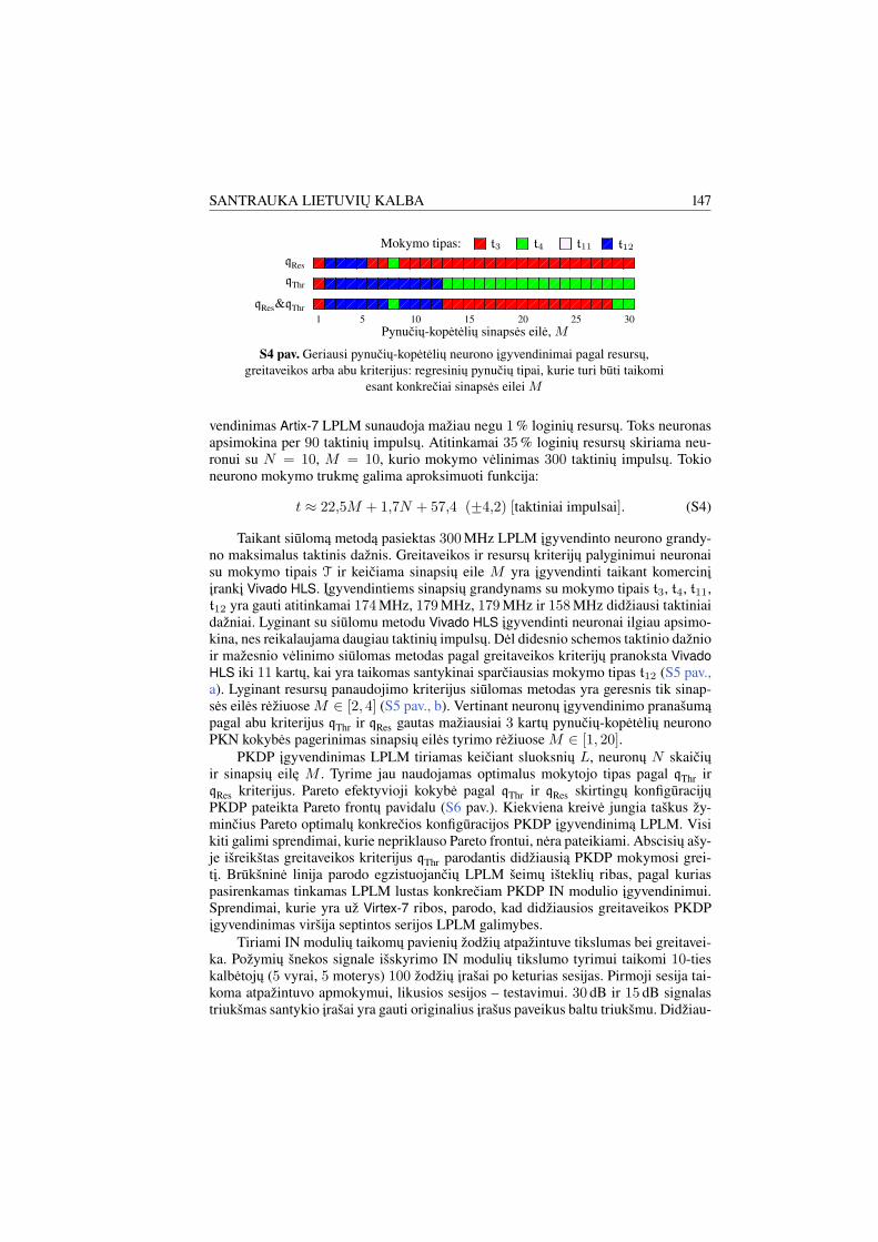
SANTRAUKA LIETUVIŲ KALBA 147
5 10 15 20 25 301
qRes
qThr
qRes&qThr
Pynučių-kopėtėlių sinapsės eilė, M
Mokymo tipas: t3 t4 t11 t12
S4 pav. Geriausi pynučių-kopėtėlių neurono įgyvendinimai pagal resursų,greitaveikos arba abu kriterijus: regresinių pynučių tipai, kurie turi būti taikomi
esant konkrečiai sinapsės eilei M
vendinimas Artix-7 LPLM sunaudoja mažiau negu 1% loginių resursų. Toks neuronasapsimokina per 90 taktinių impulsų. Atitinkamai 35% loginių resursų skiriama neu-ronui su N = 10, M = 10, kurio mokymo vėlinimas 300 taktinių impulsų. Tokioneurono mokymo trukmę galima aproksimuoti funkcija:
t ≈ 22,5M + 1,7N + 57,4 (+−4,2) [taktiniai impulsai]. (S4)
Taikant siūlomą metodą pasiektas 300MHz LPLM įgyvendinto neurono grandy-no maksimalus taktinis dažnis. Greitaveikos ir resursų kriterijų palyginimui neuronaisu mokymo tipais T ir keičiama sinapsių eile M yra įgyvendinti taikant komercinįįrankį Vivado HLS. Įgyvendintiems sinapsių grandynams su mokymo tipais t3, t4, t11,t12 yra gauti atitinkamai 174MHz, 179MHz, 179MHz ir 158MHz didžiausi taktiniaidažniai. Lyginant su siūlomu metodu Vivado HLS įgyvendinti neuronai ilgiau apsimo-kina, nes reikalaujama daugiau taktinių impulsų. Dėl didesnio schemos taktinio dažnioir mažesnio vėlinimo siūlomas metodas pagal greitaveikos kriterijų pranoksta VivadoHLS iki 11 kartų, kai yra taikomas santykinai sparčiausias mokymo tipas t12 (S5 pav.,a). Lyginant resursų panaudojimo kriterijus siūlomas metodas yra geresnis tik sinap-sės eilės rėžiuose M ∈ [2, 4] (S5 pav., b). Vertinant neuronų įgyvendinimo pranašumąpagal abu kriterijus qThr ir qRes gautas mažiausiai 3 kartų pynučių-kopėtėlių neuronoPKN kokybės pagerinimas sinapsių eilės tyrimo rėžiuose M ∈ [1, 20].
PKDP įgyvendinimas LPLM tiriamas keičiant sluoksnių L, neuronų N skaičiųir sinapsių eilę M . Tyrime jau naudojamas optimalus mokytojo tipas pagal qThr irqRes kriterijus. Pareto efektyvioji kokybė pagal qThr ir qRes skirtingų konfigūracijųPKDP pateikta Pareto frontų pavidalu (S6 pav.). Kiekviena kreivė jungia taškus žy-minčius Pareto optimalų konkrečios konfigūracijos PKDP įgyvendinimą LPLM. Visikiti galimi sprendimai, kurie nepriklauso Pareto frontui, nėra pateikiami. Abscisių ašy-je išreikštas greitaveikos kriterijus qThr parodantis didžiausią PKDP mokymosi grei-tį. Brūkšninė linija parodo egzistuojančių LPLM šeimų išteklių ribas, pagal kuriaspasirenkamas tinkamas LPLM lustas konkrečiam PKDP IN modulio įgyvendinimui.Sprendimai, kurie yra už Virtex-7 ribos, parodo, kad didžiausios greitaveikos PKDPįgyvendinimas viršija septintos serijos LPLM galimybes.
Tiriami IN modulių taikomų pavienių žodžių atpažintuve tikslumas bei greitavei-ka. Požymių šnekos signale išskyrimo IN modulių tikslumo tyrimui taikomi 10-tieskalbėtojų (5 vyrai, 5 moterys) 100 žodžių įrašai po keturias sesijas. Pirmoji sesija tai-koma atpažintuvo apmokymui, likusios sesijos – testavimui. 30 dB ir 15 dB signalastriukšmas santykio įrašai yra gauti originalius įrašus paveikus baltu triukšmu. Didžiau-
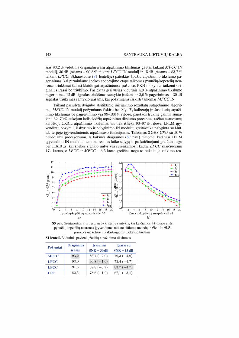
148 SANTRAUKA LIETUVIŲ KALBA
sias 93,2% vidutinis originalių įrašų atpažinimo tikslumas gautas taikant MFCC INmodulį, 30 dB įrašams – 90,8% taikant LFCC IN modulį ir 15 dB įrašams – 83,7%taikant LPCC. Skliaustuose (S1 lentelėje) pateiktas žodžių atpažinimo tikslumo pa-gerinimas, kai pirminiame šnekos apdorojimo etape taikomas pynučių-kopėtėlių neu-ronas triukšmui šalinti klaidingai atpažintuose įrašuose. PKN mokymui taikomi ori-ginalūs įrašai be triukšmo. Pasiektas geriausias vidutinis 4,9% atpažinimo tikslumopagerinimas 15 dB signalas triukšmas santykio įrašams ir 2,0% pagerinimas – 30 dBsignalas triukšmas santykio įrašams, kai požymiams išskirti taikomas MFCC IN.
Taikant pasiūlytą dvigubo atsitiktinio inicijavimo rezultatų sutapdinimo algorit-mą, MFCC IN modulį požymiams išskirti bei M1, F4 kalbėtojų įrašus, kurių atpaži-nimo tikslumas be pagreitinimo yra 99–100% ribose, paieškos trukmę galima suma-žinti 62–70% aukojant kelis žodžių atpažinimo tikslumo procentus, tačiau testuojamųkalbėtojų žodžių atpažinimo tikslumas vis tiek išlieka 90–97% ribose. LPLM įgy-vendintų požymių išskyrimo ir palyginimo IN modulių greitaveika palyginta su Mat-lab terpėje įgyvendintomis atpažintuvo funkcijomis. Taikomas 3GHz CPU su 50%naudojamu procesoriumi. Iš laikinės diagramos (S7 pav.) matoma, kad visi LPLMįgyvendinti IN moduliai tenkina realaus laiko sąlygą ir paskaičiuojami greičiau neguper 11610µs, kai šnekos signalo imtys yra surenkamos į kadrą. LFCC skaičiuojami174 kartus, o LPCC ir MFCC – 3,5 karto greičiau negu to reikalauja veikimo rea-
0 2 4 6 8 10 12 14 16 18 203
4
5
6
7
8
9
10
11
12
t3t4t11t12
q⋆ T
hr/q
HL
ST
hr[k
arta
i]
Pynučių-kopėtėlių sinapsės eilė M
a)
0 2 4 6 8 10 12 14 16 18 200,4
0,5
0,6
0,7
0,8
0,9
1
1,1
t3t4t11t12
q⋆ R
es/q
HL
SR
es[k
arta
i]
Pynučių-kopėtėlių sinapsės eilė M
b)
S5 pav. Greitaveikos a) ir resursų b) kriterijų santykis, kai keičiamos M -tosios eilėspynučių-kopėtėlių neuronas įgyvendintas taikant siūlomą metodą ir Vivado HLS
įrankį esant keturiems skirtingiems mokymo būdams
S1 lentelė. Vidutinis pavienių žodžių atpažinimo tikslumas
PožymiaiOriginalūs Įrašai su Įrašai su
įrašai SNR = 30 dB SNR = 15 dB
MFCC 93,2 86,7 (+2,0) 79,3 (+4,9)
LFCC 93,0 90,8 (+1,0) 72,4 (+4,7)
LPCC 91,5 89,8 (+0,7) 83,7 (+4,7)
LPC 82,5 78,6 (+1,2) 67,1 (+3,1)
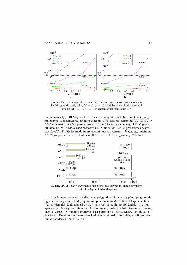
SANTRAUKA LIETUVIŲ KALBA 149
0 0,2 0,4 0,6 0,8 1 1,20
0,5
1
1,5
2
2,5
Artix−7
Kintex−7
Virtex−7
L = 2
L = 5
L = 10
L = 20
×106
q−1
Res
qThr [MHz]
a)
0 0,2 0,4 0,6 0,8 1 1,20
0,5
1
1,5
2
2,5
Artix−7
Kintex−7
Virtex−7
N = 2
N = 5
N = 10
N = 20
×106
q−1
Res
qThr [MHz]
b)
S6 pav. Pareto fronto priklausomybė nuo resursų ir spartos kriterijų konkrečiamPKDP įgyvendinimui, kai a) M = 10, N = 10 ir keičiamas sluoksnių skaičius L
arba kai b) L = 10, M = 10 ir keičiamas neuronų skaičius N
liuoju laiku sąlyga. DLSKc per 11610µs spėja palyginti ištartą žodį su 90 įrašų saugo-mų žodyne. Dėl santykinai 30 kartų didesnio CPU taktinio dažnio MFCC, LPCC irLPC požymiai paskaičiuojami atitinkamai 10 ir 5 kartus greičiau negu LPLM įgyven-dintame 100MHz MicroBlaze procesoriaus IN modulyje. LPLM pranašumas pastebi-mas LFCC ir DLSK IN modulių įgyvendinimuose. Lyginant su Matlab įgyvendinimuLFCC yra paspartintas 1,5 kartus, o DLSK ir DLSKc – daugiau negu 280 kartų.
LPLMCPU
MFCC
LPCC
LPC
LFCC
DLSK
DLSKc
3304µs285µs
3349µs313µs
1667µs307µs
66µs102µs
333µs 94100µs
128µs 36320µs
11610µs
Veikimorealiuoju laiku
riba
0 1000 5000 10000 t [µs]
S7 pav. LPLM ir CPU įgyvendintų intelektinės nuosavybės modulių požymiamsišskirti ir palyginti laikinė diagrama
Atpažintuvo greitaveika ir tikslumas palyginti su kitų autorių pilnai programiniuįgyvendinimu grįstu LPLM programiniu procesoriumi MicroBlaze. Eksperimentai at-likti su vienodais žodynais: (5 vyrai, 5 moterys) 10 sesijų po 100 žodžių, 4 sesijos –apmokymui, 6 sesijos – testavimui. Atsižvelgiant į skirtingus diskretizavimo ir taktinįdažnius LFCC IN modulio greitaveika paspartinta 320 kartų, DLSKc IN modulio –348 kartus. Dėl didesnio šnekos signalo diskretizavimo dažnio žodžių atpažinimo tiks-lumas padidėjo 4,9% iki 97,7%.

150 SANTRAUKA LIETUVIŲ KALBA
Bendrosios išvados
Disertacijoje pasiūlyti sprendimai pynučių-kopėtėlių daugiasluoksnio perceptronų in-telektinės nuosavybės (PKDP IN) moduliams įgyvendinti lauku programuojama logi-ne matrica (LPLM) ir ištirtas modulių efektyvumas juos taikant neįgaliesiems skirta-me lietuvių šnekos atpažintuve. Gauti šie elektros ir elektronikos inžinerijos mokslokrypčiai svarbūs rezultatai:
1. Sukurtas ir eksperimentiškai patvirtintas efektyvus metodas PKDP įgyven-dinti LPLM:
1.1. Sukurtas PKDP kompiliatorius generuoja daugiau nei 3 kartus efektyves-nį IN modulį lyginant su komerciniu Vivado HLS įrankiu.
1.2. Sukurtas neurono apdorojimo elementas, grįstas LPLM DSP bloko struk-tūra, yra optimizuotas greitaveikai, jis vėlina tik 7 taktiniais impulsais,garantuojant mažesnę nei 1% vidutinę absoliučią išėjimo signalo klai-dą ir 1,8×10⁻³ šaknies vidutinė kvadratinę pynučių-kopėtėlių neuronoperdavimo funkcijos klaidą.
1.3. Eksperimentiniais tyrimais išgautos žinios apie greičiausius PKDP mo-kymo algoritmus ir jų geriausias regresines pynutes T ∈ {t3, t4, t11, t12}pritaikytos minimizuojant peržvalgos lentelių skaičių ir vėlinimą.
2. Įgyvendinimams vertinti pasiūlytas PKDP grandynų sintezės specializuotųkriterijų Pareto frontų skaičiavimo būdas:
2.1. Atrinktas LPLM lustas yra optimalus pagal reikalavimus PKDP struktū-rai, diskretizavimo dažnį ir kitus resursus.
2.2. Įgyvendintos dvi optimizavimo strategijos: greitaveikai ir resursams.
3. Neįgaliesiems skirtame lietuvių šnekos atpažintuve įgyvendinti ir eksperi-mentiškai patikrinti optimizuoti LPLM IN moduliai:
3.1. Pynučių-kopėtėlių neurono IN modulio taikymas 4% padidina atpažini-mo tikslumą esant 15 dB signalas triukšmas santykiui.
3.2. Žodžiams įrašuose be triukšmo atpažinti tinka MFCC ir LFCC IN mo-duliai.
3.3. LFCC ir LPCC IN moduliai taikytini esant 30 dB signalo ir triukšmosantykiui, o esant 15 dB – LPCC IN modulis užtikrina didžiausią atpaži-nimo tikslumą.
4. Sukurtas ir patikrintas pirmasis neįgaliesiems skirto valdymo lietuviška šne-ka įrenginio, grįsto LPLM, prototipas:
4.1. Naujas spartesnis žodžių sutapdinimo algoritmas naudoja apribotą dina-minį laiko skalės kraipymą ir atpažįsta žodžius 2,6 karto greičiau, nepra-rasdamas 97% siekiančio atpažinimo tikslumo.
4.2. Pasiūlytas dvigubo atsitiktinio iniciavimo rezultatų sutapdinimo algorit-mas papildomai iki 2,6 karto paspartina atpažinimo procesą, tačiau su-mažina iki 90% žodžių atpažinimo tikslumą.
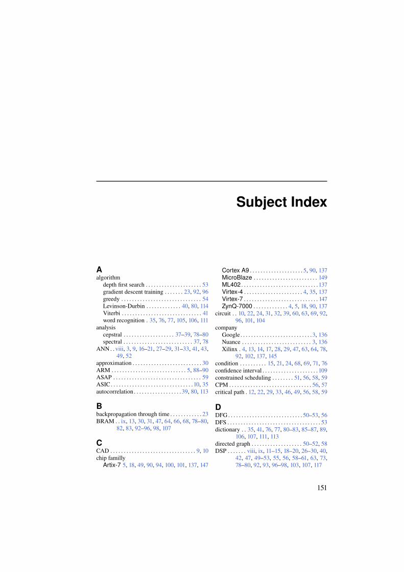
Subject Index
Aalgorithm
depth first search . . . . . . . . . . . . . . . . . . . . . 53gradient descent training . . . . . . . 23, 92, 96greedy . . . . . . . . . . . . . . . . . . . . . . . . . . . . . . 54Levinson-Durbin . . . . . . . . . . . . . 40, 80, 114Viterbi . . . . . . . . . . . . . . . . . . . . . . . . . . . . . . 41word recognition . 35, 76, 77, 105, 106, 111
analysiscepstral . . . . . . . . . . . . . . . . . . . 37–39, 78–80spectral . . . . . . . . . . . . . . . . . . . . . . . . . . 37, 78
ANN . . viii, 3, 9, 16–21, 27–29, 31–33, 41, 43,49, 52
approximation . . . . . . . . . . . . . . . . . . . . . . . . . . 30ARM . . . . . . . . . . . . . . . . . . . . . . . . . . . . 5, 88–90ASAP . . . . . . . . . . . . . . . . . . . . . . . . . . . . . . . . . 59ASIC. . . . . . . . . . . . . . . . . . . . . . . . . . . . . . . 10, 35autocorrelation . . . . . . . . . . . . . . . . . . 39, 80, 113
Bbackpropagation through time . . . . . . . . . . . . 23BRAM . . ix, 13, 30, 31, 47, 64, 66, 68, 78–80,
82, 83, 92–96, 98, 107
CCAD . . . . . . . . . . . . . . . . . . . . . . . . . . . . . . . . 9, 10chip familly
Artix-7 5, 18, 49, 90, 94, 100, 101, 137, 147
Cortex A9 . . . . . . . . . . . . . . . . . . . . 5, 90, 137MicroBlaze . . . . . . . . . . . . . . . . . . . . . . . . 149ML402 . . . . . . . . . . . . . . . . . . . . . . . . . . . . . 137Virtex-4 . . . . . . . . . . . . . . . . . . . . . . 4, 35, 137Virtex-7 . . . . . . . . . . . . . . . . . . . . . . . . . . . . 147ZynQ-7000 . . . . . . . . . . . . . 4, 5, 18, 90, 137
circuit . . 10, 22, 24, 31, 32, 39, 60, 63, 69, 92,96, 101, 104
companyGoogle . . . . . . . . . . . . . . . . . . . . . . . . . . .3, 136Nuance . . . . . . . . . . . . . . . . . . . . . . . . . . 3, 136Xilinx . 4, 13, 14, 17, 28, 29, 47, 63, 64, 78,
92, 102, 137, 145condition . . . . . . . . . . 15, 21, 24, 68, 69, 71, 76confidence interval . . . . . . . . . . . . . . . . . . . . . 109constrained scheduling . . . . . . . . 51, 56, 58, 59CPM . . . . . . . . . . . . . . . . . . . . . . . . . . . . . . . 56, 57critical path . 12, 22, 29, 33, 46, 49, 56, 58, 59
DDFG . . . . . . . . . . . . . . . . . . . . . . . . . . . . 50–53, 56DFS . . . . . . . . . . . . . . . . . . . . . . . . . . . . . . . . . . . 53dictionary . . 35, 41, 76, 77, 80–83, 85–87, 89,
106, 107, 111, 113directed graph . . . . . . . . . . . . . . . . . . . 50–52, 58DSP . . . . . . . viii, ix, 11–15, 18–20, 26–30, 40,
42, 47, 49–53, 55, 56, 58–61, 63, 73,78–80, 92, 93, 96–98, 103, 107, 117
151
152 SUBJECT INDEX
DTW. . . . . .41, 42, 75, 78–81, 83–86, 90, 107,111–115, 118
Eefficient implementation . . . 32, 46, 48–50, 73,
103
Ffeatures
classification . . . . . 41, 42, 81, 106, 108, 109extraction . . . . . . . 34, 78, 105, 108, 110, 113selection . . . . . . . . . . . . . . . . . . . . . . 78, 85, 86vector . . . . . . . . . . . . . . . . . 77, 83, 85, 86, 111
FFT . . . . . . . . . . . . . . . . . . . . . . . . . . . . . . 106, 113filter . . . . . . . . . . . . . . . . . . 14, 16, 17, 21, 22, 39
band-pass . . . . . . . . . . . . . . . . . . . . . . . . 21, 63band-stop . . . . . . . . . . . . . . . . . . . . . . . . . . . . 67stability . . . . . . . . . . . . . . . . . . . . . . . . . . 21–23
FIR . . . . . . . . . . . . . . . . . . . . . . . . . . . . . . . . 14, 16FPGA . . . . . . . . . . . . . . . . . . v, ix, 1, 3–6, 8–20,
26–33, 35, 36, 38, 39, 41–43, 46–52,56, 63, 68–71, 73, 75–78, 81, 88–94,96, 98–108, 113, 116–118
clock frequency . 22, 29, 33, 46, 48, 61, 73,90, 102, 106, 107, 113
FPGA resourceBRAM. . .11, 12, 30, 47, 63, 66, 77, 78, 80,
82, 93, 95, 98, 107DSP. .11, 12, 29, 47, 49, 53, 58, 60, 78, 80,
93, 96, 97, 107LUT . . . 11, 12, 30, 47, 51, 93, 98, 100, 107LUT equivalent . . . . . . . . . . . . . . . . . . . . . 104Slice . . . . . . . . . . . . . . . . . . . . . . . . . . . . . 11, 12
functionactivation . . . . . . . . . . . 29, 51, 60, 66, 93, 95Hanning . . . . . . . . . . . . . . . . . . . . . . . . . 76, 114trigonometric . . . . . . . . . . . . . . . . . 51, 60, 64window . . . . . . . . 39, 76, 78, 82, 84, 87, 114
Ggraph . . . . . . . . . . . . . . . . . . . . . . . . 50, 51, 53, 55
covering . . . . . . . . . . . . . . . . . . . 51, 54, 56, 59isomorphism. . . . . . . . . . . . . . . . . . . . . . . . . 53matching . . . . . . . . . . . . . . . . . . . . . 51, 53, 54merging . . . . . . . . . . . . . . . . . . . . . . 51, 54, 56
HHDL . . . . . . . 10, 14, 17, 18, 32, 50, 59–61, 102hidden Markov model . . . . . . . . . . . . . . . . 34, 41HLS . . . . . . . . . . . . . . . . . . 10, 11, 14, 15, 18, 42
IIIR . . . . . . . . . . . . . . . . . . . . . . . . . . . . . . . . . . . . 16implementation
criteria . . . . . . . . . . 33, 46, 48, 100, 102–104parallel . . 16, 19, 25, 33, 35, 41, 42, 62, 68,
71, 80–82, 102pipeline . . 35, 49, 51, 55, 58, 61, 62, 71, 81,
83quality . . . . . . . . . . . . . . . . . . . . . . . 33, 46, 48strategy . . 45, 46, 48, 53, 59, 63, 68, 71, 73,
117instruction
modification . . . . . . . . . . . . . . . . . . 55, 60, 61scheduling . . . . . . 13, 50, 56, 58, 59, 63, 73
investigation 61, 63, 92, 94, 96, 103, 104, 106,111
IP . . . . . . . . . . . . . . . . . . . . v, 3–6, 14, 17, 28, 38,43, 73, 75, 76, 78, 80, 81, 88–92, 102,106, 108, 110, 111, 115, 118
IP moduleautocorrelation . . . . . . . . . . . . . . . 39, 80, 114autoregression . . . . . . . . . . . . . . . . 39, 80, 114DTW . . 41, 77, 78, 81, 83, 85, 86, 107, 111,
113–115FFT . . . . . . . . . . . . . . . . . . . . . 78, 79, 113, 114framing . . . . . . . . . . . . . . . . . . . . . . . . . . 76, 79infrared . . . . . . . . . . . . . . . . . . . . . . . . . . 89, 90iterative voice response . . . . . . . . . . . . . . . 88LFCC . . . 37, 77, 78, 90, 106, 108, 113–115logarithm . . . . . . . . . . . . . . . . 78, 79, 113, 114LPC . . . . . . . . . 39, 78, 80, 90, 108, 113–115LPCC . . . . . . . . 39, 78, 80, 90, 108, 113–115MFCC . . . 38, 77–79, 90, 108, 109, 113–115MicroBlaze . . . . . . . . . . 35, 77, 80, 144, 145neuron processing element . .46, 51, 60–63,
71, 102, 104synchronization . . . . . . . . . . . . . . . 58, 76, 83UART. . . . . . . . . . . . . . . . . . . . . . . . . . . . . . . 90voice activity detector . . . . . . . . . . . . . . . . 89windowing . . . . . . . . . . . . . . . .39, 76–78, 114Zigbee . . . . . . . . . . . . . . . . . . . . . . . . . . . 89, 90
Llatency . . 12, 14, 19, 28–30, 32, 45–47, 49, 50,
54, 56, 58, 61, 64, 68–73, 78, 83, 98,100, 102, 103, 115
LFCC . . viii, 36–38, 78, 79, 90, 106–108, 111,113–115, 118
LL . . . . . . . . . . . . . . . . . . . . . . . . . . . . . . . . . 16, 68LLF. .17, 18, 21–24, 26, 49, 61, 92, 93, 96, 97

SUBJECT INDEX 153
LLMLP . v, ix, 3–6, 11, 12, 16, 22, 24–27, 42,43, 45–53, 55, 56, 61, 63, 68–73, 75,77, 91, 92, 96, 98, 103–105, 116, 117
LLN . ix, 21, 49, 62, 64, 66–68, 91–93, 95–98,100–103, 106, 110, 111, 115, 118
LPC . viii, 36, 37, 39–41, 78, 80, 90, 108, 111,113
LPCC viii, 36, 37, 39–41, 78, 80, 90, 108, 111,113–115, 118
LSR . . . . . . . . . . . . . . . 75, 88, 90, 105, 106, 108LUT . 11, 13, 18, 29–31, 33, 38, 39, 47, 52, 64,
66, 67, 92–95, 98, 100, 102, 103, 105,108, 115, 117
MMAC . . . . . . . . . . . . . . . . . . . . . . . . . . . 28, 29, 39MAE . . . . . . . . . . . . . . . . . . . . . . . viii, 65, 67, 93MFCC . . . . . . viii, 36–39, 78, 79, 90, 108, 111,
113–115, 118MLP . . . . . . . . . . . . . . . . . . . . . 16, 19, 22, 28, 29MME. . . . . . . . . . . . . . . . . . . . . . . . . . . . . .viii, 67model . . . . . . . . . . . . . . . . . . . . . . . 19, 34, 39, 41multilayer perceptron . . 16, 23, 25, 63, 68, 71,
104
Nnoise . . . . . . . . . . . . . . . . 15, 35, 75, 92, 108–110NPE . . . . . . . . . 45, 46, 60–63, 71, 72, 102, 105
Ooptimization strategy . . . . . . . . . . . . . 63, 68, 71order recursion . . . . . . . . . . . . . . . . . . . . . . . . . 23
PPAR . . . . . . . . . . . . . . . . . . 11, 28, 32, 33, 46, 61parameters . . 21, 23, 25, 28, 63, 64, 67, 71, 87,
92, 93, 111Pareto frontier . . . 45, 48, 73, 92, 103, 104, 115pattern matching . . . . . . . . .81, 85, 86, 111, 112power spectral density . . . . . . . . . . . . . . . . . . . 67precision . . . . . . . . . . . . . . . . . . . . . . . . . . . . . . . 19
fixed-point13, 14, 16, 28, 39, 41, 47, 49, 63,65, 66, 92
floating-point 14, 16, 41, 47, 49, 63, 66, 77,78, 106
programming languageC . . . . . . . . . . . . . . . . . . . . . . . . . 10, 15, 28, 42C++ . . . . . . . . . . . . . . . . . . . . . . . . . . . . . 15, 28C# . . . . . . . . . . . . . . . . . . . . . . . . . . . . . . . . . . 28Matlab . . . . . . . . . . . . . . . . . . . . . . . . . . . . . . 28
RTL . . . . . . . . . . . . . . . . . . . . . . . . . . . . . . . . 28SystemC . . . . . . . . . . . . . . . . . . . . . . . . . 10, 15Verilog . . . . . . . . . . . . . . . . . . . . . . . . . . . 10, 18VHDL . . . . . . . . . vii, 10, 18, 28, 42, 96, 144
PWL . . . . . . . . . . . . . . . . . . . . . . . . . . . . . . . 29, 30
Qquality criteria . . . . . . . . . . . . . . 32, 45, 46, 102
RRAM . . . . . . . . . . 11–13, 30, 33, 47, 61, 73, 115real-time . . 35–39, 42, 76, 77, 81, 85, 113, 114reconfigurable block . . . . 18, 29, 31, 49, 52, 55regressor lattice .24, 25, 49, 51, 56, 61, 62, 98,
100, 102, 103, 115RMSE . . . . . . . . . . . . . . . . . . . . . . . . . . . . . viii, 95ROM . . . . . . . . . . . . . . . . . . . . . . . . . . . 13, 18, 60RTL . . . . . . . . . . . . . . . . . . . . . . . . . 10–12, 14, 29
SSchur recursion . . . . . . . . . . . . . . . . . . . . . . . . . 21software
AccelDSP . . . . . . . . . . . . . . . . . . . . . . . 14, 15C-to-Silicon . . . . . . . . . . . . . . . . . . . . . . 14, 15Catapult C . . . . . . . . . . . . . . . . . . . . . . . 14, 15HDL Coder . . . . . . . . . . . . . . . . . . . . . . 14, 15HLS . . . . . . . . . . . . . . . . . . . . . . . . . . . . . . . . 96ISE Design Suite . . . . 4, 14, 101, 102, 137LabView . . . . . . . . . . . . . . . . . 10, 15, 39, 140Matlab . .4, 10, 14, 28, 63, 64, 67, 113, 137,
144, 148, 149ModelSim . . . . . . . . . . . . . . . . . . . . . . . 4, 137RapidSmith . . . . . . . . . . . . . . . . . . . . . . . . . 11Simulink . . . . . . . . . . 10, 14, 19, 28, 39, 140StateCAD . . . . . . . . . . . . . . . . . . . . . . . 14, 15Synphony . . . . . . . . . . . . . . . . . . . . . . . 14, 15System Generator . . . . . . . . . . . . . . . 14, 63Verilog . . . . . . . . . . . . . . . . . . . . . . . . . . . . . 140VHDL . . . . . . . . . . . . . . . . . . . . . . . . . . . . . .140Vivado HLS . . 4, 5, 14, 15, 64, 67, 92, 102,
103, 116, 117, 137, 138, 140, 144, 147,148, 150
XSG . . . . . . . . . . . . . . . . . . . . . . . . . . . . . 14, 15speech recognition. . . .34, 41, 76, 81, 105, 113speech records . . . . . 76, 88, 105, 107–109, 111structure.10, 12, 16–19, 21, 28, 32, 48, 50, 63,
68, 71subgraph . . . . . . . . . 50, 53–55, 59, 60, 96, 103
elimination . . . . . . . . . . . . . . . . . . . . . . . . . . 54support vector machine . . . . . . . . . . . . . . . . . . 28

154 SUBJECT INDEX
synapse . 13, 19, 21, 22, 29, 31, 32, 46, 47, 49,55, 56, 61–63, 66, 68, 71, 92, 96, 98,100–103, 110
systolic array. . . . . . . . . . . . . . . . . . . . .31, 40, 41
Tthreshold . . . . . . . . . . . . . . . . . . . . . . . . . . . . . . . 19transfer function . . . . . . . . . . . . . . . . . 67, 95, 96
Uuser interface . . . . . . . . . . . . . . . . . . . . . . . . . . . 88
Vvector35, 37–39, 41, 42, 57, 63, 77, 81, 83, 85,
86, 111VLSI . . . . . . . . . . . . . . . . . . . . . . . . . . . . . . . . . . 31
Zzero-pole plane . . . . . . . . . . . . . . . . . . . . . . . . . 93

Annexes
Annex A. Created Intellectual Property Cores
Annex B. The Co-authors’ Agreement to PresentPublications Material in the Dissertation
Annex C. The Copies of Scientific Publications bythe Author on the Topic of theDissertation
4The annexes are supplied in the enclosed compact disc
155
4

Tomyslav SLEDEVIČ
AN EFFICIENT IMPLEMENTATION OF LATTICE-LADDER MULTILAYERPERCEPTRONS IN FIELD PROGRAMMABLE GATE ARRAYS
Doctoral Dissertation
Technological Sciences,Electrical and Electronic Engineering (01T)
PYNUČIŲ-KOPĖTĖLIŲ DAUGIASLUOKSNIŲ PERCEPTRONŲ EFEKTYVUSĮGYVENDINIMAS LAUKU PROGRAMUOJAMOMIS LOGINĖMIS MATRICOMIS
Daktaro disertacija
Technologijos mokslai,elektros ir elektronikos inžinerija (01T)
2016 05 06. 14,25 sp. l. Tiražas 20 egz.
Vilniaus Gedimino technikos universiteto leidykla „Technika“,
Saulėtekio al. 11, LT-10223 Vilnius,
http://leidykla.vgtu.lt
Spausdino BĮ UAB „Baltijos kopija“,
Kareivių g. 13B, LT-09109 Vilnius