HAL Id: hal-02362102https://hal.archives-ouvertes.fr/hal-02362102

Submitted on 18 Nov 2019

HAL is a multi-disciplinary open accessarchive for the deposit and dissemination of sci-entific research documents, whether they are pub-lished or not. The documents may come fromteaching and research institutions in France orabroad, or from public or private research centers.

L’archive ouverte pluridisciplinaire HAL, estdestinée au dépôt et à la diffusion de documentsscientifiques de niveau recherche, publiés ou non,émanant des établissements d’enseignement et derecherche français ou étrangers, des laboratoirespublics ou privés.

An Efficient Parametric Linear Programming Solver andApplication to Polyhedral Projection

Hang Yu, David Monniaux

To cite this version:Hang Yu, David Monniaux. An Efficient Parametric Linear Programming Solver and Applicationto Polyhedral Projection. Static Analysis (SAS 2019), Oct 2019, Porto, Portugal. pp.203-224,�10.1007/978-3-030-32304-2_11�. �hal-02362102�

An efficient parametric linear programming solver

and application to polyhedral projection

Hang Yu and David Monniaux

Univ. Grenoble Alpes, CNRS, Grenoble INP∗

F-38000 Grenoble, France

First-name.Last-name@univ-grenoble-alpes.fr

October 8, 2019

Abstract

Polyhedral projection is a main operation of the polyhedron abstractdomain. It can be computed via parametric linear programming (PLP),which is more efficient than the classic Fourier-Motzkin elimination method.

In prior work, PLP was done in arbitrary precision rational arithmetic.In this paper, we present an approach where most of the computationis performed in floating-point arithmetic, then exact rational results arereconstructed.

We also propose a workaround for a difficulty that plagued previous at-tempts at using PLP for computations on polyhedra: in general the linearprogramming problems are degenerate, resulting in redundant computa-tions and geometric descriptions.

1 Introduction and related work

Abstract interpretation [6] is an approach for obtaining invariant properties ofprograms, which may be used to verify their correctness. Abstract interpre-tation searches for invariants within an abstract domain. For numerical prop-erties, a common and cheap choice is one interval per variable per location inthe program, but this cannot represent relationships between variables. Suchimprecision often makes it impossible to prove properties of the program usingthat domain. If we retain linear equalities and inequalities between variables,we obtain the domain of convex polyhedra [7], which is more expensive, but moreprecise.

∗Institute of Engineering Univ. Grenoble Alpes

1

Several implementations of the domain of convex polyhedra over the fieldof rational numbers are available. The most popular ones for abstract inter-pretation are NewPolka1 and the Parma Polyhedra Library (PPL) [1]. Theselibraries, and others, use the double description of polyhedra: as generators(vertices, and for unbounded polyhedra, rays and lines) and constraints (linearequalities and inequalities). Some operations are easier on one representationthan on the other, and some, such as removing redundant constraints or gen-erators, are easier if both are available. One representation is computed fromthe other using Chernikova’s algorithm [4, 16]. This algorithm is expensive insome cases, and, furthermore, in some cases, one representation is exponentiallylarger than the other. This is in particular the case of the generator repre-sentation of hypercubes or, more generally, products of intervals; thus intervalanalysis which simulate using convex polyhedra in the double description hascost exponential in the dimension.

In 2012 Verimag started implementing a library using constraints only, calledVPL (Verified Polyhedra Library) [11, 17]. There are several reasons for us-ing only constraints; we have already cited the high generator complexity ofsome polyhedra commonly found in abstract interpretation, and the high costof Chernikova’s algorithm. Another reason was to be able to certify the resultsof the computation, in particular that the obtained polyhedra includes the onethat should have been computed, which is the property that ensures the sound-ness of abstract interpretation. One can certify that each constraint is correctby exhibiting coefficients, as in Farkas’ lemma.

In the first version of VPL, all main operations boiled down to projection,performed using Fourier-Motzkin elimination [9], but this method generatesmany redundant constraints which must be eliminated at high cost. Also, forprojecting out many variables x1, . . . , xn, it computes all intermediate steps(projection of x1, then of x2. . . ), even though they may be unneeded and havehigh description complexity. In the second version, projection and convex hullboth boil down to parametric linear programming [14]. The current versionof VPL is based on a parametric linear programming solver implemented inarbitrary precision arithmetic in OCaml [18].

In this paper, we improved on this approach in two respects.

• We replace most of the exact computations in arbitrary precision rationalnumbers by floating-point computations performed using an off-the-shelflinear programming solver. We can however recover exact solutions andcheck them exactly, an approach that has previously been used for SMT-solving [20, 15].

• We resolve some difficulties due to geometric degeneracy in the problemsto be solved, which previously resulted in many redundant computations.

Furthermore, the solving is divided into independent tasks, which may be sched-uled in parallel. The parallel implementation is covered in [5].

1Now distributed as part of APRON http://apron.cri.ensmp.fr/library/

2

2 Notations and preliminaries

2.1 Notations

Capital letters (e.g. A) denote matrices, small bold letters (e.g. x) denotevectors, small letters (e.g. b) denote scalars. The ith row of A is ai•, its jthcolumn is a•j . P : Ax + b ≥ 0 denotes a polyhedron and C a constraint. Theith constraint of P is Ci: ai•x ≥ bi, where bi is the ith element of b. aij denotesthe element at the ith row and the jth column of A. Q denotes the field ofrational numbers, and F is the set of finite floating-point numbers, consideredas a subset of Q.

2.2 Linear programming

Linear programming (LP) consists in getting the optimal value of a linear func-tion Z(λ) subject to a set of linear constraints Aλ = b, λ ≥ 0 2, where λ is thevector of variables. The optimal value Z∗ is reached at λ∗: Z∗ = Z(λ∗).

2.3 Basic and non-basic variables

We use the implementation of the simplex algorithm in GLPK3 as LP solver.In the simplex algorithm each constraint is expressed in the form (λB)i =∑n

j=1aij(λN )j + ci, where (λB)i is known as a basic variable, the (λN )j is

non-basic variable, and ci is a constant. The basic variables constitute a basis.The basic and non-basic variables form a partition of the variables, and theobjective function is obtained by substituting the basic variables with non-basicvariables.

2.4 Parametric linear programming

A parametric linear program (PLP) is a linear program, subjecting to Aλ =b, λ ≥ 0, whose objective function Z(λ,x) contains parameters x appearinglinearly.4 The PLP reaches optimum at the vertex λ∗, and the optimal solutionis a set of (Ri, Z

∗

i (x)). Ri is the region of parameters x, in which the basis doesnot change. Z∗

i (x) is the optimal function corresponding toRi, meaning that allthe parameters in Ri will lead to the same optimal function Z∗

i (x). In the caseof primal degeneracy (Section 5), the optimal vertex λ∗ has multiple partitionsof basic and non-basic variables, thus an optimal function can be obtained bydifferent bases, i.e., several regions share the same optimal function.

2This is the canonical form of the LP problem. All the LP problems can be transformedinto this form.

3The GNU Linear Programming Toolkit (GLPK) is a linear programming solver imple-mented in floating-point arithmetic. https://www.gnu.org/software/glpk/

4There also exist parametric linear programs where the parameters are in the constantterms of the inequalities, we do not consider them here.

3

2.5 Redundant constraints

Definition 1 (Redundant). A constraint is said to be redundant if it can beremoved without changing the shape of the polyhedron.

In our algorithms, there are several steps at which redundant constraintsmust be removed, which we call minimization of the polyhedron. For instancewe have P = {C1 : x1 − 2x2 ≤ −2, C2 : −2x1 + x2 ≤ −1, C3 : x1 + x2 ≤ 8, C4 :−2x1 − 4x2 ≤ −7}, and C4 is a redundant constraint.

The redundancy can be tested by Farkas’ Lemma: a redundant constraintcan be expressed as the combination of some other constraints.

Theorem 1 (Farkas’ Lemma). Let A ∈ Rm×nA ∈ Rm×n and b ∈ Rmb ∈ Rm.Then exactly one of the following two statements is true:

• There exists an x ∈ Rn such that Ax = b and x ≥ 0.

• There exists a y ∈ Rm such that ATy ≥ 0 and bTy < 0.

It is easy to determine the redundant constraints using Farkas’ lemma, butin our case we have much more irredundant constraints than redundant ones, inwhich case using Farkas’ lemma is not efficient. A new minimization algorithmwhich can find out the irredundant constraints more efficiently is explained in[19].

3 Algorithm

As our PLP algorithm is implemented with mix of rational numbers and floating-point numbers, we will make explicit the type of data used in the algorithm. Inthe pseudo-code, we annotate data with (nametype), where name is the nameof data and type is either Q or/and F. Q× F means that the data is stored inboth rational and floating-point numbers.

Floating-point computations are imprecise, and thus the floating-point LPsolver may provide an incorrect answer: it may report that the problem is in-feasible whereas it is feasible, that it is feasible even though it is infeasible, andit may provide an “optimal” solution that is not truly optimal. What our ap-proach guarantees is that, whatever the errors committed by the floating-pointLP solvers, the polyhedron that we computed is a valid over-approximation: italways includes the polyhedron that should have been computed. Details willbe explained later in this section and in Section 4.

In this section we do not consider the degeneracy, which will be talked inSection 5.

3.1 Flow chart

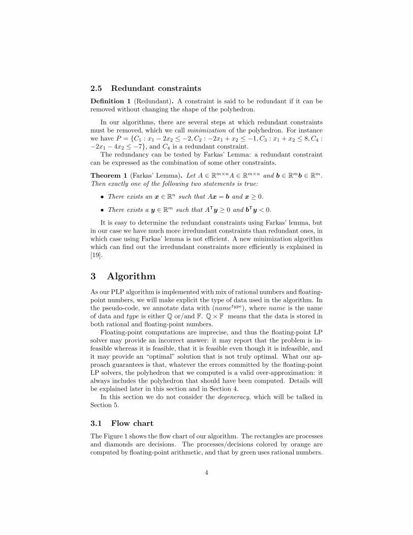
The Figure 1 shows the flow chart of our algorithm. The rectangles are processesand diamonds are decisions. The processes/decisions colored by orange arecomputed by floating-point arithmetic, and that by green uses rational numbers.

4

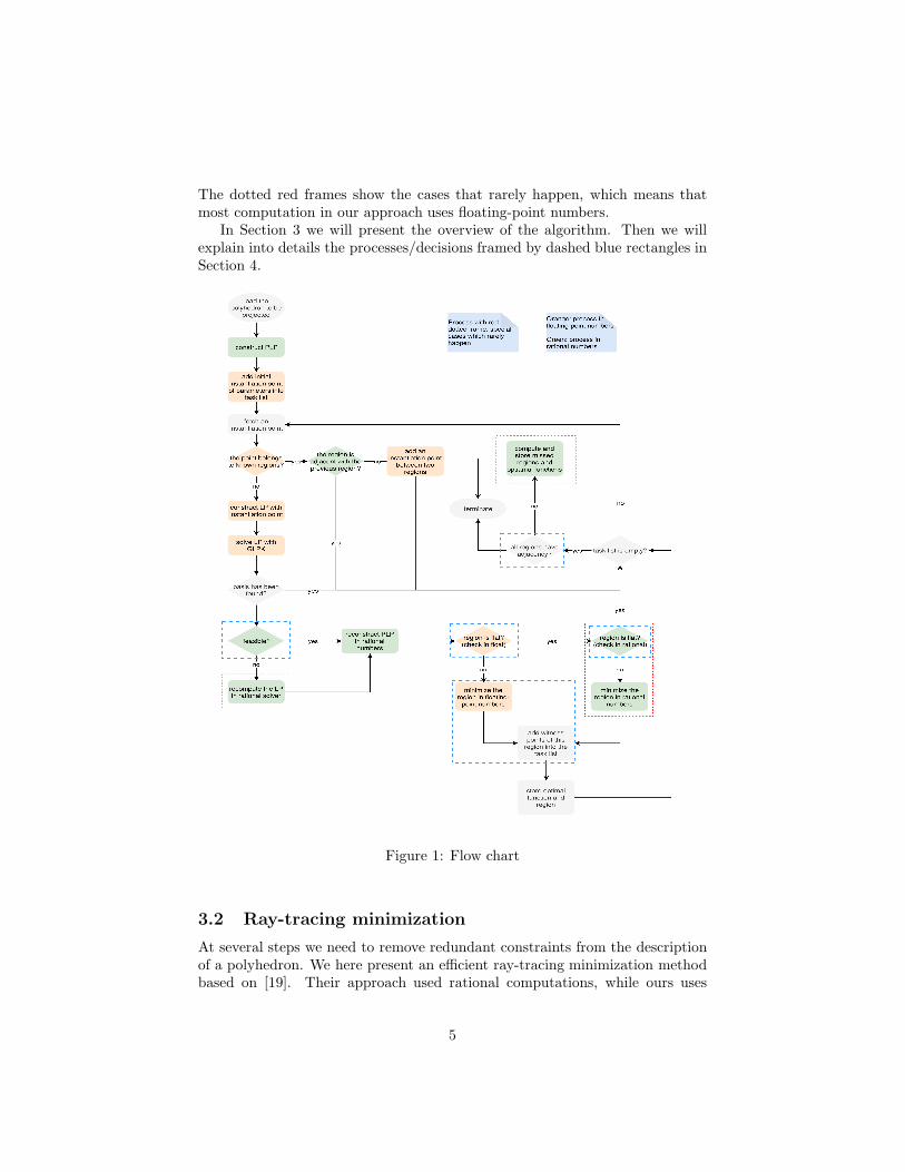
The dotted red frames show the cases that rarely happen, which means thatmost computation in our approach uses floating-point numbers.

In Section 3 we will present the overview of the algorithm. Then we willexplain into details the processes/decisions framed by dashed blue rectangles inSection 4.

Figure 1: Flow chart

3.2 Ray-tracing minimization

At several steps we need to remove redundant constraints from the descriptionof a polyhedron. We here present an efficient ray-tracing minimization methodbased on [19]. Their approach used rational computations, while ours uses

5

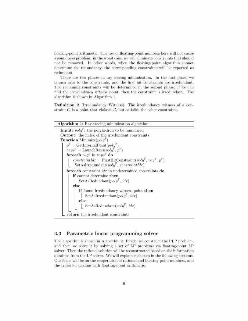
floating-point arithmetic. The use of floating-point numbers here will not causea soundness problem: in the worst case, we will eliminate constraints that shouldnot be removed. In other words, when the floating-point algorithm cannotdetermine the redundancy, the corresponding constraints will be reported asredundant.

There are two phases in ray-tracing minimization. In the first phase welaunch rays to the constraints, and the first hit constraints are irredundant.The remaining constraints will be determined in the second phase: if we canfind the irredundancy witness point, then the constraint is irredundant. Thealgorithm is shown in Algorithm 1.

Definition 2 (Irredundancy Witness). The irredundancy witness of a con-straint Ci is a point that violates Ci but satisfies the other constraints.

Algorithm 1: Ray-tracing minimization algorithm.

Input: polyF: the polyhedron to be minimizedOutput: the index of the irredundant constraintsFunction Minimize(polyF)

pF = GetInternalPoint(polyF)raysF = LaunchRays(polyF, pF)foreach rayF in raysF do

constraintIdx = FirstHitConstraint(polyF, rayF, pF)SetAsIrredundant(polyF, constraintIdx )

foreach constraint idx in undetermined constraints doif cannot determine then

SetAsRedundant(polyF, idx )else

if found irredundancy witness point then

SetAsIrredundant(polyF, idx )else

SetAsRedundant(polyF, idx )

return the irredundant constraints

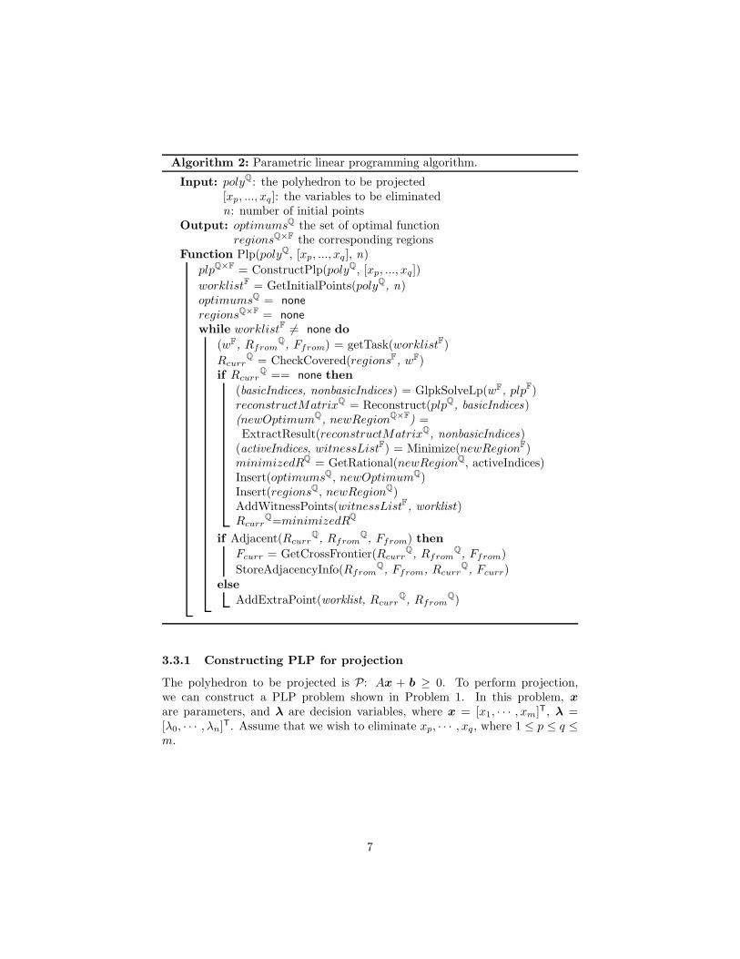
3.3 Parametric linear programming solver

The algorithm is shown in Algorithm 2. Firstly we construct the PLP problem,and then we solve it by solving a set of LP problems via floating-point LPsolver. Then the rational solution will be reconstructed based on the informationobtained from the LP solver. We will explain each step in the following sections.Our focus will be on the cooperation of rational and floating-point numbers, andthe tricks for dealing with floating-point arithmetic.

6

Algorithm 2: Parametric linear programming algorithm.

Input: polyQ: the polyhedron to be projected[xp, ..., xq]: the variables to be eliminatedn: number of initial points

Output: optimumsQ the set of optimal functionregionsQ×F the corresponding regions

Function Plp(polyQ, [xp, ..., xq], n)

plpQ×F = ConstructPlp(polyQ, [xp, ..., xq])

worklistF = GetInitialPoints(polyQ, n)optimumsQ = none

regionsQ×F = none

while worklistF 6= none do

(wF, RfromQ, Ffrom) = getTask(worklistF)

RcurrQ = CheckCovered(regionsF, wF)

if RcurrQ == none then

(basicIndices, nonbasicIndices) = GlpkSolveLp(wF, plpF)reconstructMatrixQ = Reconstruct(plpQ, basicIndices)(newOptimumQ, newRegionQ×F) =ExtractResult(reconstructMatrixQ, nonbasicIndices)(activeIndices, witnessListF) = Minimize(newRegionF)minimizedRQ = GetRational(newRegionQ, activeIndices)Insert(optimumsQ, newOptimumQ)Insert(regionsQ, newRegionQ)AddWitnessPoints(witnessListF, worklist)Rcurr

Q=minimizedRQ

if Adjacent(RcurrQ, Rfrom

Q, Ffrom) then

Fcurr = GetCrossFrontier(RcurrQ, Rfrom

Q, Ffrom)

StoreAdjacencyInfo(RfromQ, Ffrom, Rcurr

Q, Fcurr)else

AddExtraPoint(worklist, RcurrQ, Rfrom

Q)

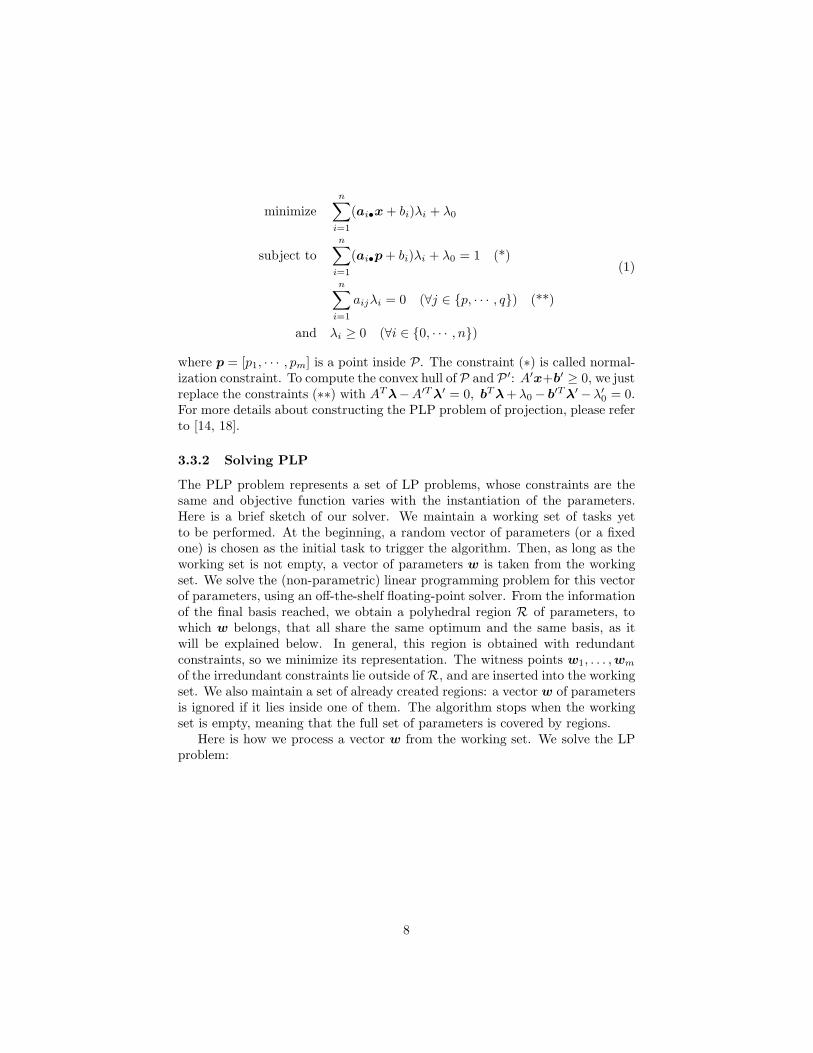
3.3.1 Constructing PLP for projection

The polyhedron to be projected is P: Ax + b ≥ 0. To perform projection,we can construct a PLP problem shown in Problem 1. In this problem, x

are parameters, and λ are decision variables, where x = [x1, · · · , xm]T, λ =[λ0, · · · , λn]

T. Assume that we wish to eliminate xp, · · · , xq, where 1 ≤ p ≤ q ≤m.

7

minimizen∑

i=1

(ai•x+ bi)λi + λ0

subject to

n∑

i=1

(ai•p+ bi)λi + λ0 = 1 (*)

n∑

i=1

aijλi = 0 (∀j ∈ {p, · · · , q}) (**)

and λi ≥ 0 (∀i ∈ {0, · · · , n})

(1)

where p = [p1, · · · , pm] is a point inside P. The constraint (∗) is called normal-ization constraint. To compute the convex hull of P and P ′: A′x+b′ ≥ 0, we justreplace the constraints (∗∗) with ATλ−A′Tλ′ = 0, bTλ+λ0 − b′Tλ′ −λ′

0 = 0.For more details about constructing the PLP problem of projection, please referto [14, 18].

3.3.2 Solving PLP

The PLP problem represents a set of LP problems, whose constraints are thesame and objective function varies with the instantiation of the parameters.Here is a brief sketch of our solver. We maintain a working set of tasks yetto be performed. At the beginning, a random vector of parameters (or a fixedone) is chosen as the initial task to trigger the algorithm. Then, as long as theworking set is not empty, a vector of parameters w is taken from the workingset. We solve the (non-parametric) linear programming problem for this vectorof parameters, using an off-the-shelf floating-point solver. From the informationof the final basis reached, we obtain a polyhedral region R of parameters, towhich w belongs, that all share the same optimum and the same basis, as itwill be explained below. In general, this region is obtained with redundantconstraints, so we minimize its representation. The witness points w1, . . . ,wm

of the irredundant constraints lie outside ofR, and are inserted into the workingset. We also maintain a set of already created regions: a vector w of parametersis ignored if it lies inside one of them. The algorithm stops when the workingset is empty, meaning that the full set of parameters is covered by regions.

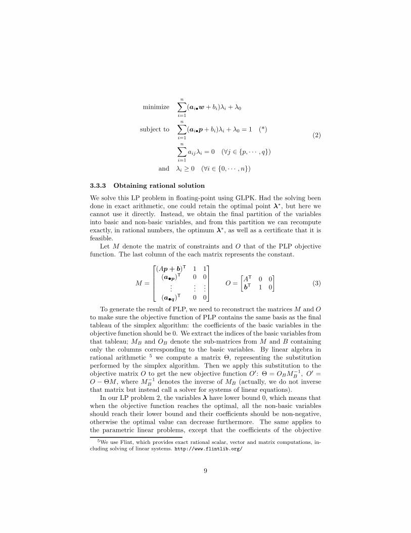
Here is how we process a vector w from the working set. We solve the LPproblem:

8

minimizen∑

i=1

(ai•w + bi)λi + λ0

subject to

n∑

i=1

(ai•p+ bi)λi + λ0 = 1 (*)

n∑

i=1

aijλi = 0 (∀j ∈ {p, · · · , q})

and λi ≥ 0 (∀i ∈ {0, · · · , n})

(2)

3.3.3 Obtaining rational solution

We solve this LP problem in floating-point using GLPK. Had the solving beendone in exact arithmetic, one could retain the optimal point λ∗, but here wecannot use it directly. Instead, we obtain the final partition of the variablesinto basic and non-basic variables, and from this partition we can recomputeexactly, in rational numbers, the optimum λ∗, as well as a certificate that it isfeasible.

Let M denote the matrix of constraints and O that of the PLP objectivefunction. The last column of the each matrix represents the constant.

M =

(Ap+ b)T 1 1(a•p)

T 0 0...

......

(a•q)T 0 0

O =

[AT 0 0bT 1 0

]

(3)

To generate the result of PLP, we need to reconstruct the matrices M and O

to make sure the objective function of PLP contains the same basis as the finaltableau of the simplex algorithm: the coefficients of the basic variables in theobjective function should be 0. We extract the indices of the basic variables fromthat tableau; MB and OB denote the sub-matrices from M and B containingonly the columns corresponding to the basic variables. By linear algebra inrational arithmetic 5 we compute a matrix Θ, representing the substitutionperformed by the simplex algorithm. Then we apply this substitution to theobjective matrix O to get the new objective function O′: Θ = OBM

−1

B , O′ =O − ΘM , where M−1

B denotes the inverse of MB (actually, we do not inversethat matrix but instead call a solver for systems of linear equations).

In our LP problem 2, the variables λ have lower bound 0, which means thatwhen the objective function reaches the optimal, all the non-basic variablesshould reach their lower bound and their coefficients should be non-negative,otherwise the optimal value can decrease furthermore. The same applies tothe parametric linear problems, except that the coefficients of the objective

5We use Flint, which provides exact rational scalar, vector and matrix computations, in-cluding solving of linear systems. http://www.flintlib.org/

9

function may contain parameters; thus the sign conditions on these coefficientsis translated to linear inequalities on these parameters. Each non-zero columnin O′ represents a function in x, which is the coefficient of a non-basic variable.The conjunction of constraints (O′

•j)Tx ≥ 0 constitute the region of x where

j belongs to the indices of non-basic variables. This conjunction of constraintsmay be redundant: we thus call the minimization procedure over it.

4 Checkers and rational solvers

We compared our results with those from NewPolka. We tested about 1.75million polyhedra in our benchmarks. In only 3 cases, round-off errors caused 1face being missed. In this section, we explain how we modified our algorithm towork around this difficulty. The resulting implementation then computes exactlysolutions to parametric linear programs, and thus exactly the same polyhedraas NewPolka.

4.1 Verifying feasibility of the result from GLPK

GLPK uses a threshold (10−7 by default) to check feasibility, that is, if thesolution it proposes truly is a solution. It may report a feasible result whenthe problem is in fact infeasible. Assume that we have an LP problem whoseconstraints are C1 : λ1 ≥ 0, C2 : λ2 ≥ 0, C3 : λ1 + λ2 ≤ 10−8, GLPK will return(0, 0) as a solution, whereas it is not.

We use flint to compute the row echelon form of the rational matrix ofconstraints, so that the pivots are the coefficients of basic variables. We obtain[I A′] = [b] 6, where A′ are the coefficients of the non-basic variables. Whenthe LP problem reaches an optimum, the non-basic variables are at their lowerbound 0, so the value of the basic variables are just the value of b. As we havethe constraints that the variables are non-negative, we thus just need to verifythat all coordinates in b are non-negative. If it is not in this case, it means thatGLPK does not have enough precision, which is likely due to an ill-conditionedsubproblem. In this case, we start a textbook implementation of the simplexalgorithm in rational arithmetic.

GLPK may also report an optimal solution which is in fact not optimized.We did not provide a checker for this situation, as even if the solution is not op-timized in the required region, it is optimized in anther region which is probablyadjacent to the expected one. We keep the obtained solution, and add extratask points between the regions if they are not adjacent. Besides the adjacencychecker guarantees there will be no missed face.

4.2 Flat regions

Our regions are obtained from the rational matrix, and then they are convertedinto floating-point representation. As the regions are normalized and intersect

6There may be rows of all zeros in the bottom of the matrix.

10

at the same point, they are in the shape of cones. During the conversion,the constrains will lose accuracy, and thus a cone could be misjudged as flat,meaning it has empty interior. For instance, we have a cone {C1 : −

100000001

10000000x1+

x2 ≤ 0, C2 : 100000000

10000000x1 − x2 ≤ 0}, which is not flat. After conversion, C1 and

C2 will be represented in floating-point numbers as {C1 : −10.0x1 + x2 ≤ 0, C2 :10.0x1 − x2 ≤ 0}, and the floating-point cone is flat.

In this case we invoke a rational simplex solver to check the region by shiftingall the constraints to the interior direction. If the region becomes infeasibleafter shifting, then the region is really flat; otherwise we launch a rationalminimization algorithm, which is implemented using Farkas Lemma, to obtainthe minimized region.

4.3 Computing an irredundancy witness point

In the minimization algorithm, the checker makes sure that the constraintswhich cannot be determined by floating-point algorithm will be regarded asredundant constraints. In the meantime these constraints are marked as uncer-tainty. If the polyhedron to be minimized is also represented by rational num-bers, a rational solver will be launched to determine the uncertain constraints.As in our PLP algorithm all the regions are represented by both floating-pointand rational numbers, the rational solver can always be executed when thereare uncertain constrains.

Consider the case of computing the irredundant witness point of the con-straint Ci, we need to solve a feasibility problem: Ci : aix < bi and Cj : ajx ≤bj, ∀j 6= i. For efficiency, we solve this problem in floating point. However,GLPK does not support strict inequalities, thus we need tricks to deal withthem.

One method is to shift the inequality constraint a little and obtain a non-strict inequality C′

1 : a1x ≤ b1 − ǫ, where ǫ is a positive constant. This methodis however difficult to apply properly because of the need to find a suitable ǫ.If ǫ is small, we are likely to obtain a point too close to the constraint C1; ifǫ is too large, perhaps we cannot find any point. One exception is that whenthe polyhedron is a cone, we can always find a satisfiable point by shifting theconstraints, no matter how large ǫ is.

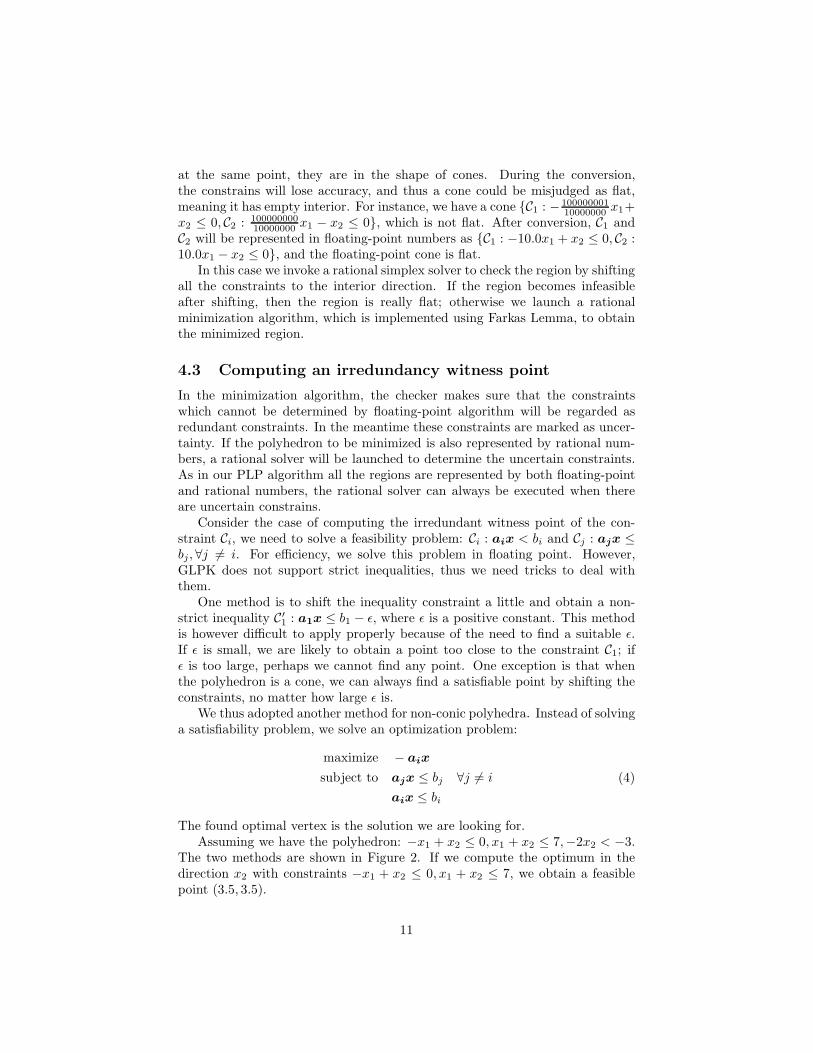
We thus adopted another method for non-conic polyhedra. Instead of solvinga satisfiability problem, we solve an optimization problem:

maximize − aix

subject to ajx ≤ bj ∀j 6= i

aix ≤ bi

(4)

The found optimal vertex is the solution we are looking for.Assuming we have the polyhedron: −x1 + x2 ≤ 0, x1 + x2 ≤ 7,−2x2 < −3.

The two methods are shown in Figure 2. If we compute the optimum in thedirection x2 with constraints −x1 + x2 ≤ 0, x1 + x2 ≤ 7, we obtain a feasiblepoint (3.5, 3.5).

11

1 2 3 4 5 6

1

2

3

4

5

1 2 3 4 5 6

1

2

3

4

5

Figure 2: Solving an optimization problem instead of a feasibility problem.

However the floating-point solver could misjudge, thus the found optimalvertex p could be infeasible. Hence we need to test aip ≤ bi − t, where t is theGLPK threshold. If the test fails, we will use the rational simplex algorithmto compute the Farkas combination: the constraint is really irredundant if thecombination does not exist.

4.4 Adjacency checker

We shall now prove that no face is missed if and only if for each region and eachboundary of this region, another region is found which shares that boundary.

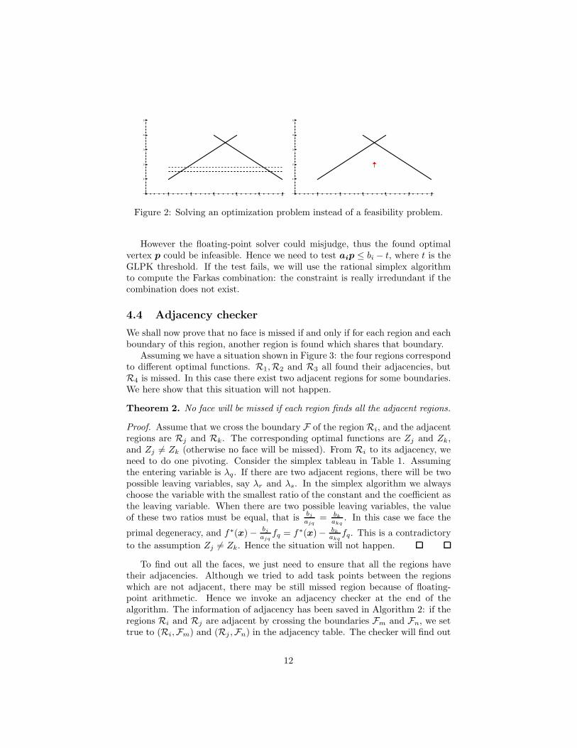
Assuming we have a situation shown in Figure 3: the four regions correspondto different optimal functions. R1,R2 and R3 all found their adjacencies, butR4 is missed. In this case there exist two adjacent regions for some boundaries.We here show that this situation will not happen.

Theorem 2. No face will be missed if each region finds all the adjacent regions.

Proof. Assume that we cross the boundary F of the region Ri, and the adjacentregions are Rj and Rk. The corresponding optimal functions are Zj and Zk,and Zj 6= Zk (otherwise no face will be missed). From Ri to its adjacency, weneed to do one pivoting. Consider the simplex tableau in Table 1. Assumingthe entering variable is λq. If there are two adjacent regions, there will be twopossible leaving variables, say λr and λs. In the simplex algorithm we alwayschoose the variable with the smallest ratio of the constant and the coefficient asthe leaving variable. When there are two possible leaving variables, the valueof these two ratios must be equal, that is

bjajq

= bkakq

. In this case we face the

primal degeneracy, and f∗(x)−bjajq

fq = f∗(x)− bkakq

fq. This is a contradictory

to the assumption Zj 6= Zk. Hence the situation will not happen.

To find out all the faces, we just need to ensure that all the regions havetheir adjacencies. Although we tried to add task points between the regionswhich are not adjacent, there may be still missed region because of floating-point arithmetic. Hence we invoke an adjacency checker at the end of thealgorithm. The information of adjacency has been saved in Algorithm 2: if theregions Ri and Rj are adjacent by crossing the boundaries Fm and Fn, we settrue to (Ri,Fm) and (Rj ,Fn) in the adjacency table. The checker will find out

12

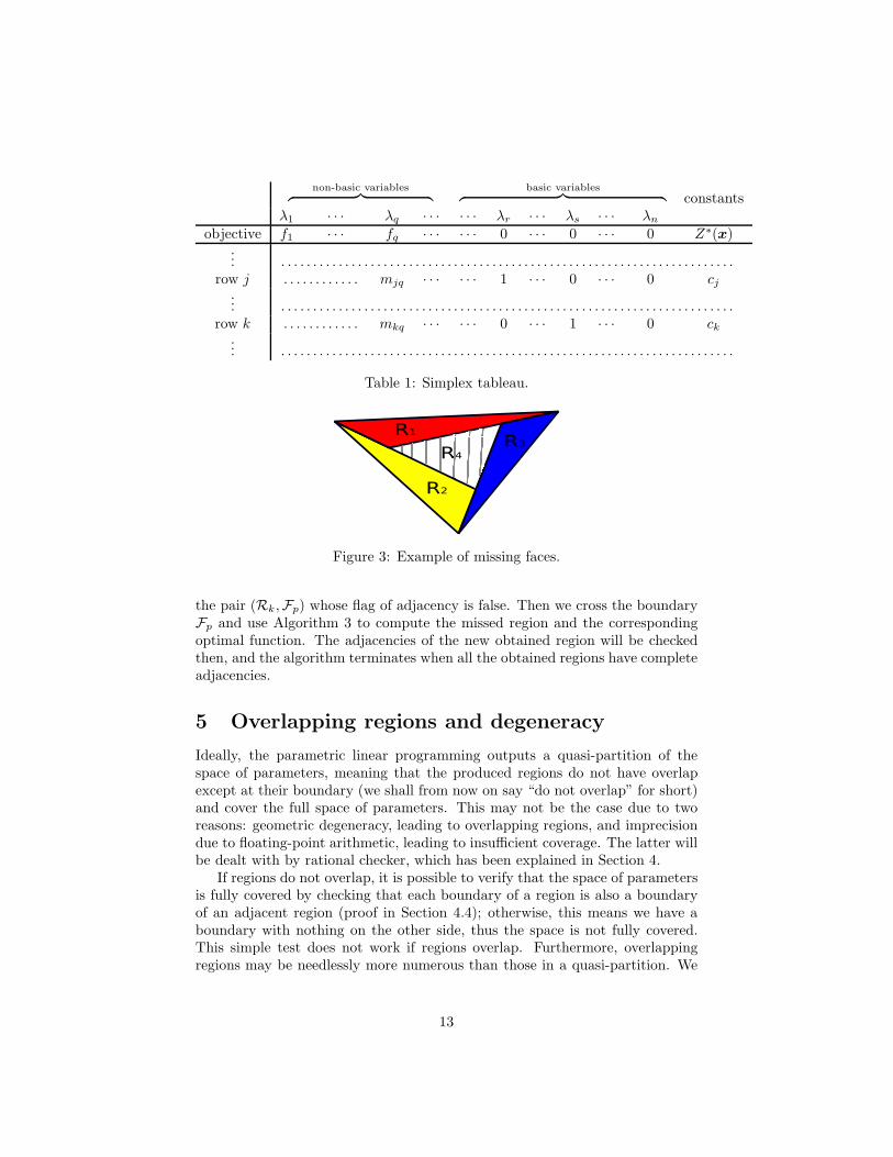
non-basic variables︷ ︸︸ ︷

basic variables︷ ︸︸ ︷ constants

λ1 · · · λq · · · · · · λr · · · λs · · · λn

objective f1 · · · fq · · · · · · 0 · · · 0 · · · 0 Z∗(x)... . . . . . . . . . . . . . . . . . . . . . . . . . . . . . . . . . . . . . . . . . . . . . . . . . . . . . . . . . . . . . . . . . . . . . . .

row j . . . . . . . . . . . . mjq · · · · · · 1 · · · 0 · · · 0 cj... . . . . . . . . . . . . . . . . . . . . . . . . . . . . . . . . . . . . . . . . . . . . . . . . . . . . . . . . . . . . . . . . . . . . . . .

row k . . . . . . . . . . . . mkq · · · · · · 0 · · · 1 · · · 0 ck... . . . . . . . . . . . . . . . . . . . . . . . . . . . . . . . . . . . . . . . . . . . . . . . . . . . . . . . . . . . . . . . . . . . . . . .

Table 1: Simplex tableau.

R1

R2

R3

R4

Figure 3: Example of missing faces.

the pair (Rk,Fp) whose flag of adjacency is false. Then we cross the boundaryFp and use Algorithm 3 to compute the missed region and the correspondingoptimal function. The adjacencies of the new obtained region will be checkedthen, and the algorithm terminates when all the obtained regions have completeadjacencies.

5 Overlapping regions and degeneracy

Ideally, the parametric linear programming outputs a quasi-partition of thespace of parameters, meaning that the produced regions do not have overlapexcept at their boundary (we shall from now on say “do not overlap” for short)and cover the full space of parameters. This may not be the case due to tworeasons: geometric degeneracy, leading to overlapping regions, and imprecisiondue to floating-point arithmetic, leading to insufficient coverage. The latter willbe dealt with by rational checker, which has been explained in Section 4.

If regions do not overlap, it is possible to verify that the space of parametersis fully covered by checking that each boundary of a region is also a boundaryof an adjacent region (proof in Section 4.4); otherwise, this means we have aboundary with nothing on the other side, thus the space is not fully covered.This simple test does not work if regions overlap. Furthermore, overlappingregions may be needlessly more numerous than those in a quasi-partition. We

13

thus have two reasons to modify our algorithm to get rid of overlapping regions.Let us see how overlapping regions occur. In a non-degenerate parametric

linear program, for a given optimization function, there is only one optimalvertex (no dual degeneracy), and this optimal vertex is described by only oneoptimal basis (no primal degeneracy), i.e., there is a single optimal partitionof variables into basic and non-basic. Thus, in a non-degenerate parametriclinear program, for a given vector of parameters there is one single optimalbasis (except at boundaries), meaning that each optimal function correspondsto one region. However when there is degeneracy, there will be multiple basescorresponding to one optimal function, and each of them computes a region.These regions may be overlapping. We call the regions corresponds to the sameoptimal function degeneracy regions.

Theorem 3. There will be no overlapping regions if there is no degeneracy.

Proof. In parametric linear programming, the regions are yielded by the parti-tion of variables into basic and non-basic, i.e., each region corresponds to onebasis. The parameters within one region lead the PLP problem to the samepartition of variables. If there are overlapping regions, say Ri and Rj , the PLPproblem will be optimized by multiple bases when the parameters belong toRi ∩Rj . In this case there must be degeneracy: these multiple bases may leadto multiple optimal vertex when we have dual degeneracy, or the same optimalvertex when we have primal degeneracy. By transposition, we know that if thereis no degeneracy the PLP problem will always obtain a unique basis with givenparameters, and there will be no overlapping regions.

We thus need to get rid of degeneracy. We shall first prove that thereis no dual degeneracy in our PLP algorithm, and then deal with the primaldegeneracy.

5.1 Dual degeneracy

Theorem 4. For projection and convex hull, the parametric linear programexhibits no dual degeneracy.

Proof. We shall see that the normalization constraint (the constraint (∗) inProblem 1) present in the parametric linear programs defining projection andconvex hull prevents dual degeneracy.

Assume that at the optimum Z∗(x) we have the simplex tableau in Table1. λk denote the decision variables: λk ≥ 0. In the current dictionary, theparametric coefficients of the objective function is fk = a′

i•x + b′i. Assumingthe variable leaving the basis is λr, and the entering variable is λq. Then λr isdefined by the jth row as

∑

j mjpλp +λr = cj , where λp are nonbasic variables.That means λr = cj when the nonbasic variables reach their lower bound, whichis 0 here.

Now we look for another optimum by doing one pivoting. As the currentdictionary is feasible, we must have cj ≥ 0. To maintain the feasibility, we must

14

choose λq such that mjq > 0. As we only choose the non-basic variable whosecoefficient is negative to enter the basis, then we know fq < 0. By pivoting weobtain the new objective function Z ′(λ,x) = Z(λ,x)−fq

cjmjq

. The new optimal

function is:Z∗

′

(x) = Z∗(x)− fqcj

mjq

(5)

Let us assume that a dual degeneracy occurs, which means that we obtainthe same objective function after the pivoting, i.e., Z∗

′

(x) = tZ∗(x), wheret is a positive constant. Due to the normalization constraint at the point x0

enforcing Z∗′

(x0) = Z∗(x0) = 1, we have t = 1. Hence we will obtain

Z∗′

(x) = Z∗(x) (6)

Considering the equation 5 and 6 we obtain

fqcj

mjq

= 0 (7)

Since fq 6= 0, cj must equal to 0, which means that we in fact faced a primaldegeneracy.

Let D1 = fqcjmjq

, where the subscript of D1 denotes the first pivoting. As

cj ≥ 0, fq < 0 and mjq > 0, we know D1 ≤ 0. Similarly in each pivoting wehave Di ≤ 0.

If we generalize the situation above to N rounds of pivoting, we will obtain:

Z∗′

(x) = Z∗(x)−

N∑

i=1

Di (8)

If there is dual degeneracy Z∗′

(x) = Z∗(x), and then

N∑

i=1

Di = 0 (9)

As ∀i,Di ≤ 0, Equation 9 implies ∀i,Di = 0, which is possible if and only if allthe cj equal to 0. For the same reason as above, in this case we can only haveprimal degeneracy.

5.2 Primal degeneracy

Many methods to deal with primal degeneracy in non-parametric linear pro-gramming are known [3, 10, 8]; fewer in parametric linear programming [13].We implemented an approach to avoid overlapping regions based on the workof Jones et al. [13], which used the perturbation method [10]. The algorithm isshown in Algorithm 3. Once entering a new region, we check if there is primaldegeneracy: it occurs when one or several basic variables equal zero. In this casewe will explore all degeneracy regions for the same optimum, using, as explainedbelow, a method avoiding overlaps.

15

Let us consider a projected polyhedra in 3 dimensions with primal degener-acy, because of which there are multiple regions corresponding to the same face.Figure 4 shows the 2D view of the face. The yellow and red triangles representthe intersection of the regions with their face. Figure 4a shows the disappointcase where the regions are overlapping. The reason is that when the parame-ters locate in the orange part, two different bases will lead the constructed LPproblem to optimum. We aim to avoid the overlap and obtain the result eitherin Figure 4b or in Figure 4c.

(a) (b) (c)

Figure 4: Example of overlapping regions.

Our solution against overlaps is to make the optimal basis unique for givenparameters of the objective function by adding perturbation terms to the rightside of the constraints [13]. These perturbation terms are “infinitesimal”, mean-ing that the right-hand side, instead of being a vector of rational scalars, be-comes a matrix where the first column corresponds to the original vector, thesecond column corresponds to the first infinitesimal, the third column to thesecond infinitesimal, etc. The same applies to λ. Instead of comparing scalarcoordinates using the usual ordering on rational numbers, we compare line vec-tors of rationals with the lexicographic ordering. After the perturbation, therewill be no primal degeneracy as all the right-hand side of the constraints cannotbe equal.

The initial perturbation matrix is a k ∗ k identity matrix: Mp = I, wherek is the number of constraints. Then the perturbation matrix will be updatedas the reconstruction of the constraint matrix. After adding this perturbationmatrix, the right-hand side becomes B = [b|Mp]. The new constants are vectorsin the form of vi = [bi 0 · · · 1 · · · 0]. We compare the vectors by lexico-order:vi > vj if the first non-zero element of vi is larger than that of vj .

To obtain a new basis, in contrast to working with non-degeneracy regions,we do not solve the problem using floating point solver. Instead, we pivotdirectly on the perturbed rational matrix. Each non-basic variable will be chosenas entering variable. Then from all the constraints in which bi = 0, we selectthe basic variable λl in Ci whose ratio vi

aijis smallest as the leaving variable,

where j is the index of the entering variable. If such a leaving variable exist, wewill obtain a degeneracy region: as bi = 0, the new optimal function will remainthe same. Otherwise it means that a new optimal function will be obtained

16

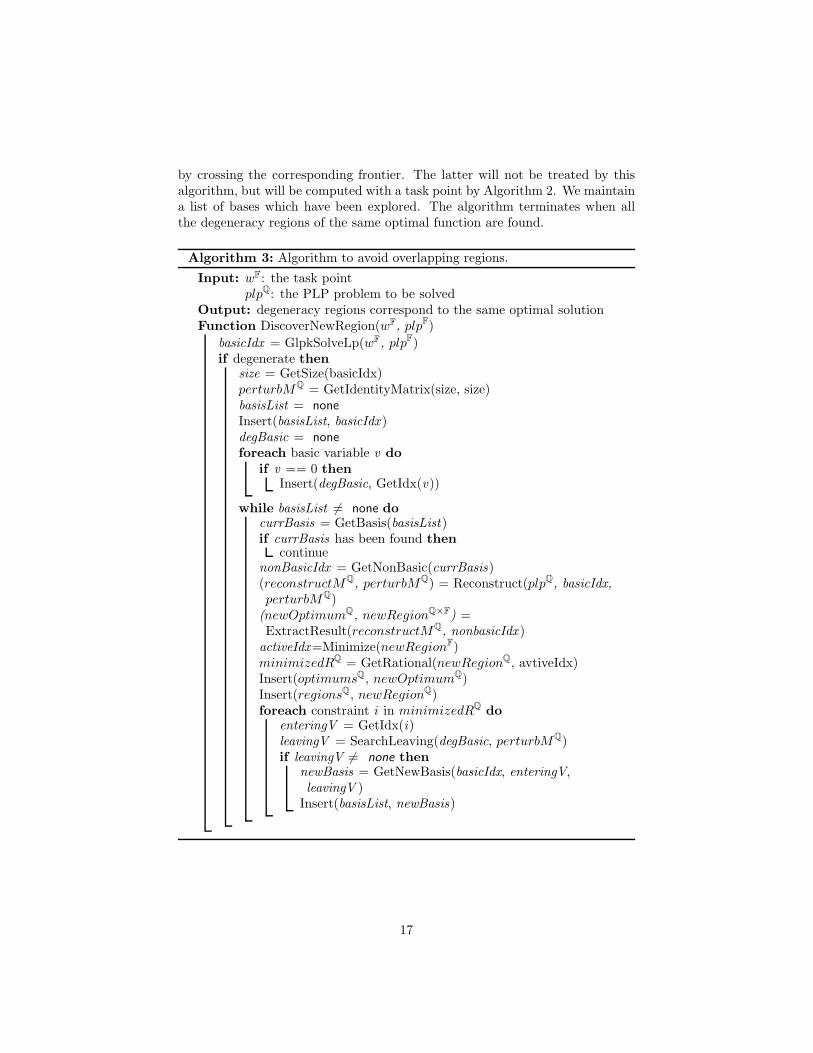
by crossing the corresponding frontier. The latter will not be treated by thisalgorithm, but will be computed with a task point by Algorithm 2. We maintaina list of bases which have been explored. The algorithm terminates when allthe degeneracy regions of the same optimal function are found.

Algorithm 3: Algorithm to avoid overlapping regions.

Input: wF: the task pointplpQ: the PLP problem to be solved

Output: degeneracy regions correspond to the same optimal solutionFunction DiscoverNewRegion(wF, plpF)

basicIdx = GlpkSolveLp(wF, plpF)if degenerate then

size = GetSize(basicIdx)perturbMQ = GetIdentityMatrix(size, size)basisList = none

Insert(basisList, basicIdx )degBasic = none

foreach basic variable v do

if v == 0 thenInsert(degBasic, GetIdx(v))

while basisList 6= none docurrBasis = GetBasis(basisList)if currBasis has been found then

continuenonBasicIdx = GetNonBasic(currBasis)(reconstructMQ, perturbMQ) = Reconstruct(plpQ, basicIdx,perturbMQ)(newOptimumQ, newRegionQ×F) =ExtractResult(reconstructMQ, nonbasicIdx )activeIdx=Minimize(newRegionF)minimizedRQ = GetRational(newRegionQ, avtiveIdx)Insert(optimumsQ, newOptimumQ)Insert(regionsQ, newRegionQ)foreach constraint i in minimizedRQ

doenteringV = GetIdx(i)leavingV = SearchLeaving(degBasic, perturbMQ)if leavingV 6= none then

newBasis = GetNewBasis(basicIdx, enteringV,leavingV )Insert(basisList, newBasis)

17

6 Experiments

In this section, we analyze the performance of our parametric linear program-ming solver on projection operations. We compare its performance with that ofthe NewPolka library of Apron7 and ELINA library [21]. Since NewPolka andELINA do not exploit parallelism, we compare it to our library running withonly one thread.

We used three libraries in our implementation:

• Eigen 3.3.2 for floating-point vector and matrix operations;

• FLINT 2.5.2 for rational arithmetic, vector and matrix operations;

• GLPK 4.6.4 for solving linear programs in floating-point.

The experiments are carried out on 2.30GHz Intel Core i5-6200U CPU.

6.1 Experiments on random polyhedra

6.1.1 Benchmarks

The benchmark contains randomly-generated polyhedra, in which the coeffi-cients of constraints are in the range of -50 to 50. Each polyhedron has 4parameters: number of constraints (CN), number of variables (VN), projectionratio(PR) and density (D). The projection ratio is the proportion of eliminatedvariables: for example if we eliminate 6 variables out of 10, the projection ratiois 60%. Density represents the ratio of zero coefficients: if there are 2 zeros in10 coefficients, density is 20%. In each experiment, we project 10 polyhedragenerated with the same parameters. To smooth out experimental noise, we doeach experiment 5 times, i.e., 50 executions for each set of parameters. Thenwe calculate the average execution time of the 50 executions.

6.1.2 Experimental results

We illustrate the execution time (in seconds) by line charts. The blue line is theperformance of NewPolka library of Apron, and the red line is that of our serialPLP algorithm. To illustrate the performance benefits from the floating-pointarithmetic, we turned off GLPK and always use the rational LP solver, andthe execution time is shown by the orange lines8. It is shown that solving theLP problems in floating-point numbers and reconstructing the rational simplextableau leads to significant improvement of performance.

By a mount of experiments, we found that when the parameters CN =19, V N = 8, PR = 62.5% and D = 37.5%, the execution time of PLP andApron are similar, so we maintain three of them and vary the other to analyzethe variation of performance.

7https://github.com/antoinemine/apron8The minimization is still computed in floating-point numbers.

18

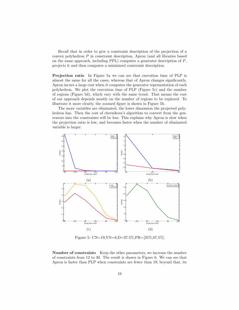
Recall that in order to give a constraint description of the projection of aconvex polyhedron P in constraint description, Apron (and all libraries basedon the same approach, including PPL) computes a generator description of P ,projects it and then computes a minimized constraint description.

Projection ratio In Figure 5a we can see that execution time of PLP isalmost the same for all the cases, whereas that of Apron changes significantly.Apron incurs a large cost when it computes the generator representation of eachpolyhedron. We plot the execution time of PLP (Figure 5c) and the numberof regions (Figure 5d), which vary with the same trend. That means the costof our approach depends mostly on the number of regions to be explored. Toillustrate it more clearly, the zoomed figure is shown in Figure 5b.

The more variables are eliminated, the lower dimension the projected poly-hedron has. Then the cost of chernikova’s algorithm to convert from the gen-erators into the constraints will be less. This explains why Apron is slow whenthe projection ratio is low, and becomes faster when the number of eliminatedvariable is larger.

25% 37.5% 50% 62.5% 75% 87.5%

projection ratio

0

50

100

150

200

250

300

350

time(s)

plpapron

(a)

50% 62.5% 75%

projection ratio

0.2

0.4

0.6

0.8

1

1.2

1.4

1.6

time(s)

apronplp

(b)

25% 37.5% 50% 62.5% 75% 87.5%

projection ratio

0

0.1

0.2

0.3

0.4

0.5

time(s)

plprational

(c)

25% 37.5% 50% 62.5% 75% 87.5%

projection ratio

0

50

100

150

200

250

number

region number

(d)

Figure 5: CN=19,VN=8,D=37.5%,PR=[25%,87.5%]

Number of constraints Keep the other parameters, we increase the numberof constraints from 12 to 30. The result is shown in Figure 6. We can see thatApron is faster than PLP when constraints are fewer than 19; beyond that, its

19

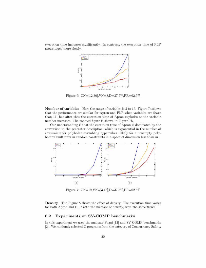
execution time increases significantly. In contrast, the execution time of PLPgrows much more slowly.

15 20 25 30

constraint number

0

0.5

1

1.5

2

2.5

time(s)

apronplprational

Figure 6: CN=[12,30],VN=8,D=37.5%,PR=62.5%

Number of variables Here the range of variables is 3 to 15. Figure 7a showsthat the performance are similar for Apron and PLP when variables are fewerthan 11, but after that the execution time of Apron explodes as the variablenumber increases. The zoomed figure is shown in Figure 7b.

Our understanding is that the execution time of Apron is dominated by theconversion to the generator description, which is exponential in the number ofconstraints for polyhedra resembling hypercubes—likely for a nonempty poly-hedron built from m random constraints in a space of dimension less than m.

3 5 7 9 11 13 15

variable number

0

50

100

150

time(s)

plpapron

(a)

3 5 7 9 11 13 15

variable number

0

0.5

1

1.5

2

2.5

3

time(s)

plpapronrational

(b)

Figure 7: CN=19,VN=[3,15],D=37.5%,PR=62.5%

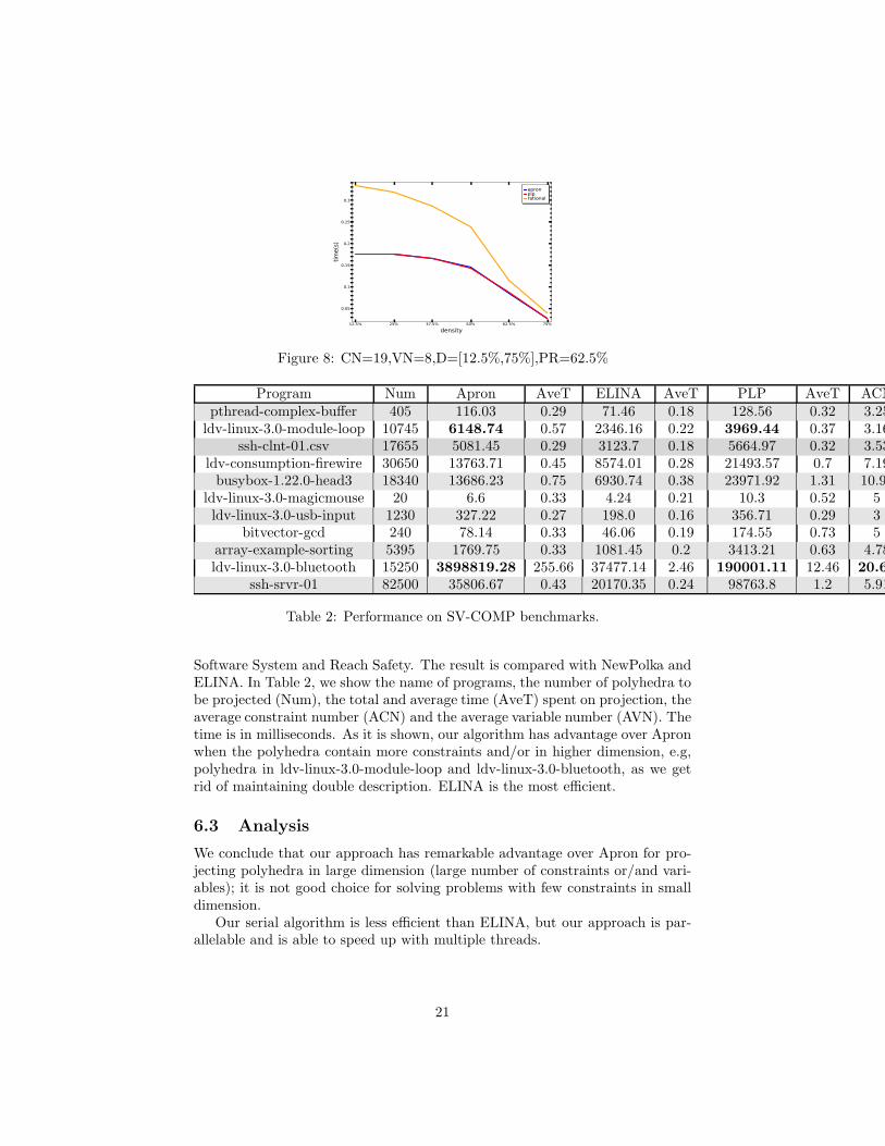
Density The Figure 8 shows the effect of density. The execution time variesfor both Apron and PLP with the increase of density, with the same trend.

6.2 Experiments on SV-COMP benchmarks

In this experiment we used the analyzer Pagai [12] and SV-COMP benchmarks[2]. We randomly selected C programs from the category of Concurrency Safety,

20

12.5% 25% 37.5% 50% 62.5% 75%

density

0.05

0.1

0.15

0.2

0.25

0.3

time(s)

apronplprational

Figure 8: CN=19,VN=8,D=[12.5%,75%],PR=62.5%

Program Num Apron AveT ELINA AveT PLP AveT ACNpthread-complex-buffer 405 116.03 0.29 71.46 0.18 128.56 0.32 3.25

ldv-linux-3.0-module-loop 10745 6148.74 0.57 2346.16 0.22 3969.44 0.37 3.16ssh-clnt-01.csv 17655 5081.45 0.29 3123.7 0.18 5664.97 0.32 3.53

ldv-consumption-firewire 30650 13763.71 0.45 8574.01 0.28 21493.57 0.7 7.19busybox-1.22.0-head3 18340 13686.23 0.75 6930.74 0.38 23971.92 1.31 10.94

ldv-linux-3.0-magicmouse 20 6.6 0.33 4.24 0.21 10.3 0.52 5ldv-linux-3.0-usb-input 1230 327.22 0.27 198.0 0.16 356.71 0.29 3

bitvector-gcd 240 78.14 0.33 46.06 0.19 174.55 0.73 5array-example-sorting 5395 1769.75 0.33 1081.45 0.2 3413.21 0.63 4.78ldv-linux-3.0-bluetooth 15250 3898819.28 255.66 37477.14 2.46 190001.11 12.46 20.62

ssh-srvr-01 82500 35806.67 0.43 20170.35 0.24 98763.8 1.2 5.91

Table 2: Performance on SV-COMP benchmarks.

Software System and Reach Safety. The result is compared with NewPolka andELINA. In Table 2, we show the name of programs, the number of polyhedra tobe projected (Num), the total and average time (AveT) spent on projection, theaverage constraint number (ACN) and the average variable number (AVN). Thetime is in milliseconds. As it is shown, our algorithm has advantage over Apronwhen the polyhedra contain more constraints and/or in higher dimension, e.g,polyhedra in ldv-linux-3.0-module-loop and ldv-linux-3.0-bluetooth, as we getrid of maintaining double description. ELINA is the most efficient.

6.3 Analysis

We conclude that our approach has remarkable advantage over Apron for pro-jecting polyhedra in large dimension (large number of constraints or/and vari-ables); it is not good choice for solving problems with few constraints in smalldimension.

Our serial algorithm is less efficient than ELINA, but our approach is par-allelable and is able to speed up with multiple threads.

21

7 Conclusion and future work

We have presented an algorithm to project convex polyhedra via parametriclinear programming. It internally uses floating-point numbers, and then theexact result is constructed over the rationals. Due to floating-point round-offerrors, some faces may be missed by the main pass of our algorithm. However,we can detect this situation and recover the missing faces using an exact solver.

We currently store the regions that have been explored into an unstructuredarray; checking whether an optimization direction is covered by an existingregion is done by linear search. This could be improved in two ways: i) regionscorresponding to the same optimum (primal degeneracy) could be merged intoa single region; ii) regions could be stored in a structure allowing fast search.For instance, we could use a binary tree where each node is labeled with ahyperplane, and each path from the root corresponds to a conjunction of half-spaces; then each region is stored only in the paths such that the associatedhalf-spaces intersects the region.

References

[1] Roberto Bagnara, Patricia M Hill, and Enea Zaffanella. “The Parma Poly-hedra Library: Toward a complete set of numerical abstractions for theanalysis and verification of hardware and software systems”. In: Scienceof Computer Programming 72.1 (2008), pp. 3–21.

[2] Dirk Beyer. “Automatic verification of C and Java programs: SV-COMP2019”. In: International Conference on Tools and Algorithms for the Con-struction and Analysis of Systems. Springer. 2019, pp. 133–155.

[3] Robert G Bland. “New finite pivoting rules for the simplex method”. In:Mathematics of operations Research 2.2 (1977), pp. 103–107.

[4] NV Chernikova. “Algorithm for discovering the set of all the solutions ofa linear programming problem”. In: USSR Computational Mathematicsand Mathematical Physics 8.6 (1968), pp. 282–293.

[5] Camille Coti, David Monniaux, and Hang Yu. “Parallel parametric lin-ear programming solving, and application to polyhedral computations”.In: International Conference on Computational Science. Springer. 2019,pp. 566–572.

[6] Patrick Cousot and Radhia Cousot. “Abstract interpretation: a unifiedlattice model for static analysis of programs by construction or approxi-mation of fixpoints”. In: Proceedings of the 4th ACM SIGACT-SIGPLANsymposium on Principles of programming languages. ACM. 1977, pp. 238–252.

[7] Patrick Cousot and Nicolas Halbwachs. “Automatic discovery of linearrestraints among variables of a program”. In: Proceedings of the 5th ACMSIGACT-SIGPLAN symposium on Principles of programming languages.ACM. 1978, pp. 84–96.

22

[8] George B Dantzig. “Application of the simplex method to a transportationproblem”. In: Activity Analysis and Production and Allocation (1951).

[9] George B Dantzig. Fourier-Motzkin elimination and its dual. Tech. rep.STANFORD UNIV CA DEPT OF OPERATIONS RESEARCH, 1972.

[10] George B Dantzig and Mukund N Thapa. Linear programming 2: theoryand extensions. Springer Science & Business Media, 2006.

[11] Alexis Fouilhe. “Revisiting the abstract domain of polyhedra: constraints-only representation and formal proof”. PhD thesis. Universite GrenobleAlpes, 2015.

[12] Julien Henry, David Monniaux, and Matthieu Moy. “Pagai: A path sensi-tive static analyser”. In: Electronic Notes in Theoretical Computer Science289 (2012), pp. 15–25.

[13] Colin N Jones, Eric C Kerrigan, and Jan M Maciejowski. “Lexicographicperturbation for multiparametric linear programming with applications tocontrol”. In: Automatica 43.10 (2007), pp. 1808–1816.

[14] Colin N Jones, Eric C Kerrigan, and Jan M Maciejowski. “On polyhe-dral projection and parametric programming”. In: Journal of Optimiza-tion Theory and Applications 138.2 (2008), pp. 207–220.

[15] Tim King, Clark Barrett, and Cesare Tinelli. “Leveraging linear and mixedinteger programming for SMT”. In: Proceedings of the 14th Conference onFormal Methods in Computer-Aided Design. FMCAD Inc. 2014, pp. 139–146.

[16] Herv Le Verge. A note on Chernikova’s Algorithm. Tech. rep. 635. IRISA,1992. url: https://www.irisa.fr/polylib/document/cher.ps.gz.

[17] Alexandre Marechal. “New Algorithmics for Polyhedral Calculus via Para-metric Linear Programming”. Theses. UGA - Universite Grenoble Alpes,Dec. 2017. url: https://hal.archives-ouvertes.fr/tel-01695086.

[18] Alexandre Marechal, David Monniaux, and Michael Perin. “Scalable minimizing-operators on polyhedra via parametric linear programming”. In: Interna-tional Static Analysis Symposium. Springer. 2017, pp. 212–231.

[19] Alexandre Marechal and Michael Perin. “Efficient elimination of redun-dancies in polyhedra by raytracing”. In: International Conference on Ver-ification, Model Checking, and Abstract Interpretation. Springer. 2017,pp. 367–385.

[20] David Monniaux. “On using floating-point computations to help an ex-act linear arithmetic decision procedure”. In: International Conference onComputer Aided Verification. Springer. 2009, pp. 570–583.

[21] Gagandeep Singh, Markus Puschel, and Martin Vechev. “Fast polyhedraabstract domain”. In: ACM SIGPLAN Notices. Vol. 52. 1. ACM. 2017,pp. 46–59.

23