An efficient streaming algorithm for spectral proper

Please cite this article as: O.T. Schmidt and A. Towne, An efficient streaming algorithm for spectral proper orthogonal decomposition, Computer Physics Communications(2018), https://doi.org/10.1016/j.cpc.2018.11.009.

Computer Physics Communications xxx (xxxx) xxx

Contents lists available at ScienceDirect

Computer Physics Communications

journal homepage: www.elsevier.com/locate/cpc

An efficient streaming algorithm for spectral proper orthogonaldecompositionOliver T. Schmidt a,⇤, Aaron Towne b

aUniversity of California San Diego, La Jolla, CA 92093, USA

bUniversity of Michigan, Ann Arbor, MI 48109, USA

a r t i c l e i n f o

Article history:

Received 17 November 2017Received in revised form 12November 2018Accepted 14 November 2018Available online xxxx

Keywords:

Proper orthogonal decompositionPrincipal component analysisSpectral analysis

a b s t r a c t

A streaming algorithm to compute the spectral proper orthogonal decomposition (SPOD) of stationaryrandom processes is presented. As new data becomes available, an incremental update of the truncatedeigenbasis of the estimated cross-spectral density (CSD) matrix is performed. The algorithm requiresaccess to only one temporal snapshot of the data at a time and converges orthogonal sets of SPOD modesat discrete frequencies that are optimally ranked in terms of energy. We define measures of error andconvergence, and demonstrate the algorithm’s performance on two datasets. The first example considersa high-fidelity numerical simulation of a turbulent jet, and the second example uses optical flow dataobtained from high-speed camera recordings of a stepped spillway experiment. For both cases, the mostenergetic SPOD modes are reliably converged. The algorithm’s low memory requirement enables real-time deployment and allows for the convergence of second-order statistics from arbitrarily long streamsof data. A MATLAB implementation of the algorithm along with a test database for the jet example, canbe found in the Supplementary material.

© 2018 Elsevier B.V. All rights reserved.

1. Introduction

The ability to represent complex dynamics by a small numberof dynamically important modes enables the analysis, modelingand control of high-dimensional systems. Turbulent flows are aprominent example of such systems [1,2]. Proper orthogonal de-composition (POD), also known as principle component analysis(PCA) or Karhunen–Loève decomposition, is a popular modal de-composition technique to extract coherent structures from exper-imental and numerical data. In its most common form [3], POD isconducted in the time domain. It is computed from a time seriesof snapshots and expands the flow field into a sum of productsof spatially orthogonal modes and coefficients with random timedependence. POD modes are optimally ranked in terms of theirvariance, or energy. These properties make PODmodes well suitedfor low-order models based on Galerkin projection of the Navier–Stokes equations [4,5].

Besides its definitions in the temporal and spatial domains, PODcan also be formulated in the frequency domain. This variant ofPOD called spectral proper orthogonal decomposition (SPOD), datesback to the early work of Lumley [6] and takes advantage oftemporal homogeneity. This makes it ideally suited for statisti-cally (wide-sense) stationary data [7]. SPOD provides orthogonal

⇤ Corresponding author.E-mail address: [email protected] (O.T. Schmidt).

modes at discrete frequencies that are optimally ranked in termsof energy, and that evolve coherently in both space and time.Perhaps predictably, this optimal space–time representation ofthe data comes at a cost—very long time series are necessary inorder to converge the second-order space–time statistics. This datademand also becomes apparent when comparing SPOD to othermodal decomposition techniques, for example the popular dy-namic mode decomposition (DMD) [8]. For stationary data, SPODmodes correspond to optimally averaged DMD modes computedfrom an ensemble of stochastic realizations of a process [7], forexamplemultiple repetitions of the same experiment. In Section 5,we use two databases consisting of 10,000 and 19,782 snapshots,respectively. Evidently, the SPOD problem quickly becomes com-putationally unmanageable for data with large spatial dimensions.

In this paper, we address this issue by proposing a low-storagestreaming SPOD algorithm that incrementally updates the SPOD asnew data becomes available. Similar algorithms are often referredto as incremental, learning, updating, on-the-fly or online algorithmsin the literature. Streaming algorithms for DMD have been devel-oped recently [9,10], for example. The proposed streaming SPODalgorithm utilizes incremental updates of the singular value de-composition (SVD) of the cross-spectral density (CSD)matrix of thedata. SVDupdating has been an active research topic for almost halfa century, see e.g. [11,12]. In this work, we build on Brand’s [13]incremental singular value decomposition (SVD) by specializingthe method to updates of the estimated CSD matrix. Originallydeveloped for computer vision and audio feature extraction [14],

https://doi.org/10.1016/j.cpc.2018.11.0090010-4655/© 2018 Elsevier B.V. All rights reserved.


2 O.T. Schmidt and A. Towne / Computer Physics Communications xxx (xxxx) xxx

the algorithm has been employed for recommender systems [15],semantics [16], design optimization [17], and a wide spectrum ofother machine learning and data mining applications.

The paper is organized as follows. We first introduce standardor batch SPOD in Section 2 before deriving the streaming algorithmin Section 3. Measures of error and convergence are defined inSection 4. In Section 5, we demonstrate streaming SPOD on twodatasets: a high-fidelity large eddy simulation (LES) of a turbulentjet and experimental optical flow from high-speed camera data ofa stepped spillway. The effect of eigenbasis truncation is addressedin Section 6. In Section 7, we conclude with a discussion of thealgorithm’s computational efficiency and utility in real-time andbig data settings.

2. Batch SPOD

SPOD is the frequency-domain counterpart of standard time-domain or spatial POD. SPOD yields time-harmonic modes thatrepresent structures that evolve coherently in both time andspace [7]. The method is based on an eigendecomposition of theCSD, which in turn is estimated from an ensemble of realizationsof the temporal discrete Fourier transform (DFT) in practice. TheCSD can be estimated using standard spectral estimation tech-niques such as Welch’s method [see e.g. 18] from an ensembleof snapshots. The SPOD formalism is derived from a space–timePODproblemunder the assumption ofwide-sense stationarity. Thereader is referred to [7] for the derivation of the method and anassessment of its properties. In particular, the method’s relationsto DMD and the resolvent operator are interesting from amodelingperspective, as they link SPOD to concepts fromdynamical systemsand hydrodynamics stability theory.

Fig. 1 serves as a visual guide through the batch algorithm.We start with an ensemble of nt snapshots qi = q(ti) 2 Rn

of a wide-sense stationary process q(t) sampled at discrete timest1, t2, . . . , tnt 2 R. By q we denote the state vector. Its total lengthn is equal to the number of grid points nx times the number ofvariables nvar. The temporal mean corresponds to the ensembleaverage defined as

q =1nt

ntX

i=1

qi 2 Rn. (1)

We collect the mean-subtracted snapshots in a data matrix

Q = [q1 � q, q2 � q, . . . , qnt� q] 2 Rn⇥nt (2)

of rank d min{n, nt � 1}. With the goal of estimating the CSD,we apply Welch’s method to the data by segmenting Q into nblkoverlapping blocks

Q(l)

= [q(l)1 � q, q

(l)2 � q, . . . , q(l)

nfreq� q] 2 Rn⇥nfreq (3)

containing nfreq snapshots each. If novlp is the number of snapshotsby which the blocks overlap, then the jth column of the lth blockQ

(l) is given as

q(l)j

= qj+(l�1)(nfreq�novlp) � q. (4)

We assume that each block can be regarded as a statisticallyindependent realization under the ergodicity hypothesis. The pur-pose of the segmentation step is to artificially increase the numberof ensemble members, i.e. Fourier realizations. This method isuseful in the common scenario where a single long dataset withequally sampled snapshots is available, for example from a numer-ical simulation. In situations where the data presents itself in formof independent realizations from the beginning, segmenting neednot be applied. This is the case, for example, if an experiment is

repeated multiple times. Next, the temporal (row-wise) discreteFourier transform

Q(l)

= [q(l)1 , q

(l)2 , . . . , q(l)

nfreq] 2 Rn⇥nfreq (5)

of each block is calculated. A windowing function can be used tomitigate spectral leakage. All realizations of the Fourier transformat the kth frequency are subsequently collected into a new datamatrix

Qk = [q(1)k

, q(2)k

, . . . , q(nblk)k

] 2 Rn⇥nblk . (6)

At this point, we introduce the weighted data matrix

Xk =1pnblk

W12 Qk = [x

(1)k

, x(2)k

, . . . , x(nblk)k

] 2 Rn⇥nblk , (7)

where W 2 Rn⇥n is a positive-definite Hermitian matrix thataccounts for quadrature and possibly other weights associatedwith the discretized inner product

ha, biE = a⇤Wb. (8)

The inner product (8) induces the spatial energy norm k · kE =ph·, ·iE by which we wish to rank the SPOD modes. The product

Sk = XkX⇤

k2 Rn⇥n (9)

defines the weighted CSD matrix of the kth frequency. A factorof 1

nblkseen in other definitions of the CSD is absorbed into our

definition of the weighted data matrix in Eq. (7).SPOD is based on the eigenvalue decomposition

Sk = Uk⇤kU⇤

k(10)

of theCSDmatrix,where⇤k = diag(�k1 , �k2 . . . , �knblk) 2 Rnblk⇥nblk

is the matrix of ranked (in descending order) eigenvalues andUk = [uk1 ,uk2 , . . . ,uknblk

] 2 Rn⇥nblk the corresponding matrix ofeigenvectors. Equivalently, we may consider the economy SVD ofthe weighted data matrix

Xk = Uk⌃ kV⇤

k, (11)

where ⌃ k = diag(�k1 , �k2 . . . , �knblk) 2 Rnblk⇥nblk is the matrix

of singular values and Vk = [vk1 , vk2 , . . . , vknblk ] 2 Rn⇥nblk theright singular vector matrix. This can be shown by rewriting theCSD in terms of the SVD of the data matrix as Sk = XkX

⇤

k=

Uk⌃ kV⇤

kVk⌃ kU

⇤

k= Uk⇤kU

⇤

k. Throughout this paper, we assume

that all Fourier realizations of the flow are linearly independent. Inthe final step, the SPOD modes � and modal energies � 2 are foundas

�k = W�

12 Uk = [�

k1, �

k2, . . . ,�

knblk] 2 Rn⇥nblk (12)

and⌃ k = diag(�k1 , �k2 . . . , �knblk) 2 Rnblk⇥nblk , (13)

respectively. The weighting of the eigenvectors in Eq. (12) guaran-tees orthonormality

�⇤kW�k = I (14)

under the inner product (8).

3. Streaming SPOD

Two aspects of the batch SPOD algorithmmake it computation-ally demanding for large datasets. First, nfreq snapshots must beloaded into memory and operated upon simultaneously in orderto compute the required Fouriermodes. Second, nblk realizations ofthe Fourier mode at a given frequency of interest must be loadedinto memory and operated upon simultaneously to compute thesingular value decomposition that produces the SPOD modes. Inthe following subsections,wedevelop strategies to overcome thesetwo challenges, leading to a streaming algorithm that requires ac-cess to only themost recent data snapshot and recursively updatesthe dmost energetic SPODmodes for each frequency of interest. Agraphical illustration of the streaming algorithm is shown in Fig. 2.


O.T. Schmidt and A. Towne / Computer Physics Communications xxx (xxxx) xxx 3

Fig. 1. Illustration of the batch SPOD algorithm. Each rectangular slice represents a snapshot and the numbers in parentheses denote the equations in the text. The data isfirst segmented, then Fourier transformed, then reordered by frequency, and finally diagonalized into SPOD modes.

3.1. Streaming Fourier sums

Ideally, a streaming SPOD algorithm would require access toonly one snapshot of the data at a time, e.g., the solution com-puted in a simulation or measured in an experiment at the mostrecent time instant. The batch SPOD algorithm does not have thisproperty because the discrete Fouriermodes in Eq. (5) are typicallycomputed using the Fast Fourier Transform (FFT) algorithm, whichrequires simultaneous access to nfreg snapshots. This requirementcan be relaxed by computing the Fourier modes using the originaldefinition of the discrete Fourier transform rather than the FFTalgorithm.

Consider the definition of the discrete Fourier transform,

q(l)k

=

nfreqX

j=1

q(l)jfjk, (15)

where

fjk = z(k�1)(j�1) (16)

and z = exp(�i2⇡/nfreq) is the primitive nfreq-th root of unity.Eq. (15) shows how each snapshot q(l)

jcontributes to each Fourier

mode q(l)k

– specifically, the snapshot at time j is multiplied by thecomplex scalars fjk and then added to the contributions of othertime instances to obtain each Fourier mode.

This observation provides a way to compute the Fourier modesthat requires access to only the most recent data snapshot. A newsnapshot qp will appear in block l if 1 < p� (l� 1)(nfreq� novlp) <

nfreq, inwhich caseq(l)jis defined by Eq. (4)with j = p�(l�1)(nfreq�

novlp). The snapshot qp can appear in multiple blocks if the overlapnovlp is nonzero. Next, each q

(l)j

is multiplied by the correspondingfjk values for each k = 1, . . . , nfreq and added to previous terms togive the partial sumhq(l)k

i

np

=

hq(l)k

i

np�1+ q

(l)npfnpk =

npX

j=1

q(l)jfjk. (17)

Once np = nfreq for block l, the Fourier mode is recovered as

q(l)k

=

hq(l)k

i

nfreq. (18)

This procedure has several desirable properties. First, by con-struction, it requires access to only the most recent data snapshot.This immediately reduces the memory required to compute theFourier modes by a factor of approximately nfreq compared toa standard FFT algorithm. Second, no approximations have beenmade, so the computed Fourier modes are exact. Third, additionalcomputational andmemory savingmay be obtained by computingthe partial sums in Eq. (17) only for frequencies of interest. Often,the value of nfreq required to control spectral leakage and aliasing is



Fig. 2. Illustration of the streaming SPOD algorithm. Numbers in parentheses denote the equations. As soon as a new data snapshot becomes available, the partial Fouriersums are updated. Once the Fourier sums are completed, the old eigenbases for each frequency are augmented by the orthogonal complement from the new data. The basisrotation and truncation conclude the update.

larger than the number of frequencies actually needed for analysis.Standard FFT algorithms automatically compute every frequency,k = 1, . . . , nfreq, whereas it is straightforward to compute only thefrequencies of interest using the streaming algorithm by includingonly those values of k.

Themain drawback of themethod is that computing all nfreq fre-quencies requires ordernfreq

2 operations, compared tonfreq log nfreqfor an FFT algorithm. However, memory requirements, not opera-tion counts, are the primary obstacle for applying SPOD to largedatasets. Moreover, the increased operation count can be partiallynegated by computing only frequencies of interest, as describedabove.

3.2. Incremental updates of the CSD

The second aspect of batch SPOD that hinders its applicationto large datasets is the need to store many realizations of eachFourier mode in memory to compute the modes. To overcome thisobstacle, we develop an algorithm that recursively updates the d

most energetic SPOD modes for each frequency as new Fouriermodes become available from the streaming Fourier algorithm.We require the updating algorithm to converge a fixed numberof modes d to be able to operate within a strictly limited amount

of memory. We start by adapting Brand’s [13] incremental SVDalgorithm to the special case of updating the eigendecompositionof the estimated CSD matrix. The best rank-d approximation usedto truncate the eigenbasis and the initialization of the algorithmare discussed later in Sections 3.3 and 3.4, respectively.

The block-wise sample mean is readily updated through therecursive relation

q(m)

=m� 1m

q(m�1)

+1m

2

4 1nfreq

nfreqX

j=1

q(m)j

3

5 . (19)

Analogously, a rank-1 update of the CSD takes the form

S(m)k

=m� 1m

S(m�1)k

+m� 1m2 x

(m)k

x⇤(m)k

(20)

and can be performed once the mth Fourier realization q(m)k

be-comes available. Note that we use the sample CSD as an unbiasedestimator for the unknownpopulation CSD. The update formula forthe CSD, Eq. (20), can be rewritten in terms of the data matrix Xk

as

X(m)k

X⇤(m)k

=m� 1m

X(m�1)k

X⇤(m�1)k

+m� 1m2 x

(m)k

x⇤(m)k

(21)



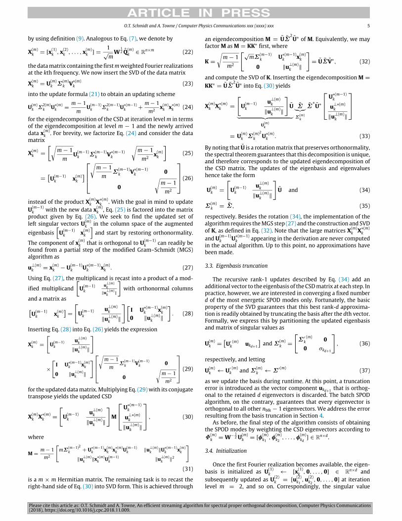
by using definition (9). Analogous to Eq. (7), we denote by

X(m)k

= [x(1)k

, x(2)k

, . . . , x(m)k

] =1pm

W12 Q

(m)k2 Rn⇥m (22)

the datamatrix containing the firstmweighted Fourier realizationsat the kth frequency. We now insert the SVD of the data matrix

X(m)k

= U(m)k

⌃ (m)k

V⇤(m)k

(23)

into the update formula (21) to obtain an updating scheme

U(m)k

⌃2(m)k

U⇤(m)k

=m� 1m

U(m�1)k

⌃2(m�1)k

U⇤(m�1)k

+m� 1m2 x

(m)k

x⇤(m)k

(24)

for the eigendecomposition of the CSD at iteration levelm in termsof the eigendecomposition at level m � 1 and the newly arriveddata x

(m)k

. For brevity, we factorize Eq. (24) and consider the datamatrix

X(m)k

=

rm� 1m

U(m�1)k

⌃ (m�1)k

V⇤(m�1)k

rm� 1m2 x

(m)k

�(25)

=⇥U

(m�1)k

x(m)k

⇤

2

664

rm� 1m

⌃ (m�1)k

V⇤(m�1)k

0

0

rm� 1m2

3

775 (26)

instead of the product X(m)k

X⇤(m)k

. With the goal in mind to updateU

(m�1)k

with the new data x(m)k

, Eq. (25) is factored into the matrixproduct given by Eq. (26). We seek to find the updated set ofleft singular vectors U

(m)k

in the column space of the augmentedeigenbasis

hU

(m�1)k

x(m)k

iand start by restoring orthonormality.

The component of x(m)k

that is orthogonal to U(m�1)k

can readily befound from a partial step of the modified Gram–Schmidt (MGS)algorithm as

u?(m)k

= x(m)k� U

(m�1)k

U⇤(m�1)k

x(m)k

. (27)

Using Eq. (27), the multiplicand is recast into a product of a mod-

ified multiplicandU

(m�1)k

u?(m)k

ku?(m)kk

�with orthonormal columns

and a matrix as⇥U

(m�1)k

x(m)k

⇤=

"U

(m�1)k

u?(m)k

ku?(m)kk

#I U

⇤(m�1)k

x(m)k

0 ku?(m)kk

�. (28)

Inserting Eq. (28) into Eq. (26) yields the expression

X(m)k

=

"U

(m�1)k

u?(m)k

ku?(m)kk

#

⇥

"I U

⇤(m�1)k

x(m)k

0 ku?(m)kk

#2

664

rm� 1m

⌃ (m�1)k

V(m�1)k

0

0

rm� 1m2

3

775 (29)

for the updated datamatrix.Multiplying Eq. (29)with its conjugatetranspose yields the updated CSD

X(m)k

X⇤(m)k

=

"U

(m�1)k

u?(m)k

ku?(m)kk

#M

2

64U⇤(m�1)k

u?⇤(m)k

ku?(m)kk

3

75 , (30)

where

M =m� 1m2

"m⌃ (m�1)2

k+ U

⇤(m�1)k

x(m)k

x⇤(m)k

U(m�1)k

ku?(m)kkU⇤(m�1)k

x(m)k

ku?(m)kkx⇤(m)k

U(m�1)k

ku?(m)kk2

#

(31)

is a m ⇥ m Hermitian matrix. The remaining task is to recast theright-hand side of Eq. (30) into SVD form. This is achieved through

an eigendecomposition M = U⌃2U⇤ of M. Equivalently, we may

factorM as M = KK⇤ first, where

K =

rm� 1m2

"pm⌃ (m�1)

kU⇤(m�1)k

x(m)k

0 ku?(m)kk

#= U⌃ V

⇤, (32)

and compute the SVD of K. Inserting the eigendecompositionM =

KK⇤ = U⌃

2U⇤ into Eq. (30) yields

X(m)k

X⇤(m)k

=

"U

(m�1)k

u?(m)k

ku?(m)kk

#U

| {z }U(m)k

⌃|{z}⌃ (m)

k

⌃⇤

U⇤

2

64U⇤(m�1)k

u?⇤(m)k

ku?(m)kk

3

75

= U(m)k

⌃ (m)2k

U⇤(m)k

. (33)

By noting that U is a rotationmatrix that preserves orthonormality,the spectral theoremguarantees that this decomposition is unique,and therefore corresponds to the updated eigendecomposition ofthe CSD matrix. The updates of the eigenbasis and eigenvalueshence take the form

U(m)k

=

"U

(m�1)k

u?(m)k

ku?(m)kk

#U and (34)

⌃ (m)k

= ⌃ , (35)

respectively. Besides the rotation (34), the implementation of thealgorithm requires theMGS step (27) and the construction and SVDof K, as defined in Eq. (32). Note that the large matrices X(m)

kX⇤(m)k

and U(m�1)k

U⇤(m�1)k

appearing in the derivation are never computedin the actual algorithm. Up to this point, no approximations havebeen made.

3.3. Eigenbasis truncation

The recursive rank-1 updates described by Eq. (34) add anadditional vector to the eigenbasis of the CSDmatrix at each step. Inpractice, however, we are interested in converging a fixed numberd of the most energetic SPOD modes only. Fortunately, the basicproperty of the SVD guarantees that this best rank-d approxima-tion is readily obtained by truncating the basis after the dth vector.Formally, we express this by partitioning the updated eigenbasisand matrix of singular values as

U(m)k

=⇥U0

k

(m)ukd+1

⇤and⌃ (m)

k=

"⌃ 0

k

(m)0

0 �kd+1

#, (36)

respectively, and letting

U(m)k U

0

k

(m) and⌃ (m)k ⌃ 0(m) (37)

as we update the basis during runtime. At this point, a truncationerror is introduced as the vector component ukd+1 that is orthog-onal to the retained d eigenvectors is discarded. The batch SPODalgorithm, on the contrary, guarantees that every eigenvector isorthogonal to all other nblk � 1 eigenvectors. We address the errorresulting from the basis truncation in Section 4.

As before, the final step of the algorithm consists of obtainingthe SPOD modes by weighting the CSD eigenvectors according to�(m)

k= W

�12 U

(m)k

= [�(m)k1

, �(m)k2

, . . . ,�(m)kd

] 2 Rn⇥d.

3.4. Initialization

Once the first Fourier realization becomes available, the eigen-basis is initialized as U

(1)k [x

(1)k

, 0, . . . , 0] 2 Rn⇥d andsubsequently updated as U

(2)k

= [u(2)k1

,u(2)k2

, 0, . . . , 0] at iterationlevel m = 2, and so on. Correspondingly, the singular value



matrix is initialized with the first Fourier realization as ⌃ (1)k

diag(x⇤(1)k

x(1)k

, 0, . . . , 0) 2 Rd⇥d before being updated as ⌃ (2)k

=

diag(� (2)k1

, �(2)k2

, 0, . . . , 0). The truncation of the eigenbasis is per-formed once the iteration level exceeds the number of desiredSPOD modes, i.e. whenm � d + 1.

Alternatively, the eigenbasis can be initialized fromapreviouslycomputed SPOD basis as U(1)

k= W

12�old

k. Initializing the algorithm

with an initial SPOD basis�oldk

obtained from a batch computationor a streaming computation with a larger value d has the benefit ofreducing the truncation error. This follows directly from the bestrank-d property of the SVD.

4. Errors and convergence

The errors of the approximation can be quantified by comparingthe rank-d solutions at themth iteration level to the reference solu-tion�batch

kand⌃ batch

kobtained from the batch algorithmdescribed

in Section 2.

Errors with respect to batch solution. We define two error quanti-ties

e�,batchj

(m) =

nfreqX

k=1

✓1�max

j

D�(m)kj

, �batchkj

E

E

◆and (38)

e�,batchj

(m) =

nfreqX

k=1

��(m)kj� �batch

kj

�batchkj

�� . (39)

that measure the error in the jth eigenvector and eigenvalue,respectively. The eigenvector error given by Eq. (38) is defined interms of the inner product (8) and compares the patterns of twomodes, i.e. it is 0 for identical and 1 for orthogonal modes. Themaximum over the mode rank index is taken to ensure that themost similar modes are compared to each other. This is importantas similar modes can swap order between iterations.

Convergence with respect to previous solution. Estimates for theconvergence of the eigenvectors and eigenvalues are defined anal-ogously in terms of their values at the previous iteration levelm�1.The resulting measures of convergence

e�,prevj

(m) =

nfreqX

k=1

✓1�max

j

D�(m)kj

, �(m�1)kj

E

E

◆and (40)

e�,prevj

(m) =

nfreqX

k=1

��(m)kj� �

(m�1)kj

�(m�1)kj

�� , (41)

for the jth eigenfunction and eigenvalue, respectively, can bemon-itored during runtime.

5. Examples

This section demonstrates the performance of the proposedstreaming SPOD algorithm on two examples. The first example isa high-fidelity numerical simulation of a turbulent jet [19], andthe second example is optical flow obtained from a high-speedmovie of a stepped spillway experiment [20,21]. Anoverviewof thedatabases and SPOD parameters is presented in Table 1. The SPODparameters are chosen according to best practice. A discussion ofhow to choose them is beyond the scope of this work. The sameapplies to detailed physical interpretations of the results. Here,we focus on the performance and convergence of the streamingalgorithm as compared to its offline batch counterpart. We usea Hanning window for the Fourier transformation and set thenumber of retained SPOD modes to d = 5. The effect of eigenbasistruncation is discussed in more detail in Section 6.

Table 1

Parameters for the two example databases and the SPOD. The spectral estimationparameters nfreq, novlp and nblk are identical for batch and streaming SPOD. d is thenumber of desired modes for the streaming algorithm.Database SPOD parametersCase q nx1 nx2 nt nfreq novlp nblk d

Jet psymm 175 39 10,000 256 128 78 5

Spillway [u, v] 224 160 19,782 512 256 77 5

5.1. Example 1: large eddy simulation of a turbulent jet

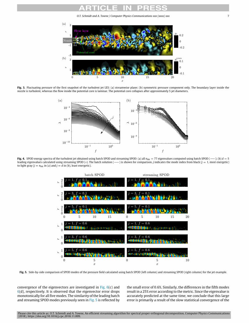
The turbulent jet is a typical examples of a stationary flow. Anumber of studies, see e.g. [22] for an early experimental and [23]for a recent numerical example, use SPOD to analyze jet turbulence.Our first is example is an LES of a Mach 0.9 jet at a jet diameter-based Reynolds number of 1.01 · 106 [19]. The LES was calculatedusing the unstructured flow solver ‘‘Charles" [24]. The databaseconsists of 10,000 snapshots of the axisymmetric component of thepressure field obtained as the zeroth azimuthal Fourier componentof the flow. We choose to resolve 129 positive frequencies bysetting nfreq = 256. Each block therefore consists of 256 snapshots.We further use a 50% overlap by letting novlp = 128. This resultsin a total of 77 blocks for the spectral estimation, each of whichrepresents one realization of the temporal Fourier transform. Thefirst snapshot of the database is visualized in Fig. 3. The chaoticnature of the flow becomes apparent at first glance.

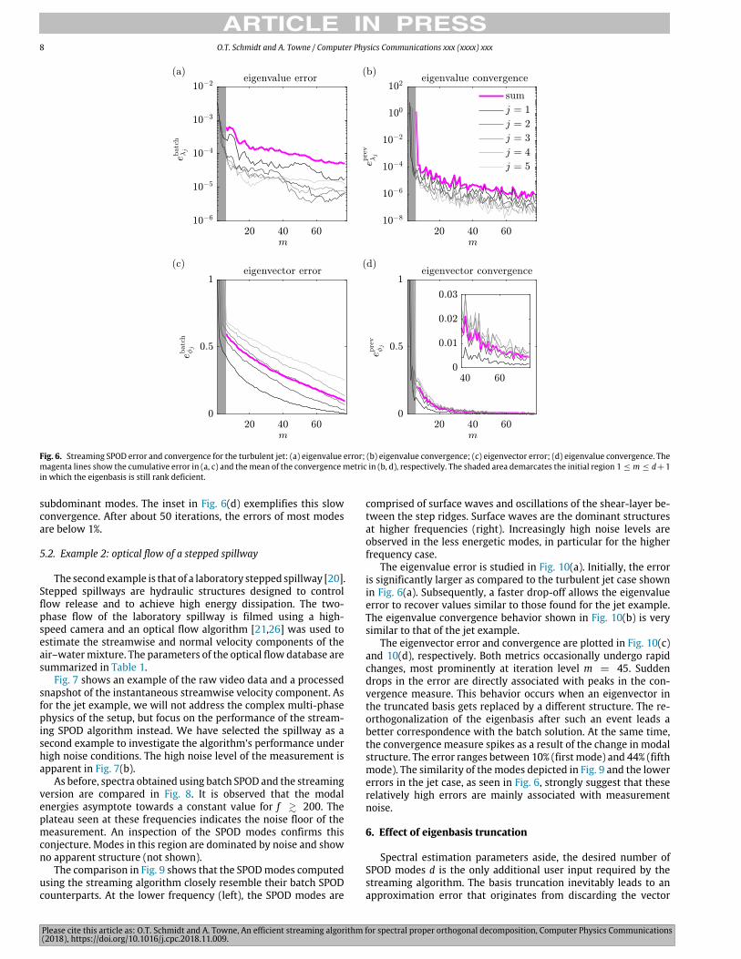
Fig. 4(a) shows the batch SPOD spectrum obtained for thespectral estimation parameters listed in Table 1. Each line repre-sents the energy spectrum associated with a single mode indexj. The total number of modes is equal to the number of blocks,i.e. nblk = 77 in this example. Most of the energy is concentratedin the large-scale structures that dominate at low frequencies. Theroll-off of the distribution at higher frequencies is indicative ofan energy cascade that transfers energy from larger to smallerscales. Over a certain frequency interval 0.1 . f . 0.6, the firstmode is significantly more energetic that the other modes. Thislow-rank behavior has important physical implications discussedelsewhere [25]. The spectra of the five leadingmodes are replicatedin Fig. 4(b) and compared to the results obtained using streamingSPOD (� symbols). It can be seen that the two results are almost in-distinguishable. This provides a first indication that the streamingSPOD algorithm accurately approximates the SPOD eigenvalues.We will quantify this observation in the context of Fig. 6.

After establishing that the modal energies are well approxi-mated by the streaming algorithm, we next examine the modalstructures. Fig. 5 shows a side-by-side comparison of the first (j =

1), third (j = 3) and fifth (j = 5) modes at two representativefrequencies (f = 0.1, top half and f = 0.6, bottom half). Theleading modes (first and fourth row) computed using streamingSPOD are almost indistinguishable from the reference solution forboth frequencies. The thirdmodes (second and fifth row) still com-parewell. More differences become apparent for the fifthmodes. Ithas to be kept in mind though, that the subdominant modes are ingeneralmore difficult to converge. This exemplifies the importanceof being able to converge second-order statistics from long datasequences.

In Fig. 6, we next investigate the errors and convergence be-havior for the jet example in terms of the quantities defined inEqs. (38)–(41). The eigenvalue error in Fig. 6(a) drops by approx-imately one order of magnitude from beginning to end. As an-ticipated from Fig. 4(b), the eigenvalue error is generally small,i.e. below the per mil range after the first iteration. The eigen-value convergence is addressed in Fig. 6(b). Starting from the endof the initialization phase (gray shaded area), the convergencemeasure drops by about two orders of magnitude. The error and



Fig. 3. Fluctuating pressure of the first snapshot of the turbulent jet LES: (a) streamwise plane; (b) symmetric pressure component only. The boundary layer inside thenozzle is turbulent, whereas the flow inside the potential core is laminar. The potential core collapses after approximately 5 jet diameters.

Fig. 4. SPOD energy spectra of the turbulent jet obtained using batch SPOD and streaming SPOD: (a) all nblk = 77 eigenvalues computed using batch SPOD (��); (b) d = 5leading eigenvalues calculated using streaming SPOD (�). The batch solution (��) is shown for comparison. j indicates the mode index from black (j = 1, most energetic)to light gray (j = nblk in (a) and j = d in (b), least energetic).

Fig. 5. Side-by-side comparison of SPOD modes of the pressure field calculated using batch SPOD (left column) and streaming SPOD (right column) for the jet example.

convergence of the eigenvectors are investigated in Fig. 6(c) and6(d), respectively. It is observed that the eigenvector error dropsmonotonically for all fivemodes. The similarity of the leading batchand streaming SPODmodes previously seen in Fig. 5 is reflected by

the small error of 0.6%. Similarly, the differences in the fifth modesresult in a 25% error according to themetric. Since the eigenvalue isaccurately predicted at the same time, we conclude that this largeerror is primarily a result of the slow statistical convergence of the



Fig. 6. Streaming SPOD error and convergence for the turbulent jet: (a) eigenvalue error; (b) eigenvalue convergence; (c) eigenvector error; (d) eigenvalue convergence. Themagenta lines show the cumulative error in (a, c) and themean of the convergencemetric in (b, d), respectively. The shaded area demarcates the initial region 1 m d+1in which the eigenbasis is still rank deficient.

subdominant modes. The inset in Fig. 6(d) exemplifies this slowconvergence. After about 50 iterations, the errors of most modesare below 1%.

5.2. Example 2: optical flow of a stepped spillway

The secondexample is that of a laboratory stepped spillway [20].Stepped spillways are hydraulic structures designed to controlflow release and to achieve high energy dissipation. The two-phase flow of the laboratory spillway is filmed using a high-speed camera and an optical flow algorithm [21,26] was used toestimate the streamwise and normal velocity components of theair–watermixture. The parameters of the optical flow database aresummarized in Table 1.

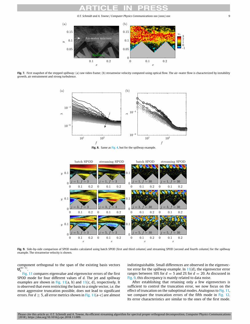
Fig. 7 shows an example of the raw video data and a processedsnapshot of the instantaneous streamwise velocity component. Asfor the jet example, we will not address the complex multi-phasephysics of the setup, but focus on the performance of the stream-ing SPOD algorithm instead. We have selected the spillway as asecond example to investigate the algorithm’s performance underhigh noise conditions. The high noise level of the measurement isapparent in Fig. 7(b).

As before, spectra obtained using batch SPOD and the streamingversion are compared in Fig. 8. It is observed that the modalenergies asymptote towards a constant value for f & 200. Theplateau seen at these frequencies indicates the noise floor of themeasurement. An inspection of the SPOD modes confirms thisconjecture. Modes in this region are dominated by noise and showno apparent structure (not shown).

The comparison in Fig. 9 shows that the SPODmodes computedusing the streaming algorithm closely resemble their batch SPODcounterparts. At the lower frequency (left), the SPOD modes are

comprised of surface waves and oscillations of the shear-layer be-tween the step ridges. Surface waves are the dominant structuresat higher frequencies (right). Increasingly high noise levels areobserved in the less energetic modes, in particular for the higherfrequency case.

The eigenvalue error is studied in Fig. 10(a). Initially, the erroris significantly larger as compared to the turbulent jet case shownin Fig. 6(a). Subsequently, a faster drop-off allows the eigenvalueerror to recover values similar to those found for the jet example.The eigenvalue convergence behavior shown in Fig. 10(b) is verysimilar to that of the jet example.

The eigenvector error and convergence are plotted in Fig. 10(c)and 10(d), respectively. Both metrics occasionally undergo rapidchanges, most prominently at iteration level m = 45. Suddendrops in the error are directly associated with peaks in the con-vergence measure. This behavior occurs when an eigenvector inthe truncated basis gets replaced by a different structure. The re-orthogonalization of the eigenbasis after such an event leads abetter correspondence with the batch solution. At the same time,the convergence measure spikes as a result of the change in modalstructure. The error ranges between 10% (firstmode) and 44% (fifthmode). The similarity of themodes depicted in Fig. 9 and the lowererrors in the jet case, as seen in Fig. 6, strongly suggest that theserelatively high errors are mainly associated with measurementnoise.

6. Effect of eigenbasis truncation

Spectral estimation parameters aside, the desired number ofSPOD modes d is the only additional user input required by thestreaming algorithm. The basis truncation inevitably leads to anapproximation error that originates from discarding the vector



Fig. 7. First snapshot of the stepped spillway: (a) raw video frame; (b) streamwise velocity computed using optical flow. The air–water flow is characterized by instabilitygrowth, air entrainment and strong turbulence.

Fig. 8. Same as Fig. 4, but for the spillway example.

Fig. 9. Side-by-side comparison of SPOD modes calculated using batch SPOD (first and third column) and streaming SPOD (second and fourth column) for the spillwayexample. The streamwise velocity is shown.

component orthogonal to the span of the existing basis vectorsU

(m�1)k

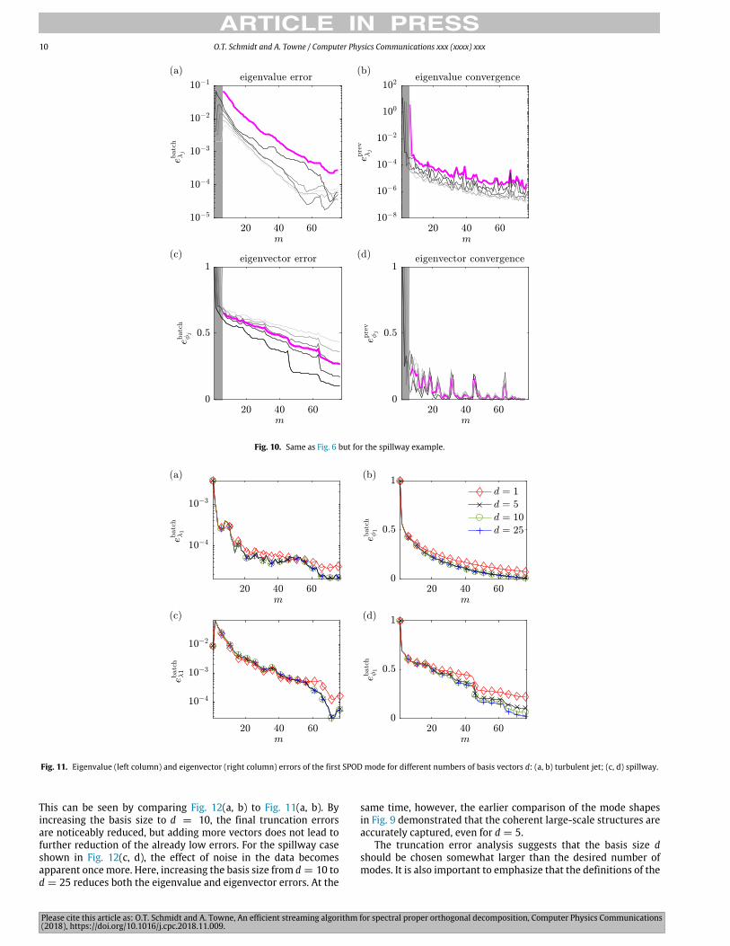
.Fig. 11 compares eigenvalue and eigenvector errors of the first

SPOD mode for four different values of d. The jet and spillwayexamples are shown in Fig. 11(a, b) and 11(c, d), respectively. Itis observed that even restricting the basis to a single vector, i.e. themost aggressive truncation possible, does not lead to significanterrors. For d � 5, all error metrics shown in Fig. 11(a–c) are almost

indistinguishable. Small differences are observed in the eigenvec-tor error for the spillway example. In 11(d), the eigenvector errorranges between 10% for d = 5 and 2% for d = 20. As discussed inFig. 9, this discrepancy is mainly related to data noise.

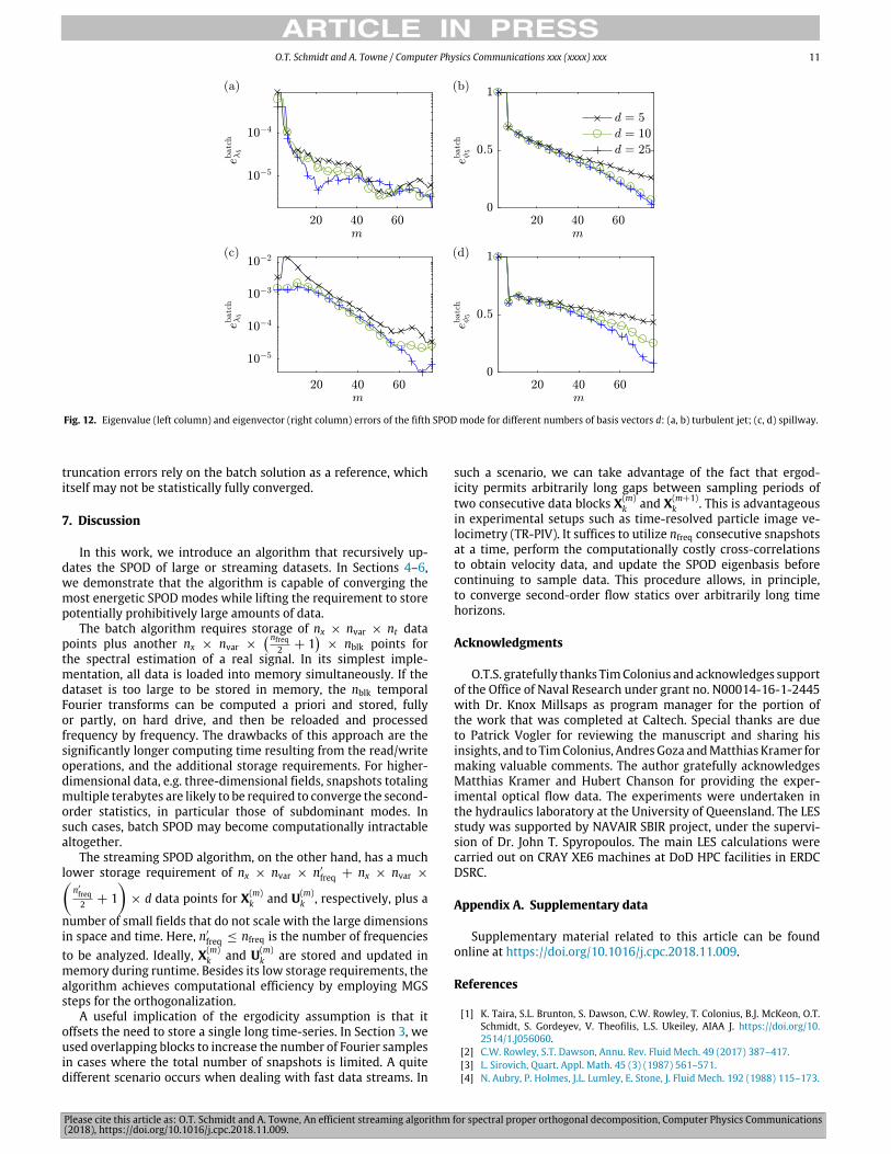
After establishing that retaining only a few eigenvectors issufficient to control the truncation error, we now focus on theeffect of truncation on the suboptimal modes. Analogous to Fig. 11,we compare the truncation errors of the fifth mode in Fig. 12.Its error characteristics are similar to the ones of the first mode.



Fig. 10. Same as Fig. 6 but for the spillway example.

Fig. 11. Eigenvalue (left column) and eigenvector (right column) errors of the first SPOD mode for different numbers of basis vectors d: (a, b) turbulent jet; (c, d) spillway.

This can be seen by comparing Fig. 12(a, b) to Fig. 11(a, b). Byincreasing the basis size to d = 10, the final truncation errorsare noticeably reduced, but adding more vectors does not lead tofurther reduction of the already low errors. For the spillway caseshown in Fig. 12(c, d), the effect of noise in the data becomesapparent oncemore. Here, increasing the basis size from d = 10 tod = 25 reduces both the eigenvalue and eigenvector errors. At the

same time, however, the earlier comparison of the mode shapesin Fig. 9 demonstrated that the coherent large-scale structures areaccurately captured, even for d = 5.

The truncation error analysis suggests that the basis size d

should be chosen somewhat larger than the desired number ofmodes. It is also important to emphasize that the definitions of the



Fig. 12. Eigenvalue (left column) and eigenvector (right column) errors of the fifth SPOD mode for different numbers of basis vectors d: (a, b) turbulent jet; (c, d) spillway.

truncation errors rely on the batch solution as a reference, whichitself may not be statistically fully converged.

7. Discussion

In this work, we introduce an algorithm that recursively up-dates the SPOD of large or streaming datasets. In Sections 4–6,we demonstrate that the algorithm is capable of converging themost energetic SPOD modes while lifting the requirement to storepotentially prohibitively large amounts of data.

The batch algorithm requires storage of nx ⇥ nvar ⇥ nt datapoints plus another nx ⇥ nvar ⇥

�nfreq2 + 1

�⇥ nblk points for

the spectral estimation of a real signal. In its simplest imple-mentation, all data is loaded into memory simultaneously. If thedataset is too large to be stored in memory, the nblk temporalFourier transforms can be computed a priori and stored, fullyor partly, on hard drive, and then be reloaded and processedfrequency by frequency. The drawbacks of this approach are thesignificantly longer computing time resulting from the read/writeoperations, and the additional storage requirements. For higher-dimensional data, e.g. three-dimensional fields, snapshots totalingmultiple terabytes are likely to be required to converge the second-order statistics, in particular those of subdominant modes. Insuch cases, batch SPOD may become computationally intractablealtogether.

The streaming SPOD algorithm, on the other hand, has a muchlower storage requirement of nx ⇥ nvar ⇥ n

0

freq + nx ⇥ nvar ⇥✓n0freq2 + 1

◆⇥ d data points for X(m)

kand U

(m)k

, respectively, plus a

number of small fields that do not scale with the large dimensionsin space and time. Here, n0freq nfreq is the number of frequenciesto be analyzed. Ideally, X(m)

kand U

(m)k

are stored and updated inmemory during runtime. Besides its low storage requirements, thealgorithm achieves computational efficiency by employing MGSsteps for the orthogonalization.

A useful implication of the ergodicity assumption is that itoffsets the need to store a single long time-series. In Section 3, weused overlapping blocks to increase the number of Fourier samplesin cases where the total number of snapshots is limited. A quitedifferent scenario occurs when dealing with fast data streams. In

such a scenario, we can take advantage of the fact that ergod-icity permits arbitrarily long gaps between sampling periods oftwo consecutive data blocks X(m)

kand X

(m+1)k

. This is advantageousin experimental setups such as time-resolved particle image ve-locimetry (TR-PIV). It suffices to utilize nfreq consecutive snapshotsat a time, perform the computationally costly cross-correlationsto obtain velocity data, and update the SPOD eigenbasis beforecontinuing to sample data. This procedure allows, in principle,to converge second-order flow statics over arbitrarily long timehorizons.

Acknowledgments

O.T.S. gratefully thanks TimColonius and acknowledges supportof the Office of Naval Research under grant no. N00014-16-1-2445with Dr. Knox Millsaps as program manager for the portion ofthe work that was completed at Caltech. Special thanks are dueto Patrick Vogler for reviewing the manuscript and sharing hisinsights, and to TimColonius, AndresGoza andMatthias Kramer formaking valuable comments. The author gratefully acknowledgesMatthias Kramer and Hubert Chanson for providing the exper-imental optical flow data. The experiments were undertaken inthe hydraulics laboratory at the University of Queensland. The LESstudy was supported by NAVAIR SBIR project, under the supervi-sion of Dr. John T. Spyropoulos. The main LES calculations werecarried out on CRAY XE6 machines at DoD HPC facilities in ERDCDSRC.

Appendix A. Supplementary data

Supplementary material related to this article can be foundonline at https://doi.org/10.1016/j.cpc.2018.11.009.

References

[1] K. Taira, S.L. Brunton, S. Dawson, C.W. Rowley, T. Colonius, B.J. McKeon, O.T.Schmidt, S. Gordeyev, V. Theofilis, L.S. Ukeiley, AIAA J. https://doi.org/10.2514/1.J056060.

[2] C.W. Rowley, S.T. Dawson, Annu. Rev. Fluid Mech. 49 (2017) 387–417.[3] L. Sirovich, Quart. Appl. Math. 45 (3) (1987) 561–571.[4] N. Aubry, P. Holmes, J.L. Lumley, E. Stone, J. Fluid Mech. 192 (1988) 115–173.



[5] B.R. Noack, K. Afanasiev, M.Morzy´ski, G. Tadmor, F. Thiele, J. FluidMech. 497(2003) 335–363.

[6] J.L. Lumley, New York, 1970.[7] A. Towne, O.T. Schmidt, T. Colonius, J. Fluid Mech. 847 (2018) 821–867, http:

//dx.doi.org/10.1017/jfm.2018.283.[8] P.J. Schmid, J. Fluid Mech. 656 (2010) 5–28, http://dx.doi.org/10.1017/

S0022112010001217.[9] M.S. Hemati, M.O.Williams, C.W. Rowley, Phys. Fluids 26 (11) (2014) 111701.

[10] H. Zhang, C.W. Rowley, E.A. Deem, L.N. Cattafesta, arXiv preprint arXiv:1707.02876.

[11] P. Businger, BIT 10 (3) (1970) 376–385.[12] R.D. De Groat, R.A. Roberts, in: Circuits, Systems and Computers, 1985. Nine-

teeth Asilomar Conference on, IEEE, 1985, pp. 601–605.[13] M. Brand, Linear Algebra Appl. 415 (1) (2006) 20–30.[14] M. Brand, Proc. Eur. Conf. Comput. Vis. (2002) 707–720.[15] M. Brand, in: Proceedings of the 2003 SIAM International Conference on Data

Mining, SIAM, 2003, pp. 37–46.

[16] P.D. Turney, P. Pantel, J. Artificial Intelligence Res. 37 (2010) 141–188.[17] T. Braconnier, M. Ferrier, J.-C. Jouhaud, M. Montagnac, P. Sagaut, Comput. &

Fluids 40 (1) (2011) 195–209.[18] O.M. Solomon Jr., NASA STI/Recon Technical Report N 92.[19] G.A. Brès, P. Jordan, V. Jaunet, M. Le Rallic, A.V.G. Cavalieri, A. Towne, S.K. Lele,

T. Colonius, O.T. Schmidt, J. Fluid Mech. 851 (2018) 83–124, http://dx.doi.org/10.1017/jfm.2018.476.

[20] M. Kramer, H. Chanson, Environ. Fluid Mech. (2018) 1–19.[21] G. Zhang, H. Chanson, Exp. Therm Fluid Sci. 90 (2017) (2017) 186–199.[22] M.N. Glauser, S.J. Leib, W.K. George, Turbul. Shear Flows 5 (1987) 134–145.[23] O.T. Schmidt, A. Towne, T. Colonius, A.V.G. Cavalieri, P. Jordan, G.A. Brès, J.

Fluid Mech. 825 (2017) 1153–1181, http://dx.doi.org/10.1017/jfm.2017.407.[24] G.A. Brès, F.E. Ham, J.W. Nichols, S.K. Lele, AIAA J. 55 (4) (2017) 1164–1184.[25] O.T. Schmidt, A. Towne, G. Rigas, T. Colonius, G.A. Brès, J. Fluid Mech. 855

(2018) 953–982, http://dx.doi.org/10.1017/jfm.2018.675.[26] T. Liu, A. Merat, M.H.M. Makhmalbaf, C. Fajardo, P. Merati, Exp. Fluids 56 (8)

(2015) 1–23.

Documents

An efficient streaming algorithm for spectral proper