An Embedded-Atom-Method Model for Alkali-Metal Vibrations Alkali Vibrations IOP.pdf · An Embedded-Atom-Method Model for Alkali-Metal Vibrations R B Wilson and D M Ri e ... Abstract

An Embedded-Atom-Method Model for

Alkali-Metal Vibrations

R B Wilson and D M Riffe

Physics Department, Utah State University, Logan, UT 84322-4415

Abstract. We present an embedded-atom-method (EAM) model that accurately

describes vibrational dynamics in the alkali metals Li, Na, K, Rb, and Cs. Bulk

dispersion curves, frequency-moment Debye temperatures, and temperature-dependent

entropy Debye temperatures are all in excellent agreement with experimental results.

The model is also well suited for studying surface vibrational dynamics in these

materials, as illustrated by calculations for the Na(110) surface.

PACS numbers: 63.20.dh, 68.35.Ja

1. Introduction

The embedded atom method (EAM), originally developed by Daw and Baskes to study

fcc metals [1, 2], is a semi-empirical, many-body approach that can be used to calculate

a wide variety of materials properties such as lattice stability, thermal expansion, surface

and interface structure, defect properties, and vibrational dynamics [3]. EAM models

have had particular success at predicting both bulk and surface phonons in fcc metals

such as Cu and Ag [3, 4, 5, 6, 7].

In contrast, many EAM models do a rather poor job of predicting the vibrational

properties of bcc metals, including the simple metals Li, Na, K, Rb, and Cs. This

can partly be ascribed to the longer range and/or angular nature of the forces in the

less closed packed bcc lattice, which makes appropriate EAM modeling more complex

than for fcc materials. The lack of success can also be ascribed, in some cases, to

the use of less-than-ideal input parameters in constructing the EAM potentials. There

are, however, a few encouraging counterexamples to this generally poor performance,

notably the EAM potentials of Chantasiriwan and Milstein (CM) for Li and K, which do

a relatively good job at predicting phonon dispersion for these two metals [8]. The CM

results suggest that the EAM has the potential to accurately describe the vibrational

properties of the alkali metals and also, perhaps, other bcc metals.

Here we present a normalized EAM model, based on the pair-potential formulation

of Wang and Boercker (WB) [9] and analytic embedding energy of Johnson and Oh

(JO) [10], that accurately predicts bulk vibrational properties associated with all of the

alkali metals. These properties include not only dispersion curves, but also frequency-

moment and vibrational-entropy Debye temperatures. The quantitative agreement that

Wilson and Riffe J. Phys.: Condens. Matter 24, 335401 (2012)

we obtain with experiment is superior to that obtained from other EAM treatments

of alkali-metal lattice dynamics. We also apply the model to the most studied allkali-

metal surface, Na(110). We identify surface localized modes and calculate directionally

resolved Debye temperatures for near-surface planes of atoms.

2. EAM model

The EAM describes the total potential energy associated with the atomic positions as

a sum of pair potentials ϕ(rij) and embedding energies F (ρi)

U =1

2

∑ij

ϕ(rij) +∑i

F (ρi), (1)

where i and j (i = j) label the atoms in the solid, rij is the distance between atoms i

and j, and ρi is the electron density at the position of atom i due to all of the other

atoms in the solid. It is assumed that this density can be written as a sum of individual

atomic densities f(rij)

ρi =∑j

f(rij). (2)

Specifying the functions ϕ(r), F (ρ), and f(r) establishes an EAM model for a particular

material.

To describe the alkali metals we use previously introduced forms for these three

functions. Our choices for these functions are predicated on the ability of the resulting

models to (i) accurately describe bulk-phonon spectra and (ii) produce realistic values

for surface relaxation. Both abilities are necessary for accurately predicting surface

phonons. After considering a number of potential functions we settled on the pair-

potential formulation of WB [9],

ϕ(r) =6∑

n=0

Kn

(r

r1− 1

)n

exp

(−nα

(r

r1− 1

)2), (3)

and the embedding-energy functions of JO [10, 11],

F (ρ) = −(Ecoh − EUF

1v

) [1− λ ln

(ρ

ρe

)](ρ

ρe

)λ

(4)

and

f(r) = f1 exp(−β

(r

r1− 1

)). (5)

In (3) – (5) the parameter r1 is the nearest-neighbor distance, Ecoh the cohesive energy,

and EUF1v the (unrelaxed) vacancy formation energy; all are obtained from experimental

measurements. The parameters Kn in (3) are also determined from experimental inputs,

as described below. The exact value of the nearest-neighbor density f1 in (4) does not

impact the model because the embedding function F (ρ) only depends upon the ratio

2


of the charge density ρ to its equilibrium value ρe; for simplicity we set its value to 1.

Following JO we choose β to have the value of 6 [10]. Because F (ρ) is a minimum at

the equilibrium density ρe, this model is known as a normalized EAM model.

Following WB [9], we determine the seven pair-potential parametersKn in (3) using

0 = 4r1ϕ′1 + 3r2ϕ

′2 + 6r3ϕ

′3 + 12r4ϕ

′4 + 4r5ϕ

′5, (6)

15ΩG = 4r21 (ϕ′′1 + ϕ′′

2 + 4ϕ′′3 + 11ϕ′′

4 + 4ϕ′′5) , (7)

3ΩC ′ = 2r21

(ϕ′′2 −

ϕ′2

r2+ ϕ′′

3 −ϕ′3

r3+

64

11ϕ′′4 −

64

11

ϕ′4

r4

), (8)

EUF1v = −4ϕ1 − 3ϕ2 − 6ϕ3 − 12ϕ4 − 4ϕ5, (9)

3

16Mω2

100 = ϕ′′1 + 2

ϕ′1

r1+ 3ϕ′′

4 + 6ϕ′4

r4, (10)

1

4Mω2

12

120 =

4

3ϕ′′1 +

2

3

ϕ′1

r1+ ϕ′′

2 +ϕ′2

r2+ ϕ′′

3 + 3ϕ′3

r3+

12

11ϕ′′4 +

54

11

ϕ′4

r4, (11)

and

3

8Mω2

12

12

12= ϕ′′

1 + 2ϕ′1

r1+

3

2ϕ′′2 + 3

ϕ′2

r2+ 3ϕ′′

4 + 6ϕ′4

r4+ 2ϕ′′

5 + 4ϕ′5

r5. (12)

In these equations ϕ′i = dϕ/dr and ϕ′′

i = d2ϕ/dr2 evaluated at ri, where ri is the

equilibrium distance to the i th shell of neighbors. In addition to the vacancy formation

energy EUF1v , experimental inputs to these equations are the atomic mass M , atomic

volume Ω = a30/2 (a0 = lattice constant), elastic constants G = (C11 − C12 + 3C44)/5

and C ′ = (C11 − C12)/2, and three longitudinal-mode (angular) frequencies ωijk, where

the subscript denotes the location of the mode at the boundary of the Brillouin zone

(BZ). As is evident in (6) – (12) the pair potential for neighbors beyond the fifth shell

is assumed to be zero. A simple scheme can be used to smoothly cut off the potential,

as expressed by (3), between the fifth and sixth neighbor distances [12]. Similarly, f(r)

is assumed to smoothly go to zero for r between r5 and r6.

We determine the best values for the exponents λ and α by comparing calculated

and experimental dispersion curves (discussed in detail in section 3). Surface relaxation

(see section 4.1) is also considered in choosing λ. This approach differs from that

of JO, who use a universal value, λ =√1/8 (= 0.354), based on a comparison of

their model with early first-principles calculations of the atomic potentials [10]. This

is fairly close to our values for Li and Na. However, we find that λ = 0.354 results

in [100] longitudinal frequencies for K, Rb, and Cs that are significantly smaller than

the experimental measurements. We also note that our values of α for all of the alkali

metals (which are all close to 0.5) contrast with the choice made by WB, who set α = 0

for their modeling of Li, Na, and K [9].

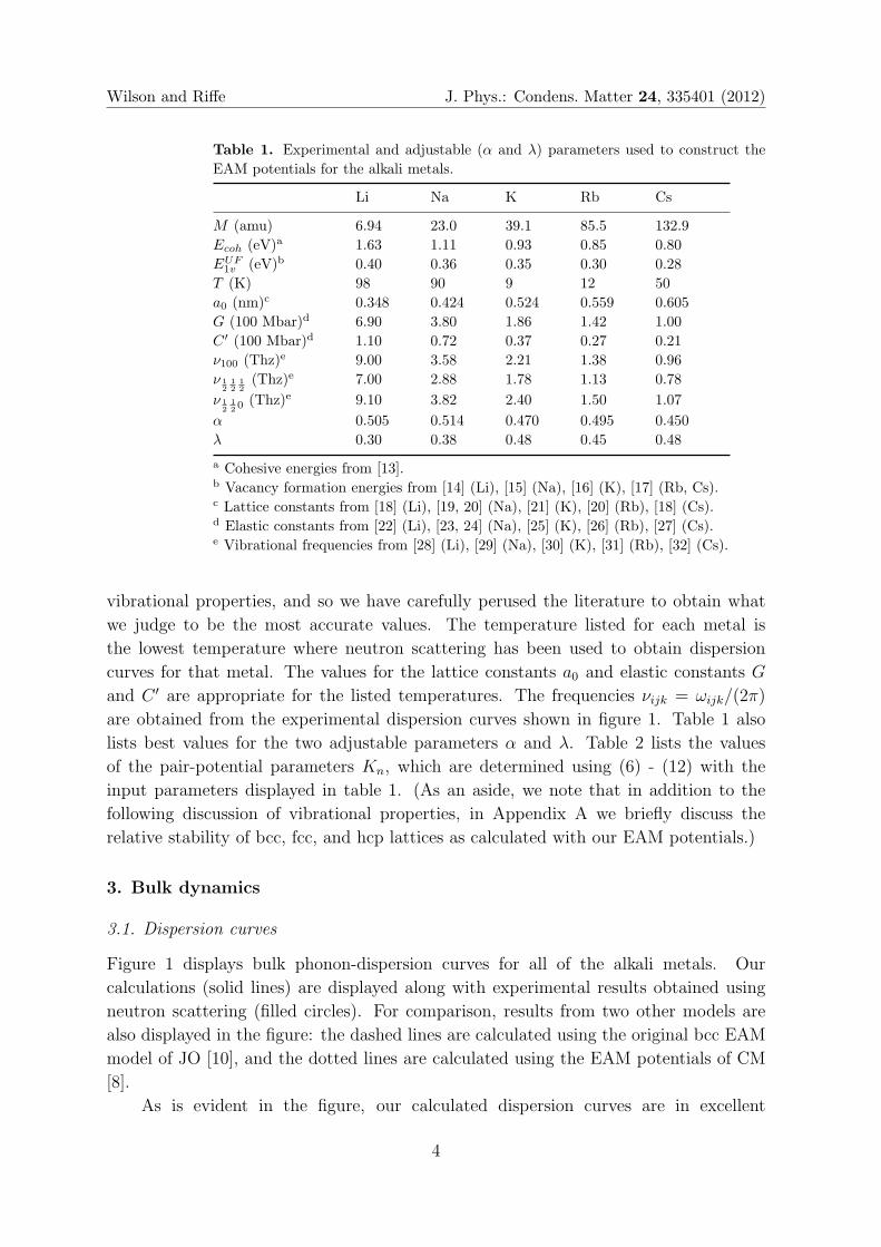
Table 1 lists values of the experimental parameters that we have used to construct

the EAM potentials for the alkali metals. We emphasize that accurate values of

the experimentally determined parameters are crucial in order to successfully predict

3


Table 1. Experimental and adjustable (α and λ) parameters used to construct the

EAM potentials for the alkali metals.

Li Na K Rb Cs

M (amu) 6.94 23.0 39.1 85.5 132.9

Ecoh (eV)a 1.63 1.11 0.93 0.85 0.80

EUF1v (eV)b 0.40 0.36 0.35 0.30 0.28

T (K) 98 90 9 12 50

a0 (nm)c 0.348 0.424 0.524 0.559 0.605

G (100 Mbar)d 6.90 3.80 1.86 1.42 1.00

C ′ (100 Mbar)d 1.10 0.72 0.37 0.27 0.21

ν100 (Thz)e 9.00 3.58 2.21 1.38 0.96

ν 12

12

12(Thz)e 7.00 2.88 1.78 1.13 0.78

ν 12

120

(Thz)e 9.10 3.82 2.40 1.50 1.07

α 0.505 0.514 0.470 0.495 0.450

λ 0.30 0.38 0.48 0.45 0.48

a Cohesive energies from [13].b Vacancy formation energies from [14] (Li), [15] (Na), [16] (K), [17] (Rb, Cs).c Lattice constants from [18] (Li), [19, 20] (Na), [21] (K), [20] (Rb), [18] (Cs).d Elastic constants from [22] (Li), [23, 24] (Na), [25] (K), [26] (Rb), [27] (Cs).e Vibrational frequencies from [28] (Li), [29] (Na), [30] (K), [31] (Rb), [32] (Cs).

vibrational properties, and so we have carefully perused the literature to obtain what

we judge to be the most accurate values. The temperature listed for each metal is

the lowest temperature where neutron scattering has been used to obtain dispersion

curves for that metal. The values for the lattice constants a0 and elastic constants G

and C ′ are appropriate for the listed temperatures. The frequencies νijk = ωijk/(2π)

are obtained from the experimental dispersion curves shown in figure 1. Table 1 also

lists best values for the two adjustable parameters α and λ. Table 2 lists the values

of the pair-potential parameters Kn, which are determined using (6) - (12) with the

input parameters displayed in table 1. (As an aside, we note that in addition to the

following discussion of vibrational properties, in Appendix A we briefly discuss the

relative stability of bcc, fcc, and hcp lattices as calculated with our EAM potentials.)

3. Bulk dynamics

3.1. Dispersion curves

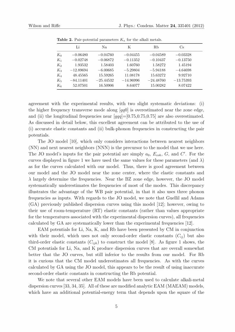
Figure 1 displays bulk phonon-dispersion curves for all of the alkali metals. Our

calculations (solid lines) are displayed along with experimental results obtained using

neutron scattering (filled circles). For comparison, results from two other models are

also displayed in the figure: the dashed lines are calculated using the original bcc EAM

model of JO [10], and the dotted lines are calculated using the EAM potentials of CM

[8].

As is evident in the figure, our calculated dispersion curves are in excellent

4


Table 2. Pair-potential parameters Kn for the alkali metals.

Li Na K Rb Cs

K0 −0.06480 −0.04760 −0.04455 −0.04589 −0.03328

K1 −0.02748 −0.06872 −0.11352 −0.10437 −0.13750

K2 1.93532 1.58403 1.60760 1.58272 1.45194

K3 −12.89694 −6.00685 −5.29804 −5.94188 −4.64698

K4 48.45565 15.59265 11.08178 15.63272 9.92710

K5 −84.11401 −25.44532 −14.96996 −24.48760 −13.75393

K6 52.07501 16.50906 8.64077 15.00282 8.07422

agreement with the experimental results, with two slight systematic deviations: (i)

the higher frequency transverse mode along [qq0] is overestimated near the zone edge,

and (ii) the longitudinal frequencies near [qqq]=[0.75,0.75,0.75] are also overestimated.

As discussed in detail below, this excellent agreement can be attributed to the use of

(i) accurate elastic constants and (ii) bulk-phonon frequencies in constructing the pair

potentials.

The JO model [10], which only considers interactions between nearest neighbors

(NN) and next nearest neighbors (NNN) is the precursor to the model that we use here.

The JO model’s inputs for the pair potential are simply a0, Ecoh, G, and C ′. For the

curves displayed in figure 1 we have used the same values for these parameters (and λ)

as for the curves calculated with our model. Thus, there is good agreement between

our model and the JO model near the zone center, where the elastic constants and

λ largely determine the frequencies. Near the BZ zone edge, however, the JO model

systematically underestimates the frequencies of most of the modes. This discrepancy

illustrates the advantage of the WB pair potential, in that it also uses three phonon

frequencies as inputs. With regards to the JO model, we note that Guellil and Adams

(GA) previously published dispersion curves using this model [12]; however, owing to

their use of room-temperature (RT) elastic constants (rather than values appropriate

for the temperatures associated with the experimental dispersion curves), all frequencies

calculated by GA are systematically lower than the experimental frequencies [12].

EAM potentials for Li, Na, K, and Rb have been presented by CM in conjunction

with their model, which uses not only second-order elastic constants (Cij) but also

third-order elastic constants (Cijk) to construct the model [8]. As figure 1 shows, the

CM potentials for Li, Na, and K produce dispersion curves that are overall somewhat

better that the JO curves, but still inferior to the results from our model. For Rb

it is curious that the CM model underestimates all frequencies. As with the curves

calculated by GA using the JO model, this appears to be the result of using inaccurate

second-order elastic constants in constructing the Rb potential.

We note that several other EAM models have been used to calculate alkali-metal

dispersion curves [33, 34, 35]. All of these are modified analytic EAM (MAEAM) models,

which have an additional potential-energy term that depends upon the square of the

5


Figure 1. Bulk alkali-metal phonon-dispersion curves. Filled circles are experimental

data, [28] (Li), [29] (Na), [30] (K), [31] (Rb), [32] (Cs). Solid, dashed, and dotted lines

are present, JO, and CM EAM model calculations, respectively. See text for details.

electron density. The MAEAM model discussed by Hu and Masahiro (HM) produces

results similar to the those of the CM model [33]. Zhang and coworkers have published

two sets of dispersion curves based on the MAEAM approach; overall, the degree of

agreement with experiment is comparable to that of the JO-model calculated curves

displayed in figure 1 [34, 35].

6


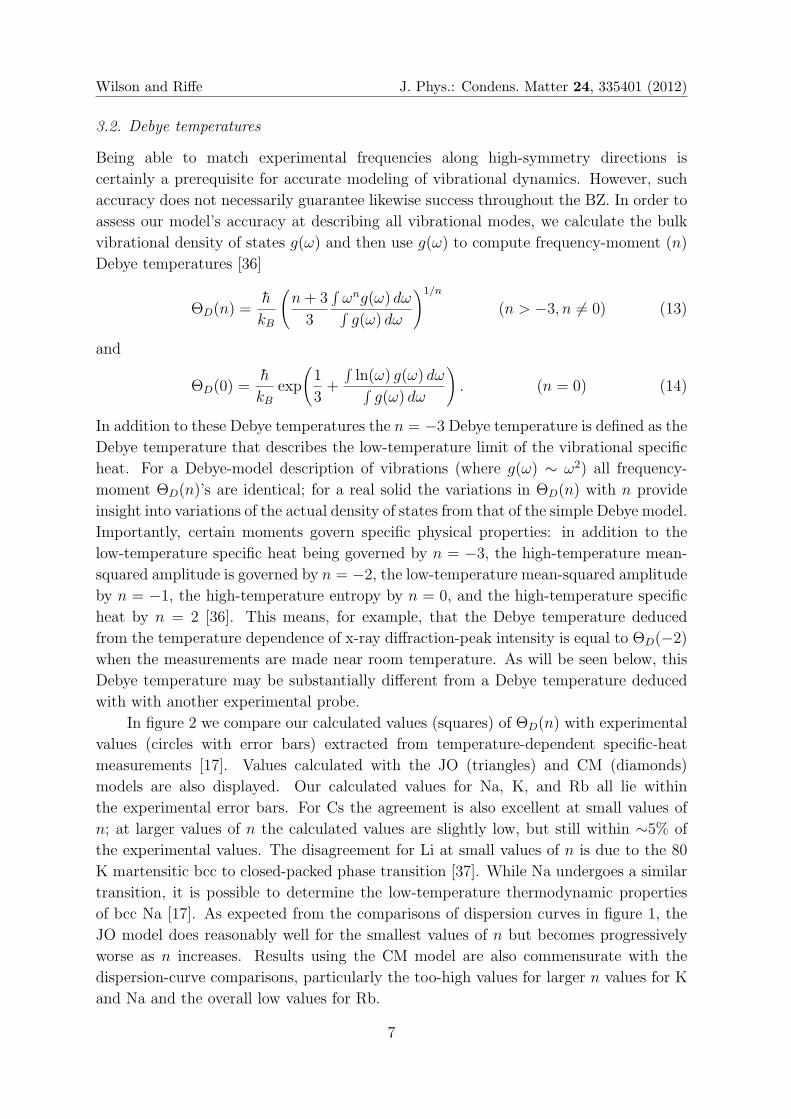
3.2. Debye temperatures

Being able to match experimental frequencies along high-symmetry directions is

certainly a prerequisite for accurate modeling of vibrational dynamics. However, such

accuracy does not necessarily guarantee likewise success throughout the BZ. In order to

assess our model’s accuracy at describing all vibrational modes, we calculate the bulk

vibrational density of states g(ω) and then use g(ω) to compute frequency-moment (n)

Debye temperatures [36]

ΘD(n) =h

kB

(n+ 3

3

∫ωng(ω) dω∫g(ω) dω

)1/n

(n > −3, n = 0) (13)

and

ΘD(0) =h

kBexp

(1

3+

∫ln(ω) g(ω) dω∫

g(ω) dω

). (n = 0) (14)

In addition to these Debye temperatures the n = −3 Debye temperature is defined as the

Debye temperature that describes the low-temperature limit of the vibrational specific

heat. For a Debye-model description of vibrations (where g(ω) ∼ ω2) all frequency-

moment ΘD(n)’s are identical; for a real solid the variations in ΘD(n) with n provide

insight into variations of the actual density of states from that of the simple Debye model.

Importantly, certain moments govern specific physical properties: in addition to the

low-temperature specific heat being governed by n = −3, the high-temperature mean-

squared amplitude is governed by n = −2, the low-temperature mean-squared amplitude

by n = −1, the high-temperature entropy by n = 0, and the high-temperature specific

heat by n = 2 [36]. This means, for example, that the Debye temperature deduced

from the temperature dependence of x-ray diffraction-peak intensity is equal to ΘD(−2)

when the measurements are made near room temperature. As will be seen below, this

Debye temperature may be substantially different from a Debye temperature deduced

with with another experimental probe.

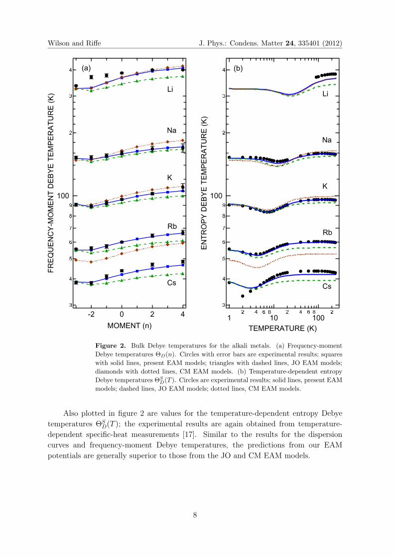
In figure 2 we compare our calculated values (squares) of ΘD(n) with experimental

values (circles with error bars) extracted from temperature-dependent specific-heat

measurements [17]. Values calculated with the JO (triangles) and CM (diamonds)

models are also displayed. Our calculated values for Na, K, and Rb all lie within

the experimental error bars. For Cs the agreement is also excellent at small values of

n; at larger values of n the calculated values are slightly low, but still within ∼5% of

the experimental values. The disagreement for Li at small values of n is due to the 80

K martensitic bcc to closed-packed phase transition [37]. While Na undergoes a similar

transition, it is possible to determine the low-temperature thermodynamic properties

of bcc Na [17]. As expected from the comparisons of dispersion curves in figure 1, the

JO model does reasonably well for the smallest values of n but becomes progressively

worse as n increases. Results using the CM model are also commensurate with the

dispersion-curve comparisons, particularly the too-high values for larger n values for K

and Na and the overall low values for Rb.

7


Figure 2. Bulk Debye temperatures for the alkali metals. (a) Frequency-moment

Debye temperatures ΘD(n). Circles with error bars are experimental results; squares

with solid lines, present EAM models; triangles with dashed lines, JO EAM models;

diamonds with dotted lines, CM EAM models. (b) Temperature-dependent entropy

Debye temperatures ΘSD(T ). Circles are experimental results; solid lines, present EAM

models; dashed lines, JO EAM models; dotted lines, CM EAM models.

Also plotted in figure 2 are values for the temperature-dependent entropy Debye

temperatures ΘSD(T ); the experimental results are again obtained from temperature-

dependent specific-heat measurements [17]. Similar to the results for the dispersion

curves and frequency-moment Debye temperatures, the predictions from our EAM

potentials are generally superior to those from the JO and CM EAM models.

8


4. Surface dynamics

4.1. Surface relaxation

Because the localization of vibrational modes at a surface can be quite sensitive to

structure, it is desirable that any theory used to calculate surface vibrations be able to

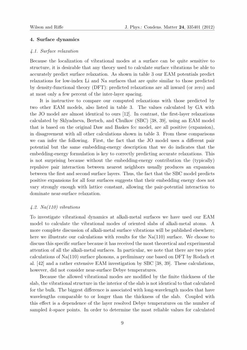
accurately predict surface relaxation. As shown in table 3 our EAM potentials predict

relaxations for low-index Li and Na surfaces that are quite similar to those predicted

by density-functional theory (DFT): predicted relaxations are all inward (or zero) and

at most only a few percent of the inter-layer spacing.

It is instructive to compare our computed relaxations with those predicted by

two other EAM models, also listed in table 3. The values calculated by GA with

the JO model are almost identical to ours [12]. In contrast, the first-layer relaxations

calculated by Sklyadneva, Bertsch, and Chulkov (SBC) [38, 39], using an EAM model

that is based on the original Daw and Baskes fcc model, are all positive (expansion),

in disagreement with all other calculations shown in table 3. From these comparisons

we can infer the following. First, the fact that the JO model uses a different pair

potential but the same embedding-energy description that we do indicates that the

embedding-energy formulation is key to correctly predicting accurate relaxations. This

is not surprising because without the embedding-energy contribution the (typically)

repulsive pair interaction between nearest neighbors usually produces an expansion

between the first and second surface layers. Thus, the fact that the SBC model predicts

positive expansions for all four surfaces suggests that their embedding energy does not

vary strongly enough with lattice constant, allowing the pair-potential interaction to

dominate near-surface relaxation.

4.2. Na(110) vibrations

To investigate vibrational dynamics at alkali-metal surfaces we have used our EAM

model to calculate the vibrational modes of oriented slabs of alkali-metal atoms. A

more complete discussion of alkali-metal surface vibrations will be published elsewhere;

here we illustrate our calculations with results for the Na(110) surface. We choose to

discuss this specific surface because it has received the most theoretical and experimental

attention of all the alkali-metal surfaces. In particular, we note that there are two prior

calculations of Na(110) surface phonons, a preliminary one based on DFT by Rodach et

al. [42] and a rather extensive EAM investigation by SBC [38, 39]. These calculations,

however, did not consider near-surface Debye temperatures.

Because the allowed vibrational modes are modified by the finite thickness of the

slab, the vibrational structure in the interior of the slab is not identical to that calculated

for the bulk. The biggest difference is associated with long-wavelength modes that have

wavelengths comparable to or longer than the thickness of the slab. Coupled with

this effect is a dependence of the layer resolved Debye temperatures on the number of

sampled k-space points. In order to determine the most reliable values for calculated

9


Table 3. Surface relaxations of Li and Na low-index surfaces. Negative (positive)

values signify inward (outward) relaxation. Values are the percentage of the interlayer

spacing for a given surface. ∆ij represents the change in distance (compared to the

bulk) between layers i and j.

Surface ∆12(%) ∆23(%) Technique

Li(110) −0.5 DFT b

−1.9 −0.06 EAM (present calculation)

−2.1 −0.08 EAM (GA) e

1.3 0.0 EAM (SBC) f

Na(110) 0 DFT a

0 DFT b

−1.6±0.5 0.0±0.5 DFT c


−1.5 −0.07 EAM (GA) e

2.4 0.1 EAM (SBC) f

Li(100) −3.0 DFT b


−2.6 −0.88 EAM (GA) e

5.3 0 EAM (SBC) f

Na(100) −2.0 DFT a

−0.7 DFT b

0 DFT d


−0.34 −0.91 EAM (GA) e

8.6 0.7 EAM (SBC) f

a[40].b[41].c[42].d[43].e[12].f [38, 39].

Debye temperatures we have thus investigated their dependence on these two factors. We

find for 1600 sampled k-space points that a slab thickness 30 times the lattice constant

is sufficient to produce n ≥ −2 center-layer Debye temperatures that are within 5%

of bulk Debye temperatures, which we set as our criterion for accuracy. We note that

because they are extremely sensitive to the longest wavelength modes, n = −3 Debye

temperatures cannot be accurately calculated in a slab geometry with a reasonable

number of layers and sampled k-space points.

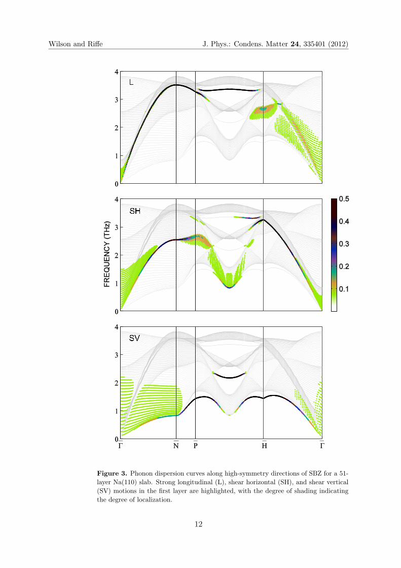
Dispersion curves for Na(110) along high-symmetry directions in the surface

Brillouin zone (SBZ) are shown in figure 3 for a 51 layer slab. The three panels of

this figure highlight strong longitudinal (L), shear horizontal (SH), and shear vertical

(SV) motions in the first layer with the degree of localization indicated by the degree

10


of the shading. Strongly localized modes of all three symmetry types are found at this

surface.

Although there is general overall qualitative agreement with vibrational spectra

previously calculated by SBC using their EAM model [38, 39], the results shown in figure

3 have several notable differences. (i) The range of frequencies for a given wavevector are

much smaller for our model than for the SBC model. For example, at N our calculated

frequencies range from 0.8 to 3.8 THz while those of the SBC model range from 0.3

to 4.5 THz. These differences are a consequence of the SBC model underestimating

and overestimating the lowest and highest frequencies, respectively, along the bulk [110]

direction [39]. (ii) The strong SH mode in the Γ to H direction was not identified

by SBC. (iii) In the Γ to N direction the Rayleigh mode in the SBC calculation is

significantly below the bottom of the bulk bands. For example, at N SBC calculate the

Rayleigh-mode frequency to be about half that of the lowest bulk mode. In contrast,

along Γ to N our calculation predicts the Rayleigh mode to be just below the bulk

bands. Observations (ii) and (iii) are likely related to the unphysical outward expansion

of the first layer in the SBC model (see table 3).

Our calculated vibrational structure also has significant differences compared with

results from the early DFT calculations of Rodach et al. [42]. The main differences

in the spectra of Rodach et al. are (i) the absence of a first-layer longitudinal mode

between P and H below the highest part of the bulk spectrum and (ii) the presence of

a surface-localized mode above much of the bulk spectrum. These differences can be

traced to a significant stiffening (compared to the bulk) of the surface force constants

in the Rodach et al. model.

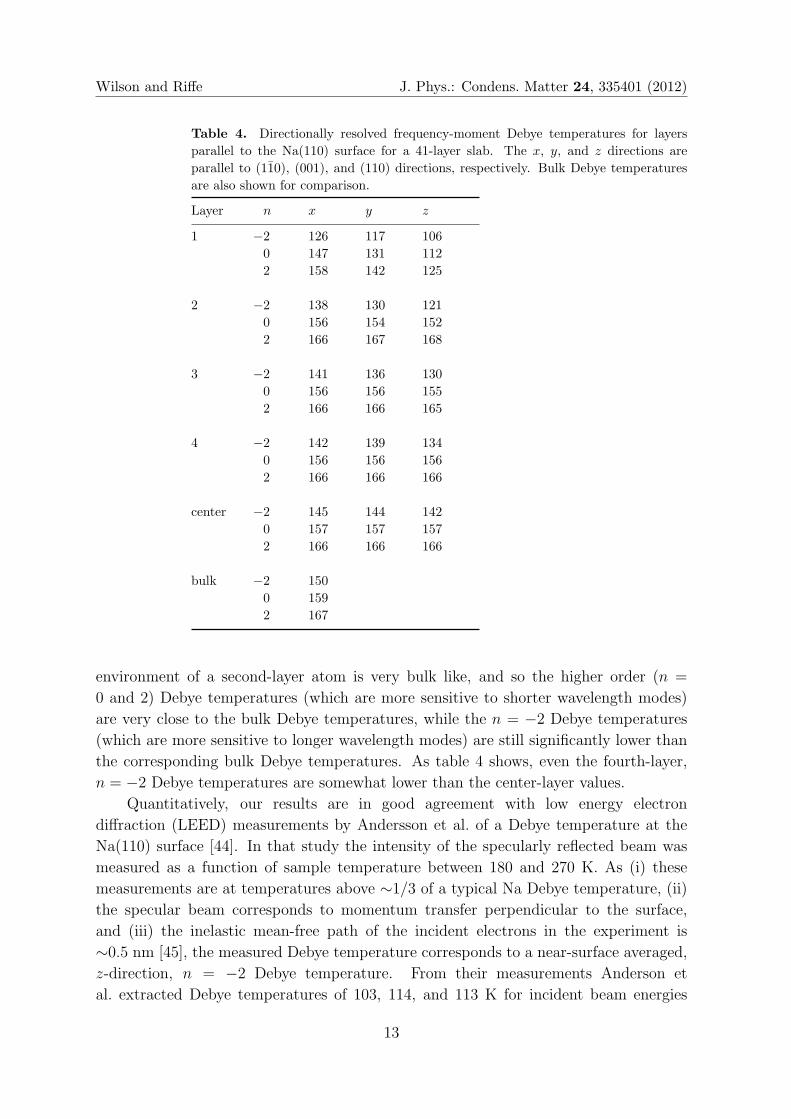
Further insight into near-surface vibrational dynamics is provided by layer resolved

Debye temperatures, which are listed in table 4 for n = −2, 0, and 2. Also listed are

results for the center layer and results obtained from the bulk calculation. In addition to

being layer resolved, the tabulated Debye temperatures are resolved for motions parallel

(x and y) and perpendicular (z) to the surface normal. Because the n = −2 Debye

temperatures are most sensitive to longer wavelength modes, the center-layer values do

not converge as readily to the bulk value as do the n = 0 and 2 values, although all are

within 5% of the bulk values.

The major qualitative aspects of the near-surface Debye temperatures can be

understood by considering the coordination of the atoms in each layer. As table 4 shows,

the Debye temperatures of the first atomic layer are all less than the corresponding Debye

temperatures of deeper layers, and motion perpendicular to the surface is softer than

parallel motion. The relative overall softness of the vibrations in the first layer is not

unexpected as a first-layer atom is missing 2 of 8 nearest neighbor (NN) atoms and 2 of

6 next-nearest neighbor (NNN) atoms. The first-layer directional dependence can also

be understood in terms of coordination as a first-layer atom has the same intralayer NN

and NNN coordinations as a bulk atom, but is missing half of its out-of-layer nearest

and next-nearest neighbors. For the bcc(110) surface a second-layer atom is coordinated

by all of its nearest and next-nearest neighbors. Thus, on the length scale of ∼2a0 the

11


Figure 3. Phonon dispersion curves along high-symmetry directions of SBZ for a 51-

layer Na(110) slab. Strong longitudinal (L), shear horizontal (SH), and shear vertical

(SV) motions in the first layer are highlighted, with the degree of shading indicating

the degree of localization.

12


Table 4. Directionally resolved frequency-moment Debye temperatures for layers

parallel to the Na(110) surface for a 41-layer slab. The x, y, and z directions are

parallel to (110), (001), and (110) directions, respectively. Bulk Debye temperatures

are also shown for comparison.

Layer n x y z

1 −2 126 117 106

0 147 131 112

2 158 142 125

2 −2 138 130 121

0 156 154 152

2 166 167 168

3 −2 141 136 130

0 156 156 155

2 166 166 165

4 −2 142 139 134

0 156 156 156

2 166 166 166

center −2 145 144 142

0 157 157 157

2 166 166 166

bulk −2 150

0 159

2 167

environment of a second-layer atom is very bulk like, and so the higher order (n =

0 and 2) Debye temperatures (which are more sensitive to shorter wavelength modes)

are very close to the bulk Debye temperatures, while the n = −2 Debye temperatures

(which are more sensitive to longer wavelength modes) are still significantly lower than

the corresponding bulk Debye temperatures. As table 4 shows, even the fourth-layer,

n = −2 Debye temperatures are somewhat lower than the center-layer values.

Quantitatively, our results are in good agreement with low energy electron

diffraction (LEED) measurements by Andersson et al. of a Debye temperature at the

Na(110) surface [44]. In that study the intensity of the specularly reflected beam was

measured as a function of sample temperature between 180 and 270 K. As (i) these

measurements are at temperatures above ∼1/3 of a typical Na Debye temperature, (ii)

the specular beam corresponds to momentum transfer perpendicular to the surface,

and (iii) the inelastic mean-free path of the incident electrons in the experiment is

∼0.5 nm [45], the measured Debye temperature corresponds to a near-surface averaged,

z-direction, n = −2 Debye temperature. From their measurements Anderson et

al. extracted Debye temperatures of 103, 114, and 113 K for incident beam energies

13


of 14, 35.5 and 65.5 eV, respectively. These values are all very close to the average

value (113.5 K) of our calculated first and second layer n = −2, z-direction Debye

temperatures.

5. Summary

We have presented results for alkali-metal vibrational dynamics calculated with an

analytic EAM model. Keys to the construction of the EAM potentials include (i) the use

of the best available physical parameters (elastic constants, vibrational frequencies, etc.),

(ii) a careful search for the best value of the pair-potential free parameter α, and (iii)

consideration of surface relaxation in setting the value of the embedding-energy exponent

λ. As we have demonstrated, this model is able to accurately model bulk dispersion

curves, frequency-moment Debye temperatures, and (temperature dependent) entropy

Debye temperatures of all five alkali metals.

Given the model’s accurate descriptions of bulk-phonon spectra and surface

relaxation, we expect it to be able to accurately describe surface vibrations. We have

illustrated this ability with calculations of vibrations at the Na(110) surface. The

surface-phonon dispersion curves show significant differences when compared with other

calculations of this surface. Satisfyingly, the near-surface n = −2, perpendicular Debye

temperature is in excellent agreement with experimental LEED results. By investigating

layer dependent directional Debye temperatures, we have gained insight into the near-

surface dynamics. Such near-surface information is important in the interpretation of a

number of surface-sensitive techniques, including LEED, core-level photoemission, and

grazing-incidence x-ray measurements. We are currently extending these calculations

to other surfaces [Na(100), Na(111), and Na(211)] to investigate the effects that surface

orientation has on the near-surface vibrational dynamics.

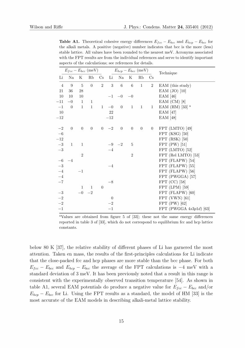
Appendix A. Lattice Stability

Owing to the history of lattice-stability calculations with various EAM formulations, we

include here a brief discussion of the relative stability of the bcc, fcc, and hcp lattices

for the five alkali metals. Using our potentials we have calculated the cohesive energy

for each lattice type; the cohesive energy differences Efcc − Ebcc and Ehcp − Ebcc are

reported in table A1. As indicated in the table, for all five alkali metals our potentials

predict the bcc lattice to be more stable than either the fcc or hcp lattices, with the

cohesive energy differences ranging from +0 to 9 meV. Insofar as our Efcc −Ebcc values

for Li, Na, and K all lie within the respective range of EAM-calculated values that have

been previously reported (also shown in table A1), our results are typical for an EAM

model.

It is informative to compare the EAM calculated results with those of first-principles

theory (FPT), which are also tabulated in table A1. Due to the transformation of Li

from the bcc phase to a close-packed configuration as the temperature is decreased

14


Table A1. Theoretical cohesive energy differences Efcc − Ebcc and Ehcp − Ebcc for

the alkali metals. A positive (negative) number indicates that bcc is the more (less)

stable lattice. All values have been rounded to the nearest meV. Acronyms associated

with the FPT results are from the individual references and serve to identify important

aspects of the calculations; see references for details.

Efcc − Ebcc (meV) Ehcp − Ebcc (meV)Technique

Li Na K Rb Cs Li Na K Rb Cs

4 9 5 0 2 3 6 6 1 2 EAM (this study)

21 36 28 EAM (JO) [10]

10 10 10 −1 −0 −0 EAM [46]

−11 −0 1 1 EAM (CM) [8]

−1 0 1 1 1 −0 0 1 1 1 EAM (HM) [33] a

10 22 EAM [47]

−12 −12 EAM [48]

−2 0 0 0 0 −2 0 0 0 0 FPT (LMTO) [49]

−6 FPT (KSG) [50]

−12 FPT (RSK) [50]

−3 1 1 −9 −2 5 FPT (PW) [51]

−3 −4 FPT (LMTO) [52]

2 2 FPT (Rel LMTO) [53]

−6 −4 FPT (FLAPW) [54]

−3 −4 FPT (FLAPW) [55]

−4 −1 FPT (FLAPW) [56]

−4 FPT (PWGGA) [57]

−7 −8 FPT (CC) [58]

1 1 0 FPT (LPM) [59]

−3 −0 −2 FPT (FLAPW) [60]

−2 0 FPT (VWN) [61]

−2 −2 FPT (PW) [62]

−1 −1 FPT (PWGGA 4s3p1d) [63]

aValues are obtained from figure 5 of [33]; these not the same energy differences

reported in table 3 of [33], which do not correspond to equilibrium fcc and hcp lattice

constants.

below 80 K [37], the relative stability of different phases of Li has garnered the most

attention. Taken en mass, the results of the first-principles calculations for Li indicate

that the close-packed fcc and hcp phases are more stable than the bcc phase. For both

Efcc − Ebcc and Ehcp − Ebcc the average of the FPT calculations is −4 meV with a

standard deviation of 3 meV. It has been previously noted that a result in this range is

consistent with the experimentally observed transition temperature [54]. As shown in

table A1, several EAM potentials do produce a negative value for Efcc − Ebcc and/or

Ehcp − Ebcc for Li. Using the FPT results as a standard, the model of HM [33] is the

most accurate of the EAM models in describing alkali-metal lattice stability.

15


References

[1] Daw M S and Baskes M I 1983 Phys. Rev. Lett. 50 1285

[2] Daw M S and Baskes M I 1984 Phys. Rev. B 29 6443

[3] Daw M S, Foiles S M and Baskes M I 1993 Materials Science Reports 9 251

[4] Nelson J S, Sowa E C and Daw M S 1988 Phys. Rev. Lett. 61 1977

[5] Nelson J S, Daw M S and Sowa E C 1989 Phys. Rev. B 40 1465

[6] Nelson J, Daw M and Sowa E C 1990 Superlattices and Microstructures 7 259

[7] Benedek G, Bernasconi M, Chis V, Chulkov E, Echenique P M, Hellsing B and Toennies J P 2010

J. Phys.: Condens. Matter 22 084020

[8] Chantasiriwan S and Milstein F 1998 Phys. Rev. B 58 5996

[9] Wang Y R and Boercker D B 1995 Journal of Applied Physics 78 122

[10] Johnson R A and Oh D J 1989 Journal of Materials Research 4 1195

[11] Johnson R A 1988 Phys. Rev. B 37 3924

[12] Guellil A M and Adams J B 1992 Journal of Materials Research 7 639

[13] Kittel C 2005 Introduction to Solid State Physics (New York: Wiley)

[14] MacDonald D K C 1953 The Journal of Chemical Physics 21 177

[15] Adlhart W, Fritsch G and Lscher E 1975 Journal of Physics and Chemistry of Solids 36 1405

[16] Mundy J N, Miller T E and Porte R J 1971 Phys. Rev. B 3(8) 2445

[17] Martin D L 1965 Phys. Rev. 139 A150

[18] Anderson M S and Swenson C A 1985 Phys. Rev. B 31 668

[19] Siegel S and Quimby S L 1938 Phys. Rev. 54 76

[20] Barrett C S 1956 Acta Crystallographica 9 671

[21] Schouten D R and Swenson C A 1974 Phys. Rev. B 10 2175

[22] Slotwinski T and Trivisonno J 1969 Journal of Physics and Chemistry of Solids 30 1276

[23] Quimby S L and Siegel S 1938 Phys. Rev. 54 293

[24] Martinson R H 1969 Phys. Rev. 178 902

[25] Marquardt W and Trivisonno J 1965 Journal of Physics and Chemistry of Solids 26 273

[26] Gutman E and Trivisonno J 1967 Journal of Physics and Chemistry of Solids 28 805

[27] Kollarits F and Trivisonno J 1968 Journal of Physics and Chemistry of Solids 29 2133

[28] Smith H G, Dolling G, Nicklow R M, Vijayaraghavan P R and Wilkinson M K 1968 Neutron

Inelastic Scattering 1 149

[29] Woods A D B, Brockhouse B N, March R H, Stewart A T and Bowers R 1962 Phys. Rev. 128

1112

[30] Cowley R A, Woods A D B and Dolling G 1966 Phys. Rev. 150 487

[31] Copley J R D and Brockhouse B N 1973 Canadian Journal of Physics 51 657

[32] Nucker N and Buchenau U 1985 Phys. Rev. B 31 5479

[33] Hu W and Masahiro F 2002 Modelling Simulation Mater. Sci. Eng. 10 707

[34] Zhang J M, Zhang X J and Xu K W 2008 Journal of Low Temperature Physics 150 730

[35] Xie Y and Zhang J M 2008 Canadian Journal of Physics 86 801

[36] Grimvall G 1981 The Electron-Phonon Interaction in Metals (New York: Oxford)

[37] Schwarz W, Blaschko O and Gorgas I 1991 Phys. Rev. B 44 6785

[38] Sklyadneva I Y, Chulkov E V and Bertsch A V 1996 Surface Science 352-354 25

[39] Sklyadneva I Y, Berch A V and Chulkov E V 1995 Phys. Solid State 37 1454

[40] Bohnen K P 1982 Surface Science 115 L96

[41] Bohnen K P 1984 Surface Science 147 304

[42] Rodach T, Bohnen K P and Ho K M 1989 Surface Science 209 481

[43] Quong A A, Maradudin A A, Wallis R F, Gaspar J A, Eguiluz A G and Alldredge G P 1991 Phys.

Rev. Lett. 66 743

[44] Andersson S, Pendry J and Echenique P 1977 Surface Science 65 539

[45] Wertheim G K, Riffe D M, Smith N V and Citrin P H 1992 Phys. Rev. B 46 1955

16


[46] Baskes M I 1992 Phys. Rev. B 46 2727

[47] Yuan X, Takahashi K, Yin Y and Onzawa T 2003 Modelling Simulation Mater. Sci. Eng. 11 447

[48] Cui Z, Gao F, Cui Z and Qu J 2012 Modelling Simulation Mater. Sci. Eng. 20 015014

[49] Skriver H L 1985 Phys. Rev. B 31 1909–1923

[50] Boettger J C and Trickey S B 1985 Phys. Rev. B 32 3391

[51] Dacorogna M M and Cohen M L 1986 Phys. Rev. B 34 4996

[52] Boettger J C and Albers R C 1989 Phys. Rev. B 39 3010

[53] Alouani M, Christensen N E and Syassen K 1989 Phys. Rev B 39 8096

[54] Sigalas M, Bacalis N C, Papaconstantopoulos D A, Mehl M J and Switendick A C 1990 Phys. Rev.

B 42 11637

[55] Nobel J A, Trickey S B, Blaha P and Schwarz K 1992 Phys. Rev. B 45 5012

[56] Papaconstantopoulos D A and Singh D J 1992 Phys. Rev. B 45 7507

[57] Perdew J P, Chevary J A, Vosko S H, Jackson K A, Pederson M R, Singh D J and Fiolhais C 1992

Phys. Rev. B 46 6671

[58] Cho J H, Ihm S H and Kang M H 1993 Phys. Rev. B 47 14020

[59] Mutlu R H 1995 Phys. Rev. B 52 1441

[60] Sliwko V L, Mohn P, Schwarz K and Blaha P 1996 J. Phys.: Condens. Matter 8 799

[61] Staikov P, Kara A and Rahman T S 1997 J. Phys.: Condens. Matter 9 2135

[62] Liu A Y, Quong A A, Freericks J K, Nicol E J and Jones E C 1999 Phys. Rev. B 59 4028

[63] Doll K, Harrison N M and Saunders V R 1999 Journal of Physics: Condensed Matter 11 5007

17

Documents

An Embedded-Atom-Method Model for Alkali-Metal Vibrations Alkali Vibrations IOP.pdf · An Embedded-Atom-Method Model for Alkali-Metal Vibrations R B Wilson and D M Ri e ... Abstract