HAL Id: hal-00851429https://hal.inria.fr/hal-00851429

Preprint submitted on 14 Aug 2013

HAL is a multi-disciplinary open accessarchive for the deposit and dissemination of sci-entific research documents, whether they are pub-lished or not. The documents may come fromteaching and research institutions in France orabroad, or from public or private research centers.

L’archive ouverte pluridisciplinaire HAL, estdestinée au dépôt et à la diffusion de documentsscientifiques de niveau recherche, publiés ou non,émanant des établissements d’enseignement et derecherche français ou étrangers, des laboratoirespublics ou privés.

An empirical analysis of heavy-tails behavior of financialdata: The case for power laws

Nicolas Champagnat, Madalina Deaconu, Antoine Lejay, Nicolas Navet,Souhail Boukherouaa

To cite this version:Nicolas Champagnat, Madalina Deaconu, Antoine Lejay, Nicolas Navet, Souhail Boukherouaa. Anempirical analysis of heavy-tails behavior of financial data: The case for power laws. 2013. �hal-00851429�

An empirical analysis of heavy-tails behaviorof financial data: The case for power laws

Nicolas Champagnatb,c,d,† Madalina Deaconub,c,d,†

Antoine Lejayb,c,d,† Nicolas Navete,‡ Souhail Boukherouaaa,b,c,d

August 14, 2013

Abstract

This article aims at underlying the importance of a correct modelling of theheavy-tail behavior of extreme values of financial data for an accurate risk estima-tion. Many financial models assume that prices follow normal distributions. This isnot true for real market data, as stock (log-)returns show heavy-tails. In order toovercome this, price variations can be modeled using stable distribution, but then,as shown in this study, we observe that it over-estimates the Value-at-Risk. To over-come these empirical inconsistencies for normal or stable distributions, we analyzethe tail behavior of price variations and show further evidence that power-law distri-butions are to be considered in risk models. Indeed, the efficiency of power-law riskmodels is proved by comprehensive backtesting experiments on the Value-at-Riskconducted on NYSE Euronext Paris stocks over the period 2001-2011.

Keywords: model for log-returns of assets; Value-at-Risk; risk management; power taildistribution; stable distribution; normal distribution; Hill estimator; backtesting.

AMS classification (2010): 62G32

JEL classification: C14, C18, G11

1 IntroductionThe Value-at-Risk (VaR) is one of the main indicators for risk management of financialportfolios [47]. It is expressed as the threshold that a loss over a chosen time horizonoccurs with at most a given level of confidence.

The VaR may be estimated either by parametric or non-parametric approach. Thenon-parametric one uses only the empirical distributions (historical, resampling) withoutaAlphability, F-54500 Vandoeuvre-lès-Nancy, France.b Université de Lorraine, Institut Elie Cartan de Lorraine, UMR 7502, Vandoeuvre-lès-Nancy, F-54506,

France.c CNRS, Institut Elie Cartan de Lorraine, UMR 7502, Vandoeuvre-lès-Nancy, F-54506, France.d Inria, Villers-lès-Nancy, F-54600, France.e FSTC/CSC Research Unit/Lassy lab., Université du Luxembourg, L-1359 Luxembourg.† Email: {Nicolas.Champagnat,Madalina.Deaconu,Antoine.Lejay}@inria.fr‡ Email: nicolas.navet@uni.lu

1

fitting a model. Due to the small amount of available data, it does not provide an accurateway to deal with extreme events. On the other hand, the parametric approach consistsin fitting the parameters of a model on historical data and compute afterwards the VaR,either by analytic or numerical methods.

The RiskMetric methodology [64] is widely used to estimate the risk associated to aPortfolio through the computations relating variations of the risk indicator to variationsof risk factors (stocks and prices derivatives for example). Nowadays this methodology in-corporates heavy tail distributions, but it was initially developed in the Gaussian context,which is still prevalent is risk management and enforced by Basel Accord [77].

However, actual regulations and standard ways of computing the VaR, mainly relatedto the Gaussian world, have been invalidated by studies (see e.g. [2, 7]) because theyseverely underestimate the risk observed in the market.

The successive financial crisis since 1987 have led to a greater attention to tail behaviorof the induced (log-)returns distributions, and using Extreme Value Theory (EVT) hasbeen pushed forward as a central concept in Risk Management (See e.g. [13, 24]).

Using a model for the tail distributions overrides partially the problem induced by thelack of data for computing the VaR with historical distributions. Once a model for the(log-)returns is specified and calibrated, the VaR, as it is related to the quantiles of thedistribution, can be computed through tractable expressions or simulations. Other riskindicators as the CVaR or expected shortfall may be computed as well.

There is no single model nor statistical methodology which are acknowledged as stan-dard for dealing with heavy-tails. In this study, we choose to stick on the simplest possiblemodels. Calibrating a complex model leads to high uncertainties on the parameters whichdecreases its intricate qualities for practical use, especially with small data samples.

Let us point that we focus here only on univariate distributions. The case of severalassets leads to higher complexity, as the notion of VaR itself should be properly defined(See e.g. [73]). The multivariate case will be subject to further studies.

As the Gaussian models underestimate extreme losses, we consider heavy tails distri-butions for the log-returns 𝐿 with distribution function 𝐹 , typically, generalized Pareto(power laws):

1 − 𝐹 (𝑥) = P[𝐿 ≥ 𝑥] =ℓ(𝑥)

𝑥𝛼for 𝑥 ≥ 𝑥0, (1)

where ℓ is a function of regular variation, 𝛼 is the tail index and 𝑥0 is a threshold abovewhich the power law holds. This formula deals only with the tail distribution. We givein Section 2 a literature review of heavy-tailed models, together with empirical evidencesof their relevance in finance and estimation procedures.

This work aims at studying the performance of VaR estimators for three classes ofmodels (Gaussian, stable and Pareto tails) on historical market data from NYSE EuronextParis. We focus only on daily log-returns of single stock prices.

Outline. In Section 2, we give an overview of models with heavy-tails used in finance,the markets on which they have been applied and the estimators for power laws. InSection 3, we introduce our methodology for estimating the parameters and performingthe backtesting. Finally, in Section 4, we present our dataset as well as the conclusionswe drawn from the study over a selection of 71 assets from NYSE Euronext Paris. Someperspectives and conclusions are then presented in Section 5.

2

2 Overview of heavy tails: models, empirical evidences and esti-mations

2.1 Some commonly used models for heavy tails

Normal distributions and Brownian motion in finance go back to Bachelier’s thesis [5] andwere popularized by F. Black and M. Scholes in the 70’s [8].

There are several reasons making log-normal returns appealing. The first one is thatthey could be simply interpreted and estimated. Second, closed-form expression existsfor several options. Third, they could be embedded in a continuous time process, as thegeometric Brownian motion, which models the evolution of the stock over the time.

Indeed, many theories, for example the Capital Asset Pricing Model (CAPM) forportfolio management [61], take their roots in the Gaussian world.

However, starting with B. Mandelbrot [59] in the 60’s, it has been evidenced thatnormal or log-normal distributions do not fit some of the stylized facts, mainly in regardto skewness and heavy tail of observed distributions.

A large amount of literature in quantitative finance deals with the problem of findingtractable models which reproduce heavy-tails returns or log-returns.

Stable distributions and processes have been proposed first by B. Mandelbrot [59] andE.F. Fama [30]. This popular approach is referred to as the “Paretian world”. As forthe Gaussian world, the log-returns of a given stock may be embedded in a stochasticdiscontinuous process while having a heavy-tail decreasing like a power law of index 𝛼.The CAPM can also be extended in some directions. Yet choosing this model imposesthat 𝛼 < 2. This parameter is however difficult to estimate, especially when close to 2[27]. In addition to the references and empirical studies cited above, which backed that𝛼 may be greater than 2, let us cite [9, 12, 49] as containing critics on the stable model.

Thus, many alternatives have been sought. There is a huge literature on this sub-ject [71], so that we give the main lines with a focus only on univariate returns. Regardingstochastic processes in continuous time, let us cite jump diffusion models [19, 50], vari-ance Gamma processes [60] and subordinated processes [16], and SDE whose invariantdistributions are fat-tailed [67, 74] or present moments explosions [38, Chapter 7].

Along with continuous time stochastic processes, chronological series play a very im-portant role in the development of such financial models for stock prices. The (log-)returnsare solutions to equations of the form 𝑟𝑡+1 = 𝜇𝑟𝑡 + 𝜎𝑡𝜖𝑡, where 𝜎𝑡 is itself described by anequation of similar form. One of the most popular model is the General AutoregressiveConditional Heteroskedasticity (GARCH) model which captures clustering effects. Here,the innovation 𝜖𝑡 is a noise, that could be Gaussian or follow a given distribution. Amongthem, Student’s 𝑡 distributions have been widely studied. We refer for example to [21, 52]and their introduction to references in this field. In [76], A.K. Singh et al. give a specificaccount on such model in relation with power laws.

Finally, another approach consists in separating the tail of the distribution from itsbulk through hybrid models. Several approaches may be found in [72]. Furthermore,mixtures of models may also lead to heavy tails [14].

2.2 Evidences for the power law in financial markets

It is widely acknowledged that prices and returns of assets obey to general laws usu-ally called “stylized facts” [17]. Skewness and heavy-tail are the two main properties ofobserved prices which are not verified by the Black & Scholes models.

Although stable distributions have been proposed since the 60’s [30, 59] and an alter-

3

native model (finite variance subordinated log-normal distributions) has been proposedin 1973 by P. Clark [16], the systematic use of Extreme Value Theory (EVT) is morerecent, as the crash of 1987 urged for a better understanding of large losses. For the firstoccurrences of the use of EVT focusing only on the tail distributions, let us cite [43, 54,56].

Soon, the availability of large datasets and the failure of normal distributions to repli-cate the extreme movements led to a blossoming of empirical studies about EVT.

Of course, crises such as the Asian crisis, have been subjects of particular impor-tance [41, 48]. Another body of works concerns emerging markets: Asia [36, 48], MENAregion [4], Turkey [36, 78], Latin America [36, 44], ...

Developed markets have been investigated as well, mainly through market indices:S&P 500, Dow Jones and Nasdaq [37, 54, 57, 58, 76], German DAX Stocks [25], AustralianASX-ALL [76], Nikkei and Eurostoxx 50 [37], ...

Finally, the EVT has also been applied to other prices, such as exchanges rates (Seee.g. [45, 49]), futures margins [20], ...

In all these situations, the normal hypotheses is rejected as a model for the returndistributions and heavy tails should be taken into account. However, the stable hypothesisseems too strong.

In many situations, it is recorded that the variance of the returns is finite [4, 36, 37,48] and the tail index lies between 2 and 5. Some authors note that regarding extremeevents, markets in emerging and developed countries present similar features [48]. In [35],X. Gabaix summarizes various studies on power law in finance and defend the notion of“universality” of a tail index around 3 for short terms returns.

In addition, to these empirical evidences, a growing body of literature also focuses oneconomic and agent based models which could explain fat tails and phenomena leadingto them, such as volatility clustering. This subject is beyond the scope of this article andwe refer for example only to [18, 33] and related references therein.

2.3 Estimators for the tail index

The tail index 𝛼 summarizes the heaviness of the tail distributions, and characterizes alsothe existence of moments. Hence, let us consider that the (log-)return 𝑋 at a given timesatisfies (1) and that 𝑛 successive (log-)returns (𝑋1, . . . , 𝑋𝑛) are independent or at leaststationary.

It is a crucial and complex problem to estimate 𝛼 and ℓ(𝑥) written in a parametric orsemi-parametric form (for example, ℓ(𝑥) = 𝐶 or ℓ(𝑥) = 𝐶1+𝐶2/𝑥

𝛽+o(𝑥−𝛽)), as well as 𝑥0.For studying the tail of the distribution of 𝑋, we use the order statistics (𝑋(1), . . . , 𝑋(𝑛))of (𝑋1, . . . , 𝑋𝑛) with 𝑋(1) ≤ 𝑋(2) ≤ · · · ≤ 𝑋(𝑛).

Estimating 𝛼 is a difficult problem in general due to the lack of observed extremeevents, by their very definition.

The literature is too wide to be cited here. Estimators may in general be attached toone of the following families, none of them superseding the others:∙ Hill type estimator. The Hill estimator [40] provides us with

𝐻𝑘,𝑛 = 𝑘−1

𝑘∑

𝑗=1

ln𝑋(𝑛−𝑗+1) − ln𝑋(𝑛−𝑘)

as an estimator of 𝛾 = 1/𝛼. There are several ways to interpret this estimator (maximumlikelihood, least squares, ...). The main difficulty for its implementation consists in choos-ing the optimal index 𝑘, which gave rise to a huge literature. A large part of it consists

4

in assuming that ℓ(𝑥) is not constant and balancing between the Monte Carlo error andthe bias. Generalizations of Hill estimator include least-square estimators. See e.g. [42]for an application to financial data. On the Hill estimator and its variants, we refer tothe book [6] and references therein.The Hill method gave rise to a graphical procedure, the Hill Plot [26], which consists inplotting (𝑘,𝐻𝑘,𝑛). The lack of stability of the produced graph leads to a lot of critics, theHill Plot being dubbed as the “Hill horror plot”.∙ The Pickands estimator [70], estimates 𝛼 = 1/𝛾 from a slope using three points.

Again, a tail index 𝑘 should be carefully chosen.∙ The Peak over Threshold (POT) method [29], is popular in the hydrogeology commu-

nity and also led to a graphical procedure. It relies on the convergence of the distributionfunction of the renormalized maximum of the data toward a Generalized Extreme Valuedistribution. Applications to financial market may be found in [3, 37].∙ Block maxima, which consists in focusing on the statistics of the maxima of blocks of

data in link with their frequency (See e.g. [31] and references within).∙ Other estimators: many variants of the Hill and Pickands estimators have been pro-

posed, using for example the moments [22] or the median of the order statistics, the DRPestimator [69], ...

Finally, several methods have been proposed to deal specifically with the four pa-rameters of stable distributions: quantile estimation [63], maximum likelihood [28, 65],characteristic functions [32, 51]. See also [27, 62, 80] for critical reviews.

3 Framework and methodology3.1 Log returns and Value-at-Risk

Let us consider the prices of a financial asset (𝑆𝑡, 𝑡 ≥ 0) where time is measured on daysunits. We define the daily log-returns as being the sequence (𝑅𝑡, 𝑡 ∈ N) given by

𝑅𝑡 = ln

(𝑆𝑡+1

𝑆𝑡

)= ln(𝑆𝑡+1) − ln(𝑆𝑡). (2)

We call also log-losses the values 𝐿𝑡 = −𝑅𝑡 for 𝑅𝑡 < 0.The statistical principle of risk estimation consists in assuming that the 𝑅𝑡’s are inde-

pendent realizations of a given law.The Value-at-Risk (VaR) at a level 𝛼 ∈ (0, 1), and for the horizon 𝑇 = 1 (one day), of

a financial asset (𝑆𝑡, 𝑡 ≥ 0), is the lowest amount not exceeded by the loss with probability𝛼 (usually 𝛼 is close to 1), i.e.

1 − 𝛼 = P (𝑆1 − 𝑆0 < −VaR𝛼) . (3)

In this article, we consider only daily VaR. The 1-day VaR𝛼 may be expressed by thedaily log-returns as follows: for 𝛼 close to 1,

1 − 𝛼 = P(𝑅1 < 𝑞𝑅1−𝛼) with VaR𝛼 = 𝑆0(1 − exp(𝑞𝑅1−𝛼)) (4)

or1 − 𝛼 = P(𝐿1 > 𝑞𝐿𝛼) with VaR𝛼 = 𝑆0(1 − exp(−𝑞𝐿𝛼)), (5)

where 𝑞𝑋𝛼 is the 𝛼-quantile of the random variable 𝑋.After having chosen a class of parametric models, the practical computation of the

VaR consists in calibrating the parameters for the common distribution of 𝑅 or 𝐿 of dailylog-returns or log-losses and computing the quantile 𝑞𝑅1−𝛼 or 𝑞𝐿𝛼 . We need to know onlythe tail of the distribution.

5

3.2 Models

We consider three classes of parametric univariate models for the log-returns or log-losses:(I) The classical Gaussian family for the log-returns defined by its mean 𝜇 and

standard deviation 𝜎.(II) The stable distribution for the log-returns defined by its characteristic function

𝜑𝑋(𝑡) =

{exp[𝑖𝜇𝑡− 𝜎𝛼|𝑡|𝛼(1 − 𝑖𝛽 sign(𝑡) tan(𝜋𝛼

2))] if 𝛼 = 1

exp[𝑖𝜇𝑡− 𝜎|𝑡|(1 + 2𝜋𝑖𝛽 sign(𝑡) ln |𝑡|)] if 𝛼 = 1,

(6)

where 𝛼 ∈ (0, 2) is the tail index, 𝛽 ∈ (−1, 1) is the skewness, 𝜎 ≥ 0 is the scale parameterand 𝜇 ∈ R the location parameter (See e.g. [34, 68]).(III) The Pareto distribution for tails of the log-losses gives for the distributionfunction 𝐹 of the log-losses,

P[𝐿𝑡 > 𝑥] = 1 − 𝐹 (𝑥) = 𝐶/𝑥𝛼 for 𝑥 ≥ 𝑥0. (7)

This model does not make any supplementary assumption on the bulk of the distributionof the log-returns.

Gaussian distributions are a particular case of stable distributions for 𝛼 = 2. However,in this case, 𝛼 does not correspond to the tail index. When 𝛼 < 2, a stable distributionis in fact a Generalized Pareto distribution with

P[𝑋 ≤ 𝑥] ≈ 𝐶st

|𝑥|𝛼 when 𝑥 → −∞ with 𝐶st = 𝜎𝛼 sin(𝜋𝛼

2

) Γ(𝛼)

𝜋(1 − 𝛽), (8)

where Γ denotes the Gamma function [68, Theorem 1.12].Gaussian and stable distributions arise naturally as universal classes when looking to

limit theorems. The micro-economic justification assumes that the prices are fixed by theinteractions of a large amounts of small independent prices changes. Stable distributionsare fat-tailed. Yet they have an infinite variance which sometimes produces too highextremes events with respect to the observed log-returns (See Section 2).

Pareto distributions offer a wider variety of fat tails by removing the constraint 𝛼 < 2.

3.3 Parameters estimation and computation of the VaR

Before describing the methods we used to estimate the parameters of the chosen distribu-tions and then to compute the quantiles, we should make the following remark: Choosinga model requires that the series of stock prices (𝑆𝑡) is stationary over the time. This isof course not true for prices spanning over several years. Thus, we apply our estimatorsover a finite window of time, 1 year in our experiments, where the prices are assumed tobe stationary.

(I) Gaussian distribution Considering 𝑛 successive daily log-returns (𝑅1, . . . , 𝑅𝑛)assumed to follow the Gaussian distribution of mean 𝜇 and standard deviation 𝜎, we set

�� =1

𝑛

𝑛∑

𝑖=1

𝑅𝑖, and �� =

(1

𝑛− 1

𝑛∑

𝑖=1

(𝑅𝑖 − ��)2

)1/2

,

and the (1− 𝛼)-quantile 𝑞𝑅1−𝛼 is approximated by 𝑞𝑅1−𝛼 = ��+ Φ−1(1− 𝛼)�� where Φ is thestandard Gaussian distribution function.

6

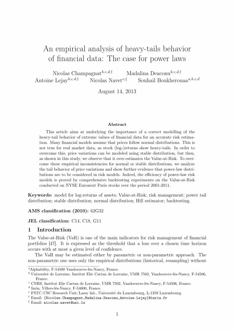
(II) Stable Distribution For the stable distribution, we use for the log-returns the Mc-Culloch method as implemented in the R library fBasics to estimate the four parameters𝛼, 𝛽, 𝜎 and 𝜇 and to compute the quantile through a direct estimation of the distributionfunction.(III) Pareto distribution We use a slight modification of the Hill estimator. Let(𝐿(1), . . . , 𝐿(𝑛)) be the increasing order statistics of 𝑛 independent log-losses (𝐿1, . . . , 𝐿𝑛)whose common distribution is assumed to satisfy P[𝐿1 ≥ 𝑥] = 𝐶/𝑥𝛼 for 𝑥 ≥ 𝑥0.For 𝑖 large enough,

ln𝐿(𝑖) = −𝛾 ln

(𝑛 + 1 − 𝑖

𝑛 + 1

)+ 𝐾 + 𝜀𝑖, (9)

where 𝛾 = 1/𝛼, 𝐾 = 𝛾 ln𝐶 is a constant and 𝜀𝑖 is a noise. Plotting ln𝐿(𝑖) as a functionof − ln((𝑛+ 1− 𝑖)/(𝑛+ 1)) gives a Pareto plot. The Hill estimator allows to compute theslope of such a graph, using a weighted least squares estimation. For more stability, weuse a variant of this estimator by removing the highest values. After fixing an interval[𝑑𝑛, 𝑢𝑛], an estimator 𝛾 of 𝛾 = 𝛼−1 is given by a standard least squares procedure on (9)for 𝑖 ∈ [𝑑𝑛, 𝑢𝑛]:

𝛾 = −∑𝑢𝑛

𝑖=𝑑𝑛ln(𝐿(𝑖)) · ln

(𝑛+1−𝑖𝑛+1

)∑𝑢𝑛

𝑖=𝑑𝑛

(ln(𝑛+1−𝑖𝑛+1

))2 .

The constant 𝐶 in (7) could be estimated as well by exp(����) where �� = 1/𝛾 and ��is given by the least square procedure on (9). However, we choose a procedure which isnumerically more stable by borrowing ideas from I. Weissman [79]. For 𝑤 ∈ (0, 1) closeto 1, the constant 𝐶 and the threshold 𝑥0 in (7) are estimated by

𝐶 = 𝐿��⌊𝑛𝑤⌋(1 − 𝑤) and ��0 = 𝐿⌊𝑛𝑤⌋. (10)

The rationale of this approximation is that 𝐿⌊𝑛𝑤⌋ is an approximation of the quantile 𝑞𝑤of (𝐿1, . . . , 𝐿𝑛). The quantile of the log-losses at level 𝑝 ≥ 𝑤 is then approximated by

𝑞𝐿𝑝 =

(𝐶

1 − 𝑝

)𝛾

= 𝐿⌊𝑛𝑤⌋

(1 − 𝑤

1 − 𝑝

)𝛾

.

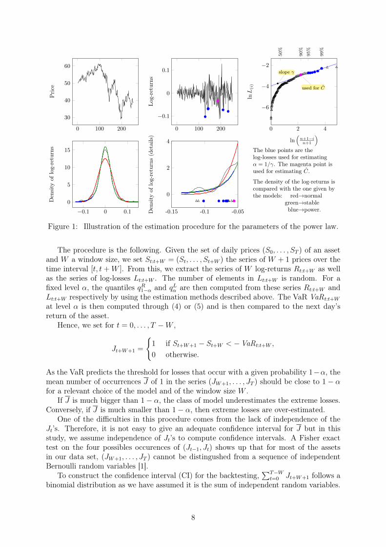
This procedure is illustrated over one year (252 data) of real data in Fig. 1. The firsttwo figures represents the evolution of the prices and the log-returns. The third plot isthe Pareto plot, where the points used for the statistical estimation of 𝛾 are marked inblue, while the one used for the estimation of 𝐶 is marked in magenta. The last two plotsrepresent the empirical densities of the log-returns, with a zoom on the large losses, as wellas the fitted models for normal (red), stable (green) and power tail (blue) distributions.

3.4 Choice of the parameters of the tail index estimator

We estimated the power law distribution by setting 𝑑𝑛 = ⌊0.95×𝑛⌋, 𝑢𝑛 = ⌊0.99×𝑛⌋ and𝑤 = 0.90, where 𝑛 is the number of log-losses.

As the window size is 𝑊 = 252, it has been observed on all the assets that the numberof log-losses is around 𝑊/2. This means that the parameters for extreme log-losses areestimated from very small samples.

3.5 Backtesting

The backtesting procedure consists in comparing the estimated VaR with the real numberof extreme losses [15].

7

0 100 200

30

40

50

60

Pri

ce

0 100 200

−0.1

0

0.1

Log-

retu

rns

0 2 4

−6

−4

−2slope γ

used for C

ln(

n+1−in+1

)

lnL(i)

50%

90%

95%

99%

−0.1 0 0.1

0

5

10

15

Den

sity

oflo

g-re

turn

s

-0.15 -0.1 -0.05

0

2

4

Den

sity

oflo

g-re

turn

s(d

etai

ls)

The blue points are thelog-losses used for estimatingα = 1/γ. The magenta point isused for estimating C.

The density of the log-returns iscompared with the one given bythe models: red→normal

green→stableblue→power.

Figure 1: Illustration of the estimation procedure for the parameters of the power law.

The procedure is the following. Given the set of daily prices (𝑆0, . . . , 𝑆𝑇 ) of an assetand 𝑊 a window size, we set 𝑆𝑡:𝑡+𝑊 = (𝑆𝑡, . . . , 𝑆𝑡+𝑊 ) the series of 𝑊 + 1 prices over thetime interval [𝑡, 𝑡 + 𝑊 ]. From this, we extract the series of 𝑊 log-returns 𝑅𝑡:𝑡+𝑊 as wellas the series of log-losses 𝐿𝑡:𝑡+𝑊 . The number of elements in 𝐿𝑡:𝑡+𝑊 is random. For afixed level 𝛼, the quantiles 𝑞𝑅1−𝛼 and 𝑞𝐿𝛼 are then computed from these series 𝑅𝑡:𝑡+𝑊 and𝐿𝑡:𝑡+𝑊 respectively by using the estimation methods described above. The VaR VaR𝑡:𝑡+𝑊

at level 𝛼 is then computed through (4) or (5) and is then compared to the next day’sreturn of the asset.

Hence, we set for 𝑡 = 0, . . . , 𝑇 −𝑊 ,

𝐽𝑡+𝑊+1 =

{1 if 𝑆𝑡+𝑊+1 − 𝑆𝑡+𝑊 < −VaR𝑡:𝑡+𝑊 ,

0 otherwise.

As the VaR predicts the threshold for losses that occur with a given probability 1−𝛼, themean number of occurrences 𝐽 of 1 in the series (𝐽𝑊+1, . . . , 𝐽𝑇 ) should be close to 1 − 𝛼for a relevant choice of the model and of the window size 𝑊 .

If 𝐽 is much bigger than 1 − 𝛼, the class of model underestimates the extreme losses.Conversely, if 𝐽 is much smaller than 1 − 𝛼, then extreme losses are over-estimated.

One of the difficulties in this procedure comes from the lack of independence of the𝐽𝑡’s. Therefore, it is not easy to give an adequate confidence interval for 𝐽 but in thisstudy, we assume independence of 𝐽𝑡’s to compute confidence intervals. A Fisher exacttest on the four possibles occurences of (𝐽𝑡−1, 𝐽𝑡) shows up that for most of the assetsin our data set, (𝐽𝑊+1, . . . , 𝐽𝑇 ) cannot be distingushed from a sequence of independentBernoulli random variables [1].

To construct the confidence interval (CI) for the backtesting,∑𝑇−𝑊

𝑡=0 𝐽𝑡+𝑊+1 follows abinomial distribution as we have assumed it is the sum of independent random variables.

8

An exact CI at 100 × (1 − 𝜅)% is given by[

1

1 + 𝑛−𝑘+1𝑘

𝐹2(𝑛−𝑘+1),2𝑘(1 − 𝜅/2),

𝑘+1𝑛−𝑘

𝐹2(𝑘+1),2(𝑛−𝑘)(1 − 𝜅/2)

1 + 𝑘+1𝑛−𝑘

𝐹2(𝑘+1),2(𝑛−𝑘)(1 − 𝜅/2)

],

where 𝑘 is the number of successes, 𝑛 is the size of the sample, and 𝐹𝜈1,𝜈2(𝑝) is the inverseof the quantile at level 𝑝 ∈ [0, 1] of the 𝐹 -distribution with degree of freedoms 𝜈1 and 𝜈2[10, 11, 66].

4 Discussion: Empirical results and backtesting analysis4.1 The dataset: stocks from Euronext Paris

The financial instruments considered in the experiments are stocks exchanged on NYSEEuronext Paris. The market data are provided by eSignal (Interactive Data), and, inthe following, the stocks are identified by their eSignal symbol. Out of all the stockslisted on the Euronext Paris exchange in February 2011, more than 600, we selected oneshaving quotations throughout all the period ranging from January 2001 till February2011 (more than 11 years). This leads us with a subset of 71 stocks including some ofthe most liquid stocks making up the CAC40 index. In the following experiments, thetime series considered are the log-returns of the end-of-day closing prices of the selectedstocks and the parameters of the returns distributions are estimated on a sample madeof the last 252 last prices (walk-forward parameter setting). This window length set toone year is a trade-off between the need to have enough data to include recent crises andthe increased risk of departure from the stationarity hypothesis with larger data sets.Regarding the stationarity, it is difficult to draw a clear cut conclusion from Dickey-Fullerand Kwiatkowski–Phillips–Schmidt–Shin tests on unit root and stationarity tests [23, 53].We were not able in our experiments to identify other sample sizes that would consistentlyoutperform one year with regard to the VaR backtesting or stationarity measures.

4.2 Discussion

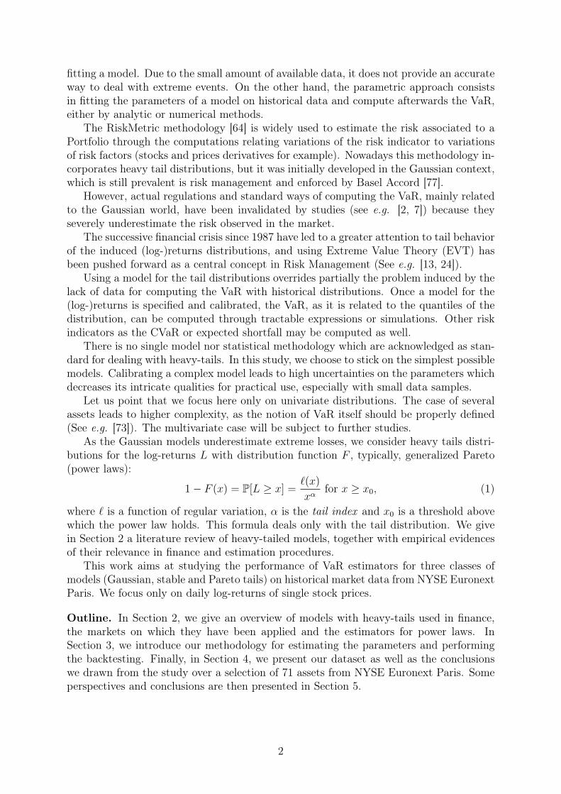
We applied the methods of estimation of the Value-at-Risk and of backtesting describedin Section 3 on the data described above. We plotted for all the assets the asset prices,the historical volatility computed from one-year data over a moving window, and theVaR computed with our three methods (Gaussian, stable and power law) from one yeardata over a moving window. We then selected 71 assets which sampled all the qualitativebehaviors that we could observe in the curves. The list of these assets is found on thehorizontal axis of Fig. 2.

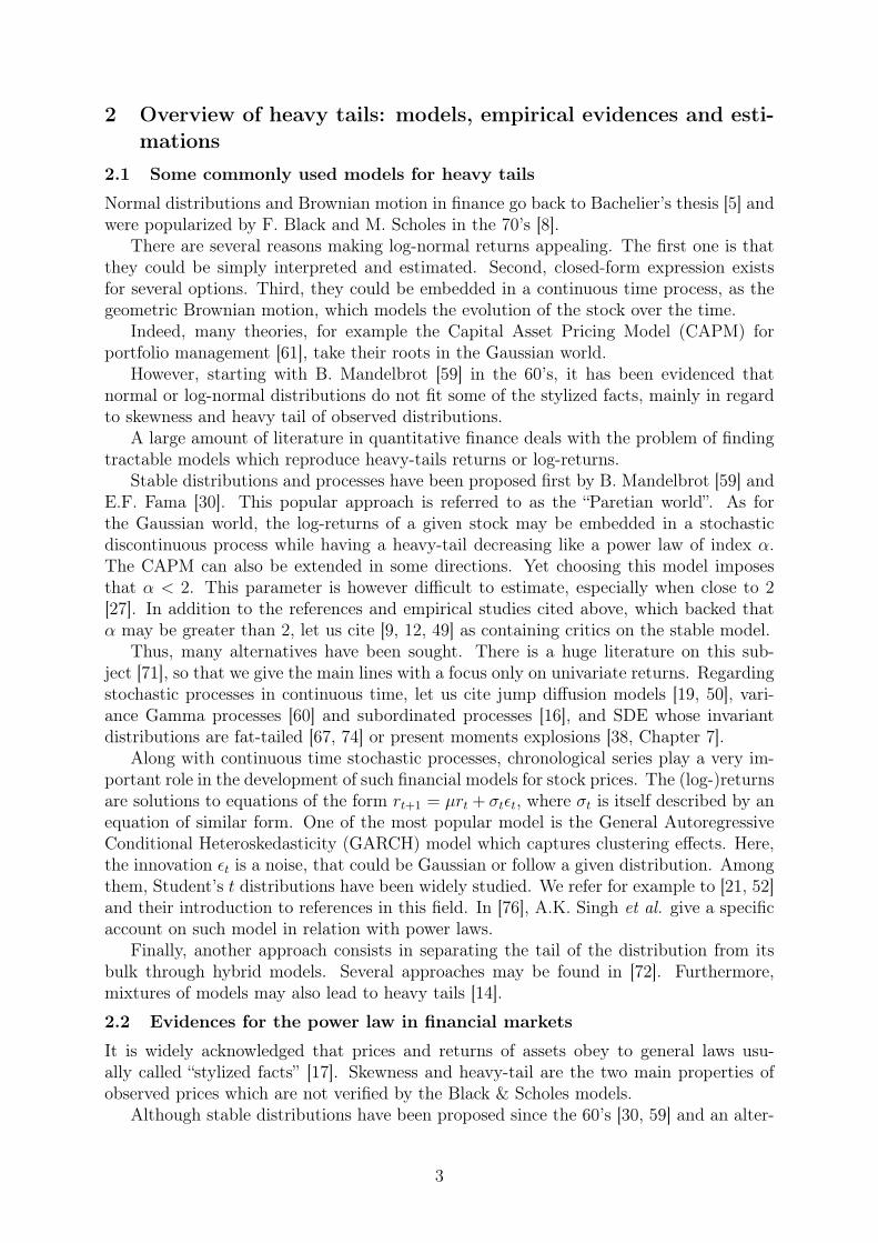
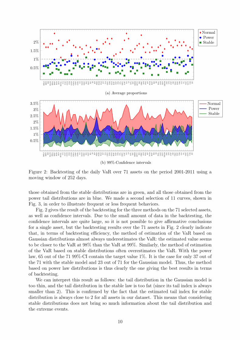
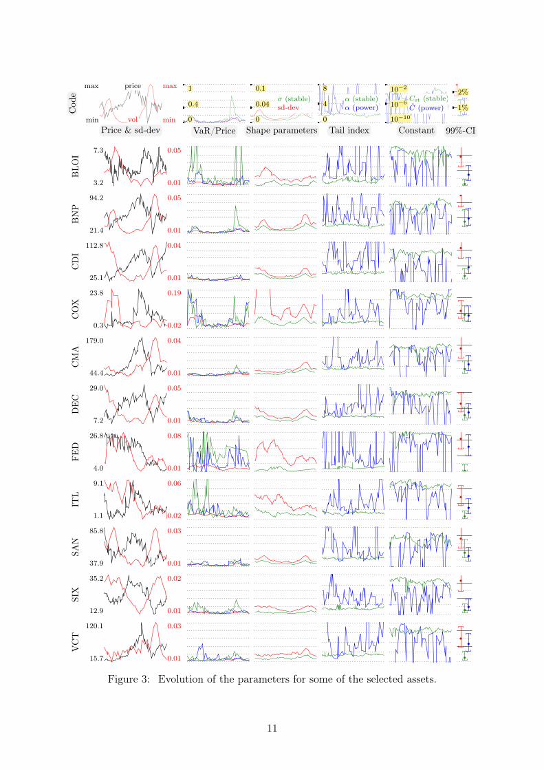
For all these 71 assets, we plotted 5 pictures as in Fig. 3, representing:(a) The asset price and volatility.(b) The relative VaR, that is the ratio of the VaR and the price, computed with our

three methods.(c) The volatility and the estimated value of the parameter 𝜎 of the stable distributions.(d) The estimated value of the tail index 𝛼 for the stable and power tail distributions.(e) At logarithmic scale, the estimated value of the constant 𝐶 of the tail distribution

of the stable distribution or power tail distribution, given in (8) and (10).(f) The 99%-CI for each of the models.

All these curves are computed over a one year moving window of data, and representedas a function of the last day of the moving window. We used the following color code: allthe curves obtained from an estimation based on the Gaussian distribution are in red, all

9

beli

ben bh

bloi

bna

bnp

bsd

bui

bull ca cas

ccn

cdi

cgd

cma

cnp

cox cs

dan

dec dg

dlt ec ei en fed

fgr

fle fp ga

gfc gid

gle

hav igf

ite

itl

key laf

lg lilv

lmc

mrb

mtu nk

orc osi

pig pp

pub

rcf

re ri

rll

san

sdt

sech six

spi

stf

sw tec

tff

tri

ug ul

vac

vct

vie zc

0.5%

1%

1.5%

2%

NormalPowerStable

(a) Average proportions

beli

ben bh

bloi

bna

bnp

bsd

bui

bull ca cas

ccn

cdi

cgd

cma

cnp

cox cs

dan

dec dg

dlt ec ei en fed

fgr

fle fp ga

gfc gid

gle

hav igf

ite

itl

key laf

lg lilv

lmc

mrb

mtu nk

orc osi

pig pp

pub

rcf

re ri

rll

san

sdt

sech six

spi

stf

sw tec

tff

tri

ug ul

vac

vct

vie zc

0.5%

1%

1.5%

2%

2.5%

3%

3.5% NormalPowerStable

(b) 99%-Confidence intervals

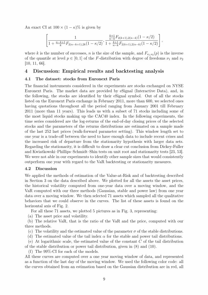
Figure 2: Backtesting of the daily VaR over 71 assets on the period 2001-2011 using amoving window of 252 days.

those obtained from the stable distributions are in green, and all those obtained from thepower tail distributions are in blue. We made a second selection of 11 curves, shown inFig. 3, in order to illustrate frequent or less frequent behaviors.

Fig. 2 gives the result of the backtesting for the three methods on the 71 selected assets,as well as confidence intervals. Due to the small amount of data in the backtesting, theconfidence intervals are quite large, so it is not possible to give affirmative conclusionsfor a single asset, but the backtesting results over the 71 assets in Fig. 2 clearly indicatethat, in terms of backtesting efficiency, the method of estimation of the VaR based onGaussian distributions almost always underestimates the VaR: the estimated value seemsto be closer to the VaR at 98% than the VaR at 99%. Similarly, the method of estimationof the VaR based on stable distributions often overestimates the VaR. With the powerlaw, 65 out of the 71 99%-CI contain the target value 1%. It is the case for only 37 out ofthe 71 with the stable model and 23 out of 71 for the Gaussian model. Thus, the methodbased on power law distributions is thus clearly the one giving the best results in termsof backtesting.

We can interpret this result as follows: the tail distribution in the Gaussian model istoo thin, and the tail distribution in the stable law is too fat (since its tail index is alwayssmaller than 2). This is confirmed by the fact that the estimated tail index for stabledistribution is always close to 2 for all assets in our dataset. This means that consideringstable distributions does not bring so much information about the tail distribution andthe extreme events.

10

max

min

max

min

price

vol

Cod

e

Price & sd-dev0

1

0.4

VaR/Price0

0.1

0.04σ (stable)sd-dev

Shape parameters0

8

4α (stable)α (power)

Tail index10−10

10−2

10−6Cst (stable)C (power)

Constant

1%

2%

99%-CI

7.3

3.2

0.05

0.01

BLO

I

94.2

21.4

0.05

0.01

BN

P

112.8

25.1

0.04

0.01

CD

I

23.8

0.3

0.19

0.02

CO

X

179.0

44.4

0.04

0.01

CM

A

29.0

7.2

0.05

0.01

DE

C

26.8

4.0

0.08

0.01

FE

D

9.1

1.1

0.06

0.02

ITL

85.8

37.9

0.03

0.01

SAN

35.2

12.9

0.02

0.01

SIX

120.1

15.7

0.03

0.01

VC

T

Figure 3: Evolution of the parameters for some of the selected assets.

11

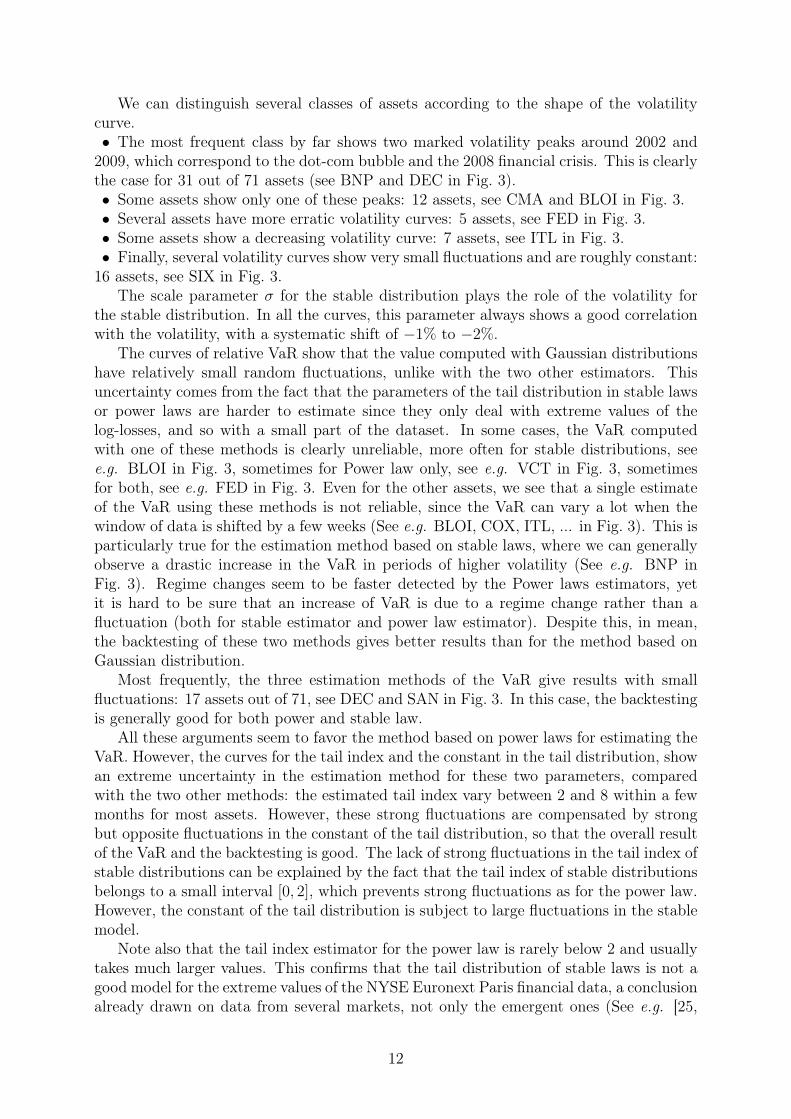
We can distinguish several classes of assets according to the shape of the volatilitycurve.∙ The most frequent class by far shows two marked volatility peaks around 2002 and

2009, which correspond to the dot-com bubble and the 2008 financial crisis. This is clearlythe case for 31 out of 71 assets (see BNP and DEC in Fig. 3).∙ Some assets show only one of these peaks: 12 assets, see CMA and BLOI in Fig. 3.∙ Several assets have more erratic volatility curves: 5 assets, see FED in Fig. 3.∙ Some assets show a decreasing volatility curve: 7 assets, see ITL in Fig. 3.∙ Finally, several volatility curves show very small fluctuations and are roughly constant:

16 assets, see SIX in Fig. 3.The scale parameter 𝜎 for the stable distribution plays the role of the volatility for

the stable distribution. In all the curves, this parameter always shows a good correlationwith the volatility, with a systematic shift of −1% to −2%.

The curves of relative VaR show that the value computed with Gaussian distributionshave relatively small random fluctuations, unlike with the two other estimators. Thisuncertainty comes from the fact that the parameters of the tail distribution in stable lawsor power laws are harder to estimate since they only deal with extreme values of thelog-losses, and so with a small part of the dataset. In some cases, the VaR computedwith one of these methods is clearly unreliable, more often for stable distributions, seee.g. BLOI in Fig. 3, sometimes for Power law only, see e.g. VCT in Fig. 3, sometimesfor both, see e.g. FED in Fig. 3. Even for the other assets, we see that a single estimateof the VaR using these methods is not reliable, since the VaR can vary a lot when thewindow of data is shifted by a few weeks (See e.g. BLOI, COX, ITL, ... in Fig. 3). This isparticularly true for the estimation method based on stable laws, where we can generallyobserve a drastic increase in the VaR in periods of higher volatility (See e.g. BNP inFig. 3). Regime changes seem to be faster detected by the Power laws estimators, yetit is hard to be sure that an increase of VaR is due to a regime change rather than afluctuation (both for stable estimator and power law estimator). Despite this, in mean,the backtesting of these two methods gives better results than for the method based onGaussian distribution.

Most frequently, the three estimation methods of the VaR give results with smallfluctuations: 17 assets out of 71, see DEC and SAN in Fig. 3. In this case, the backtestingis generally good for both power and stable law.

All these arguments seem to favor the method based on power laws for estimating theVaR. However, the curves for the tail index and the constant in the tail distribution, showan extreme uncertainty in the estimation method for these two parameters, comparedwith the two other methods: the estimated tail index vary between 2 and 8 within a fewmonths for most assets. However, these strong fluctuations are compensated by strongbut opposite fluctuations in the constant of the tail distribution, so that the overall resultof the VaR and the backtesting is good. The lack of strong fluctuations in the tail index ofstable distributions can be explained by the fact that the tail index of stable distributionsbelongs to a small interval [0, 2], which prevents strong fluctuations as for the power law.However, the constant of the tail distribution is subject to large fluctuations in the stablemodel.

Note also that the tail index estimator for the power law is rarely below 2 and usuallytakes much larger values. This confirms that the tail distribution of stable laws is not agood model for the extreme values of the NYSE Euronext Paris financial data, a conclusionalready drawn on data from several markets, not only the emergent ones (See e.g. [25,

12

37]). In addition, we observe that the constant of the tail distribution estimated withstable laws is in general greater than the one of the power law. This, combined with thefact that the tail index is almost always smaller for power laws, makes the tail distributionmuch heavier than the one of the power law, and explains the differences in the backtestingof the two methods.

5 Conclusions and perspectivesAlthough a large part of these observations seem to indicate that the power law distri-bution is more suited for VaR estimation, the results of backtesting for stable and powerdistributions remain contrasted. For many assets, the small sample size leads to an im-portant confidence interval containing the 1% target value both for stable and power taildistributions. The assets may also have very different behaviors. But the stocks’ pricesfrom NYSE Euronext Paris could be grouped by similarity of patterns for the price orthe volatility. With the exception of some erratic prices or volatility, the power law pro-vides suitable estimates for the assets within a group. This indicates that the power lawperforms better over a large number of assets.

The finer analysis of the curves associated to the three methods confirms that the VaRestimated by power laws give less excessively small or high values than the other methods.Still, the tail index and constant of the tail distribution show so large fluctuations thatone cannot give confidence to a single estimate of the VaR using this method. One mustrather look at the curve of estimated VaR to try to detect aberrant estimated values ofVaR due to statistical errors.

In any case, the normal distribution is not suitable for dealing with extreme eventsobserved in the markets. Many turbulences and crises arose during the 2001-2011 period,which are clearly seen in prices and volatilities. A difficult question is then to separate“crisis regimes” from “steady-state regime”. This requires to have a clear definition of acrisis. A past crisis may have an important impact on the tail index estimators, both forstable and power law. Conversely, the computation of the VaR based on one-year datain a “steady-state regime” does not anticipate a crisis outbreak. Hence, regime changeindicators and tests, as well as models on probability of occurrence of crises as the onedeveloped by D. Sornette et al. (See e.g. [46]), are needed.

We have considered the prices as independent. Correlations and co-movements mayhappen between stocks. More accurate risk indicators, especially for portfolio manage-ment, should use this information. Regarding extreme events, there are several ways todefine correlations and links between assets. In a future work, we plan to address thisproblem, still by focusing on stock prices, while most of the studies have been performedso far on market indices. There is already large literature on this subject, and we referonly to [39, 55, 73, 75] and related content, among many others.

Even without these potential improvements, the results of the experiments suggest tous that the practitioner can already improve there tools to implement sound risk man-agement based on power law, which appear more adapted than stable and normal distri-butions. Of course, the techniques described in the paper can be refined by consideringcrisis and non-crisis periods, as well as correlation between stocks.

References[1] A. Agresti. “A survey of exact inference for contingency tables”. In: Statist. Sci. 7.1

(1992). With comments and a rejoinder by the author, pp. 131–177.

13

[2] C. Alexander and E. Sheedy. “Developing a stress testing framework based on mar-ket risk models”. In: Journal of Banking & Finance 32.10 (2008), pp. 2220–2236.

[3] V. Andreev, S. Tinyakov, G. Parahin, and O. Ovchinnikova. “An application ofEVT, GPD and POT methods in the Russian stock market (RTS index)”. In: GPDand POT Methods in the Russian Stock Market (RTS Index)(November 17, 2009)(2009).

[4] A. Assaf. “Extreme observations and risk assessment in the equity markets of MENAregion: Tail measures and Value-at-Risk”. In: International Review of FinancialAnalysis 18.3 (June 2009), pp. 109–116.

[5] L. Bachelier. “Théorie de la spéculation”. In: Ann. Sci. École Norm. Sup. (3) 17(1900), pp. 21–86.

[6] J. Beirlant, Y. Goegebeur, J. Teugels, and J. Segers. Statistics of extremes. WileySeries in Probability and Statistics. Theory and applications, With contributionsfrom Daniel De Waal and Chris Ferro. John Wiley & Sons Ltd., 2004.

[7] J. Berkowitz and J. O’Brien. “How Accurate Are Value-at-Risk Models at Commer-cial Banks?” In: The journal of finance 57.3 (2002), pp. 1093–1111.

[8] F. Black and M. Scholes. “The pricing of options and corporate liabilities”. In: TheJournal of Political Economy (1973), pp. 637–654.

[9] R. C. Blattberg and N. J. Gonedes. “A Comparison of the Stable and StudentDistributions as Statistical Models for Stock Prices”. In: The Journal of Business47.2 (1974), pp. 244–280.

[10] C. R. Blyth. “Approximate binomial confidence limits”. In: J. Amer. Statist. Assoc.81.395 (1986), pp. 843–855.

[11] C. R. Blyth. “Correction: “Approximate binomial confidence limits” [J. Amer. Statist.Assoc. 81 (1986), no. 395, 843–855]”. In: J. Amer. Statist. Assoc. 84.406 (1989),p. 636.

[12] P. Boothe and D. Glassman. “The Statistical Distribution of Exchange Rates: Em-pirical Evidence and Economic Implications”. In: Journal of international economics22 (1987), pp. 297–320.

[13] B. O. Bradley and M. S. Taqqu. “Financial risk and heavy tails”. In: Handbookof Heavy Tailed Distributions in Finance. Ed. by S. Rachev. North-Holland, 2003,pp. 35–103.

[14] S. A. Broda, M. Haas, J. Krause, M. S. Paolella, and S. C. Steude. “Stable mixtureGARCH models”. In: Journal of Econometrics 17 (2013), pp. 292–316.

[15] S. D. Campbell. A review of backtesting and backtesting procedures. Tech. rep. 2007,pp. 1–17.

[16] P. K. Clark. “A subordinated stochastic process model with finite variance for specu-lative prices”. In: Econometrica: Journal of the Econometric Society (1973), pp. 135–155.

[17] R. Cont. “Empirical properties of asset returns: stylized facts and statistical issues”.In: Quantitative Finance 1 (2001), pp. 223–236.

[18] R. Cont and J.-P. Bouchaud. “Herd behavior and aggregate fluctuations in financialmarkets”. In: Macroeconomic dynamics 4.2 (2000), pp. 170–196.

14

[19] R. Cont and P. Tankov. Financial modelling with jump processes. Chapman &Hall/CRC Financial Mathematics Series. Chapman & Hall/CRC, Boca Raton, FL,2004.

[20] J. Cotter. “Margin exceedences for European stock index futures using extremevalue theory”. In: Journal of Banking & Finance 25.8 (2001), pp. 1475–1502.

[21] J. D. Curto, J. C. Pinto, and G. N. Tavares. “Modeling stock markets’ volatilityusing GARCH models with Normal, Student’s t and stable Paretian distributions”.In: Statistical Papers 50.2 (July 2007), pp. 311–321.

[22] A. L. M. Dekkers, J. H. J. Einmahl, and L. de Haan. “A moment estimator forthe index of an extreme-value distribution”. In: Ann. Statist. 17.4 (1989), pp. 1833–1855.

[23] D. A. Dickey and W. A. Fuller. “Distribution of the estimators for autoregressivetime series with a unit root”. In: J. Amer. Statist. Assoc. 74.366, part 1 (1979),pp. 427–431.

[24] F. X. Diebold, T. Schuermann, and J. D. Stroughair. “Pitfalls and Opportunities inthe Use of Extreme Value Theory in Risk Management”. In: The Journal of RiskFinance 1.2 (2000), pp. 30–35.

[25] T. Doganoglu, C. Hartz, and S. Mittnik. “Portfolio optimization when risk factorsare conditionally varying and heavy tailed”. In: Computational Economics 29.3-4(Jan. 2007), pp. 333–354.

[26] H. Drees, L. de Haan, and S. Resnick. “How to make a Hill plot”. In: Ann. Statist.28.1 (2000), pp. 254–274.

[27] W. H. DuMouchel. “Estimating the Stable Index 𝛼 in Order to Measure Tail Thick-ness: A Critique”. In: the Annals of Statistics 11.4 (1983), pp. 1019–1031.

[28] W. H. DuMouchel. “On the asymptotic normality of the maximum-likelihood esti-mate when sampling from a stable distribution”. In: Ann. Statist. 1 (1973), pp. 948–957.

[29] P. Embrechts, C. Klüppelberg, and T. Mikosch. Modelling extremal events (Forinsurance and finance). Vol. 33. Applications of Mathematics (New York). Berlin:Springer-Verlag, 1997.

[30] E. F. Fama. “Risk, return, and equilibrium”. In: The Journal of Political Economy791.1 (1971), pp. 30–55.

[31] D. Faranda, V. Lucarini, G. Turchetti, and S. Vaienti. “Numerical convergence ofthe block-maxima approach to the Generalized Extreme Value distribution”. In:Journal of statistical physics 145.5 (2011), pp. 1156–1180.

[32] A. Feuerverger and P. McDunnough. “On efficient inference in symmetric stable lawsand processes”. In: Statistics and related topics (Ottawa, Ont., 1980). Amsterdam:North-Holland, 1981, pp. 109–122.

[33] J. Fleming and B. S. Paye. “High-frequency returns, jumps and the mixture ofnormals hypothesis”. In: Journal of Econometrics 160.1 (Jan. 2011), pp. 119–128.

[34] H. Fofack and J. P Nolan. “Tail behavior, modes and other characteristics of stabledistributions”. In: Extremes 2.1 (1999), pp. 39–58.

15

[35] X. Gabaix. “Power Laws in Economics and Finance”. In: Annual Review of Eco-nomics 1 (Sept. 2008), pp. 255–293.

[36] R. Gençay and F. Selçuk. “Extreme value theory and Value-at-Risk: Relative per-formance in emerging markets”. In: International Journal of Forecasting 20.2 (Apr.2004), pp. 287–303.

[37] M. Gilli and E. Këllezi. “An Application of Extreme Value Theory for MeasuringFinancial Risk”. In: Computational Economics 27.2-3 (2006), pp. 207–228.

[38] A. Gulisashvili. Analytically tractable stochastic stock price models. Springer Fi-nance. Heidelberg: Springer, 2012.

[39] P. Hartmann, S. Straetmans, and C. G. de Vries. “Asset market linkages in crisisperiods”. In: Review of Economics and Statistics 86.1 (2004), pp. 313–326.

[40] B. M. Hill. “A simple general approach to inference about the tail of a distribution”.In: Ann. Statist. 3.5 (1975), pp. 1163–1174. JSTOR: 2958379.

[41] L. C. Ho, P. Burridge, J. Cadle, and M. Theobald. “Value-at-risk: Applying theextreme value approach to Asian markets in the recent financial turmoil”. In: Pacific-Basin Finance Journal 8.2 (2000), pp. 249–275.

[42] R. Huisman, K. Koedijk, C. Kool, and F. Palm. “Fat tails in small sample”. In:Available at SSRN 51141 (1997).

[43] D. W. Jansen and C. G. de Vries. “On the frequency of large stock returns: Puttingbooms and busts into perspective”. In: The review of economics and statistics (1991),pp. 18–24.

[44] R. de Jesús and Ortiz. “Risk in Emerging Stock Markets from Brazil and Mexico:Extreme Value Theory and Alternative Value at Risk Models”. In: Frontiers inFinance and Economics 8.2 (Oct. 2011), pp. 49–88.

[45] R. de Jesús, E. Ortiz, and A. Cabello. “Long run peso/dollar exchange rates andextreme value behavior: Value at Risk modeling”. In: North American Journal ofEconomics and Finance 24 (Jan. 2013), pp. 139–152.

[46] A. Johansen, D. Sornette, and O. Ledoit. “Predicting financial crashes using discretescale invariance”. In: Journal of Risk 1.4 (1999), pp. 5–32.

[47] P. Jorion. Value at Risk: The New Benchmark for Managing Financial Risk. 3rd ed.McGraw-Hill, 2006.

[48] J. Kittiakarasakun and Y. Tse. “Modeling the fat tails in Asian stock markets”. In:International Review of Economics & Finance 20.3 (June 2011), pp. 430–440.

[49] K. G. Koedijk, M. Schafgans, and C. G. de Vries. “The tail index of exchange ratereturns”. In: Journal of international economics (1990).

[50] S. G. Kou. “Chapter 2 Jump-Diffusion Models for Asset Pricing in Financial Engi-neering”. In: Handbooks in Operations Research and Management Science. Ed. byJ. R. Birge and V. Linetsky. Elsevier, 2007, pp. 73–116.

[51] I. A. Koutrouvelis. “An iterative procedure for the estimation of the parameters ofstable laws”. In: Comm. Statist. B—Simulation Comput. 10.1 (1981), pp. 17–28.

[52] K. Kuester, S. Mittnik, and M. S. Paolella. “Value-at-risk prediction: A comparisonof alternative strategies”. In: Journal of Financial Econometrics 4.1 (2006), pp. 53–89.

16

[53] D. Kwiatkowski, P. Phillips, and P. Schmidt. “Testing the null hypothesis of sta-tionarity against the alternative of a unit root: How sure are we that economic timeseries have a unit root?” In: Journal of Econometrics 54 (1992), pp. 159–178.

[54] F. Longin. “The Asymptotic Distribution of Extreme Stock Market Returns”. In:The Journal of Business 69.3 (1996), pp. 383–408.

[55] F. Longin and B. Solnik. “Extreme correlation of international equity markets”. In:The journal of finance 56.2 (2001), pp. 649–676.

[56] M. Loretan and P. Philips. “Testing the covariance stationarity of heavy-tailed timeseries: An overview of the theory with applications to several financial datasets”. In:Journal of Empirical Finance 1.2 (1994), pp. 211–248.

[57] Y. Malevergne, V. F. Pisarenko, and D. Sornette. “Empirical Distributions of Log-Returns: between the Stretched Exponential and the Power Law?” In: QuantitativeFinance 5.4 (2005), pp. 379–401.

[58] Y. Malevergne, V. Pisarenko, and D. Sornette. “On the power of generalized ex-treme value (GEV) and generalized Pareto distribution (GPD) estimators for em-pirical distributions of stock returns”. In: Applied Financial Economics 16.3 (2006),pp. 271–289.

[59] B. Mandelbrot. “The variation of certain speculative prices”. In: Journal of businessXXXVI (1963), pp. 392–417.

[60] R. Marfè. “A generalized variance gamma process for financial applications”. In:Quantitative Finance 12.1 (Jan. 2012), pp. 75–87.

[61] H. Markowitz. “Portfolio Selection”. In: The journal of finance 7.1 (1952), pp. 77–91.

[62] J. H. McCulloch. “Measuring tail thickness to estimate the stable index 𝛼: a cri-tique”. In: J. Bus. Econom. Statist. 15.1 (1997), pp. 74–81.

[63] J. H. McCulloch. “Simple consistent estimators of stable distribution parameters”.In: Comm. Statist. B—Simulation Comput. 15.4 (1986), pp. 1109–1136.

[64] J. Mina and J. Y. Xiao. Return to RiskMetrics: The Evolution of a Standard. Tech.rep. RiskMetrics, 2001.

[65] S. Mittnik and M. S. Paolella. “A simple estimator for the characteristic exponentof the stable Paretian distribution”. In: Math. Comput. Modelling 29.10-12 (1999),pp. 161–176.

[66] J. T. Morisette and S. Khorram. “Exact binomial confidence interval for propor-tions”. In: Photogrammetric engineering and remote sensing 64.4 (1998), pp. 281–282.

[67] Y. Nagahara. “Non-Gaussian distribution for stock returns and related stochas-tic differential equation”. In: Financial Engineering and the Japanese Markets 3.2(1996), pp. 121–149.

[68] J. Nolan. Stable Distributions: Models for Heavy Tailed Data. Boston: Birkhauser,2013.

[69] V. Paulauskas and M. Vaičiulis. Once more on comparison of tail index estimators.Apr. 2011. arXiv: 1104.1242v1.

17

[70] J. I. Pickands. “Statistical inference using extreme order statistics”. In: Ann. Statist.3 (1975), pp. 119–131.

[71] S. Rachev, ed. Handbook of Heavy Tailed Distributions in Finance, Volume 1. North-Holland, 2003.

[72] C. Scarrott and A. MacDonald. “A review of extreme value thresehold estima-tion and uncertainty quantication.” In: REVSTAT–Statistical Journal 10.1 (2012),pp. 33–60.

[73] R. Serfling. “Quantile functions for multivariate analysis: approaches and applica-tions”. In: Statistica Neerlandica 56.2 (2002), pp. 214–232.

[74] W. T. Shaw and M. Schofield. “A model of returns for the post-credit-crunch reality:hybrid Brownian motion with price feedback”. In: Quantitative Finance (Jan. 2012),pp. 1–24.

[75] A. Carvalhal da Silva and B. De Melo Mendes. “Value-at-risk and extreme returns inAsian stock markets”. In: International Journal of Business 8.1 (2003), pp. 17–40.

[76] A. Sing, D. Allen, and P. Robert. “Extreme Market Risk and Extreme Value The-ory”. In: Mathematics and computers in simulation (2012).

[77] Supervision, Basel Committee on Banking, ed. International Convergence of CapitalMeasurement and Capital Standards – A Revised Framework. Bank of InternationalSettlements, June 2004.

[78] G. Ünal. “Value-at-risk forecasts: a comparison analysis of extreme-value versusclassical approaches”. In: The Journal of Risk Model Validation 5.3 (2011), pp. 59–76.

[79] I. Weissman. “Estimation of parameters and large quantiles based on the 𝑘 largestobservations”. In: J. Amer. Statist. Assoc. 73.364 (1978), pp. 812–815.

[80] R. Weron. “Levy-stable distributions revisited: tail index > 2 does not exclude theLevy-stable regime”. In: International Journal of Modern Physics C. 12.2 (2001),pp. 209–223.

18