Embed Size (px)
Citation preview

An Empirical Analysis of the Cost-of-Carry Model
and Istanbul Stock Exchange Futures Contract
Erdem Öncü
Submitted to the
Institute of Graduate Studies and Research
in partial fulfillment of the requirements for the Degree of
Master of Science
in
Banking and Finance
Eastern Mediterranean University
June 2013
Gazimağusa, North Cyprus

Approval of the Institute of Graduate Studies and Research
Prof. Dr. Elvan Yılmaz
Director
I certify that this thesis satisfies the requirements as a thesis for the degree of Master
of Science in Banking and Finance.
Assoc. Prof. Dr. Salih Katırcıoğlu
Chair, Department of Banking and Finance
We certify that we have read this thesis and that in our opinion it is fully adequate in
scope and quality as a thesis for the degree of Master of Science in Banking and
Finance.
Assoc. Prof. Dr. Salih Katırcıoğlu
Supervisor
Examining Committee
1. Prof. Dr. Cahit Adaoğlu
2. Assoc. Prof. Dr. Eralp Bektaş
3. Assoc. Prof. Dr. Salih Katırcıoğlu
iii
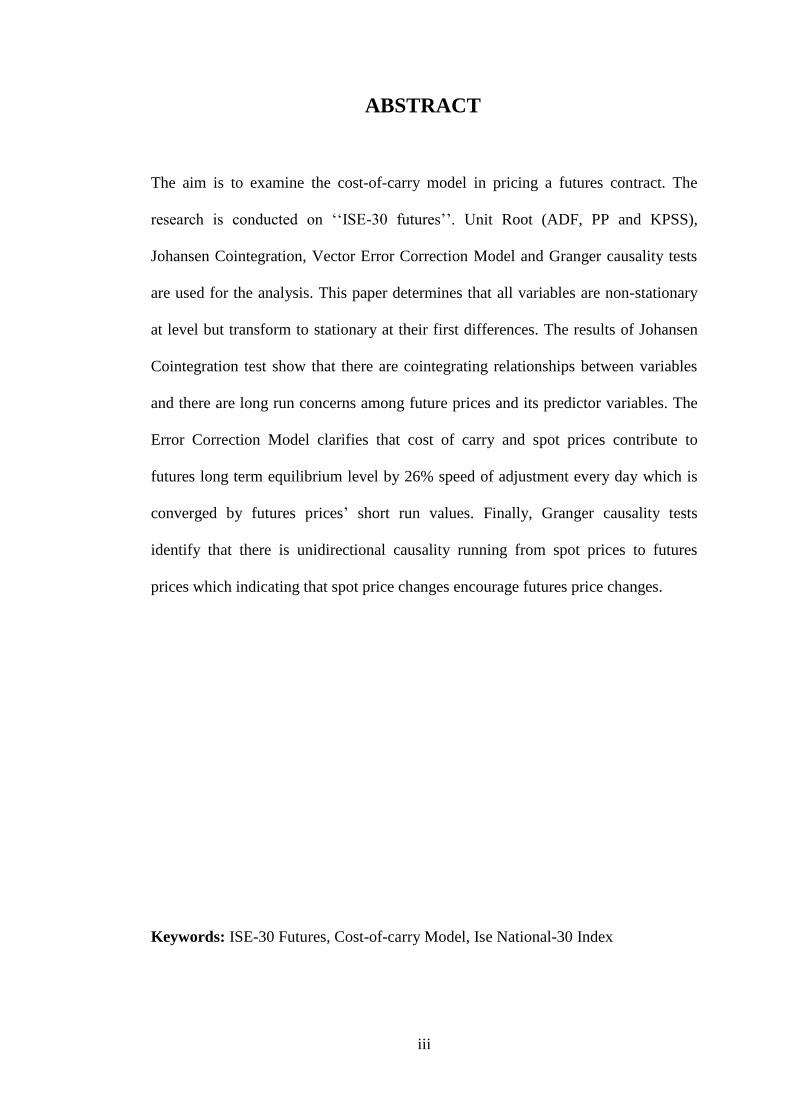
ABSTRACT
The aim is to examine the cost-of-carry model in pricing a futures contract. The
research is conducted on „„ISE-30 futures‟‟. Unit Root (ADF, PP and KPSS),
Johansen Cointegration, Vector Error Correction Model and Granger causality tests
are used for the analysis. This paper determines that all variables are non-stationary
at level but transform to stationary at their first differences. The results of Johansen
Cointegration test show that there are cointegrating relationships between variables
and there are long run concerns among future prices and its predictor variables. The
Error Correction Model clarifies that cost of carry and spot prices contribute to
futures long term equilibrium level by 26% speed of adjustment every day which is
converged by futures prices‟ short run values. Finally, Granger causality tests
identify that there is unidirectional causality running from spot prices to futures
prices which indicating that spot price changes encourage futures price changes.
Keywords: ISE-30 Futures, Cost-of-carry Model, Ise National-30 Index

iv
Öz
Bu çalışmanın amacı, taşıma maliyeti modelinin vadeli işlem sözleşmesi
fiyatlandırmasını araştırmaktır. Çalışma IMKB-30 vadeli işlem sözleşmesi üzerine
yapılmıştır. Birim Kök (ADF, PP and KPSS) testleri, Johansen Eşbütünleşme testi,
Vektör Hata Düzeltme Modeli ve Granger nedensellik testi analizlerde kulanılmıştır.
Bu çalışma gösteriyor ki, tüm değişkenler durağan olmayan bir halden fark alma
yöntemi ile durağan hale gelmiştir. Johansen Eşbütünleşme testi sonuçlarına göre,
değişkenler arasında eşbütünleşme ilişkisi vardır ve uzun dönemli ilişki vadeli
fiyatlar ve vadeli fiyatları açıklayıcı değişkenler arasında görülmektedir. Vektör Hata
Düzeltme Modeli açıklamasına göre, Vadeli fiyatlar, Spot fiyatlar ve Taşıma
maliyetinin etkisiyle uzun dönem denge değerlerine %26 hızla ulaşmaktadır. Son
olarak, Granger nedensellik test açıklar ki, Spot fiyatlardan Vadeli fiyatlara doğru tek
yönlü bir nedensellik vardır bu demek oluyor ki, Spot fiyatlardaki değişim Vadeli
fiyatlardaki değişimi olumlu yönde etkiler.
Anahtar Kelimeler: IMKB-30 vadeli sözleşmeleri, Taşıma maliyeti modeli, IMKB-
30 Endeksi

v
To my family

vi
ACKNOWLEDGMENTS
I would like to thank to my supervisor Assoc. Prof. Dr. Salih Katırcıoğlu for his
continuous guidance, support and encouragement in the preparation of this thesis.
I also would like to thank Nigar Taspınar for answering my endless questions.
I would like to express my special thanks to my family for their invaluable and
continuous support throughout my studies and my life. I also would like to thank you
my little brother, Emre Öncü, who encouraged me to fight with this hard work.

vii
TABLE OF CONTENTS
ABSTRACT ................................................................................................................ iii
ÖZ ............................................................................................................................... iv
DEDICATION ............................................................................................................. v
ACKNOWLEDGMENTS .......................................................................................... vi
LIST OF TABLES ...................................................................................................... ix
LIST OF FIGURES ..................................................................................................... x
LIST OF ILLUSTRATONS ....................................................................................... xi
LIST OF ABBREVIATIONS .................................................................................... xii
1 INTRODUCTION .................................................................................................... 1
1.1 Background ........................................................................................................ 1
1.2 The Turkish Case ............................................................................................... 3
1.3 Aim and Importance of the Study ...................................................................... 3
1.4 Structure of the Research ................................................................................... 4
2 THEORETICAL CONSIDERATIONS AND EMPIRICAL STUDIES .................. 5
2.1 Theoretical Considerations ............................................................................... 5
2.2 Empirical Studies ............................................................................................... 6
3 INVESMENT ENVIRONMENT IN TURKEY ....................................................... 9
3.1 The Turkish Economy in General ...................................................................... 9
3.2 Major Factors of Foreign Entity in Turkey ...................................................... 12
3.3 Turkish Derivatives Exchange ......................................................................... 13
4 DATA AND METHODOLOGY ............................................................................ 17
4.1 Data .................................................................................................................. 17
4.2 Methodology .................................................................................................... 17

viii
4.2.1 Empirical Model ........................................................................................ 17
4.2.2 Unit Root Tests ......................................................................................... 18
4.2.3 Co-integration Tests .................................................................................. 19
4.2.4 Error Correction Model ............................................................................. 21
4.2.5 Granger Causality Tests ............................................................................ 22
5 ECONOMETRIC RESULTS ................................................................................. 23
5.1 Unit Root Test for Stationarity......................................................................... 23
5.2 Co-integration Analysis ................................................................................... 24
5.3 Level Coefficients and Error Correction Model Estimation ............................ 25
5.4 Granger Causality Test..................................................................................... 27
6 CONCLUSION AND POLICY IMPLICATIONS ................................................. 29
5.1 Conclusion ...................................................................................................... 29
5.2 Implications ..................................................................................................... 30
REFERENCES ........................................................................................................... 31

ix
LIST OF TABLES
Table 5.1: ADF, PP and KPSS Tests for Unit Root ................................................... 24
Table 5.2: Johansen Co-integration Test .................................................................... 25
Table 5.3: Error Correction Model............................................................................. 26
Table 5.4: Granger Causality Tests under Block Exogeneity Approach ................... 28

x
LIST OF FIGURES
Figure 3.1: GDP (Current prices) and GDP (Constant prices) 2009-2012 ................ 10
Figure 3.2: How Turkey and comparator economies rank on ease of getting credit . 11
Figure 3.3: Total Trading Value of Ise-30 Futures 2005-2011 .................................. 16

xi
LIST OF ILLUSTRATIONS
Illustration 3.1: TEOS Order Menu ........................................................................... 14

xii
LIST OF ABBREVIATIONS
ADF test Augmented Dickey-Fuller test
AIC Akaike Information Criteria
GAFTA Grain And Feed Trade Association
KPSS test Kwiatkowski–Phillips–Schmidt–Shin
PP test Phillips-Perron test
SIC Schwartz Information Criterion
TEOS Turkdex Exchange Operations System
TurkDex Turkish Derivatives Exchange
VECM Vector Error Correction Model

1
Chapter 1
INTRODUCTION
1.1 Background
Notion of risk management has resulted from the rampant changes in the interest
rates, especially in the rates of exchange, which have been following since the 1970s
as consequence of the exchange of the Bretton Woods System based on the pegged
exchange rate regime with the fluctuating exchange rate. According to Richter and
Sheble (2007), nowadays, many financial market participants try to reduce their risk
with low cost. This happening leads to increasing in demand for investment and risk
management. Futures constitute major part of risk management. Futures Market is
the one which have surfaced as a consequence of the need for risk management.
Futures Markets are those which have significant functions in the integration with the
developed international markets. First, futures market started to operation in the
United States in 1982 than financial futures markets were quickly introduced in
countries outside the United States.
Today, futures trading play considerable role in the global financial system. Futures
markets transference of risk function and price discovery function help people to
make more safety, lucrative and efficient investment decisions. Trading in futures
markets bring some advantages over trading spot markets. Also futures contracts
ensure risk transfer and hedging risks. Fund managers prefer to use futures actively
in order to achieve an optimal combination of risk.

2
Since the beginning of United States stock index futures in 1982, mutual effect of
stock market spot price and stock market future price have been scope of
investigation. Cost-of-Carry model is a norm model of futures pricing. It describes
the relationship between the future price and the current cash price of an asset.
Literature consist many studies which analyzes the relationship among stock spot
price of stock market and stock market future price from different perspectives.
According to Thongtip (2010), four basic assumptions can explain cost-of-carry
model extremely well. First one is market should be perfect. Perfect market involves
no transaction cost, taxes and no constraint on short sales. Second one is there is no
limitation on lending or borrowing at the same risk. Third one is costless storage.
Assets do not depreciate with storage and can be stored costless. The last one is the
risk free rate should be certain.
Thongtip (2010) supported that arbitrage is major problem of cost-of-carry model
and the equation is quitely reflected by arbitrage transactions. Cost-of-carry model is
only valid without arbitrage. Arbitrage can be defined as synchronous buy and sale
of an asset for earning profit from a difference in the price. The model cost-of-carry
defines the arbitrage free price of derivative contracts. It creates sustainable
replicating position of derivative contract in the spot markets and keeping this
replication position over the life of the derivative contract. Thongthip (2010) states
that price changes must constitute a trend in the other price for holding prices in
orientation with the model of Cost-of-carry.
Costs of carry model assume that market is perfect and arbitrage is not viable. But, in
the real world we can face some mispricing opportunities. According to Sutcliffe
3
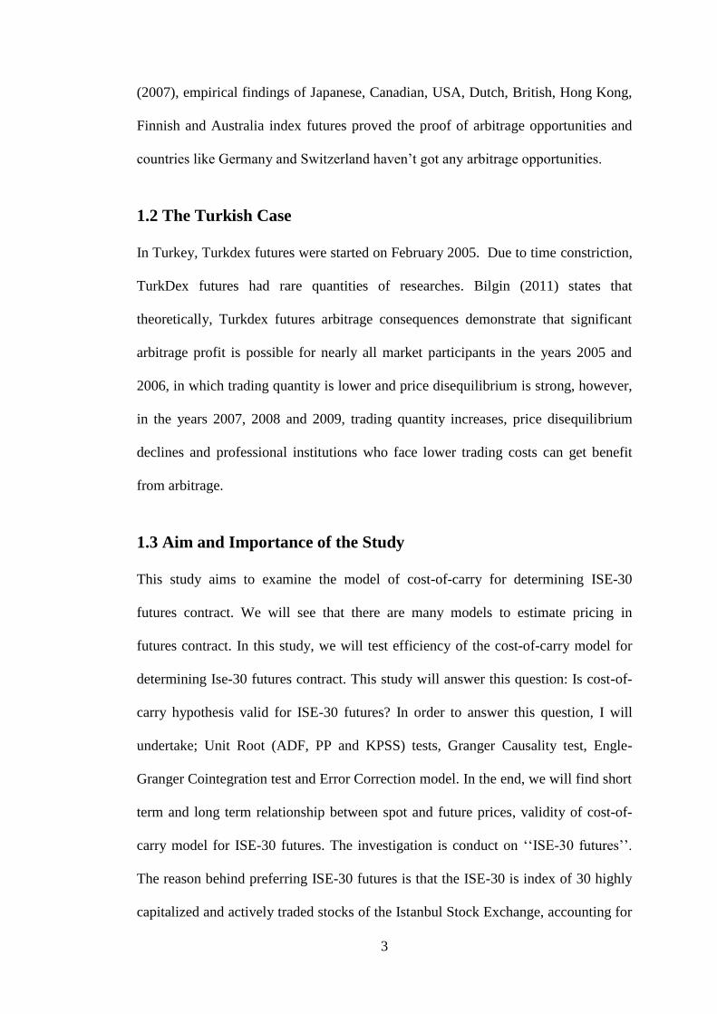
(2007), empirical findings of Japanese, Canadian, USA, Dutch, British, Hong Kong,
Finnish and Australia index futures proved the proof of arbitrage opportunities and
countries like Germany and Switzerland haven‟t got any arbitrage opportunities.
1.2 The Turkish Case
In Turkey, Turkdex futures were started on February 2005. Due to time constriction,
TurkDex futures had rare quantities of researches. Bilgin (2011) states that
theoretically, Turkdex futures arbitrage consequences demonstrate that significant
arbitrage profit is possible for nearly all market participants in the years 2005 and
2006, in which trading quantity is lower and price disequilibrium is strong, however,
in the years 2007, 2008 and 2009, trading quantity increases, price disequilibrium
declines and professional institutions who face lower trading costs can get benefit
from arbitrage.
1.3 Aim and Importance of the Study
This study aims to examine the model of cost-of-carry for determining ISE-30
futures contract. We will see that there are many models to estimate pricing in
futures contract. In this study, we will test efficiency of the cost-of-carry model for
determining Ise-30 futures contract. This study will answer this question: Is cost-of-
carry hypothesis valid for ISE-30 futures? In order to answer this question, I will
undertake; Unit Root (ADF, PP and KPSS) tests, Granger Causality test, Engle-
Granger Cointegration test and Error Correction model. In the end, we will find short
term and long term relationship between spot and future prices, validity of cost-of-
carry model for ISE-30 futures. The investigation is conduct on „„ISE-30 futures‟‟.
The reason behind preferring ISE-30 futures is that the ISE-30 is index of 30 highly
capitalized and actively traded stocks of the Istanbul Stock Exchange, accounting for

4
70 percent of Turkey‟s market volume. Furthermore, only ISE-30 futures are
executed in United States Futures Market from ISE futures.
1.4 Structure of the Research
This research contains six chapters. First chapter involves exhaustive information
about futures and cost-of-carry model. Chapter two presents theoretical and empirical
literature. Chapter three contains detailed data about investment background of
Turkey. Data and methodology of econometric analysis is devoted in chapter four.
Econometrics results are introduced in fifth chapter. In the end, chapter six concludes
the findings.

5
Chapter 2
THEORETICAL CONSIDERATIONS AND EMPIRICAL
STUDIES
2.1 Theoretical Considerations
Kolb and Overdahl (2007) found that future value affiliates on the spot value of a
good and the cost of stocking the underlying commodities from the present to the
futures contract‟s end of the maturity date. It can be expressed in the following
equation.
Ft = St (1+Ct) (1)
In equation (1), Ct is the cost of carrying commodity from present to the delivery date
of the futures contract, Ft is the futures price and St is the spot price at time t.
Amin and Jarrow (1991) used framework of the Heath et al. (1992) and undertook a
study on creating general framework to price contingent claims on foreign
currencies. Brenner and Kroner (1995) worked on futures markets and find that
stochastic interest rates and asset prices are connected to marking-to-market term.
Also, they took the natural logarithm of model of Heath et al. (1992) and found linear
relationship between the logarithms of the spot price, future price and differential.
Helmer and Longstaff (1991) improve a closed-form general equilibrium model of
stock index future prices in a continuous-time economy touched by stochastic
interest rates and market volatility. Their model ignores the taxes and the transaction

6
costs as well as other market defects. Therefore, Hsu and Wang (2004) studied
incomplete arbitrage mechanism under imperfect market. The model can be
expressed as:
1 T t , ( – ) au
F S t St Dt e
,
where 1 [ ] / (1 )
p p
a pu u u
.
Where Ft and St are the futures and spot price respectively; is the value
expectancy coefficient; μp and μ are permanent yield of the stock index, the
instruments involving of the underlying stocks and futures contracts changes a σp = 0
and completely hedged portfolio.
2.2 Empirical Studies
There are many studies that have been done in this area but big parts of them are
established on advanced markets like the U.S. Limited studies have been done in
other markets. Kawaller et al. (1987) examined intraday price concerns among the
futures contract of S&P 500 and the index of S&P 500 and revealed that the futures
price changes guide the cash market by among twenty and forty-five minutes. Their
findings show that when volatile index infrequently impressed futures over one
minute, futures price changes led index movement from 20 to 45 minutes. Brenner
and Kroner (1995) states that co-integration among futures and cash prices affiliate
the time-series characteristic of cost of carry. Crowder and Phengpis (2005) carried
on studies of Brenner and Kroner (1995). He finds that futures and cash prices are
co-integrated and there is stable cointegrating relationship among cost of carry yields
and three month Treasury bill rate.

7
Hemler and Longstaff (1991) studied futures contract of NYSE from 1982 to 1987.
Their main conclusion is that stock index future prices are concerned to market
volatility. Also, they argue that cost of carry model results is weaker than general
equilibrium. General equilibrium model assume that all prices are walking around
the market equilibrium point. However, some studies have contradicted results. For
example, Yu Lu (2011) studied the relationship among the spot market and futures
market of Hong Kong during the sample period January 2nd 2007 through February
26th 2010. He found that cost of carry model better than general equilibrium and
expectation models.
Wang (2007) tried to develop the cost-of-carry model during the sample period from
1997 to 2005. His consequences clarify that identifying the degree of market defects
plays major role when selecting a pricing model to estimate the theoretical values of
stock index futures. Hsu and Wang (2006) compared the cost of carry model and
other developed models. Their data comprise 1998 to 2004. Their main finding is
that cost of carry model has weaker performance than Hemler and Longstaff model
and the Hsu–Wang model. Later, Wang (2009) carried on Hsu and Wang (2006)
research. He found that cost of carry model provide weaker performance than
Hemler and Longstaff model and the Hsu–Wang model. But, the model of cost of
carry provides sufficient performance in the Nikkei 225 futures market.
Sequeira and McAleer (2000) investigated cost of carry model and they run unit root
and cointegration tests. Results of tests provide considerable contribution for pricing
of Australian dollar futures contracts. Also, Jackline and Deo (2011) examined the
relationship between the futures market and spot market of S&P CNX Nifty during
8
the sample period January 2003 through September 2010. Their findings show that
price discovery was reached first in the spot market and the futures price series had a
better speed of adjustment to the previous deviations.
We can see that traders rarely invest on futures in the emerging markets. Modern
example, Lucian (2008) studied on lead-lag relationship Romanian cash market and
futures market. According to him, short selling stock is not allowed in the Romanian
cash market. At the same time, usage of arbitrage or hedging is significantly low.
In case of ISE 30 futures, Zeynel (2008) investigates the relationship between ISE 30
futures and ISE 30 spot prices and hedge ratios. The daily data covers the period
from January 2005 to December 2007. She found that hedging with futures provides
substantial advantage in Turkish market. Also, Bilgin (2011) studied on arbitrage
between the ISE-30 stock index contract of TURKDEX and underlying ISE-30 stock
index. He concludes that significant arbitrage is available for nearly all market
participants in years 2005 and 2006.
9
Chapter 3
INVESMENT ENVIRONMENT IN TURKEY
3.1 The Turkish Economy in General
Turkey have started structural adjustment program in 1980. Most important element
of this program is financial liberalization. In other words, globalization of financial
system was crucial for development of Turkey. Financial liberalization program
designed to solve turkey‟s internal and external disequilibrium problems. Firstly,
liberalization period started with determination of foreign exchange rates which were
liberalized and quota and licensing system was abolished. In 1994, banking and
currency crisis started in Thailand and Mexico. Turkey lived effects of crisis very
sharply. Central Bank of Turkey lost half of its international reserves and interest rate
raised to three digit levels. Custom union agreement was signed in December 1995 to
expand trade, proximity between Turkey and Europe. In August 1999, Turkey was
hit by big earthquake that hit also economy. Turkey saw devastating face of crisis
and established BRSA (Banking Regulation and Supervision Agency) in order to
approach the task of auditing the sector in single hand.
Most of accounting rules are changed and sector becomes more profitable. Also,
Turkey enrolled the IMF programs in 2001 and Economic growth was revived Now,
Turkey‟s dynamic economy has complex mix of contemporary industry and
commerce. Banking, transport and communication sectors are playing major role in
rapidly growing private sector of Turkey. Main advantages of Turkey are high

10
growth and stable economy, young aged population, geographical benefits and
structural reforms. Istanbul is largest city in the Middle East and Balkans. Recently,
Istanbul is becoming significant actor in the global economy. EU picked Istanbul for
“European Capital of Culture 2010”. Now, Turkey is member of many international
organizations these are; the International Chamber of Commerce (ICC), D-8, Council
of Europe, World Trade Organizations (WTO), Economic Cooperation Organization
(ECO), the United Nations Conference on Trade and Development (UNCTAD), the
Organization of the Black Sea Economic Cooperation (BSEC), the World Customs 8
Organization (WCO). Economic power and military power make Turkey important
country in Eastern Europe and Asia.
Figure 3.1 GDP: (Current prices) (Million TL) and GDP (Constant prices) (Million
TL)
Source: TURKSTAT (2013)

11
Turkey enjoyed adequate economic performance between IV. quarter 2009 and IV.
quarter 2012 with 44 percent of GDP (Current prices) growth. In 2012 Turkey‟s
GDP was $ 794,468 million, which shows that Turkey‟s GDP is increasing rapidly.
According to Anadolu Agency (2013) Turkey stands at rank 2 with its economic
growth rate following Estonia in the Euro zone. Turkish economy has expanded
since final quarter of 2009 despite the global economic crisis. When we compare
Turkey gdp growth rate and countries of Euro zone gdp growth rates, Turkey‟s gdp
growth rates was higher than most of the developing and developed European
countries since final quarter of 2009. Recent findings show that Turkey is reached
elites of Europe Countries.
Figure 3.2: How Turkey and comparator economies rank on ease of getting credit
Source: Doing Business (2013)

12
According to Doing Business report 2011 Turkey has improved ease of getting credit
with new law and it was ranked as 65. Now, Turkey stays at 83 in the ranking of 185
economies rank on ease of getting credit (figure 3.2). We can see that reforms of
financial development of Turkey have decelerated since 2011.
3.2 Major Factors of Foreign Entity in Turkey
Pull and push factors are playing major role for investing. From Turkey point of
view, i will examine pull and push factors. Many advantage of Turkish financial
system lures foreign participants. Pull factors can be classified with 4 groups. First
one is economic indicators. Population increases, per capital income, interest rates
and inflation rates are all symbolize value of economic indicators. Second one is
„‟Reform‟‟ policies. EU accession process started 2005 and results make the foreign
investors satisfied. Third one is development of system. After the crises, Turkey
decides to change system, many reforms applied and exchange rate system is
changed. The last one is product differentiation. In Turkey, Banks have large variety
of products and it attracts foreign customers. Modern example, National bank of
Greece bought Finansbank because of Finansbank car credits.
Liberalization of financial sector has limitation. Such as low profit margin, low
variety product, political diseases deters foreign participants. Moreover, regulatory
restrictions at home also affect foreign participation ratio. Main push factor in
Turkey is political diseases. There have been 59 different governments in the 83-year
history of Turkish Republic and it shows high political risk. Positive environment of
sector can be change suddenly with political shock which it is very familiar situation
for Turkey. We also consider public confidence to push factor. In my opinion, one of
decent push factor is religion. All Christian based countries have excessive

13
Christians. Clearly, we can say more than %2 percent of world heavily reject invest
at Muslim countries. But, many investor support the idea of money is the wise man‟s
religion.
Rather than pull or push factors, other countries are also being important factor.
Since 20 years, many rules have been occupied the place of free investment.
Organizations like WTO, agreements like GAFTA break the rules. Now people can
invest foreign countries freely. The growth rates in the developed countries have
been very poor during last 10 years. For example, average growing rate of EU
banking sector %1 in last 10 years. Turkey also offers high profit margin with low
risk of default. In this regard, Turkey is one of the best alternatives for foreign
entrepreneurs. But, still Turkey has foreign debt problem. More than half GNP of
Turkey is foreign debt and most of it long term.
3.3 Turkish Derivatives Exchange (TurkDex)
In 1989, first studies were started for establishing futures market. In these studies,
agricultural products play major role. Then, studies carried on project of Turkey
capital market modernization in 1991. In the end, futures part of Turkey capital
market modernization failed. In 1995, second attempts were started for establishing
future market. In 1997, Istanbul Gold Exchange started to operate gold futures. In
2001, Istanbul Stock Exchange started to operate currency future contracts. In 2005,
rights for operating futures transferred to TurkDex.
TurkDex is ”the Turkish Derivatives Exchange” which began to operate in İzmir on
February 4, 2005 with 34 members. It offers financial and commodity instruments.
Its main priority is to improve and provide derivatives to help traders, hedgers,

14
speculators and investors to decrease their risks actively. TurkDex is a private
corporation and shareholders of TurkDex well-known institutions of Turkey. Major
shareholders of Turkdex are The Union of Chambers and Commodity Exchanges of
Turkey (25%), Istanbul Stock Exchange (18%) and Izmir Mercantile Exchange
(17%). Exchange may unilaterally close all or some part of open positions in case of
war, natural disaster, government intervention to the prices and similar cases.
Takasbank undertake all clearing actions. Takasbank behaves like to buyer to every
seller, and the seller to every buyer. Takasbank guarantees settlement of transactions
and behaves as central counterparty. But the guarantee is limited and equal to the size
of the guarantee fund.
Illustration 1.1: TEOS Order Menu
Source: Vadeli Opsiyonlar Borsası (Turkish Derivatives Exchange) (2013)

15
TurkDex uses computer software program for executions. Program name is TEOS.
TEOS subsystems are electronic trading and matching system, market reporting and
monitoring system, margin verification and risk calculation system and security
administration system. TEOS is a structure that involves an electronic order
matching system and remotely accessible network. Database, Trading Engine and
Trader Workplace are main parts of TEOS. Database contains information and
parameters and reports. Order matching and managing risks can be done in Trading
Engine. Trader Workplace provides connection between clients and Trading Engine.
The software contains requirements of Turkish financial system and Turkdex.
Most popular contracts in 2005 and 2006 were currency futures contracts and ISE-30
futures contracts were most popular contracts in 2007, 2008 and 2009.TurkDEX is
one of the world fastest developing derivatives exchange. Today, major derivatives
exchanges contain TurkDex. TurkDEX future contracts are in transparent platform
and very liquid. The most liquid financial instrument of Turkish capital markets is
the ISE-30 equity index futures. Trading daily average value is about 1.2 billion
USD. TurkDEX collateralized 732 million USD in April 2011 for managing risk. It
adjusted margin levels regularly.
Turkdex ISE-30 futures total trading value is given as Fig 3.3. As can be seen in
Figure 3.3, ISE-30 futures have positive trend until 2011 and we can see little
decrease in 2011. In this thesis, study is conducted on „„ISE-30 futures‟‟. ISE-30 is
index of 30 highly capitalized and actively traded stocks of the Istanbul Stock
Exchange, accounting for 70 percent of Turkey‟s market volume.

16
Figure 3.3: Total Trading Value of ISE-30 Futures (in millions of USD)
Source: TurkDex (2011)
Furthermore, only ISE-30 futures are executed in United States Futures Market from
ISE futures. From ISE-30 point of view, foreign investors have not any regulatory
restrictions and tax duty. All types of investors are lured by the small contract size of
ISE-30 futures (about 4.000 USD).
0
50,000
100,000
150,000
200,000
250,000
300,000
2005 2006 2007 2008 2009 2010 2011
TurkDex Ise-30 Futures Yearly Total Trading Value (in millions of USD)

17
Chapter 4
DATA AND METHODOLOGY
4.1 Data
ISE-30 is index of 30 highly capitalized and actively traded stocks of the Istanbul
Stock Exchange. The Ise-30 futures traded at the Turkish Derivatives Exchange
(TurkDex). Daily data used in this study and have been taken from archives of
TurkDex, Istanbul Stock Exchange and Central Bank of the Republic of Turkey
(2013). The data contains eighteen Ise-30 futures series from the 1th
of January 2010
to the 31th
of December 2012. Also, risk free interest rate is used to find out a cost of
carry. In this study, overnight repo rates (repurchase rate) are used as risk free rates.
4.2 Methodology
In this study, five models of analysis were derived. First, the Augmented Dickey-
Fuller (ADF), Philips-Perron (PP) and Kwiatkowski–Phillips–Schmidt–Shin (KPSS)
unit root tests were undertaken. Second, Johansen co integration test was employed
to test long run relationship between spot prices and futures prices. Lastly, Granger
Causality tests were undertaken to specify direction of causality among the variables.
4.2.1 Empirical Model
Since the beginning of stock index futures in the United States in 1982, there are
many studies in the finance literature have attempted to clarify the specifications of

18
future pricing. Cost of carry model describes the relationship between the future
price and the current spot price of an asset.
t t tF F S , C (1)
In this equation, futures price (Ft) is the function of cost of carry (Ct) and spot price
(St).
f d t ,T
r r . q
t,T tF S .e
(2)
Ft refers future price, St refers spot price, rf represents risk free rate, rd is dividend
yield and qt,T refers marking to market feature. We can describe cost carry model
econometrically with the following equation (Tharavanij, 2012):
t,T 1 2 f 3 tF .St r . . (3)
According to Tharavanij (2012), the model can enforce several limitations. These
are: α= q and β1=1, β2=1, β3= -rd when rd and qt, τ are approximately fixed.
4.2.2 Unit Root Tests
In economy, many variables are non-stationary. The presence and form of non-
stationary have detected by unit root tests. Why do we need to test for non-
stationary? Because, we need to know series are stationary before the estimating
economic model and making co integration test. According to Gujarati (2003),
Dickey – Fuller test does not work when ut are correlated. Therefore, Dickey and
Fuller developed Augmented-Dickey Fuller (ADF). Augmented-Dickey Fuller
(ADF) test is well known and it is valid in large samples. ADF test showed in the
following model.

19
p
i
titjtt ytayay2
1210 (4)
Katırcıoglu et al (2007) found that where y is the series; t = time (trend factor); α =
constant term (drift); εt = Gaussian white noise and p = the lag order. Akaike
Information Criteria (AIC) chose the number of lags “p” in the dependent variable to
ensure that the errors are white noise. The alternative hypothesis (H1) clarifies that
the series is stationary whereby the null hypothesis (H0) represents that series is non-
stationary. Philips-Perron test is used to test the null hypothesis in the time series
analysis. The Philips-Perron t-statistic computed as
( )
(5)
In this equation α is the standard error of the test regression and tb, tsb is the t-statistic
and standard error of β. Main advantage of Philips-Perron test is that Philips-Perron
tests are robust to unspecified autocorrelation and general forms of heteroscedasticity
in the error term ut. Kwiatkowski–Phillips–Schmidt–Shin (KPSS) tests are used to
test null hypothesis and observe time series is stationary around a deterministic trend.
The KPSS test statistic of the null level stationary is:
2
21
ˆ1
,u
n
tTt
KPSS s
(6)
where St=∑ j and ut is the residual regression of a regression Yt. The KPSS is
most commonly used stationary test.

20
4.2.3 Co-integration Tests
According to Gujarati (2003), co-integration clarifies longrun equilibrium
relationship between series. For example, separately, logarithmic domestic
production and logarithmic domestic consumption are not covariance stationary. But,
they are stationary together that means they are cointegrated. Eagle-Granger two step
method allows one cointegrating relationship. But, the Johansen test allows more
than one cointegrating relationship.
Cheung and Lai (1993) found that the maximum eigen value test for cointegration is
weaker than the trace test. Engle and Granger (1987) proposed the simple following
two-step estimator. First step is determining static cointegrating relationship. Second
step is estimating the error correction model. Katırcıoglu et al (2007) clarify that
there are problems which stems from Engle and Granger (1987) procedure and
Johansen (1988) test is the more reliable test to avoid problems. VAR model
represented in the following equation:
tKtKtt eXXX ...11 (for t=1, …T) (7)
In this equation, Xt, Xt-1, …, Xt-K are vectors of current and lagged values of P
variables respectively which are known as I(1) in the model; matrices of coefficients
with (PXP) dimensions are Π1,….,ΠK ; μ is an intercept vector1; and et is a vector of
random errors (Katırcıoglu et., 2007). The assumption established the number of
lagged variables that error terms are not auto correlated. The number of co-
integrating relationship(s) (i.e. r) which is determined by testing whether its Eigen
values (λi) are different from zero is showed by the rank of Π. According to
Katırcıoglu et al (2007), using the Eigen values of Π ordered from the largest to the
smallest is for computation of trace statistics2 that is proposed by Johansen (1988)

21
and Johansen and Juselius (1990). Trace statistic (λtrace) is computed by the
following formula3:
)1( itraceLnT , i = r+1, …, n-1 and the null hypotheses are : (8)
H0: r = 0 H1: r ≥ 1
H0: r ≤ 1 H1: r ≥ 2
H0: r ≤ 2 H1: r ≥ 3
4.2.4 Error Correction Model
Engle and Granger (1987) clarified that Granger representation theorem, states that
the relationship between X and Y variables can be expressed as ECM (Error
Correction Model) if X and Y variables are cointegrated. ECM model of cost of carry
model is:
3
t t,T 0 1 t 2 3,Q 1 QZ lnF a a lnS a a
QD
(9)
1 μ is a vector of I(0) series and represent dummy variables. This ensures that errors et are white
noise. 2 Asymptotic critical values of Osterwald-Lenum (1992) are used in this study.
3 Firstly, we test the null hypothesis that there are not any co-integrating relationships. The alternative
hypothesis (i.e. s ≤1, …, s ≤ n) are to be tested sequentially if null hypothesis is rejected,. Cannot be
rejected in the first place if s=0, it clarifies that independent variables and dependent variable haven‟t
any cointegrating relationship.

22
In the above mentioned model, Zt is the deviation from long run equilibrium.
Thongtip (2010) conclude that if Zt=0, the futures and spot prices are called to be in
long equilibrium.
4.2.5 Granger Causality Test
Clive Granger won Nobel Prize in Economics with Granger Causality test. The
Granger Causality test is identifying that one time series is useful in forecasting
another or not. Granger Causality tests need a Vector Error Correction Mechanism
(VECM) if there is cointegration relationship (Katırcıoglu et al., 2007). Cost of carry
model Vector Error Correction Mechanism (VECM) can be shown as:
1h h2
t,T 1 Ft 1 11.i t i,T 12, j t j 1,t
1 2
lnF a y lnF lnSi j
(10)
1h h2
t,T 1 Ft 1 21.i t i,T 22, j t j 2,t
1 2
lnF y lnF lnSi j
(11)
Thongtip (2010) mention that using the Engle-Granger methodology or Johansen
methodology on cost of carry model expressed the (FT,t) and (St) series are co-
integrated of order (1).

23
Chapter 5
ECONOMETRIC RESULTS
5.1 Unit Root Test for Stationarity
Augmented-Dickey Fuller (ADF), Philips-Perron, Kwiatkowski–Phillips–Schmidt–
Shin (KPSS) tests are used to test stationary of variables. All tests are mentioned in
chapter 4. Tests have been executed at level and first difference which can be seen in
Table 5.1.
According to result of ADF, PP, KPSS tests, these tests have estimated different
conclusions. KPSS test is robust than other tests. Therefore, we should accept
consequences of KPSS test. KPSS test clarifies that all variables are non-stationary at
level but become stationary at their first differences. Empirical model is explained in
the chapter 4 which is supported by consequences of tests. Tables 5.1 express the
consequences of ADF, PP, KPSS tests.

24
Table 5.1: ADF, PP and KPSS tests for Unit Root
Statistics (Level) ln Spot price lag ln Future price lag Cost of carry lag
T (ADF) -1.58 (0) -1.6 (0) -7.1* (0)
(ADF) -1.36 (0) -1.38 (0) -7.1* (0)
(ADF) 0.85 (0) 0.82 (0) -3.61* (1)
T (PP) -1.55 (8) -1.64 (5) -7.27* (9)
(PP) -1.34 (8) -1.43 (5) -7.27* (9)
(PP) 0.89 (10) 0.83 (7) -3.8* (1)
T (KPSS) 0.34*** (22) 0.34*** (22) 0.144** (20)
(KPSS) 0.40** (22) 0.41** (22) 0.137 (20)
Statistics (Level) ∆ln Spot price lag ∆ln Future price lag ∆Cost of carry lag
T (ADF) -27.73* (0) -27.05* (0) -17.58* (2)
(ADF) -27.73* (0) -27.05* (0) -17.59* (2)
(ADF) -27.72* (0) -27.04* (0) -17.60* (2)
T (PP) -27.75* (10) -27.05* (8) -30.58* (10)
(PP) -27.74* (9) -27.05* (8) -30.60* (10)
(PP) -27.73* (9) -27.04* (7) -30.62* (10)
T (KPSS) 0.10 (10) 0.094 (8) 0.013 (10)
(KPSS) 0.13 (10) 0.12 (7) 0.013 (10)
Note:
Spot price represents spot price of ISE-30 index; Future price is the future prices of ISE-30 index
futures; Cost of carry represents the cost of carry underlying asset to maturity (rf.τ). All of the series
are at their natural logarithms. T represents the most general model with a drift and trend; τμ is the
model with a drift and without trend; τ is the most restricted model without a drift and trend. Numbers
in brackets are lag lengths used in ADF test (as determined by AIC set to maximum 3) to remove
serial correlation in the residuals. When using PP test, numbers in brackets represent Newey-West
Bandwith (as determined by Bartlett-Kernel). In the case of KPSS test, numbers in parantheses
represent Newey-West Bandwith (Bartlett-Kernel). Both in ADF and PP tests, unit root tests were
performed from the most general to the least specific model by eliminating trend and intercept across
the models (See Enders, 1995:254-255). *, ** and *** denote rejection of the null hypothesis at the 1
percent, 5 percent and 10 percent levels respectively. Tests for unit roots have been carried out in E-
VIEWS 6.0.
5.2 Co-integration Analysis
Unit roots test showed us all variables are stationary at first difference. That means
we can not use ordinary regression. We have to examine Johansen co-integration
test. Non-stationary variables which are integrated in the same order are main
requirement of Johansen Co-integration test (Katırcıoglu, 2009). I have to emphasize
that spot price, future price and cost of carry were found as integrated of order I (1).

25
There are three hypotheses in the consequences of Johansen Co-integration test. The
alternative hypothesis (H1) clarifies that the number cointegrating vectors are less
than one or equal to one whereby the null hypothesis (H0) represents that there are no
co-integrating vectors between the variables. And the last one is that there are co-
integrating vectors are at most two.
Johansen Co-integration test results showed us alternative hypothesis (H1) trace
statistic is greater than critical value at alpha 5 percent and 1 percent. It means that
there are cointegrating relationships between variables and there are long run
relationship between future prices and its explanatory variables. Table 5.2 shows the
Johansen Co-integration results.
Table 5.2: Johansen Cointegration Test
Hypothesized Trace 5 Percent 1 Percent
No. of CE(s) Eigenvalue Statistic Critical Value Critical Value
None ** 0.113201 140.1988 29.68 35.65
At most 1 ** 0.065154 51.41762 15.41 20.04
At most 2 0.002201 1.628559 3.76 6.65
Note:
Trace test indicates 2 cointegrating equation(s) at both 5% and 1% levels
*(**) denotes rejection of the hypothesis at the 5%(1%) level
5.3 Level Equations and Error Correction Model Estimation
Co-integration results prove that ISE-30 index spot and future prices move together
in the long run. Now, we will estimate long term coefficients in the Ft = F(St, Ct)

26
model and ECM (Error Correction Model) for estimating short term coefficients and
ECT (Error Correction Term).
Futures prices, Spot prices and Cost of carry short term coefficients are not
statistically significant at all α levels. ECT is 26%, negative and statistically
significant at α=0.1.
Consequences show that Spot prices and Cost of carry contribute futures long term
equilibrium level by 26% speed of adjustment every day which is converged by
Futures prices short run values.
When Spot prices increase by 1%, Futures prices decreases by 1.013% in long term
and it is statistically significant. Moreover, when cost of carry increase by 1%,
Futures prices decreases by 0.0006% in long term and it is not statistically
significant.
Table 5.3: Error Correction Model
Cointegrating Eq: CointEq1
LNFUTURE(-1) 1
LNSPOT(-1) -1.013768
-0.00482
[-210.494]
COSTOFCARRY(-1) -0.00064
(0.00072)
[-0.89430]
C 0.153111

27
Table 5.3: Error Correction Model (Continued)
Error Correction: D (LNFUTURE)
CointEq1 -0.26233
(0.12457)
[-2.10581]
D(LNFUTURE(-1)) 0.135742
(0.14064)
[ 0.96520]
D(LNSPOT(-1)) -0.136256
(0.14172)
[-0.96141]
D(COSTOFCARRY(-1)) 0.002253
(0.00156)
[ 1.44088]
C 0.000469
-0.00058
[ 0.81256]
R-squared 0.009227
Adj. R-squared 0.003828
Sum sq. resids 0.18039
S.E. equation 0.015677
F-statistic 1.709001
Log likelihood 2024.879
Akaike AIC -5.466521
Schwarz SC -5.435362
Mean dependent 0.000462
S.D. dependent 0.015707
5.4 Granger Causality Test
After we proved cointegrating relationship between variables we should test Granger
Causality to understand direction of causality between the variables. In other words,
we should look at one time series is useful in forecasting another or not. If there is
cointegrating relationship, Granger Causality test require a VECM (Enders, 1995).

28
Granger Causality Test results show that there is unidirectional causality running
from Spot prices to Futures prices. It means that Spot price changes encourage
Futures prices changes. Moreover, there is single causality running from Futures
prices to Spot prices. Furthermore, there is bi-directional causality observed among
Cost-of-carry to all.
Table 5.4: Granger Causality Tests under Block Exogeneity Approach
Dependent variable: LNFUTURE
Excluded Chi-sq df Prob
LNSPOT 3.198 1 0.073
COST-OF-CARRY 0.148 1 0.7
ALL 3.244 2 0.197
Dependent variable: LNSPOT
Excluded Chi-sq df Prob
LNFUTURE 3.034 1 0.073
COST-OF-CARRY 0.011 1 0.913
ALL 3.096 2 0.212
Dependent variable: COST-OF-CARRY
Excluded Chi-sq df Prob
LNSPOT 0.67 1 0.413
LNFUTURE 0.464 1 0.495
ALL 7.783 2 0.02

29
Chapter 6
CONCLUSION AND POLICY IMPLICATIONS
6.1 Conclusion
Since the beginning of stock index futures in the United States in 1982, futures
pricing become more crucial. Cost-of-Carry model is a norm model of futures
pricing. Cost-of-carry model determines the relationship between the future price and
the current spot price of an asset. This research has investigated the cost-of-carry
model in pricing futures contract. The research is conduct on „„ISE-30 futures‟‟. The
reason behind preferring ISE-30 futures is that only ISE-30 futures are executed in
United States Futures Market from ISE futures. This study examined the cost-of-
carry model in pricing„„ISE-30 futures‟‟. This study clarified that our model can
explain ISE-30 futures. Also, this research finds that short term coefficients of
Futures prices, Spot prices and Cost of carry are not statistically significant.
Following our sample data between 1th
of January 2010 to the 31th
of December
2012, Ise-30 index spot prices and futures prices move together in the long run. Spot
prices and Cost of carry subscribe to futures long term equilibrium level by 26%
speed of adjustment every day which is converged by Futures prices short run values.
Cost-of-carry and Spot prices affects to futures not significant because of low r-
square rate. Granger causality tests have determined that single causality runs from
Spot prices to Futures prices which mean that the Spot price changes encourage the
Futures prices changes.

30
6.2 Implications
Investing in futures is not appropriate for all investors, and compromises the risk of
loss. Futures are cheap substitutes for cash markets and futures price is not easily
determined. Investors should observe the market principles and economic mechanics
for determining price of futures. There are many models for pricing futures. This
study has proved the cost of carry model can explain futures pricing. Ise-30 futures
are used in this research. Foreign market participants constitute 70% of investors‟
share of TurkDex Ise-30 Futures. Political stability is very crucial for luring foreign
participants. There have been 59 different governments in the 83-year history of
Turkish Republic and it deters foreign investors. Another crucial point is tax
approaches. There is no tax duty on gains resulted from transactions on TurkDex. It
explains why the most of Ise-30 futures holders are foreign. Political stability and tax
advantage should be sustainable for keeping foreign market participant at high levels.
In the end, this study has found lower r-square rate. Therefore, developed models
like Helmler-Longstaff or Hsu-Wang model can be applied for future Ise-30
researches.
31
REFERENCES
Amin, K., and Jarrow, R. (1991). Pricing foreign currency options under stochastic
interest rates, Journal of International Money and Finance, 10(3), 310-329.
Anadolu Agency, (2013), http://www.aa.com.tr/en (May, 2013)
Bilgin, U. (2011). Vadeli İşlem Piyasalarında Arbitraj ve Vadeli İşlem ve Opsiyon
Borsası (VOB) İçin Bir Araştırma, Master Thesis, Ankara University, Ankara,
Turkey.
Brenner, R. J., and Kroner, K. F. (1995). Arbitrage, Cointegration, and Testing the
Unbiasedness Hypothesis in Financial Markets. Journal of Financial and
Quantitative Analysis, 30(1), 23-42.
Cheung, Y., and Lai, K. (1993), A Fractional Cointegration Analysis of Purchasing
Power Parity, Journal of Business and Economic Statistics, 102-112.
Crowder, W. J., and Phengpis, C. (2005). Stability of the S&P 500 Futures Market
Efficiency Conditions. Applied Financial Economics, 15, 855-866.
Doing Business, (2013), http://www.doingbusiness.org/ (May, 2013)
Enders, W., (1995). Applied Econometric Time Series, John Wiley & Sons, Inc.,
U.S.A.
32
Engle, R.F., Granger, C.W.J. (1987), Co-Integration and Error Correction:
Representation, Estimation, and Testing. Econometrica, 55 (2), 251-276.
Gujarati, D.N. (2003). Basic Econometrics. New York: McGraw Hill Book Co.
Heath, D., Jarrow, R., and Morton, A. (1992). Bond pricing and the term structure of
interest rates: a new methodology for contingent claims valuation.
Econometrica, 60(1), 77-105.
Hemler, M., and Longstaff, F. (1991). General Equilibrium Stock Index Futures
Prices: Theory and Empirical Evidence. Journal of Financial and Quantitative
Analysis, 26(3), 287-308.
Hsu, H., and Wang, J. (2004). Price Expectation and the Pricing of Stock Index
Futures. Review of Quantitative Finance and Accounting, 23(2), 167-184.
Hsu, H., and Wang, J. (2006). Price Expectation and the Pricing of Stock Index
Futures: Evidence from Developed and Emerging Markets. Review of Pacific
Basin Financial Markets and Policies, 9(4), 639-660.
Jackline, S., Deo, M. (2011), Price Discovery in Indian Stock Market. Asia Pacific
Journal of Research in Business Management, 2(1), 56-65.
Johansen, S. (1988). “Statistical analysis of cointegrated vectors”, Journal of
Economic Dynamics and Control, Vol. 12, pp.131–154

33
Johansen, S., & Juselius, K. (1990), “Maximum likelihood estimation and inference
on cointegration: With an application to demand for money”, Oxford Bulletin of
Economics and Statistics, Vol.52, pp.169–210.
Katircioglu, S. (2009). Trade, Tourism and Growth: The Case of Cyprus, Applied
Economics, 41 (21): 2741-50.
Katircioglu, S., Kahyalar, N. and Benar, H. (2007), Financial Development, Trade
and Growth Triangle: The Case of India, International Journal of Social
Economics, 34 (9): 586-598.
Kawaller, I., Koch, P., Koch, T., (1987). The Temporal Price Relationship between
S&P 500 Futures and the S&P 500 Index. Journal of Finance, Vol. 42, pp.
1309-1329.
Kolb, R., and Overdahl, J. (2007). Futures, Options, and Swaps, United States:
Blackwell Publishing.
Lu, Y., (2011), The Pricing of Stock Index Future, Master Thesis, Copenhagen
Business School, Copenhagen, Denmark.
Richter, C., and Sheblé, G. (1998). Bidding strategies that minimize risk with options
and futures contracts, in Proceedings of the 1998 American Power Conference,
session 25, Open Access II-Power Marketing, paper C.

34
S. Thongthip (2010). Lead-Lag Relationship and Mispricing in SET50 Index Cash
and Futures Markets, Master Thesis, Thammasat University, Bangkok,
Thailand.
Sequeira, J., and McAleer, M. (2000). Testing the risk premium and cost-of-carry
hypotheses for currency futures contracts. Applied Financial Economics, 10(3),
277-289.
Streche, Lucian (2008), Lead – Lag Relationship between the Romanian Cash
Market and Futures Market, Working Paper. Bucharest University of
Economics, Bucharest, Romania.
Sutcliffe, Charles (2007). Stock index futures, Ashgate Publishing Company.
Tharavanij, P., (2012), Empirical Test of the Cost-of-Carry Model: A Case of Thai
Stock Index Futures Contract, International Research Journal of Finance and
Economics, 101, 28-38.
Turkstat, (2013). http://www.turkstat.gov.tr (May, 2013).
Vadeli Opsiyonlar Borsası, (2013). http://www.vob.org.tr (May 2013)
Wang, J. (2007). Testing the General Equilibrium Model of Stock Index Futures:
Evidence from the Asian Crisis. International Research Journal of Finance
and Economics (10).
35
Wang, J. (2009). Stock Market Volatility and the Forecasting Performance of Stock
Index Futures. Journal of Forecasting, 28, 277-292.
Zeynel, E. (2008), Hedgıng Effectiveness Based on the Use of Index Contracts in the
Futures Markets: Practices in Turkish Derivatives Exchange, Master Thesis,
Süleyman Demirel Univesity, Isparta, Turkey.