Jeremie Pouly and Justin Fox Project Repport 05/11/05 16.412J

An Empirical Investigation of Mutation Parameters and Their Effects on Evolutionary Convergence of a Chess Evaluation

Function

Motivation The intriguing and strategically profound game of chess has been a favorite benchmark for artificial intelligence enthusiasts almost since the inception of the field. One of the founding fathers of computer science, Alan Turing, in 1945 was responsible for first proposing that a computer might be able to play chess. This great visionary is also the man credited with implementing the first chess-playing program just five years later. In 1957, the first full-fledged chess-playing algorithm was implemented here at MIT by Alex Bernstein on an IBM 704 computer. It required 8 minutes to complete a 4-ply search. Even in those early golden years of our field, it was recognized that the game of chess presented an exceptionally poignant demonstration of computing capabilities. Chess had long been heralded as the “thinking man’s” game, and what better way to prove that a computer could “think” than by defeating a human player. Strategy, tactics, and cognition all seemed to be required of an intelligent chess player. In addition, early AI programmers likely recognized that chess actually provided a relatively simple problem to solve in comparison to the public image benefits that could be gained through its solution. Chess is a deterministic, perfect information game with no hidden states and no randomness to further increase the size of the search space. It was quickly recognized that brute force techniques like the mini-max and alpha-beta searches could, with enough computing power behind them, eventually overtake most amateur players and even begin to encroach upon the higher level players. With the advent of chess-specialized processors, incredible amounts of parallelism, unprecedented assistance from former chess champions, and the immense funding power of IBM, the behemoth Deep Blue was finally able to defeat reigning world champion Gary Kasparov in a highly-publicized, ridiculously over-interpreted exhibition match.

Having logged this single data point, the artificial intelligence community sighed contentedly, patted itself on the back, and seemingly decided that chess was a solved problem. Publications regarding chess have declined steadily in recent years, and very little research is still focused on ACTUALLY creating a computer that could learn to play chess. Of course, if you have a chess master instruct the computer in the best way to beat a particular opponent and if you throw enough computing power at a fallible human, eventually you will get lucky. But is chess really solved? More importantly to the project at hand, should we cease to use chess as a test-bed for artificial intelligence

algorithms just because Kasparov lost one match? (or rather because IBM paid him to throw the match? You will never convince us otherwise by the way! ☺)

We think not. The original reasons for studying chess still remain. Chess is still a relatively simple model of a deterministic, perfect information environment. Many currently active fronts of research including Bayesian inference, cognitive decision-making, and, our particular topic of interest, evolutionary algorithms can readily be applied to creating better chess-playing algorithms and can thus be easily benchmarked and powerfully demonstrated. This is the motivation for our current project. We hope to remind people of the golden days of artificial intelligence, when anything was possible, progress was rapid, and computer science could capture the public’s imagination. After all, when Turing proposed his famous test, putting a man on the moon was also just a dream.

Project Objectives

1. Implement a chess-playing program which can be played human vs. human, computer vs. human, and computer vs. computer.

2. Re-implement the chess evaluation function evolution algorithm with population dynamics published by [1].

3. Conduct a study of the mutation parameters used by [1] in an attempt to discover the dependency of the evolution’s convergence on a subset of these parameters.

4. Suggest improvements to the mutation parameters used in [1] to make that algorithm more efficient and/or robust.

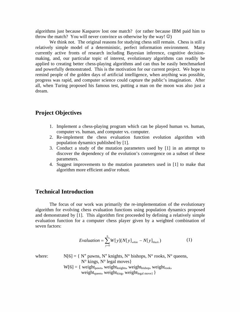
Technical Introduction The focus of our work was primarily the re-implementation of the evolutionary algorithm for evolving chess evaluation functions using population dynamics proposed and demonstrated by [1]. This algorithm first proceeded by defining a relatively simple evaluation function for a computer chess player given by a weighted combination of seven factors:

∑=

−=6

0

)][][]([y

blackwhite yNyNyWEvaluation (1)

where: N[6] = { N° pawns, N° knights, N° bishops, N° rooks, N° queens,

N° kings, N° legal moves} W[6] = { weightpawn, weightknights, weightbishop, weightrook, weightqueen, weightking, weightlegal move} }

The parameter to be evolved is, of course, the weight vector W. The original algorithm then created an initial population of 50 alpha-beta chess-players each with the above evaluation function and its own random W vector. The weights were initially uniformly selected from the range [0,12]. The evolution then began by allowing chess players to compete against one another in a particular fashion which ensured that stronger players were allowed to play more often than weak ones. Each match consisted of two games with players taking turns as white or black. More games were not required since the algorithms are entirely deterministic and the outcome would therefore never change. After each match, if there was a clear winner, the loser was removed from the population. In its place, a mutated copy of the winner would be created. The winner might also be mutated in place. Mutations took place by adding or subtracting a scaled number onto each element of a population member’s weight vector. Thus:

( )( ))()()( 5.0)1..0( yyy RRNDVV σ××−+= ν∈∀y

Player wins both games: Expel loser, duplicate winner and mutate one copy by R = 0 and the other copy by R = 2.

Player wins one game and draws the other: Expel loser, duplicate winner and mutate one copy by R = .2 and the other copy R = 1.

Players draw: Both players are retained and mutated by R = .5. The astute reader will immediately note that the R values above seem rather ad hoc, and indeed Kendall and Whitwell note that the R values were “selected based on initial testing” and not by any theoretical or rigorous means [1]. It was therefore our purpose in this project to empirically discover evidence for or against the mutation parameter choices chosen by Kendall and Whitwell. Our empirical experiments demonstrate that in fact this evolutionary algorithm is extremely sensitive to the mutation parameters chosen. If the parameters are chosen too large, the algorithm may frequently become unstable and never converge to a single value. If the parameters are chosen too small, the algorithm may converge quickly, but to a value that is less than optimal. In the middle range, the parameters may be tuned to increase or decrease the convergence rate of the algorithm toward the optimal solution. However, if no knowledge of the correct optimal solution exists, we show that evolutionary algorithms may in fact be very difficult or impossible to properly tune.

Previous Work In choosing to study the effects of mutation parameters on evolution convergence, we first needed to research the literature and see what studies, if any, had been conducted along these same lines. The number of papers on general evolutionary algorithms is astounding [5][7][8], it having become a veritable buzzword in the late nineties. However, most of these papers focus on solitary attempts to create an evolutionary

algorithm for a particular field. Many fewer of the papers in the literature are actually detailed theoretical analyses of how an evolutionary algorithm should be created [6][9] and practically none provide detailed evidence as to why they chose their mutation parameters as they did. The reason for this gaping lack can probably be best summed up by a passage from [5]: “Probably the tuning of the GA [Genetic Algorithm] parameters are likely to accelerate the convergence [of the evolution]. Unfortunately, the tuning is rather difficult, since each GA run requires excessive computational time.” It seems that authors have been generally much too concerned with turning out a paper containing a neat application in as short a time as possible and much less eager to invest the admittedly exorbitant amount of time and computational resources required to investigate this question. After this rather dismaying survey of the literature, we decided that our investigation would therefore be quite beneficial to the field. Unfortunately, we too were limited by the computational time requirements requisite of this ambitious undertaking.

The Chess-Playing Algorithm In Detail

Alpha-Beta Search as Branch and Bound: The Alpha-Beta search which is the core of the adversarial search in cognitive game theory can be seen as two simple Branch and Bound algorithms in parallel. Branch and Bound is used to find the minimum assignment to a set of variables given a list of soft constraints (all with positive penalty). Similarly Alpha-Beta is used to find the branch in the game tree which corresponds to the optimum move for the computer applying the minimax rule and using the chess rules as constraints. The two algorithms are obviously quiet different, but the pruning rule is the same.

In Branch and Bound we can prune a subtree if the value of the current assignment at the root of the subtree is already greater than the best solution found so far for the complete set of variables. We can apply such a method because the constraints only have a deleterious impact on the value of the assignment (there is no negative penalty). Therefore, when considering a subset of variables, we know that if we already found a better solution using the complete set of variables, there is no reason to continue searching the subtree. At best the new constraints will be satisfied with a cost of zero but the final value will still be greater than the intermediary value and worse than the optimum.

At first glance, it is not obvious how this relates to Alpha-Beta since the minimax algorithm uses positive as well as negative penalties, depending on which player is playing, and there is no constraint defined at a given node. First with Alpha-Beta we can only evaluate the nodes starting from the leaves and back up the values in the search tree. For each MIN node, we return the minimum of the value of the children and for each MAX node we return the maximum of the values of the children. From this guideline we can easily define the Alpha-Beta pruning rule. Imagine that for a given MAX node we found a child worth 10. If elsewhere in the subtree starting from this node we find another MAX node with a worse value of 6, there is no need to continue expanding the siblings of this sub-node. We can then prune the parent of this node. Indeed, whatever the values of the siblings are, the parent node (which is a MIN node) will always be able to

return this 6 to the initial node and therefore the MAX node root of the subtree will never choose this move since it can have a 10 with another move.

In the alpha-beta procedure we define two parameters from which we'll be able to prune the game tree according to the Branch and Bound procedure:

• Alpha (highest values seen so far on max level) • Beta (lowest value seen so far on min level).

Alpha and Beta are local to any subtree. The idea of the Alpha-Beta pruning is that if we find a value which is smaller than the current Alpha (for MAX) or greater than the current Beta (for MIN), we don't have to expand any other sibling since we already found a better solution elsewhere. Hence we can see the Alpha-Beta search as two Branch and Bounds search in parallel, one for each player MIN and MAX.

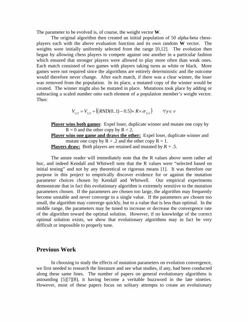
The MIN level is exactly the same as a normal Branch and Bound: we want to minimize the value of the node which is exactly the same as minimizing the value of the tuple assignment for B&B. As far as pruning, we don't expand any other sibling for a node whose evaluation function is greater than Beta (the minimum board evaluation seen so far on the subtree restricted to MIN nodes). Again this is the same as pruning a node if the value of the given assignment of the subset of variable is greater than the best solution seen so far.

Figure 1: Example of Beta-pruning (exactly similar to B&B)

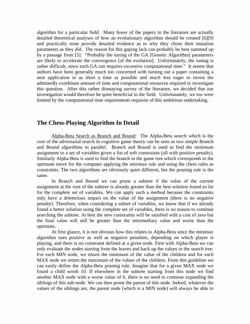
The MAX level is the inverse of the normal Branch and Bound since we want to maximize the value of the nodes It can be seen as a B&B. But the idea is still the same and the procedure similar. As far as pruning, for a MAX node, want don't expand any other siblings for a node whose value is smaller than Alpha, the maximum board evaluation seen so far on the MAX levels of the subtree.

Figure 2: Example of Alpha-pruning (inverse of B&B)

3 1 -5

3

4

≥ 4

2Min

Beta not defined Beta = 3 Beta = 3

2Max

1 0 2

3 1 5

3

1Max

Alpha not defined Alpha = 3 Alpha = 10

10

1

≤ 2 Min

22 1

Finally, the Alpha-Beta search can be seen as two B&B searches in parallel, one for the MAX nodes and one for the MIN nodes. To make the search more efficient, only the “interesting” nodes are searched, and similarly to B&B, we prune all the nodes that cannot possibly influence the final decision. The pruning rule is however slightly different because whereas for B&B we have a value for a node before searching any child (just by evaluating the set of constraints defined on the current tuple) for Alpha-Beta we have to search down to the maximum depth of the search in order to apply the evaluation function and return a value for the node. Therefore, instead of simply pruning the node, in Alpha-Beta the gain is to cancel the search of the other siblings. It can be compared to pruning the parent node (MAX node just above for MIN or MIN node just above for MAX). Adaptations to Alpha-Beta: The alpha-beta algorithm alone is a very powerful tool for evaluating possible moves in a game tree. However, for many applications it still evaluates more positions than is necessary or feasible if a deep-searching algorithm is required. As such, the literature has proposed numerous improvements to the basic search algorithm over the years. The three improvements implemented by Kendall and Whitwell, and later by us, are discussed below.

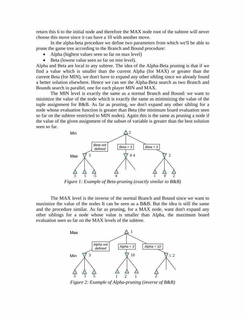
Transposition Tables: In many cases, a combination of two or more moves may be performed in different orderings but arrive at the same final board state. In such a case, Figure 3 illustrates that the naïve alpha-beta algorithm will reach this same board state, not recognize that it has seen the position before, and be forced to continue searching deeper in the tree even though it has already searched this subtree before. If the search is able to instead save to memory a table of board positions previously explored and evaluated, the wasted computation of expanding the subtree multiple times can be avoided.

Figure 3: (a) Naïve alpha-beta. The search assigns a value of 35 to the square node after searching the entire subtree. When the search again sees

square, it must re-explore the subtree. (b)

Transposition tables enabled. The search

stores the value 35 for square node in

memory. When it again sees square node,

it can immediately assign its value with no

further search.

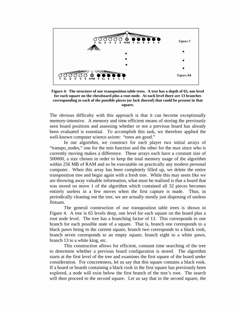
Figure 4: The structure of our transposition table trees. A tree has a depth of 65, one level

for each square on the chessboard plus a root node. At each level there are 13 branches corresponding to each of the possible pieces (or lack thereof) that could be present in that

square. The obvious difficulty with this approach is that it can become exceptionally memory-intensive. A memory and time efficient means of storing the previously seen board positions and assessing whether or not a previous board has already been evaluated is essential. To accomplish this task, we therefore applied the well-known computer science axiom: “trees are good.”

In our algorithm, we construct for each player two initial arrays of “transpo_nodes,” one for the min function and the other for the max since who is currently moving makes a difference. These arrays each have a constant size of 500000, a size chosen in order to keep the total memory usage of the algorithm within 256 MB of RAM and so be executable on practically any modern personal computer. When this array has been completely filled up, we delete the entire transposition tree and begin again with a fresh tree. While this may seem like we are throwing away valuable information, what must be realized is that a board that was stored on move 1 of the algorithm which contained all 32 pieces becomes entirely useless in a few moves when the first capture is made. Thus, in periodically cleaning out the tree, we are actually mostly just disposing of useless flotsam.

The general construction of our transposition table trees is shown in Figure 4. A tree is 65 levels deep, one level for each square on the board plus a root node level. The tree has a branching factor of 13. This corresponds to one branch for each possible state of a square. That is, branch one corresponds to a black pawn being in the current square, branch two corresponds to a black rook, branch seven corresponds to an empty square, branch eight to a white pawn, branch 13 to a white king, etc.

This construction allows for efficient, constant time searching of the tree to determine whether a previous board configuration is stored. The algorithm starts at the first level of the tree and examines the first square of the board under consideration. For concreteness, let us say that this square contains a black rook. If a board or boards containing a black rook in the first square has previously been explored, a node will exist below the first branch of the tree’s root. The search will then proceed to the second square. Let us say that in the second square, the

current board contains a white king. If the transposition table had already seen a board that contained a black rook in square 1 and a white king in square 2, a child node would exist beneath the thirteenth branch of the current node. In this way, the search can continue down the tree, taking at most 64 steps until it has determined that all of the squares of the current board do or do not match a board previously seen. If the board does match, the value of the previously explored subtree for the given board is returned. If the board does not match after some depth, then the necessary nodes are added to the transposition tree to signify that such a board has now been seen and the alpha-beta search is forced to continue.

However one has to be cautious when applying this process because we don’t want to limit the search depth by applying the transposition tables. When checking if a board configuration has already been seen in the table, it may be that it has been seen but at a high depth in the search. Then the value associated in the table may correspond to a search only one or two plies ahead from this board configuration. In such a case if we find a board that matches this board in the table we don’t want to return the value in the table if the planned depth of the search for the new board is greater than the search of the board in the table. To solve this problem, we recorded in the transposition tables the depth of the search that led to the value of the boards stored. Then a board that matches a board in the table is only pruned if the planned search depth is smaller (or equal) than the one recorded is the table.

Our approach to transposition trees was able to achieve a constant memory usage, a constant search time for previously seen boards, and a constant time update to the table given new information. We are quite proud of that approach which we developed without any help from the literature.

Quiescent Search: The second improvement on simple alpha-beta search that we implemented for our chess player is known as quiescent search. The principle behind this search is an attempt to eliminate what is known as the search horizon. The weakness of naive evaluation functions – like the one used in the Kendall and Whitwell paper and therefore in our chess player – is that they only evaluate static board configurations. They cannot foresee if the next move is a capture that will totally change the “value” of the board. This is especially true if we stop the search at a fixed depth. The idea of “quiescent search” is to use a variable search depth and only apply the evaluation function to stable board configurations. Imagine that we have a board in which black’s queen and white’s pawn can attack the same square which is currently occupied by white’s bishop. In this position, black’s best next move would be to capture white’s bishop with his queen. This move would make our heuristic evaluation function favor black if we stopped at only one level deeper. However, if we search two moves deep, we will see that black’s queen having taken white’s bishop would in turn be captured by white’s pawn. The bishop capture is in fact then a very bad move for black. However, black is simply unable to see past its depth horizon of one, and so does not realize that it has moved its queen into jeopardy. This problem stems from the

fact that our heuristic function does not adequately take into account the true future strategic value of a current board, but is rather only a rough estimate of this position based purely on the events which have happened in the past. One solution to this problem then would be to incorporate more future information into one’s evaluation function. This approach has been avidly pursued [10][12]. For our present purposes, however, the structure of our evaluation function has been presupposed as similar to Kendall and Whitwell’s, and we must therefore find another method for dealing with this finite horizon search issue. The quiescent search methodology is a partial solution to this problem. Basically, when the alpha-beta search reaches its “maximum depth” it does not immediately cease searching in all cases. It first examines the current board position to see if the board configuration at the next level is relatively stable. In our algorithm, this is done by querying whether or not there are any capture or promotion moves available at the next level of the search tree. If the alpha-beta search finds that the board configuration is not stable at this level, then it proceeds to search an extra level of depth. As long as there are more capture moves available, the search will continue, theoretically indefinitely. This would ensure that when the search has reached a leaf, the heuristic function at the leaf is relatively stable and therefore is an adequate representation of the current board position. Unfortunately, in a practical sense, we cannot allow the alpha-beta to continue indefinitely searching for all captures as that would require far too much computational time. Instead, we allow the quiescent search to proceed to a level between two and three times as deep as the initial “maximum” depth level. If in the intervening levels a node is found which does not have any available captures in the next level, the search is halted at this level. Otherwise, when the search has reached three times the maximum depth, the search is halted regardless. Obviously, as was mentioned, this is only a partial solution to the problem of search horizon. It seems we have simply exchanged one horizon for a slightly deeper horizon. This is more or less the case. However, quiescent search is a logical attempt, using a practical amount of computational resources, to continue down search paths until a stable, representative evaluation function can be found. If this is not possible within a reasonable amount of time, we simply must be satisfied with the dangerous approximation we are making and realize that just as humans are fallible, so too will be our search algorithm.

Heuristic Move-Ordering: The efficiency of the alpha-beta search is

highly dependent upon the order in which board positions are evaluated. If the search is able to quickly narrow its pruning window and if the extreme values at each leaf are evaluated first, it will be able to efficiently rule out positions which must necessarily obtain values outside of the search window.

To this end, the next move to consider in chess should be ordered to provide the maximum possible likelihood of cut-off, meaning it should be the most extreme value possible. Since capture or promotion moves alter the evaluation function of the board most profoundly, it stands to reason that considering these moves first will lead to better ordering of leaf nodes. [3]

Our algorithm does exactly this. When considering which branch to explore first in the min-max search tree, we first compile a list of all the possible capture or promotion moves available from the current position. Each move in this list is then scored by the change it will make to the evaluation function, meaning in our case that the score is the absolute value of the captured piece in terms of the current weight vector being evolved (or the difference between the queen and the pawn value for a promotion). That is, if the weight vector for the current player values a queen at 900, then the value assigned to a move capturing the queen will be 900. The moves with the highest scores are then evaluated first followed by the remaining lower score capture moves. Once all capture or promotion moves have been searched, the regular moves are next considered. These are not ordered in any very significant manner, except that we tend to consider moves by more powerful pieces first, expecting them to have the most impact on the game.

Benchmarking of Alpha-Beta Improvements: In the literature, these

alpha-beta improvement techniques are often proposed and used to increase search performance. However, it is difficult to find any quantitative analysis of just how effective these improvements are and how much benefit in decreased computation is gained by their usage. As such, we conducted our own miniature empirical study of the effects of alpha-beta and each of its three improvements on the number of nodes searched and the time required to perform a search using our original checkers algorithm as a testbed. Table 1 presents the results of these trials for various depths of search. Note that the columns titled quiescent search and transposition tables represent the results for a mini-max search without alpha-beta prunning. This was done to further separate the variables and attain a better understanding of exactly how large an effect each improvement had on the entire search tree. Note the significant benefit gained in number of nodes searched when alpha-beta was used alone or with move ordering, as well as the significant decrease in computation associated with the use of either variable search depth (quiescent search) or transposition tables, especially at higher depths. It might be interesting to note that the column corresponding to “quiescent search” is a variable-depth minimax search conducted between a depth equal to one half of the indicated depth and the indicated depth. This is approximately as efficient as a fixed depth search to the indicated depth because for a given board it will return a more precise evaluation of the board applied to a shallower (sometimes but not always) but more stable board or the same evaluation function as the basic minimax search.

We did the empirical study of the improvements using our checkers algorithm because we used checkers to develop our search algorithm and then we just adapted it for chess. Anyhow the results should be similar for the chess algorithm. Since the branching factor in the game tree is greater for chess than for checkers, it might be that the Alpha-Beta pruning is relatively more efficient for chess than the other improvements. And because there are a lot more possible moves in chess than in checkers, it might also be that the quiescent search improvement is a little bit less efficient relatively.

Depth Minimax Alpha-

Beta + Move ordering

Quiesc. search

Transpo. tables

4 3308 278 271 2078 2237 6 217537 5026 3204 41219 50688

Number of

nodes 8 15237252 129183 36753 649760 859184 4 0 0 0 0 0 6 3 0 0 0 1

Search time (sec.) 8 201 1 0 9 12

Table 1: The results of benchmarking alpha-beta and its improvements.

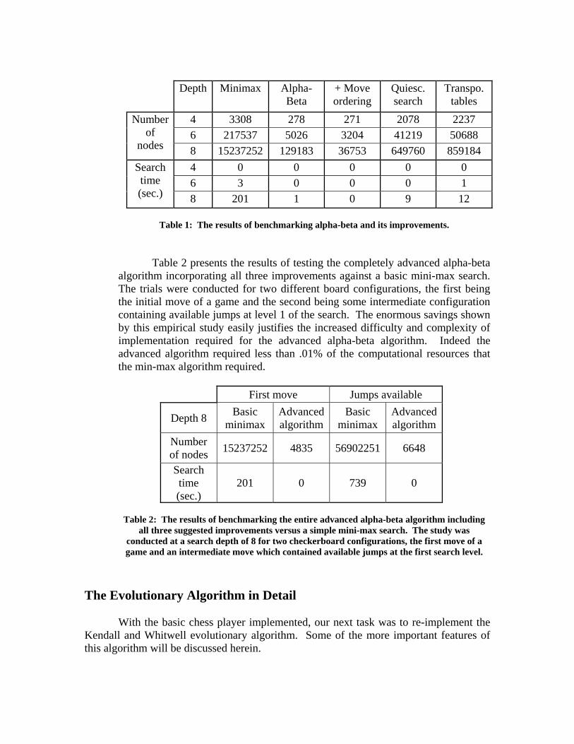
Table 2 presents the results of testing the completely advanced alpha-beta algorithm incorporating all three improvements against a basic mini-max search. The trials were conducted for two different board configurations, the first being the initial move of a game and the second being some intermediate configuration containing available jumps at level 1 of the search. The enormous savings shown by this empirical study easily justifies the increased difficulty and complexity of implementation required for the advanced alpha-beta algorithm. Indeed the advanced algorithm required less than .01% of the computational resources that the min-max algorithm required.

First move Jumps available

Depth 8 Basic minimax

Advanced algorithm

Basic minimax

Advanced algorithm

Number of nodes 15237252 4835 56902251 6648

Search time (sec.)

201 0 739 0

Table 2: The results of benchmarking the entire advanced alpha-beta algorithm including

all three suggested improvements versus a simple mini-max search. The study was conducted at a search depth of 8 for two checkerboard configurations, the first move of a game and an intermediate move which contained available jumps at the first search level.

The Evolutionary Algorithm in Detail

With the basic chess player implemented, our next task was to re-implement the Kendall and Whitwell evolutionary algorithm. Some of the more important features of this algorithm will be discussed herein.

Selection Process: Since the chess players are entirely deterministic, competition could be performed by two players playing just two games against one another, once as black and once as white. The authors proposed a novel sequence of player choice which they proved would allow the best player in the population (if it existed) to end each generation in the final position, viewing the entire population as a vector. Figure 5, courtesy of [1], details this process. Basically, the strategy is to have µ−1 matches per generation where µ is the size of the population. For the ith match, the first player is chosen to be the player at position i within the population. The second player, j, is chosen from the tail of the population vector. That is:

µ≤≤+ ji 1

In this way, as Figure 5 shows, the most powerful evaluation function currently in the vector should be involved in many matches and thus propagate quickly throughout the entire population.

Mutation Process: optimum player in evolve at the sameconvergence is actuthree main reasons:

• First, the mewhich, even small search

The goal of the evolution procedure is to converge toward the a 6-dimensional space (6 parameters of the evaluation function to time) starting from a discrete random population of seeds. This ally a very complicated problem from a mathematical standpoint for

tric used for to determine mutation is the outcome of a chess game if deterministic, is not a perfect evaluation of the player’s quality. At depths, a “better” player can have a “better” evaluation function but

still head toward a “beyond-the-horizon” dead-end that eventually leads to the opponent’s victory. We can get rid of this problem – at least partially – by increasing the depth of the search. Indeed if the horizon is farther away there will be less chance to head toward a dead-end because there will be more possibilities to escape. With higher search depths, the outcomes of the games between the players should be more “fair”. Unfortunately, due to the severe time and computational constraints of this project, we could only experiment at reasonably shallow search depths, and consequently we perform our evolutions with a variable search depth between 2 and 5. This is obviously not enough to completely avoid the horizon effect, and this may have been one reason that our convergence results appear slower than those reported by Kendall and Whitwell. It may also account for the difference in the optimal values for evaluation function parameters that we eventually obtained; Kendall and Whitwell did not completely define the parameters of their quiescent search and so attempting to match their results completely proved impossible. Despite these difficulties, the procedure should still eventually converge toward the set of parameters which is optimal for the particular search depth used.

• A second difficulty is due to the high number of parameters being evolved at the same time: the higher the dimension of the space the more challenging the convergence. When a player loses a game, we mutate all the weights in that player with the same coefficient though the defeat was maybe due to only one of them. Hence even if the player was converged in several but not all dimensions (say rook, knight and queen) we just throw it away because of the other parameters (say bishop and legal moves). In our study this is especially a problem with the weight associated with the number of legal moves. While the other weights are generally only multiplied by one or two, corresponding to the number of pieces of that type remaining on the board, the legal moves weight is often multiplied by 20 or 30. If this weight is of the same order of magnitude as the other weights, one can easily see that it will completely swamp any differences between other dimensions. Therefore if this weight has a large value but all other weights have been optimized, the player may still very well lose its matches.

• The last difficulty is less important than the first two and only appears after a certain time in the convergence procedure. It is another consequence of the “game outcome” metric used. When all the population members are similar to one another, the evaluation functions of the different players might not be different enough to differentiate the players. In this case most of the games will be draws. This problem prevents the population from ever completely converging. After the evolution procedure has finished, therefore, we take the average of the final population to be the optimum player.

For these three reasons, the mutation procedure has to be thought out carefully in

order for the evolution to succeed. If the mutation parameters are not appropriate, the parameters population will not necessarily converge toward the optimum player or may even diverge. The mutation procedure is actually defined from the metric output. There

are four possible outcomes for a chess match consisting of two games: each player playing as black and white):

• One of the player wins both games • One player wins one game and the other game is a draw • The two games are draws • Each player wins one game

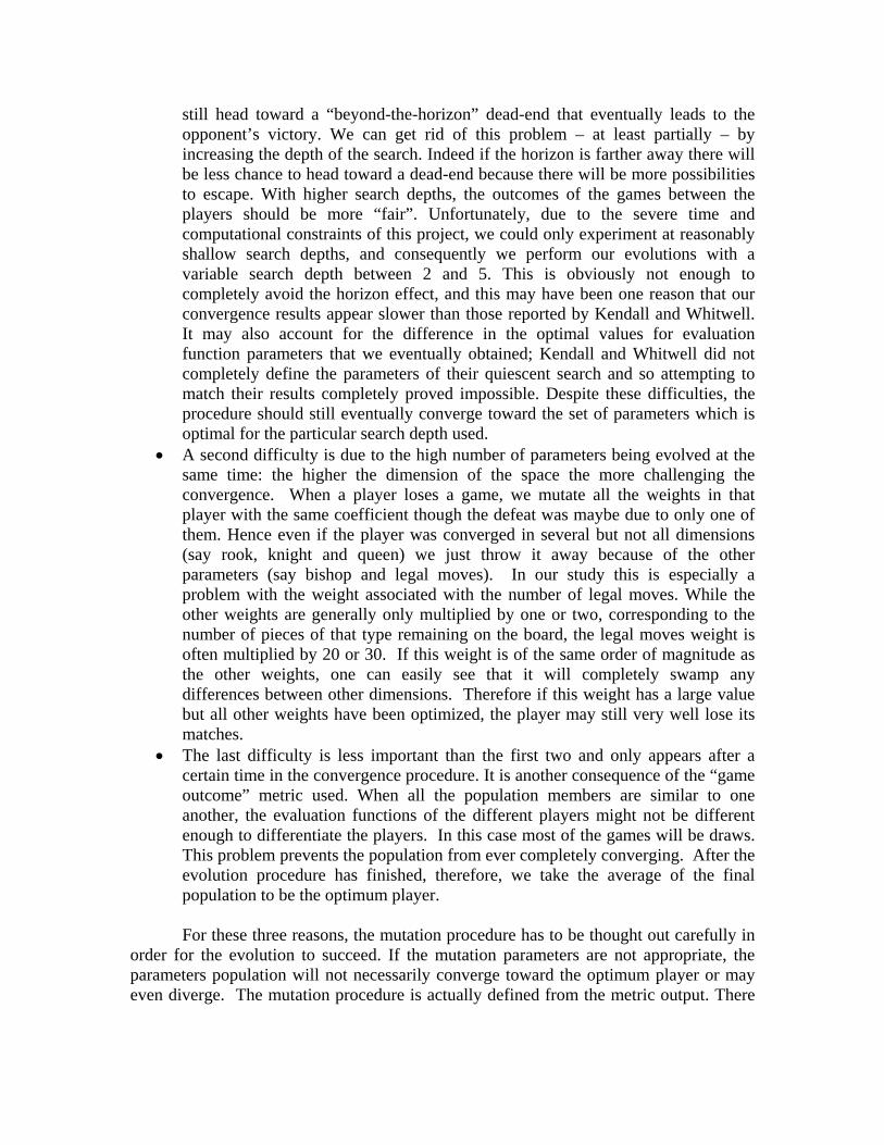
The two last cases are assumed to be equivalent in our procedure. For each situation we have to define a mutation procedure for the two players. In the paper that describes the evolution procedure we applied [1], they chose to remove the loser (if any) from the population replacing it by a clone of the winner. Then they mutated each weight of the two players according to the equation:

( )( ))()()( 5.0)1..0( yyy RRNDVV σ××−+=

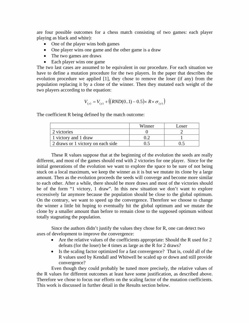
The coefficient R being defined by the match outcome:

Winner Loser 2 victories 0 2 1 victory and 1 draw 0.2 1 2 draws or 1 victory on each side 0.5 0.5

These R values suppose that at the beginning of the evolution the seeds are really

different, and most of the games should end with 2 victories for one player. Since for the initial generations of the evolution we want to explore the space to be sure of not being stuck on a local maximum, we keep the winner as it is but we mutate its clone by a large amount. Then as the evolution proceeds the seeds will converge and become more similar to each other. After a while, there should be more draws and most of the victories should be of the form “1 victory, 1 draw”. In this new situation we don’t want to explore excessively far anymore because the population should be close to the global optimum. On the contrary, we want to speed up the convergence. Therefore we choose to change the winner a little bit hoping to eventually hit the global optimum and we mutate the clone by a smaller amount than before to remain close to the supposed optimum without totally stagnating the population.

Since the authors didn’t justify the values they chose for R, one can detect two

axes of development to improve the convergence: • Are the relative values of the coefficients appropriate: Should the R used for 2

defeats (for the loser) be 4 times as large as the R for 2 draws? • Is the scaling factor optimized for a fast convergence? That is, could all of the

R values used by Kendall and Whitwell be scaled up or down and still provide convergence?

Even though they could probably be tuned more precisely, the relative values of the R values for different outcomes at least have some justification, as described above. Therefore we chose to focus our efforts on the scaling factor of the mutation coefficients. This work is discussed in further detail in the Results section below.

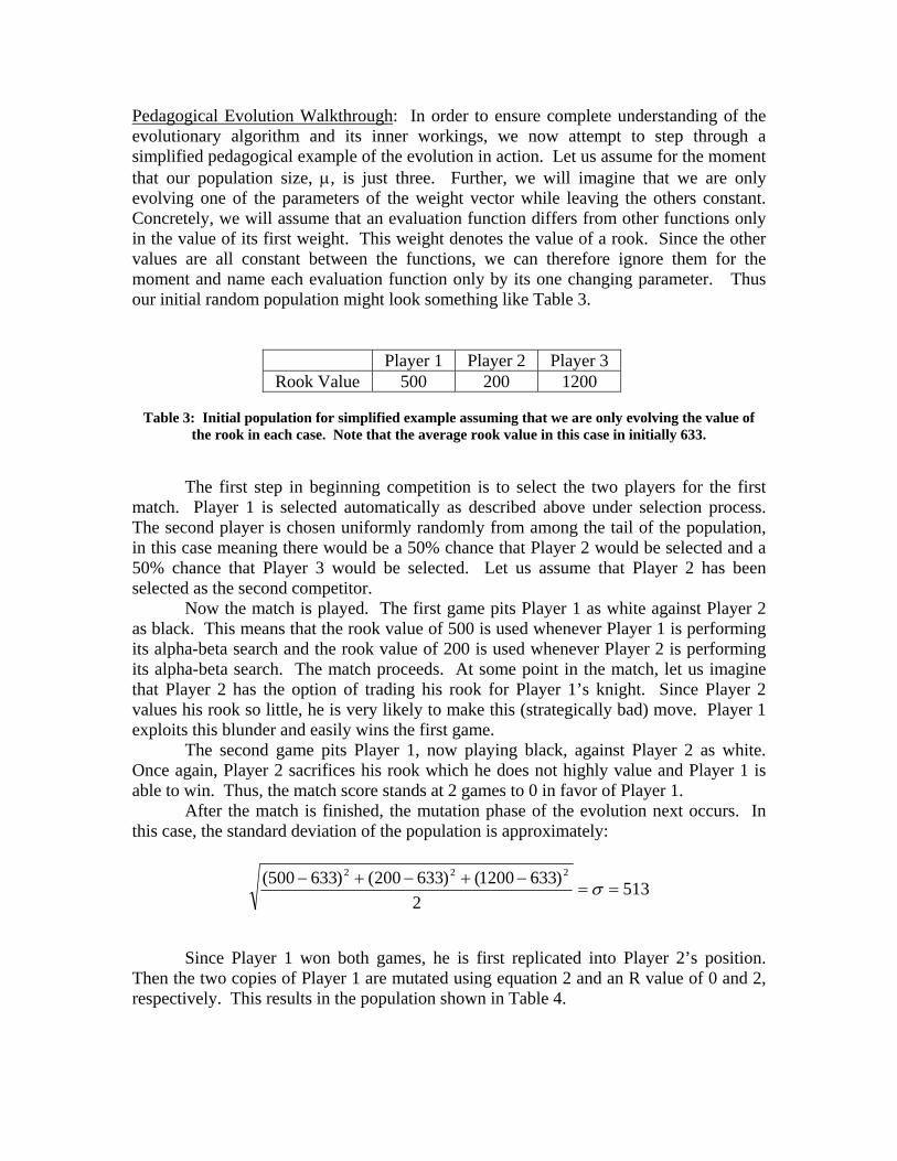
Pedagogical Evolution Walkthrough: In order to ensure complete understanding of the evolutionary algorithm and its inner workings, we now attempt to step through a simplified pedagogical example of the evolution in action. Let us assume for the moment that our population size, µ, is just three. Further, we will imagine that we are only evolving one of the parameters of the weight vector while leaving the others constant. Concretely, we will assume that an evaluation function differs from other functions only in the value of its first weight. This weight denotes the value of a rook. Since the other values are all constant between the functions, we can therefore ignore them for the moment and name each evaluation function only by its one changing parameter. Thus our initial random population might look something like Table 3.

Player 1 Player 2 Player 3 Rook Value 500 200 1200

Table 3: Initial population for simplified example assuming that we are only evolving the value of

the rook in each case. Note that the average rook value in this case in initially 633. The first step in beginning competition is to select the two players for the first match. Player 1 is selected automatically as described above under selection process. The second player is chosen uniformly randomly from among the tail of the population, in this case meaning there would be a 50% chance that Player 2 would be selected and a 50% chance that Player 3 would be selected. Let us assume that Player 2 has been selected as the second competitor. Now the match is played. The first game pits Player 1 as white against Player 2 as black. This means that the rook value of 500 is used whenever Player 1 is performing its alpha-beta search and the rook value of 200 is used whenever Player 2 is performing its alpha-beta search. The match proceeds. At some point in the match, let us imagine that Player 2 has the option of trading his rook for Player 1’s knight. Since Player 2 values his rook so little, he is very likely to make this (strategically bad) move. Player 1 exploits this blunder and easily wins the first game. The second game pits Player 1, now playing black, against Player 2 as white. Once again, Player 2 sacrifices his rook which he does not highly value and Player 1 is able to win. Thus, the match score stands at 2 games to 0 in favor of Player 1. After the match is finished, the mutation phase of the evolution next occurs. In this case, the standard deviation of the population is approximately:

5132

)6331200()633200()633500( 222

==−+−+− σ

Since Player 1 won both games, he is first replicated into Player 2’s position. Then the two copies of Player 1 are mutated using equation 2 and an R value of 0 and 2, respectively. This results in the population shown in Table 4.

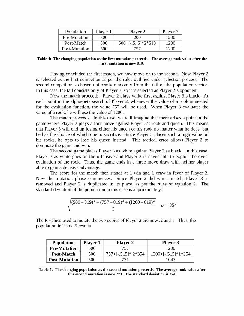
Population Player 1 Player 2 Player 3 Pre-Mutation 500 200 1200 Post-Match 500 500+[-.5,.5]*2*513 1200

Post-Mutation 500 757 1200

Table 4: The changing population as the first mutation proceeds. The average rook value after the first mutation is now 819.

Having concluded the first match, we now move on to the second. Now Player 2 is selected as the first competitor as per the rules outlined under selection process. The second competitor is chosen uniformly randomly from the tail of the population vector. In this case, the tail consists only of Player 3, so it is selected as Player 2’s opponent. Now the match proceeds. Player 2 plays white first against Player 3’s black. At each point in the alpha-beta search of Player 2, whenever the value of a rook is needed for the evaluation function, the value 757 will be used. When Player 3 evaluates the value of a rook, he will use the value of 1200. The match proceeds. In this case, we will imagine that there arises a point in the game where Player 2 plays a fork move against Player 3’s rook and queen. This means that Player 3 will end up losing either his queen or his rook no matter what he does, but he has the choice of which one to sacrifice. Since Player 3 places such a high value on his rooks, he opts to lose his queen instead. This tactical error allows Player 2 to dominate the game and win. The second game places Player 3 as white against Player 2 as black. In this case, Player 3 as white goes on the offensive and Player 2 is never able to exploit the over-evaluation of the rook. Thus, the game ends in a three move draw with neither player able to gain a decisive advantage. The score for the match then stands at 1 win and 1 draw in favor of Player 2. Now the mutation phase commences. Since Player 2 did win a match, Player 3 is removed and Player 2 is duplicated in its place, as per the rules of equation 2. The standard deviation of the population in this case is approximately:

3542

)8191200()819757()819500( 222

==−+−+− σ

The R values used to mutate the two copies of Player 2 are now .2 and 1. Thus, the population in Table 5 results.

Population Player 1 Player 2 Player 3 Pre-Mutation 500 757 1200 Post-Match 500 757+[-.5,.5]*.2*354 1200+[-.5,.5]*1*354

Post-Mutation 500 771 1047

Table 5: The changing population as the second mutation proceeds. The average rook value after this second mutation is now 773. The standard deviation is 274.

So after just two mutations and one generation, we have taken a population that started with standard deviation of 513 and nearly halved that value to just 274. The population has already begun to converge toward some final value. The evolution would hereafter proceed by first inverting the population vector, meaning in this case that Player 3 would be placed into the first position and Player 1 would be placed into the third position. Then generations similar to the one just stepped through would occur. The evolution would proceed either for some set number of generations, some predetermined amount of real-world time had elapsed, or until some small value had been reached for the standard deviation indicating that no further convergence was necessary for the population. In this way, an initially random population of players can be competed, mutated, and evolved to discover a much more optimal population of players without the need for expert domain specific knowledge to tune the various relative weights.

Results of Experiments Comparison to Existing Algorithm Our first goal was to implement Kendall and Whitwell’s algorithm and to reproduce as closely as possible the results they published in their paper. Unfortunately, we found this task to be nearly impossible due to a number of unidentified parameters of their algorithm. The first of these parameters is what the authors described as “a small fixed bonus . . . given for control of the center squares and advanced pawns with promotion potential.” [1] The value of this small fixed bonus was not, however, explicitly stated in the paper. As such, we opted to select a value of zero for this bonus, feeling that in this way we would know which direction the data should be affected. That is, by choosing not to include the bonus, we realized that pawns would certainly be worth less than in Kendall and Whitwell’s results because the computer would not be trying to hold onto them in order to retain the promotion bonus. If we had guessed a value for this bonus, we could have guessed too high or too low and would not have known in which direction our results should have been affected. As such, we can now expect with confidence that pawns in our algorithm will be worth some amount less than the authors found them to be, or in other words that the other pieces will have relatively higher values than in the Kendall and Whitwell case. Similarly, the bonus for center square control was set to zero for the same reason. By choosing zero, we know that we have guessed too low and could adjust our data appropriately if necessary. A second source of possible difference between our algorithms was the lack of clear definition of the quiescent search method employed by the authors. They simply stated that “quiescence was used to selectively extend the search tree to avoid noisy board positions where material exchanges may influence the resultant evaluation quality” and cited the work by Bowden which first introduced the concept of quiescent search. [13] This left us wondering how deep would be deep enough. As has been previously noted, the depth of the search can have a profound effect on the optimal evaluation function as

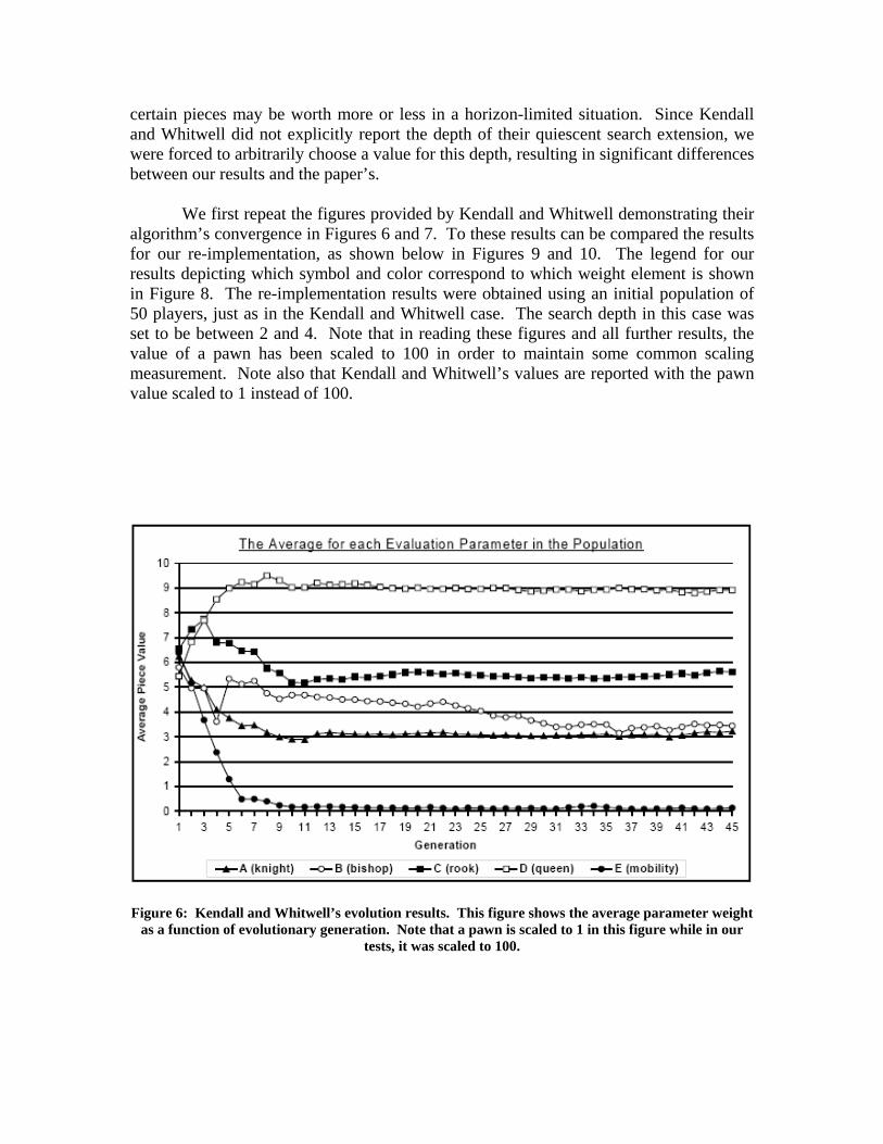
certain pieces may be worth more or less in a horizon-limited situation. Since Kendall and Whitwell did not explicitly report the depth of their quiescent search extension, we were forced to arbitrarily choose a value for this depth, resulting in significant differences between our results and the paper’s. We first repeat the figures provided by Kendall and Whitwell demonstrating their algorithm’s convergence in Figures 6 and 7. To these results can be compared the results for our re-implementation, as shown below in Figures 9 and 10. The legend for our results depicting which symbol and color correspond to which weight element is shown in Figure 8. The re-implementation results were obtained using an initial population of 50 players, just as in the Kendall and Whitwell case. The search depth in this case was set to be between 2 and 4. Note that in reading these figures and all further results, the value of a pawn has been scaled to 100 in order to maintain some common scaling measurement. Note also that Kendall and Whitwell’s values are reported with the pawn value scaled to 1 instead of 100.

Figure 6: Kendall and Whitwell’s evolution results. This figure shows the average parameter weight

as a function of evolutionary generation. Note that a pawn is scaled to 1 in this figure while in our tests, it was scaled to 100.

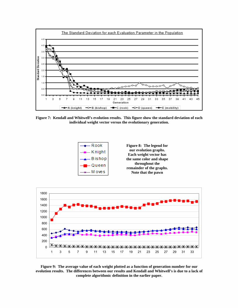
Figure 7: Kendall and Whitwell’s evolution results. This figure show the standard deviation of each individual weight vector versus the evolutionary generation.

0

200

400

600

800

1000

1200

1400

1600

1800

1 3 5 7 9 11 13 15 17

Figure 9: The average value of each weight plotted

evolution results. The differences between our resultscomplete algorithmic definiti

Figure 8: The legend for our evolution graphs.

Each weight vector has the same color and shape

throughout the remainder of the graphs.

Note that the pawn

19 21 23 25 27 29 31 33

as a function of generation number for our and Kendall and Whitwell’s is due to a lack of

on in the earlier paper.

0

100

200

300

400

500

600

700

1 3 5 7 9 11 13 15 17 19 21 23 25 27 29 31 33

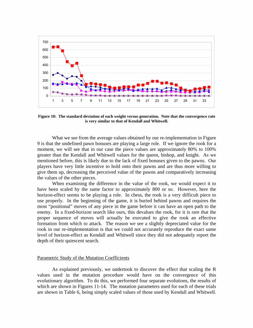
Figure 10: The standard deviation of each weight versus generation. Note that the convergence rate is very similar to that of Kendall and Whitwell.

What we see from the average values obtained by our re-implementation in Figure 9 is that the undefined pawn bonuses are playing a large role. If we ignore the rook for a moment, we will see that in our case the piece values are approximately 80% to 100% greater than the Kendall and Whitwell values for the queen, bishop, and knight. As we mentioned before, this is likely due to the lack of fixed bonuses given to the pawns. Our players have very little incentive to hold onto their pawns and are thus more willing to give them up, decreasing the perceived value of the pawns and comparatively increasing the values of the other pieces. When examining the difference in the value of the rook, we would expect it to have been scaled by the same factor to approximately 800 or so. However, here the horizon-effect seems to be playing a role. In chess, the rook is a very difficult piece to use properly. In the beginning of the game, it is buried behind pawns and requires the most “positional” moves of any piece in the game before it can have an open path to the enemy. In a fixed-horizon search like ours, this devalues the rook, for it is rare that the proper sequence of moves will actually be executed to give the rook an effective formation from which to attack. The reason we see a slightly depreciated value for the rook in our re-implementation is that we could not accurately reproduce the exact same level of horizon-effect as Kendall and Whitwell since they did not adequately report the depth of their quiescent search. Parametric Study of the Mutation Coefficients As explained previously, we undertook to discover the effect that scaling the R values used in the mutation procedure would have on the convergence of this evolutionary algorithm. To do this, we performed four separate evolutions, the results of which are shown in Figures 11-14. The mutation parameters used for each of these trials are shown in Table 6, being simply scaled values of those used by Kendall and Whitwell.

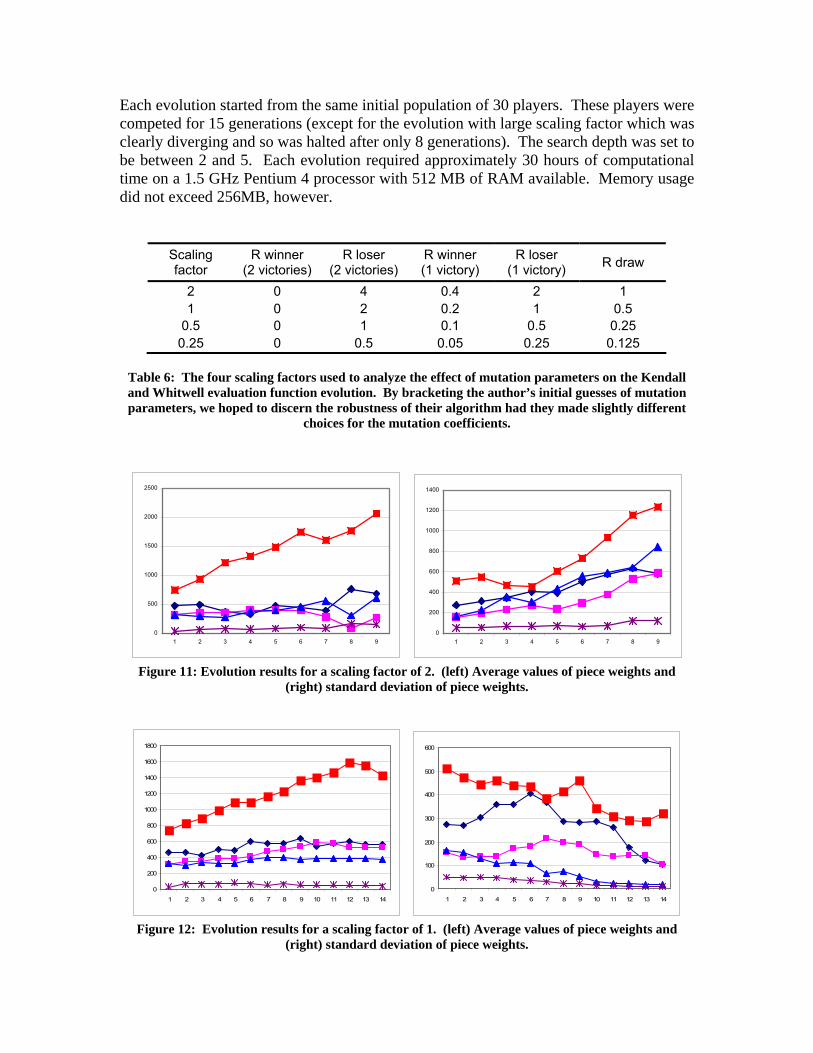
Each evolution started from the same initial population of 30 players. These players were competed for 15 generations (except for the evolution with large scaling factor which was clearly diverging and so was halted after only 8 generations). The search depth was set to be between 2 and 5. Each evolution required approximately 30 hours of computational time on a 1.5 GHz Pentium 4 processor with 512 MB of RAM available. Memory usage did not exceed 256MB, however.

Scaling factor

R winner (2 victories)

R loser (2 victories)

R winner (1 victory)

R loser (1 victory) R draw

2 0 4 0.4 2 1 1 0 2 0.2 1 0.5

0.5 0 1 0.1 0.5 0.25 0.25 0 0.5 0.05 0.25 0.125

Table 6: The four scaling factors used to analyze the effect of mutation parameters on the Kendall and Whitwell evaluation function evolution. By bracketing the author’s initial guesses of mutation parameters, we hoped to discern the robustness of their algorithm had they made slightly different

choices for the mutation coefficients.

0

500

1000

1500

2000

2500

1 2 3 4 5 6 7 8 9

0

200

400

600

800

1000

1 2 3 4 5 6 7 8 9

1200

1400

Figure 11: Evolution results for a scaling factor of 2. (left) Average values of piece weights and

(right) standard deviation of piece weights.

0

200

400

600

800

1000

1200

1400

1600

1800

1 2 3 4 5 6 7 8 9 10 11 12 13 14

0

100

200

300

400

500

600

1 2 3 4 5 6 7 8 9 10 11 12 13 14

Figure 12: Evolution results for a scaling factor of 1. (left) Average values of piece weights and

(right) standard deviation of piece weights.

0

200

400

600

800

1000

1200

1 2 3 4 5 6 7 8 9 10 11 12 13 14 15

0

100

200

300

400

500

600

1 2 3 4 5 6 7 8 9 10 11 12 13 14 15 16

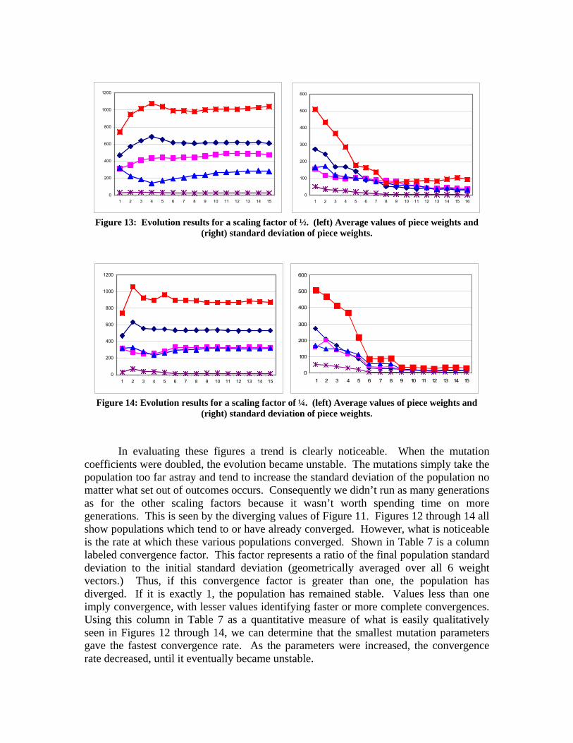
Figure 13: Evolution results for a scaling factor of ½. (left) Average values of piece weights and

(right) standard deviation of piece weights.

0

100

200

300

400

500

600

1 2 3 4 5 6 7 8 9 10 11 12 13 14 150

200

400

600

800

1000

1200

1 2 3 4 5 6 7 8 9 10 11 12 13 14 15

Figure 14: Evolution results for a scaling factor of ¼. (left) Average values of piece weights and

(right) standard deviation of piece weights. In evaluating these figures a trend is clearly noticeable. When the mutation coefficients were doubled, the evolution became unstable. The mutations simply take the population too far astray and tend to increase the standard deviation of the population no matter what set out of outcomes occurs. Consequently we didn’t run as many generations as for the other scaling factors because it wasn’t worth spending time on more generations. This is seen by the diverging values of Figure 11. Figures 12 through 14 all show populations which tend to or have already converged. However, what is noticeable is the rate at which these various populations converged. Shown in Table 7 is a column labeled convergence factor. This factor represents a ratio of the final population standard deviation to the initial standard deviation (geometrically averaged over all 6 weight vectors.) Thus, if this convergence factor is greater than one, the population has diverged. If it is exactly 1, the population has remained stable. Values less than one imply convergence, with lesser values identifying faster or more complete convergences. Using this column in Table 7 as a quantitative measure of what is easily qualitatively seen in Figures 12 through 14, we can determine that the smallest mutation parameters gave the fastest convergence rate. As the parameters were increased, the convergence rate decreased, until it eventually became unstable.

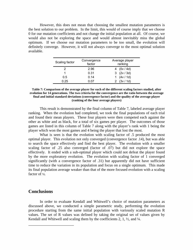
However, this does not mean that choosing the smallest mutation parameters is the best solution to our problem. In the limit, this would of course imply that we choose 0 for our mutation coefficients and not change the initial population at all. Of course, we would also not be exploring the space and would almost inevitably miss the global optimum. If we choose our mutation parameters to be too small, the evolution will definitely converge. However, it will not always converge to the most optimal solution available.

Scaling factor Convergence factor

Average player ranking

2 2.96 4 (0v / 4d) 1 0.31 3 (2v / 3d)

0.5 0.14 1 (4v / 1d) 0.25 0.07 2 (3v / 1d)

Table 7: Comparison of the average player for each of the different scaling factors studied, after

evolution for 14 generations. The two criteria for the convergence are the ratio between the average final and initial standard deviations (convergence factor) and the quality of the average player

(ranking of the four average players) This result is demonstrated by the final column of Table 7, labeled average player ranking. When the evolution had completed, we took the final populations of each trial and found their mean players. These four players were then competed each against the other as white and as black, for a total of six games per player. The outcomes of those games are listed in this column of Table 7 along with the player’s rank with 1 being the player which won the most games and 4 being the player that lost the most. What is seen is that the evolution with scaling factor of .5 produced the most optimal player. This evolution not only converged (convergence factor .14), but was able to search the space effectively and find the best player. The evolution with a smaller scaling factor of .25 also converged (factor of .07) but did not explore the space effectively. It ended with a sub-optimal player which could not defeat the player found by the more exploratory evolution. The evolution with scaling factor of 1 converged significantly (with a convergence factor of .31) but apparently did not have sufficient time to reduce the variation in its population and focus on a single optimum. This made its final population average weaker than that of the more focused evolution with a scaling factor of ½.

Conclusions

In order to evaluate Kendall and Whitwell’s choice of mutation parameters as discussed above, we conducted a simple parametric study, performing the evolution procedure starting from the same initial population with variously scaled mutation R values. The set of R values was defined by taking the original set of values given by Kendall and Whitwell and scaling them by the coefficients 2, 1, ½, and ¼.

We assert that the influence of the scaling factor was relatively easy to understand: if the factor was too high, the procedure did not converge, but if it was too low it converged toward a value close to the best seed in the initial population, even if that was not the global optimum. Such a situation makes the usage of evolutionary algorithms particularly dangerous in precisely the domains for which they were originally designed, those domains in which expert knowledge of the true solution is difficult or expensive to obtain. If a user is not careful to tweak the mutation parameters many times and discover the dependence of the solution on them, his algorithm may seem to converge, but may be converging to a horribly sub-optimal value. The scaling factor must be high enough to explore the space and be sure to eventually include the global optimum into the population, but low enough to quickly converge toward this optimum solution.

Obviously finding the best scaling factor is itself a difficult problem which could be represented by a maximization statement in its own one-dimensional space. The “Holy Grail” might in fact be to evolve the evolution procedure in order to find the set of R coefficients that lead to the fastest and most accurate convergence. We can do this by applying the same procedure that is used to evolve the seeds of the evaluation function. Starting from a random population of R values we can use each of them to evolve an evaluation function from the same initial population. Even if several sets of R coefficients from the R population should lead to approximately the same player in terms of the evaluation function, the number of generations to converge would be different. There would also be sets of R with too small of a scaling factor whose populations would converge toward a non-optimum player. To assess which set of R is better, we could have play-offs between the averages of the populations obtained after a certain number of generations. Then we would keep the “good” set of R values, replace the less fit members by mutated clones of the good ones, and do the procedure again until we converge toward a final set of R coefficients. Unfortunately, however, such a technique requires immense amounts of possibly expensive computation. Perhaps this instability and lack of robustness to slight algorithmic changes are two of the reasons evolutionary algorithms have long remained an interesting, shot-in-the-dark alternative to conventional optimization methods, but have not been adequately generalized to the solution of arbitrary problems. With more study and sufficient computational resources, we hope future researchers can more deeply investigate and perhaps find some theoretical basis for the variation of evolutionary convergence with changing mutation parameters. As it stands, our study should serve as a caution to future implementers: An evolutionary algorithm must be finely honed and sufficiently investigated in domains of partial or complete knowledge before being applied to a domain with unpredictable results.

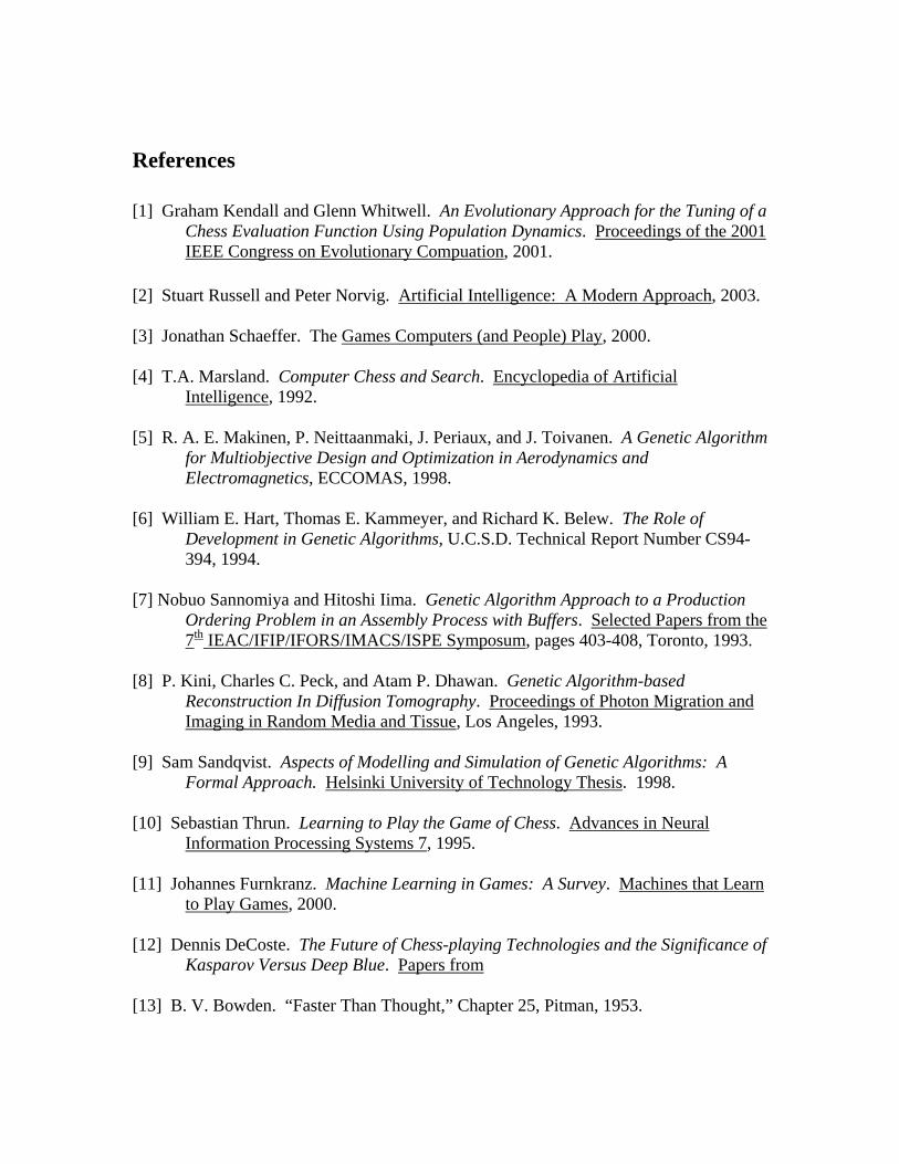
References [1] Graham Kendall and Glenn Whitwell. An Evolutionary Approach for the Tuning of a

Chess Evaluation Function Using Population Dynamics. Proceedings of the 2001 IEEE Congress on Evolutionary Compuation, 2001.

[2] Stuart Russell and Peter Norvig. Artificial Intelligence: A Modern Approach, 2003. [3] Jonathan Schaeffer. The Games Computers (and People) Play, 2000. [4] T.A. Marsland. Computer Chess and Search. Encyclopedia of Artificial

Intelligence, 1992. [5] R. A. E. Makinen, P. Neittaanmaki, J. Periaux, and J. Toivanen. A Genetic Algorithm

for Multiobjective Design and Optimization in Aerodynamics and Electromagnetics, ECCOMAS, 1998.

[6] William E. Hart, Thomas E. Kammeyer, and Richard K. Belew. The Role of

Development in Genetic Algorithms, U.C.S.D. Technical Report Number CS94-394, 1994.

[7] Nobuo Sannomiya and Hitoshi Iima. Genetic Algorithm Approach to a Production

Ordering Problem in an Assembly Process with Buffers. Selected Papers from the 7th IEAC/IFIP/IFORS/IMACS/ISPE Symposum, pages 403-408, Toronto, 1993.

[8] P. Kini, Charles C. Peck, and Atam P. Dhawan. Genetic Algorithm-based

Reconstruction In Diffusion Tomography. Proceedings of Photon Migration and Imaging in Random Media and Tissue, Los Angeles, 1993.

[9] Sam Sandqvist. Aspects of Modelling and Simulation of Genetic Algorithms: A

Formal Approach. Helsinki University of Technology Thesis. 1998. [10] Sebastian Thrun. Learning to Play the Game of Chess. Advances in Neural

Information Processing Systems 7, 1995. [11] Johannes Furnkranz. Machine Learning in Games: A Survey. Machines that Learn

to Play Games, 2000. [12] Dennis DeCoste. The Future of Chess-playing Technologies and the Significance of

Kasparov Versus Deep Blue. Papers from [13] B. V. Bowden. “Faster Than Thought,” Chapter 25, Pitman, 1953.