Embed Size (px)
Citation preview
ARMY RESEARCH LABORATORY
An Experiment, Analysis, and Model of Ballistic Shock
by J. Terrence Klopcic, Walton T. Robinson, Donald W. Petty, and Michael R. Sivack
ARL-MR-368 November 1997
wnm m
Approved for public release; distribution is unlimited.

The findings in this report are not to be construed as an official Department of the Army position unless so designated by other authorized documents.
Citation of manufacturer's or trade names does not constitute an official endorsement or approval of the use thereof.
Destroy this report when it is no longer needed. Do not return it to the originator.
Army Research Laboratory Aberdeen Proving Ground, MD 21005-5068
ARL-MR-368 November 1997
An Experiment, Analysis, and Model of Ballistic Shock
J. Terrence Klopcic, Walton T. Robinson, Donald W. Petty, Michael R. Sivack Survivability/Lethality Analysis Directorate, ARL
[BEG QÜALHY INSPECTED S
Approved for public release; distribution is unlimited.
Abstract
This study deals with the propagation of the leading, high-frequency edge of the shock wave emanating from an impact point on an armored vehicle, specifically, in an experiment on an Ml 13 armored personnel carrier subjected to explosive charges.
The amplitude of the transverse wave can be well fit by a semiempirical equation, which accounts for both longitudinal and transverse waves, exponential decrease with distance, mixing of waves at edges, and amplification at points near edges. Comparison of wave speeds with published data confirms the roles of longitudinal and transverse disturbances.
u

Acknowledgments
The authors wish to acknowledge the superb guidance and support given to us by Mr. Joseph Collins of the U.S. Army Research Laboratory (ARL). Joe pro- vided not only the software, but also the dedicated training on that software, which allowed us to conduct the analysis presented here.
The willingness and expertise of Dr. Barry Bodt of ARL to supply guidance on statistical matters, on this project as well as on many others over the years, are gratefully acknowledged.
in

This page intentionally left blank
IV
Contents
Acknowledgments m
I. Introduction 1
II. Experimental Procedure and Results 3
III. Analysis 8
A. Extraction of Metrics 8
1. Pulse Shape Analysis 8
2. Arrival Time Analysis • • 9
3. Amplitude Metrics. 12
4. Semi-empirical Equation Development 16
5. Goodness of Fit 20
IV. Summary and Discussion 23
Appendix A: Calibrated Data 25
Appendix B: Normalized Data - Each Shot 123

This page intentionally left blank
VI
List of Figures
1 Gauge Positions on M113, Top View 4
2 Gauge Positions on M113, Side Views 5
3 Calibrated Output of Gauge #6, Shot #709 .......... 7
4 Arrival Time of Precursor Pulse - Top Gauges 10
5 Arrival Time of Main Pulse - Top Gauges 10
6 Arrival Time of Main Pulse - Front and Top Gauges 11
7 Calibrated Output of Gauge #4, Shot #713 13
8 Calibrated Output of Gauge #4, Shot #708 14
9 Pulse Amplitudes by Distance from Shock Point 17
10 Fit to Pulse Amplitudes by Distance from Shock Point. .... 19
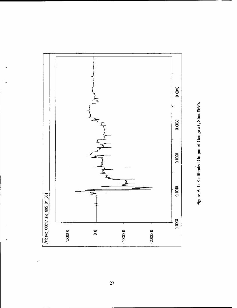
A-l Calibrated Output of Gauge #1, Shot #695 27
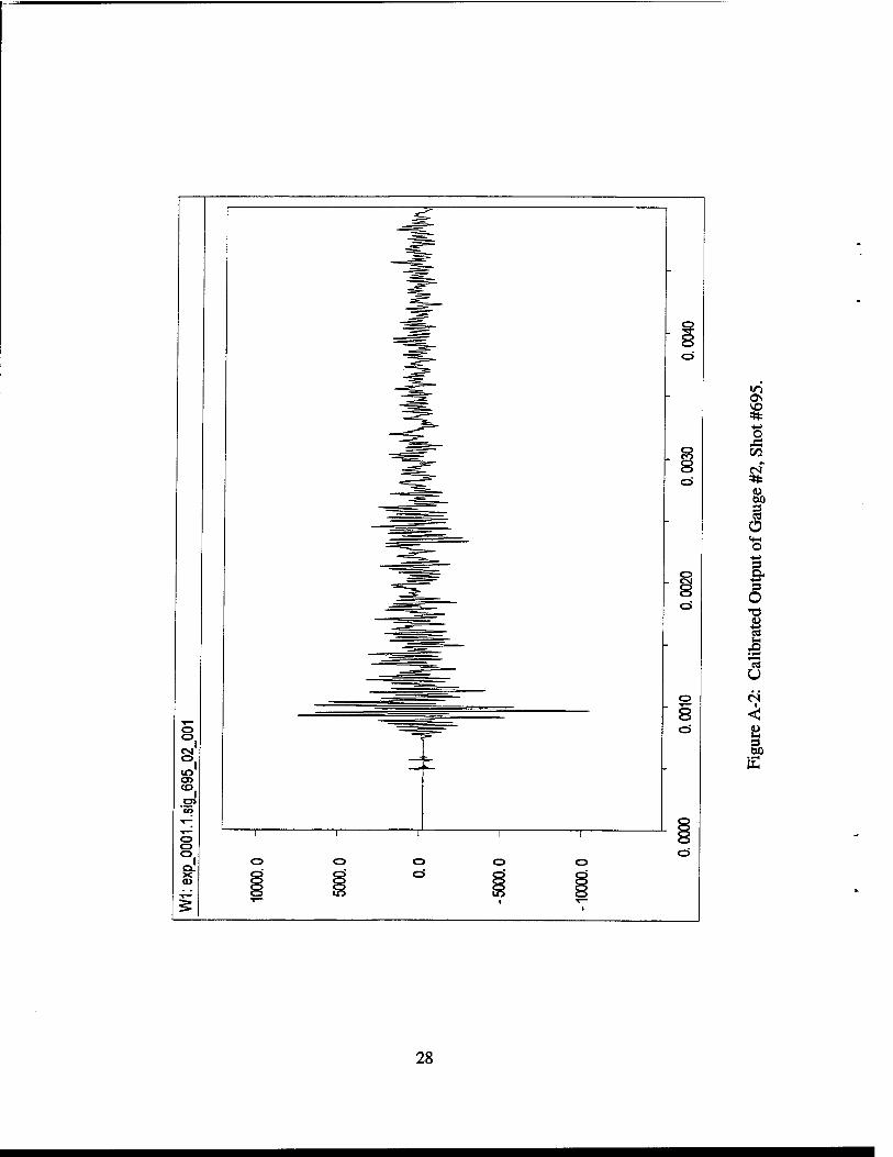
A-2 Calibrated Output of Gauge #2, Shot #695 28
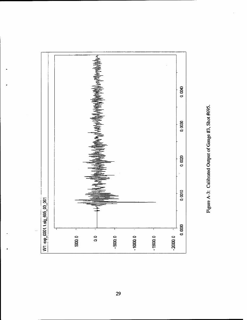
A-3 Calibrated Output of Gauge #3, Shot #695 29
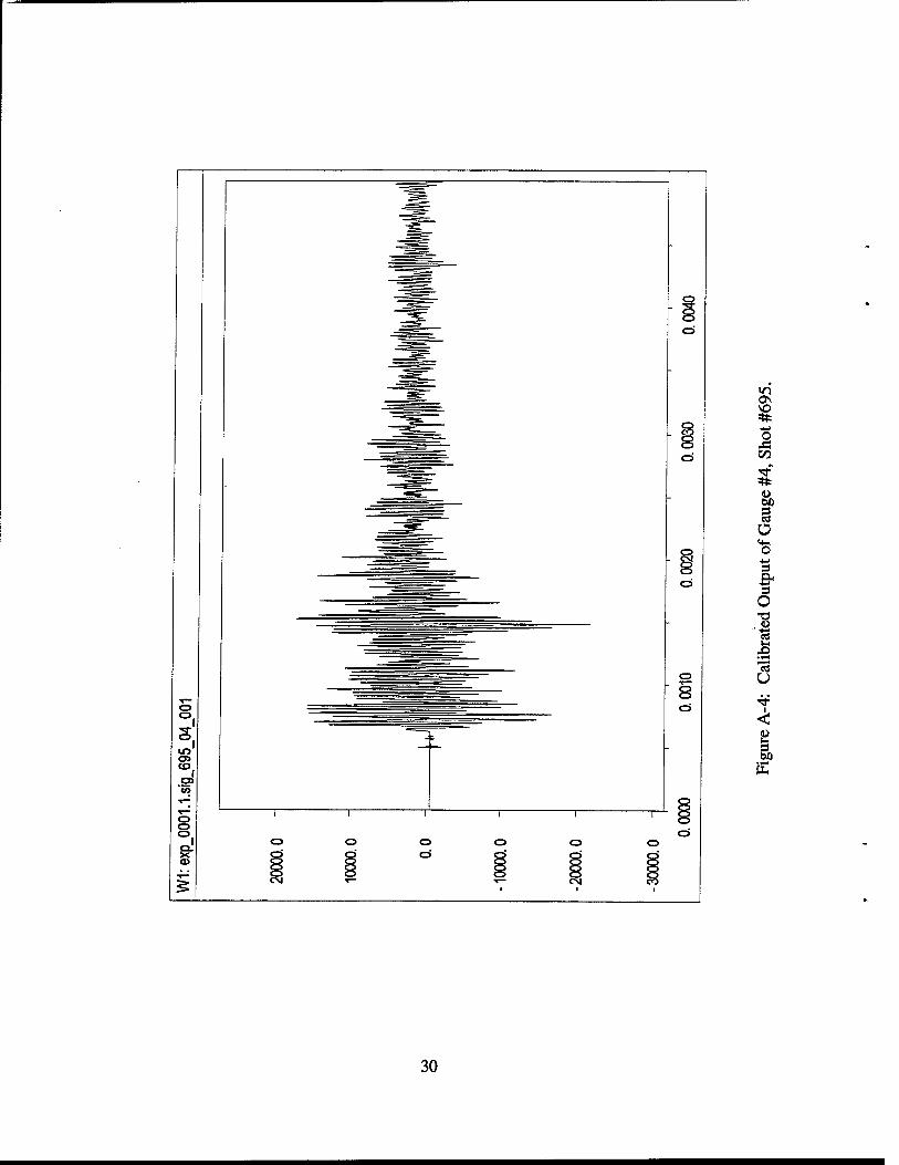
A-4 Calibrated Output of Gauge #4, Shot #695 30
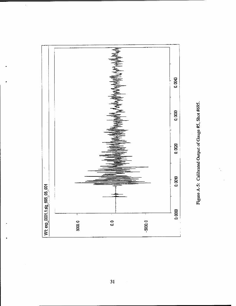
A-5 Calibrated Output of Gauge #5, Shot #695 31
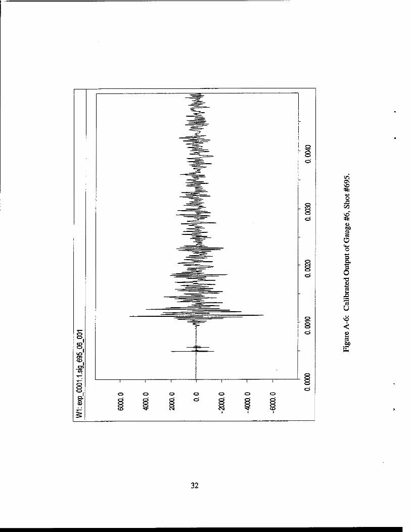
A-6 Calibrated Output of Gauge #6, Shot #695 32
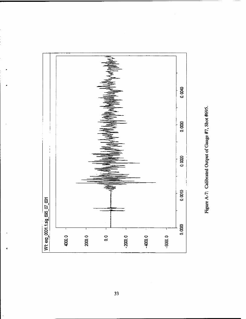
A-7 Calibrated Output of Gauge #7, Shot #695 33
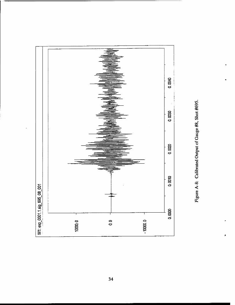
A-8 Calibrated Output of Gauge #8, Shot #695 34
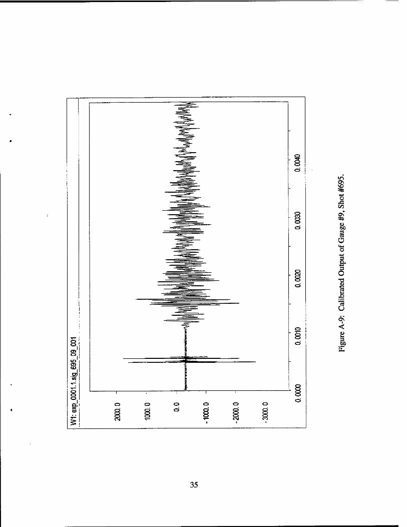
A-9 Calibrated Output of Gauge #9, Shot #695 35
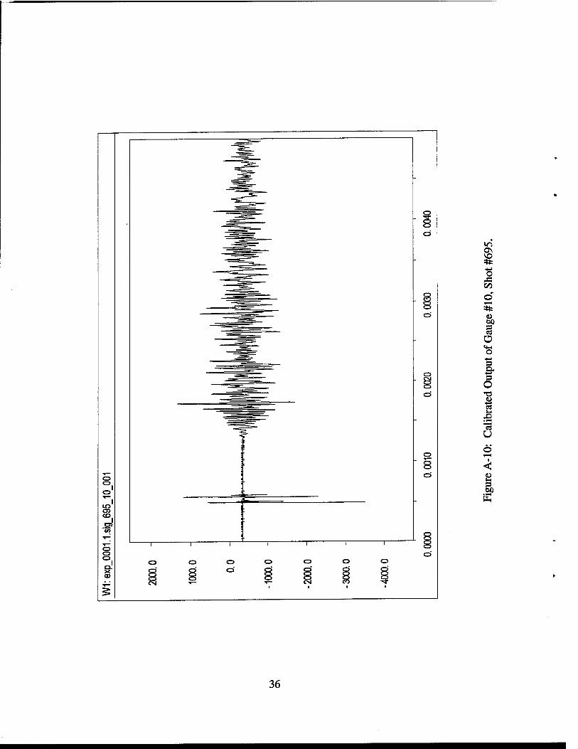
A-10 Calibrated Output of Gauge #10, Shot #695 36
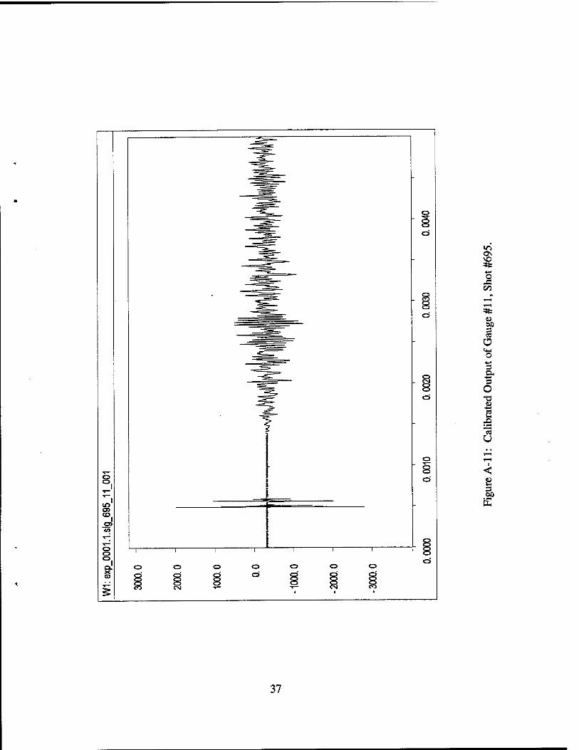
A-ll Calibrated Output of Gauge #11, Shot #695 37
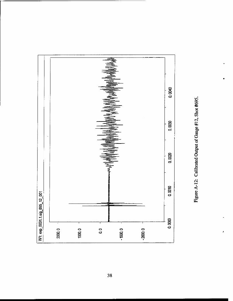
A-12 Calibrated Output of Gauge #12, Shot #695 38
vii
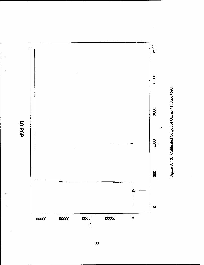
A-13 Calibrated Output of Gauge #1, Shot #698 39
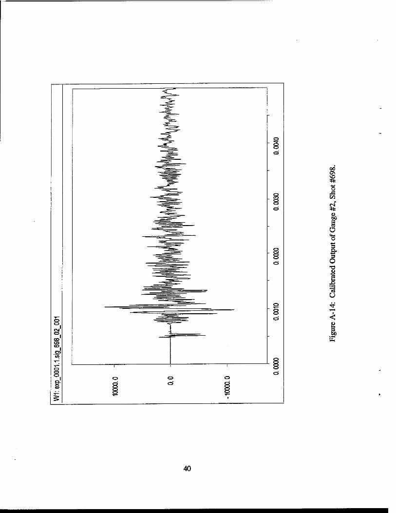
A-14 Calibrated Output of Gauge #2, Shot #698 40
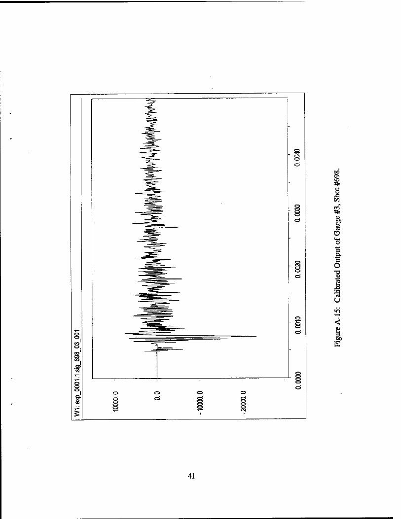
A-15 Calibrated Output of Gauge #3, Shot #698 41
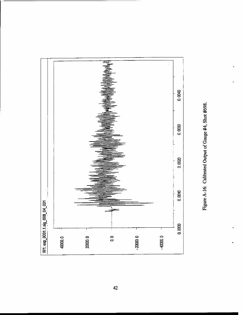
A-16 Calibrated Output of Gauge #4, Shot #698 42
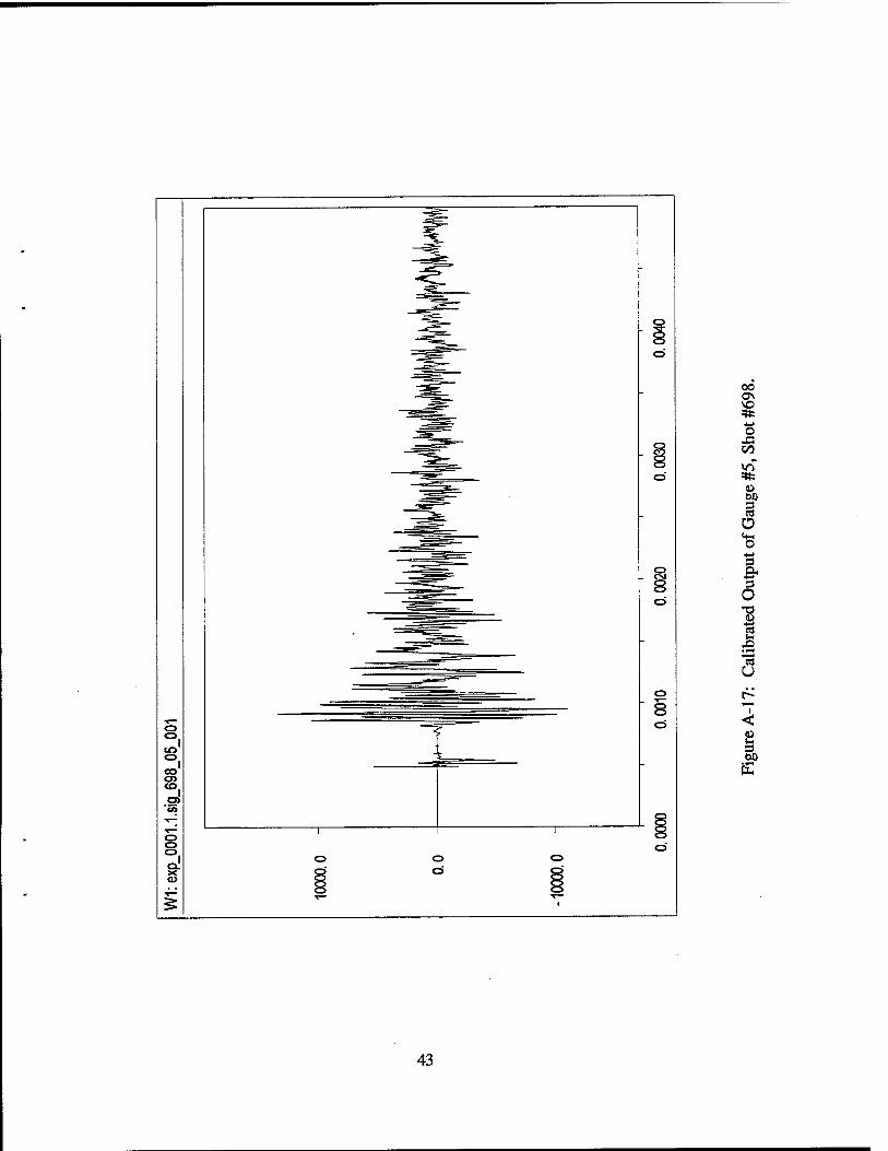
A-17 Calibrated Output of Gauge #5, Shot #698 43
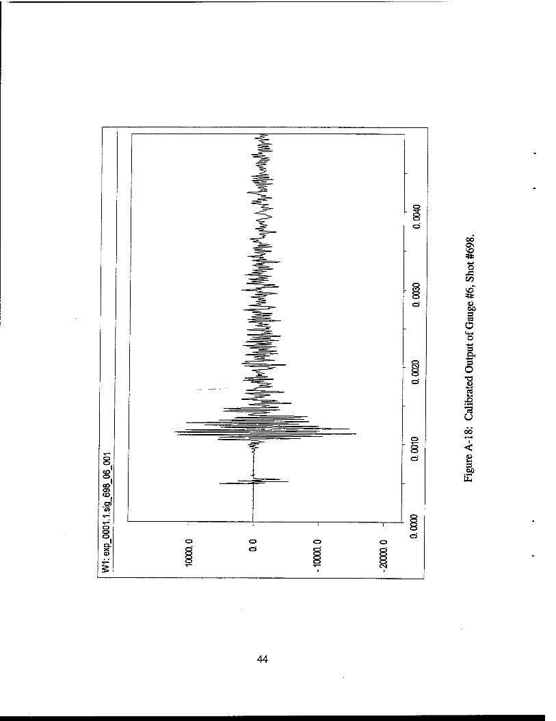
A-18 Calibrated Output of Gauge #6, Shot #698 44
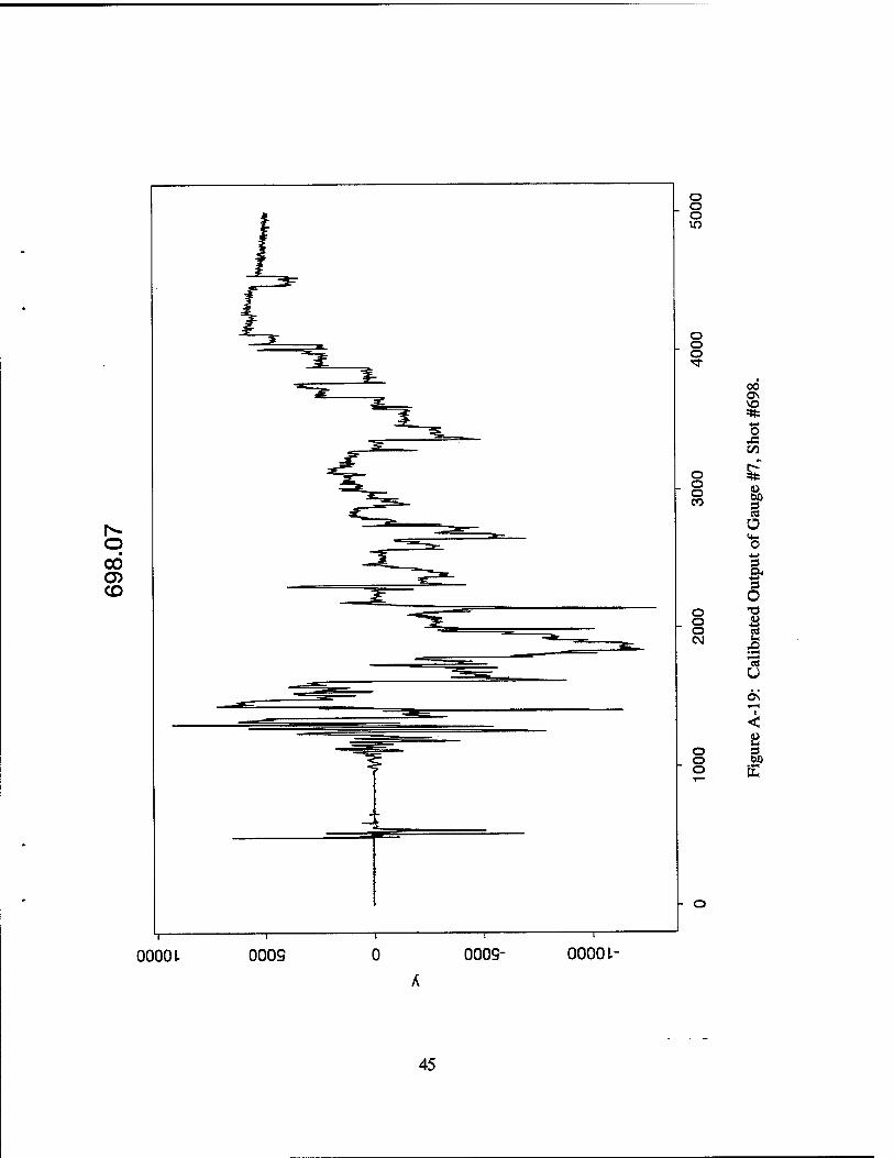
A-19 Calibrated Output of Gauge #7, Shot #698 45
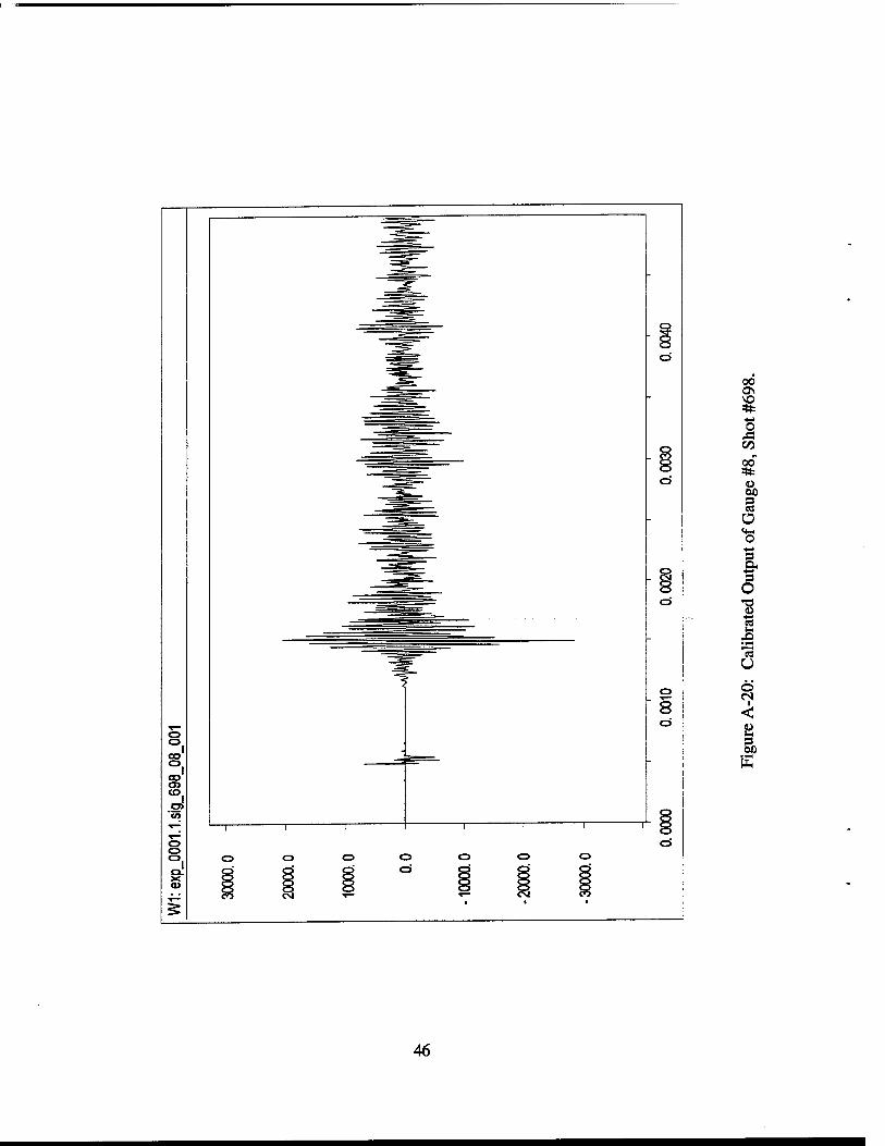
A-20 Calibrated Output of Gauge #8, Shot #698 46
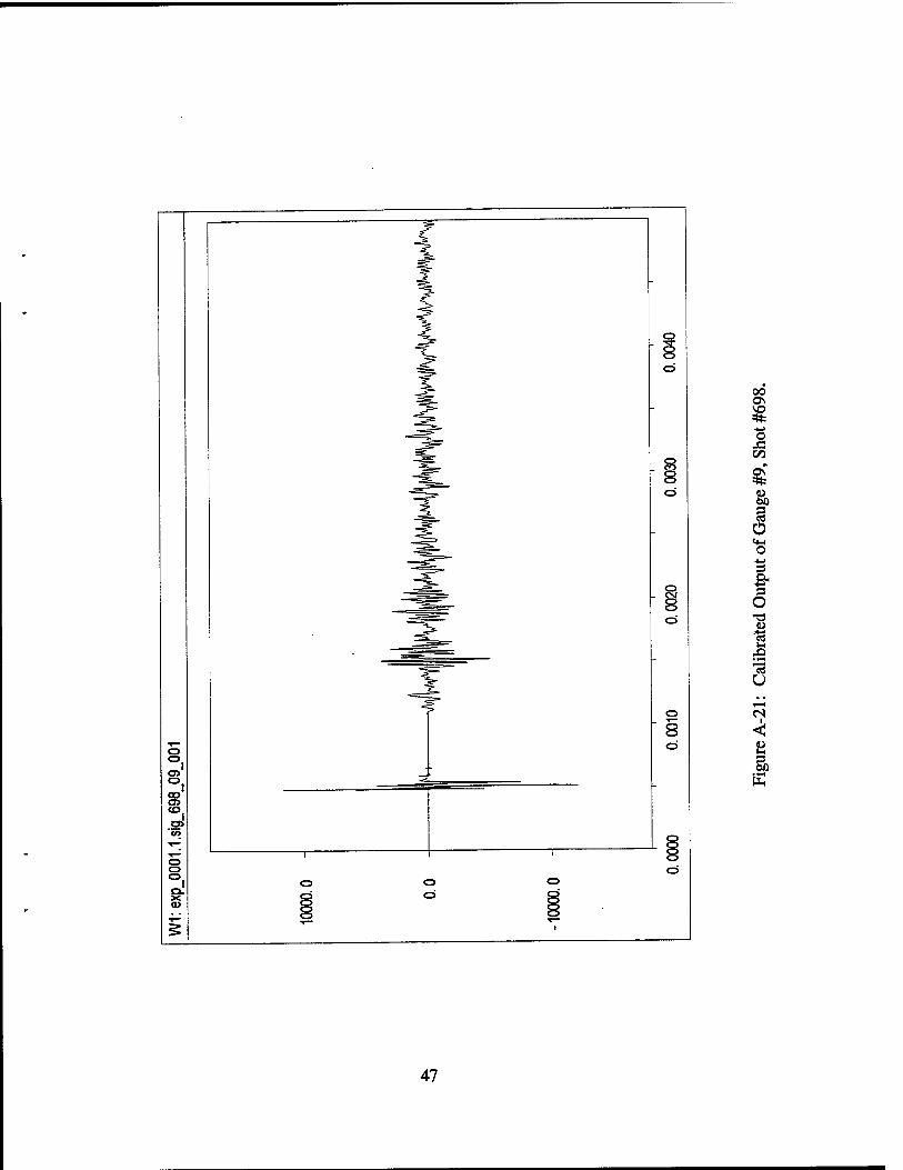
A-21 Calibrated Output of Gauge #9, Shot #698 47
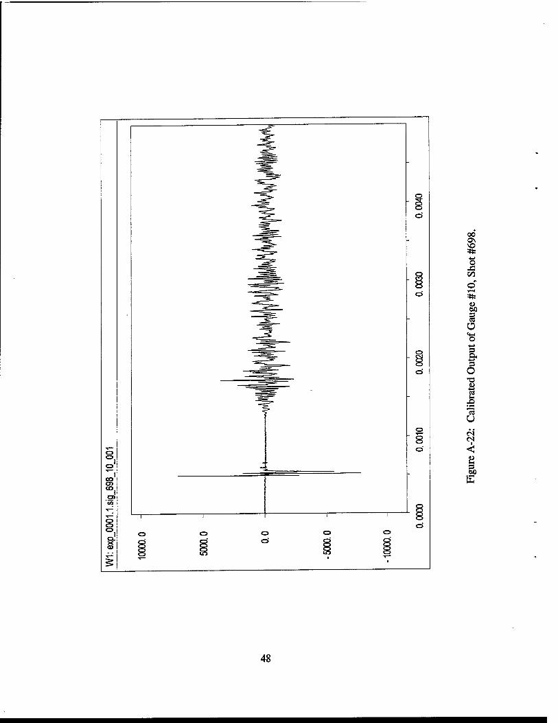
A-22 Calibrated Output of Gauge #10, Shot #698 48
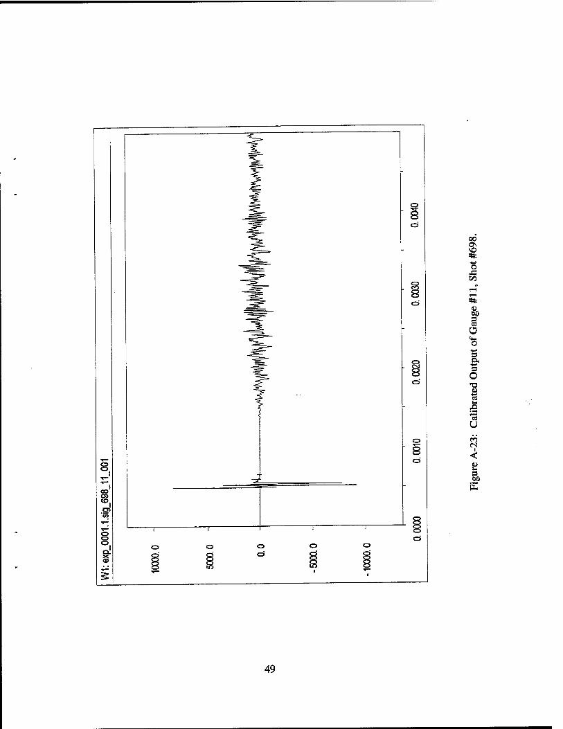
A-23 Calibrated Output of Gauge #11, Shot #698 49
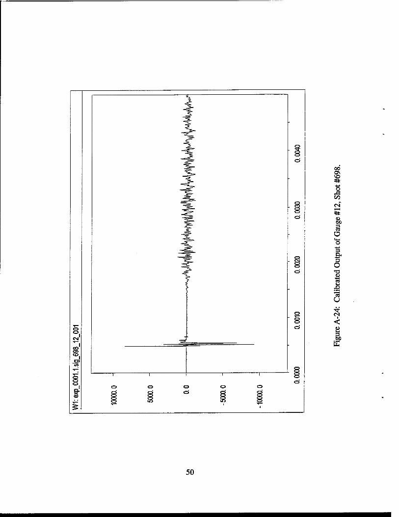
A-24 Calibrated Output of Gauge #12, Shot #698 50
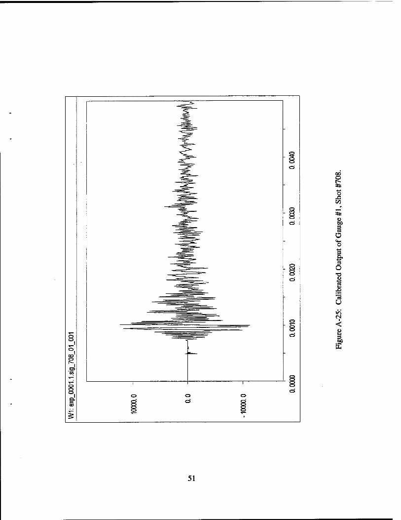
A-25 Calibrated Output of Gauge #1, Shot #708 51
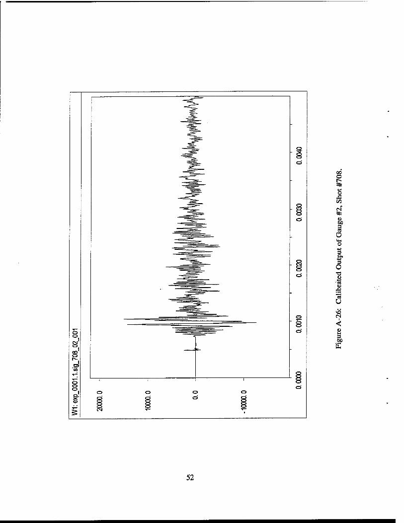
A-26 Calibrated Output of Gauge #2, Shot #708 52
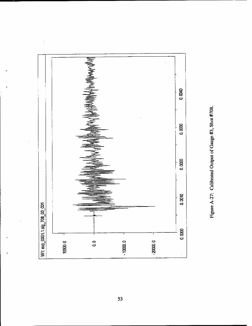
A-27 Calibrated Output of Gauge #3, Shot #708 53
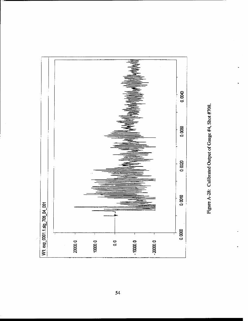
A-28 Calibrated Output of Gauge #4, Shot #708 54
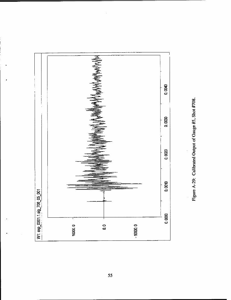
A-29 Calibrated Output of Gauge #5, Shot #708 55
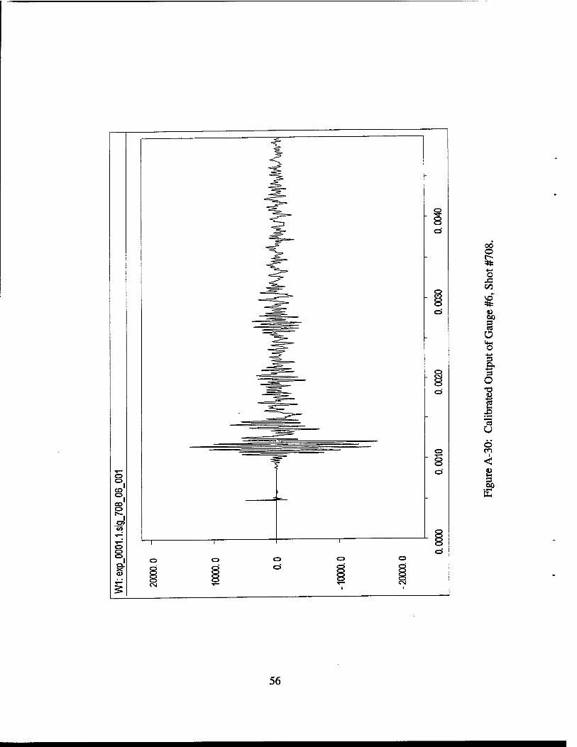
A-30 Calibrated Output of Gauge #6, Shot #708 56
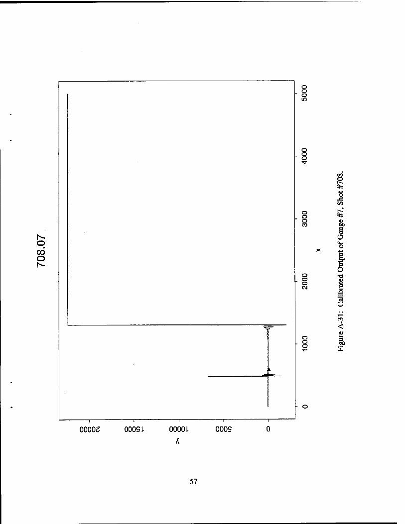
A-31 Calibrated Output of Gauge #7, Shot #708 57
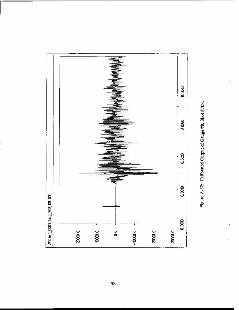
A-32 Calibrated Output of Gauge #8, Shot #708 58
A-33 Calibrated Output of Gauge #9, Shot #708 59
A-34 Calibrated Output of Gauge #10, Shot #708 60
A-35 Calibrated Output of Gauge #11, Shot #708 61
vm
A-36 Calibrated Output of Gauge #12, Shot #708 62
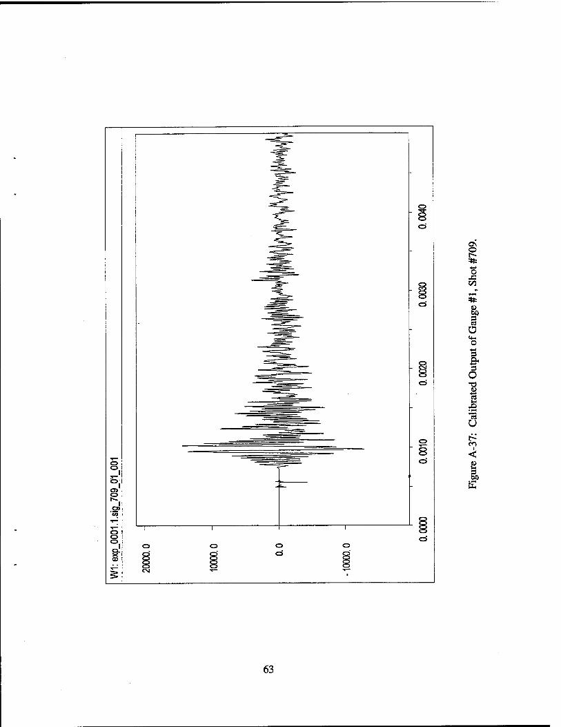
A-37 Calibrated Output of Gauge #1, Shot #709 63
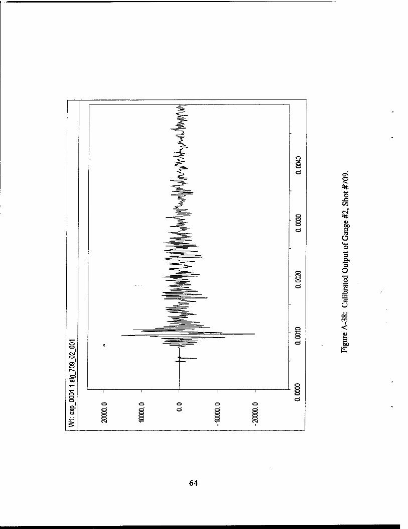
A-38 Calibrated Output of Gauge #2, Shot #709 64
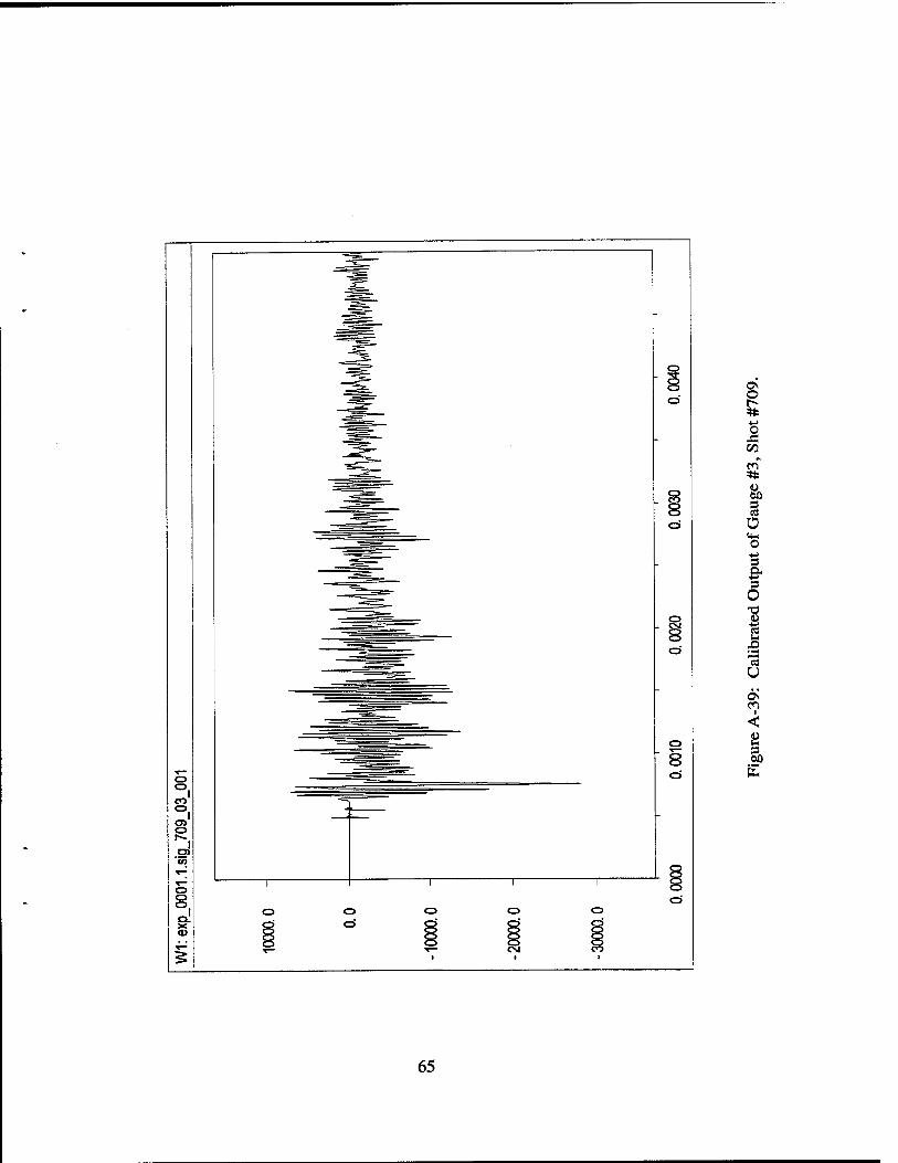
A-39 Calibrated Output of Gauge #3, Shot #709 65
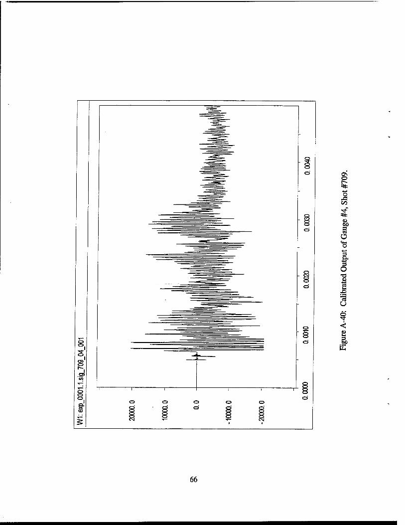
A-40 Calibrated Output of Gauge #4, Shot #709 66
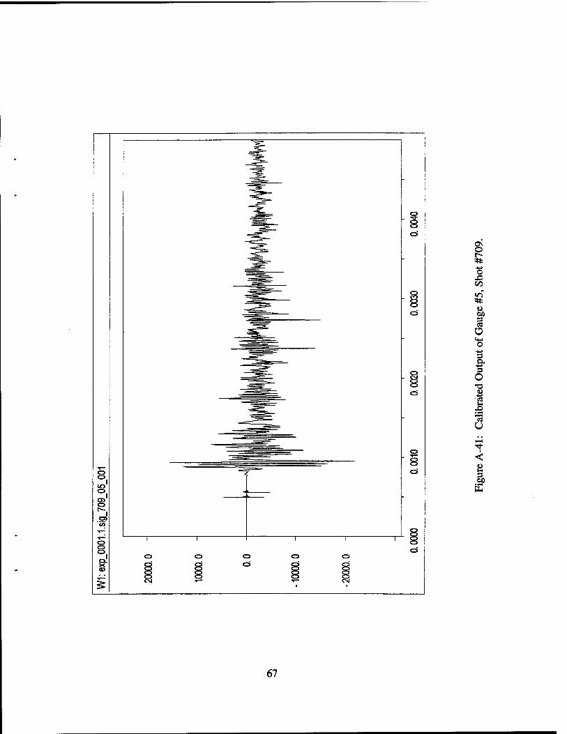
A-41 Calibrated Output of Gauge #5, Shot #709 67
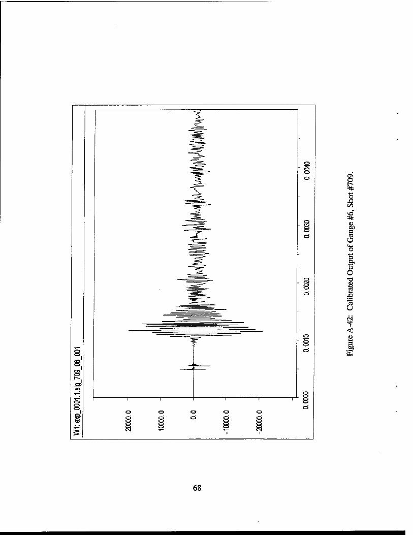
A-42 Calibrated Output of Gauge #6, Shot #709 68
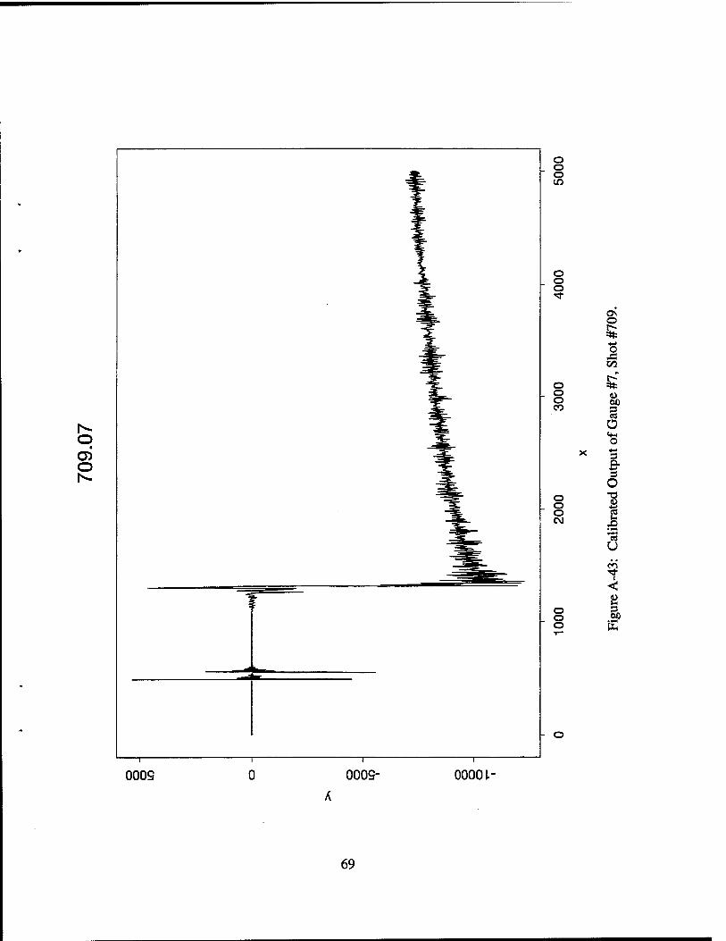
A-43 Calibrated Output of Gauge #7, Shot #709 69
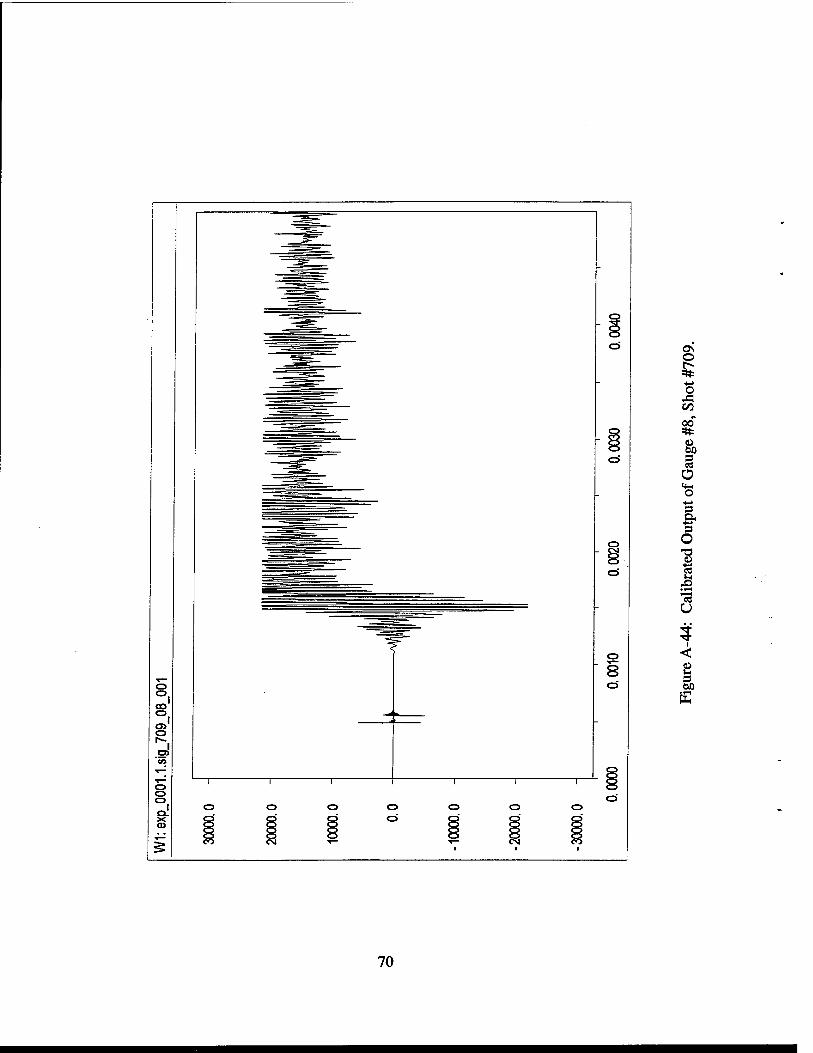
A-44 Calibrated Output of Gauge #8, Shot #709 70
A-45 Calibrated Output of Gauge #9, Shot #709 71
A-46 Calibrated Output of Gauge #10, Shot #709 72
A-47 Calibrated Output of Gauge #11, Shot #709 73
A-48 Calibrated Output of Gauge #12, Shot #709 74
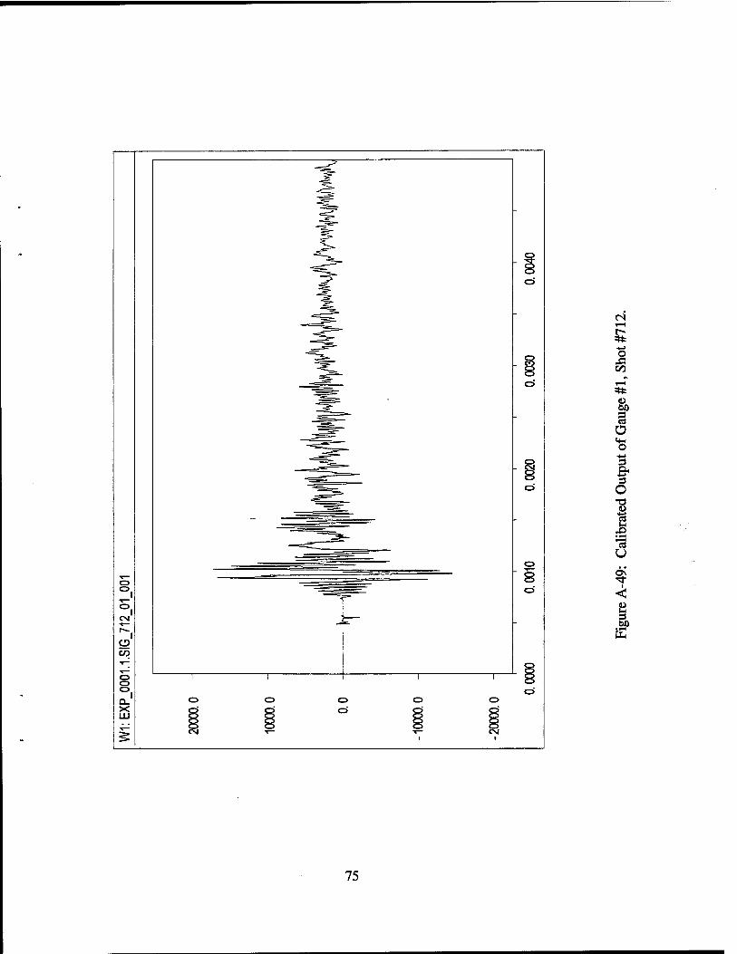
A-49 Calibrated Output of Gauge #1, Shot #712 75
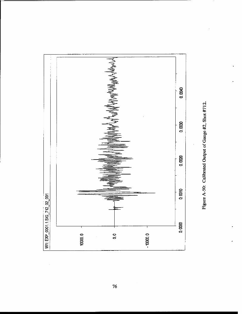
A-50 Calibrated Output of Gauge #2, Shot #712 76
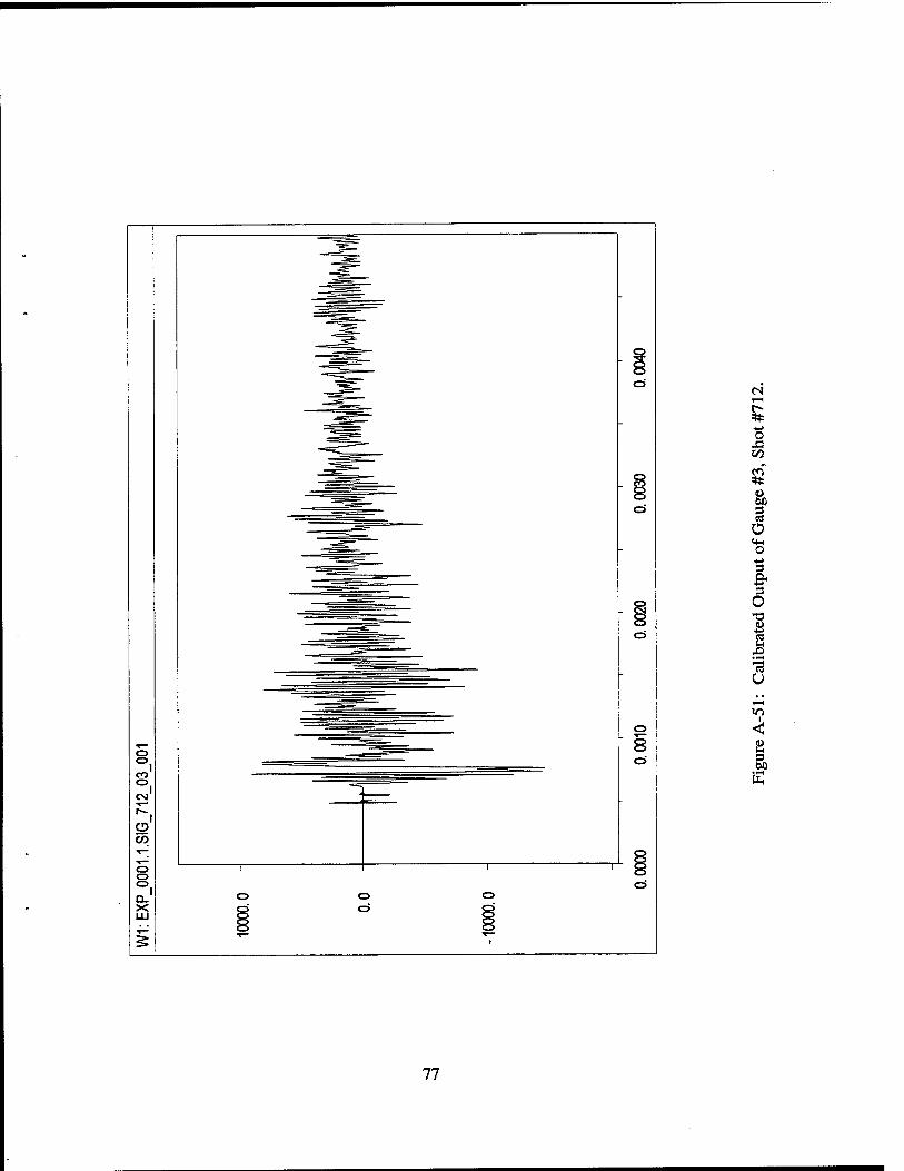
A-51 Calibrated Output of Gauge #3, Shot #712 77
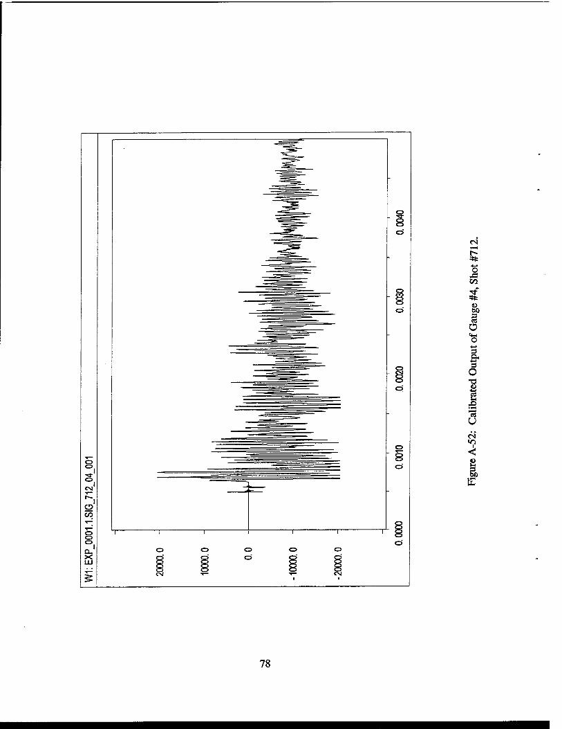
A-52 Calibrated Output of Gauge #4, Shot #712 78
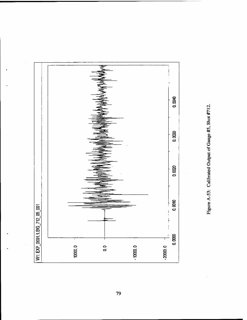
A-53 Calibrated Output of Gauge #5, Shot #712 79
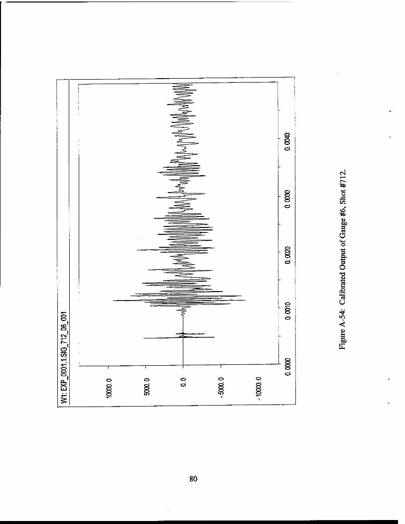
A-54 Calibrated Output of Gauge #6, Shot #712 80
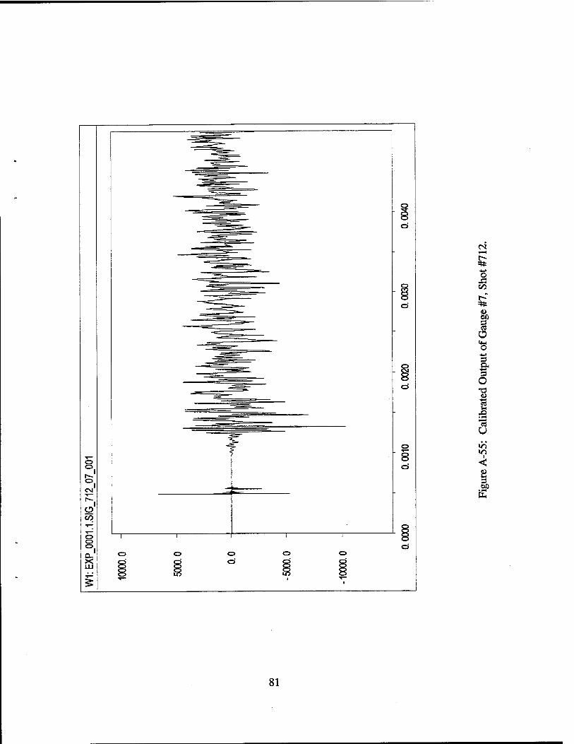
A-55 Calibrated Output of Gauge #7, Shot #712 81
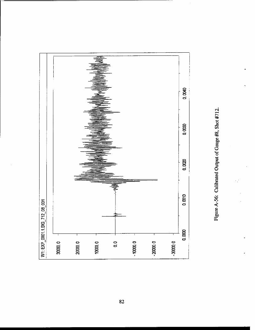
A-56 Calibrated Output of Gauge #8, Shot #712 82
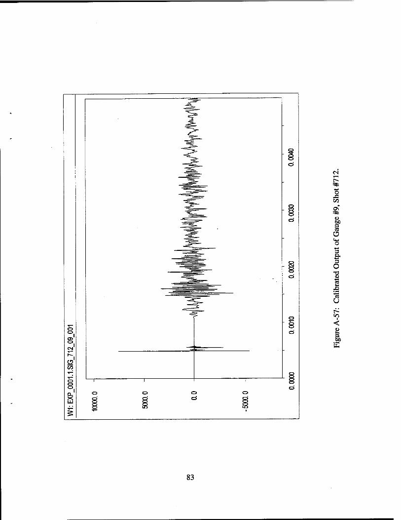
A-57 Calibrated Output of Gauge #9, Shot #712 83
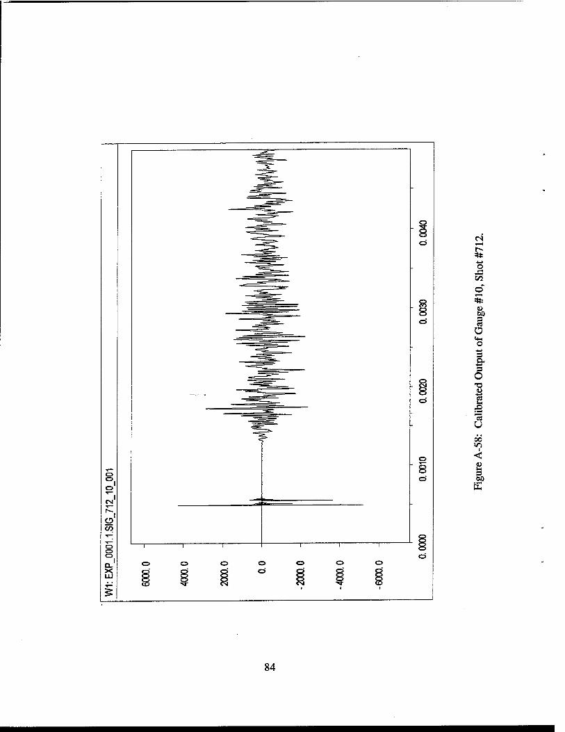
A-58 Calibrated Output of Gauge #10, Shot #712 84
IX
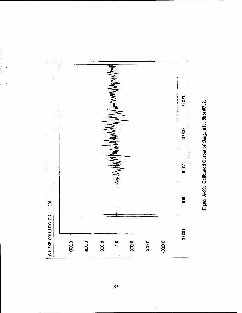
A-59 Calibrated Output of Gauge #11, Shot #712 85
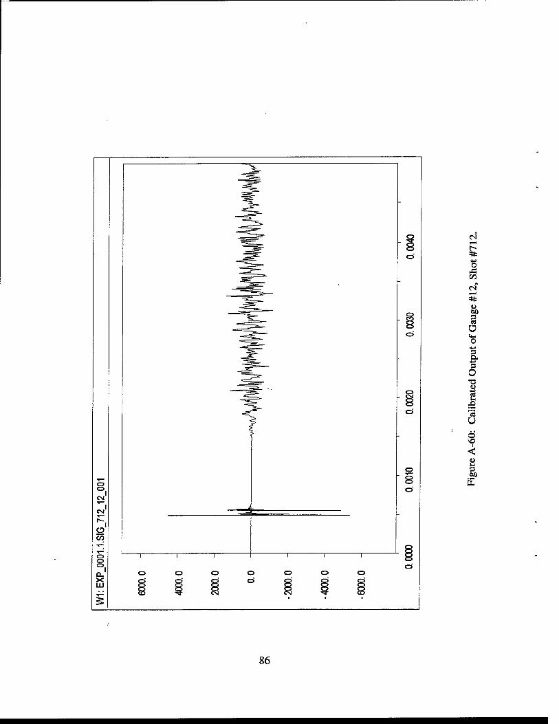
A-60 Calibrated Output of Gauge #12, Shot #712 86
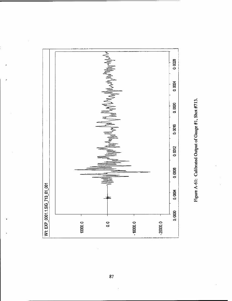
A-61 Calibrated Output of Gauge #1, Shot #713 87
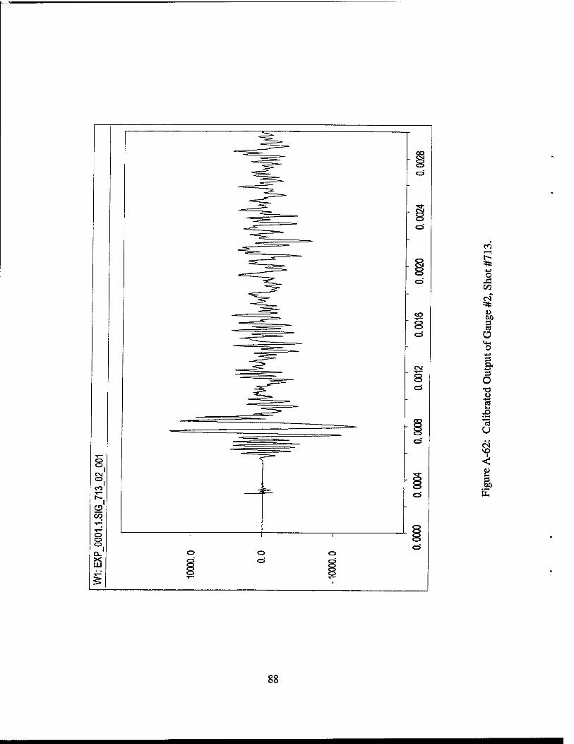
A-62 Calibrated Output of Gauge #2, Shot #713 88
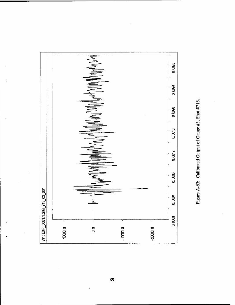
A-63 Calibrated Output of Gauge #3, Shot #713 89
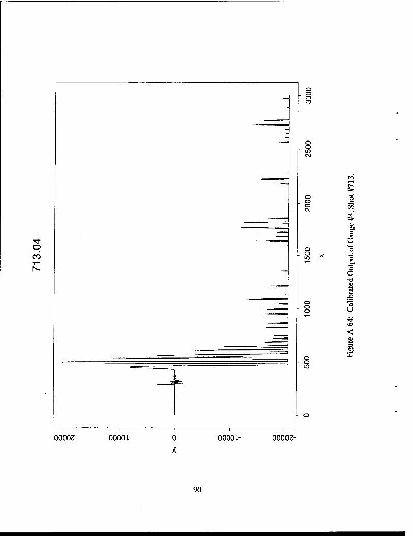
A-64 Calibrated Output of Gauge #4, Shot #713 90
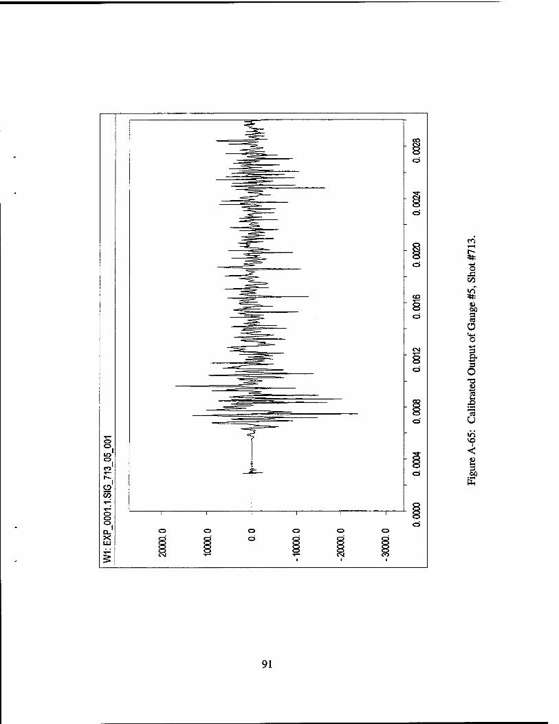
A-65 Calibrated Output of Gauge #5, Shot #713 91
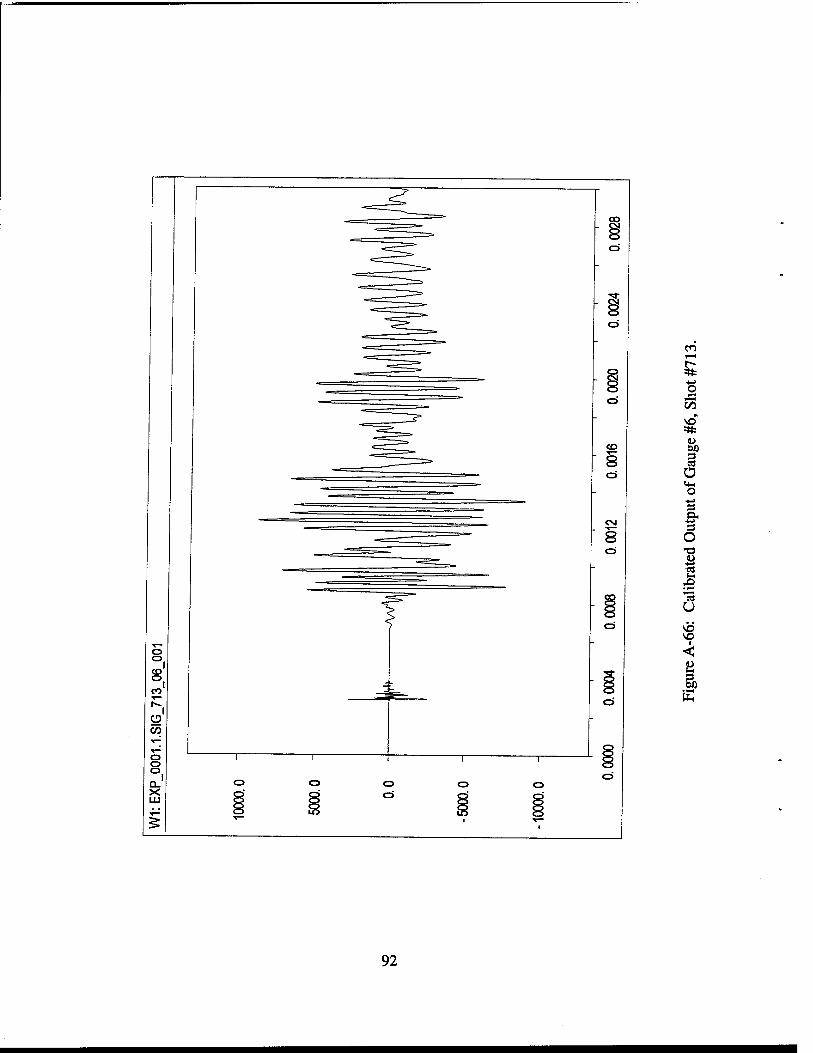
A-66 Calibrated Output of Gauge #6, Shot #713 92
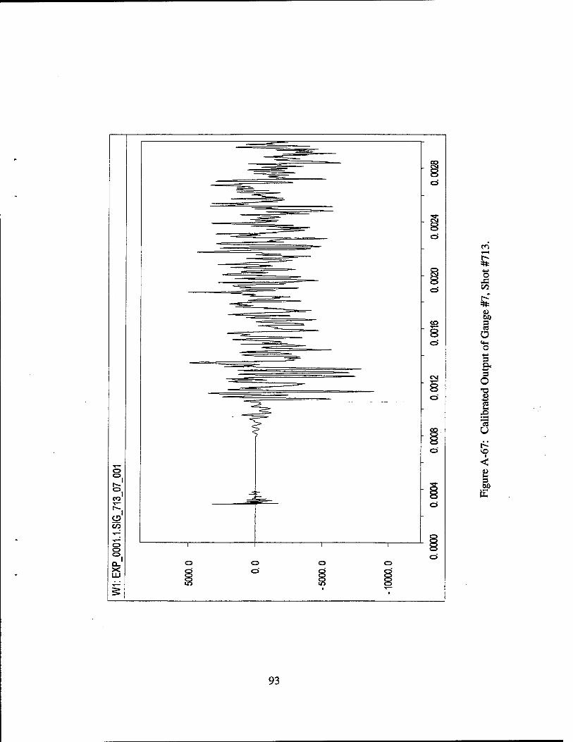
A-67 Calibrated Output of Gauge #7, Shot #713 93
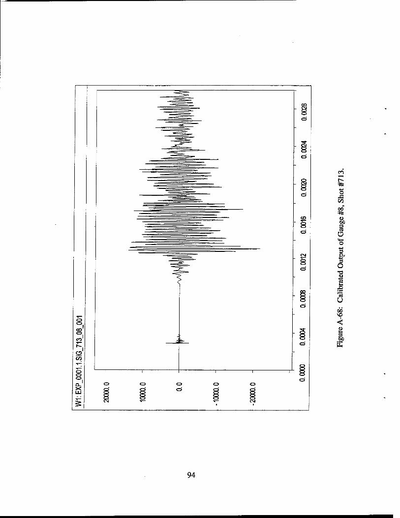
A-68 Calibrated Output of Gauge #8, Shot #713 94
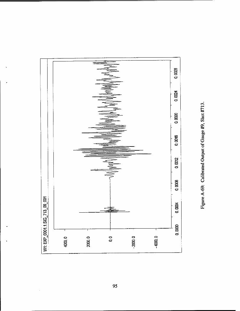
A-69 Calibrated Output of Gauge #9, Shot #713 95
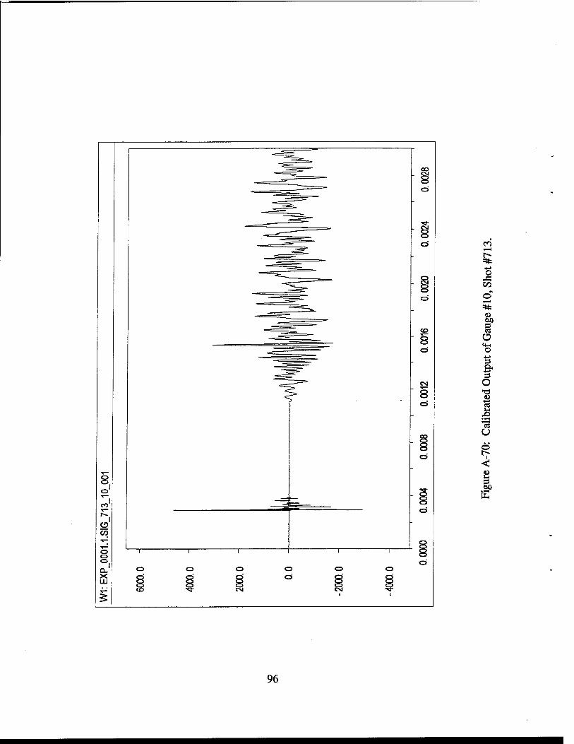
A-70 Calibrated Output of Gauge #10, Shot #713 96
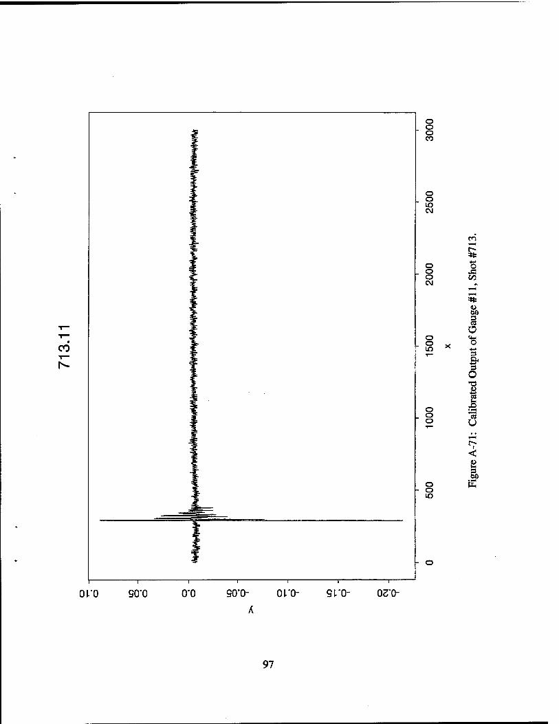
A-71 Calibrated Output of Gauge #11, Shot #713 97
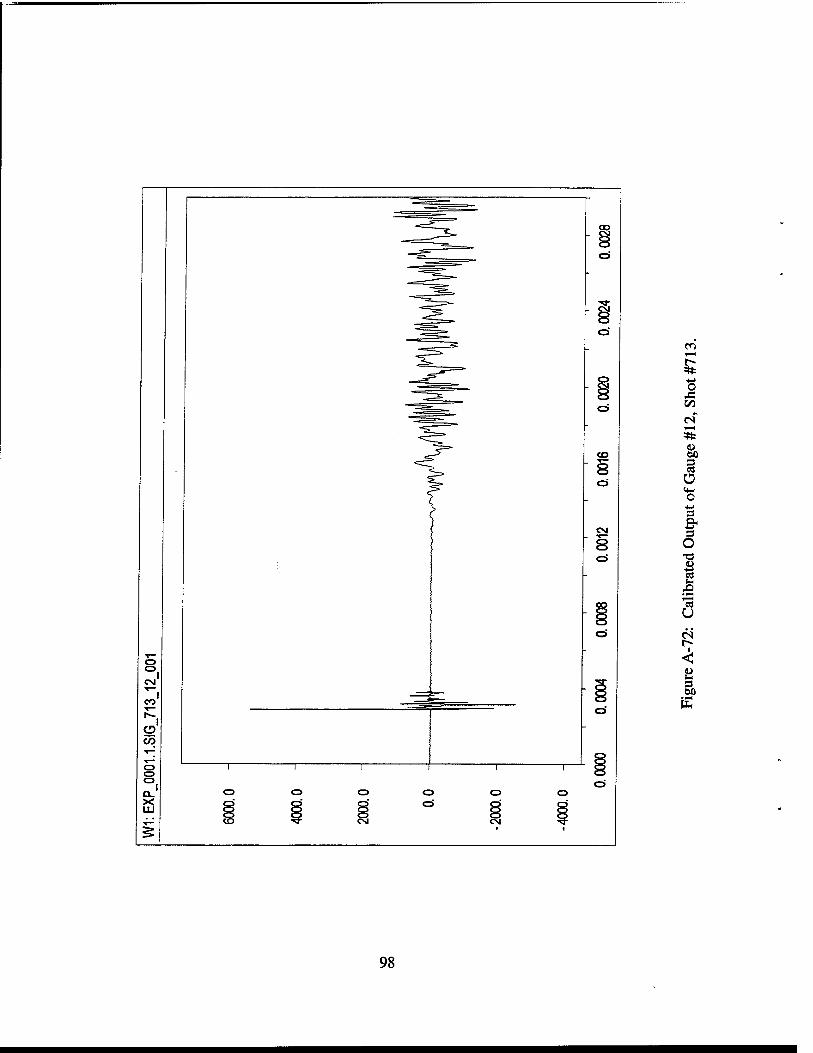
A-72 Calibrated Output of Gauge #12, Shot #713 98
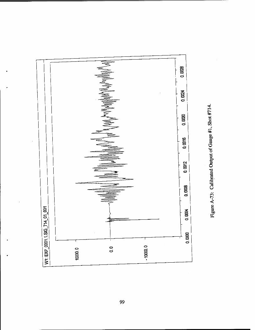
A-73 Calibrated Output of Gauge #1, Shot #714 99
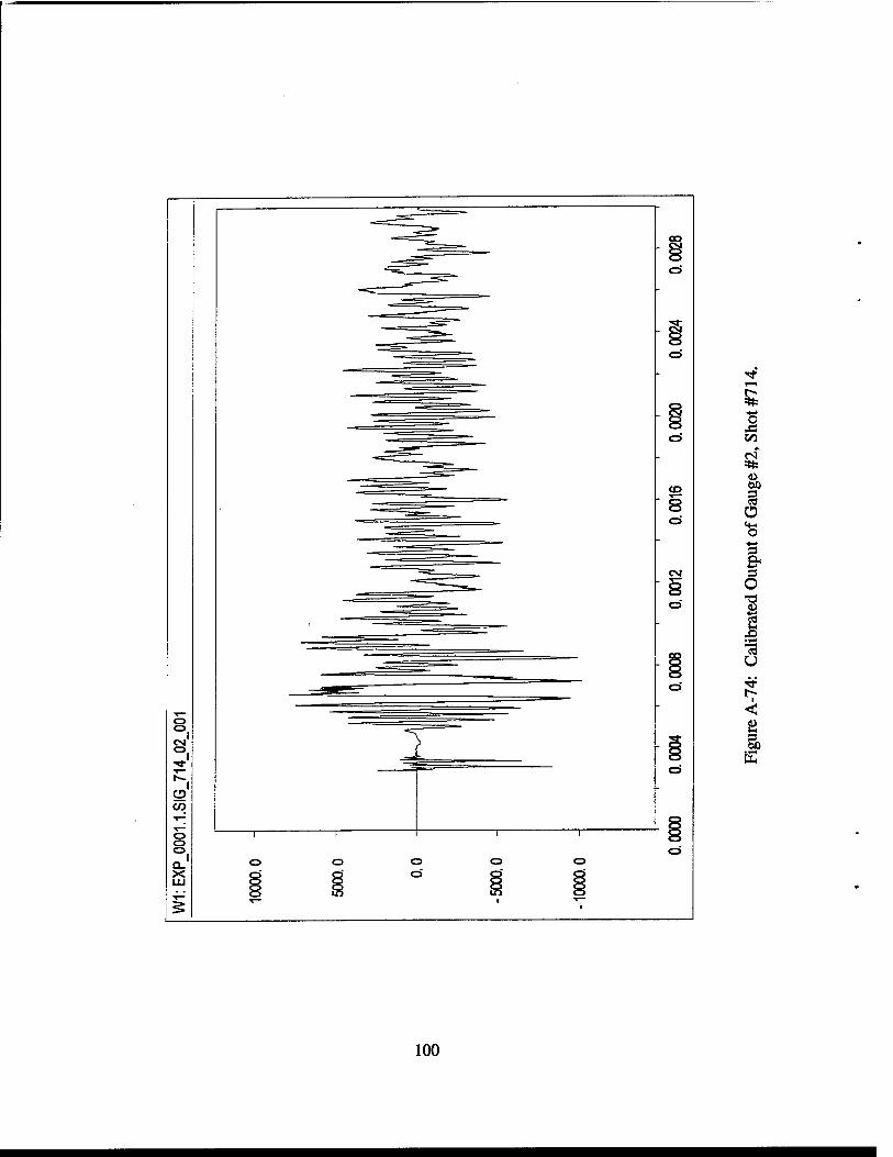
A-74 Calibrated Output of Gauge #2, Shot #714 100
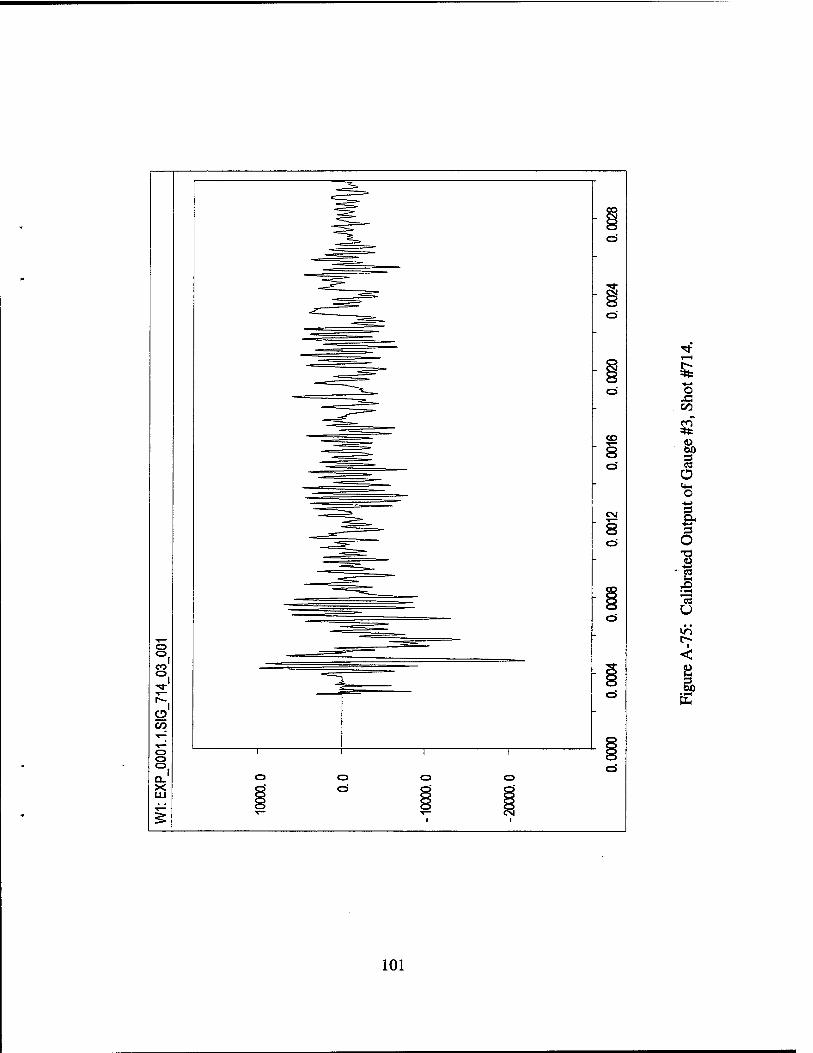
A-75 Calibrated Output of Gauge #3, Shot #714 101
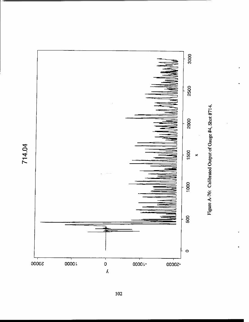
A-76 Calibrated Output of Gauge #4, Shot #714 102
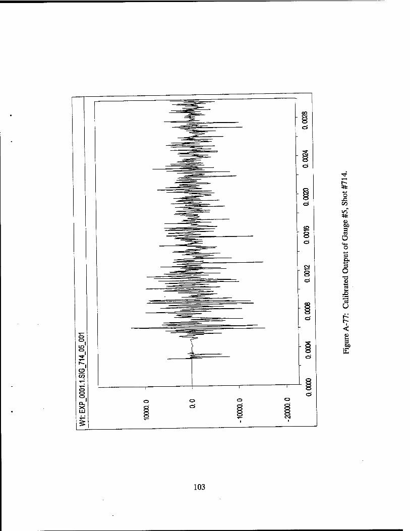
A-77 Calibrated Output of Gauge #5, Shot #714 103
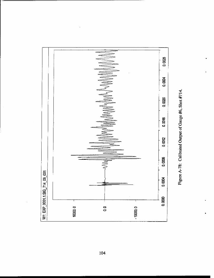
A-78 Calibrated Output of Gauge #6, Shot #714 104
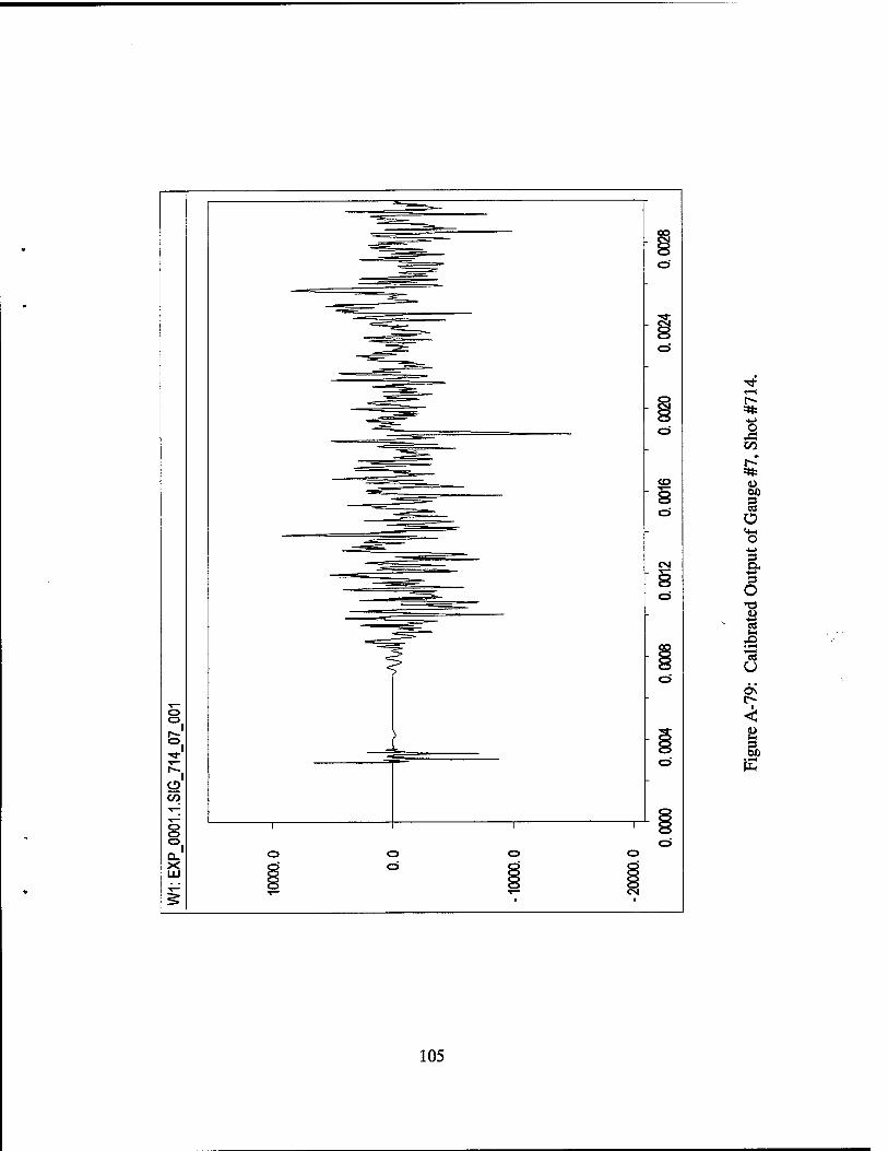
A-79 Calibrated Output of Gauge #7, Shot #714 105
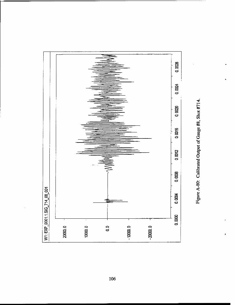
A-80 Calibrated Output of Gauge #8, Shot #714 106
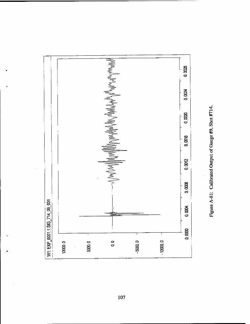
A-81 Calibrated Output of Gauge #9, Shot #714 107
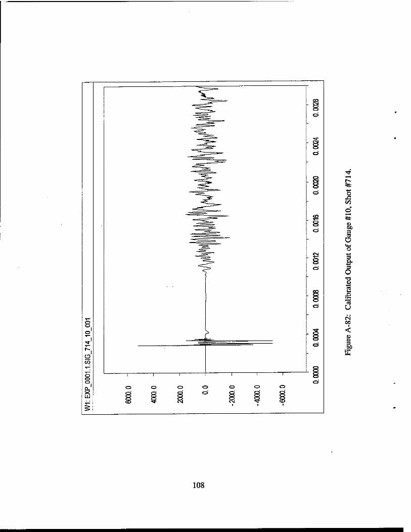
A-82 Calibrated Output of Gauge #10, Shot #714 108
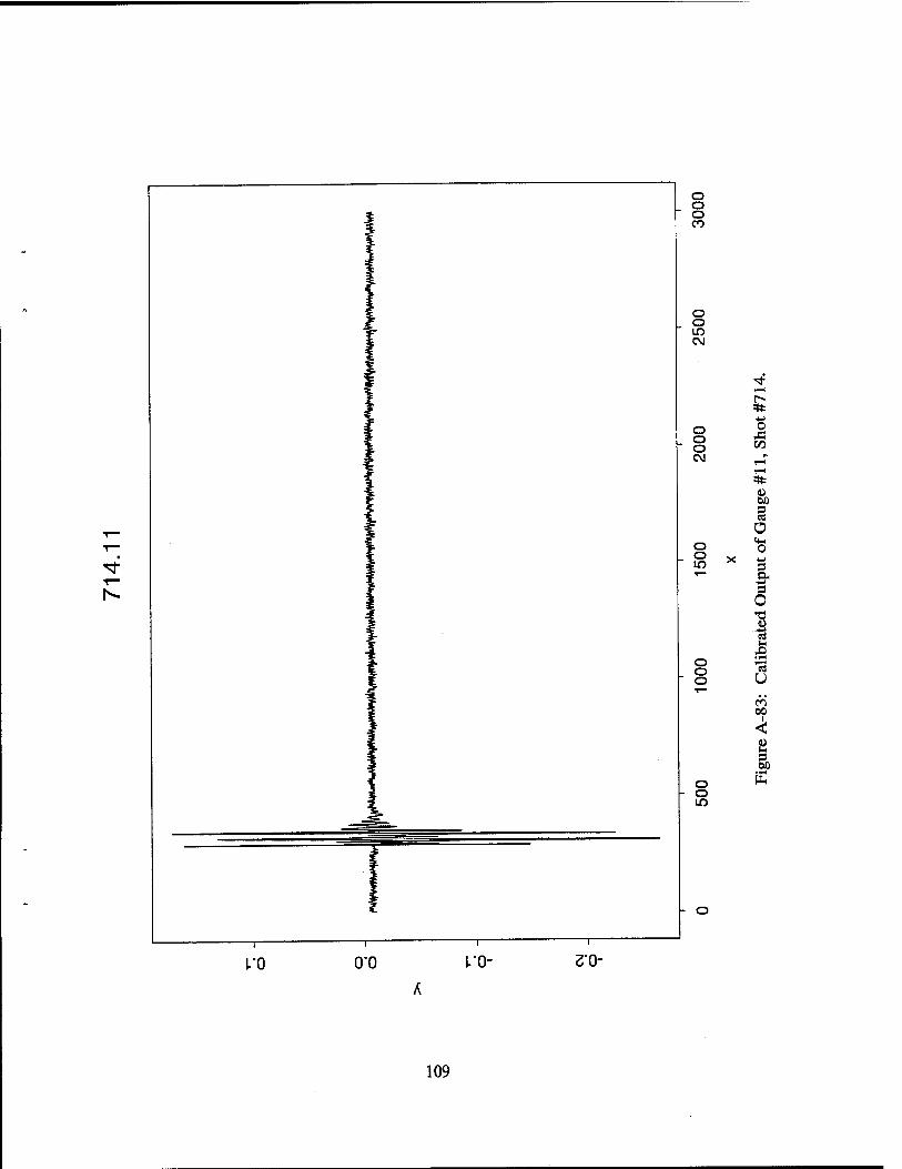
A-83 Calibrated Output of Gauge #11, Shot #714 109
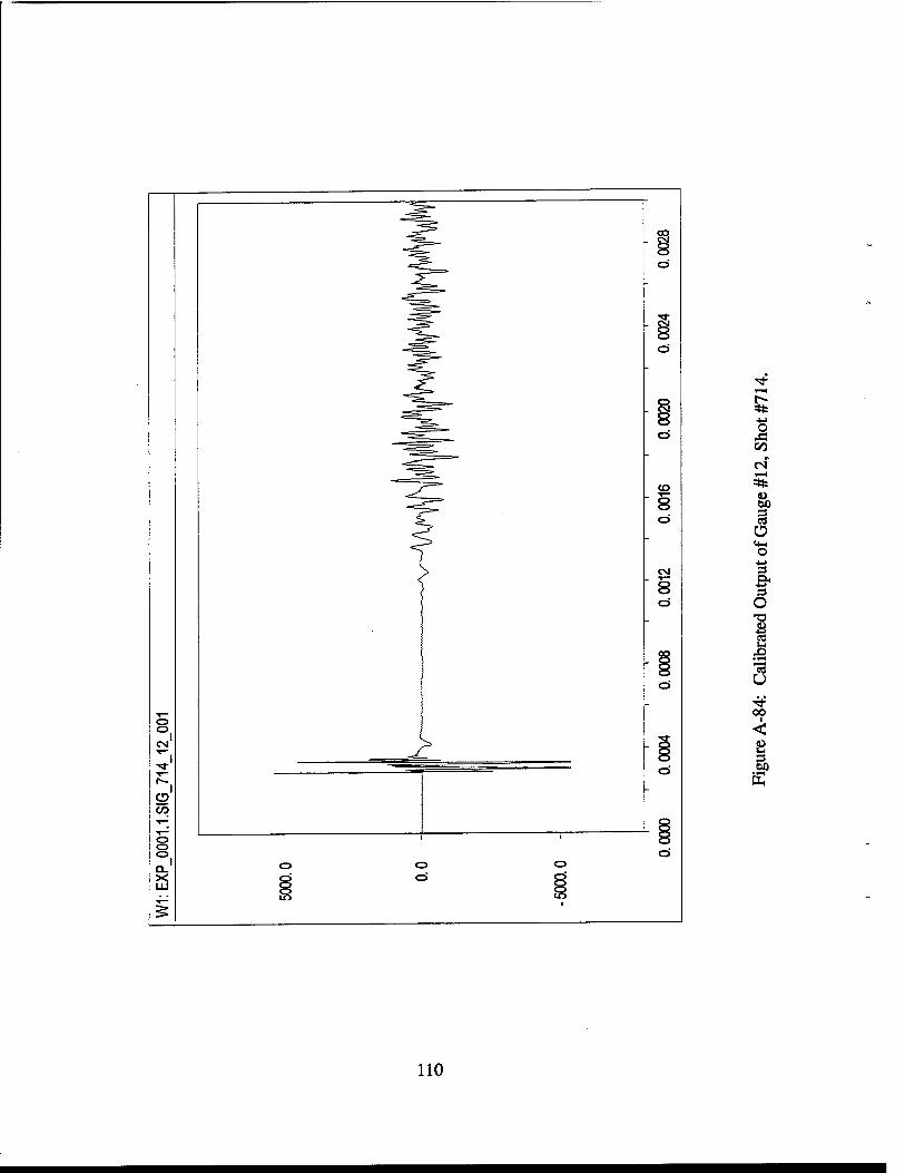
A-84 Calibrated Output of Gauge #12, Shot #714 110
A-85 Calibrated Output of Gauge #10, Shot #719, Position 1 . . . Ill
A-86 Calibrated Output of Gauge #12, Shot #719, Position 2 . . . 112
A-87 Calibrated Output of Gauge #9, Shot #719, Position 3 . . . . 113
A-88 Calibrated Output of Gauge #8, Shot #719, Position 4 . . . . 114
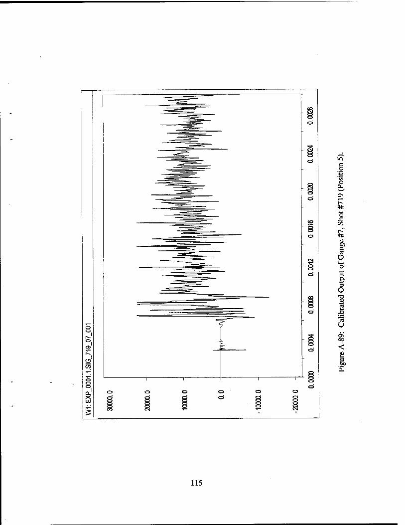
A-89 Calibrated Output of Gauge #7, Shot #719, Position 5 . . . . 115
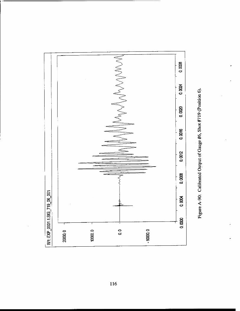
A-90 Calibrated Output of Gauge #6, Shot #719, Position 6 . . . . 116
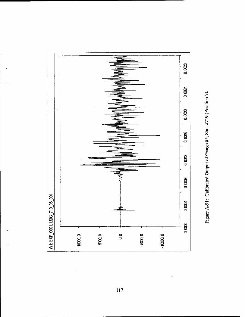
A-91 Calibrated Output of Gauge #5, Shot #719, Position 7 . . . . 117
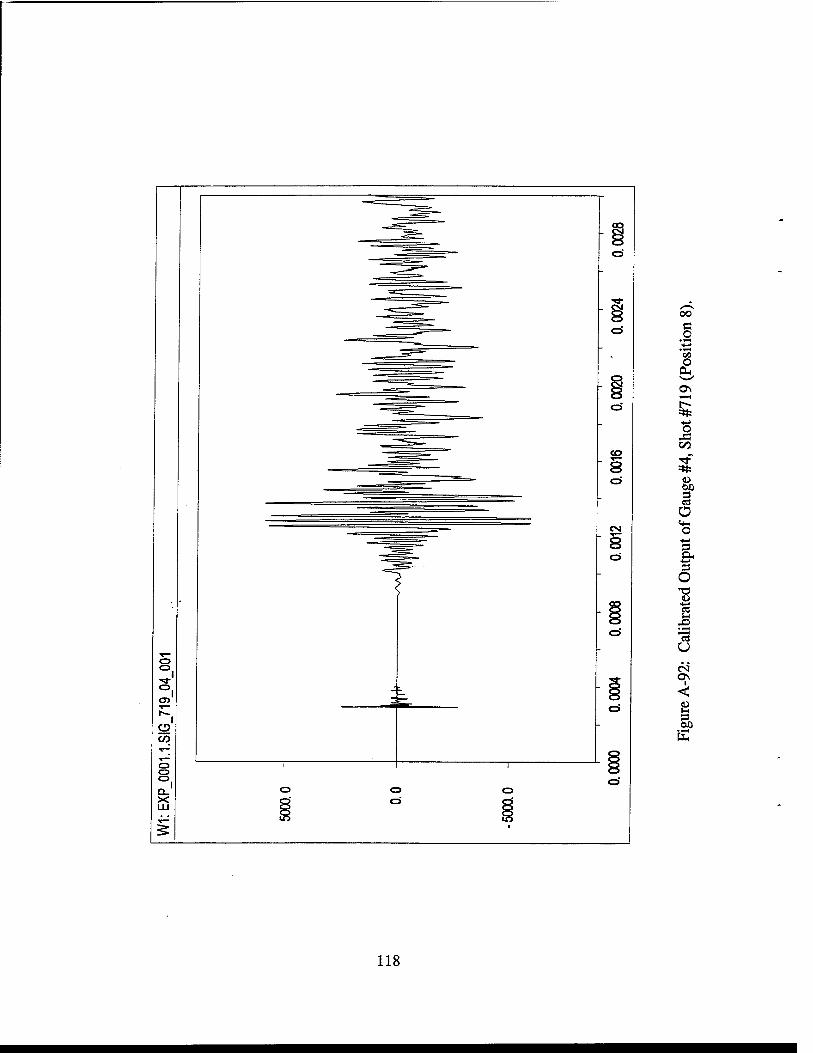
A-92 Calibrated Output of Gauge #4, Shot #719, Position 8 . . . . 118
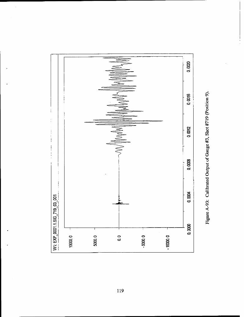
A-93 Calibrated Output of Gauge #3, Shot #719, Position 9 . . . . 119
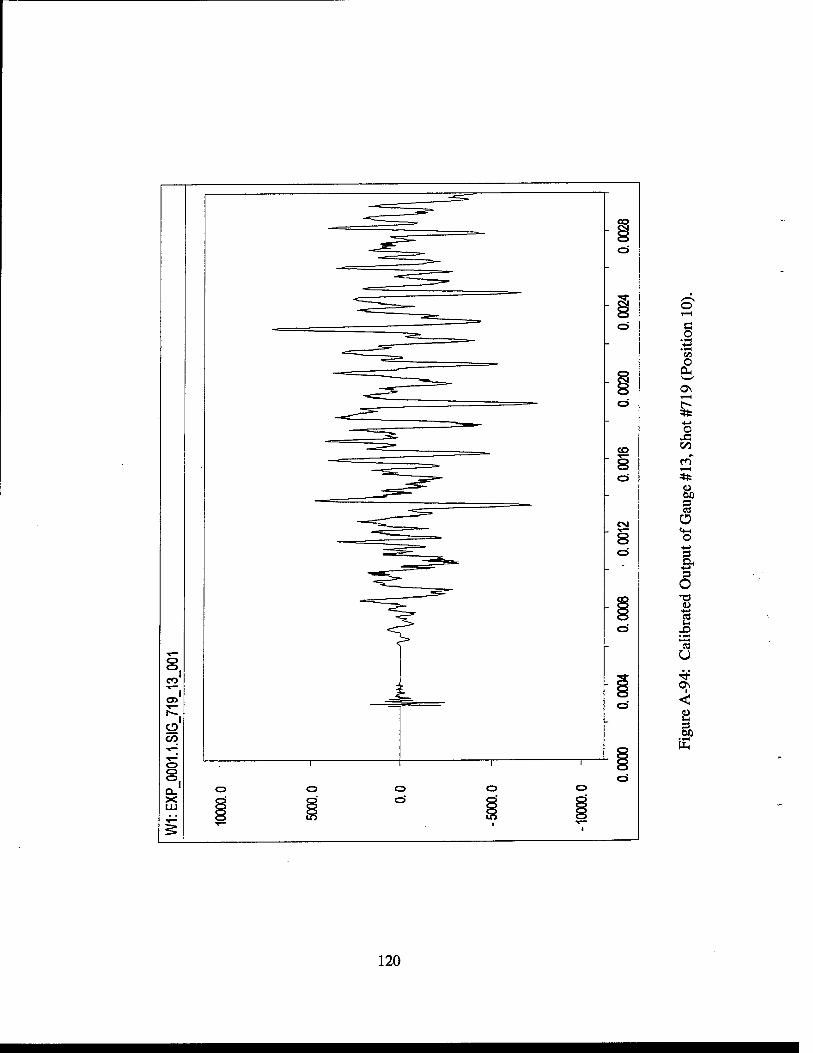
A-94 Calibrated Output of Gauge #13,. Shot #719, Position 10 . . . 120
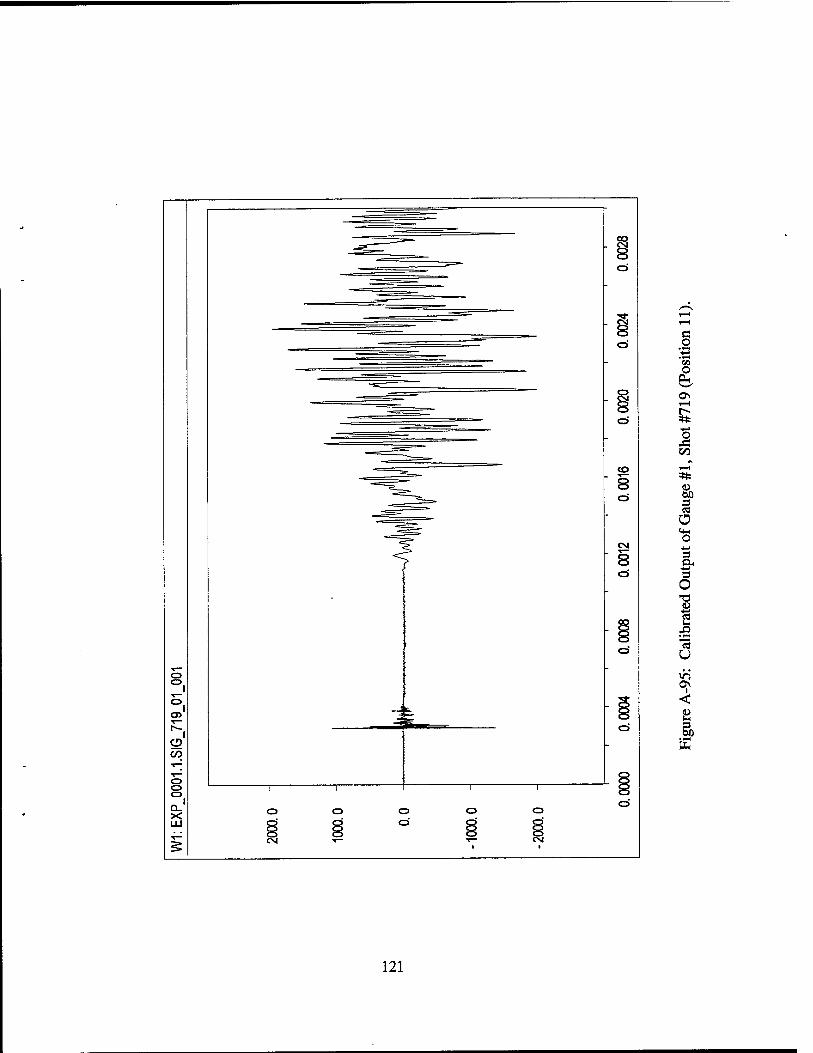
A-95 Calibrated Output of Gauge #1, Shot #719, Position 11 . . . 121
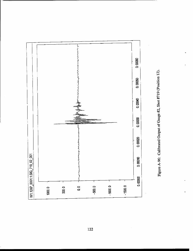
A-96 Calibrated Output of Gauge #2, Shot #719, Position 12 . . . 122
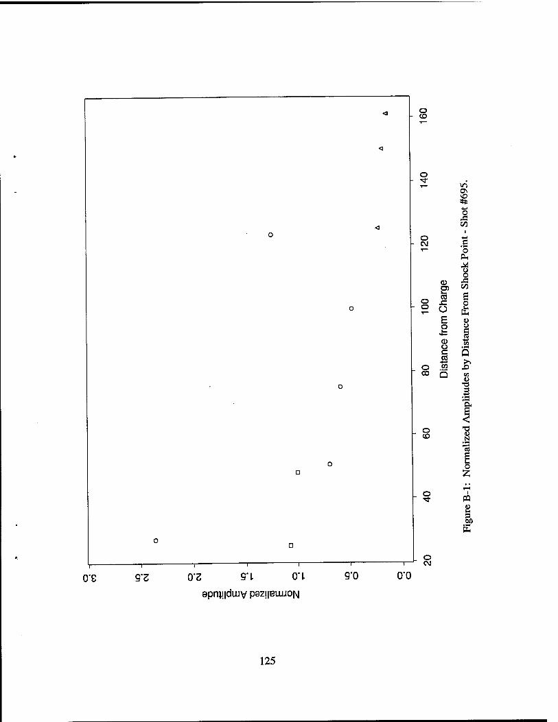
B-l Normalized Amplitudes by Distance from Shock Point - Shot #695 125
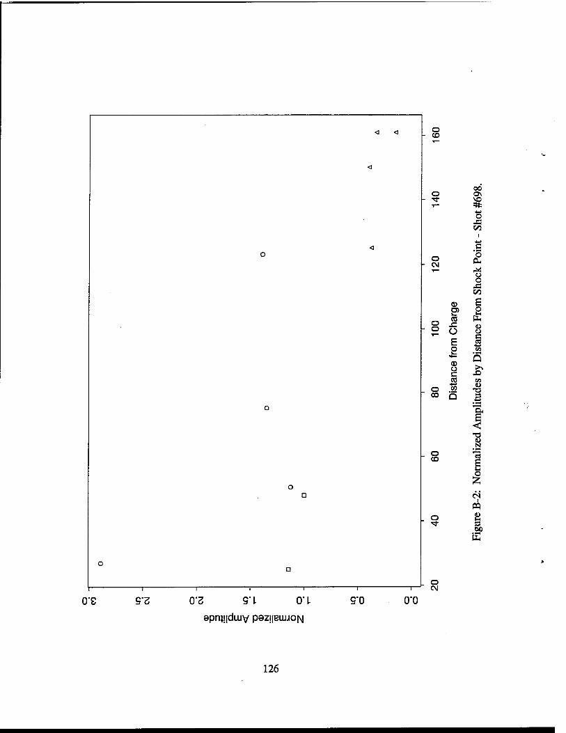
B-2 Normalized Amplitudes by Distance from Shock Point - Shot #698 126
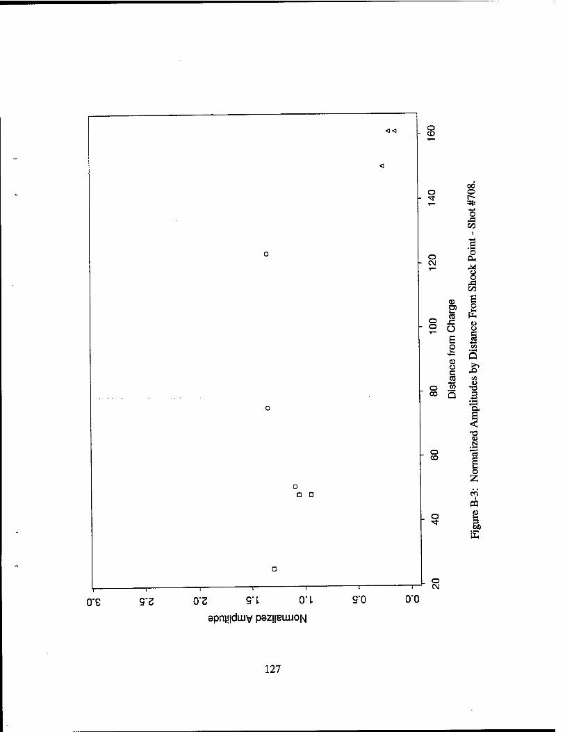
B-3 Normalized Amplitudes by Distance from Shock Point - Shot '#708 127
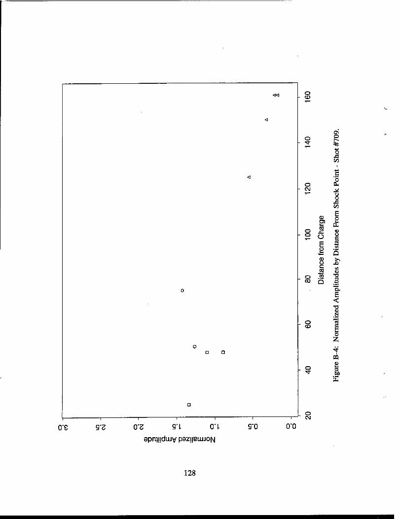
B-4 Normalized Amplitudes by Distance from Shock Point - Shot #709 128
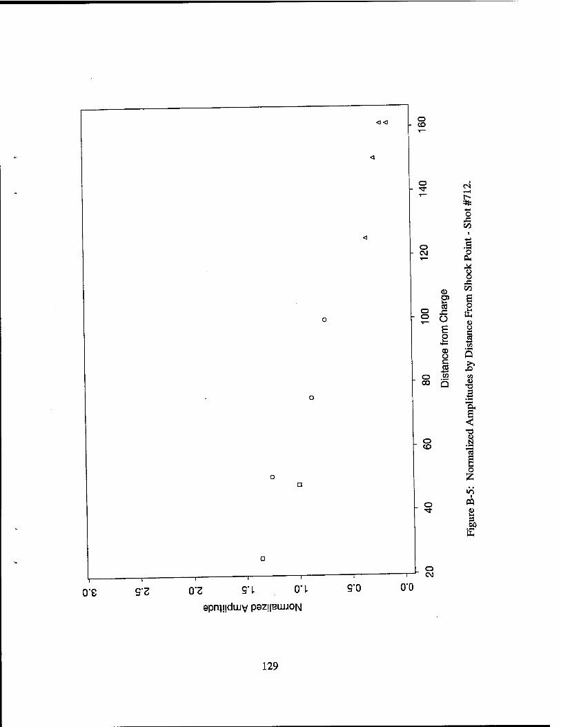
B-5 Normalized Amplitudes by Distance from Shock Point - Shot #712 129
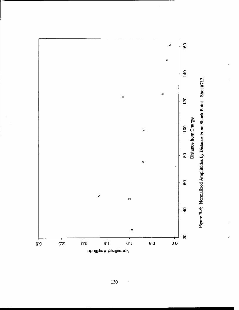
B-6 Normalized Amplitudes by Distance from Shock Point - Shot #713 • • 130
xi

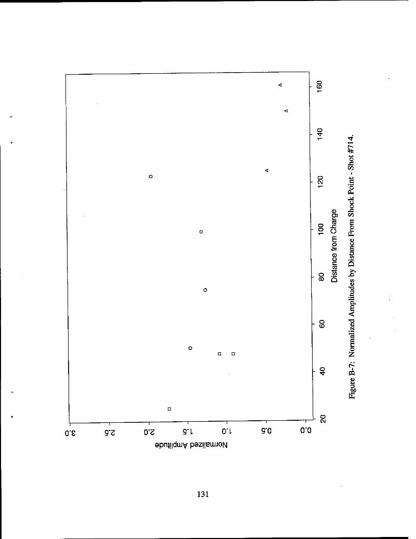
B-7 Normalized Amplitudes by Distance from Shock Point - Shot #714 131
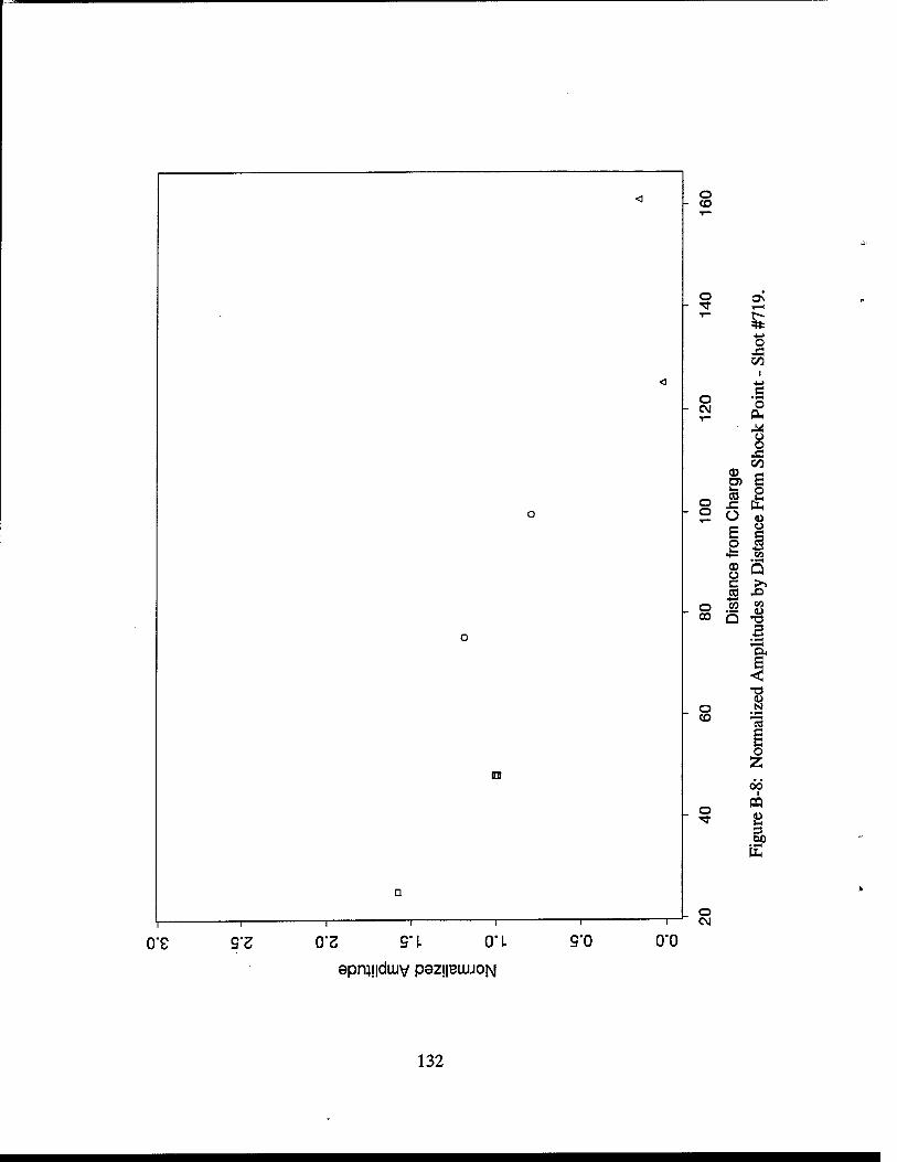
B-8 Normalized Amplitudes by Distance from Shock Point - Shot #719 132
Xll
List of Tables
1 Gauge Distances and Intervening Edges 3
2 Shot Numbers of Data Included in This Analysis 4
3 Data Removed from Analysis 15
xni

This page intentionally left blank
xiv
I. Introduction
When a significant amount of energy is deposited onto a small area (or into a small volume) of a structure, a physical phenomenon known as ballistic shock may occur. In this phenomenon, a portion of the deposited energy is transmit- ted away from the immediate region of deposition through the violent vibration of the structure. In the case of armored vehicles and other structures made of resilient materials, this energy may be transmitted (dispersed) throughout the structure including areas far removed from and not exposed to the incident agent. Thus, if transmitted to vibration-sensitive components, a system may undergo failure via damage that occurs far removed from the point of impact.
Note that this phenomenon can occur whether or not the incident agent (e.g., a kinetic energy penetrator or shaped charge jet) perforates the struc- ture.
For the balance of this discussion, we shall assume that the target is an armored vehicle which is struck on its integral, metallic hull.
Target response to ballistic shock is conveniently divided, by vibrational modes (and associated frequencies), into two markedly different physical domains. The lower frequency domain - up to approximately 1 kHz - is dominated by large-scale flexural vibrations, which include by far the majority of the en- ergy imparted by the incident agent. This is distinguished from the higher domain (above 1 kHz) by relatively larger deflections but relatively lower ac- celerations. As vibrational frequencies increase above 1 kHz, the dominant mechanism for the propagation of vibrational energy changes from flexural vi- bration of the system as a whole to stress waves in the material itself. It is not surprising, therefore, that the two domains manifest significantly different damage mechanisms. Energy in the lower frequency domain tends to produce structural damage, such as the failure of plates and edge joints (welds). In the higher frequency domain, the energy tends to produce damage of light, intricate, frequency-sensitive components such as electronics and optics.
This report deals exclusively with the measurement and analysis of ballistic shock in the higher frequency domain (above 1 kHz).
A salient characteristic was observed by Petty1 in experiments involving high- frequency ballistic shock. In measurements taken with accelerometers (see below), it was observed that the initial, transient, high-frequency pulse of
1 Petty, D. Private communication. U.S. Army Research Laboratory, Aberdeen Proving Ground, MD, 1997
energy that first reaches any given point inevitably included the highest of the high-frequency amplitudes. That is, in actual ballistic shock events, the leading (transient) pulse is always the strongest - and hence, presumably, the most damaging. Thus, it appears justified to confine the analysis of the higher frequency domain to this "leading edge". This simplification is important for two reasons. First, measurements of vibrations in the high-frequency domain are eventually overwhelmed by the large amplitude, low-frequency motions of the target. However, these low-frequency motions become apparent only after several milliseconds, by which time the high-frequency leading edge has passed and been recorded.
In addition, the ability to concentrate on the passage of the leading edge re- sults in a significantly simplified analysis. Rather than tracking all vibrations throughout a vehicle until all energy has been dissipated, it is reasonable to model the spread of high-frequency energy as a single wavefront that prop- agates outward from the source. (First-order corrections at boundaries are discussed in Section III.) This allows formulation of a linear model in which the propagation of energy from point to point is characterized by "transfer functions". Such a model is amenable to incorporation into the production- grade computer codes that are used for routine vulnerability analyses and the generation of large amounts of vulnerability data.
This report presents data, data analysis, and attempts at deriving a semi- empirical model of the high-frequency ballistic shock phenomenon. In this limited study, only one set of experiments on one relatively simple vehicle (Ml 13 armored personnel carrier) is presented. Other data taken by Petty and others remain to be fully analyzed. It is also recognized that newer vehicles, with composite and/or double hulls, will introduce further complications into this treatment. Application of the findings of this study to such cases is discussed in Section IV.
II. Experimental Procedure and Results
In the experiment analyzed herein, an Ml 13 armored personnel carrier (a ve- hicle with monolithic aluminum exterior walls and top) was instrumented as shown in Figures 1 and 2. Gauges consisted of single directional (perpendicular to mounting surface) accelerometers, made and calibrated by PCB Piezotron- ics, Inc. Advertised operating range was 0.1-20 kHz, with a rise time of 5 fis. All gauges were screwed into holes that had been drilled and tapped directly into the aluminum hull of the test vehicle. Outputs were digitally recorded.
In these experiments, the input shock was produced by detonating a bare charge of pentolite that was fixed to a 30.5-cm x 30.5-cm x 2.54-cm (12-in x 12-in x 1-in) aluminum plate (the "charge plate") mounted on the vehicle where shown in Figure 2. In all cases, the charge weight was 56.7 g (l/8th lb). Gauge distances from charge-center and number of intervening edges vs. gauge numbers are given in Table 1.
Table 1: Gauge Distances and Intervening Edges.
Gauge Distance (in.) Intervening No. from Charge Edges
1 48 0 2 48 0 3 25 0 4 27 5 50.5 6 75.1 7 99.6 8 123.1 9 125.1 2
10 150.1 2 11 161 2 12 161 2
The experimental series consisted of eight data shots herein referred to by their range sequence numbers, as given in Table 2.
Table 2: Shot Numbers of Data Included in This Analysis.
695 698 708 709 712 713 714 719
98 1/8"
© © © © © Gage8 Gage7 Gage6 Gage5 Gage4
-Hi" |*«-24 1/2"-*"
|*—491/16" ► 73 5/8" ►
971/8"-
Charge Side
Figure 1: Gauge Positions on Ml 13, Top View.
31"
• Gage 8 • Gage 7
• Gage6 • Gage5
* Gage4
' Gage3
30"
1 . | | 5" / Gagel
| \+— 48'!
Charge Side +
190"
• Gage 4 • Gage 5
• Gage6 • Gage7
* Gage8
Gage9
Opposite Side
/ Gagel 1 Gagel 0
Figure 2: Gauge Positions on Ml 13, Side Views.
The output of each gauge, scaled by its calibration, is presented in Appendix A. A typical plot, that of Gauge #6 in shot #709, is presented in Figure 3. The following characteristics are noted:
a. First, two ultrahigh frequency "spikes" riding on the initial quiescent signal.
b. After another quiescent period, a series of low-amplitude "ripples".
c. Then, a mass of high amplitude oscillations - in this case, at about 3 kHz.
d. Degradation into a more noisy appearing, lower amplitude signal.
e. Although not apparent in Figure 3, there is also the beginning of a longer time period baseline shift incorporated in the noisy tail of the plot.
o
o 00
=tfc Ü 60
o O <-> =3
e« =5 o i 1 U en 8 s bO
(SQ) uoi^japooy
7
III. Analysis
A. Extraction of Metrics.
1. Pulse Shape Analysis.
Analysis of the calibrated data traces resulted in the following conclusions. (Italicized terms are defined for use in subsequent discussions.)
First, the leading ultrahigh frequency spikes are caused by the trigger pulse, the electrical signal that initiated the detonation of the shock-producing charge. Since this pulse is simultaneously recorded on the output of every detector, this ultrahigh frequency spike can serve as a zero-time marker on every detector record.
Following detonation, there is a quiescent period at the detector sites dur- ing which the ballistic shock is forming and propagating outward from the shock point. The subsequent low-amplitude ripples indicate the arrival of a longitudinal vibration spreading out from the shock point through the vehicle hull. The speed of a longitudinal vibration is higher than that of a transverse one, explaining its early arrival. However, since the detectors were designed to respond to transverse vibrations, the amplitude of detector response to the longitudinal vibration is low. We refer to this set of early, low-amplitude ripples as the precursor pulse.
This is followed by the arrival of and detector response to the transverse vibra- tion, herein referred to as the main pulse. As reported by Petty, the response is most severe within the first few milliseconds: within ten ms, the amplitude has decreased significantly, with only isolated subsequent cycles reaching 20% of the highest peaks. This lower amplitude "noise" continues throughout the remainder of the measurement period.
Longer term data traces exhibit marked low-frequency rises and falls of the baseline on which this noise rides; these low-frequency oscillations are the response of the vehicle as a whole to the low-frequency portion of the shock.
Using this analysis of the characteristics of each detector output, it was possible to define and extract metrics that characterize the data of interest for this study.
2. Arrival Time Analysis.
First, in order to verify the above analysis, it was illustrative to extract from each data record the times between the trigger pulse, the arrival of the first low-amplitude oscillation, and the arrival of the first high amplitude oscilla- tion. To do this, a computer program was written that distinguished signals above appropriate thresholds, sensed frequency by the number of consecutive readings above threshold, and counted data points in the intervals. From this two sets of timing data were extracted: trigger-pulse-to-arrival-time for the precursor pulse (Tl data) and trigger-pulse-to-arrival-time for the main pulse (T2 data).
Analysis of these data follows. In this analysis and all that follow, functions were fit to the data using the S-PLUSt statistical software analysis package.
First, from a plot of the Tl data for the gauges on top of the Ml 13 (top gauges) vs. distance from the charge point (Figure 4), the precursor pulse speed can be calculated. Fitting the Tl data with a straight line yields a slope of 0.20 in/fis which equates to a speed of 5080 m/s, somewhat less than the published speed2 of a longitudinal wave in bulk rolled aluminum (6420 m/s), but slightly greater than the speed of a longitudinal wave in an aluminum rod (5000 m/s) which, as in the present case, exhibits boundary effects upon wave speed. We conclude that the measured speed is consistent with the existence of a iongitudinal wave.
Similarly, a plot of the T2 data for the top gauges (Figure 5) yields a slope of 0.12 in//zs which equates to a speed of 3055 m/s, in excellent agreement with the published value of a transverse wave in rolled aluminum (3040 m/s).
We conclude that the observed data traces are caused by the arrival of a longitudinal disturbance followed by a transverse one.
In the analysis of the T2 data, a phenomenon was noted which gave important guidance to the amplitude analyses presented in the next section of this report. A plot of T2 data that includes both the front surface and the top surface reveals an interesting paradox. As seen in Figure 6, the arrival of the transverse pulse at points on the top surface actually occurs before the arrival of the pulse at equal distances on the front surface - even though the pulse arriving at the
tS-PLUS is a software product of Statistical Sciences, Inc., 1700 Westlake Ave. N.,Suite 500, Seattle, WA 98109.
2 Handbook of Chemistry and Physics, Forty-Fourth Edition, Chemical Rubber Publishing Company, Cleveland, OH, 1963.
200 400 600 800 t(usec.)
Figure 4: Arrival Time of Precursor Pulse - Top Gauges.
Figure 5: Arrival Time of Main Pulse - Top Gauges.
10
top points must negotiate the intervening edge. From the intercepts of the two lines plotted in -Figure 6, the time difference is found to be 67 //s.
o CM -
ooo
o a>oo/ o
o
Front Side Data Top Data
o -
o . CO
a cy 'CD CD
o _ to
o tar oo ..■■' a a
o .
D Ofl i ns' a
200 400 600
t(usec)
800 1000
Figure 6: Arrival Time of Main Pulse - Front and Top Gauges.
Analysis led to the following explanation. Detonation of the charge results in the creation of both longitudinal and transverse disturbances on the front side which propagate outward from the edge of the charge plate, with the longitudinal disturbance traveling faster as indicated above. Upon reaching the edge, the longitudinal disturbance generates both a longitudinal and a transverse disturbance on the top side (as well as reflected disturbances on the front). It is this transverse disturbance on the top surface, created by the longitudinal disturbance on the front, that first reaches the top surface gauges.
For this explanation to hold true, the difference between the time of arrival of the longitudinal disturbance at the top edge and the time for a transverse disturbance to travel the same distance - approximately 50.8 cm (20 in) - must account for the time difference noted in Figure 6. Using the speeds measured from Figures 4 and 5, we find
Time Difference = 20
0.12 20
0.20 = 67 fis
11
in remarkable agreement with the 67 //s measured in Figure 6.
We conclude that the initial portion (approximately 70 fxs) of the transverse vibrations measured on the top surface is generated at the intervening edge by the arrival of the longitudinal disturbance on the front side. As shown below, this conclusion dictates the form of the functions used to fit the amplitude data in Section 4.
3. Amplitude Metrics.
Inspection of the calibrated data traces (Appendix A) reveals a great deal of chaos in the high-frequency vibration record, as is to be expected in a shock environment. In order to characterize the amplitude of each trace in a consistent manner, the following technique was used.
First, visual analysis of the data traces was made. This analysis identified and removed those traces in which obvious experimental difficulties were experi- enced. For example, the data trace for Gauge #4 in Shot #713 (Figure 7) is clearly oversaturated, as - somewhat more subtly - is the same gauge in Shot #708 (Figure 8). (The behavior of Gauge #4 in general is discussed below.) The data so removed are listed in Table 3.
A utility code was written to conduct the data extraction. Operating on the complete files of calibrated data, this code removed the data listed in Table 3, extracted the arrival times presented in the preceding section, and also performed amplitude characterization. This characterization consisted of identifying peaks in each data trace by comparing the values of adjacent data points. For each trace, peak amplitudes were then tabulated. In order to "smooth out" the chaos evident in the traces, the N highest peaks were then averaged. Clearly, larger values of N tend to give smoother data, but also dilute the differences between gauge outputs. After trying several values of N, it was decided to characterize the output of each gauge for each shot by the average of the four highest peaks in the corresponding data trace. We refer to these averages as the "top4" metric. Thus, the magnitude of the shock measured by each gauge for each shot is represented by a single top4 number.
It was recognized that, in order to include data from different shots into a single analysis, it would be necessary to normalize all data records to remove shot-to-shot variations. Thus, as a final step in the extraction of top4 data, all top4 numbers from each shot were normalized. Two normalization schemes were investigated. In the first scheme, each top4 value for each gauge for a given shot was normalized to the average of the top4 numbers of all gauges
12
o o o CO
o o IT) CM
(T5 o ^H
o p- o * CM ■4->
o X! CO
CO *t
O Ö o Ü 3 O
ID CD CO O o <+-i S-l o
•l-H 4-> 3 & 3 o 13
O 1 o o x>
U
e o tu o ir>
00003 00002-
13
00 o
t CO
o 00
3 ü
o 1 I U öd s s
(SQ) uoi^-BJapoov
14
Table 3: Data Removed from Analysis.
Shot # Gauge # 695 1 698 1 698 7 708 4 708 7 708 9 709 4 709 7 709 8 712 4 712 8 713 4 713 11 714 4 714 11 719 2 719 7 719 8 719 11
15
for that shot. The second scheme used the output of only the distant front- face gauges (gauges #1 and #2) as the normalization constant for each shot. Since the second scheme was found to introduce less scatter into the data than the first, the analyses reported below were done using data normalized by use of the second scheme. Note that normalization loses any information on the absolute acceleration of any point, which was not of interest in this study. Preserved is the relative acceleration of each point with respect to that of the other points for that shot. This normalization allowed data from the eight shots listed in Table 2 to be combined into a single analysis even though experimental vagaries resulted in different initial shock levels for the various shots.
A utility code then gathered the normalized numbers, associated them with the corresponding distances from the shock point and numbers of interven- ing edges, and formed matrices for the analysis presented in the next section. A plot of the combined normalized data, by distance from the shock point, is presented in Figure 9. Similar plots, containing the normalized data from each shot individually, are presented in Appendix B. In these plots, squares repre- sent data from front face gauges, circles from top face gauges, and triangles from rear face gauges.
Recall that there were two gauges on the front face at 48 in from the charge, the average of which was used to normalize all data from a particular shot. This averaging accounts for the spread in the points at 48 in from the charge. Had there only been one gauge at 48 in, all points at that abscissa would fall exactly at a normalized amplitude of 1, of course.
4. Semi-empirical Equation Development.
The approach taken to fitting the Ml 13 ballistic shock data in Figure 9 was to hypothesize various physical phenomena which could be important in the propagation of the leading edge of the high-frequency shock wave to the various gauges over the vehicle. The expected behavior of each of these phenomena was parameterized and included in a comprehensive function which was then fit to the data. This resulted in the systematic set of progressively more complex semi-empirical fits. Goodness of fit was assessed via the residual sum of squares calculated by the S-PLUS statistical software analysis package.
In this section, we present the final equation used to fit the data in Figure 9.
Modeling of the following physical phenomena effected the best fit:
16
«
< <<wa
< < «i « < oo o o
ooo o
o o o o o o o
O O O CD O
D D ODD DD D
o CO
o ^- T—
.s
O ■8 o CM T—
I © PH O) u CO u o £Z s o O B
OS
E o Q k. >> <D
Xi Ü C co ■8
5 o CO CO Q OH
1 o ON CD
8
o ■^r
o CM
0-8 9'2 0'3 9'I. OH
apnijiduuv pazpuuoN
9'0 0"0
17
•
•
•
•
The existence of two wave modes, longitudinal and transverse, denoted by subscripts 1 and 2, respectively.
The mixing of modes, as modeled by parameters Cij,i, j = 1, 2.
Mode-dependent exponential decrease in amplitude with distance.
Amplitude enhancements at points close to an edge, with differentiation between points before an edge (subsequent edge) and points beyond an edge (preceding edges) (as viewed from the source).
The resulting equation can be succinctly written as follows.
Yi = At x e"**-* x (1 + D x e~d-r) x (1 + F x e~f-s) (1)
A{ (new face) = dj x Yj (edge of preceding face)
where
Yi = Amplitude of the disturbance i = Subscript indicating longitudinal (1) or transverse (2) A,- = Amplitude at charge point/each succeeding edge b; = Decrease with distance (exponential parameter) x = Distance from charge point to measurement point D = Enhancement due to proximity of subsequent edge d = Decrease in D with distance from subsequent edge r = Distance from subsequent edge F = Enhancement due to proximity of preceding edge f = Decrease in F with distance from preceding edge s = Distance from preceding edge
The ability of Equation 1 to fit the Figure 9 data is shown in Figure 10. The data set consists of 75 points. However, it must be pointed out that the available data were not sufficient to determine all of the above parameters. For example, the Cy were found to be irresolvable. Two Cy could be freed to fit to the data only if the A, were fixed; however, attempts to free both the A; and Cy or to free more than two Cy led to "singular gradient matrix" errors in the fitting routine, an indication that the fitting parameters are not independent with respect to the available data. Similarly, it must be noted that the value of A2 was effectively set by normalizing to a front face point. Hence, in the actual fitting equation, there were six free (fitting) parameters, viz:
18
o CD
O 'S-
o CM
0
° o
o CD
o
E p
CD Ü C « to o ._
CO Q
O CM
ere 9'2 O'S 9" i. OH
apnjiidujv pezi|BUJJON
.S o AH
4= CO
1 o
CO
•a
to
K
Ö s
19
Ai - Amplitude at charge point/each succeeding edge bi - Decrease with distance (exponential parameter) b2 - Decrease with distance (exponential parameter) D - Enhancement due to proximity of subsequent edge d - Decrease in D with distance from subsequent edge F - Enhancement due to proximity of preceding edge
Goodness of Fit.
Evaluation of the goodness of fit of a non-linear equation is generally prob- lematic. However, the following technique, adopted from Draper and Smith3
provides a reasonable (practical) measure. Effectively, the technique compares the intrinsic scatter in the data from their means to the scatter of the data from the fit at each measurement point.
Note that the technique for estimating intrinsic scatter requires more than one independent measurement be taken at some or all of the measurement points, a condition assured from the beginning in this analysis by combining the (nor- malized) data from the eight shots listed in Table 2. (See Section III.A.3.)
The intrinsic scatter is characterized as follows: The "pure error sum of squares", S2, in a data set containing more than one value at each point in the independent variables, is defined as
E E (Ykj ~ Yh)\ (2) k=l j=l
where rik are the number of values at each of K measurement points, Ykj are the data and Yk are the means at each measurement point. Since K means have been computed, the total degrees of freedom in computing S2 is given by N-K, where N is the total number of data. Thus, the "mean square for pure error" is given by
2 _ Ef=i E£i (Ykj - Yhf Se N-K (3)
3Draper, N. R., and H. Smith. Applied Regression Analysis. New York: John Wiley k Sons, Inc., 1966
20
The scatter of the data from the fit is characterized by
N
= EW M (4) t=l
where Y{ is the fitted value corresponding to the iih datum. The number of degrees of freedom in S2 is the number of data, N, minus the number of fitting parameters, m, in the equation for S2. Thus, the mean square scatter of the data from the fit is given by
*; = N — m (5)
For the data in this analysis, we find
Parameter Value Statistic Value
N 75 s2 3.00035
m 6 4 0.04616 K 10 s2
3.08613
«2 0.04473
Note that si is less than s\.
Heuristically, one can think of this goodness of fit analysis as follows. In ad- dition to the underlying physical phenomena which we wish to model, the data contain indeterminate contributions ("pure error") from experimental vagaries, measurement error, and other sources. We assume that the indeter- minate contributions are randomly distributed about the mean at each mea- surement point and therefore that the mean at each measurement point is the best estimate of the true value at that point. The fit (Equation 1) attempts to produce the true values via a parametric equation. We therefore ask to what
21
degree does the intrinsic scatter of the data about each best estimate compare to the scatter about the fitted value.
Bodt4 notes that the complexities in nonlinear modeling do not support the same statistical tests that linear modeling supports. However, similar test constructions as in the linear case are still often used, but with the caveat that the actual distribution of the test statistic is unknown.
Even with that caveat, Bodt points out that the use of the F-statistic to compare si and si would be unwarranted. An F random variable is the ratio of two independent Chi-Square random variables. But, the Chi-Square variate based on the residual mean square (si) and the Chi-Square variate based on the pure error mean square (si) are not independent.
However, the Chi-Square variate based on the residual mean square with the pure error mean square removed is independent of the Chi-Square variate based on the pure error mean square. In this spirit, Draper and Smith suggest the following statistic to gain "an approximate idea of possible lack of fit":
(S2 - S2)/(K - m) nARA, .,. GoF s SV{N-K) = °-4645 (6)
which they compare to
F(K-m,N-K,0.95) « 2.5 » GoF.
The comparison here is significantly better than the example which, according to Draper and Smith,3 "would make us tentatively feel that the model does not fit badly". We thus conclude that Equation 1 accounts very well for the non-random behavior of the data.
4Bodt, Barry A., Private communication. U.S. Army Research Laboratory, APG, MD, 1997
3Draper, N. R., and H. Smith. Applied Regression Analysis. New York: John Wiley k, Sons, Inc., 1966
22
IV. Summary and Discussion
This study has dealt with the propagation of only the leading, high-frequency edge of the shock wave emanating from an impact point on an armored vehicle. Since the data show that this leading edge invariably contains the highest amplitude disturbances in the frequency range of interest, concentration on this phenomenon is warranted. Specifically, this study has analyzed the data taken in an experiment in which the vehicle was an M113 armored personnel carrier and the mechanism of shock production was an explosive charge placed on a striker plate which was in contact with the hull of the Ml 13.
This study has shown that the amplitude of the transverse wave can be well fit by a semi-empirical equation (Equation 1) which accounts for both a lon- gitudinal and a transverse wave, exponential decrease with distance, mixing of waves at edges, and amplification at points near edges. Since this analysis dealt only with the propagation of the leading edge of longitudinal and trans- verse disturbances within the hull material itself, the flexural response of the system as a whole was irrelevant.
Comparison of the leading edge velocities with data published for rolled alu- minum confirms the analysis of longitudinal and transverse disturbances. No further attempt was made to relate the results to material properties. At- tempts to do so will require data taken on structures made of other materials. Similarly, resolution of certain semi-empirical parameters, such as the mode mixing ratios, will require additional data from experiments specifically de- signed for such measurements.
It is seen that Equation 1 constitutes an algorithm that is suitable for incor- poration into vulnerability analysis codes. Such a code must propagate both the longitudinal and transverse waves through the hull material from point of impact to point of interest. At each intervening edge, amplitudes must be calculated for use as starting values for propagation on the succeeding face.
It is recognized that the above algorithm addresses only one of the three ma- jor factors in the analysis of the high-frequency portion of ballistic shock. Significant work is required on shock generation upon impact and upon com- ponent failure due to high frequency acceleration before a useful ballistic shock methodology can be assembled.
It is also recognized that newer vehicles, with composite and/or double hulls, will introduce further complications into this treatment. However, the results presented herein give a reasonable starting point for future development.
23

This page intentionally left blank
24
Appendix A
Calibrated Data
25

This page intentionally left blank
26
»n ON
CO
Ü 4-1 o 3
•a i In
u
8 s 60
27
m as \o *t +J o CO
u
Ü
3 s- 3 o
u
<
3
E
28
m ON }P =tfc *J o xi CO
CO
W)
Ü 'S
f o
i *e3 U
en i
s (90
29
m ON «5
■*-*
o
o
Ü
*-> 3 & s O
2
u
2
30
«n ON
* O
CO
«n
Ü o *-> 3 & S O
CS
U
i
s
31
ON VO *fc -4-1 o
iS <o 60
Ü <w o
S- 3 o
1 'S u VO
2
IS
32
ON
=8= *J O Ä CO
3 & a O
1 1 • PH
•a u
8 3
33
in ON
* <4->
o CO
00
o bo g Ü
s & s O
1 | 73 U
oo
s
34
ON v£> *: *-> O
C/3
bo
Ü 'S *->
o
x>
U
ON
8 s bO
35
«n ON VO
00
o o s & o
1 .•S 73 U
8 s 60
36
C/5
U
u o o +->
s O
2 •O
U
2 s
37
«n ON VO
o
St <D
Ü
a
o
I I "e3 u
2 3 00
38
o o o in
o o o ■■3-
00
g o
JS
o o o CO
00
CD o o o CM
00008 00009 000017
A
00002
o o o
o oo
O o
■4-J s & s O
I U CO
s 3» E
- o
39
00 ON \o =8: +■> O m
o o
I O
1 I U
8
40
00 <7\ VO
.§ CO
bo 3 o o s
o
i I u >n
s a E
41
00 as
£ o
CO
Ü o 13 & 3 o
1 1 u ^o
3
42
00 ON vo
■s CO
If? =tfc
1>
o 'S
s o
1 1 "3 U
2
E
43
00 C\ VO =*fc *-> o
CO
bo
Ü
s- s o
i i 'S U oo
8
44
o cd CO
o o o to
o o o "3-
o o o CO
o o o CM
o o o
00
g o
ü
i o
1 I ON
8
E
0000 L 0009 00001.-
45
00 ON VO =8= *J O Ä CO
oo
u
Ü
s s O
I 1 'S u
8
E
46
00 ON
Ü o
■*->
S & o
I u
i
< 8 S)
47
00 ON NO
CO
Ü
s
o
1 rS 13 U
8 3
48
00 ON VO
O
to
o 4-1 O
s & s O
• IM
'S u en
8 s 00
E
49
00 ON
$ o
43 </3
4)
Ü 'S
I 3 O
I U Tt cs
ß s
50
00 o
o Xi
3 ü
3 & 3 o
i i u
8 3> E
51
00 o & o
C/3
a
Ü
3 & S O
1 I u vö (N
8 s E
52
00 o
■4-1
en =tfc
&
Ü «4-1 o
& a O
2
U
55
8 a (90
53
00 o & 4-» o CO
"*" O
% o o
i- o
1 I "öS u oo
2
EE
54
00 O
Xi CO
«n
60 u o 'S 3 & o
1 I *c3 U
d\ cs
55
00 o
o X! Vi
so =tfc
8) % Ü 'S
i. o
I U © en
8 s E
56
o od o
o o o in
o o o
o o o CO
o o o CM
o o o
00 o & o
V}
u O o
% s O
1 I U
■ < 8 S) E
00002
57
00 o
o Ä VX
00
u 60
3 ü «4-1
O
3 & a O •o a CO
en
2 So
58
00 o
■M o
<u
s
o
I -t-H
■a u
3. E
59
00 o
XI CO
Ü
13
o -a
U
CO
8
60
00 o
o Xi CO
=tfc l>
I- o
'S u in en
8 3
61
00 o
X XA
ci »—I
60
Ü
f. 3 O
I u vö CO
i < s DO
62
ON o
o 00
to
a
s. 3 o
1 U «> en
8 s
63
ON o
o CO
Ü
s O
i I U
64
o
o A CO
u 00
a tu o +-J
& 3 o
1 2 X) 'S U ON
8
65
ON
S ■*-< o CO
ID
Ü (4-1 o
& 3 o
i 1 u
3»
66
O
o
O 4-1 o 3
a O
■I
U
< 8 §>
67
©
O ja GO
vo =tt i)
Ü «4-1 o s 3 O T3
1 U
S
8
E
68
o o
o o o
o o o «3-
o o o 00
o o o CM
o o o
o
CO
o o
■>->
3
s o
I "3 u 5?
8 s
- o
0009 00001-
69
ON o
o CO
00 =tt ID
O o
■4-J
s 3 o
I U
#'
2 s
70
OS ©
CO
Ü
s
o
1 "3 U
3
8
71
ON o
o CO
0)
s 3 o
I u
8 s 60
72
ON o
■4-* o Vi
•s & 3 o
I "öS u
8 3
73
ON o & o
VI
(N 1—1
Ü •s s B- s O
1 I • 1—1
U IX
8 60
74
*-> O Ä CO
=tfc u
Ü
& o
i 1 u §
2 s E
75
o CO
O o *-» 3 & S O
i 1 'S u o
76
es 1—I r»
o J3 CO
CO
bo
Ü 'S 3 & 3 o
•o u
1 'S ü
E
77
+^ O
X! co
=** m DO
Ü <4-l o ■*->
3 £< 3 o
|
u
8
E
78
es
o ja Ui
)D *: O ÖD
§ Ü «4-1 o ■4-1 13
3 O
1 I U
8
E
79
es 1—1
=tfc
o CO
&
O <** o ■4-J
3 & 3 o
I u
8
E
80
es r—I
si C/2
Ü o 4-1
l s O
i iS T3 U
8
81
es
s ■*-> o CO
oo <u
Ü o 3 & a O
I "03 u
ß
E
82
es i—i
o CO
ü
3 Ü
4-»
& s O
i 1-4
'S T3 U
8
83
es 1—1
o CO
O 4-1 o •4-» 3 & 3 O
I U
2 s
84
T—<
o Ä CO
o bo
Ü
'S
!■
o
"3 U ON
2 s
85
o GO
0) 60
Ü «4-1 o s
s O
I 'S U
o
8 s
E
86
en
o CO
=8= <L>
Ü o s & s O
1 I "3 U
< 8
87
CO 1—I
+-> o
u o o s & a O
1 a u
8
88
r-H
o CO
en =«: <U
Ü
3
o
1 u en
2 3 00
89
o CO
P3
o o o CO
o o m CO
o o o CM
o o m
o o o
o o to
CO
u
Ü o
I s O
I ä Ü 4c"
8
- o
OOOOS 00001 ooooi- oooos-
90
o CO
ID =tfc 0)
Ü o *■>
3 e* s O
1 J U
8
91
CO T-H
o CO
u
Ü
3 ß- 3 o
1 1 U
v©
•fi
92
■4->
O
l>
ID
O <4-l o
& s O
1 I U
ß s
93
£ o
VI
00
Ü 4-1 o
& 3 o
1 I 'a U
c» vo
1
< s s 60
94
en T-H
O si
o
I 'S u OS
8 &
■ffi
95
CO 1—I
o CO
o o a
o
1
U o
s
96
CO T— 1^
CH'O
o o o CO
o o in CO
o o o CM
O o U5
O O o
o o in
CO
E o VI
a
3 o o *-> 3 s- 3 o
I U
8
97
5 o
00
of
Ü
■*-> s & s O
i X)
u
8 3
98
ja CO
60
Ü O
I o
i u en
e 3»
99
o o. CM O.
52 CO
O o
x
CO
s
CN
s
CN =8=
<D
Ü o
I s O
1 fg 73 U
8 3> E
o Ö
100
o
to
&
Ü
3 & 3 o
1 I u »n r-»
i
< e
101
o
Ü
Ü «s & 3 o
1 I "e3 U
8
00002 0000!. ooooi.- 00002-
102
*■> o CO in *»:
<D
3 ü o
s- s O
1 I "3 U t-»
8
E
103
1 & 1) 00
Ü o
a- o
I es u
66
8 s 60 E
104
=8: *J O
X! CO
=8= & % o O
■4-J
-a
2 IS U
ON
B s M
105
% VI
oo =«= O 60
Ü «4-4 O
s 3 o
'S U © 00
2 s
106
o CO
Ü
3 & 3 o
1 1 'S u oo
107
o X
u on u o
'S 3 & 3 o
I U
00
8 s 00
108
o o o CO
o o m CM
o o o CM
o o
o o o
o
60
0 'S
fi- o
I u en 00
8 3 00
o o
109
CD
8 ö
CN
8
o
CD CO
CD o
Z< X LU
o CO
9)
& a O
1 I oo
2
E
110
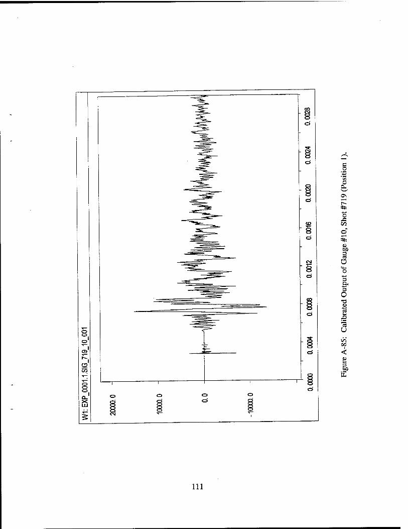
e .2
CO
O PM ^^ ON
r- *t= +■» o CO
Ü o *-> 3 & 3 o
jD
U
00
3
111
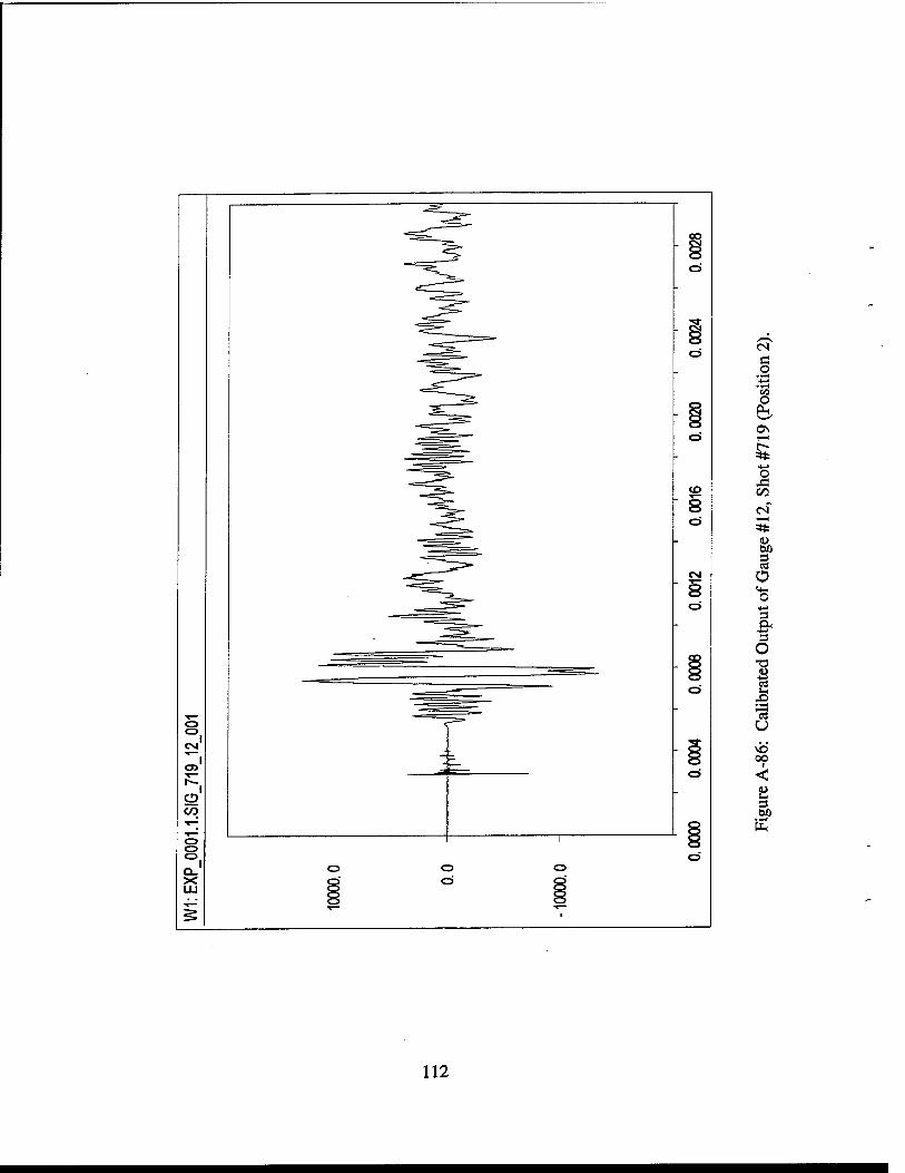
C o CO
O PL, ^^ ON T—I
o CO
of
50
O O
s & 3 o
I U so 00
2 3
112
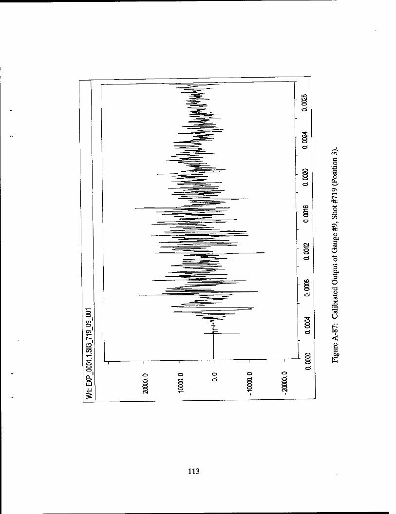
■S CO
x
. =
e o CO O
Oj,
Os
o co as
Ü (4-1 o 3 & 3 o
I 'S u 03
o Ö
113
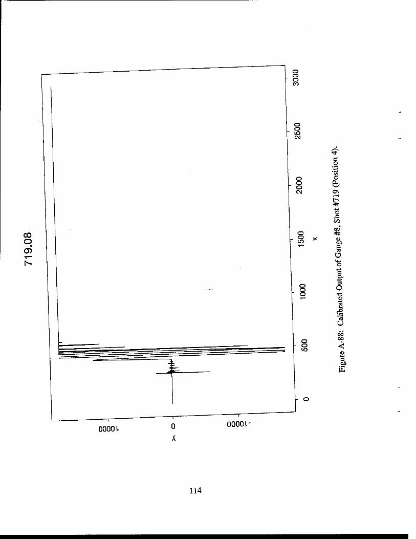
00 q 05
g • 1—I
O
ON T—I
o CO
00 m=
<u oß
Ü «4-1 o
& o
I U 00 00
8
tu
114
«n G O
o OH s_> ON 1-H t~- *t O
CO
Ü <4-H o
i- o
1 I U ON 00
8 3
E
115
G .2 O
OH,
ON T-l
■4->
O JA 00
SO
g Ü «4-1 o +■> 3 a- s- O <D
CO
U Ö
8
116
es
O
o\ t—I
o
<D
Ü o
3 o
I "ÖS u o\
2
117
oo
§
o
1—1
CO
=8= (SO u o
<4-l o
o
2
Ü
ON
3
118
ON
Ö
O OH ^—' ON *—i
& o
00
en
Ü o
I 3 O
2
U en ON
ß 3 00
119
g CO
O OH \s OS
*-> o
CO
CO
O o
■4-J
3 & S O
I "öS U
ON
2 3
IS
120
§
o
ON
o v5
DO
O o 3 & 3 o
1 U
>n
ß s
121
CO
O OH ^^ 0\ i—i
CO
(50
O 'S
s o
ON
8 (50
122
Appendix B
Normalized Data - Each Shot
123

This page intentionally left blank
124
o CD
O
o CM
O O
O CO
g) CO sz o E o © Ü c & to
o CO
o
o CM
ere 9"S 0"2 Q'L OH
epniiidujv pazjiBUJJON
ON VO
O
CO
c 'o
Ä CO
a
"8 .a 'S
O z
PQ
8 3>
125
o CD
O
o CM
CO
E»
2 o E p CD ü c 05
O w 00 Q
o CO
o
o CM
CO ON
o CO
g 'o OH
CO
I o
«1
Q >>
•8 B
T3
13
i PQ 8 s bo E
0"2 9" I OH
epnijidiuv peziiBouoN
126
O) (0
O E B o <«
* S O c
to
ere 9'2 0"2 S"t OH
9pn;i|dLUV paziieuwoN
Q'O
00 o
o CO
o ^1
■a CO
s
u
Q 3
CO
-8 3
U
O Z
PQ
I
127
o CD
ON
o O
4-* o Ä t/3
i
C 'o
o (X, CM ^ T—
8
CD o O) ,lH
o ca .c o Ü s E B o • i-H
Q CD >> Ü X>
o 00
c CO
"S3 h
«1
5
o CO
o
o CM
ere 9'Z VZ 9'i OH
apnyidiuv paziieuuoN
128
o-e 9-2 O'Z SH OH
epnwdujv pezpuuoN
9-0
129
o CO
o •<*•
CO 1—1
CO o 1 CM *J
e 'o OH
CD 8 CO Ä CO
CO O O Ü R
E ft o «
**— u CD 5 Ü 4>S c CO Q
O CO ^ CO a
o CO
o
o C\J
o-e 9'2 0'2 9H OH
spnjjidiuv P9Z!|BLUJO[S|
v© i
a 8
130
o CO
o •* ,
=8:
00
o ■u CM C
1 CD ja OJ C/3
fi u .c o l_J O Ä b o o o >_ **~ cd CD O c CO Q "K ;>■> o CO £ oo Q
3
o CD
O
* CM
OX S'Z O'Z 9" I OH
spniiidaiv PSZHBLUJON
« 8 S)
131
0\
5 o
00
•S o OH
4S
a) S p as .c Ü E p
CD Ü C
"55 CO t>
a
"8 "c3
66 PQ 8 D
E
ere S"Z 0"Z 9-1- CU
epninduiv pazpiwoN
132
NO. OF COPIES ORGANIZATION
2 DEFENSE TECHNICAL INFORMATION CENTER DTICDDA 8725 JOHN J KTNGMAN RD STE0944 FT BELVOIR VA 22060-6218
1 HQDA DAMOFDQ DENNIS SCHMIDT 400 ARMY PENTAGON WASHINGTON DC 20310-0460
1 CECOM SP & TRRSTRL COMMCTN DTV AMSEL RD ST MC M HSOICHER FT MONMOUTH NJ 07703-5203
1 PRINDPTYFORTCHNLGYHQ USARMYMATCOM AMCDCGT MFISETTE 5001 EISENHOWER AVE ALEXANDRIA VA 22333-0001
1 PRINDPTYFORACQUSTNHQS USARMYMATCOM AMCDCG A D ADAMS 5001 EISENHOWER AVE ALEXANDRIA VA 22333-0001
1 DPTY CG FOR RDE HQS USARMYMATCOM AMCRD BGBEAUCHAMP 5001 EISENHOWER AVE ALEXANDRIA VA 22333-0001
1 DPTY ASSIST SCY FOR R&T SARDTT TRILLION THE PENTAGON WASHINGTON DC 20310-0103
1 OSD OUSD(A&T)/ODDDR&E(R) JLUPO THE PENTAGON WASHINGTON DC 20301-7100
NO. OF COPIES ORGANIZATION
1 INSTFORADVNCDTCHNLGY THE UNIV OF TEXAS AT AUSTIN PO BOX 202797 AUSTIN TX 78720-2797
1 USAASA MOASAI WPARRON 9325 GUNSTON RD STE N319 FT BELVOIR VA 22060-5582
1 CECOM PMGPS COLS YOUNG FT MONMOUTH NJ 07703
1 GPS JOINT PROG OFC DIR COL J CLAY 2435 VELA WAY STE 1613 LOS ANGELES AFB CA 90245-5500
1 ELECTRONIC SYS DIV DIR CECOM RDEC JNJEMELA FT MONMOUTH NJ 07703
3 DARPA L STOTTS J PENNELLA B KASPAR 3701 N FAIRFAX DR ARLINGTON VA 22203-1714
1 SPCL ASST TO WING CMNDR 50SW/CCX CAPT P H BERNSTEIN 300 0"MALLEY AVE STE 20 FALCON AFB CO 80912-3020
1 USAF SMC/CED DMA/JPO MISON 2435 VELA WAY STE 1613 LOS ANGELES AFB CA 90245-5500
1 US MILITARY ACADEMY MATH SCI CTR OF EXCELLENCE DEPT OF MATHEMATICAL SCI MDN A MAJ DON ENGEN THAYERHALL WEST POINT NY 10996-1786
133
NO. OF COPIES ORGANIZATION
1 DIRECTOR US ARMY RESEARCH LAB AMSRLCSALTP 2800 POWDER MILL RD ADELPHI MD 20783-1145
1 DIRECTOR US ARMY RESEARCH LAB AMSRLCSALTA 2800 POWDER MILL RD ADELPHI MD 20783-1145
3 DIRECTOR US ARMY RESEARCH LAB AMSRLCILL 2800 POWDER MILL RD ADELPHI MD 20783-1145
ABERDEEN PROVING GROUND
4 DIRUSARL AMSRLCILP(305)
134
NO. OF COPIES ORGANIZATION
1 OSD OUSD AT STRTTACSYS DRSCHNETTER 3090 DEFNS PENTAGON RM 3E130 WASHINGTON DC 20301-3090
1 ASST SECY ARMY RESEARCH DEVELOPMENT ACQUISITION SARDZD RM2E673 103 ARMY PENTAGON WASHINGTON DC 20310-0103
1 ASST SECY ARMY RESEARCH DEVELOPMENT ACQUISITION SARDZP RM2E661 103 ARMY PENTAGON WASHINGTON DC 20310-0103
1 ASST SECY ARMY RESEARCH DEVELOPMENT ACQUISITION SARDZS RM3E448 103 ARMY PENTAGON WASHINGTON DC 20310-0103
1 ASST SECY ARMY RESEARCH DEVELOPMENT ACQUISITION SARD ZT RM 3E374 103 ARMY PENTAGON WASHINGTON DC 20310-0103
1 UNDER SEC OF THE ARMY DUSA OR RM2E660 102 ARMY PENTAGON WASHINGTON DC 20310-0102
1 ASST DEP CHIEF OF STAFF OPERATIONS AND PLANS DAMOFDZ RM3A522 460 ARMY PENTAGON WASHINGTON DC 20310-0460
1 DEPUTY CHIEF OF STAFF OPERATIONS AND PLANS DAMO SW RM 3C630 400 ARMY PENTAGON WASHINGTON DC 20310-0400
NO. OF COPIES ORGANIZATION
1 ARMY RESEARCH LABORATORY AMSRLSL PROGRAMS AND PLANS MGR WSMRNM 88002-5513
ABERDEEN PROVING GROUND
1 CDRUSATECOM AMSTE-TA
2 DIRUSAMSAA AMXSY-ST AMXSY-D
4 DIRUSARL AMSRL-SL, J WADE (433) M STARKS (433) AMSRL-SL-C, J BEILFUSS (E3331) AMSRL-SL-B, P DEITZ (328)
135
NO. OF COPIES ORGANIZATION
NO. OF COPIES ORGANIZATION
1 DIR OPERATIONAL TEST &EVAL ERNEST SEGLIE RM3E318 1700 DEFENSE PENTAGON WASHINGTON DC 20301-1700
1 DIR OPERATIONAL TEST &EVAL JAMES FO'BRYON RM 1C730A 1700 DEFENSE PENTAGON WASHINGTON DC 20301-1700
1 ODDRNEAT DIR WEAPONS TECH ATTN WES KITCHENS 3080 DEFENSE PENTAGON WASHINGTON DC 20301-3080
1 UNDER SECY OF THE ARMY SAUS OR DANIEL WDLLARD 102 ARMY PENTAGON WASHINGTON DC 20310-0102
1 ASST SECY ARMY RESEARCH DEVELOPMENT ACQUISITION SARD ZD DR HERBERT FALLIN RM 2E673 103 ARMY PENTAGON WASHINGTON DC 20310-0103
1 ASST SECY ARMY RESEARCH DEVELOPMENT ACQUISITION SARD TR TOM KULION RM3E480 103 ARMY PENTAGON WASHINGTON DC 20310-0103
1 USARASCXRA HUGHGRTFFIS BLDG16 2275DSTSUTTE10 WRIGHT PATTERSON AFB OH 45433-7227
1 USARLWLMNS LANNYGBURDGE 101 WEST EGLINBLVD SUITE 302 EGLIN AFB FL 32542-6810
4 ARMY RESEARCH OFFICE MATH AND CSDIV DRJCHANDRA KCLARK DRWU DR MING LING RESEARCH TRIANGLE PARK NC 27709-2211
1 DEFENSE NUCLEAR AGENCY WE MICHAEL GILTRUDE 6801 TELEGRAPH RD ALEXANDRIA VA 22310-3398
1 DEFENSE NUCLEAR AGENCY ATTNOFTA DR. MICHAEL SHORE 6801 TELEGRAPH RD ALEXANDRIA VA 22310-3398
1 DIRLLNL MILTON FINGER L159 PO BOX 808 LTVERMORECA 94551
NAVAL SURFACE WARFARE CTR DAHLGREN DIVISION GS4TOMWASMUND 17320 DAHLGREN RD DAHLGREN VA 22448-5100
DIRLLNL CONV WEAPON TCHNLGS JOSEPH REPA MS A133 PO BOX 1663 LOS ALAMOS NM 87545
USAMICOM AMSMIRD PAULLJACOBS REDSTONE ARSENAL AL 35898-5420
136
NO. OF COPIES ORGANIZATION
1 NWSCDL JTCG ME PRGRM OFC G202 GEORGE A WILLIAMS BLDG 221 RM 245 DAHLGREN VA 22448-5100
1 US MILITARY ACADEMY DEPTOFMATHSCI MAJDAVEOLWELL THAYERHALL WEST POINT NY 10996-1786
1 APPLIED RES ASSOC INC FRANK MAESTAS SUITE A220 4300 SAN MATEO BLVD ALBUQUERQUE NM 87110
1 APPLIED RES ASSOC INC RICH SCUNGIO 219 W BEL AVE SUITE 5 ABERDEEN MD 21001
ABERDEEN PROVING GROUND
1 CDROPTECEAC CSTEEAC BLDG 245 LDELATTRE
15 DIRUSARL ATTN: AMSRL-WM-PD,B.BURNS
AMSRL-WM-TD, D. DIETRICH AMSRL-WM-M, J. WALBERT AMSRL-IS-CI, B. BODT AMSRL-SL, P. TANENBAUM AMSRL-SL-BE,
D.BELY R. GROTE D. PETTY M. SIVACK J. T. KLOPCIC M.MAHAFFEY
AMSRL-SL-BG, A. YOUNG AMSRL-SL-BL,
M. RTTONDO J.HUNT
AMSRL-SL-BN, D. FARENWALD
137

LSfTENTIONAIJLY LEFT BLANK.
138

REPORT DOCUMENTATION PAGE Form Approved OMB No. 0704-0188
Public »porting burd«i tor this collodion of Information Is estimated to «rerage 1 hour per response, Including tfte am. lor '"^'"^»J^ """*"L^S^iSL'S'JSf gatherlngand maintaining the data nwM, and complying and reviewing th, collection of Information Send comnMntsragarolng thlsl*"£""^ " ^^3??£'j«on colleetlon of information, including suggostlons for reducing this burden, to Washington Headquarters Services, Kreetorate 'o^n'ormatlon^°ZZSZ5T,KS n^.Hiohw», suit.1^ »Hin^n vA nx,7+v» and to m. OHice of Mfm.tKm.Hii[und Bnrrnftt PMMimrr, ^""^ f?™?™, ff?'""""',""!"!' 1. AGENCY USE ONLY (Lam» Wan*; 2. REPORT DATE
November 1997
3. REPORT TYPE AND DATES COVERED
Final, Jul 95 - Jul 97 4. TITLE AND SUBTITLE
An Experiment, Analysis, and Model of Ballistic Shock
6. AUTHOR(S)
J. Terrence Klopcic, Walton T. Robinson, Donald W. Petty, and Michael R. Sivack
7. PERFORMING ORGANIZATION NAME(S) AND ADDRESS(ES)
U.S. Army Research Laboratory ATTN: AMSRL-SL-BS Aberdeen Proving Ground, MD 21005-5068
9. SPONSORING/MONITORING AGENCY NAMES(S) AND ADDRESS(ES)
5. FUNDING NUMBERS
AH80
8. PERFORMING ORGANIZATION REPORTNUMBER
ARL-MR-368
10.SPONSORING/MONITORING AGENCY REPORT NUMBER
11. SUPPLEMENTARY NOTES
12a. DISTRIBUTION/AVAILABILITY STATEMENT
Approved for public release; distribution is unlimited.
12b. DISTRIBUTION CODE
13. ABSTRACT (Maximum 200 words)
This study deals with the propagation of the leading, high-frequency edge of the shock wave emanating from an impact point on an armored vehicle, specifically, in an experiment on an Ml 13 armored personnel carrier subjected to explosive
charges.
The amplitude of the transverse wave can be well fit by a semiempirical equation, which accounts for both longitudinal and transverse waves, exponential decrease with distance, mixing of waves at edges, and amplification at points near edges. Comparison of wave speeds with published data confirms the roles of longitudinal and transverse disturbances.
14. SUBJECT TERMS
shock, ballistic shock, Ml 13
17. SECURITY CLASSIFICATION OF REPORT
UNCLASSIFIED
18. SECURITY CLASSIFICATION OF THIS PAGE
UNCLASSIFIED
19. SECURITY CLASSIFICATION OF ABSTRACT
UNCLASSIFIED
15. NUMBER OF PAGES
146 16. PRICE CODE
20. LIMITATION OF ABSTRACT
UL
NSN 7540-01-280-5500 139 Standard Form 298 (Rev. 2-89) Prescribed by ANSI Std. 239-18 298-102

INTENTIONALLY LEFT BLANK.
140

USER EVALUATION SHEET/CHANGE OF ADDRESS
This Laboratory undertakes a continuing effort to improve the quality of the reports it publishes. Your comments/answers to the items/questions below will aid us in our efforts.
1. ARL Report Number/Author ARL-MR-368 fKloPcic) Date of Report November 1997
2. Date Report Received
3. Does this report satisfy a need? (Comment on purpose, related projector other area of interest for which the report will
be used.) ——
4. Specifically, how is the report being used? (Information source, design data, procedure, source of ideas, etc.).
5. Has the information in this report led to any quantitative savings as far as man-hours or dollars saved, operating costs
avoided, or efficiencies achieved, etc? If so, please elaborate. _
6. General Comments. What do you think should be changed to improve future reports? (Indicate changes to organization,
technical content, format, etc.)
Organization
CURRENT Name E-mail Name ADDRESS .
Street or P.O. Box No.
City, State, Zip Code
7. If indicating a Change of Address or Address Correction, please provide the Current or Correct address above and the Old
or Incorrect address below.
Organization
OLD Name ADDRESS
Street or P.O. Box No.
City, State, Zip Code
(Remove this sheet, fold as indicated, tape closed, and mail.) (DO NOT STAPLE)
DEPARTMENT OF THE ARMY
OFFICIAL BUSINESS
BUSINESS REPLY MAIL FIRST CLASS PERMIT NO 0001,APG,MD
POSTAGE WILL BE PAID BY ADDRESSEE
DIRECTOR US ARMY RESEARCH LABORATORY ATTN AMSRLSLBS ABERDEEN PROVING GROUND MD 21005-5068
NO POSTAGE NECESSARY
IF MAILED IN THE
UNITED STATES