Embed Size (px)
Citation preview

An Extended Finite Element Method (XFEM) approach to hydraulic fractures:
Modelling of oriented perforations
Miguel Teixeira Luís Fialho Medinas
Thesis to obtain the Master of Science Degree in
Petroleum Engineering
Supervisor: Prof. Teresa Maria Bodas de Araújo Freitas
Examination Committee
Chairperson: Prof. Maria João Correia Colunas Pereira Supervisor: Prof. Teresa Maria Bodas de Araújo Freitas
Members of the Committee: Prof. Maria Matilde Mourão de Oliveira Carvalho Horta Costa e Silva
July 2015

Acknowledgements
To my mother and father for all the support given during my academic path. It was and is
essential for me to keep fighting for my unachievable objectives.
To my sisters for all the academic competition during all our life, which pushed me beyond my
limits and probably will still happen for the rest of our lives.
To Prof. Teresa Bodas Freitas for the support given in the execution of this study and document,
as well as all the kindness since the ECA’s course.
To Joana for all the late nights in McDonalds and for the essential support since the third year
at IST, remembering me that I was able to do not only two Master’s Degree at the same time
but also a post-graduation and all the other certifications.
To my MEP colleagues, Bruno Melo and João Brito during these last two years, for the shared
knowledge and academic experiences.

ii
Abstract
In the current context of energy markets global dynamics, production of Shale Reservoirs has
been a change in the energy paradigm, with the unconventional reservoirs now seen as a
potential "game changer".
The Hydraulic Fracturing (HF) technique is used to maximize their economic potential. Due to
the high cost of hydraulic fracturing operations, is essential to build reliable tools to predict the
formations behavior, and for this purpose, computer modeling of hydraulically induced fractures
is an important method to study fracture parameters, such as length, width or fracture efficiency
(fluid loss), amongst others.
In general, software used in the industry for fracture modelling allows very few independent
input parameters. In contrast, recent advances in available numerical methods – in particular
the extended finite element method (XFEM) – have increased the fracture modelling
capabilities. The XFEM (extended Finite Element Method), is a new method for
discontinuities/fractures modelling, based on the concept of local nodal enrichment functions
and phantom nodes, which reduces the convergence problems and increases the results
accuracy, and is used in the study presented herein.
To validate the numerical tools, numerical simulations of a series of laboratory tests that
reproduce hydraulic fracturing by oriented perforations on rectangular blocks of gypsum
cement by Abass H. et al. (1994) were carried out. The numerical results provide a good match
to the experimental observations.
Following that, a parametric study was carried out on the effect of a series of parameters on the
outcome of hydraulic fracturing operations, in terms of fracture initiation, propagation and
reorientation, when using 180°-phased oriented perforations.
It was found that various variables influence the fracture behavior; of those considered in this
study, flow rate, stress anisotropy, rock permeability and phasing were found to introduce major
changes in fracture initiation, propagation, reorientation and width.
Keywords: Hydraulic Fracturing, XFEM, oriented perforations, hydro-geomechanical model,
fracture propagation

iii
Resumo
No contexto das atuais dinâmicas globais do mercado da energia, a exploração e produção de
reservatórios de Argilitos laminados introduziu uma mudança no paradigma energético, sendo
os reservatórios não convencionais hoje vistos como um potencial “game changer”.
A fracturação hidráulica (FH) é utilizada para maximizar o seu potencial económico. No entanto,
dados os elevados custos destas operações, torna-se essencial a construção de ferramentas para
prever o comportamento das formações, e nesse sentido, a modelação numérica de fracturas
induzidas hidraulicamente é um método importante para estudar diversos parâmetros, como o
comprimento, abertura ou eficiência da fractura.
Em geral, os softwares utilizados na indústria para a modelação de fracturas permitem a
introdução de poucos parâmetros de entrada independentes. Por oposição, avanços recentes
em métodos numéricos disponíveis - em particular o Método dos Elementos Finitos
Alargado/Extendido (XFEM) - aumenta a capacidade de modelação de fracturas. O XFEM, é um
novo método para a modelação de descontinuidades/singularidades, baseado nos conceitos de
enriquecimento dos nós e nós-fantasma, que permitem reduzir problemas de convergência e
aumentar a precisão dos resultados, sendo usado no presente estudo.
Por forma a validar a ferramenta de cálculo, procedeu-se à simulação de uma série de ensaios
experimentais descritos por Abass et al. (1994), efetuados em laboratório sob provetes de gesso
consolidados em câmara de triaxial verdadeiro. Os resultados numéricos apresentam boa
concordância com os dados experimentais.
Em seguida, procedeu-se à execução de um estudo paramétrico sobre o efeito de um conjunto
de parâmetros nos resultados de uma operação de fracturação hidráulica, em termos da
iniciação, propagação e reorientação da fractura, considerando perfurações orientadas com fase
180°.
Verificou-se que diferentes variáveis influenciam o comportamento da fractura; das
consideradas, o caudal de injecção, anisotropia de tensões, permeabilidade e fase das
perfurações verificou-se introduzirem alterações significativas na iniciação, propagação,
reorientação e abertura da fractura.
Palavras-chave: Fracturação hidráulica, XFEM, perfurações orientadas, modelo hidro-
geomecânico, propagação da fractura.

iv
Contents
Acknowledgements ........................................................................................................................ i
Abstract ......................................................................................................................................... ii
Resumo ......................................................................................................................................... iii
I - Index de Figures ...................................................................................................................... viii
II - Tables ...................................................................................................................................... xii
III - Index of Symbols ................................................................................................................... xiii
IV - Index of Abbreviations .......................................................................................................... xvi
1. Introduction .......................................................................................................................... 1
1.1 Context ................................................................................................................................ 1
1.2 Objectives ............................................................................................................................ 2
1.3 Structure .............................................................................................................................. 3
Theoretical framework .......................................................................................................... 3
Modeling - Validation ............................................................................................................ 3
Modelling – Parametric study ............................................................................................... 4
Conclusions ........................................................................................................................... 4
2. Hydraulic Fracturing .............................................................................................................. 5
2.1 Introduction......................................................................................................................... 5
2.2 Technique History ............................................................................................................... 5
2.3 Hydraulic fracturing operation ............................................................................................ 6
2.4 Perforations ......................................................................................................................... 7
2.5 Numerical studies on hydraulic fracturing – state of the art ............................................. 8
3. Material Mechanics ............................................................................................................. 12
3.1 Introduction....................................................................................................................... 12
3.2 Rock Mechanics ................................................................................................................. 12
3.2.1 Constitutive laws ........................................................................................................ 12
Linear Elastic model ........................................................................................................ 12
Poroelasticity and the influence of pore pressure .......................................................... 13

v
3.2.2 Failure criteria ............................................................................................................ 14
Shear failure criteria ........................................................................................................ 14
Tensile failure criteria ...................................................................................................... 15
3.2.3 In-situ stresses ............................................................................................................ 15
Vertical stresses............................................................................................................... 15
Horizontal stresses .......................................................................................................... 15
Tectonic stress regimes ................................................................................................... 16
3.2.4 Stress changes near wellbore due to HF .................................................................... 17
3.3 Linear elastic fracture mechanics ...................................................................................... 19
3.3.1 Stress Distribution around the fracture tip ................................................................ 19
3.3.2 Crack Loading Modes ................................................................................................. 20
3.3.3 Stress Intensity factors ............................................................................................... 20
3.3.4 Griffith energy balance equation ............................................................................... 22
3.3.5 The energy release rate – G ....................................................................................... 24
3.3.6 Failure Criteria ............................................................................................................ 24
3.3.7 J-Integral ..................................................................................................................... 25
3.4 Fluid Mechanics ................................................................................................................. 26
3.4.1 Material behavior and constitutive equations ........................................................... 26
Basic concepts ................................................................................................................. 26
Rheological models ......................................................................................................... 26
3.4.2 Fluid Flow – Hydraulic transport in rocks ................................................................... 28
Darcy law ......................................................................................................................... 28
Flow regimes ................................................................................................................... 29
Forchheimer Equation and Non-Darcy Flow Correction ................................................. 30
3.4.3 Fluid flow within a Fracture........................................................................................ 31
4. Numerical methods for fracture analysis ............................................................................ 33
4.1 Introduction....................................................................................................................... 33
4.2 Finite Element Method (FEM) ........................................................................................... 33

vi
4.2.1 Virtual work theorem ................................................................................................. 34
4.2.2 Discretization of the elements ................................................................................... 36
4.3 Partition of the Unity ......................................................................................................... 37
4.3.1 Partition of Unity Finite Element Method .................................................................. 38
4.3.2 Generalized Finite element method .......................................................................... 38
4.4 Extended Finite Element Method (XFEM) ......................................................................... 39
4.4.1 Enrichment functions ................................................................................................. 41
Heaviside/jump functions ............................................................................................... 42
Near-tip asymptotic functions......................................................................................... 42
4.4.2 Level Set Method ....................................................................................................... 43
4.4.3 Fracture propagation criteria ..................................................................................... 45
4.4.4 XFEM limitations ........................................................................................................ 46
5. Modelling ............................................................................................................................ 48
5.1 Introduction....................................................................................................................... 48
5.2 Numerical modelling of the fracture toughness determination test ................................ 48
5.2.1 Fracture Toughness determination ............................................................................ 48
5.2.2 Model initialization/Pre-processing ........................................................................... 49
5.2.3 Results and discussion ................................................................................................ 52
5.3 Numerical modelling of oriented perforations ................................................................. 53
5.3.1 Experimental setup and material parameters ........................................................... 54
5.3.2 Material parameters .................................................................................................. 56
5.3.3 Model geometry and finite element mesh ................................................................ 58
5.3.4 Boundary condition and loading procedure .............................................................. 60
5.3.4 Results and discussion ................................................................................................ 62
Geostatic – Near-wellbore stresses equilibrium ............................................................. 62
Breakdown pressure without perforation ...................................................................... 64
Breakdown pressure with oriented perforations............................................................ 65
Fracture reorientation ..................................................................................................... 67

vii
Fracture Width ................................................................................................................ 72
Fracture Pressure profile ................................................................................................. 74
6. Validation - Parametric study .............................................................................................. 76
6.1 Porosity ............................................................................................................................. 76
6.2 Permeability ...................................................................................................................... 76
6.3 Friction coefficient ............................................................................................................ 79
6.4 Stress Anisotropy .............................................................................................................. 80
6.5 Fluid viscosity .................................................................................................................... 84
6.6 Fluid leak-off ...................................................................................................................... 86
6.7 Flow rates .......................................................................................................................... 87
6.8 Different phasing ............................................................................................................... 90
6.9 Phasing misalignment ....................................................................................................... 92
7. Conclusions and future work .............................................................................................. 94
References ................................................................................................................................... 98
Annex - A.1 Execution of an Abaqus© XFEM analysis .................................................................. a
A 1.1 Abaqus Software structure .............................................................................................. a
A1.2 Components of the Abaqus Pre-processing phase ........................................................... b
Geometry and Material properties ................................................................................... b
Loads and Boundary Conditions .........................................................................................c
Output Data ........................................................................................................................c
A1.3 Abaqus/CAE modules .........................................................................................................c
viii
I - Index de Figures
Figure 2.1 - A typical two-phases fracturing chart with discretization of time steps (Daneshy A.,
2010) ............................................................................................................................................. 7
Figure 2.2 - Perforations phasing designs (Petrowiki, 2015) ........................................................ 8
Figure 3.1 - Principal stresses in normal faulting (NN) (left), strike-slip (SS) (middle) and reverse
faulting(RF) (right) regimes (Zoback M., 2007) ........................................................................... 16
Figure 3.2 - Crack behavior in the near tip region (Abass H. et Neda J., 1988); ......................... 19
Figure 3.3 - Barenblatt theory for crack tip (Charlez A. Ph., 1997) ............................................. 19
Figure 3.4 - Crack loading modes (Fjaer, 2008) ........................................................................... 20
Figure 3.5 - Schematic representation of crack tip stresses defined in polar coordinates ......... 21
Figure 3.6 - Griffith energy balance for an elliptical shape crack ................................................ 23
Figure 3.7 - Schematic representation of the 2D line J-Integral (Dassault Systémes, 2015) ...... 25
Figure 3.8 - Fluid types based on the rheological curves (Valkó P. et Economides M. J., 1995) 27
Figure 3.9 - Flow zones in porous media. Flow through porous media can be classified into three
different flow zones, depending on local fluid velocity within the pore space (Basak P., 1977) 29
Figure 3.10 - 2D schematic Hydraulic fracture representation (Adachi, J. et al, 2007) .............. 31
Figure 4.1 - FEM domain for application of virtual work principle (adapted from (Mohammadi S.,
2008)) .......................................................................................................................................... 34
Figure 4.2 - Mapping of a Finite element in global and local coordinates (Mohammadi S., 2008)
..................................................................................................................................................... 35
Figure 4.3 - Finite elements discretization for 2D and 3D classical fracture mechanics (
(Mohammadi S., 2008) ................................................................................................................ 36
Figure 4.4 - Construction of the spider-web mesh, based on the degeneration of quadrilateral
elements in triangular elements (Dassault Systémes, 2013) ...................................................... 37
Figure 4.5 - Partition of unity concept (Wikipedia, 2015) - Ni, i = ηi ......................................... 37
Figure 4.6 - Definition of the enriched nodes in a mesh of finite elements (Duarte A. et Simone
A., 2012) ...................................................................................................................................... 39
Figure 4.7 - Enriched nodes by the discontinuity contour line in the interior or on the edge of the
element (Duarte A. et Simone A., 2012) ..................................................................................... 40
Figure 4.8 - Definition of the enriched nodes and domains in XFEM : Light grey – Heaviside
function ; Heavy grey – Near-tip functions ((Thoi T. N. et al, 2015) and (Natarajan S. et al, 2011))
..................................................................................................................................................... 41
Figure 4.9 - Strong and weak discontinuity definition, adapted from (Chaves E. W. et Oliver J.,
2001) and (Ayala G., 2006) .......................................................................................................... 41

ix
Figure 4.10 - Heaviside function (a)) and schematic representation of it in a finite element (b))
((Mohammadi S., 2008) and (Ahmed A., 2009)). ....................................................................... 42
Figure 4.11 - Near-tip enrichment functions (Ahmed A., 2009) ................................................. 43
Figure 4.12 - Enrichment function (b) modelling the crack in a partially cut tip element (Ahmed
A., 2009) ...................................................................................................................................... 43
Figure 4.13 - Level set functions representation (Zhen-zhong D, 2009) ..................................... 44
Figure 4.14 - Normal LSF for an interior crack (Gigliotti L., 2012) ............................................... 45
Figure 4.15 - Tangential LSF for an interior crack (Gigliotti L., 2012) .......................................... 45
Figure 4.16 - Schematic representation of the Abaqus© enrichment functions for stationary and
propagating singularities (Oliveira F., 2013) ............................................................................... 47
Figure 5.1 - Set up for fracture toughness determination - infinite plate with known central crack
under tension (Economides M. J. et al, 2000) ............................................................................. 49
Figure 5.2 - Geometry, boundary conditions and loads for fracture toughness test ................. 50
Figure 5.3 - Linear quadrilateral element degeneration (Dassault Systémes, 2015) .................. 51
Figure 5.4 - Mesh degeneracy to r=1/4 (Dassault Systémes, 2015)............................................ 51
Figure 5.5 - Mesh around the crack tip/singularity ..................................................................... 51
Figure 5.6 - Mesh geometry for the propagation XFEM and contour integral stationary crack . 52
Figure 5.7 - Crack propagation initiation based on XFEM model ................................................ 52
Figure 5.8 - Contour stress intensity factors for F=288KN .......................................................... 53
Figure 5.9 - Core sample geometry, wellbore and perforations (Abass H. et al, 1994) .............. 54
Figure 5.10-Perforations direction relative to the PFP b) ........................................................... 54
Figure 5.11 - Schematic of a true-triaxial hydraulic fracturing test system (Chen M. et al, 2010)
..................................................................................................................................................... 55
Figure 5.12 - Interior design of a true-triaxial apparatus (Frash L. P. et al, 2014) ...................... 55
Figure 5.13 - Energy-based damage evolution for linear softening (Dassault Systémes, 2015) . 57
Figure 5.14 - Model geometry and partition faces ..................................................................... 58
Figure 5.15 - Different Mesh configuration for XFEM oriented perforations study ................... 59
Figure 5.16 - Displacement boundary conditions for the oriented perforations experience ..... 60
Figure 5.17 - Fluid Injection amplitude through time ................................................................. 61
Figure 5.18- Typical fracture pressure profile during and post-injection (Soliman M. Y. et Boonen
P., 2000) ...................................................................................................................................... 61
Figure 5.19 - Stress initialization due to wellbore excavation .................................................... 63
Figure 5.20 - Pore pressure distribution in the sample with the start of fluid injection ............ 64
Figure 5.21 - Breakdown pressure comparison between (Abass, 1994) and the numerical
simulation .................................................................................................................................... 66
x
Figure 5.22 - Tangential stresses in the initial geostatic equilibrium and through the tensile
failure in the crack tip ................................................................................................................. 66
Figure 5.23 - Tangential stresses in crack tip for numerical and laboratorial results ................. 67
Figure 5.24 - Comparison of model simulation results with experimental results ..................... 68
Figure 5.25 - Fracture reorientation for all perforation directions ............................................. 69
Figure 5.26 - Schematic representation of reorientation radius (Chen M. et al, 2010).............. 70
Figure 5.27 - Stress Anisotropy ratios for different moments in the crack propagation for 90°
perforation angle ........................................................................................................................ 71
Figure 5.28 - Fracture propagation with fluid injection .............................................................. 73
Figure 5.29 - Fracture Pressure profile for perforation near-crack tip for direction 0 ............... 74
Figure 6.1 - Breakdown pressure for different directions and different permeabilities ............ 77
Figure 6.2 - Evolution of the injected flow with permeability for different perforation directions
..................................................................................................................................................... 77
Figure 6.3 - Fracture propagation for different permeabilities to a perforation in direction 45 78
Figure 6.4 - Fracture propagation for different permeabilities to a perforation in direction 90 78
Figure 6.5 - Injected flow for the complete reorientation to the PFP of 90° perforations ......... 79
Figure 6.6 - Fracture reorientation for different friction coefficients: a) 0,000001 ; b)0,0001 ; c)
0,001 ; d) 0,1 to a perforation 45° ............................................................................................... 80
Figure 6.7 - Injected flow to cause the rock tensile failure for different directions and anisotropy
ratios ........................................................................................................................................... 81
Figure 6.8 - Fracture propagation for different stress ratio in direction 90° .............................. 82
Figure 6.9 - Fracture propagation for different stress ratio in direction 45° .............................. 82
Figure 6.10 - Fracture reorientation for 45 and 90 perforations with a stress anisotropy ratio = 1
..................................................................................................................................................... 83
Figure 6.11 - Fracture reorientation for a 45° perforation with a stress anisotropy ratio = 0,5…83
Figure 6.12 - Parametric diagram representing the four limiting propagation regimes of
hydraulically induced fractures (Zielonka M. G. et al, 2014) ...................................................... 84
Figure 6.13 - Fracture reorientation for a direction 90° perforation for different viscosity. ...... 85
Figure 6.14 - Fluid leak-off coefficients (cT and cB) to the fracture computation, where
vT and vB are the top and bottom fluid displacement velocities and pf, pB, and pT are the
fracture, bottom and top pressures respectively (Zielonka M. G. et al, 2014) ........................... 86
Figure 6.15 - Fracture width by leak-off coefficients to a direction 0° perforation for an injected
flow = 2,5 × 10⁻⁶ m3 .................................................................................................................. 87
Figure 6.16 - Total injected fluid to cause for fracture initiation ................................................ 88

xi
Figure 6.17 - Fracture reorientation for perforation direction 45° and 90° to different injection
rates (m3/s) ................................................................................................................................. 89
Figure 6.18 - Fracture propagation distance vs. time for a direction 0° perforation ................. 89
Figure 6.19 - Fracture propagation for different perforation phasing ........................................ 91
Figure 6.20 - Fracture propagation for different phasing with perforation miss alignment ...... 92
Figure A.0.1 - Scheme of the interactive processing stages (Author) ........................................... a
Figure A.0.2 – Stress (left) and strain (right) controlled stress-strain curves (Hudson J. A. et
Harrisson J. P., 1997) ......................................................................................................................c
Figure A.0.3 - Abaqus/CAE interface ............................................................................................. d
Figure A.0.4 - Energy-based damage evolution for linear softening (Dassault Systémes, 2015) . e
Figure A.0.5 - Phantom nodes due to pore pressure extra degrees of freedom (original nodes are
represented with full circles and corner phantom nodes with hollow circles) (Zielonka M. G. et
al, 2014) ......................................................................................................................................... g
Figure A.0.6- Displacement boundary conditions for the XFEM modelling (Zielonka M. G. et al,
2014) ............................................................................................................................................. g
Figure A.0.7 - Concentrated flow injection in the phantom nodes/edge (Zielonka M. G. et al,
2014) ............................................................................................................................................. g
Figure A.0.8 - Quadrilateral element types (Forum 8, 2015) ........................................................ h
Figure A.0.9- Centroid vs Crack tip fracture propagation determination (Dassault Systémes,
2013) .............................................................................................................................................. i
xii
II - Tables
Table 3.1 - Reynolds number values associated with the different flow regimes (Amao A. M.,
2007) ........................................................................................................................................... 30
Table 4.1 - Differences between VCCT method and CZM - adapted from (Dassault Systémes,
2015) ........................................................................................................................................... 46
Table 5.1 - Input parameters for fracture toughness determination test .................................. 50
Table 5.2 - Physical and mechanical properties of Abass H. et al. (1994) samples..................... 56
Table 5.3 - 2D different mesh properties for XFEM oriented perforations study ...................... 59
Table 5.4 - Comparison between measured initial tangential stresses between analytical and
numerical solutions ..................................................................................................................... 63
Table 5.5 - Breakdown pressure for direction 0-90° for studied model ..................................... 65
Table 5.6 - Reorientation radius for different perforation angle ................................................ 70
Table 5.7 - Stress Anisotropy ratios for different moments in the crack propagation (at the
element level) for 90° perforation angle..................................................................................... 71
Table 5.8 - Fracture opening (mm) for different perforation direction to different injected flows
..................................................................................................................................................... 72
Table 5.9 - Fracture opening rate (Width function) verification to direction 90° ....................... 73
Table 5.10 - Equilibrium fracture pressure for different perforation direction after reorientation
to the PFP .................................................................................................................................... 74
Table 6.1 - Stress anisotropies .................................................................................................... 80
Table 6.2 - Breakdown pressure for different stress ration for perforation directions 0°, 45° and
90° ............................................................................................................................................... 80
Table 6.3 - Analytical breakdown pressure values for different stress ratios to direction 0° and
90° (without perforation) – Based on equation 3.12 .................................................................. 81
Table 6.4 – Breakdown pressure for different leak-off coefficients for perforation direction 0°.
..................................................................................................................................................... 86
Table 6.5 - Breakdown pressure by flow rate ............................................................................. 87
Table 6.6 - First and second breakdown pressure (MPa) for different phasing ......................... 91
Table 6.7 - First and second breakdown pressure (MPa) for different phasing ......................... 93

xiii
III - Index of Symbols
𝑁𝑖(𝑥)̅̅ ̅̅ ̅̅ ̅ − 𝑁𝑒𝑤 𝑠𝑒𝑡 𝑜𝑓 𝑠ℎ𝑎𝑝𝑒 𝑓𝑢𝑛𝑐𝑡𝑖𝑜𝑛𝑠
𝜎′00 − 𝐸𝑓𝑓𝑒𝑐𝑡𝑖𝑣𝑒 𝑡𝑎𝑛𝑔𝑒𝑛𝑡𝑖𝑎𝑙 𝑠𝑡𝑟𝑒𝑠𝑠
𝜎′𝑒𝑓𝑓𝑒𝑐𝑡𝑖𝑣𝑒 − 𝐸𝑓𝑓𝑒𝑐𝑡𝑖𝑣𝑒 𝑠𝑡𝑟𝑒𝑠𝑠𝑒𝑠
Π0 − 𝐼𝑛𝑖𝑡𝑖𝑎𝑙 𝑒𝑙𝑎𝑠𝑡𝑖𝑐 𝑝𝑜𝑡𝑒𝑛𝑡𝑖𝑎𝑙 𝑒𝑛𝑒𝑟𝑔𝑦
Ω𝑒 − 𝐸𝑙𝑒𝑚𝑒𝑛𝑡 𝑣𝑜𝑙𝑢𝑚𝑒
𝐴𝑐𝑜𝑚 − 𝐶𝑜𝑚𝑚𝑢𝑛𝑖𝑐𝑎𝑡𝑖𝑜𝑛 𝑎𝑟𝑒𝑎 𝑏𝑒𝑡𝑤𝑒𝑒𝑛 𝑡ℎ𝑒 𝑓𝑟𝑎𝑐𝑡𝑢𝑟𝑒 𝑎𝑛𝑑 𝑡ℎ𝑒 𝑝𝑒𝑟𝑓𝑜𝑟𝑎𝑡𝑖𝑜𝑛 𝑡𝑢𝑛𝑛𝑒𝑙
𝐴𝑚 − 𝐴𝑚𝑝𝑙𝑖𝑡𝑢𝑑𝑒 𝑑𝑖𝑚𝑒𝑛𝑠𝑖𝑜𝑛𝑙𝑒𝑠𝑠 𝑓𝑢𝑛𝑐𝑡𝑖𝑜𝑛 𝑑𝑒𝑝𝑒𝑛𝑑𝑒𝑛𝑡 𝑜𝑛 𝜃
𝐴𝑝𝑒𝑟𝑓 − 𝑃𝑒𝑟𝑓𝑜𝑟𝑎𝑡𝑖𝑜𝑛 𝑐𝑟𝑜𝑠𝑠 − 𝑠𝑒𝑐𝑡𝑖𝑜𝑛𝑎𝑙 𝑎𝑟𝑒𝑎
𝐵𝑖 − 𝐺𝑙𝑜𝑏𝑎𝑙 𝑚𝑎𝑡𝑟𝑖𝑥 𝑜𝑓 𝑑𝑖𝑠𝑝𝑙𝑎𝑐𝑒𝑚𝑒𝑛𝑡 − 𝑠𝑡𝑟𝑎𝑖𝑛
𝐶𝑓 − 𝐹𝑟𝑖𝑐𝑡𝑖𝑜𝑛 𝑐𝑜𝑒𝑓𝑓𝑖𝑐𝑖𝑒𝑛𝑡
𝐶𝑖𝑗𝑙𝑚 − 𝐶𝑜𝑛𝑠𝑡𝑖𝑡𝑢𝑡𝑖𝑣𝑒 𝑡𝑒𝑛𝑠𝑜𝑟
𝐶𝑙𝑒𝑎𝑘−𝑜𝑓𝑓 − 𝐿𝑒𝑎𝑘 − 𝑜𝑓𝑓 𝑐𝑜𝑒𝑓𝑓𝑖𝑐𝑖𝑒𝑛𝑡
𝐷(𝑒) − 𝑀𝑎𝑡𝑒𝑟𝑖𝑎𝑙 𝑠𝑡𝑟𝑒𝑠𝑠 − 𝑠𝑡𝑟𝑎𝑖𝑛 𝑚𝑎𝑡𝑟𝑖𝑥 − 𝑐𝑜𝑛𝑠𝑡𝑖𝑡𝑢𝑡𝑖𝑣𝑒 𝑚𝑎𝑡𝑟𝑖𝑥
𝐹𝑐 − 𝐶𝑟𝑖𝑡𝑖𝑐𝑎𝑙 𝑙𝑜𝑎𝑑
𝐺𝐼 − 𝐸𝑛𝑒𝑟𝑔𝑦 𝑟𝑒𝑙𝑒𝑎𝑠𝑒 𝑟𝑎𝑡𝑒 𝑓𝑜𝑟 𝑙𝑜𝑎𝑑𝑖𝑛𝑔 𝑚𝑜𝑑𝑒 𝐼
𝐺𝐼𝐶 − 𝐶𝑟𝑖𝑡𝑖𝑐𝑎𝑙 𝑒𝑛𝑒𝑟𝑔𝑦 𝑟𝑒𝑙𝑒𝑎𝑠𝑒 𝑟𝑎𝑡𝑒
𝐺𝐼𝐼 − 𝐸𝑛𝑒𝑟𝑔𝑦 𝑟𝑒𝑙𝑒𝑎𝑠𝑒 𝑟𝑎𝑡𝑒 𝑓𝑜𝑟 𝑙𝑜𝑎𝑑𝑖𝑛𝑔 𝑚𝑜𝑑𝑒 𝐼𝐼
𝐺𝐼𝐼𝐼 − 𝐸𝑛𝑒𝑟𝑔𝑦 𝑟𝑒𝑙𝑒𝑎𝑠𝑒 𝑟𝑎𝑡𝑒 𝑓𝑜𝑟 𝑙𝑜𝑎𝑑𝑖𝑛𝑔 𝑚𝑜𝑑𝑒 𝐼𝐼𝐼
𝐺𝑓 − 𝐹𝑟𝑎𝑐𝑡𝑢𝑟𝑒 𝑒𝑛𝑒𝑟𝑔𝑦
𝐽(𝑒) − 𝐸𝑙𝑒𝑚𝑒𝑛𝑡 𝑗𝑎𝑐𝑜𝑏𝑖𝑎𝑛 𝑚𝑎𝑡𝑟𝑖𝑥
𝐾𝐷 − 𝑆𝑒𝑡 𝑜𝑓 𝑒𝑛𝑟𝑖𝑐ℎ𝑒𝑑 𝑛𝑜𝑑𝑒𝑠 𝑎𝑠𝑠𝑜𝑐𝑖𝑎𝑡𝑒𝑑 𝑤𝑖𝑡ℎ 𝑑𝑖𝑠𝑐𝑜𝑛𝑡𝑖𝑛𝑢𝑖𝑡𝑖𝑒𝑠
𝐾𝐼 − 𝐹𝑟𝑎𝑐𝑡𝑢𝑟𝑒 𝑡𝑜𝑢𝑔ℎ𝑛𝑒𝑠𝑠 𝑓𝑜𝑟 𝑙𝑜𝑎𝑑𝑖𝑛𝑔 𝑚𝑜𝑑𝑒 𝐼
𝐾𝐼𝐶 − 𝐶𝑟𝑖𝑡𝑖𝑐𝑎𝑙 𝑓𝑟𝑎𝑐𝑡𝑢𝑟𝑒 𝑡𝑜𝑢𝑔ℎ𝑛𝑒𝑠𝑠
𝐾𝐼𝐼 − 𝐹𝑟𝑎𝑐𝑡𝑢𝑟𝑒 𝑡𝑜𝑢𝑔ℎ𝑛𝑒𝑠𝑠 𝑓𝑜𝑟 𝑙𝑜𝑎𝑑𝑖𝑛𝑔 𝑚𝑜𝑑𝑒 𝐼𝐼
𝐾𝐼𝐼𝐼 − 𝐹𝑟𝑎𝑐𝑡𝑢𝑟𝑒 𝑡𝑜𝑢𝑔ℎ𝑛𝑒𝑠𝑠 𝑓𝑜𝑟 𝑙𝑜𝑎𝑑𝑖𝑛𝑔 𝑚𝑜𝑑𝑒 𝐼𝐼𝐼
𝐾𝑇 − 𝑆𝑒𝑡 𝑜𝑓 𝑒𝑛𝑟𝑖𝑐ℎ𝑒𝑑 𝑛𝑜𝑑𝑒𝑠 𝑎𝑠𝑠𝑜𝑐𝑖𝑎𝑡𝑒𝑑 𝑤𝑖𝑡ℎ 𝑡ℎ𝑒 𝑐𝑟𝑎𝑐𝑘 𝑡𝑖𝑝
𝐾𝑒 − 𝐸𝑙𝑒𝑚𝑒𝑛𝑡 𝑠𝑡𝑖𝑓𝑛𝑒𝑠𝑠 𝑚𝑎𝑡𝑟𝑖𝑥
𝑁𝑖 − 𝑆ℎ𝑎𝑝𝑒 𝑓𝑢𝑛𝑐𝑡𝑖𝑜𝑛
𝑃𝐵𝐾 − 𝐵𝑟𝑒𝑎𝑘𝑑𝑜𝑤𝑛 𝑝𝑟𝑒𝑠𝑠𝑢𝑟𝑒
𝑃𝑓 − 𝐹𝑟𝑎𝑐𝑡𝑢𝑟𝑒 𝑝𝑟𝑒𝑠𝑠𝑢𝑟𝑒

xiv
𝑃𝑝 − 𝑃𝑜𝑟𝑒 𝑝𝑟𝑒𝑠𝑠𝑢𝑟𝑒
𝑄0 − 𝐹𝑙𝑢𝑖𝑑 𝑖𝑛𝑗𝑒𝑐𝑡𝑒𝑑 𝑖𝑛 𝑡ℎ𝑒 𝑓𝑟𝑎𝑐𝑡𝑢𝑟𝑒
𝑊𝑠 − 𝑊𝑜𝑟𝑘 𝑟𝑒𝑞𝑢𝑖𝑟𝑒𝑑 𝑡𝑜 𝑓𝑜𝑟𝑚 𝑡ℎ𝑒 𝑐𝑟𝑎𝑐𝑘
𝑎𝑖𝑗 − 𝐴𝑑𝑑𝑖𝑡𝑖𝑜𝑛𝑎𝑙 𝑑𝑒𝑔𝑟𝑒𝑒𝑠 𝑜𝑓 𝑓𝑟𝑒𝑒𝑑𝑜𝑚
𝑓𝑖𝑗 − 𝐷𝑖𝑚𝑒𝑛𝑠𝑖𝑜𝑛𝑙𝑒𝑠𝑠 𝑓𝑢𝑛𝑐𝑡𝑖𝑜𝑛 𝑑𝑒𝑝𝑒𝑛𝑑𝑒𝑛𝑡 𝑜𝑛 𝜃
𝑝𝑗(𝑥) − 𝐸𝑛𝑟𝑖𝑐ℎ𝑚𝑒𝑛𝑡 𝑓𝑢𝑛𝑐𝑡𝑖𝑜𝑛
𝑟𝑤 − 𝑊𝑒𝑙𝑙𝑏𝑜𝑟𝑒 𝑟𝑎𝑑𝑖𝑢𝑠
𝑢𝐸𝑛𝑟𝑖𝑐ℎ𝑚𝑒𝑛𝑡 − 𝐹𝑖𝑛𝑖𝑡𝑒 𝑒𝑙𝑒𝑚𝑒𝑛𝑡 𝑑𝑖𝑠𝑝𝑙𝑎𝑐𝑒𝑚𝑒𝑛𝑡 𝑑𝑢𝑒 𝑡𝑜 𝑒𝑛𝑟𝑖𝑐ℎ𝑒𝑑 𝑓𝑒𝑎𝑡𝑢𝑟𝑒𝑠
𝑢𝐹𝐸𝑀 − 𝑇𝑟𝑎𝑑𝑖𝑡𝑖𝑜𝑛𝑎𝑙 𝑓𝑖𝑛𝑖𝑡𝑒 𝑒𝑙𝑒𝑚𝑒𝑛𝑡 𝑑𝑖𝑠𝑝𝑙𝑎𝑐𝑒𝑚𝑒𝑛𝑡
𝑢𝑓 − 𝑇𝑜𝑡𝑎𝑙 𝑑𝑎𝑚𝑎𝑔𝑒 𝑓𝑟𝑎𝑐𝑡𝑢𝑟𝑒 𝑑𝑖𝑠𝑝𝑙𝑎𝑐𝑒𝑚𝑒𝑛𝑡
𝑢𝑥 − 𝐷𝑖𝑠𝑝𝑙𝑎𝑐𝑒𝑚𝑒𝑛𝑡 𝑖𝑛 𝑑𝑖𝑟𝑒𝑐𝑡𝑖𝑜𝑛 𝑥𝑥
𝑢𝑦 − 𝐷𝑖𝑠𝑝𝑙𝑎𝑐𝑒𝑚𝑒𝑛𝑡 𝑖𝑛 𝑑𝑖𝑟𝑒𝑐𝑡𝑖𝑜𝑛 𝑦𝑦
𝑤𝑓 − 𝐹𝑟𝑎𝑐𝑡𝑢𝑟𝑒 𝑤𝑖𝑑𝑡ℎ
𝛾𝑃 − 𝑃𝑙𝑎𝑠𝑡𝑖𝑐 𝑒𝑛𝑒𝑟𝑔𝑦 𝑜𝑓 𝑡ℎ𝑒 𝑚𝑎𝑡𝑒𝑟𝑖𝑎𝑙
𝛾𝑆 − 𝑆𝑢𝑟𝑓𝑎𝑐𝑒 𝑚𝑎𝑡𝑒𝑟𝑖𝑎𝑙 𝑒𝑛𝑒𝑟𝑔𝑦
휀𝑖𝑗 − 𝑆𝑡𝑟𝑎𝑖𝑛 𝑡𝑒𝑛𝑠𝑜𝑟
𝜂𝑖 − 𝐶𝑜𝑛𝑠𝑡𝑎𝑛𝑡 𝑠ℎ𝑎𝑝𝑒 𝑓𝑢𝑛𝑐𝑡𝑖𝑜𝑛
𝜌𝑤 − 𝑊𝑎𝑡𝑒𝑟 𝑑𝑒𝑛𝑠𝑖𝑡𝑦
𝜎ℎ − 𝑀𝑖𝑛𝑖𝑚𝑢𝑚 ℎ𝑜𝑟𝑖𝑧𝑜𝑛𝑡𝑎𝑙 𝑠𝑡𝑟𝑒𝑠𝑠
𝜎𝐻 − 𝑀𝑎𝑥𝑖𝑚𝑢𝑚 ℎ𝑜𝑟𝑖𝑧𝑜𝑛𝑡𝑎𝑙 𝑠𝑡𝑟𝑒𝑠𝑠
𝜎𝑇 − 𝑇𝑒𝑛𝑠𝑖𝑙𝑒 𝑠𝑡𝑟𝑒𝑛𝑔ℎ
𝜎𝑐 − 𝐶𝑜𝑚𝑝𝑟𝑒𝑠𝑠𝑖𝑣𝑒 𝑠𝑡𝑟𝑒𝑛𝑔ℎ
𝜎𝑓 − 𝐹𝑟𝑎𝑐𝑡𝑢𝑟𝑒 𝑠𝑡𝑟𝑒𝑠𝑠
𝜎𝑖𝑗 − 𝑆𝑡𝑟𝑒𝑠𝑠 𝑡𝑒𝑛𝑠𝑜𝑟
𝜎𝑟𝑟 = 𝑅𝑎𝑑𝑖𝑎𝑙 𝑠𝑡𝑟𝑒𝑠𝑠 𝑎𝑟𝑜𝑢𝑛𝑑 𝑡ℎ𝑒 𝑤𝑒𝑙𝑙𝑏𝑜𝑟𝑒
𝜎𝑦𝑜 = 𝜎𝑇
𝜎𝜃𝜃 − 𝑇𝑎𝑛𝑔𝑒𝑛𝑡𝑖𝑎𝑙 𝑠𝑡𝑟𝑒𝑠𝑠 𝑎𝑟𝑜𝑢𝑛𝑑 𝑡ℎ𝑒 𝑤𝑒𝑙𝑙𝑏𝑜𝑟𝑒
𝜕𝑖𝑗 − 𝐷𝑒𝑙𝑡𝑎 𝑑𝑖𝑟𝑎𝑐
2𝐵 − 𝐹𝑟𝑎𝑐𝑡𝑢𝑟𝑒 𝑡𝑜𝑢𝑔ℎ𝑛𝑒𝑠𝑠 𝑑𝑒𝑡𝑒𝑟𝑚𝑖𝑛𝑎𝑡𝑖𝑜𝑛 𝑠𝑎𝑚𝑝𝑙𝑒 𝑤𝑖𝑑𝑡ℎ
2𝐿 − 𝐹𝑟𝑎𝑐𝑡𝑢𝑟𝑒 𝑡𝑜𝑢𝑔ℎ𝑛𝑒𝑠𝑠 𝑑𝑒𝑡𝑒𝑟𝑚𝑖𝑛𝑎𝑡𝑖𝑜𝑛 𝑐𝑟𝑎𝑐𝑘 𝑙𝑒𝑛𝑔𝑡ℎ
Γ − 𝑂𝑢𝑡𝑤𝑎𝑟𝑑 𝑛𝑜𝑟𝑚𝑎𝑙

xv
Δ𝜎′00 − 𝑇𝑎𝑛𝑔𝑒𝑛𝑡𝑖𝑎𝑙 𝑠𝑡𝑟𝑒𝑠𝑠 𝑣𝑎𝑟𝑖𝑎𝑡𝑖𝑜𝑛 𝑏𝑒𝑡𝑤𝑒𝑒𝑛 𝑑𝑖𝑟𝑎𝑐𝑡𝑖𝑜𝑛 0º 𝑎𝑛𝑑 90º
Π − 𝐸𝑙𝑎𝑠𝑡𝑖𝑐 𝑝𝑜𝑡𝑒𝑛𝑡𝑖𝑎𝑙 𝑒𝑛𝑒𝑟𝑔𝑦
Ψ − 𝑇𝑜𝑡𝑎𝑙 𝑠𝑦𝑠𝑡𝑒𝑚 𝑒𝑛𝑒𝑟𝑔𝑦
𝐵 − 𝑃𝑙𝑎𝑡𝑒 𝑡ℎ𝑖𝑐𝑘𝑛𝑒𝑠𝑠
𝐵 − 𝑃𝑟𝑒 − 𝑙𝑜𝑔𝑎𝑟𝑖𝑡𝑚𝑖𝑐 𝑒𝑛𝑒𝑟𝑔𝑦 𝑓𝑎𝑐𝑡𝑜𝑟 𝑡𝑒𝑛𝑠𝑜𝑟
𝐷 − 𝐻𝑎𝑙𝑓 − 𝑙𝑒𝑛𝑔𝑡ℎ 𝑜𝑓 𝑡ℎ𝑒 𝑠𝑎𝑚𝑝𝑙𝑒 𝑖𝑛 𝑎 𝑝𝑟𝑖𝑛𝑐𝑖𝑝𝑎𝑙 𝑑𝑖𝑟𝑒𝑐𝑡𝑖𝑜𝑛
𝐸 − 𝐸𝑙𝑎𝑠𝑡𝑖𝑐 𝑚𝑜𝑑𝑢𝑙𝑢𝑠
𝐹 − 𝐸𝑥𝑡𝑒𝑟𝑛𝑎𝑙 𝑙𝑜𝑎𝑑
𝐺 − 𝐸𝑛𝑒𝑟𝑔𝑦 𝑟𝑒𝑙𝑒𝑎𝑠𝑒 𝑟𝑎𝑡𝑒
𝐺 − 𝑆ℎ𝑒𝑎𝑟 𝑚𝑜𝑑𝑢𝑙𝑢𝑠
𝐻(𝑥) − 𝐻𝑒𝑎𝑣𝑖𝑠𝑖𝑑𝑒 𝑓𝑢𝑛𝑐𝑡𝑖𝑜𝑛
𝐽 − 𝐽 𝑖𝑛𝑡𝑒𝑔𝑟𝑎𝑙
𝐾(𝑥) − 𝑁𝑒𝑎𝑟 − 𝑡𝑖𝑝 𝑎𝑠𝑠𝑦𝑚𝑝𝑡𝑜𝑡𝑖𝑐 𝑒𝑛𝑟𝑖𝑐ℎ𝑚𝑒𝑛𝑡 𝑓𝑢𝑛𝑐𝑡𝑖𝑜𝑛
𝐾 − 𝐵𝑢𝑙𝑘 𝑚𝑜𝑑𝑢𝑙𝑢𝑠
𝐾 − 𝑃𝑒𝑟𝑚𝑒𝑎𝑏𝑖𝑙𝑖𝑡𝑦
𝑀 − 𝑆𝑡𝑖𝑓𝑓𝑛𝑒𝑠𝑠 𝑚𝑎𝑡𝑟𝑖𝑥
𝑇 − 𝑇𝑟𝑎𝑐𝑡𝑖𝑜𝑛 𝑣𝑒𝑐𝑡𝑜𝑟
𝑊(휀) − 𝑆𝑡𝑟𝑎𝑖𝑛 𝑒𝑛𝑒𝑟𝑔𝑦 𝑑𝑒𝑛𝑠𝑖𝑡𝑦
𝑎 = 𝑟
𝑙 − 𝐹𝑟𝑎𝑐𝑡𝑢𝑟𝑒 𝑙𝑒𝑛𝑔𝑡ℎ
𝑞(𝑥, 𝑡) − 𝐹𝑙𝑜𝑤
𝑟 − 𝐷𝑖𝑠𝑡𝑎𝑛𝑐𝑒 𝑓𝑟𝑜𝑚 𝑐𝑟𝑎𝑐𝑘 𝑡𝑖𝑝
𝑟 − 𝐷𝑖𝑠𝑡𝑎𝑛𝑐𝑒 𝑓𝑟𝑜𝑚 𝑤𝑒𝑙𝑙𝑏𝑜𝑟𝑒 𝑐𝑒𝑛𝑡𝑒𝑟
𝑡 − 𝑇𝑖𝑚𝑒
𝑢 − 𝐷𝑖𝑠𝑝𝑙𝑎𝑐𝑒𝑚𝑒𝑛𝑡 𝑣𝑒𝑐𝑡𝑜𝑟
𝑤 − 𝑊𝑖𝑑𝑡ℎ
𝜃 − 𝐴𝑛𝑔𝑙𝑒 𝑜𝑓 𝑝𝑒𝑟𝑓𝑜𝑟𝑎𝑡𝑖𝑜𝑛 𝑓𝑟𝑜𝑚 𝑡ℎ𝑒 𝑃𝐹𝑃
𝜃 − 𝐹𝑟𝑎𝑐𝑡𝑢𝑟𝑒 𝑝𝑟𝑜𝑝𝑎𝑔𝑎𝑡𝑖𝑜𝑛 𝑑𝑖𝑟𝑒𝑐𝑡𝑖𝑜𝑛
𝜆 − 𝐿𝑎𝑚é 𝑐𝑜𝑛𝑠𝑡𝑎𝑛𝑡
𝜇 − 𝐹𝑙𝑢𝑖𝑑 𝑣𝑖𝑠𝑐𝑜𝑠𝑖𝑡𝑦
𝜈 − 𝑃𝑜𝑖𝑠𝑠𝑜𝑛 𝑟𝑎𝑡𝑖𝑜
𝜓(𝑥) − 𝐴𝑟𝑏𝑖𝑡𝑟𝑎𝑟𝑦 𝑓𝑢𝑛𝑐𝑡𝑖𝑜𝑛

xvi
𝜓(𝑥) − 𝑇𝑎𝑛𝑔𝑒𝑛𝑡𝑖𝑎𝑙 𝑓𝑢𝑛𝑐𝑡𝑖𝑜𝑛
𝜙(𝑥) − 𝑁𝑜𝑟𝑚𝑎𝑙 𝑓𝑢𝑛𝑐𝑡𝑖𝑜𝑛
𝜙 − 𝑃𝑜𝑟𝑜𝑠𝑖𝑡𝑦
IV - Index of Abbreviations
CAE – Computer aided engineering
CSM – Cohesive segment method
CZM – Cohesive zone method
EFEM – Embedded finite elm«ement method
EPFM – Elasto-plastic fracture mechanics
FEM – Finite element method
GF – Geometry factor
GFEM – Generalized finite element method
HC – Hydro-carbon
HF – Hydraulic fracturing
ISIP – Instantaneous sut-in pressure
LEFM – Linear elastic fracture mechanics
MAXPS – Maximum principal stress
PFP – Preferred fracture plane
PORPRES – Pore pressure in XFEM
PUFEM – Partition unit finite element method
SIF- Stress intensity factor
StatusXFEM – Measure of fracture local damage in XFEM
VCCT – Virtual crack closing technique
XFEM – eXtended finite element method

1. Introduction
1.1 Context
In the current context of energy markets global dynamics, exploitation of Shale Gas and Shale
Oil Reservoirs has been a change in the energy paradigm, with the unconventional reservoirs
now seen as a potential "game changer", with an extremely fast growth/expansion in E&P
operations in the Oil and Gas industry.
Due to the extremely low permeability and porosity characteristics of this type of reservoirs, the
Hydraulic Fracturing operations are essential to render these fields/reservoirs economically
viable.
Hydraulic fracturing consists of a high pressure fluid injection into the reservoir, so that the
tensile strength of the rock mass is exceed and a fracture is formed (breakdown pressure) which
constitute a preferential flow path for the hydrocarbons. In the absence of any discontinuity
fracturing occurs along the direction of the maximum principal stress direction
This technique was and is still applied with an extremely empiricist base; however due to the
high costs of such operations (including drilling costs, fluids injection and proppants), it becomes
essential to build reliable tools to predict the formations behavior. For this purpose, computer
modeling of hydraulically induced fractures is an important tool to control fracture parameters,
such as its length, width or fracture efficiency (fluid loss), among others.
Understand the fracture initiation and propagation mechanisms becomes essential to ensure
the efficiency of a hydraulic fracturing operation. In the last three decades, computational
numerical modeling using finite difference and finite element methods had a key role in
improving our understanding of the complex non-linear effects when coupling fluid, rock and
fracture material response during hydraulic fracturing operations.
The finite element method allowed the fracture numerical simulation, a field extremely studied
by industries such as aerospace (modeling micro-fractures), civil (modeling fractures in concrete)
or the oil industry. Progresses in 2D and 3D modeling of fractures were made due to the
necessity to predict the behavior of various materials.
For hydraulically induced fractures, various methods and techniques were used to investigate
fracture initiation and propagation in homogeneous semi-infinite elastic mediums, for which
there are analytical solutions.

2
Despite the advances, the traditional finite element method (FEM) has limitations in the
modelling of singularities and discontinuities (such as fractures) e.g., it requires the
reconfiguration of the finite element mesh at all time-steps during fracture propagation. The
remeshing is necessary to ensure that the mesh conforms with the fracture geometry, which
makes the method heavy computationally, introduces convergence problems and accuracy loss.
The XFEM (eXtended Finite Element Method), is a new method for discontinuities (strong and
weak) modelling, based on the concept of partition of unity, by using local nodal enrichment
shape functions nodal together with the introduction of additional degrees of freedom. This
allows to overcome the limitations of the traditional FEM, through a completely independence
of the fracture and its geometry in relation to the adopted mesh, without re-meshing needs.
This gives improvements in solutions convergence and decreases the computational modeling
heaviness. Since the introduction of XFEM, studies based on different formulations and
applications have been widely developed by the scientific community to investigate the hydro-
geomechanical behavior of the induced fractures.
Since the accurate determination of the in-situ stresses in rock masses is extremely complex,
pre-design of the operations aims to improve the results through the control of other
parameters or procedures.
Oriented perforations is a technology that consists in perforating the rock from the wellbore
with pre-defined distances/lengths, widths and directions, to ensure that at least one of the
perforations is a few angles of the preferred fracture plane (PFP) in an attempt to reduce the
breakdown pressure. Since the excavation of the wellbore introduces a redistribution of stresses
near the wellbore, it is essential to study the interaction of perforations with the stress state, in
terms of breakdown pressure, fracture geometry and reorientation.
This study presents an overview of a computational approach to model hydraulically induced
fractures for oriented perforation with XFEM. The software chosen to perform the study is the
Dassault Systémes™ commercial software, Abaqus ©, which since its version 6.9 introduced the
XFEM as a functionality.
1.2 Objectives
The general objectives of this study are:
• Conceptualize the hydro-geomechanical behavior of induced fractures
• Transmit the basic principles of XFEM and its specific features and advantages
• Implement in Abaqus© a hydro-geomechanical model to simulate the induced fracture
behavior based on the principles of XFEM

3
• Explore the capabilities of a numerical simulation tool that mimics fracture initiation and
propagation
• Evaluate how the in-situ conditions may influence the fracture initiation and
propagation
• Investigate how oriented perforations and parameters may affect the fracture initiation
and propagation
1.3 Structure
In order to comply with the pre-established aims, the study is divided into four distinct parts:
• Theoretical framework (Chapters 1 to 4)
• Modeling – Validation (Chapter 5)
• Modeling – Parametric study (Chapter 6)
• Conclusions (Chapter 7)
Theoretical framework
Chapter 1 provides the context for the work and sets its objectives. In addition the structure of
the thesis is presented.
Chapter 2 describes briefly hydraulic fracturing operations and its relevant phases, with main
emphasis given to the design stage of hydraulic fracturing operation and oriented perforations.
In addition it provides a literature review on modelling hydraulic induced fractures.
Chapter 3 frames the problem from a theoretical point of view. It presents the basic concepts of
rock, fluid and fracture mechanics, which are essential to understand, from a conceptual point
of view, the phenomena involved and aid in the interpretation of the numerical results.
Chapter 4 describes the basis of the main numerical methods used for the study of fractures.
This chapter includes a description of the foundations of the finite element method and the
underlying concepts of extended finite element method XFEM, highlighting their main
capabilities and disadvantages.
Modeling - Validation
Chapter 5 aims to evaluate the ability of XFEM functionality to model fracture behavior. In order
to ensure the quality of the results, an initial study is performed for the fracture toughness
determination in an infinite plate under tension. This study provides information on both
stationary and propagating fractures.
The study in then focused on modelling oriented perforations, and a set of analysis is carried out
to simulate the laboratory experiments done by Abass H. et al. (1994) that mimic hydraulic

4
fracturing using oriented perforations on samples of gypsum cement consolidated in a true-
triaxial test apparatus. Some of the input parameters were not given in the Abass H. et al (1994)
experiments, reason why several simplifications and assumption were done and these are
extensively explained through the chapter. The focus of the analysis is the control/prediction of
fracture initiation/breakdown pressure, fracture propagation, reorientation, pressure and
fracture opening mechanisms.
Modelling – Parametric study
Chapter 6 describes a parametric study on the role of oriented perforations on the initiation and
propagation of induced fractures, investigating the effect of a set of parameters, including,
permeability, porosity, flow injection rate, fluid leak-off, fluid viscosity, fracture surface friction,
stress anisotropy and perforation phasing on breakdown pressure, fracture geometry,
reorientation and width.
Conclusions
Chapter 7 presents a synthesis of the results presented in the two previous chapters and the
conclusions that can be drawn from them. In addition, it is proposed future research work to
clarify aspects raised by this study and improve our understanding regarding the formation of
induced fractures by oriented perforations.

5
2. Hydraulic Fracturing
2.1 Introduction
In addition to horizontal drilling, hydraulic fracturing is proven as a key technology to increase
the economic feasibility of unconventional reservoirs (e.g. shale). Hydraulic fracturing (HF) is a
formation stimulation practice used to create additional permeability of a producing formation,
for hydrocarbons to flow more easily toward the wellbore (Veatch R. W. J. et al, 1989).
Hydraulic fracturing consists in applying a pressure that induces stresses higher than the
formation tensile strength (breakdown pressure) that causes the formation of a fracture. Then,
a specified fluid volume is pumped and propagated through the opened cracks, creating high
flow channels for HC extraction.
This technique presents a high success rate and financial payback, being commonly used in
unconventional reservoirs. After undergoing the first application of HF, wells that show a decline
in production, and are no longer economically viable, may be refractured, in order to continue
its operation.
Fracturing, or refracturing, is still a challenge for engineers. Significant research work has been
conducted in the last decade using new planning software, geomechanical analysis in finite
element and finite differences or artificial intelligence techniques, aiming to map existing data
and build predictive systems that can maximize the results of a particular operation.
When considering a hydraulic fracturing treatment, four stages must be well defined and
projected: well selection, treatment design, operation planning and execution. Each of these
stages has equal importance to the operations outcome, and appropriate attention should be
given to each in order to carry out an efficient job. For the purpose of this study, treatment
design and planning is detailed, due to its importance for the global understanding of the
numerical analysis presented in Chapter 5 of this thesis.
Over the years, the scientific community has devoted much attention to the development of the
technique. Due to the evolution of mathematical models, fluids, materials and equipment, it has
become common practice in the industry today and stands out as one of most effective methods
for formation stimulation and has increased the volume of exploitable oil and gas reserves.
2.2 Technique History
Hydraulic fracturing operation has been performed since the early days the petroleum industry.
The first experimental test was done in 1947, on a gas well operated by the company Stanolind
Oil in the Hugoton field in Grant County, Kansas, USA (Holditch S. A., 2007).

6
In 1949, the company HOWCO (Halliburton Oil Well cementing Company), the exclusive patent
holder, performed a total of 332 wells stimulation, with an average production increase of 75%.
It is estimated that nearly 2.5 million fracturing operations have already been performed around
the world, and approximately 60% of wells drilled today are fractured ((Montgomery C. T. et
Smith M. B., 2010) and (Valkó P. et Economides M. J., 1995)).
The application of fracturing goes beyond increasing well's productivity, it also provides
increased reserves, making possible the exploration of new fields - only in the United States the
growth in oil reserves may have been at least 30% and in the natural gas, 90% (Holditch S. A.,
2007).
Hydraulic fracturing is a common technique not just for enhancing hydrocarbon production but
also geothermal energy extraction (Sasaki S., 1998). It is widely used for other purposes like
hazardous solid waste disposal (Hainey B.W. et al, 1999), measurement of in-situ stresses (Raaen
A. M. et al, 2001), fault reactivation in mining and remediation of soil and ground water aquifers
(Murdoch L. C. et Slack W., 2002).
2.3 Hydraulic fracturing operation
The main objective of a hydraulic fracturing operation is to create a path for hydrocarbons
migration from the reservoir to the wellbore.
The hydraulic fracturing procedure comprises two steps (Weijers, 1995); First, following casing
perforation, a viscous fluid called “pad” is pumped into the formation through completed areas.
When the downhole pressure exceeds the breakdown pressure, the fracture is initiated and
propagates through the reservoir. The fluid pumped at pressures up to 50 MPa is able to form
hundred meters long fractures in a cohesive rock in each direction around the well, with widths
between 3,175 mm to 6,35 mm ((Frantz H. J. et Jochen V., October 2005) and (Economides M.
J. et al., 1993)). In a second phase, slurry made of a fluid mixed with sand, typically named as
proppant, is injected. This slurry has the function of extending the fracture that was initially
created, transport the proppant deep into the fracture and delay or prevent the fracture from
closing due to the overburden pressure. With these two phases, a highly conductive, narrow and
long propped path is created, increasing the local permeability and the flow of HC to the
wellbore (Veatch R. W. J. et al, 1989).
Hydraulic fracturing is a very quick operation. The process for the execution of a single horizontal
well typically includes 4 to 8 weeks for preparing the site for the drilling, 4 or 5 additional weeks
for drilling, including casing and cementing and 2 to 5 days for HF operation. Figure 2.1 shows

7
the evolution of the injection rate and pressure of the injected fluid and the proppant
concentration during HF operation (Daneshy A., 2010).
Figure 2.1 - A typical two-phases fracturing chart with discretization of time steps (Daneshy A., 2010)
2.4 Perforations
Execution of perforations is the last task to be performed before a HF operation. The
perforations serve as a singularity to help fracture initiation and control the propagation
direction.
Perforations play an important role in the complex fracture geometries around wellbore.
Initiation of a single wide fracture from a wellbore is one of the main objectives of using the
perforation as a means to avoid multiple T-shaped and reoriented fractures, increasing the
possibility of predicting the fracture behaviour in an operation (Sepehri J., 2014).
The parameters that can be varied in the design of perforation in a HF operation are: 1)
perforation phasing; 2) perforation density (shots per meter); 3) perforation length; 4)
perforation diameter and 5) stimulation type.
Regarding perforation phasing, several arrangements are possible, some of which are shown in
Figure 2.2. Different designs are adequate for specific situations, to maximize the well
productivity.

8
Figure 2.2 - Perforations phasing designs (Petrowiki, 2015)
In a hydraulic fracturing stimulation operation, the perforation should ensure the initiation of a
single wide fracture from the wellbore, with minimum tortuosity, ensuring fracture propagation
with minimal injection pressure and having control over fracture propagation direction
(Behrmann L. A. et Nolte K. G., 1999).
During completion and production phase is important to minimize the near-wellbore effects
associated with the stress redistribution caused by wellbore opening e.g. perforation friction,
micro-annulus pinch points from gun phasing misalignment, multiple competing fractures and
fracture tortuosity caused by a curved fracture path (Romero J. et al, 1995).
Phasing of 60°, 90°, 120° and 180° are usually the most efficient options for hydraulic fracture
treatment because in these directions, the perforation angle and the preferable fracture plane
are not very dissimilar, and with such angles the use of several perforation wings reduces the
probability of screen out (Aud W. et al, 1994).
2.5 Numerical studies on hydraulic fracturing – state of the art
Analysis and modelling of fracture behaviour is a subjected studied since the beginning of the
XIX century. Initially, the subject was studied empirically.
Inglis (1913) quantified the effects of stress concentration through the analysis of elliptical holes
in plates. Inglis (1913) obtained an expression of the stresses at the tip of the major axis of the
ellipse and found that the effect of the stress concentration becomes higher with the reduction
of the curvature radius of the ellipse. However, when the distance approaches zero, the stress
tends to infinity.
Griffith (1920) suggested that internal faults act as "stress intensifiers" affecting the strength of
solids. In addition, Griffith (1920) formulated the thermodynamic (based on the system total
energy changes during the fracturing process) criterion for fracture initiation.
9
Westergaard (1939) formulated the expression for the stress field near the crack tip. This is the
transition moment where fracture mechanics passed from a purely empirical science to an
analytical problem.
After the Second World War (1939-1945), driven by the fracture problems encountered in
airplanes, Irwin (1948) using the ideas of Griffith (1920) proposed the fundamentals of fracture
mechanics. Irwin (1948) extended the Griffith theory for metals, and altered the general
solution of Westergaard (1939), introducing the concept of Stress Intensity Factor (SIF). Irwin
(1948) also found and proved the concept of energy release rate G and studied the relations
between K (SIF) and G, the basis of Linear Elastic Fracture Mechanics (LEFM). An overview of the
basis of the linear elastic fracture mechanics is presented in section 3.3.
Rice (1968) introduced the J-integral concept, a contour line integral that is found to be
independent of the route/path taken, and corresponds to the rate of change in the potential
energy, for linear elastic or nonlinear elastic solids during crack extension.
In the last three decades, with the development of numerical methods for the analysis of
cracked rocks/solids, many studies have been published in the literature on the subject.
Numerical methods are used in Fracture Mechanics to calculate the stress intensity factors and
simulate crack initiation and propagation in materials. Initially such studies used the finite
differences method and later the finite element method. Several modifications need to be
introduced in traditional FEM in order to allow the modelling of fractures within a continuous
media and their interaction. As important modifications, it is possible to name the GFEM
(generalized finite element method), EFEM (embedded finite element method) and XFEM
(extended finite element method). A discussion on the various numerical methods available to
model discontinuities in an otherwise continuous media, including their potentialities and
shortcomings, is presented in Chapter 4.
Modelling discontinuities has always been a challenge in the field of computational mechanics.
When modelling cracks with the standard finite element method (FEM), the FEM mesh is
required to conform to the geometry of the crack, and this creates the necessity of a re-meshing
for each time-step, increasing the computational memory consumption, convergence problems
and loss of accuracy.
Belytschko (1999) developed the extended finite element method. It is able to incorporate the
local enrichment into the finite elements space. The resulting enriched space is then capable of
capturing the non-smooth solutions with optimal convergence rate, without the necessity of

10
remeshing in each time step. This becomes possible due to the notion of partition of unity as
identified by Melenk (1996) and Duarte (1996).
Several studies have been published in the literature on the analysis and modelling of hydraulic
induced fractures, using the finite element and the finite differences methods. These introduce
new variables and interactions, as:
Atukorala (1983) developed a finite element model to simulate vertical or horizontal hydraulic
fracturing in oil sands. The solutions for fluid flow and mechanic response was obtained
separately. These two equations were solved iteratively imposing a compatibility condition on
the fluid volume in the fracture. The linear elastic fracture mechanics (LEFM) was used to analyze
the mechanical response of the model.
Settari (1989) investigated the effects of soils deformation in the fracture initiation with a
partially coupled hydromechanic model. The effect of leak-off on the fracture dimensions was
emphasized. A Mohr Coulomb shear failure criterion was considered. Later, Settari extended
this work to incorporate the effects of temperature (heat flux) in the formulation.
Advani (1990) developed a finite element method based software to simulate three-dimensional
hydraulic fractures in multilayer reservoirs, with emphasis to the propagation of planar tensile
hydraulic fractures in layered elastic reservoirs.
Frydman (1997) simulated the process of pressurization in the well, the same mechanism as that
employed in hydraulic fracturing treatments, by means of coupled hydromechanic numerical
analyses. The model considered the effect of a cohesive zone in fracture analysis, with the
fracture propagation direction previously predefined.
Itaoka (2002) studied the behaviour of crack growth under high tectonic stress. A finite element
model for hydraulic fracturing, accounting for the fracture mixed mode and the possible effect
on the crack growth was presented.
Yang (2002) defined numerically a numerical model to account for the effect of heterogeneity
and rock permeability on the initiation and propagation of hydraulic fractures.
Lu (2004) developed a three-dimensional hydraulic fracturing model admitting the occurance of
radial flow, which increased the quality of the fracture height predictions.
Garcia (2005) developed a hydromechanic fully coupled model to study the effect of pore
pressure and stress distribution in hydraulically fractured reservoirs. The fully implicit finite
difference model takes into account 3D nonlinear poroelastic deformation of the reservoir rock.
A local grid refinement around the wells was considered. The equations governing fluid flow are
11
coupled with the equations governing the deformation of rock fracture and reservoir, and solved
numerically under different reservoir-fracture conditions.
Pak (2008) developed a hydraulic fracture finite element model under isothermal and non-
isothermal conditions. With this model various boundary conditions can be simulated, allowing
the specification of pore pressure, temperature or traction loads. The model was used to
simulate a laboratory experiment on the propagation of hydraulic fracturing in oil sands.
In 2009, Abaqus 6.9 software introduced the possibility of carrying out analysis using the XFEM.
With the high diffusion of the software, a great amount of studies were and are carried out on
hydraulically induced fractures.
Arlanoglu (2011) using the XFEM approach simulated numerically the smearing mechanism of
drilling solids into the wellbore wall and the effect on the stress distribution around the
wellbore. Fracture propagation was not considered in this model, but the evolution of pressures
and fracture width is analyzed for stationary fractures, assuming a damage softening law
(cohesive behaviour).
Keswani (2012) compared the theoretical solutions for a single edge notch specimen and panel
with the numerical simulation obtained using the XFEM approach. This study was based on the
analysis of the stress intensity factor and how it controls the crack growth/propagation. Several
other similar studies comparing fracture analytical solutions with numerical predictions are
found in the literature (McNary, 2009 and Oliveira, 2013)
Shin (2013) modelled with the XFEM the simultaneous propagation of multiple fractures in a 3D
geomechanical model to understand the effect of competing fractures on their propagation
characteristics. The effect of parameters as fluid viscosity and flow rate was found to be
important.
With Abaqus 6.14 version it becomes possible to carry out the analysis of fracture propagation
(with the XFEM) with full hydromechanic coupling. (Zielonka, 2014) developed 2D and 3D fully-
coupled hydromechanic models in XFEM for the prediction of both fracture initiation and
propagation of penny-shaped and KGD (Kristonovich-Geertsma-de Klerk) fractures. The aim of
the study was to validate the coupled hydromechanic XFEM formulation, compare the numerical
predictions with available analytical solutions and analyse the XFEM mesh dependency.

12
3. Material Mechanics
3.1 Introduction
It is an important aspect of rock mechanics, and solid mechanics in general, to determine the
relationship between stresses and strains, which are often referred to as constitutive equations.
Various constitutive models for rock masses have been proposed and described in the literature,
the simplest one being the linear elastic model, which assumes a reversible and linear
correspondence between stress and strains. This is usually the adopted constitutive model for
the rock mass in the simulation analyses of hydraulic fracturing, at least to describe the behavior
of the rock mass up to failure. Other, more complex, constitutive models have been developed,
to take into account different aspects of rock behavior; for example plasticity based constitutive
models, are found to be particularly useful to predict the stress concentration around a wellbore
or the behavior of soft materials during reservoir depletion (Economides M. J. et al, 2000).
Fracture Mechanics is the area of mechanics that studies the behavior of cracks, and it is an
important tool to improve the knowledge about the mechanical performance materials, as
rocks.
The Linear Elastic Fracture Mechanics (LEFM) assumes that the material is isotropic and linear
elastic. On that basis, the stress field near the crack tip is calculated using the theory of elasticity.
When the stresses near the crack tip exceeds the resistance limit of the material, the crack
grows. In Linear Elastic Fracture Mechanics, most formulas are defined to plane stress and strain
states, associated with one of the three modes of relative movements of the crack surfaces
(Economides M. J. et al, 2000).
3.2 Rock Mechanics
3.2.1 Constitutive laws
Linear Elastic model
The linear elastic model, also called the Hooke's law, is characterized by the occurrence of
instantaneous elastic deformation due to the application of load. The behavior of an isotropic
linear elastic material is fully described by the following constitutive equation:
𝜎𝑖𝑗 = 𝜆𝛿𝑖𝑗휀𝑘𝑘 + 2𝜇휀𝑖𝑗
(3.1)
where 𝜆 =𝜈𝐸
(1+𝜈)(1−2𝜈) and 𝜇 = 𝐺 =
𝐸
2(1+𝜈) are Lamé constants, 𝐸 is the Young´s modulus, 𝜐 is
the Poisson’s ratio, 𝐺 is the shear modulus and is the Kronecker delta. Alternatively, Equation
3.1 can be written in function of any other two elastic parameters from the following list:
Young´s modulus, Shear modulus, Poisson ratio, Bulk modulus or Lamé constants. The

13
relationship amongst these various parameters can be found in the literature (Gross D. et Seelig
T., 2011).
The elastic model is frequently employed to describe rock behavior up to failure.
Poroelasticity and the influence of pore pressure
Terzaghi principle of effective stresses states that when a rock is subjected to a stress, it is
opposed by the fluid pressure of pores in the rock. It accounts for the discrete nature of soils
and considers the effect of the pore fluid pressure on the soil response, and is mathematically
described by the following equation:
𝜎′ = 𝜎 − 𝑃𝑝
(3.2)
Where 𝜎′ are the effective stresses, 𝜎 are the total stresses and 𝑃𝑝 is the pore pressure.
It states that the soil response is controlled by the effective stresses (the stresses acting on the
soil skeleton) and changes to the effective stresses (and thus changes to the soil state) can be
achieve through changes to the applied stresses at the soil element boundaries or to the pore
fluid pressure. The above equation is found to be suitable for saturated soils.
The principle of effective stress is found to be also applicable to rocks. If there is fluid within the
rock pores the analysis should be done in terms of effective stresses.
The bases for applying the principle of effective stresses to rock formations are the following
observations:
An increase of pore pressure induces rock dilation.
Compression of the rock produces a pore pressure increase if the fluid is prevented from
escaping through the pores network.
The mechanical response of rock to pore pressure diffusion is a time dependent variables; i.e.
the response is dependent on the loading rate and the capacity of the fluid to escape through
the pores, with the response to be drained or undrained as consequence of the stated above.
If a load is applied instantaneously, the response will be undrained, because there is no time for
pore pressure diffusion through rock mass. This effect is more important if the fluid is a relatively
incompressible liquid rather than a relatively compressible gas.
Based on this relationship between pore pressure diffusion (and thus pore water pressure) and
rock mass deformation, a new variable was introduced by Biot (1956), to take into account the
modifications to the overall response of the rock due to the pore pressure – pore volume
relation.

14
The poroelastic behaviour assumes that the effective stresses can be calculated as:
𝜎′ = 𝜎 − 𝛼𝑃𝑝
(3.3)
Where 𝛼 is the Biot constant. The poroelastic constant varies between 0 and 1 as it describes
the efficiency of the fluid pressure in counteracting the total applied stress, and typically, for
petroleum reservoirs, it is about 0.7, though its value changes over the life of the reservoir.
The general solution for Biot coefficient is:
𝛼 =
3(𝜈𝑢 − 𝜈)
𝐵(1 − 2𝜈)(1 + 𝜈𝑢)
(3.4)
Where B is the skempton pore pressure coefficient defined as:
𝐵 =
Δ𝑃
Δ𝜎
(3.5)
where Δ𝑃 represents the variation in pore pressure resulting from a change in the applied
confining stress Δ𝜎 under undrained conditions.
In the ideal case, where no porosity change occurs under an equal variation of pore and
confining pressure, Equation 3.4 can be simplified to:
𝛼 = 1 −
𝐾
𝐾𝑠
(3.6)
Where 𝐾 is the bulk modulus of the material and 𝐾𝑠 is the bulk modulus of the solid
constituents.
3.2.2 Failure criteria
A failure criterion is a relationship between the principal effective stresses corresponding to the
stress states at which failure occurs. Stress states located outside the zone defined by the failure
criterion cannot be reached. In a HF treatment the rock fails in tension, i.e. the tensile failure
criterion is reached. The stress increments required to induce tensile rock failure are usually ten
times lower than those required to achieve shear (compressive) failure. Nevertheless, shear
failure criteria are presented due to its importance for the general overview of the
geomechanical rock behavior.
Shear failure criteria
There are several compressional failure criteria defined in the literature. Among the most used
criteria are: 1) Mohr-coulomb; 2) Hoek-Brown; 3) Modified Wiebols-Cook and 4) Drucker-Prager.
For the first two criteria, failure conditions are independent of the intermediate stress, because
they are most often calibrated from compression triaxial test results, in which the intermediate

15
stress is equal to the minimum stress. The Hoek-Brown criterion has the advantage of
considering the curvature of the failure surface at low stress levels. Experimental evidence
shows that they often provide good approximations (Economides M. J. et al, 2000).
The other two shear failure criteria account for the effect of the intermediate principal stress
magnitude and thus for full calibration true-triaxial tests are ideally required.
Tensile failure criteria
Simple analytical formulations are used for this purpose. The maximum tensile stress criterion
maintains that failure initiates as soon as the minimum principal effective stress component
reaches the tensile strength of the material:
𝜎′ℎ = 𝜎𝑇
(3.7)
Where 𝜎′ℎ is the minimum principal effective stress and 𝜎𝑇 is the rock tensile strength.
3.2.3 In-situ stresses
Vertical stresses
When estimating the in-situ stresses in rock masses, it is commonly assumed that the principal
stresses are the vertical stress and the stresses in two directions within the horizontal plane.
The geostatic vertical total stress at any point can be estimated as the weight of the soils/rocks
above that depth. Therefore, if the material unit weight is constant with depth, then:
𝜎𝑣 = 𝑍 𝛾
(3.8)
Where 𝜎𝑣 is the vertical total stress, Z is the depth and 𝛾 is the soil/rock unit weight.
Soils density usually increases with depth due to the compression caused by the geostatic
stresses, so that the specific gravity is not constant. If the weight of soil varies with the depth,
the vertical forces can be calculated by an integral:
𝜎𝑣 = ∫𝛾 𝑑𝑧
(3.9)
If the soil is stratified and the specific weight of each layer is known, vertical forces can be
calculated by summing the contribution of each layer.
Horizontal stresses
The horizontal stresses occur as a result of vertical stress, the material behavior and tectonic
stresses. Assuming that the rock is homogeneous, isotropic linear elastic, the two horizontal
stresses are equal (isotropic), and defined by the following equation:

16
𝜎𝐻 ≈ 𝜎ℎ =𝜈
(1 − 𝜈)𝜎𝑣
(3.10)
Where 𝜎𝐻 is the maximum horizontal stress , 𝜎ℎ is the minimum horizontal stress, 𝜎𝑣 is the
vertical total stress and 𝜈 is the poisson ratio.
Due to material anisotropy, tectonic stresses or geological singularities, most of the time, the
assumption of similar horizontal stresses in both direction in not realistic, and several relations
are presented in the literature for their estimation (Zoback M., 2007).
The difference between the minimum horizontal stress and the maximum horizontal stress is
difficult to determine from direct measurements and thus methods to estimate it from
observations of fracture propagation in wellbore walls (through acoustic images records or
resistivity measurements) have been developed.
Tectonic stress regimes
In general, the vertical stress 𝜎𝑣 can be considered to be a principal stress. There are two
horizontal principal stresses, the maximum horizontal stress 𝜎𝐻 and the minimum horizontal
stress 𝜎ℎ. In 1905, Anderson found that the three tectonic stress regimes - normal, strike-slip
and thrust faulting - can be characterized by different stress states patterns. For the three
different tectonic stress regimes, the principal stresses are arranged as follows (Altmann J.,
2010), and illustrated in Figure 3.1:
Normal faulting regime: 𝜎′𝑣 > 𝜎′𝐻 > 𝜎′ℎ
Strike-slip regime: 𝜎′
𝐻 > 𝜎′𝑣 > 𝜎′
ℎ Thrust faulting regime: 𝜎′𝐻 > 𝜎′ℎ > 𝜎′𝑣
Figure 3.1 - Principal stresses in normal faulting (NN) (left), strike-slip (SS) (middle) and reverse faulting(RF) (right) regimes (Zoback M., 2007)

17
3.2.4 Stress changes near wellbore due to HF
The stress state near the wellbore is complex due to the stress equilibrium reached after
wellbore drilling. Hydraulic fracturing operation, in particular the fluid injection and fracture
propagation, causes the complexity of stress measurements in the near wellbore region to
increase. Three major effects can be identified:
1. Wellbore excavation and stress re-equilibrium in the near-wellbore region
2. Minimum stress increase due to poroelastic rock behavior and fluid leak-off
3. Stress increase due to fracture opening and propagation
Assuming that a vertical wellbore is drilled in a linearly elastic semi-infinite, homogenous and
isotropic medium, the stress state around the wellbore is given by (Jaeger J. C. et Cook N. G. W.,
1971):
𝜎𝑟𝑟 =
1
2(𝜎𝐻 − 𝜎ℎ) (1 −
𝑟𝑤2
𝑟2) +1
2(𝜎𝐻 − 𝜎ℎ) (1 −
4𝑟𝑤2
𝑟2+
3𝑟𝑤4
𝑟4 ) cos2𝜃
(3.11)
𝜎𝜃𝜃 =
1
2(𝜎𝐻 + 𝜎ℎ) (1 +
𝑟𝑤2
𝑟2) −1
2(𝜎𝐻 − 𝜎ℎ) (1 +
3𝑟𝑤4
𝑟4 ) cos 2𝜃
(3.12)
Where 𝜎𝑟𝑟 is the radial stress around the wellbore, 𝜎𝜃𝜃 is the tangential stress, 𝑟𝑤 is the wellbore
radius and 𝜎𝐻 and 𝜎ℎ have been previously defined. The above expressions are written in polar
coordinates, where r is the distance from the wellbore center and 𝜃 is the angle with the
maximum horizontal stress direction.
Assuming a vertical well subject to two orthogonal horizontal stresses, the wellbore fluid
pressure that initiates a fracture along 𝜎𝐻 direction, usually named as Breakdown Pressure, can
be calculated as (Valkó P. et Economides M. J., 1995):
𝑃𝑏𝑘 = 3𝜎ℎ − 𝜎𝐻 − 𝑃𝑝 + 𝜎𝑇
(3.13)
Where 𝜎𝑇 is the tensile strength of the rock. This expresion was obtained from Equation 3.12
admiting that 𝑟𝑤 = 𝑟 𝑎𝑛𝑑 𝜃 = 0 and invoking the tensile failure criteria expressed by Equation
3.7.
The equation is valid only in the case of no fluid leak-off assuming that a perfect non-penetrating
mudcake has been formed on the wellbore wall by the fracturing fluid additives. The presence
of other microfractures can retard the initiation of fracture by stress relieving. For this reason
the assumption of homogeneous rock mass is done. The same effect may be felt if oriented
perforations are drilled/completed.

18
Assuming fluid leak-off prior to the breakdown pressure, a more complex expression, assuming
the poroelastic behaviour may be written:
𝑃𝑏𝑘 =
3𝜎ℎ − 𝜎𝐻 − 2𝜂𝑃𝑝 + 𝜎𝑇
2(1 − 𝜂)
(3.14)
Where 𝜂 is called the poroelastic stress coefficient, which describes the in-situ stress change
caused by injection and/or production, defined as (Detournay E. and Cheng A.H., 1993):
𝜂 = 𝛼
(1 − 2𝜈)
2(1 − 𝜈)
(3.15)
Notice that an increase in the pore pressure corresponds to a decrease in the effective stresses,
and hence a decrease in the breakdown pressure. Therefore, the use of high-viscosity fluids and
low pumping rates may reduce the breakdown pressure (Valkó P. et Economides M. J., 1995).
On the other hand, low viscosity fluids and low pumping rates reduced the capacity for a long
sustentation of the overburden pressures, and the induced fracture tends to close rapidly. An
equilibrium between both interactions should be achieved.
Regarding the second effect, during the fracturing process, fracturing fluids leak into the
formation. This leakage induces a pore pressure increase around the fracture that results in
dilation of the formation and, therefore, an increase of the minimum principal stress in this
vicinity. For a 2D crack, the increase of minimum principal stress, as a function of time, is
expressed (Detourney E. et Cheng A., 1991):
Δ𝜎ℎ(𝑇𝑐) = 𝜂(𝑃𝑓 − 𝑃𝑝)𝑓(𝑇𝑐)
(3.16)
Where 𝑃𝑓 is the fracturing fluid pressure and 𝑇𝑐 is the characteristic time, expressed as follow:
𝑇𝑐 =
2𝑡𝑘𝐺(1 − 𝜈)(𝜈𝑢 − 𝜈)
𝛼2𝜇(1 − 2𝜈)2(1 − 𝜈𝑢)𝐿2
(3.17)
Where 𝑡 is the total injection time, 𝑘 is the permeability, 𝐺 is the shear modulus, 𝜈𝑢 is the
undrained Poisson ratio, 𝜇 is the viscosity, 𝜈 is the Poisson ratio, 𝛼 is the biot coefficient and 𝐿
is the fracture half-length.
In typical reservoirs, the value of characteristic time at which poroelastic effects can start to
influence the state of stress around the fracture is about 10−3 (adimensional). This effect
decreases if a high-pressure drop occurs at the fracture face, which happens when a good fluid-
loss control agent is used. Poroelastic effects eventually disappear when injection stops and the
excess of pore pressure dissipates into the formation (Economides M. J. et al, 2000).
Regarding the third effect, the stress increase is consequence of the fracture being held open by
proppant. Once injection has stopped, proppant is responsible for sustaining the fracture, and

19
due to the high concentration and proppant induced pressures, the stresses around the wellbore
increase (Economides M. J. et al, 2000).
3.3 Linear elastic fracture mechanics
3.3.1 Stress Distribution around the fracture tip
According to the linear elastic fracture mechanics, the tangential stresses around a fracture are
proportional to 1
√𝑟 , which implies infinite stresses near by the crack tip (Figure 3.2). In this
specific location, the cohesive compressive forces of Barenblatt, due to molecular attraction on
the material structure, act on a small area around the tip of the fracture. These forces, in an
equilibrium condition, counterbalance the infinite stresses at fracture tip, delaying the fracture
propagation (Gidley J. et al, 1989), resulting in elasto-plastic behavior at the crack tip.
Figure 3.2 - Crack behavior in the near tip region (Abass H. et Neda J., 1988);
Notes: r is the distance to the crack tip; ry is the cohesive behavior distance in LEFM and rp is the same when considering the validity of the EPFM.
According to the Barenblatt theory (1962) of Cohesion Strength, the tip of the fracture should
be smooth, so that the derivative of the thickness (𝑑𝑢𝑦) to the fracture length (𝑑𝑥) is zero at
the fracture tip, whose mathematical representation is:
(𝑑𝑢𝑦
𝑑𝑥)𝑥=𝐿
= 0 (3.18)
And graphical representation is:
Figure 3.3 - Barenblatt theory for crack tip (Charlez A. Ph., 1997)
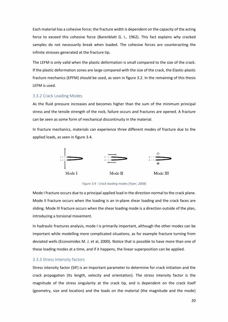
20
Each material has a cohesive force; the fracture width is dependent on the capacity of the acting
force to exceed this cohesive force (Barenblatt G. I., 1962). This fact explains why cracked
samples do not necessarily break when loaded. The cohesive forces are counteracting the
infinite stresses generated at the fracture tip.
The LEFM is only valid when the plastic deformation is small compared to the size of the crack.
If the plastic deformation zones are large compared with the size of the crack, the Elastic-plastic
fracture mechanics (EPFM) should be used, as seen in figure 3.2. In the remaining of this thesis
LEFM is used.
3.3.2 Crack Loading Modes
As the fluid pressure increases and becomes higher than the sum of the minimum principal
stress and the tensile strength of the rock, failure occurs and fractures are opened. A fracture
can be seen as some form of mechanical discontinuity in the material.
In fracture mechanics, materials can experience three different modes of fracture due to the
applied loads, as seen in figure 3.4.
Figure 3.4 - Crack loading modes (Fjaer, 2008)
Mode I fracture occurs due to a principal applied load in the direction normal to the crack plane.
Mode II fracture occurs when the loading is an in-plane shear loading and the crack faces are
sliding. Mode III fracture occurs when the shear loading mode is a direction outside of the plan,
introducing a torsional movement.
In hydraulic fractures analysis, mode I is primarily important, although the other modes can be
important while modelling more complicated situations, as for example fracture turning from
deviated wells (Economides M. J. et al, 2000). Notice that is possible to have more than one of
these loading modes at a time, and if it happens, the linear superposition can be applied.
3.3.3 Stress Intensity factors
Stress intensity factor (SIF) is an important parameter to determine for crack initiation and the
crack propagation (Its length, velocity and orientation). The stress intensity factor is the
magnitude of the stress singularity at the crack tip, and is dependent on the crack itself
(geometry, size and location) and the loads on the material (the magnitude and the mode)

21
(Taleghani A. D., 2009). SIF are used in fracture mechanics to increase the predictions accuracy
of the near-tip stress state induced by fluid pressures and in-situ stresses.
For each crack loading mode, there is an associated stress intensity factor 𝐾𝑖. Knowing the stress
intensity factor related to each loading mode, it is possible to estimate the stress field at the
crack tip. This requires the definition of a polar coordinates system (𝑟, 𝜃), with origin defined at
the crack tip, as seen in figure 3.5.
Figure 3.5 - Schematic representation of crack tip stresses defined in polar coordinates
In polar coordinates, for a linear elastic and cracked material, the stress field is:
𝜎𝑖𝑗 = (
𝑘
√𝑟) 𝑓𝑖𝑗(𝜃) + ∑ 𝐴𝑚
∞
𝑚=0
√𝑟𝑚𝑔𝑖𝑗(𝑚)
(𝜃)
(3.19)
Where 𝜎𝑖𝑗 is the stress tensor, 𝑘 is a constant related with SIF and 𝑓𝑖𝑗 is a dimensionless tensor
function dependent on 𝜃, where 𝜃 is the angle with the x axis in the polar coordinates system.
For the higher-order terms, 𝐴𝑚 is the amplitude and a dimensionless function dependent on 𝜃.
Equation 3.19 shows that independently of the fracture geometry, the stress state is asymptotic,
tending to infinite near the crack tip (𝑟 ≈ 0).
The stress field for Mode I, at a radial distance 𝑟 of the crack tip is defined as:
𝜎𝑥𝑥 =
𝐾𝐼
√2𝜋𝑟cos
𝜃
2(1 − sin
𝜃
2sin
3𝜃
2)
(3.20)
𝜎𝑦𝑦 =
𝐾𝐼
√2𝜋𝑟cos (
𝜃
2)(1 + sin (
𝜃
2) sin (
3𝜃
2))
(3.21)
𝜏𝑥𝑦 =
𝐾𝐼
√2𝜋𝑟cos (
𝜃
2) sin (
𝜃
2) cos (
3𝜃
2)
(3.22)
And the displacement field is expressed (Fleming M. et al, 1997):

22
𝑢𝑥 =
𝐾𝐼
2𝜇 √
𝑟
2𝜋cos (
𝜃
2) [𝑘 − 1 + 2(sin (
𝜃
2)2
)]
(3.23)
𝑢𝑦 =
𝐾𝐼
2𝜇 √
𝑟
2𝜋cos (
𝜃
2) [𝑘 + 1 − 2(cos (
𝜃
2)2
)]
(3.24)
Where 𝑢𝑖 are the displacements and 𝜇 is the shear modulus.
3.3.4 Griffith energy balance equation
As stated before, the stress intensity in the near-tip region tends to infinite, however it is
observed that cracked samples do not necessarily break when loaded. Griffith (1920) proposed
a new theory based on the first law of thermodynamics, and on the postulate that when a
system goes from a non-equilibrium state to equilibrium, there is a net decrease in energy.
Griffith (1920) got satisfactory results for materials obeying the Hooke's law (linear elastic
materials). Before Griffith, it was though that the strength of a fracture was independent of its
size. Griffith examined fractures of various sizes in a brittle material (glass), and found that as
larger is the sample, the lower is the resistance. This fact became known as "size effect"; i.e. the
larger the sample the more likely the material is to crack, hence lower resistance ((Anderson T.
L., 2005) and (Ahmed A., 2009)).
Griffith's theory admits that the crack is represented by an elliptical shape, as seen in Figure 3.6.
The crack propagates when the elastic potential energy supplied overcomes the crack growth
resistance (the energy required to form a new surface cracking, i.e. the energy required to break
the cohesion between the front atoms the crack).
The total energy of the system,Ψ, consists of two parts (Fischer-Cripps et Anthony C., 2007):
The elastic potential energy supplied by the material strain and external loads applied
to the system Π
The work required to form the crack surface 𝑊𝑠
The total energy must decrease or remain constant for a crack to form or to enable its
propagation. The formation of the crack (and the two new surfaces), when the surface energy
of the material 𝛾𝑠 is exceeded, relaxes the stresses and the stored potential elastic strain energy,
Π reduces near the crack faces.

23
Figure 3.6 - Griffith energy balance for an elliptical shape crack
The Griffith energy balance for an incremental increase in the crack area 𝜕𝐴, under equilibrium
conditions, as seen in figure 3.6, can be expressed as:
𝜕Ψ
𝜕𝐴=
𝜕Π
𝜕𝐴+
𝜕𝑊𝑠
𝜕𝐴= 0
(3.25)
For an elliptical crack, the following stress analysis can be done ((Ahmed A., 2009) and (Griffith
A. A., 1921)):
Π = Π0 −
𝜋𝜎2𝑎2𝐵
𝐸
(3.26)
Where Π0 is the potential energy of an uncracked plate and B is the plate thickness. Since the
formation of a crack requires the creation of two surfaces, the work required to form the crack
surface, 𝑊𝑠 is given by the following expression:
𝑊𝑠 = 4𝑎𝐵𝛾𝑠
(3.27)
Where 𝛾𝑠 is the surface energy of the material. Thus,
𝜕Π
𝜕𝐴= −
𝜋𝜎2𝑎
𝐸
(3.28)
And,
𝜕𝑊𝑠
𝜕𝐴= 2𝛾𝑠
(3.29)
Solving for the fracture stress,
𝜎𝑓 = √2𝐸𝛾𝑠
𝜋𝑎
(3.30)
Where 𝜎𝑓 is the critical fracture tangential stress to cause the fracture initiation. As mentioned
before, the expression above was derived assuming that the fracture and the surrounding media

24
are isotropic linear elastic materials. This equation can be modified to account for the fracture
elastic-plastic characteristic, as follows ((Orwan E., 1948) and (Anderson T. L., 2005)):
𝜎𝑓 = √2𝐸(𝛾𝑠 + 𝛾𝑝)
𝜋𝑎
(3.31)
Where 𝛾𝑝 is the plastic energy of the material.
3.3.5 The energy release rate – 𝐺
Irwin (1948) proposes an approach to describe the conditions of fracture initiation, which is
essentially equivalent to the Griffith model. Irwin (1948) defined the energy release ratio, G, as
a measure of the energy available for increasing the extent of the crack:
𝐺 = −
𝜕Π
𝜕𝐴
(3.32)
G is the rate of potential energy variation with crack area. Since G is obtained from the derivative
of a potential, it is called the crack extension force or the crack driving force (Oliveira F., 2013).
For linear elastic material under loading mode I, this scalar entity can be expressed as:
𝐺 =
𝐾𝐼2
𝐸′
(3.33)
Where for a plane stress 𝐸 = 𝐸′ and for a plane strain 𝐸′ =𝐸
1−𝜐2 .
3.3.6 Failure Criteria
The critical value of the stress intensity factor, 𝐾𝑐, also known as fracture toughness
(Economides M. J. et al, 2000), determines the material resistance to the fracture initiation. At
a microscopically and macroscopically level, the fracture toughness of a material exists due to
the strength of connection bonds between constituent particles and the size and number of
natural flaws in the material. Fracture toughness is widely used to describe fracture propagation
through rock, and it appears to be a valid predictor of fracture propagation in cohesive soils. In
rock, fracture toughness values are typically on the order of 0,5 − 3 𝑀𝑃𝑎√𝑚.
The propagation criterion, under mode I loading condition, assumes that the propagation will
continue as far as the criterion for fracture advance is:
𝐾𝐼𝐶 ≤ 𝐾𝐼
(3.34)
On the other hand, the fracture will cease propagation when:
𝐾𝐼𝐶 > 𝐾𝐼 (3.35)

25
Fracture toughness is not a material property, but depends on the problem geometry, as
discussed later in Chapter 5. The failure criteria may also be written in terms of the energy
release rate for LEFM, once there is a direct relationship between both.
3.3.7 J-Integral
To study crack growth, Rice (1977) developed an energy related method, based on a contour
integral, to calculate the stress intensity factors. Even if there is plasticity, this method can be
used in brittle and ductile materials. In LEFM, the value of the J-integral in a contour surrounding
the crack tip is exactly the energy release rate, G and thus is directly related to the stress
intensity factors of the crack (Li S. et Simkins Jr. D. C., 2002).
The J-Integral can be defined as a line integral around the crack tip, invariant of the adopted
path since it starts on the underside and ends in the upper surface of the crack as seen in Figure
3.7. The path is represented by arrows counter-clockwise (Anderson T. L., 2005).
Figure 3.7 - Schematic representation of the 2D line J-Integral (Dassault Systémes, 2015)
The J-integral thus provided an alternative approach to calculate the G or K (stress intensity
factors). The Rice’s integral in its original form can be expressed as:
𝐽 = ∫ (𝑊𝜕𝑦 − 𝑇
𝜕𝑢
𝜕𝑥𝜕𝑠)
Γ
(3.36)
Where Γ is a curve surrounding the crack tip, 𝑇 is the traction vector defined according to
outward normal along Γ, 𝑇𝑖 = 𝜎𝑖𝑗𝑛𝑗 , 𝑢 is the displacement vector, and 𝜕𝑠 is an element of an
arc with total length Γ.
𝑊 is the strain energy density, given by:
𝑊(휀) = ∫ 𝜎𝑖𝑗𝛿휀𝑖𝑗
𝜀
0
(3.37)
As mentioned above, the J-integral is numerically equal to the energy release rate in LEFM,
therefore it is also related to the stress intensity factor through the following expression:
𝐽 =
1
8𝜋𝐾𝑇𝐵−1𝐾
(3.38)
26
Where 𝐾 = [𝐾𝐼 , 𝐾𝐼𝐼 , 𝐾𝐼𝐼𝐼]𝑇 and 𝐵 is the pre-logarithmic energy factor tensor. For homogeneous
and isotropic materials, the expression can be simplified as:
𝐽 =
1
𝐸′(𝐾𝐼
2 + 𝐾𝐼𝐼2) +
1
2𝐺𝐾𝐼𝐼𝐼
3
(3.39)
3.4 Fluid Mechanics
3.4.1 Material behavior and constitutive equations
Basic concepts
Fluid mechanics in an important element in the application of fracturing techniques
(Economides M. J. et al, 2000). The two basic fluid mechanics variables, injection rates (𝑞𝑖) and
fluid viscosity (µ) affect pressure, control the displacement rates of the proppant and have an
important role when controlling the fluid loss to the formation.
Flow is usually defined as the relative sliding of parallel layers. The external forces can be
originated from pressure and/or gravity differentials (Poiseuille flow) or from torque (Couette
flow). As a reaction, in order to keep the equilibrium of the system, in the opposite direction,
the shear stress has the magnitude:
𝜏 = 𝜇 × �̇�
(3.40)
Where 𝜇 is the fluid apparent viscosity and �̇� is the shear rate.The shear rate is defines as:
𝛾 ̇ =
∆𝑢
∆𝑦
(3.41)
The shear stress/shear rate relationship expressed in an algebraic form is the rheological
constitutive equation and it is graphically represented as a rheological curve. The shear
stress/shear rate relationship is a material property and it is independent of the flow’s geometry.
If the flow rates are extremely high, the application of the concept of parallel sliding layers is
impracticable due to the appearance of more complex flow movements (turbulence) (Valkó P.
et Economides M. J., 1995).
Rheological models
Fluids can be classified in terms of the shape of their rheological empirical curve, as shown in
Figure 3.8.
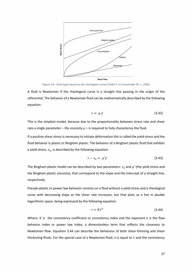
27
Figure 3.8 - Fluid types based on the rheological curves (Valkó P. et Economides M. J., 1995)
A fluid is Newtonian if the rheological curve is a straight line passing in the origin of the
referential. The behavior of a Newtonian fluid can be mathematically described by the following
equation:
𝜏 = 𝜇 �̇�
(3.42)
This is the simplest model, because due to the proportionality between stress rate and shear
rate a single parameter – the viscosity 𝜇 – is required to fully characterize the fluid.
If a positive shear stress is necessary to initiate deformation this is called the yield stress and the
fluid behavior is plastic or Bingham plastic. The behavior of a Bingham plastic fluid that exhibits
a yield stress, 𝜏0, is described by the following equation:
𝜏 − 𝜏0 = 𝜇′�̇�
(3.43)
The Bingham plastic model can be described by two parameters: 𝜏0and 𝜇′ (the yield stress and
the Bingham plastic viscosity), that correspond to the slope and the intercept of a straight line,
respectively.
Pseudo-plastic or power law behavior consists on a fluid without a yield stress and a rheological
curve with decreasing slope as the shear rate increases, but that plots as a line in double
logarithmic space, being expressed by the following equation:
𝜏 = 𝐾�̇�𝑛
(3.44)
Where, 𝐾 is the consistency coefficient or consistency index and the exponent 𝑛 is the flow
behavior index or power law index, a dimensionless term that reflects the closeness to
Newtonian flow. Equation 3.44 can describe the behaviour of both shear-thinning and shear
thickening fluids. For the special case of a Newtonian fluid, n is equal to 1 and the consistency

28
index 𝐾 corresponds then to the viscosity of the fluid, 𝜇. When 𝑛 is less than 1 the fluid is shear-
thinning and when 𝑛 is higher than1 the fluid is shear-thickening in nature.
For power law fluids the apparent viscosity, which is defined as the ratio between applied shear
stress and the shear rate, is given by the following equation:
𝜇𝑎 = 𝐾�̇�𝑛−1
(3.45)
Polymeric solutions and melts are examples of power-law fluids. Some drilling fluids and cement
slurries, depending on their formulation, may also exhibit shear thinning power-law behavior.
When there is a yield stress and this is included in the power law model, the model is then known
as the Herschel–Bulkley model, given by the following equation:
𝜏 − 𝜏0 = 𝐾𝐻�̇�𝑛𝐻
(3.46)
Where, 𝑛 is the flow behavior index, 𝐾𝐻 is the consistency index, and 𝜏0 is yield stress. The yield
stress may be understood as a threshold for large scale yielding and thus an engineering reality
and plays an important role.
Dilatant behavior is characterized by a monotonic increase in the slope of the rheological curve
with shear rate (Montegomery C., 2013). Most fluids do not conform exactly to any of these
models, but their behavior can be adequately described by one of them. Several other
constitutive equations have been proposed and can be found in the literature to reproduce real
fluid behavior ((Valkó P. et Economides M. J., 1995) and (Rao M. A., 2014)).
3.4.2 Fluid Flow – Hydraulic transport in rocks
Darcy law
Assuming Darcy´s is valid, the relationship between the flow velocity vector 𝑞 and the pore
pressure 𝑃𝑝, under the assumption that the flow velocity vector depends only on the pressure
gradient in one direction, is described by:
𝑞 =
𝑘
𝜇𝑖 =
𝑘
𝜇 ∆𝑃𝑝
∆𝑙=
𝑄
𝐴
(3.47)
Where 𝑄 is the flow rate, 𝐴 is the cross section area of the fracture, 𝑘 is the intrinsic
permeability, 𝜇 is the viscosity and 𝑖 is the pressure gradient along the distance ∆𝑙.
The following assumptions have to be met for the Darcy’s law to apply:
Inertial forces can be neglected.
Steady state flow conditions are valid.
The medium is isotropic and fully saturated with a single phase fluid.
The fluid is homogeneous and contains only one phase.
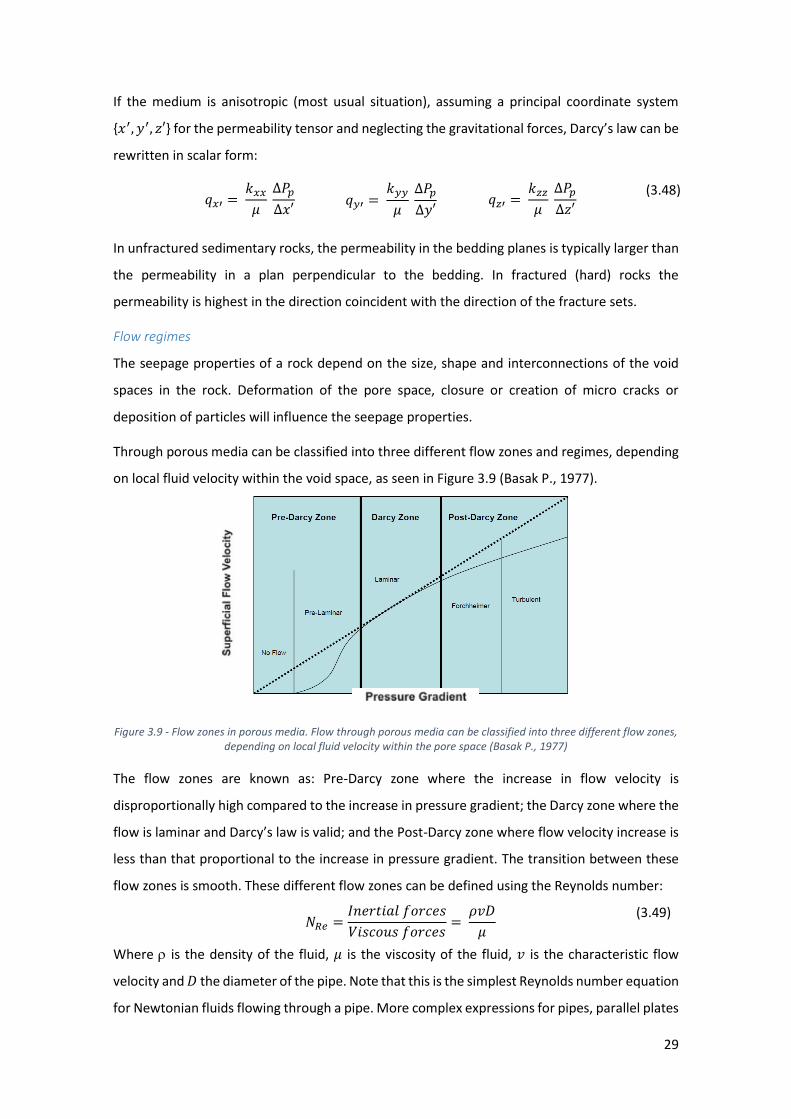
29
If the medium is anisotropic (most usual situation), assuming a principal coordinate system
{𝑥′, 𝑦′, 𝑧′} for the permeability tensor and neglecting the gravitational forces, Darcy’s law can be
rewritten in scalar form:
𝑞𝑥′ =
𝑘𝑥𝑥
𝜇 ∆𝑃𝑝
∆𝑥′
𝑞𝑦′ = 𝑘𝑦𝑦
𝜇 ∆𝑃𝑝
∆𝑦′
𝑞𝑧′ = 𝑘𝑧𝑧
𝜇 ∆𝑃𝑝
∆𝑧′
(3.48)
In unfractured sedimentary rocks, the permeability in the bedding planes is typically larger than
the permeability in a plan perpendicular to the bedding. In fractured (hard) rocks the
permeability is highest in the direction coincident with the direction of the fracture sets.
Flow regimes
The seepage properties of a rock depend on the size, shape and interconnections of the void
spaces in the rock. Deformation of the pore space, closure or creation of micro cracks or
deposition of particles will influence the seepage properties.
Through porous media can be classified into three different flow zones and regimes, depending
on local fluid velocity within the void space, as seen in Figure 3.9 (Basak P., 1977).
Figure 3.9 - Flow zones in porous media. Flow through porous media can be classified into three different flow zones, depending on local fluid velocity within the pore space (Basak P., 1977)
The flow zones are known as: Pre-Darcy zone where the increase in flow velocity is
disproportionally high compared to the increase in pressure gradient; the Darcy zone where the
flow is laminar and Darcy’s law is valid; and the Post-Darcy zone where flow velocity increase is
less than that proportional to the increase in pressure gradient. The transition between these
flow zones is smooth. These different flow zones can be defined using the Reynolds number:
𝑁𝑅𝑒 =
𝐼𝑛𝑒𝑟𝑡𝑖𝑎𝑙 𝑓𝑜𝑟𝑐𝑒𝑠
𝑉𝑖𝑠𝑐𝑜𝑢𝑠 𝑓𝑜𝑟𝑐𝑒𝑠=
𝜌𝑣𝐷
𝜇
(3.49)
Where is the density of the fluid, 𝜇 is the viscosity of the fluid, 𝑣 is the characteristic flow
velocity and 𝐷 the diameter of the pipe. Note that this is the simplest Reynolds number equation
for Newtonian fluids flowing through a pipe. More complex expressions for pipes, parallel plates

30
and ellipses assuming other rheological models can be found in the literature ((Economides M.
J. et al, 2000) and (Valkó P. et Economides M. J., 1995)).
The most typical 𝑁𝑅𝑒 threshold values are set in Table 3.1:
Table 3.1 - Reynolds number values associated with the different flow regimes (Amao A. M., 2007)
Zone Flow Regime Reynolds Number
Pre-Darcy No flow 𝑁𝑅𝑒 < 1000 Pre laminar flow
Darcy Laminar flow 𝑁𝑅𝑒 < 2300
Post-Darcy Forcheimer flow 2300 < 𝑁𝑅𝑒 < 4000 Turbulent flow 𝑁𝑅𝑒 > 4000
A reasonable explanation why the flow does not follow Darcy’s law for very small pressure
gradients can be given by the boundary layer theory (Schlichting H. et Gersten K., 2000). Because
of the liquid-solid interactions, the viscous forces at the interfaces/surface are much stronger
than in the center of the pores. This effect leads to low to null velocities in the fracture surfaces,
high velocities in the gravity center of the fracture and a subsequent creation of vortices
according to the theory of laminar instability (Tani I., 1962).
With increasing pressure gradient (e.g. higher flow rate), the small pores start to take part in the
flow leading to an apparent increase of permeability. In the Post-Darcy zone (high flow rates),
inertial forces begin to control the flow velocity and the flow field is not laminar.
At the reservoir scale, the various flow regimes illustrated in Figure 3.9 can be found in the near
field and the far field, around the borehole and hydraulic fracture, respectively. Near and within
the wellbore, the fracture flow can be turbulent. In the rock mass surrounding the wellbore or
the fracture, flow is likely to be laminar and described by the Darcy’s law. At a sufficient distance
from the borehole or fracture, the pressure gradient decreases potentially below the Pre-Darcy
threshold resulting in a reduction in the apparent permeability (Basak P., 1977).
Forchheimer Equation and Non-Darcy Flow Correction
In 1901, Philippe Forchheimer discovered that, at sufficiently high velocity, the relationship
between flow rate and potential gradient is non-linear, and that this non-linearity increases with
flow rate. Initially this non-linearity was attributed to increased turbulence in the fluid flow;
however it is now known that this non-linearity is due to inertial effects in the porous media.
The pressure drop at high velocities, in the Forcheimer flow regime is given by Forchheimer
empirical equation:
𝜕𝑝
𝜕𝑥=
𝜇
𝑘𝑞 + 𝛽𝜌𝑣2
(3.50)
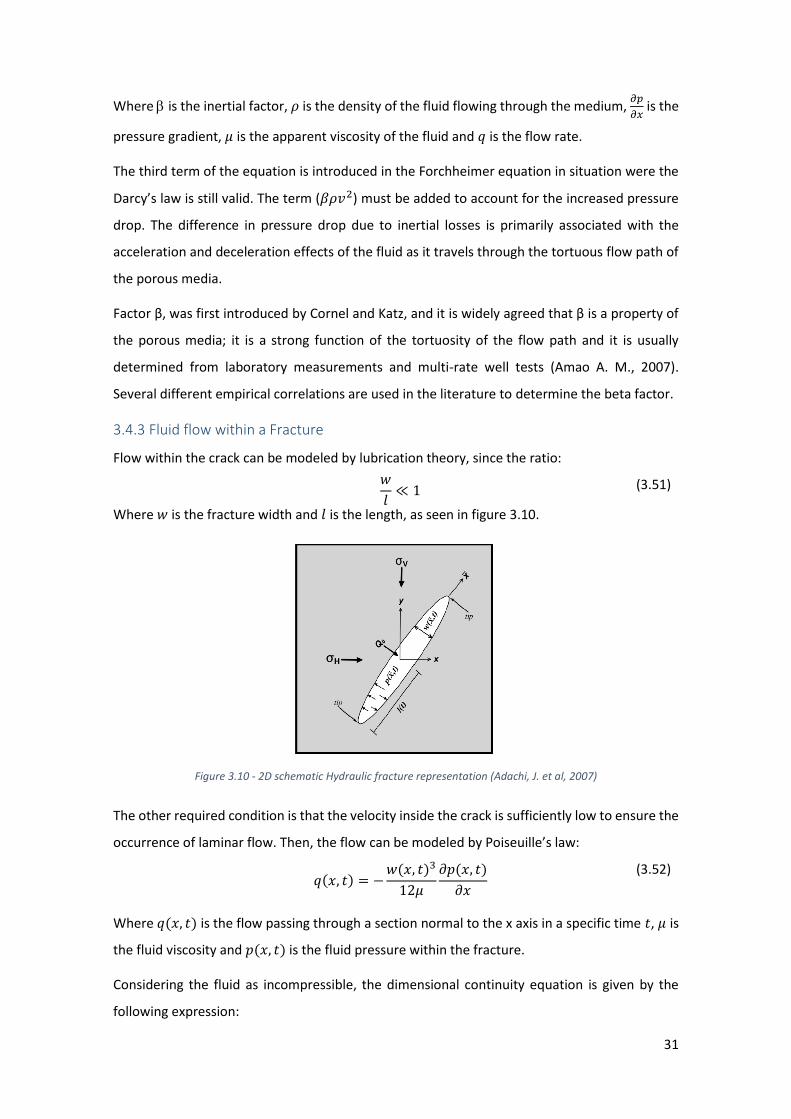
31
Where is the inertial factor, 𝜌 is the density of the fluid flowing through the medium, 𝜕𝑝
𝜕𝑥 is the
pressure gradient, 𝜇 is the apparent viscosity of the fluid and 𝑞 is the flow rate.
The third term of the equation is introduced in the Forchheimer equation in situation were the
Darcy’s law is still valid. The term (𝛽𝜌𝑣2) must be added to account for the increased pressure
drop. The difference in pressure drop due to inertial losses is primarily associated with the
acceleration and deceleration effects of the fluid as it travels through the tortuous flow path of
the porous media.
Factor β, was first introduced by Cornel and Katz, and it is widely agreed that β is a property of
the porous media; it is a strong function of the tortuosity of the flow path and it is usually
determined from laboratory measurements and multi-rate well tests (Amao A. M., 2007).
Several different empirical correlations are used in the literature to determine the beta factor.
3.4.3 Fluid flow within a Fracture
Flow within the crack can be modeled by lubrication theory, since the ratio:
𝑤
𝑙≪ 1 (3.51)
Where 𝑤 is the fracture width and 𝑙 is the length, as seen in figure 3.10.
Figure 3.10 - 2D schematic Hydraulic fracture representation (Adachi, J. et al, 2007)
The other required condition is that the velocity inside the crack is sufficiently low to ensure the
occurrence of laminar flow. Then, the flow can be modeled by Poiseuille’s law:
𝑞(𝑥, 𝑡) = −
𝑤(𝑥, 𝑡)3
12𝜇
𝜕𝑝(𝑥, 𝑡)
𝜕𝑥
(3.52)
Where 𝑞(𝑥, 𝑡) is the flow passing through a section normal to the x axis in a specific time 𝑡, 𝜇 is
the fluid viscosity and 𝑝(𝑥, 𝑡) is the fluid pressure within the fracture.
Considering the fluid as incompressible, the dimensional continuity equation is given by the
following expression:
32
Combining equations 3.52 e 3.53, the Reynolds equation can be retrieved. Reynolds equation is
expressed as:
𝛿𝑤(𝑥, 𝑡)
𝛿𝑡=
𝛿
𝛿𝑥(𝑤(𝑥, 𝑡)3
12𝜇
𝛿𝑝(𝑥, 𝑡)
𝛿𝑥) + 𝛿(𝑥0)𝑄0
(3.54)
Where 𝛿(𝑥𝑜) is the delta Dirac function of the injection at point 𝑥0 and 𝑄0 is the fluid injection
in the fracture at point 𝑥0 .
Two boundary conditions are essential to predict the fluid flow inside fracture:
𝑞(0+, 𝑡) =
𝑄0
2
(3.55)
𝑞(𝑙, 𝑡) = 0 (3.56)
Equation 3.55 is a consequence of fracture symmetry in relation to the injection point and
Equation 3.56 imposes the impermeability of the rock mass (zero flow along the perimeter of
the fracture (assuming a no fluid leak-off situation).
To ensure the existence and uniqueness of the solution to the Reynolds equation with the
specified boundary conditions, it is necessary to impose the condition of mass conservation:
∫ 𝑤(𝑥, 𝑡)𝛿𝑥 = ∫𝑄(𝑡)𝛿𝑡
𝑡
0
𝑙(𝑡)
0
(3.57)
𝛿𝑤(𝑥, 𝑡)
𝛿𝑡+
𝛿𝑞(𝑥, 𝑡)
𝛿𝑥= 0
(3.53)

33
4. Numerical methods for fracture analysis
4.1 Introduction
The finite element method (FEM) is a capable method to model fractures; however, some effects
require a locally refined mesh. As a consequence, there is an increase in terms of nodal quantity
and consequently in the simulation running time.
The fracture propagation analysis is a challenge for traditional FEM, since it requires the mesh
discretization to be compatible with the discontinuity which requires re-meshing at each time
step, increasing the computational costs, loss of accuracy and convergence.
As a solution, the extended finite element method (XFEM) allows to model discontinuities and
singularities independently on the initial mesh. XFEM is based on the principles of partition of
unity and enriched local shape functions for strong discontinuities.
This chapter provides a description of the two numerical methods, highlighting their capabilities
and limitations.
4.2 Finite Element Method (FEM)
The aim of the finite element method is to calculate the field of stresses and deformations across
the problem domain. In the FEM the analysis domain is divided into elements and the unknowns,
for a traditional formulation, are the values of the displacements at the nodes, and all the
remaining quantities can be expressed as a function of the nodal displacements.
The formulation of the finite element method to problems with a two dimensional geometry is
obtained from a solution represented by 𝑢(𝑥) = (𝑢𝑥 , 𝑢𝑦), where 𝑢(𝑥) is the displacement field,
which can be expressed by the following expression:
𝑢(𝑥) = ∑𝑁𝑖(𝑥)𝑢𝑖
𝑛
𝑖=1
(4.1)
Where 𝑁𝑖(𝑥) are the shape functions, n the number of nodes in the element and 𝑢𝑖 are the
nodal displacement values, which are obtained by solving the following equation:
𝑀𝑢𝑖 = 𝐹
(4.2)
Where 𝐹 is the external loads/forces vector and 𝑀 is the stiffness matrix, obtained through the
virtual work theorem.
For a two-dimensional problem, equation 4.1 may be represented as:
[𝑢𝑥
𝑢𝑦] = ∑[
𝑁𝑖 00 𝑁𝑖
]
𝑛
𝑖=1
[𝑢𝑥
𝑖
𝑢𝑦𝑖 ]
(4.3)

34
The application of the FEM requires the domain to be discretized, through the division of the
continuum into elements of known geometries (typically quadrilateral or trilateral shapes), and
all these elements are interconnected through nodes. Then, interpolation shape functions
should be selected (Mohammadi S., 2008).
4.2.1 Virtual work theorem
The virtual work theorem postulates that when the body is subjected to a set of forces
𝑓 (Figure 4.1) the energy dissipated during the body deformation is equal to the work of the
external forces, which is expressed by the following expression:
∫ (𝜕휀)𝑇𝜎𝜕Ω = ∫ (𝜕𝑢)𝑇𝑓𝑡𝜕Ω + ∫ (𝜕𝑢)𝑇𝑡𝜕Γ
Γ𝑡ΩΩ
(4.4)
Where 𝑓𝑡 represents the volume forces, 𝑡 represents the superficial tensile forces, Ω the
domain, Γ𝑡 represents the contour line of the domain Ω , and 𝜕휀 𝑎𝑛𝑑 𝜕𝑢 are the strain and
displacements vectors, respectively.
Figure 4.1 - FEM domain for application of virtual work principle (adapted from (Mohammadi S., 2008))
The expressions for the displacement, strains and their virtual components can be expressed in
terms of the nodal displacements:
휀 = ∑𝐵𝑖𝑢𝑖
𝑚
𝑖=1
(4.5)
𝜕휀 = ∑𝐵𝑖𝜕𝑢𝑖
𝑚
𝑖=1
(4.6)
𝑢 = ∑𝑁𝑖𝑢𝑖
𝑚
𝑖=1
(4.7)
𝜕𝑢 = ∑𝑁𝑖𝜕𝑢𝑖
𝑚
𝑖=1
(4.8)
Where 𝑁𝑖 represents the global matrix of the shape functions and 𝐵𝑖 the global matrix of the
derivatives of the shape function, expressed as:

35
𝐵𝑖 =
[ 𝜕𝑁𝑖
𝜕𝑥0
0𝜕𝑁𝑖
𝜕𝑦𝜕𝑁𝑖
𝜕𝑦
𝜕𝑁𝑖
𝜕𝑥 ]
(4.9)
When Equations 4.5 to 4.8 are substituted in Equation 4.4, then the virtual work for each
element can be expressed as:
∫ (𝐵𝑖)
𝑇𝜎𝜕Ω = ∫ (𝑁𝑖)𝑇𝑓𝑡𝜕Ω
Ω
+ ∫ (𝑁𝑖)𝑇𝑡𝜕Γ
ΓΩ
(4.10)
The displacements of the continuous medium can be calculated as a function of the nodal
displacements. The contribution of the displacement of each finite element can be expressed
as:
𝑢(𝑒) = ∑𝑁𝑖
(𝑒)𝑢𝑖
(𝑒)
𝑛
𝑖=1
(4.11)
Due to the complexity of the elements in study, the shape functions are mapped in a local
coordinate system, as seen in figure 4.2 (Caldeira L. et Cardoso R., 2013).
Figure 4.2 - Mapping of a Finite element in global and local coordinates (Mohammadi S., 2008)
The discrete volume of each finite element can be expressed as:
𝛿Ω(𝑒) = 𝐷𝑒𝑡𝐽(𝑒)𝜕𝜉𝜕𝜂
(4.12)
Where 𝜕𝜉 𝑎𝑛𝑑 𝜕𝜂 are the local coordinates and 𝐽(𝑒) is the jacobian matrix of each finite element,
defined as:
𝐽(𝑒) =
[ 𝜕𝑥
𝜕𝜉
𝜕𝑦
𝜕𝜂𝜕𝑥
𝜕𝜂
𝜕𝑦
𝜕𝜂]
=
[ ∑
𝜕𝑁𝑖(𝑒)
𝜕𝜉
𝑛
𝑖=1
𝑥𝑖(𝑒)
∑𝜕𝑁𝑖
(𝑒)
𝜕𝜉
𝑛
𝑖=1
𝑦𝑖(𝑒)
∑𝜕𝑁𝑖
(𝑒)
𝜕𝜂
𝑛
𝑖=1
𝑥𝑖(𝑒)
∑𝜕𝑁𝑖
(𝑒)
𝜕𝜂
𝑛
𝑖=1
𝑦𝑖(𝑒)
]
(4.13)
Finally, the stiffness matrix 𝐾𝑒 of an element with volume Ω𝑒 can be determined in local
coordinates, as:

36
𝐾𝑒 = ∫ ∫ 𝐵𝑖
(𝑒)𝑇𝐷(𝑒)𝐵𝑗
(𝑒)𝐷𝑒𝑡𝐽(𝑒)𝜕𝜉𝜕𝜂
+1
−1
+1
−1
(4.14)
Where 𝐷(𝑒) is the material constitutive matrix (Caldeira L. et Cardoso R., 2013). Then the
element stiffness matrixes of the various elements need to be assembled to give the global
stiffness matrix 𝐾, giving the final global relation between global force, displacement, and
stiffness matrices (Anderson T. L., 2005):
[𝐾][𝑢] = [𝐹]
(4.15)
Where [𝐾] is the stiffness matrix, [𝑢] is the global displacement vector and [𝐹] is the global
force vector.
4.2.2 Discretization of the elements
As explained later in the Chapter, in the XFEM, fracture is modeled independent of mesh
configuration and element type. This means that no re-meshing is required and fractures do not
need to be aligned with element boundaries. However, the type of element and mesh
discretization have effects on simulation convergence and results (Sepehri J., 2014).
The discretization by finite elements for the analysis of a propagating crack in the context of
computational fracture mechanics, recommends biquadratic Lagrangian elements of eight
nodes for two-dimensional problems and the twenty nodes element for three-dimensional
problems, as seen in figure 4.3.
2 dimensional element of 8 nodes 3 dimensional element of 20 nodes Figure 4.3 - Finite elements discretization for 2D and 3D classical fracture mechanics ( (Mohammadi S., 2008)
As one of the objectives of the element discretization is to analyze the stress and strain at the
crack tip (by the calculation of stress intensity factors), once the stresses and strains vary in the
form 1
𝑟 at the crack tip, is possible to show that triangular geometries introduces more accurate
and satisfactory results than quadrilateral elements (Barsoum R. S., 1976).
To capture the behavior of the singularity, quadrilateral elements are degenerated into
triangular geometry, as seen in Figure 4.4. In quadrilateral elements the singularity is only found
inside the element, whereas in the triangular elements it can be located inside and on the
contour of the element. This is a simple and effective way to build elements that incorporate in

37
their strain field the singularity 1
𝑟. In elastic problems, the nodes at the crack tip are moved to
the 1
4 points (quarter-point). This modification is necessary to introduce a
1
𝑟 strain singularity in
the element, which brings numerical accuracy (Oliveira F., 2013).
Figure 4.4 - Construction of the spider-web mesh, based on the degeneration of quadrilateral elements in triangular elements (Dassault Systémes, 2013)
As seen in figure 4.4, the spider web configuration near the crack tip is the most efficient mesh
discretization to analyze the crack tip stress intensity factors.
4.3 Partition of the Unity
The theory of partition of unity is an important tool for fracture modelling. The word unity stands
for the constant shape function, 𝜂𝑖 , equal to the unity on some given space 𝑋. These shape
functions form a partition of unity, as seen in figure 4.5.
Figure 4.5 - Partition of unity concept (Wikipedia, 2015) - 𝑁𝑖,𝑖 = 𝜂𝑖
In a mathematical formulation, Partition of unity is a set ℝ ∈ [0,1] of continuous functions from
𝑋 such that for every point, 𝑥 ∈ 𝑋 the following conditions are verified (Robbin J. W., 2014):
∑ 𝜂𝑖𝑛𝑖=1 = 1 , ∀ 𝑥 𝜖 𝑋
At any given point 𝑥 all but one finite number of the functions are equal to 0
It can be shown that for any arbitrary function 𝜓(𝑥), the following property is automatically
satisfied:

38
∑𝜂𝑖(𝑥)𝜓(𝑥)
𝑛
𝑖=1
= 𝜓(𝑥) (4.16)
Where 𝜂𝑖 is a constant shape function and 𝜓(𝑥) is an arbitrary function.
This formalism is the basis of the XFEM. By appropriately choosing the function 𝜓(𝑥) for each
node, the computation time may be reduced (McNary M. J., 2009).
4.3.1 Partition of Unity Finite Element Method
To improve a finite element approximation, the enrichment procedure may be applied. The
methodology followed in the partition of unity finite element method (PUFEM) is defined using
the classical finite element shape functions 𝑁𝑖. For a general point 𝑥 within a finite element, the
displacement field is given by:
𝑢(𝑒)(𝑥) = ∑𝑁𝑖(𝑥)𝑢𝑖(𝑥) + ∑∑𝑁𝑖
𝑚
𝑗=1
𝑛
𝑖=1
𝑛
𝑖=1
(𝑥)𝑝𝑗(𝑥)𝑎𝑖𝑗 = ∑𝑁𝑖(𝑥) (𝑢𝑖(𝑥) + ∑ 𝑝𝑗(𝑥)𝑎𝑖𝑗
𝑚
𝑘=1
)
𝑛
𝑖=1
(4.17)
Where 𝑢(𝑒) is the element displacement, 𝑝𝑗(𝑥) are the enrichment functions, 𝑎𝑖𝑗 are the
additional unknowns or degrees of freedom associated to the enriched solution and 𝑛 and
𝑚 are the total number of nodes of finite elements and the number of enrichment
functions 𝑝𝑗, respectively.
The approximation is clearly a partition of unity. As a result, a compatible solution is guaranteed.
Examining the approximate solution for a typical enriched node 𝑥𝑖 , equation 4.17 can be written
as:
𝑢(𝑒)(𝑥𝑖) = 𝑢𝑖 + ∑𝑝𝑗(𝑥𝑖)𝑎𝑖𝑗
𝑚
𝑘=1
(4.18)
Which is not a possible solution because it does not respect the condition (𝑢(𝑒)(𝑥𝑖) = 𝑢𝑖). A
slightly modified expression is required for the enriched displacement field to satisfy the
interpolation at nodes:
𝑢(𝑒)(𝑥) = ∑𝑁𝑖(𝑥) (𝑢𝑖(𝑥) + ∑ (𝑝𝑗(𝑥) − 𝑝𝑗(𝑥𝑖)) 𝑎𝑖𝑗
𝑚
𝑘=1
)
𝑛
𝑖=1
(4.19)
Which ensures 𝑢(𝑒)(𝑥𝑖) = 𝑢𝑖 .
4.3.2 Generalized Finite element method
In the generalized FEM, different shape functions are used for the classical and enriched parts
of the approximation, consisting in an advance in relation to the partition of unity FEM and
allowing a great improvement in finite element discretization. Generalized FEM can be
expressed as:

39
𝑢(𝑒)(𝑥) = ∑𝑁𝑖(𝑥)𝑢𝑖(𝑥) + ∑∑𝑁�̅�
𝑚
𝑗=1
𝑛
𝑖=1
𝑛
𝑖=1
(𝑥)𝑝𝑗(𝑥)𝑎𝑖𝑗 (4.20)
Where �̅�𝑖(𝑥) are the new set of shape functions associated with the enrichment part of the
approximation. For the same reason explained before, equation 4.20 should be modified as
follows:
𝑢(𝑒)(𝑥) = ∑𝑁𝑖(𝑥)𝑢𝑖(𝑥) + ∑∑𝑁�̅�
𝑚
𝑗=1
𝑛
𝑖=1
𝑛
𝑖=1
(𝑥) (𝑝𝑗(𝑥) − 𝑝𝑗(𝑥𝑖)) 𝑎𝑖𝑗
(4.21)
4.4 Extended Finite Element Method (XFEM)
The XFEM method consists in a mesh of finite elements which is independent of the
discontinuity. This formulation takes off the need to define a new mesh configuration
(remeshing) for the simulation of crack propagation, by opposition to the classical FEM.
Therefore, the same mesh is used for all time steps during crack propagation.
The XFEM is based on the introduction of additional degrees of freedom, which are established
in the nodes of the elements that are intersected by the crack geometry, as seen in figure 4.6.
These extra degrees of freedom in combination with special shape functions allow extra
accuracy in modeling the crack.
=
Superposition of mesh with the discontinuity Enriched nodes in the mesh
Figure 4.6 - Definition of the enriched nodes in a mesh of finite elements (Duarte A. et Simone A., 2012)
In contrast to partition of unity FEM and generalized FEM, where the enrichments are usually
employed on a global level and over the entire domain, the extended finite element method
adopts the same procedure but at local level.
This is a considerable computational advantage as it is equivalent to enriching only nodes close
to the crack tip, an important step for the extended finite element solution.
Consider 𝑥, a point in a finite element that is intersected by a crack. To calculate the
displacement at point 𝑥 located within the domain, the following approximation is utilized in
XFEM:
𝑢(𝑒)(𝑥) = 𝑢𝐹𝐸𝑀 + 𝑢𝐸𝑛𝑟𝑖𝑐ℎ𝑒𝑚𝑒𝑛𝑡 = ∑𝑁𝑖(𝑥)𝑢𝑖(𝑥) + ∑𝑁𝑗
𝑚
𝑗=1
𝑛
𝑖=1
(𝑥)𝜓(𝑥)𝑎𝑗 (4.22)

40
Where 𝑢𝑖 is the vector of nodal degrees of freedom, 𝑎𝑗 is the set of degrees of freedom added
to the standard finite element model by the introducing of the enrichment functions 𝜓(𝑥),
defined for the set of nodes that are within the influence area of the discontinuity.
The definition of the influence area depends on the location of the discontinuity. When it is
located on an edge, it consists of the elements containing that node, while for an interior node
(in higher order elements) it is the element surrounding the node, as seen in figure 4.7.
Enriched nodes Edge enriched nodes and non-enriched (blue)
Figure 4.7 - Enriched nodes by the discontinuity contour line in the interior or on the edge of the element (Duarte A. et Simone A., 2012)
The selection of the enrichment function 𝜓(𝑥) should be done by applying appropriate
analytical solutions according to the type of discontinuity. The main objectives for using various
types of enrichment functions within an XFEM procedure are the following (Mohammadi S.,
2008):
Reproduce the displacement field around the crack tip.
Define the compatibility displacement between adjacent finite elements.
Reproduce different strain fields on both sides of a crack surface.
For an ordinary crack implementation problem, the approximation function for the
displacement in an element node, can be defined as:
𝑢(𝑒)(𝑥) = 𝑢𝐹𝐸𝑀 + 𝑢𝐸𝑛𝑟𝑖𝑐ℎ𝑒𝑚𝑒𝑛𝑡 = ∑𝑁𝑖(𝑥)𝑢𝑖(𝑥) + ∑ 𝑁𝑗
𝑚
𝑗∈𝐾𝐷
𝑛
𝑖∈𝐽
(𝑥)𝐻(𝑥)𝑎𝑗 + ∑ 𝑁𝑗
𝑚
𝑗∈𝐾𝑇
𝐾(𝑥)𝑏𝑗 (4.23)
Where 𝐽 set contains all nodes, 𝐾 set contains enriched nodes, 𝐾𝐷 set the enriched nodes
associated with the discontinuity and 𝐾𝑇 the set of enriched nodes associated with the crack tip.
The functions 𝐻(𝑥) and 𝐾(𝑥) are the enrichment functions for a strong discontinuity, as seen in
figure 4.8.

41
Figure 4.8 - Definition of the enriched nodes and domains in XFEM : Light grey – Heaviside function ; Heavy grey –
Near-tip functions ((Thoi T. N. et al, 2015) and (Natarajan S. et al, 2011))
4.4.1 Enrichment functions
As stated before, the enrichment functions are essential for the accuracy of the computed
results. Computational fracture mechanics is essentially designed to deal with strong
discontinuities, where the strains and displacements are discontinuous through a crack surface,
as seen in figure 4.9. But XFEM can also be used in weak discontinuities problems. The difference
between strong and weak discontinuities is that in a weak discontinuity, the displacement field
remains continuous across the limits of a narrow strain localization band. On the other hand, for
a strong discontinuity the displacement field becomes discontinuous across the surface (Chaves
E. W. et Oliver J., 2001).
Figure 4.9 - Strong and weak discontinuity definition, adapted from (Chaves E. W. et Oliver J., 2001) and (Ayala G.,
2006)
From now on, the study will be focused on the computational implementation of strong
discontinuities. For a strong discontinuity, assuming linear elastic fracture mechanics, two sets
of enrichment functions are mainly used:
Heaviside function 𝐻(𝑥)
Near-tip asymptotic enrichment functions 𝐾(𝑥)
a) b)
- n
h
n
k=0
+-
h
k=0
+
SS
-
+
i-
i+
-
+
-
+
a) b)
+- S
n
+
S- S+
--
+
𝐾𝑇
𝐾𝐷

42
Heaviside/jump functions
The elements which are completely crossed by the singularity/crack, i.e. which have a
discontinuous displacement field, are enriched with the Heaviside/jump function. The Heaviside
function can be defined as:
𝐻(𝑥) = {−1, 𝑥 < 0
1, 𝑥 ≥ 0
(4.23)
This function is defined in the element displacement equation , and introduces the possibility to
model the crack geometry with a mesh which does not contain any discontinuity but have the
ability to reproduce it, as seen in figure 4.10 ((Oliveira F., 2013) and (Chahine E. et al, 2006)).
(a) (b)
Figure 4.10 - Heaviside function (a)) and schematic representation of it in a finite element (b)) ((Mohammadi S., 2008) and (Ahmed A., 2009)).
Near-tip asymptotic functions
The element that contains the crack tip is partially cut by a discontinuity. For this situation the
heaviside function is not adequate to enrich the domain. In Linear elastic fracture mechanics
(LEFM), the exact solution of the stress and displacement field is presented in equations 3.19 to
3.24.
The displacement field is solved at the crack tip using near-tip enrichment functions, defined in
terms of the local crack tip coordinate system (𝑟, 𝜃) for an isotropic material as:
𝐾(𝑟, 𝜃) = {√𝑟 sin
𝜃
2 , √𝑟 cos
𝜃
2, √𝑟 sin 𝜃 sin
𝜃
2, √𝑟 sin 𝜃 cos
𝜃
2}
(4.24)
These functions form the basis of the asymptotic field 1
𝑟 around the crack tip, and introduce
additional degrees of freedom in each node, improving the solution accuracy near the crack tip.
The first function √𝑟 sin𝜃
2 is discontinuous along the crack surfaces, giving the effect of required
discontinuity in the approximation along the crack, as seen in figure 4.11 and 4.12.

43
√𝑟 sin𝜃
2 √𝑟 cos
𝜃
2
√𝑟 sin𝜃
2 sin 𝜃 √𝑟 cos
𝜃
2 sin 𝜃
Figure 4.11 - Near-tip enrichment functions (Ahmed A., 2009)
With the use of the above mentioned near-tip enrichment functions an element partially cut by
the crack can be modeled (Ahmed A., 2009)
Figure 4.12 - Enrichment function (b) modelling the crack in a partially cut tip element (Ahmed A., 2009)
4.4.2 Level Set Method
In order to model complex crack configurations as the ones created by hydraulic fracturing, more
powerful and convenient techniques for representing internal discontinuities are required. The
level set method (LSM), allows to describe and track the motion of the crack (crack propagation).
With the use of the LSM, the motion of the interface is computed on a fixed mesh, and LSM is
capable of handling the topology changes (discontinuities) without any additional set function.
The geometric properties of the interface can also be obtained from the level set function.

44
The LSM facilitates the selection and computation of the enrichment nodes as it stores all the
information needed for crack growth representation.
To fully characterize a fracture, two different level set functions are defined, as seen in figure
4.13:
A normal/distance function 𝜙(𝑥)
A tangential function 𝜓(𝑥)
Figure 4.13 - Level set functions representation (Zhen-zhong D, 2009)
To model crack propagation, a distance/normal function needs to be defined. For the evaluation
of distance function, with crack surface Γ𝑐, for any point, the closest point in the crack domain,
𝑥𝑐, should respect that the following condition is verified as possible:
|𝑥 − 𝑥𝑐| → 0
(4.25)
The distance/normal function is then computed as follows:
𝜙 = (𝑋 − 𝑋Γ) ∙ 𝑛+
(4.26)
Where 𝑋 is any computed model point, 𝑋Γ is a crack surface point and 𝑛+ is the normal outwards
the fracture surface (Figure 4.13). This expression is defined considering an interior crack. In
case of an interior discontinuity, two different functions can be applied, as seen in figure
4.13. However, the tangential level set function is defined based on the following criteria:
𝜓 = max (𝜓Γ𝐶𝑡𝑖𝑝1, 𝜓Γ𝐶𝑡𝑖𝑝2
)
(4.27)
As said before, the main objective of the LSM is to define in a crack propagation problem the
crack surface and crack tip location. Based on this, two expressions can be pointed for this
purpose:
𝑋 ∈ Γ𝐶 , 𝑖𝑓 𝜙 = 0 𝑎𝑛𝑑 𝜓 ≤ 0 (4.28) 𝑋 ∈ Γ𝐶𝑡𝑖𝑝 , 𝑖𝑓 𝜙 = 0 𝑎𝑛𝑑 𝜓 = 0
(4.29)
With this methodology, the crack propagation is controlled, as suggested by figure 4.14 and
4.15.

45
Figure 4.14 - Normal LSF for an interior crack (Gigliotti L., 2012)
Figure 4.15 - Tangential LSF for an interior crack (Gigliotti L., 2012)
4.4.3 Fracture propagation criteria
Two approaches can be used to model fracture propagation. The virtual crack closing technique
(VVCT) is based on the concept of Linear Elastic Fracture Mechanics and fracture growth is
predicted when a combination of the components of the energy release rate is equal to, or
greater than, a critical value.
On the other hand, the cohesive zone method (CZM) is developed based on Damage Mechanics.
Then, fracture is initiated when a damage criterion reaches its maximum value. In Abaqus©,
both the cohesive segment method and the virtual crack closing technique are used in
combination with enriched node technique to model moving fracture.
The main difference between the two criteria is that the VCCT method is a purely energetic
method; i.e. the fracture initiation and propagation depends only on the critical energy release
rate. The CZM, adopted in the analyses presented in Chapters 5 and 6, defines fracture initiation
based on the tensile strength of the material.
In table 4.1 the main differences between the two criteria are presented.

46
Table 4.1 - Differences between VCCT method and CZM - adapted from (Dassault Systémes, 2015)
VCCT Cohesive zone method
Is contact (surface based) Interface elements (element based) or contact (surface based)
Assumes an existing singularity Can model fracture initiation
Brittle fracture using LEFM Ductile fracturing occurring over a crack front modeled with cohesive elements
Requires 𝑮𝑰, 𝑮𝑰𝑰 𝒂𝒏𝒅 𝑮𝑰𝑰𝑰 Requires 𝐸 , 𝜎𝑇 and 𝐺𝐼 , 𝐺𝐼𝐼 𝑎𝑛𝑑 𝐺𝐼𝐼𝐼
Crack initiates when strain energy release rate exceed the critical
Crack initiates when traction exceeds critical value
Crack surface are rigidly bonded when uncracked
Crack surfaces are joined elastically when uncracked
When using the VCCT criteria this is only verified for the fracture contact surface. In contrast,
the cohesive zone method is applied to the entire analysis domain, which ensures that fracture
initiation and propagation can occur in any point of the analysis domain.
4.4.4 XFEM limitations
Since 2009, the XFEM is available in Abaqus© software (version 6.9); however the method
presents several relevant limitations, the most important being (Gigliotti L., 2012):
XFEM has adequated conditions for stationary cracks, but needs additional functions for
crack propagation problems;
Only linear continuum elements can be used, with or without reduced integration;
Only single or non-interacting cracks can be contained in the domain;
A crack cannot turn more than 90 degrees within an element;
For stationary cracks the crack tip can be located inside a finite element, but in a crack
propagation problem, the crack is required to go all through the element such that the tip is on
the edge of an element. Once the crack propagation starts, it will keep cutting completely each
of the elements and the crack tip motion cannot be analyzed within an element.
This difference between stationary and propagating cracks is mainly due to the different
enrichment procedure. For propagating cracks, the asymptotic near-tip singularity functions are
not included (reason for the crack tip to be forced to be in an element edge) in the enrichment
scheme and only the Heaviside function is used. On the other hand, for a stationary crack both
Heaviside and crack tip singularity functions are included in the XFEM discretization, as seen in
figure 4.16.

47
Propagating cracks Stationary cracks Figure 4.16 - Schematic representation of the Abaqus© enrichment functions for stationary and propagating
singularities (Oliveira F., 2013)
To solve this problem, the LSM is essential to define the crack surfaces and the crack tip location
in Abaqus©, and to increase to accuracy of crack propagation models.
With Abaqus 6.14 version (released in 2014) it becomes possible to carry out the XFEM analysis
of fracture propagation with full hydromechanic coupling. That is software used in the study
presented in this thesis.

48
5. Modelling
5.1 Introduction
This chapter aims to provide a correct and complete overview of the modelling capabilities,
shortcomings and underlying assumptions made by the Extended Finite Element Method. The
software employed to carry out the analyses is Abaqus, a multi-physics finite element based
software that incorporates the XFEM approach to model fractures/singularities.
This Chapter has been divided in two main parts:
In the first part, a fracture toughness determination test on an infinite plate with a center crack
is simulated numerically using the XFEM approach and the numerical results are compared with
well-established theoretical solutions. To simulate the fracture toughness determination test it
is necessary to model both a stationary fracture and a propagating fracture, which involves
different numerical procedures and highlight the limitations of the XFEM approach. This study
allows to gain sensitivity regarding the performance of the numerical tool, to assess the
representativeness of the numerical simulations.
In the second part of this Chapter, it is presented a numerical study aiming to simulate a series
of laboratory experiments described by Abass et al. (1994) in order to analyze the influence of
oriented perforations in the development and propagation of hydraulic fractures. The definition
of the numerical model is discussed in detail. The results are examined in detail, with comparison
being made with analytical solutions when available. Note that in Medinas M. (2015) these tests
have been previously simulated using the XFEM approach; however in that study hydraulic
fracturing was simulated as a mechanical pressured applied on the walls of the borehole and it
was found that the results were significantly affected by the simplification introduced by the
manner in which the load was being applied. In the present study, fluid injection is explicitly
considered and the tests are model by means of fully couple hydro mechanic XFEM analyses.
5.2 Numerical modelling of the fracture toughness determination test
5.2.1 Fracture Toughness determination
One of the tests for the determination of the fracture toughness is a test on an infinite plate
with a center crack that is subjected to tension, as shown schematically in Figure 5.1.
Determining the value of fracture toughness requires using a sample that contains a crack of
known length. Fracture toughness is the stress intensity factor at the critical load, 𝐾𝐼𝐶 i.e. when
the pre-existing crack is reinitiated ((Patrício M. et Mattheij R. M., 2007) and (Economides M. J.

49
et al, 2000)). The stress intensity factor, and fracture toughness, is a function of the load and
sample geometry, including the length of the pre-existing crack.
Though its simplicity, the test is, in practice, difficult to perform. It is of extreme interest to
model this test because there are well-defined analytical solutions for this loading condition,
against which the numerical results can be compared (Paris C. et Sih G., 1964).
Figure 5.1 - Set up for fracture toughness determination - infinite plate with known central crack under tension (Economides M. J. et al, 2000)
For an infinite plate with a central crack under tension, the stress intensity factors, assuming the
LEFM can be calculated using the following expression:
𝐾𝐼 = 𝜎√𝜋𝐿 (1 −
𝐿
2𝑏) (1 −
𝐿
𝑏)
−12⁄
(5.1)
where 𝑙 is half of the crack length, 𝑏 is half of the plate width and 𝜎 is the stress applied to the
sample, equivalent to 𝜎 =𝐹
2𝑏 .
The calculation of the critical stress intensity factor is based on the following expression:
𝐾𝐼𝐶 =
𝐹𝑐
2𝑏√𝜋𝐿 (1 −
𝐿
2𝑏) (1 −
𝐿
2𝑏)
−12⁄
(5.2)
where 𝐹𝑐 is the critical load that determines the crack propagation, for which 𝐾𝐼 = 𝐾𝐼𝐶 .
Assuming LEFM, the critical fracture energy 𝐺𝐼𝐶 is then estimated as:
𝐺𝐼𝐶 =
1 − 𝜈2
𝐸𝐾𝐼𝐶
2 (5.3)
5.2.2 Model initialization/Pre-processing
Numerical modelling of the fracture toughness determination test requires the definition of two
independent models with the same geometry: one XFEM model for the determination of critical
load, when fracture propagation first occurs and a stationary fracture model to calculate the
stress intensity factors.
The test was modelled by means of plane strain analyses. The same geometry and material
parameters are used in the two models and these are presented in Table 5.1 and Figure 5.2.

50
Table 5.1 - Input parameters for fracture toughness determination test
Parameters
𝑬(𝑲𝒑𝒂) 1.427 × 10⁷ 𝐾𝑝𝑎 𝝊 0,2
𝝈𝒕(𝑲𝒑𝒂) 5560 𝐾𝑝𝑎 𝝓 0,265
𝟐𝒃(𝒎) 0,04
𝟐𝐋(𝒎) 0,004
The boundary conditions used aim to ensure the verticality of the sample throughout the loading
procedure, on top of the sample. It was chosen conservatively to use embedding/encastre on
the bottom of the sample, while the reaction make the turn of the applied load to the sample
bottom, as seen in Figure 5.2.
A line load was applied in the middle point of one end of the plate (see Figure 5.2); its value was
set at 400 kN/m/min, increasing linearly during the time step.
Figure 5.2 - Geometry, boundary conditions and loads for fracture toughness test
Different geometries are adopted for the two models, because of differences in the calculation
procedures and respective mesh requirements. In the first model (i.e. the fracture propagation
model), the objective is to determine the critical load that causes the fracture to propagate.
Accordingly, to avoid convergence problems and loss of accuracy in the results, the adopted
mesh should be structured, as seen in Figure 5.6a). The model is composed by 3200 plane strain
linear quadrilateral elements and 3321 nodes.
Once the critical load in know, this is applied to a stationary fracture model for the calculation
of the stress intensity factor. For this model, the mesh is required to have a set of characteristics
to guarantee the accuracy of the numerical results, because the calculation procedure takes

51
advantage of the mesh geometry (Dassault Systémes, 2015). For the calculation of the contour
integral, it is desirable that the quadrilateral elements around the crack tip collapse in triangular
shapes, to capture the singularity at the crack tip with accuracy (Figure5.3).
Figure 5.3 - Linear quadrilateral element degeneration (Dassault Systémes, 2015)
As can be seen in Figure 5.4, the degeneration of the elements ensures the existence of nodes
organized in a way that was not possible to obtain otherwise.
Figure 5.4 - Mesh degeneracy to r=1/4 (Dassault Systémes, 2015)
As a consequence of the elements degeneration and the collapse of nodes surrounding the crack
tip, the mesh geometry becomes more complex, as shown in the Figure 5.5.
Figure 5.5 - Mesh around the crack tip/singularity
Therefore, for the stationary fracture model, the mesh is structured in most parts/regions,
except around the fracture where the mesh is defined with sweep mesh configuration,
characteristic of circular geometries (Dassault Systémes, 2015), as seen in Figures 5.5 and 5.6b).
The model is composed by 4833 plane strain linear quadrilateral elements and 4961 nodes.
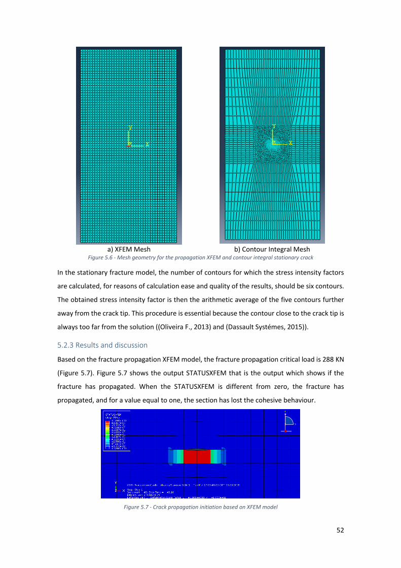
52
a) XFEM Mesh b) Contour Integral Mesh
Figure 5.6 - Mesh geometry for the propagation XFEM and contour integral stationary crack
In the stationary fracture model, the number of contours for which the stress intensity factors
are calculated, for reasons of calculation ease and quality of the results, should be six contours.
The obtained stress intensity factor is then the arithmetic average of the five contours further
away from the crack tip. This procedure is essential because the contour close to the crack tip is
always too far from the solution ((Oliveira F., 2013) and (Dassault Systémes, 2015)).
5.2.3 Results and discussion
Based on the fracture propagation XFEM model, the fracture propagation critical load is 288 KN
(Figure 5.7). Figure 5.7 shows the output STATUSXFEM that is the output which shows if the
fracture has propagated. When the STATUSXFEM is different from zero, the fracture has
propagated, and for a value equal to one, the section has lost the cohesive behaviour.
Figure 5.7 - Crack propagation initiation based on XFEM model

53
Once the critical load 𝐹𝑐 is known, the critical stress intensity factor 𝐾𝐼𝐶 (or fracture toughness)
can be calculated using Equation 5.2:
𝐾𝐼𝐶 =288000
2 × 0,02√0,002𝜋 (1 −
0,002
2 × 0,02)(1 −
0,02
2 × 0,002)
−12⁄
= 0,5715 𝑀𝑃𝑎√𝑚 = 571,5 𝐾𝑃𝑎√𝑚
(5.4)
Based on Equation 5.3, the critical fracture energy is then:
𝐺𝐼𝐶 =
1 − 0,22
1,427 × 1010(0,5715 × 10⁶)2 = 21,97
𝑁
𝑚≈ 0,022
𝐾𝑁
𝑚
(5.5)
On the other hand, from the stationary fracture model output file, the values of the stress
intensity factors calculated for the various contours can obtained and these are shown in Figure
5.8.
Figure 5.8 - Contour stress intensity factors for F=288KN
The stress intensity factor is then the average of the values obtained on the specified contours,
ignoring the contour closest to the crack tip:
𝐾𝐼 =
422,3 + 506,2 + 578,0 + 641,8 + 699,0
5= 569,5 𝐾𝑃𝑎√𝑚
(5.6)
It is found that the difference between the numerical results and the theoretical solution is only
0.35%. The numerical models fully reproduce the test of the infinite plate with a central crack
under tension.
5.3 Numerical modelling of oriented perforations
The aim of this section is to simulate numerically, using the Abaqus 6.14, the laboratory
experiments described by Abass H. et al. (1994) in order to analyze the effect of oriented
perforations in drilling wells when using the technique of hydraulic fracturing. This study focuses
on phenomena such as the initiation and propagation of hydraulic fractures in vertical wells. As
noted previously, these experimental tests were previously simulated using the XFEM in
Medinas M. (2015). However in that study hydraulic fracturing was simulated as a mechanical
pressured applied on the walls of the borehole and it was found that the results were
significantly affected by the simplification introduced by the manner in which the load was being

54
applied. In the present study, fluid injection is explicitly considered and the tests are model by
means of fully couple hydro mechanic XFEM analyses.
5.3.1 Experimental setup and material parameters
Abass H. et al. (1994) describe a series of laboratory test on blocks of hydrostone (Gypsum
cement) in a water / hydrostone weight ratio of 32: 100, with dimensions 0.154 m x 0.154 m
0,254 m.
Figure 5.9 - Core sample geometry, wellbore and perforations (Abass H. et al, 1994)
The study focused on perforations at 180° phasing, having been studied the direction (θ) of 0°,
15°, 30°, 45°, 60°, 75° and 90° relative to the preferred fracture plane (PFP, that corresponds to
the maximum horizontal stress direction), as shown in Figure 5.10. A total of 10 perforations
were made on each block, 5 on each side. The perforations were 12.7 mm long with 3.429 mm
diameter.
a) b) perforation at PFP Figure 5.10-Perforations direction relative to the PFP b)
In all tests the fracturing fluid was a 90-weight gear oil with approximately 1180 cp viscosity,
with an injection rate of 3 × 10⁻⁵ 𝑚3/𝑚𝑖𝑛. It was assumed that the initial pore pressure 𝑃𝑝𝑖
present within the samples was is zero (Abass H. et al, 1994).
The samples were confined in a true triaxial apparatus under 20670 kPa vertical stress, 17240
kPa maximum horizontal stress and 9650 kPa minimum horizontal stress. True-triaxial loading is

55
typically applied through a series of rigid platens, flexible bladders and passive confinement (e.g.
steel casing) (Frash L. P. et al, 2014), as seen in figure 5.11.
In a typical true triaxial apparatus configuration loading is applied via one active hydraulic flat
jack per principal axis. Specimen faces that contact directly with the flat jack are usually referred
to as active faces while faces that are in contact with the frame where a reaction is mobilized
are referred to as passive faces (Figure 5.12). Though true triaxial tests can replicate the in-situ
conditions more accurately than conventional triaxial test, the test is hard to conduct due to the
difficulties in equipment utilization, difficulties in sample preparation and pore pressure
measurements during the test (Zoback M., 2007).
Figure 5.11 - Schematic of a true-triaxial hydraulic fracturing test system (Chen M. et al, 2010)
Figure 5.12 - Interior design of a true-triaxial apparatus (Frash L. P. et al, 2014)
The description above refers to typical characteristics of a true triaxial test. However Abass H.
et al, (1994) do not give specific information regarding the way loads were applied, the stiffness
of the equipment and materials used. It is known that in the work presented by Abass H. et al,
(1994) the equipment is not servo-controlled and the minimum horizontal stress was monitored
(and significant variation was recorded) during fracture propagation.

56
5.3.2 Material parameters
The physical and mechanical properties adopted in the numerical analysis are shown in Table
5.2.
Table 5.2 - Physical and mechanical properties of Abass H. et al. (1994) samples
Rock Sample Properties
Dimensions 0,1525 × 0,1524 × 0,254 𝑚 Wellbore radius 0,00747 𝑚 Elastic Modulus 1,714e7 KPa
Poisson ratio 0,228 Permeability 9,5 𝑚𝐷 Porosity 0,277 Fracture Toughness 2,5 𝑀𝑃𝑎√𝑚 Fracture energy 0,341 𝐾𝑁/𝑚 Fracturing fluid density 0,92𝜌𝑤 Fracturing Fluid viscosity 1180 𝑐𝑃
Friction coefficient 0,0001 Fluid Leak-off coefficient 1 × 10⁻¹⁴ 𝐾𝑃𝑎. 𝑠 Tensile strength (Brazilian Test determined) 5560 𝐾𝑃𝑎
Fracture toughness is not an intrinsic property of the material, but depends on the geometry of
the sample under study, as illustrated in section 5.2. Because one of the input parameters
required for the initialization of the numerical model (i.e. fracture energy) is function of fracture
toughness, a value for this quantity had to be adopted. In the absence of any information
regarding the value of fracture toughness for gypsum cement, the value used in Liu L. et al.
(2014) equal to 2,5 𝑀𝑃𝑎√𝑚 was adopted, which is in the range of typical fracture toughness
values for rocks (see section 3.3.6).
In Abass H. et al. (1994) no consideration is made regarding the friction on the fracture surface.
To ensure the model representativeness, friction is considered in the fracture surface contact
area to account for the effect of frictional energy dissipation at fracture level and its influence
in fracture reorientation and propagation, and a low value of friction coefficient is initially
employed. The influence of this parameter is further investigated in Chapter 6.
According to Abass H. et al. (1994) experiences were performed with a zero initial pore pressure
and that was prescribed in the numerical analysis. In agreement, the initial pore saturation was
also set equal to zero.
The consideration of a non-zero fluid leak-off coefficient guarantees the introduction of some
important aspects of the fracturing fluid flow, since this parameter is required to compute the
normal component of the fluid velocity within the fracture (Zielonka M. G. et al, 2014). No
indication is given in Abass H. et al. (1994) regarding this parameter, and thus a low value equal

57
to 1 × 10⁻¹⁴ 𝐾𝑃𝑎. 𝑠 is initially adopted. The influence of this parameter is subsequently
analysed in Chapter 6.
Abaqus XFEM software assumes the end of cohesive behavior when 𝐺 > 𝐺𝑓 , where 𝐺𝑓 is the
critical fracture energy. The value of 𝐺𝑓 corresponds to the integral of the stress-displacement
diagram, as shown in Figure 5.13.
Figure 5.13 - Energy-based damage evolution for linear softening (Dassault Systémes, 2015)
Where 𝑢𝑓𝑝𝑙
is the displacement to reach the end of cohesive behavior and 𝜎𝑦0 is the tensile
strength of the rock.
Given the loading conditions applied in the analysis presented herein, the MAXPS (Maximum
principal stress) failure criterion is adopted. This is mathematically described as:
𝑀𝐴𝑋𝑃𝑆 = 𝑀𝑎𝑥𝑖𝑚𝑢𝑚 𝑝𝑟𝑖𝑛𝑐𝑖𝑝𝑎𝑙 𝑠𝑡𝑟𝑒𝑠𝑠 = 𝑓 = {
⟨𝜎𝑚𝑎𝑥⟩
𝜎𝑚𝑎𝑥0 }
(5.7)
Where 𝜎𝑚𝑎𝑥 is the stress at a specific point, 𝜎𝑚𝑎𝑥0 is the tensile strength of the rock and the
symbol ⟨ ⟩ is the Macaulay bracket that is used to ensure that a compressive stress state does
not initiate damage, and a fracture is initiated or the length of an existing fracture is extended
by tensile stresses, when the fracture criterion, 𝑓, reaches the value 1.0 within a specified
tolerance:
1,0 < 𝑓 < 1,0 + 𝑓𝑡𝑜𝑙
(5.8)
Where 𝑓𝑡𝑜𝑙 is the tolerance for the initiation criterion. As the simulation of fracture propagation
can be relatively instable, most authors (Dassault Systémes, 2015) propose a value of 0,2 for the
tolerance, and that is the value adopted in the analysis shown here.
The rock strength degradation/damage evolution (i.e. softening behavior) begins when the
failure criterion is verified and progresses linearly until total damage and loss of the section
cohesive behavior is reached.

58
The hydrostone was modelled as a linear elastic material with a damage law for traction
separation. The MAXPS (Maximum principal stress) failure criterion is considered, which is given
by Equation 5.7. In the absence of further information, it was considered an energy type damage
evolution law, using a power law function with power equal to 1,0 and fracture energy equal to
0.341 kN/m.
5.3.3 Model geometry and finite element mesh
This set of analyses aims to simulate in an adequate manner the experiments described in the
previous section, in particular the initiation and propagation mechanism of fractures. The
experiments are modelled by means of a series of coupled hydro-mechanic two-dimensional
plane strain analyses. This simplification (of reducing a 3D problem into a simpler 2D problem)
greatly simplifies the numerical procedure and reduces computing costs and time. Assuming 2D
plane strain conditions means that displacements perpendicular to the analysis plane (in this
case the vertical or z direction) are zero; however the stresses in the z direction are non-zero.
The plane strain assumption is a reasonable approximation when running simplified studies of
hydraulic fracturing. However it is found to lead to an overestimation of fracture width, due to
the restrictive effect of the tips only in the xy direction, as it cannot account for similar restriction
in the z direction (Valkó P. et Economides M. J., 1995). Given that in this study fracture width is
a secondary output, the assumption is made.
To avoid any kind of scale effects the geometry adopted in the numerical analysis corresponds,
as much as possible, to that of the laboratory experiments.
Figure 5.14 - Model geometry and partition faces
Figure 5.14 shows the model geometry and the domain partition. These partitions were
introduced to optimize the mesh and the numerical calculation process, by separating the more
complex areas, such as the wellbore, of the remaining areas under study. Abaqus software

59
allows the use of a different meshing technique for each partition. Therefore to minimize the
influence of the mesh, structured meshes are used in most of the analysis domain (with different
coarseness depending on the expected stress/strain changes) and in the wellbore zone is used
a free mesh to overcome the complex geometry of the area (Figure 5.15).
The analyses described in this thesis are hydro-mechanic coupled analyses and thus pore
pressure/ displacement finite elements are used.
Sensitivity analyses were performed to assess the influence of the mesh coarseness and
configuration on the analysis results. Three structured meshed were considered: extra-fine, fine
and coarse, as shown in figure 5.15. The number of nodes and elements in each mesh is
summarized in Table 5.3.
Extra-fine Fine Coarse
Figure 5.15 - Different Mesh configuration for XFEM oriented perforations study
Table 5.3 - 2D different mesh properties for XFEM oriented perforations study
Extra-fine Fine Coarse
Elements Linear Quadrilateral Linear Quad. Linear Quad.
type CPE4P CPE4P CPE4P
Number of nodes 13605 4184 1808
Number of elements 13345 4036 1704
When analyzing the results obtained with the 3 meshes, it appears that, despite predicting
reasonably well fracture reorientation, as a result of the large average element dimension, the
coarse mesh gives breakdown pressures for perforations directions above 30° that are not
consistent with Abass H. et al. (1994) experimental results.
The fine mesh provides adequate simulation of fracture initiation and propagation for most
cases; However, due to the high mesh dependency of the XFEM, the study of 60° and 90°
directions, is made using the extra-fine mesh, despite the significant increase in simulation time
and memory consumption.

60
5.3.4 Boundary condition and loading procedure
Since in Abass H. et al. (1994) there is no specific information regarding the apparatus used in
the experiments, the definition of loading and boundary conditions to be adopted in the
analyses becomes more difficult, and a set of simplifications needs to be introduced.
Abass H. et al. (1994) states that the tests were performed in non-servo controlled conditions.
In that case, and due to the fact that the stiffness of the testing equipment may be of the same
order of magnitude of the sample stiffness, the stresses applied to the sample facets are not
maintained constant, and Abass et al. (1994) report that significant changes in the minimum
horizontal stress were recorded. Since it is not given any information regarding the true triaxial
used, it is not possible to ascertain what is the stiffness of the equipment, and it is only known
that the passive and active platen are often of concrete (E = 30 GPa) and steel (E = 200 GPa),
respectively.
Following the study of Medinas M. (2015) various options for the displacements boundary
conditions were considered. The adopted boundary conditions are shown in Figure 5.16 and
both horizontal and vertical displacements were restrained along the samples outer boundaries.
Because in the analyses describe herein the fluid is modelled explicitly, hydraulic fracturing
operations, i.e. fluid injection, do not affect the stresses at the boundaries and the reactions
developed at the boundaries are very small and do not affect the analysis results.
Figure 5.16 - Displacement boundary conditions for the oriented perforations experience
As noted fluid injection is simulated explicitly and it is considered that the fluid injection rate
increases linearly during the first minute, up to 5 x 10 -7 m3/s and then remains constant
throughout the fracturing operation (Figure 5.17).
𝜎𝐻 = 17,24 𝑀𝑃𝑎
𝜎ℎ = 9,65 𝑀𝑃𝑎

61
Figure 5.17 - Fluid Injection amplitude through time
The use of an increasing injection flow in the first minute aims to increase the simulation stability
and avoid excessive and instantaneous pressure increments that could cause rock failure in
conditions different from those expected.
During the injection and fracturing process, the typical fracture pressure profile is similar to that
shown in Figure 5.18; the pressure increases until it reaches a peak that corresponds to the
breakdown pressure, after which there is a pressure relief in the fracture as a result of its
propagation until eventually it stabilizes (extension pressure) remaining constant until the end
of the injection process (shut-in). The remaining stages correspond to the closure of the fracture
in the long term as a result of overburden stresses, leading to screen outs, possibly only
prevented with a re-injection operation (Soliman M. Y. et Boonen P., 2000).
Figure 5.18- Typical fracture pressure profile during and post-injection (Soliman M. Y. et Boonen P., 2000)
From a real point of view, the injection causes the application of a pressure 𝑃𝑤 on all the exposed
surface of the wellbore. However, one of the XFEM limitations is the fact that flow injection
occurs at the fracture level, through the use of phantom nodes concept.
Comparing with the analytical models presented in section 3.4.3, the assumption that the fluid
is injected at fracture level is valid since the leak-off into the surrounding fluid is null or
0
0,2
0,4
0,6
0,8
1
1,2
0 1 2 3
Flu
id in
ject
ion
rat
e
Time (min)
Injection Amplitude
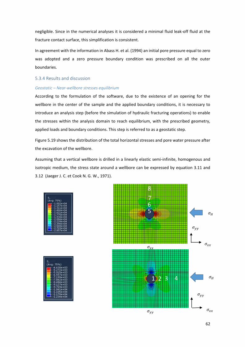
62
negligible. Since in the numerical analyses it is considered a minimal fluid leak-off fluid at the
fracture contact surface, this simplification is consistent.
In agreement with the information in Abass H. et al. (1994) an initial pore pressure equal to zero
was adopted and a zero pressure boundary condition was prescribed on all the outer
boundaries.
5.3.4 Results and discussion
Geostatic – Near-wellbore stresses equilibrium
According to the formulation of the software, due to the existence of an opening for the
wellbore in the center of the sample and the applied boundary conditions, it is necessary to
introduce an analysis step (before the simulation of hydraulic fracturing operations) to enable
the stresses within the analysis domain to reach equilibrium, with the prescribed geometry,
applied loads and boundary conditions. This step is referred to as a geostatic step.
Figure 5.19 shows the distribution of the total horizontal stresses and pore water pressure after
the excavation of the wellbore.
Assuming that a vertical wellbore is drilled in a linearly elastic semi-infinite, homogenous and
isotropic medium, the stress state around a wellbore can be expressed by equation 3.11 and
3.12 (Jaeger J. C. et Cook N. G. W., 1971).
𝜎𝑥𝑥
𝜎𝑦𝑦
5 6 7
8
1 2 3 4
𝜎𝐻
𝜎𝐻
𝜎𝑥𝑥
𝜎𝑦𝑦
𝜎𝑥𝑥
𝜎𝑦𝑦

63
Pore pressure
Figure 5.19 - Stress initialization due to wellbore excavation
When analysing Figure 5.19 is important to bear in mind that Abaqus convention is that positive
stresses correspond to tension and negative to compression, but the opposite applies to pore
pressure, such that negative pore pressures correspond to suctions. Despite the fact that at the
start of the analysis a zero pore pressure and zero saturation has been specified to all the
analysis domain, at the start of the geostatic step the software assumes 100% saturation. Given
that a small time step has been assigned to the geostatic step and the sample has a very small
permeability, the analysis predict an undrained response to the formation of the wellbore and
negative pore pressures (suctions) are predicted. The fluid injection is modelled immediately
after this geostatic step. It is acknowledge that stress conditions at the start of the fluid injection
predicted by the numerical analysis differ significantly from those existing in the laboratory tests
carried out by Abass et al. (1994).
Table 5.4 compares the value of the total tangential stress obtained in the numerical analyses
at the end of the geostatic step at a set of points (see figure 5.19), with the values obtained
through the application of Equation 3.12.
Table 5.4 - Comparison between measured initial tangential stresses between analytical and numerical solutions
Point 𝝈𝒏𝒖𝒎𝒆𝒓𝒊𝒄𝒂𝒍 𝝈𝒂𝒏𝒂𝒍𝒊𝒕𝒊𝒄𝒂𝒍 error(%)
1 -4,63 -11,71 60,5
2 -7,79 -13,62 42,8
3 -8,864 -12,3 28,0
4 -9,46 -10,4 9,0
5 -28,57 -42,07 32,1
6 -23,45 -29,4 20,2
7 -18,03 -19,89 9,4
8 -17,56 -17,8 1,3
It is found that the difference between the tangential stresses obtained in the numerical
analyses and those given by equation 4.12, reduces with the distance to the wellbore, presenting
an average error of 25,4% for this set of points. However some studies (Tie Y. et al, 2011) have
found that the analytical expression can lead to errors on the order of 25% when these are
applied to laboratory test samples with non-zero pore pressures. Another reason for the
𝜎𝐻

64
difference may be related with the influence area of the analytical equation, usually defined for
distances 2-3 times de wellbore radius (Sepehri J., 2014).
It appears that towards the preferred fracture plane (Points 1 and 2) the tangential stresses near
the wellbore are underestimated, as well as in the direction of 𝜎ℎ (Points 5 and 6).
Figure 5.20 shows the distribution of the pore pressure, after reequilibrium of the pore
pressures with the beginning of the fluid injection, showing that these stabilize at values around
8-10 MPa. Notice this equilibrium condition is independent of the geostatic step.
Figure 5.20 - Pore pressure distribution in the sample with the start of fluid injection
Breakdown pressure without perforation
The XFEM functionality enables the simulation of fracture initiation and propagation without
having to initially set its location. For the analysis without perforation, fracture initiated in the
direction of the maximum horizontal stress (i.e. the PFP) associated with an injected flow at the
element edge of 2,5𝑒−7 𝑚3/𝑠 and a breakdown pressure is obtained from the output PORPRES
and equal to 13,58 MPa. Theoretically that value should correspond to:
𝑃𝐵𝑘 = 𝜎′00 + 𝜎𝑇
(5.9)
Where 𝑃𝐵𝑘 is the breakdown pressure, 𝜎′00 is the effective tangential stress in the near-wellbore
expected fracture location and 𝜎𝑇 is the rock tensile strength.
Computing the values using the various output available, the following value is obtained:
𝑃𝐵𝑘 = 7,033 + 5,560 = 12,593 𝑀𝑝𝑎
(5.10)
The value 7,033 MPa is a tangential stress and was obtained from the numerical analysis at the
rock breakdown instant. It is thought that this difference of about 8% is related to the friction
effect on the fracture contact surface, as well as some difficulties in the numerical calculation of
the stresses around the fracture tip. According to Equation 5.10 the breakdown pressure
depends only of the tangential stresses at the fracture tip and the tensile strength of the
material.
65
Assuming the validity of equations 3.11 and 3.12 to describe the effective stresses around the
wellbore region, and invoking the material tensile failure criteria, the breakdown pressure is
then:
𝑃𝐵𝑘 = 3𝜎ℎ − 𝜎𝐻 − 𝑃𝑃 + 𝜎𝑇
(5.11)
Where 𝜎ℎis the minimum horizontal stress, 𝜎𝐻 is the maximum horizontal stress and 𝑃𝑝 is the
pore pressure in that location. Based on the integration of the numerical (pore pressure) and
theoretical values (stresses and tensile strength), the following expression is achieved:
𝑃𝐵𝑘 = 3 × 9,65 − 17,24 − (−1,7) + 5,56 = 18,97 𝑀𝑝𝑎
(5.12)
A 28,4% difference in relation to the value obtained in the numerical analysis is obtained. This
difference may be related to the re-equlibrium of the near-wellbore stress made on geostatic
step, since it was found that in the direction of the PFP, the stress values were underestimated.
It is verified that in this situation the injected flow rate to cause tensile failure of the sample
without perforation is 3187% the flow rate required to cause the failure when considering the
existence of a perforation in the same direction. This is extremely important when designing an
operation to minimize costs and ensure the project feasibility.
Breakdown pressure with oriented perforations
The breakdown pressure is the pressure required to cause the tensile failure of the rock at the
perforation tip. The breakdown pressure was calculated for the simulated perforations in the
angles θ = 0°, 15°, 30°, 45°, 60°, 75° and 90°, as seen in table 5.5.
Table 5.5 - Breakdown pressure for direction 0-90° for studied model
Breakdown pressure (MPa)
Direction
0° 12,36
15° 15,85
30° 20,09
45° 24,77
60° 25,8
75° 30,44
90° 32,18
As expected, there is an increase in the breakdown pressure as θ increases, since for higher θ,
near-wellbore tangential stresses are greater. It is also observed a slight reduction in breakdown
pressure in the direction 0° compared with the situation without initial perforation.
The results obtained for the breakdown pressure are compared with the results obtained in
laboratory (Abass H. et al, 1994), as seen in figure 5.21.

66
In directions lower than 45°, as result of the initial stress equilibrium, the model underestimates
the breakdown pressure values, and in the direction 45° there is a perfect match between
laboratory and numerical values which remain reasonably adjusted for the remaining directions.
Notice that for directions 45-90º the average error between the obtained values is 7% and the
breakdown pressure profiles are approximately parallel.
Figure 5.21 - Breakdown pressure comparison between (Abass, 1994) and the numerical simulation
Given that fracture initiation is mainly controlled by the tangential stresses in the crack tip region
(Economides M. J. et al, 2000), to explain the differences in breakdown pressure shown in Figure
5.21, the evolution of the tangential stress with the fluid injection is analysed.
Figure 5.22 shows the tangential stresses at the crack tip at the end of the geostatic step
following the stress re-equilibrium due to excavation of the wellbore and at the time of fracture
initiation.
Figure 5.22 - Tangential stresses in the initial geostatic equilibrium and through the tensile failure in the crack tip
The difference between these two data sets should provide an estimate of the changes in
tangential stresses at the crack tip caused by fluid injection. This effect is estimated at about 4
MPa for all perforation direction, except for 0° and 15°, where it is much smaller.
10
15
20
25
30
35
40
0 15 30 45 60 75 90
Bre
akd
ow
n p
ress
ure
(M
Pa)
Perforation Angle (θ)
(Abass,1994)
Numerical Results
0
5
10
15
20
25
30
0 15 30 45 60 75 90
Tan
gen
tial
Str
ess
(MP
a)
Perforation Angle (θ)
Initial Tangential Stress
Breakdown pressure tangential stress

67
Values of tangential stresses at perforation tip at the moment of fracture initiation occuring in
the laboratory samples are estimated, rewriting Equation 5.9 as:
𝜎′00 = 𝑃𝐵𝑘 − 𝜎𝑇
(5.13)
Figure 5.23 compared the values of tangential stresses at the crack tip obtained by application
of Equation 5.13 to the laboratory testing data with the numerical simulation results.
Figure 5.23 - Tangential stresses in crack tip for numerical and laboratorial results
There is still a difference between the Abass et al. (1994) experiments and the simulations
results. This difference, whose cause is not known, may be related to the friction coefficients
and leak-off coefficients used in the model.
Fracture reorientation
Fracture tends to propagate in a plane of least resistance, which is usually called preferred
fracture plane (PFP) and is perpendicular to the minimum horizontal stress. If the perforation
orientation is out of the direction of PFP, induced fracture may initiate along the perforation and
as it propagates away from the near wellbore toward the unaltered in-situ state of stress, will
reorient itself to be perpendicular to the minimum horizontal stress.
A visual comparison between Abass H. et al. (1994) results and the numerical simulations is
shown in Figures 5.24.
0
5
10
15
20
25
30
35
0 15 30 45 60 75 90
Tan
gen
tial
Str
ess
(MP
a)
Perforation Angle (θ)
(Abass,1994) tangential stresses
Breakdown pressure tangential stress

68
15 30
45 60
75 90
Figure 5.24 - Comparison of model simulation results with experimental results
Some authors state that the direction of propagation (θ) of fracture depends on the SIF loading
mode I and II (Zhang G. et Chen M., 2009). However that cannot be confirmed because, as noted
𝜎𝐻
𝜎𝐻
𝜎𝐻

69
in section 5.2, Abaqus only allows the examination of stress intensity factors when simulating
stationary fractures.
The analysis can be made based on the stress anisotropy, with the fracture to reorient to the
direction of greatest principal stress (perpendicular to the direction of least principal stress), if
the stress anisotropy is enough to ensure fracture reorientation.
To analyse in a quantitative manner fracture reorientation, the fracture was digitalized using
software Data GetGraph Digitalizer, and the data treated to obtain the variation of the fracture
direction along its length (Figure 5.25).
15° 30°
45° 60°
75° 90° Figure 5.25 - Fracture reorientation for all perforation directions
-100
102030405060708090
0 2 4 6 8 10
An
gle(°)
Distance from perforation tip (mm)
-100
102030405060708090
0 1 2 3 4 5 6 7 8 9 10 11 12 13
An
gle(°)
Distance from the perforation tip (mm)
-20-10
0102030405060708090
0 2 4 6 8 10 12
An
gle(°)
Distance from the perforation tip (mm)
-20-10
0102030405060708090
0 5 10 15 20 25
An
gle(°)
Distance from the perforation tip (mm)
0102030405060708090
0 5 10 15 20 25 30
An
gle(°)
Distance from the perforation tip (mm)
0102030405060708090
20 40 60 80
An
gle(°)
Distance from the perforation tip (mm)

70
In the directions 15° to 45° there is the so-called pinch effect, which makes the fracture initial
reorientation to be negative. In the other directions this effect is not felt, as studied in more
detail later in this chapter.
Another way to analyze fracture reorientation is using the concept of reorientation radius, which
is the distance from the wellbore to the point where fracture is completely aligned with PFP, as
shown graphically in Figure 5.26.
Figure 5.26 - Schematic representation of reorientation radius (Chen M. et al, 2010)
Table 5.6 shows the reorientation radius for different perforation angles. This distance should
be considered with caution as a result of the pinch effect which occurs in directions 15°- 45°.
Table 5.6 - Reorientation radius for different perforation angle
Angle Reorientation radius
15 2,62𝑟𝑤
30 3,07𝑟𝑤
45 2,86𝑟𝑤
60 3,28𝑟𝑤
75 4,13𝑟𝑤
90 6,27𝑟𝑤
Based on the results presented in the Figure 5.24 and Table 5.6 it appears that fracture
reorientation towards the PFP is achieved in all directions. The larger the perforation angle, the
greater the reorientation angle and thus the distance required for the fracture to re-orientate.
The slight reduction in the reorientation radius from perforation angle 30° to 45° is related with
pressure peaks at the fracture tip immediately after fracture initiation, which generates an
instantaneous stress anisotropy, giving rise to a larger reorientation than expected. According
to Abass H. et al. (1994), during injection is verified the existence of peak pressures at the
fracture tip, which goes with the numerical results. However this effect may be due to the
instability of XFEM associated with mesh dependency in directions near 45°.

71
In the directions 15° to 45° there is the so-called pinch effect, which makes fracture
reorientation analysis more difficult. According to Zhang X. et al. (2011) and Cherny S. et al.
(2009) the pinch effect is a consequence of the adopted friction coefficient, which is an input
parameter of the analysis. This effect can cause a slight increase in the reorientation radius and
difficulties related with the fluid injection and subsequent loss of productive capacity as a
consequence of the fracture width reduction. This effect will be studied later in this chapter in
more detail.
As said before, fracture reorientation seems to be dictated by the stress anisotropy at the crack
tip. The tendency for the fracture to propagate toward the initial perforation direction increases
as the anisotropy ratio tends to 1 (Solyman M. Y. et Boonen P., 1999).
Therefore the evolution of the anisotropy at the crack tip while fracture propagates and re-
orientates has been analysed, and is shown in Figure 5.27 and table 5.7, for perforation angle
equal to 90°. Notice that herein the anisotropy ratio is the ratio between the vertical (yy) stresses
and the horizontal (xx) stresses at the fracture tip.
Figure 5.27 - Stress Anisotropy ratios for different moments in the crack propagation for 90° perforation angle Table 5.7 - Stress Anisotropy ratios for different moments in the crack propagation (at the element level) for 90°
perforation angle
Points (1) (2) (3) (4) (5) (6) (7) (8)
Anisotropy ratio (𝝈𝒚𝒚/𝝈𝒙𝒙)
1,31 1,49 1,69 2,89 1,97 2,04 1,73 1,88
Initially fracture reorientation to the PFP does not occur, since the stress anisotropy ratios are
just above 1, with a tendency to grow. After (4), where the stress anisotropy ratio is equal to
2,89 there is a clear shift in fracture orientation and then to a lesser degree following (5).
With the initiation of fracture reorientation there is a tendency for the fracture to maintain the
previous propagation direction if there is no change in anisotropy. A further increase in the ratio
(6) , allows the reorientation to the PFP direction in which eventually remain, since the
subsequent local anisotropy ratios are not generating any reorientation in the fracture.
(5)
(1)
(6) (7)
(3)
(8)
(2)
(4) 𝜎𝐻

72
Abass H. et al. (1994) note that, in practice, the use of perforation angles above 30°- 45° is very
complicated, as result of tortuosity introduced by the reorientation, which reduces the
communication between the fluids and the fracture, with possible fracture width reductions and
followed by fluids screen out. This effect is studied below.
Fracture Width
Fracture reorientation can cause tortuosity that can lead to reductions in fracture width for a
certain applied pressure. The loss of communication between the perforation and fracture is
defined based on a geometry factor defined as (Abass H. et al, 1994):
𝐺𝐹 =
𝐴𝑐𝑜𝑚
𝐴𝑝𝑒𝑟
(5.14)
Where 𝐴𝑐𝑜𝑚 is the communication area between the fracture and the perforation tunnel and
𝐴𝑝𝑒𝑟 is the perforation cross-sectional area.
The fracture width (𝑊𝑓) is calculated as:
𝑊𝑓 =
2𝐷
𝐸(𝑃𝑓 − 𝜎ℎ)
(5.15)
Where D is half-length of the sample in a principal direction and E is the Young’s modulus.
Differentiating Equation 5.15 with respect to time:
𝑊𝑓
𝑑𝑡=
2𝐷
𝐸
𝑑
𝑑𝑡(𝑃𝑓 − 𝜎ℎ)
(5.16)
The width function is expressed as:
𝑊𝑖𝑑𝑡ℎ 𝑓𝑢𝑛𝑐𝑡𝑖𝑜𝑛 =
𝑊𝑓
𝑑𝑡
𝐸
2𝐷=
𝑑
𝑑𝑡(𝑃𝑓 − 𝜎ℎ)
(5.17)
Analyzing the average opening of the fracture at the crack tip level (with the output
PFOPEMXFEM) for the various directions for a range of different accumulated injected flows, is
possible to verify that the fracture opening is similar for a injected flow of 3,75 × 10⁻⁶ 𝑚3, as
can be seen in table 5.8.
Table 5.8 - Fracture opening (mm) for different perforation direction to different injected flows
Direction 𝑰𝒏𝒋𝒆𝒄𝒕𝒆𝒅 𝒇𝒍𝒐𝒘 = 𝟑, 𝟕𝟓 × 𝟏𝟎−𝟔 𝒎𝟑
𝑰𝒏𝒋𝒆𝒄𝒕𝒆𝒅 𝒇𝒍𝒐𝒘 = 𝟓 × 𝟏𝟎−𝟔 𝒎𝟑
0 2,0395 2,0395
15 2,0340 2,0330
30 2,0359 2,0320
45 2,0350 2,0314
60 2,0437 2,0335
75 2,0417 2,0332
90 2,0362 2,0289
It is found that this initial opening to directions different of zero (PFP) is rapidly reduced to lower
values of injected flow. Once this is the magnitude of the injected flow for fracture propagation,
this effect shows the effect of the tortuosity for all directions less the non deviated perforation.

73
However, this effect should be more accentuated with the perforation direction deviation
increase with the PFP. The openings in the directions 60 °and 75° for the two analyses stages
considered in Table 5.8, do not comply with the stated above. This can be related to pressure
peaks due to numerical calculation difficulties, since the data does not follow the trend observed
at smaller perforation angles.
According to Abass H. et al. (1994), it appears that for directions less than 45, there is a clear
increase in fracture width with fluids injection. However, Abass H. et al. (1994) found that for
directions above 45°, as fracture propagation progresses the fracture width function tends to
zero, becoming even negative to 75-90° directions, which indicates fracture width reduction and
possible consequent the fluid screen-out. This effect is resultant of fracture tortuosity.
Table 5.9 shows the values of the fluid pressure in fracture and 𝜎ℎ, at 5 instances of the analysis
procedure when admitting a perforation angle equal to 90°, in order to assess their effect in the
fracture opening. Figure 5.28 shows the propagation of the fracture at the same instances.
Table 5.9 - Fracture opening rate (Width function) verification to direction 90°
Injected Flow - 10s
Injected Flow - 20s
Injected Flow - 23,99
Injected Flow - 31s
Injected Flow - 60s
𝑷𝒇 (MPa) 32,06 23,10 14,43 4,74 7,26
𝝈𝒉 (MPa) 18,57 16,88 11,71 9,21 6,42
𝑷𝒇 − 𝝈𝒉
(MPa)
13,49 6,22 2,72 -4,47 0,84
Fracture opening
2 2,0288 2,0288 2,0210 2,0943
10s 20s 23,99s
31s 60s
Figure 5.28 - Fracture propagation with fluid injection

74
It is found that initially and as a result of the existent stress anisotropy, the fracture propagates
in the vertical direction, and an increase in the fracture opening is found. Since the tangential
stresses in the surrounding of the fracture are very high, the extension of the fracture is small.
With the continued fluid injection, the fracture propagates and it reorientates towards the PFP.
It is found, at this stage, a reduction of fracture opening, with the fracture function width to take
even negative values, which can generate screenout effects. This decrease in fracture pressure
may be related to the tortuosity and loss of communication between the perforation and the
fracture, which hinders the access of the fluid to the crack tip zone (fluid lag effect).
Nevertheless it appears that with a major increase in the injected flow, there is a significant
increase in fracture opening, either due to a reduction in the tortuosity effect or as a result of
the reduction in tangential stresses and loss of fracture cohesive behaviour. The reduced
permeability of the sample is one of the decisive factors that contribute to the increase in
fracture width, since the fluids are located in the fracture and the amount of fluid lost (fluid leak-
off) into the surrounding area is minor.
Fracture Pressure profile
Figure 5.29 shows the evolution of the fluid pressure in the fracture with time, obtained in the
numerical simulations for a perforation angle equal to 0°.
Figure 5.29 - Fracture Pressure profile for perforation near-crack tip for direction 0
Comparing Figure 5.29 with Figure 5.18 (that shows a typical pressure profile in the fracture
during HF operations) it is found that the various stages are represented in the numerical curve.
Table 5.10 shows the average fracture pressure at equilibrium (i.e. the extension pressure) for
the various perforation angles, obtained from an Abaqus output file
Table 5.10 - Equilibrium fracture pressure for different perforation direction after reorientation to the PFP
Direction Without perforation
0 15 30 45 60 75 90
Equilibrium pressure (MPa)
5,09 4,73 5,31 5,46 6,08 6,41 6,43 7,30

75
It is found an increase in the equilibrium pressure for higher directions. This can be explained by
the increase of the tangential stresses, as θ increases. It is found that the equilibrium pressure
for the situation without initial perforation is similar to the direction 0° with perforation.
It should be noted that as indicated in Abass H. et al. (1994), some peak pressures are felt in the
fracture during the injection phase. These can explain the pressure increments before fracture
reorientation. In the numerical simulations the pressure peaks may as well result of numerical
calculation difficulties instead.
The XFEM functionality is heavily dependent on mesh and the location of the fracture tip. The
adopted procedures aimed to ensure that the results presented herein where not affected by
these aspects or numerical instabilities. However their influence cannot be ruled out.

76
6. Validation - Parametric study
The studies described in the previous chapter, i.e., the simulation of a fracture toughness
determination test and the laboratory tests described by Abass H. et al. (1994) on induced
fractures using oriented perforations, showed that Abaqus XFEM software is able to analyze
with confidence the mechanical behaviour of rocks, fracture initiation and propagation by fluid
injection.
Based on the model set up used for the simulation of the laboratory tests described by Abass et
al. (1994), in this chapter, it is presented a numerical study on the effect of a series of parameters
on the outcome of hydraulic fracturing operations, in particular the breakdown pressure and
fracture re-orientation. The parameters considered in this study are porosity, permeability,
friction, anisotropy, fluid viscosity, fluid leak-off, flow rate, perforation phasing and phasing
miss-alignment. For simplicity it will only be considered perforations oriented at 0°, 45° and 90°
with the PFP.
6.1 Porosity
Porosity is one a rock physical properties and different porosities were studied: 13,25%; 6,625%
and 3,3125% in addition to the base case of 27,7%. This effect is not documented in the
literature.
It was found that the porosity does not affect the fracture initiation and propagation, since no
changes were identified in the breakdown pressure, fracture reorientation profile or fracture
width.
6.2 Permeability
Permeability is a rock physical property which affects the fluid displacement velocity within the
sample. Different permeabilities were used: 50mD, 30 mD, 5mD, 2,5 mD and 0,5mD, in addition
to the base case of 9,5 mD permeability.
The breakdown pressure for the different permeability values and perforation directions was
calculated, and is presented in Figure 6.1.
It is possible to verify that with an increase in permeability, the breakdown pressure also
increases. The increase in permeability increases the capacity of the fluid to move within the
rock pore space, which increases the effective stresses around the perforation, and thus the
tangential stresses.

77
Figure 6.1 - Breakdown pressure for different directions and different permeabilities
The breakdown pressure variation with the permeability for the different directions follows the
same evolution path, which indicates that the effect of the perforation direction has a low
impact in the variation of the breakdown pressure when changing the rock permeability.
While the permeability increases, the injected flow that induces the breakdown pressure also
increases for the different directions, as seen in figure 6.2. This was anticipated, once that for
higher permeability it is easier for the fluid to move through the rock mass and it is necessary
sufficient fluid material to sustain the fracture opening and avoid the screen out effect. For
higher permeabilities the injected flow is similar, and follow the same trend of the breakdown
pressure for high permeabilities (see Figure 6.1 and 6.2).
Figure 6.2 - Evolution of the injected flow with permeability for different perforation directions
The fracture reorientation path is also affected by the adopted permeability, as can be seen in
figure 6.3 and figure 6.4.
0
5
10
15
20
25
30
35
40
45
50
0 5 10 15 20 25 30 35 40 45 50
Bre
akd
ow
n P
ress
ure
(M
Pa)
Permeability (mD)
Direction 0
Direction 45
Direction 90
0,E+00
5,E-07
1,E-06
2,E-06
2,E-06
3,E-06
3,E-06
0 10 20 30 40 50
Inje
cted
flo
w (
m3 )
Permeability (mD)
Direction 0
Direction 45
Direction 90

78
50 mD 9,5 mD
5 mD 0,5 mD
Figure 6.3 - Fracture propagation for different permeabilities to a perforation in direction 45
Figure 6.3 suggests that the pinch effect reduces with increasing permeability increases, due to
the stress changes introduced by the fluid injection.
50 9,5
5 0,5
Figure 6.4 - Fracture propagation for different permeabilities to a perforation in direction 90
Although there is a tendency of the complete reorientation to the PFP to happen for bigger
distances (i.e higher reorientation radius), the perforation in direction 90° reorientation to the
PFP happens earlier (in terms of Cartesian distance) as lower the permeability.
The flow injected to achieve complete reorientation of the fracture to the PFP is found to
increase with permeability, as seen in figure 6.5.
𝜎𝐻
𝜎𝐻
𝜎𝐻
𝜎𝐻

79
Figure 6.5 - Injected flow for the complete reorientation to the PFP of 90° perforations
The reduction in fluid injection to achieve complete fracture reorientation for lower
permeabilities has consequences on the evolution of fracture width.
For lower permeabilities, the fluid displacement (i.e. percolation) is lower to the surrounding
media and the fluid within the fracture is higher (due to less fluid loss) inducing greater fracture
openings that in a high permeability rock, increasing the productivity of the fracture and the
economic feasibility of the operation.
6.3 Friction coefficient
The fracture surface friction coefficient influences the fracture reorientation path, and the so-
called pinch effect is a direct consequence of the friction coefficient. More information regarding
the principles and effects of the friction coefficient in the fracture reorientation can be found in
the literature (Zhang X. et al, 2011). Different coefficients were used: 0,000001; 0,0001 (base
case); 0,01; 0,1.
This effect may be felt in all the perforation direction, however, due to the higher tangential
stresses in perforations 60° or more from the PFP, the effect of the friction coefficient becomes
residual when compared with the in-situ stress state (Zhang X. et al, 2011).
The direction of the model that shows more clearly the pinch effect is the direction 45°, for
which the influence of the fracture surface friction on the fracture propagation is shown in
Figure 6.6.
The pinch effect is noticed for friction coefficients lower than 0,1 (case d). Higher friction
coefficients were not studied because the software was providing numerically unstable and
having difficulties in reaching convergence.
0,0E+00
1,0E-06
2,0E-06
3,0E-06
4,0E-06
5,0E-06
6,0E-06
7,0E-06
8,0E-06
0 10 20 30 40 50
Inje
cted
flo
w (
m3 )
Permeability (mD)
Injected Flow
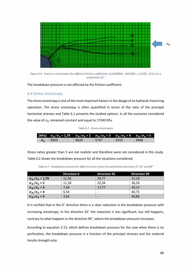
80
Figure 6.6 - Fracture reorientation for different friction coefficients: a) 0,000001 ; b)0,0001 ; c) 0,001 ; d) 0,1 to a
perforation 45°
The breakdown pressure is not affected by the friction coefficient.
6.4 Stress Anisotropy
The stress anisotropy is one of the most important factors in the design of an hydraulic fracturing
operation. The stress anisotropy is often quantified in terms of the ratio of the principal
horizontal stresses and Table 6.1 presents the studied options. In all the scenarios considered
the value of 𝜎𝐻 remained constant and equal to 17240 KPa.
Table 6.1 - Stress anisotropies
(KPa) 𝝈𝑯/𝝈𝒉 = 1,79 𝝈𝑯/𝝈𝒉 = 2 𝝈𝑯/𝝈𝒉 = 3 𝝈𝑯/𝝈𝒉 = 4 𝝈𝑯/𝝈𝒉 = 5
𝝈𝒉 9650 8620 5747 4310 3448
Stress ratios greater than 5 are not realistic and therefore were not considered in this study.
Table 6.2 shows the breakdown pressure for all the situations considered.
Table 6.2 - Breakdown pressure for different stress ration for perforation directions 0°, 45° and 90°
Direction 0 Direction 45 Direction 90
𝝈𝑯/𝝈𝒉 = 1,79 12,36 24,77 32,18
𝝈𝑯/𝝈𝒉 = 2 11,18 22,34 36,26
𝝈𝑯/𝝈𝒉 = 3 7,46 17,77 39,13
𝝈𝑯/𝝈𝒉 = 4 6,54 - 40,75
𝝈𝑯/𝝈𝒉 = 5 3,64 - 40,86
It is verified that in the 0° direction there is a clear reduction in the breakdown pressure with
increasing anisotropy. In the direction 45° the reduction is less significant, but still happens,
contrary to what happens in the direction 90°, where the breakdown pressure increases.
According to equation 3.13, which defines breakdown pressure for the case when there is no
perforation, the breakdown pressure is a function of the principal stresses and the material
tensile strength only.
a)
c) d)
b) 𝜎𝐻

81
For perforation direction 0°, a reduction in the breakdown pressure would be expected, because
𝜎ℎ controls the tangential stresses generated in the direction normal to the perforation
direction, and subsequently the reduction in the breakdown pressure.
Although, if this result is purely compared with the analytical expression (equation 3.13) , the
result is coherent, because the near-wellbore stress re-equilibrium for high stress anisotropy
requires even negative breakdown pressures for direction 0°, as seen in table 6.3. This negative
value means that the stresses generated in the near-wellbore region are tensile stresses.
Table 6.3 - Analytical breakdown pressure values for different stress ratios to direction 0° and 90° (without
perforation) – Based on equation 3.12
(MPa) 𝝈𝑯/𝝈𝒉 = 1,79 𝝈𝑯/𝝈𝒉 = 2 𝝈𝑯/𝝈𝒉 = 3 𝝈𝑯/𝝈𝒉 = 4
𝝈𝑯/𝝈𝒉 = 5
Direction 90 47,63 48,66 51,53 52,97 53,83
Direction 0 17,27 14,18 4,74 1,25 -1,34
For perforation direction 90°, is verified an increase in the breakdown pressure for higher stress
anisotropy ratios. This effect is also verified in the experiments of (Chen M. et al, 2010) and in
table 6.3 results. This effect is a consequence of the different stress re-equilibrium in the near-
wellbore region for different stress anisotropy ratios. A different stress state generate the higher
or lower tangential stresses at the perforation tip, and consequently different breakdown
pressures, even with a constant maximum principal stress.
In the direction 45° there is an intermediate change between the two cases explained; this is
because it is not a principal stress direction, resulting in an intermediate solution. Notice
however that for the three studied directions, the injected fluid at fracture initiation (at
breakdown pressure) decreases for higher stress anisotropy ratios, as can be seen in figure 6.7.
Figure 6.7 - Injected flow to cause the rock tensile failure for different directions and anisotropy ratios
The stress anisotropy has an effect in fracture reorientation, as seen in Figure 6.8 and 6.9.
5,E-07
1,E-06
2,E-06
2,E-06
3,E-06
3,E-06
1,5 2 2,5 3 3,5 4 4,5 5
Inje
cted
flo
wv
(m3)
Stress Anisotropy
Direction 0
Direction 45
Direction 90

82
Figure 6.8 - Fracture propagation for different stress ratio in direction 90°
Figure 6.9 - Fracture propagation for different stress ratio in direction 45°
The effect of the reorientation with the stress anisotropy is more apparent in the 90° direction
than in 45°. This occurs because the stress equilibrium in the proximity of the fracture in 90°
direction ensures the existence of significant reductions in normal stresses, allowing the fracture
to reorientate toward PFP, i.e. the fracture tip stress state for direction 90° is more influenced
than the direction 45°, once in this is not a principal direction
In direction 45°, a small increase in the pinch effect is felt at high anisotropy ratios. Notice that
for higher stress anisotropies the simulations for the 45° direction perforations were not
completed due to numerical difficulties.
𝝈𝑯/𝝈𝒉 = 2
𝝈𝑯/𝝈𝒉 = 1,79
𝝈𝑯/𝝈𝒉 = 3
𝝈𝑯/𝝈𝒉 = 4 𝝈𝑯/𝝈𝒉 = 5
𝝈𝑯/𝝈𝒉 = 1,79 𝝈𝑯/𝝈𝒉 = 2
𝝈𝑯/𝝈𝒉 = 3
𝜎𝐻
𝜎𝐻

83
One of the premises of fracture propagation is the necessity of a relatively high stress anisotropy
to induce the fracture reorientation from the initial perforation direction towards the PFP. A
ratio of one was used to simulate the fracture behaviour for direction 45° and 90°, as seen in
figure 6.10. This simulation aims to control if Abaqus is simulating well the fracture reorientation
expected behaviour if the principal stresses directions were changed.
45 90
Figure 6.10 - Fracture reorientation for 45 and 90 perforations with a stress anisotropy ratio = 1
For direction 90°, and according with the previously studies, for this anisotropy ratio the fracture
is unable to reorientate. For direction 45° the reorientation towards the PFP happens, however
the reorientation radius increases when compared with a high anisotropy ratio. The pinch effect
in direction 45° is minorly felt for this anisotropy ratio. The differences found for a ratio of one
in direction 45 are related with stress changes induced by the fluid injection.
Also to verify if the model is simulating correctly the fracture propagation behaviour, a
anisotropy ratio of 0,5 was simulated, to control if the fracture is able to reorientate towards
the new PFP (vertical direction), as can be seen in figure 6.11.
Figure 6.11 - Fracture reorientation for a 45° perforation with a stress anisotropy ratio = 0,5
𝝈𝑯/𝝈𝒉 = 1 𝝈𝑯/𝝈𝒉 = 1
𝝈𝑯/𝝈𝒉 = 0,5
𝜎𝐻
𝜎𝐻

84
The fracture reorientates to the new PFP. These results (figure 6.10 and 6.11) shows the
consistency of the fracture modelling with the anisotropy.
6.5 Fluid viscosity
The fluid viscosity is one of the parameters controlling the fracture initiation and propagation
patterns ((Zielonka M. G. et al, 2014), (Chen M. et al, 2010) and (Guo T. et al, 2014)).
In experimental laboratory studies, usually, the fracturing fluid viscosity is very high, in order to
reduce the influence of the toughness (factor that controls the cohesive behaviour of the rock)
and to compensate for the low injection rates that can be employed (Chen M. et al, 2010).
Fluid viscosity is an important variable of the common energy dissipation mechanisms in the
numerical modelling. The energy dissipation in a fracture modelling problem can be
conceptualized in a two-dimensional diagram, while different regimes controls the energy
dissipation, as seen in figure 6.12. The parameter storage is a measure of the fluid that stays
within the fracture (fluid accumulation), by the opposite of the parameter leak-off (fluid loss for
the surrounding media).
Figure 6.12 - Parametric diagram representing the four limiting propagation regimes of hydraulically induced fractures (Zielonka M. G. et al, 2014)
As the fluid leak-off considered in this study is very low, and the fluid viscosity is very high, the
work is being carried under the near-M regime (viscosity and storage dominated propagation
regime).
Based on the above, it is expected that the viscosity has a significant influence in fracture
initiation and propagation behaviour, and the following fluid viscosity values were considered:
787 cP, 590 cP, 393 cP, 236 cP 118 cP and 1cP.

85
The analyses for the various perforation directions suggest that the fluid viscosity does not affect
fracture initiation (breakdown pressure) and propagation (fracture reorientation). However, this
result needs to be taken with caution.
The injection rates employed in this study (and in Abass et al. 1994) are very high, when
compared with the usual injection rates for small-scale laboratory models ((Tie Y. et al, 2011)
and (Chen M. et al, 2010)). This reduces the effect of the viscosity in the fracture initiation and
propagation, as fracture behaviour becomes controlled by the injection rate.
This effect is emphasized by the fact that fracturing is being modelled using 2D plane strain
analyses, and in this situation the ratio of fracture volume and injected volume is even lower
than used in the Abass H. et al. (1994) experiments.
To determine if the fluid viscosity has in fact any influence in fracturing in small scale models
two limiting situations were analysed: a situation of very high viscosity (16 cP) and very low
viscosity (0,000001 cP). The case of very low viscosity did not predict fracture initiation. The
fracture propagation for the case of very high viscosity is shown in Figure 6.13.
Figure 6.13 - Fracture reorientation for a direction 90° perforation for different viscosity.
When comparing the fracture propagation for the cases of viscosity equal to 1180 𝑐𝑃 and 1 ×
106 𝑐𝑃, it is found that fracture reorientation happen for similar injected flows, however the
reorientation to the PFP happen first for the case of 1180 cP viscosity. The fracture width profile
is different for both situation, with a 500% increase in the fracture width for a 16 cP viscosity
(2,11 mm) when compared with a 1180 cP viscosity (2,022 mm) for a injected flow of 7,5 ×
10−6 𝑚3. This was expected because of the higher induced pressures on the fracture surfaces
by the high viscosity fluids. The increase in fracture width is extremely important to enhance the
fracture productivity and the operation optimization.
𝟏𝟏𝟖𝟎 𝒄𝑷
𝟏𝟎𝟔 𝒄𝑷
𝜎𝐻

86
The breakdown pressure increases from 32,18 MPa to 36,63 MPa, when the viscosity increases
from 1180 𝑐𝑃 to 1 × 10⁶ 𝑐𝑃, due to the low fluid displacement velocities, which increase the
fluid storage within the fracture.
It can be concluded that the initial numerical simulations were unable to predict the influence
of the fluid viscosity in the fracture initiation and propagation due to the high injection rates,
and for this reason, a large scale model (both experimental and numerical) should be set to
control the influence of this parameter (reducing the flow rate influence due to a larger relation
between fracture volume/injected volume).
6.6 Fluid leak-off
A base fluid leak-off coefficient equal to 1 × 10⁻¹⁴ 𝐾𝑃𝑎. 𝑠 was used in order to model the
complete fracture behavior, since this coefficient is essential to compute the normal fracturing
fluid velocity within the fracture, as seen in figure 6.14.
Figure 6.14 - Fluid leak-off coefficients (𝑐𝑇 𝑎𝑛𝑑 𝑐𝐵) to the fracture computation, where 𝑣𝑇 𝑎𝑛𝑑 𝑣𝐵 are the top and bottom fluid displacement velocities and 𝑝𝑓, 𝑝𝐵, 𝑎𝑛𝑑 𝑝𝑇 are the fracture, bottom and top pressures respectively
(Zielonka M. G. et al, 2014)
Based on this concept it is expected that when increasing the fluid leak-off coefficient, the
fracturing fluid velocity is going to increase and induce stress changes in the near fracture region.
As said before, the value initially adopted for the fluid leak-off coefficient was introduced to
account for its effect, but not to introduce major changes in the obtained results. Higher fluid
leak-off coefficients are now studied: 1 × 10⁻¹⁰; 1 × 10⁻⁷ 𝑎𝑛𝑑 1 × 10⁻⁴ 𝐾𝑃𝑎. 𝑠 . According
with (Dassault Systémes, 2013) , typical value of the fluid leak-off coefficient are superior to 1 ×
10−10 𝐾𝑃𝑎. 𝑠.
The influence of the fracture leak-off coefficient was analysed for a perforation direction equal
to 0° only, and the results in terms of breakdown pressure are shown in table 6.4. These results
show that the breakdown pressure increases for smaller values of leak-off coefficient.
Table 6.4 – Breakdown pressure for different leak-off coefficients for perforation direction 0°.
1-4 1-7 1-10 1-14
7,6 8,0 10,43 12,36
However, the total volume of fluid trapped within the fracture reduces with the increase of the
fluid leak-off coefficient, which influence the fracture width, as seen in figure 6.15.

87
Figure 6.15 - Fracture width by leak-off coefficients to a direction 0° perforation for an injected flow = 2,5 × 10⁻⁶ 𝑚3
The fracture propagation direction is not affected by the fluid leak-off coefficient.
This parameter is only a numerical procedure/formalism to compute the normal fracturing
velocity, and it was studied with the purpose of obtaining a better and complete understanding
of the simulation procedure.
6.7 Flow rates
The flow rate is one of the main parameters controlling the initiation and propagation of the
fracture. It may lead to different fracture reorientations patterns and breakdown pressures, as
result of fluid pressure peaks (propagation controlled by the injection rate) or a viscosity-
dominated regime (for low injection rates).
The flow rates studied are: 2,5 × 10⁻⁷ 𝑚3/𝑠; 1 × 10⁻⁷ 𝑚3/𝑠; 5 × 10⁻⁸ 𝑚3/𝑠; 1 × 10⁻⁸ 𝑚3/𝑠
and 1 × 10⁻⁹ 𝑚3/𝑠. Lower injection rates are not realistic, as well as higher ones, once in the
viscosity analysis, it was concluded that for the base flow rate, the viscosity effect was not
measurable.
The breakdown pressure for different flow rates are presented at table 6.5.
Table 6.5 - Breakdown pressure by flow rate
Flow rate Direction 0 Direction 45 Direction 90
𝟐, 𝟓 × 𝟏𝟎−𝟕 𝒎𝟑/𝒔 12,36 24,77 32,18
𝟏 × 𝟏𝟎−𝟕 𝒎𝟑/𝒔 11,29 23,416 32,18
𝟓 × 𝟏𝟎−𝟖 𝒎𝟑/𝒔 10,86 21,76 32,18
𝟏 × 𝟏𝟎−𝟖 𝒎𝟑/𝒔 9,623 20,09 32,18
1 × 𝟏𝟎−𝟗 𝒎𝟑/𝒔 8,428 19,07 -
For direction 0° and 45° a similar reduction in the breakdown pressure is found when the
injection rate is reduced. As explained in figure 6.12, for lower flow rate, the viscosity effect is
2,014
2,016
2,018
2,02
2,022
2,024
2,026
2,028
2,03
1,00E-04 1,00E-07 1,00E-10 1,00E-14
Frac
ture
Wit
dh
(m
m)
Leak-off coefficient
Fracture Width

88
higher, and the breakdown pressure is reduced due to the inertial effect of the high fluid
viscosity.
For direction 90°, once the in-situ tangential stresses are higher than for the other direction, the
fluid viscosity has a smaller influence in the near-tip stress state, and the breakdown pressure is
not affect for intermediate injection rates. For very low injection rates, the fracture is not
initiated, because the generated pressures are insufficient to exceed the tensile strength of the
rock.
The total injected flow to cause the breakdown shows a clear reduction in all the directions
(Figure 6.16) for lower flow rates. If the effect of viscosity was negligible, the injected volume
necessary to cause the tensile failure would be independent of the injection rate; however that
is not the case. As lower the injection rate, higher is the influence of viscosity in the initiation
and propagation of the fracture.
Figure 6.16 - Total injected fluid to cause for fracture initiation
The fracture reorientation is also dependent on the injection rate, as seen in figure 6.17.
For direction 90° the reorientation distance reduces with decreasing injection rate, the effect
being noticeable even for very low injection rates (see fracture re-orientation for injection rate
equal to 5 × 10⁻⁸ 𝑚3/𝑠 and 1 × 10⁻⁸ 𝑚3/𝑠). These results are in agreement with the work by
Guo T. et al. (2014).
Direction 45° show a different fracture propagation behaviour. However, as the pinch effect is
more pronounced in this direction, the fracture reorientation profile was expected to be
affected. The results show an increase in the pinch effect for lower injection rates.
5,00E-08
5,50E-07
1,05E-06
1,55E-06
2,05E-06
2,55E-06
3,05E-06
1,0E-095,1E-081,0E-071,5E-072,0E-072,5E-07
Inje
cted
flo
w (
m3
)
Flow rate (m3/s)
Direction 0 Direction 45
Direction 90
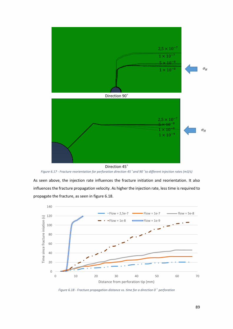
89
Direction 90°
Direction 45°
Figure 6.17 - Fracture reorientation for perforation direction 45° and 90° to different injection rates (m3/s)
As seen above, the injection rate influences the fracture initiation and reorientation. It also
influences the fracture propagation velocity. As higher the injection rate, less time is required to
propagate the fracture, as seen in figure 6.18.
Figure 6.18 - Fracture propagation distance vs. time for a direction 0° perforation
0
20
40
60
80
100
120
140
0 10 20 30 40 50 60 70
Tim
e si
nce
fra
ctu
re in
iati
on
(s)
Distance from perforation tip (mm)
Flow = 2,5e-7 Flow = 1e-7 flow = 5e-8
Flow = 1e-8 Flow = 1e-9
2,5 × 10⁻⁷
2,5 × 10⁻⁷
1 × 10⁻⁷
5 × 10⁻⁸
1 × 10⁻⁸
1 × 10⁻⁸ 5 × 10⁻⁸
1 × 10⁻⁹
𝜎𝐻
𝜎𝐻

90
As seen in figure 6.18, even for direction 0°, for the lower studied flow rate, the fracture was
able to initiate, however it was unable to propagate in distance. This happen because the
generated pressures at the fracture tip are inferior to the tensile strength of the rock and the
failure criteria is not satisfied.
6.8 Different phasing
As already stated in this document, the perforation phasing is selected to ensure that with few
degrees difference, there is a perforation in the direction of greatest principal stress 𝜎𝐻, and
usually the use of a higher perforation density means a higher uncertainty regarding the in-situ
principal stress directions.
In this sense the following perforations phasing are analysed: 60°, 90°, 120° and 180° (i.e. the
base case). According to equation 3.55, in the presence of various perforations, the flow is
divided equally by the number of perforations. Therefore, the perforation phasing influences
the results, once the flow rate was found to be one of the most important parameters for
oriented perforation initiation and propagation.
Figure 6.19 shows the fracture reorientation for the different phasing.
60° Phasing 90° Phasing
𝜎𝐻
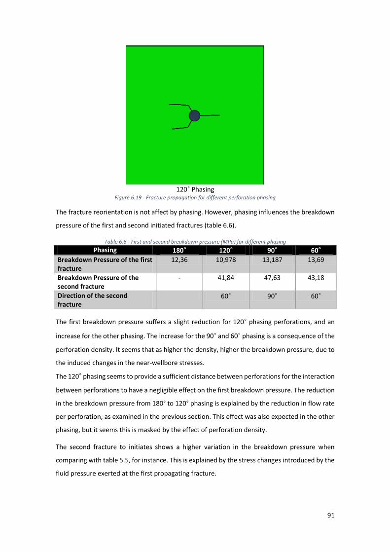
91
120° Phasing
Figure 6.19 - Fracture propagation for different perforation phasing
The fracture reorientation is not affect by phasing. However, phasing influences the breakdown
pressure of the first and second initiated fractures (table 6.6).
Table 6.6 - First and second breakdown pressure (MPa) for different phasing
Phasing 180° 120° 90° 60°
Breakdown Pressure of the first fracture
12,36 10,978 13,187 13,69
Breakdown Pressure of the second fracture
- 41,84 47,63 43,18
Direction of the second fracture
60° 90° 60°
The first breakdown pressure suffers a slight reduction for 120° phasing perforations, and an
increase for the other phasing. The increase for the 90° and 60° phasing is a consequence of the
perforation density. It seems that as higher the density, higher the breakdown pressure, due to
the induced changes in the near-wellbore stresses.
The 120° phasing seems to provide a sufficient distance between perforations for the interaction
between perforations to have a negligible effect on the first breakdown pressure. The reduction
in the breakdown pressure from 180° to 120° phasing is explained by the reduction in flow rate
per perforation, as examined in the previous section. This effect was also expected in the other
phasing, but it seems this is masked by the effect of perforation density.
The second fracture to initiates shows a higher variation in the breakdown pressure when
comparing with table 5.5, for instance. This is explained by the stress changes introduced by the
fluid pressure exerted at the first propagating fracture.

92
Comparing the breakdown pressure of the second fracture for 120° and 60° phasing, the 60°
phasing breakdown pressure is higher than the 120° phasing. Once again, this may be explained
by the perforations density and its influence in the near-wellbore stress state.
Another possibility and closer to the reality is to use these same phasing slightly misaligned with
the PFP.
6.9 Phasing misalignment
This study was executed with a misalignment of 15° to the preferred fracture plane, with the
results presented in figure 6.20.
60° Phasing 90° Phasing
120° Phasing
Figure 6.20 - Fracture propagation for different phasing with perforation miss alignment
The first and second fracture breakdown pressures are presented in table 6.7.
𝜎𝐻

93
Table 6.7 - First and second breakdown pressure (MPa) for different phasing
Phasing 180° 120° 90° 60°
Breakdown Pressure of the first fracture
15,85 14,853 17,714 20,118
Breakdown Pressure of the second fracture
- 46,97 52,15 40,06
Direction of the second fracture
75° 75° 45°
The results are similar to those seen in section 6.8 for perforation phasing aligned with PFP
phasing; The first breakdown pressure for 180° phasing is higher than that for 120° phasing, but
lower than for 90° and 60° phasing.
This corroborates the results obtained in section 6.8. The influence area of the perforation is
insufficient for the 120° phasing to affect significantly the stress state in the surrounding of the
other perforation.
The second breakdown pressure also suffers a higher increase in comparison with the first.
Comparing the second breakdown pressure for 90° and 120° phasing, the higher perforation
density causes an increase in the pressure required to generate the rock tensile failure.
The increase in the second fracture breakdown pressure is coherent with the reality, once the
oriented perforation objective is to create a single and wide fracture, to increase the productivity
of the well. The second fractures at more deviated from the PFP and thus are expected to have
smaller widths, at least for small injected volumes, which may reduce the cost-benefit of the
operation.

94
7. Conclusions and future work
Due to the high cost of a Hydraulic fracturing operation, pre-design is essential to maximize the
economic potential of the reservoirs. The determination of the in-situ principal stresses has a
high degree of uncertainty, and the use of oriented perforations with different phasing ensures
the initiation and propagation of single fractures in controlled conditions.
To understand the fracture initiation and propagation mechanism is essential to study the
mechanics of the materials involved: rock, fluid and fracture. This information together with the
understanding of the basis of the XFEM is essential to better understand and analyze the
simulation results.
Initially a numerical study to validate and explore the capabilities of the software and the XFEM
to model propagating fractures was performed. This consisted in the simulation of a fracture
toughness determination test for an infinite plate with a central crack under tension, and a good
match between the numerical results and the theoretical solution has been obtained. This
exercise has allowed the integration of the fracture mechanics concepts and demonstrated that
Abaqus software, and in particular the XFEM functionality, mimics well fracture initiation. It also
allowed to understand some of the XFEM limitations, e.g. stress intensity factors can only be
accessed in a stationary fracture model.
Subsequently, a series of coupled hydro-mechanical numerical analyses were carried out to
simulate the laboratory tests described by Abass H. et al. (1994). Overall, the numerical analyses
were found to reproduce well the observed experimental results. Based on this set of analyses
some conclusion can be drawn:
- The wellbore excavation changes the near-wellbore stress state. This situation
increases the stresses in the proximity of the wellbore, with the effect being negligible
close to the boundaries, where stresses are similar to the confining applied pressure by
the true-triaxial equipment.
- The breakdown pressure increases as the direction of the perforation deviates from
the PFP. This is due to the increase of the local tangential stresses at the crack tip, with
increasing the perforation angle.
- Perforations along non-preferred directions affect significantly the fracture breakdown
pressure and the reorientation procedure. Perforations more deviated from the PFP
perforations tend to have more reorientation difficulties and the breakdown pressure
increase as a consequence of the higher tangential stresses at the crack tip. Fracture

95
initiation for the situation without initial perforation is well reproduced by the numerical
simulations, which corroborates the model representativeness and the capabilities of
the numerical tools.
- The fluid injection generates changes in the tangential stresses around the perforation
tip region of 1-4 MPa, between the excavation of the wellbore and the fracture
initiation.
- Fracture reorientation towards the PFP is dependent on the anisotropy ratio; it is found
that the reorientation radius (i.e. reorientation distance) increases as the direction of
the perforation deviates from the PFP.
- The fracture width reduces with the tortuosity. However, for the conditions examined
in the simulations the tortuosity effect reduces when the injected flow increases,
because the dimensions and properties of the model are not sufficient to accommodate
the total injected volume.
- The equilibrium pressure (i.e. extension pressure) increases as the direction of the
perforation deviates from the PFP. This is explained by the higher tangential stresses at
directions more deviated from PFP. During the simulations some pressure peaks were
felt, which is according with Abass H. et al. (1994) but may also be result of numerical
convergence difficulties.
The results obtained from this set of analyses support the decision to use the same numerical
tools to conduct a representative study on the effect of a set of parameters on hydraulic
fractures initiation and propagation that make use of oriented perforations. From this study
some conclusions can be drawn:
- The permeability affects fracture initiation and the breakdown pressure is found to
increase with higher permeability, independently of the perforation direction. The
increase in permeability facilitates the movement of the fluid within the rock mass,
which increases the tangential stresses at the fracture tip.
- The fracture surface friction coefficient does not affect the breakdown pressure;
however, it affects the fracture reorientation. For perforation directions higher than 45°
with the PFP, the effect of the friction coefficient becomes residual when compared with
the in-situ stress state. For perforation direction lower or equal to 45° with the PFP,
increasing the friction coefficient reduces the pinch effect in the fracture path, which
may cause an increase in the fracture productivity.

96
- Higher stress anisotropy ratios increase the capacity of fracture reorientation, with the
reorientation to the PFP occurring over a smaller distance. The breakdown pressure is
also affected by the stress anisotropy; an increase in stress anisotropy ratio causes a
reduction of breakdown pressure for direction 0° and 45°, and a slight increase in
direction 90°, which is coherent with the near-wellbore equilibrium conditions. The
injected flow that causes fracture initiation is found to decrease for higher values of
stress anisotropy ratios, following a similar trend for directions 0°, 45° and 90°.
- The fracture propagation regime presented herein was a viscosity and storage
dominated propagation regime, and it was expected that the fluid viscosity would affect
significantly the fracture initiation and propagation. However, the injection flow rates
considered in Abass H. et al. (1994) are very high, and thus this becomes the controlling
parameter of the fracture behavior. To verify the viscosity effect an infinite viscosity fluid
was considered and the results showed a great increment in the fracture width, and
small differences in the fracture initiation and propagation.
- For the conditions considered, a reduction in the flow rate leads to a reduction in the
breakdown pressure for direction 0° and 45°, while for direction 90°, as the in-situ
tangential stresses at the perforation tip are higher than for the other directions, the
fluid viscosity has a smaller influence in the near-tip stress state, and the breakdown
pressure is not affected for intermediate injection rates.
- As lower the injection rate, higher is the influence of viscosity in the initiation and
propagation of the fracture. If the effect of viscosity was negligible, the volume of
injected fluid necessary to cause the tensile failure of the rock mass would be
independent of the injection rate; however, it is found that the total injected volume is
reduced when reducing the flow rate, increasing the influence of viscosity in the
initiation and propagation of the fracture. On the other hand, the velocity of fracture
propagation reduces when considering lower injection rates, and for very low injection
rates the fracture is unable to propagate for a significant distance.
- Using a perforation higher density increases the probability of a perforation being
oriented close to the PFP, optimizing the success of a HF operation. The breakdown
pressure of the first fracture (subjected to lower tangential stresses) is not significantly
affected by phasing misalignment; however, the initiation of a second fracture tends to
suffer an increase in the breakdown pressure, which is explained by the stress changes
introduced by the fluid pressure exerted at the first propagating fracture.

97
As explained in the document, the analyses assume that the formation of the wellbore and
perforations was instantaneous and during these operations the rock responded in undrained
conditions, and the injection associated with hydraulic fracturing operations occurred
immediately after, i.e. the excess pore pressures generated during the formation of the wellbore
were not allowed to dissipate. It is acknowledged that this may have influenced the obtained
results. For this reason, the other limit condition, i.e. drained conditions at the start of the
injection operations, should be tested through the consideration of a consolidation period of
say, at least one day, to understand and quantify the effect of the pore pressure regime on the
obtained results.
Due to the sample dimension and the Abass H. et al. (1994) test conditions (i.e. high flow rates),
the analysis of some of the parameters is not representative (e.g. viscosity). To overcome this, a
large-scale numerical model should be considered. This model would also be important to have
the real magnitude of the fracture widths during fracture propagation, once this model is only
able to provide trends.
The use of three-dimensional simulations may provide information on the vertical propagation
of the fracture, and would enable to quantify the consequences of the plain strain assumption
made through this study.
The data retrieved from the parametric study can be used together with other operation
optimization software (as input file), to study the production phase of a hydraulically fractured
well.
This study has improved the understanding of the factors controlling the behavior of oriented
perforation as well as the XFEM numerical tool ability to model hydraulically induced fractures.

98
References
Abass H. et al. (1994). Oriented Perforations - A Rock Mechanics View. New Orleans, Louisiana:
Society of Petroleum Engineers.
Advani H. S. et al. (1991) A fixed grid finite element method for nonlinear diffusion problems
with moving boundaries. Computational Mechanics, Volume 8, Issue 2, pp 111-123
Ahmed A. (2009). eXtended Finite Element Method (XFEM) - Modeling arbitrary discontinuities
and Failure analysis. Pavia, Italia: Instituto Universitario di Studi Superiori di Pavia.
Altmann J., A. (2010). Poroelastic effects in reservoir modelling. Karlsruher Instituts für
Technologie.
Amao A. M. (2007). Mathematical model for darcy forcheimer flow with applications to well
performance analysis. Texas: Texas Tech University.
Anderson T. L. (2005). Fracture Mechanics: Fundamentals and Applications, Third Edition. Boca
Raton: CRC Press-INC.
Arlanoglu C. (2011). Casing Drilling and Modeling of Smear Effect. Austin: The University of
Texas.
Arthur J. D. et al. (2008). Hydraulic Fracturing Considerations for Natural Gas Wells of the
Fayetteville Shale. All consulting.
Arthur J. D. et al. (2009). Environmental Considerations of Modern Shale Gas Development. SPE
Annual Technical Conference and Exhibition. New orleans , Louisiana: Society of
petroleum engineers.
Atukorala D. (1983) Finite element analysis of fluid induced fracture behavior in oilsands. The
university of British Columbia.
Aud W. et al. (1994). The Effect of Viscosity on Near-Wellbore Tortuosity and Premature
Screenouts. SPE Paper 28492, 305-317.
Ayala G. (2006). Variational formulation of the strain localization phenomenon. Mexico: Instituto
de Ingenieria UNAM.
Barenblatt G. I. (1962). Mathematical theory of equilibrium cracks. In Advances in Applied
Mechanics (Vol. Volume 7).
Barsoum R. S., B. (1976). On the use of isoparametric finite elements in linear fracture
mechanics. International Journal for Numerical Methods in Engineering 10, 551-564.

99
Basak P., B. (1977). Non-Darcy flow and its implications to seepage problems. Journal of the
Irrigation and Drainage Division (ASCE).
Behrmann L. A. et Nolte K. G. (1999). Perforating Requirements for Fracture Stimulation. SPE
Paper 59480, 228-234.
Belytschko T. and Black T. (1999). Elastic crack growth in finite elements with minimal
remeshing. International journal for numerical methods in engineering. Volume 45, Issue 5. pp
601-620.
Caldeira L. et Cardoso R. (2013). Finite element method notes for Advanced Geotechnics
Modelling. Lisboa: Instituto Superior Técnico.
Chahine E. et al. (2006). Crack tip enrichment in the XFEM method using a cut-of function.
Internatioanl journal for numericcal methods in engineering.
Charlez A. Ph. (1997). Rock Mechanics: Petroleum aplications (Vol. Volume 2). Éditions Technip.
Chaves E. W. et Oliver J. (2001). On the strong discontinuity approach in 3D setting. 22nd Iberian
Latin-American congress on computational methods in engineering. Campinas, Brasil:
Unicamp.
Chen M. et al. (2010). The Experimental Investigation of Fracture Propagation Behavior and
Fracture Geometry in Hydraulic Fracturing through Oriented Perforations. Taylor &
Francis Group - Petroleum Science and Technology, 1297–1306.
Cherny S. et al. (2009). Two-dimensional modelling of the near-wellbore fracture tortuosity
effect. International Journal of Rock mechanics and Mining Sciences - Elsevier, 992-1000.
Conterato L. (2011). Rochas basálticas: Obtenção dos parâmetros elásticos através do ensaio de
tracção indirecta. Porto Alegre: Universidade federal do Rio Grande do Sul.
Daneshy A. (2010). Hydraulic fracturing to improve production. The Way ahead - Tech 101,
Volume 3 , Number 6.
Dassault Systémes. (2013). Abaqus User's Manual. Providence: Dessault Systémes Simulia Corp.
Dassault Systémes. (2015). Modeling Fracture and Failure with Abaqus. Simulia 3DS. Retrieved
from http://www.3ds.com/products-services/simulia/services/training-
courses/course-descriptions/modeling-fracture-and-failure-with-abaqus/
Detournay E. and Cheng A.H., D. (1993). Fundamentals of Poroelasticity. In Comprehensive Rock
Engineering: Principles, Practice and Projects, Vol. II, Analysis and Design Method. ,
Pergamon Press.

100
Detourney E. et Cheng A. (1991). Plain strain analysis of a stationary hydraulic fracture in a
poroelastic medium. International Journal Solids and Structures, Number 13, 1645-1662.
Duarte A. and Simone A. (2012). An Introduction to Partition of Unity and Generalized Finite
Element Methods. Departament of Civil Enginnering, UNICAMP, Campinas, Brazil.
Duarte C. A. M. and Oden J. T. (1996). A H-p adaptative method using clouds. Computer methods
in applied mechanics and engineering. Volume 139.
Economides M. J. (2010). Best practices for candidate selection, design and evaluation of
hydraulic fractute treatments. SPE Production and Operations Conference and
Exhibition. Tunis, Tunisia: Society of Petroleum Engineers.
Economides M. J. et al. (2000). Reservoir Stimulation. Chicester: John Wiley and Sons.
Economides M. J. et al., E. (1993). Petroleum production Systems. Prentice Hall petroleum
Engineering Series.
EPA. (2004). Evaluation of Impacts to Underground Sources of Drinking Water by Hydraulic
Fracturing of Coalbed Methane Reservoirs - Appendix A. USA: EPA - Department of
energy.
Fink J. (2011). Petroleum engineer’s guide to oil field chemicals and fluids. Elsevier.
Fink J. K. (2013). Hydraulic Fracturing Chemicals and Fluids Technology. Elsevier .
Fischer-Cripps et Anthony C. (2007). Linear Elastic Fracture Mechanics. In Fischer-Cripps et
Anthony C., Introduction to Contact Mechanics (pp. 31 - 48). Springer - Mechanical
Engineering Series.
Fjaer E. et al. (2008). Petroleum related rock mechanics. 2nd Edition. Elsevier
Fleming M. et al. (1997). Enriched element-free galerkin method for crack tip fields.
International journal for numerical methods in engineering Vol. 40, 1483-1504.
Frantz H. J. et Jochen V. (October 2005). Shale gas: When Your Gas Reservoir is Unconventional,
So is Our Solution. Schlumberger.
Frash L. P. et al. (2014). True-triaxial apparatus for simulation of hydraulically fractured multi-
borehole hot dry rock reservoirs. International Journal of Rock Mechanics & Mining
Sciences, 496-506.
Freeman C. M. et al. (n.d.). A numerical study of microscale flow behaviour in tigth gas and shale
gas reservoir system. Transport in Porous Media, Volume 90 (Issue 1), 253-268.

101
Frydman M. and Fontoura S. (1997) Numerical modeling of borehole pressurization.
International Journal of Rock mechanics and Mining Sciences
Garcia J.G. and Teufel, L.W.(2005) Numerical Simulation of Fully Coupled Fluid Flow. New Mexico
Inst. Of Mining and Technology.
Gidley J. et al. (1989). Recent advances in Hydraulic fracturing (Vol. V.12). SPE Monograph Series.
Gidley J. L. et al. (1989). Fracturing Fluids and Additives. In Recent Advances in Hydraulic
Fracturing (Vol. SPE Monograph Series Vol. 12). Society of Petroleum Engineers.
Gigliotti L. (2012). Assessment of the applicability of XFEM in Abaqus for modeling crack growth
in rubber. Stockholm, Sweden: KTH School of Engineering Sciences.
Griffith A. A. (1920). The Phenomena of Rupture and Flow in Solids. Philosophical transactions /
Royal Society of London. Series A. Containing papers of a mathematical or physical
Character Volume 221, 163-198.
Gross D. et Seelig T. (2011). Fracture mechanics: With an Introduction to Micromechanics ,
Second Edition. Heidelberg Dordrecht London New York: Springer.
Guo B. et al. (2007). Petroleum Production Engineering : a computer assited approach. Elsevier
Science & Technology Books.
Guo T. et al. (2014). Experimental study of hydraulic fracturing for shale by stimulated reservoir
volume. Fuel - Elsevier, 373-380.
Harris P. C. (1988, October). Fracturing-Fluid Additives. Journal of Petroleum Technology, 1277-
1278.
Hatzor Y. H. (2015). Deichmann Rock Mechanics Laboratory. Israel: Ben-gurion university of the
negev. Retrieved from
http://in.bgu.ac.il/teva/geological/eng/hatzor/Pages/Deichmann%20Rock%20Mechani
cs%20Laboratory.aspx
Holditch S. A. (2007). Petroleum Engineering Handbook - Volume IV. Society of Petroleum
Enginners.
Hudson J. A. et Harrisson J. P. (1997). Engineering Rock Mechanics: An introduction to the
principles. Oxford: Pergamon.
Hudson W. R. et Kennedy T. W. (1968). An indirect tensile test for stabilized materials. Austin,
Texas: Center for highway research the University of Texas at Austin.
102
Ibragimov A. et Valko P. (2000). On productivity Index in pseudo-steady state and boundary
dominated flow regime. Texas: Institute for scientific computation - Texas A & M
university.
Inglis C. E. (1913). Stresses in a plate due to the presence of cracks and sharp corners. King's
college, Cambridge.
Itaoka M et al. (2002) Numerical Simulation of geothermal reservoir formation induced by
hydraulic fracturing at great depth.
Jaeger J. C. et Cook N. G. W. (1971). FUndamentals of rock mechanics. London: Chapman and
Hall Ltd.
Karapataki C. (2012). Techno-Economic Analysis of water management options for
unconventional natural gas developments in marcellus shale. Massachussetts:
University of Cambridge and Massachusetts institute of technology (MIT).
Keswani K. et al. (2012). Computation of SIF and Crack Growth Simulation using XFEM
Techniques. International Conference on Advanced Research in Mechanical Engineering.
King E. G. (2012). Hydraulic fracturing 101: What every representative, environmentalist,
regulator, reporter,investor, university researcher, neighbor and engineer should know
about estimating frac risk and improving frac performance in unconventional gas and oil
wells. SPE Hydraulic fracturing technology conference. The Woodlands, Texas: Society
of petroleum engineers.
King G. E., K. (2012). Thirty years of Shale Gas fracturing: What have we learned? Florence , Italy:
SPE annual technical conference and Exhibition.
Li S. et Simkins Jr. D. C. (2002). Conserving Galerkin weak formulations for computational
fracture mechanics. In Communications in numerical methods in engineering (pp. 835-
850). John Wiley & Sons.
Liu L. et al. (2014). Numerical Simulation of Hydraulic Fracturing in Shale Gas Reservoir. The
Electronic Journal of Geotechnical Engineering, 17603-17613.
Lu L. J. (2004) New P3D hydraulic fracturing model based on the radial flow. Journal of Beijing
Institude of Technology.
McNary M. J. (2009). Implementation of the extended finite element method (XFEM) in the
abaqus software package. Georgia: Georgia Institute of Technology.
Medinas M. (2015). Hydraulic fracturing: An overview and a geomechanical approach. Lisbon:
Instituto Superior Técnico

103
Melenk J. M. and Babuska I. (1996) The partition of unity finite element method: Basic theory
and applications. Computer methods in applied mechanics and engineering. Volume 139. pp
131-150.
Mohammadi S. (2008). Extended finite element method for fracture analysis of structures.
Oxford: Blackwell Publishing Ltd.
Montegomery C. (2013). Fracturing Fluids. In Bunger P. A. et al., Effective and Sustainable
Hydraulic Fracturing (pp. 3-23). InTech.
Montgomery C. T. et Smith M. B. (2010). Hydraulic Fracturing : History of an enduring
technology. JPT.
Moore L. P. et Ramakrshnan H. (2006). Candidate selection methodologies an treatment
optimization. SPE annual technical conference and exhibition (p. Paper SPE 102681). San
Antonio, Texas , USA: Society of petroleum engineers.
Murdoch L. C. et Slack W. (2002). Forms of hydraulic fractures in shallow fine grained formations.
Journal of Geotechnical and Geoenvironmental engineering, Volume 128, Pages 479-
487.
Natarajan S. et al. (2011). Integrating strong and weak discontinuities without integration
subcells and example applications in an XFEM/GFEM framework. International Journal
for Numerical Methods in Engineering.
Nolen-Hoeksema R. (2013). Elements of Hydraulic Fracturing. In Defining Hydraulic fracturing -
(pp. 51-52). Schlumberger - Oilfield Review.
Oliveira F. (2013). Crack Modelling with the eXtended Finite Element Method. Lisboa: Instituto
Superior Técnico.
Orwan E. (1948). Fracture and Strength of Solids. Reports on Progress in Physics, v. XII.
Pak A. (2008) Numerical Modeling of Hydraulic Fracturing in oil sands.
Paris C. et Sih G. (1964). Stress Analysis of cracks. Bethlehem, Pennsylvania: Lehigh University.
Patrício M. et Mattheij R. M. (2007). Crack Propagation Analysis. Eindhoven: Technische
Universiteit Eindhoven.
Popa A. (2011, December). Application of case-based reasoning for well fracturing planning and
execution. Journal of Natural Gas Science and Engineering, Volume 3(Issue 6), 687-696.
Powell R. J. et al. (1999). Applications of a new, efficient hydraulic fracturing fluid system. In SPE
Production and Facilities (pp. 139-143). Society of petroleum engineers.

104
Raaen A. M. et al. (2001). Stress determination from hydraulic fracturing tests: The system
stiffness approach. International Journal of Rock Mechanics and Mining Sciences,
Volume 38, 529-541.
Rao M. A. (2014). Rheology of fluid, semisolid, and Solid foods - Principles and applications.
Springer.
Rice J. R. (1968). A path independent integral and the approximate analysis of strain
concentration by notches and cracks. Journal of applied mechanics, Volume 35. pp 379-386.
Robbin J. W. (2014). Partitions of Unity Formulation notes. Madison, Wisconsin: University of
Wisconsin.
Romero J. et al. (1995). Theoretical Model and Numerical Investigation of Near-Wellbore Effects
in Hydraulic Fracturing. SPE Paper 30506, 569-578.
Sasaki S. (1998). Sasaki, S., 1998, Characteristics of microseismic events induced during hydraulic
fracturing experiments at the Hijiori hot dry rock geothermal energy site, Yamagata,
Japan. Tectonophysics, Volume 289(1-3), Pages 171–188.
Schlichting H. et Gersten K. (2000). Boundary-Layer Theory. Springer.
Sepehri J. (2014). Application of Extended Finite Element Method (XFEM) to Simulate Hydraulic
Fracture Propagation from Oriented Perforations. Texas: Texas Tech University.
Settari, A. (1989) Physics and modeling of thermal flow and soil mechanics in unconsolidated
porous media. SPE 18420, Houston, Texas
Shin H. (2013). Simultaneous Propagation of Multiple Fractures in a Horizontal Well. Austin: The
University of Texas.
Solyman M. Y. et Boonen P. (1999). Rock Mechanics and stimulation aspects of horizontal wells.
Journal of Petroleum Science and Engineering, 187-204.
Taleghani A. D. (2009). Analysis of hydraulic fracture propagation in fractured reservoirs: an
improved model for the interaction between induced and natural fractures. Austin:
University of Texas at Austin.
Tani I. (1962). Production of longitudinal vortices in the boundary layer along a concave wall
layer along a concave wall. Journal of Geophysical research, 3075–3080.
Thoi T. N. et al. (2015, 01 24). The Computational Mechanics (CM) group. Ho Chi Minh, Vietnam.
Retrieved from http://incos.tdt.edu.vn/index.php/vi/nghien-cuu-hm/114-
computational-mechanics-3

105
Thomas J. et al. (2001). Fundamentos de Engenharia de Petróleo. Rio de Janeiro: Editora
Interciência.
Tie Y. et al. (2011). An experimental study of fracture initiation mechanisms during hydraulic
fracturing. Berlin Heidelberg: Springer-Verlag / China University of petroleum (Beijing).
Valkó P. et Economides M. J. (1995). Hydraulic Fracture Mechanics. Chicester: John Wiley and
Sons.
Varma A. H. (2013). Finite element modelling and analysis : Course Part II. SlideShare.
Veatch R. W. J. et al. (1989). An Overview of Hydraulic Fracturing. In Gidley L. J. et al, Recent
Advances in Hydraulic Fracturing,. Society of Petroleum Engineers - SPE Monograph
Series Vol. 12.
Vermylen J. P. et Zoback M. (2011). Hydraulic Fracturing, microseismic magnitudes, and stress
evolution in the Barnett Shale, Texas ,USA. SPE Hydraulic Fracturing Technology
Conference. The Woodland, Texas: Society of Petroleum Engineers.
Westergaard H. M. (1939). Bearing pressures and cracks. Journal of applied Mechanics, Volume
6. pp A 49-53.
Xiong H. et al. (1996). A Comprehensive Approach to Select Fracturing Fluids and Additives for
Fracture Treatments. SPE Annual Technical Conference and Exhibition. Denver,
Colorado: Society of petroleum Engineering.
Zhang G. et Chen M. (2009). Dynamic fracture propagation in hydraulic re-fracturing. Journal of
Petroleum Science and Engineering, 266-272.
Zhang X. et al. (2011). Initiation and growth of a hydraulic fracture from a circular wellbore.
International Journal of Rock Mechanics and Mining Sciences - Elsevier, 984-995.
Zhen-zhong D. (2009). eXtended Finite Element Method (XFEM) in Abaqus. Dessault Systémes,
Simulia.
Zielonka M. et al. (2014). Development and Validation of Fully-Coupled Hydraulic Fracturing
Simulation Capabilities. 2014 SIMULIA Community Conference.
Zielonka M. G. et al. (2014). Development and Validation of Fully-Coupled Hydraulic Fracturing
Simulation Capabilities. Houston,Texas: ExxonMobil Upstream Research Company -
2014 SIMULIA Community Conference.
Zoback M. (2007). Reservoir Geomechanics. Cambridge: Cambridge University Press.

106
Zoveidavianpoor M. et al. (2012). A review on conventional candidate-well selection for
hydraulic fracturing in oil and gas wells. International journal of engineering and
technology, Volume 2, 51-57.

Annex - A.1 Execution of an Abaqus© XFEM analysis
The XFEM functionality introduces a new and easier way to simulate crack initiation and
propagation. Several different simplifications are essential for fracture implementation. For this
propose, a multi-physics software distributed by Dassault Systémes, Abaqus is selected for the
study carried once it provides the XFEM functionality and all the tools required for an accurate
fracture modelling.
In the following pages are presented the fundaments for the execution of an analysis of a
boundary value problem with Abaqus XFEM, with higher focus to specific subjects related to the
crack analysis.
A 1.1 Abaqus Software structure
The processing of each analysis performed with the aforementioned software is divided into
three distinct phases: pre-processing, simulation, and post-processing. These three processing
stages are inter-connected, wherein in each stage, are produced data files which serves as the
basis for the sequential stage in the processing chain , as seen in Figure A.1. Then are presented
each of these phases:
Figure A.0.1 - Scheme of the interactive processing stages (Author)
Pre-processing (ABAQUS/CAE): At this stage the numerical model is defined conceptually and
formally, as an ABAQUS input file. The model is usually created graphically using the ABAQUS /
CAE (Computer-Aided Engineering / Complete Abaqus Environment), however, depending on
the complexity of the problem/model this may be created using the Keyword edition. Once the
study takes advantage of new features introduced recently, the graphical interface does not
provide all functionalities, so the Keyword edition has used at several stages of the analysis.
Simulation/processing (ABAQUS/Standard): The simulation is the stage where
ABAQUS/Standard solves the numerical model. For instance, the output files of a stress analysis
includes the displacements and stresses that are stored in binary files ready for post-processing.

b
Depending on the complexity of the problem, the input parameters and computer capability, a
simulation can have an ease numerical convergence, produce more or less accurate results and
a diverse computational data consumption. As example to the aforementioned, for the
production of this study, more than 400 GB of CPU memory were used.
Post-processing (ABAQUS/CAE): After the end of the simulation, it is possible to evaluate the
results of displacements, stresses, or other key variables whose calculation has been requested.
The evaluation is usually performed interactively using the visualization module of ABAQUS /
CAE. The visualization module, which reads the binary output database has a variety of options
to represent the results. It is also possible to extract the produced files to Excel, enabling a
broader spectrum of processing and data analysis.
A1.2 Components of the Abaqus Pre-processing phase
An ABAQUS model is composed by different components that together/assembled describe the
physical problem. Depending on the complexity, the number of inputs should vary, however, it
is essential that the model has the following information: geometry, properties of element
section, material data, loads, boundary conditions, analysis type/procedure, and data to be
requested as output.
Geometry and Material properties
The finite elements and nodes define the basic geometry of the physical structure to be modeled
in ABAQUS. Each element in the model represents a discrete portion of the physical structure,
which by is turn, is represented by many interconnected elements. The elements are connected
to each other by shared nodes. The coordinates of the nodes and the connection elements
comprise the model geometry, and constitute a mesh.
Generally, the mesh is only an approximation of the real geometry of the structure. The type,
shape, and position of the element, as well as the total number of elements used in the mesh,
affect the simulation results. The higher the mesh density, i.e., higher number of elements in
the mesh, the more accurate the results. As the mesh density increases, the analysis results
converge into a single solution, increasing the time used by the computer for analysis. However,
the aim is to ensure an approximation to the analytical solution with the lowest possible space
consumption and analysis time. Note that depending on the simplifications made, in the
geometry, material behavior, boundary conditions and loads, is determined how the simulation
approaches the physical problem.
Material properties should be defined for all elements. The ABAQUS has a wide range of element
types. Some limitations are introduced by using XFEM, as explained in the previous chapter.

c
Loads and Boundary Conditions
The loads give rise to distortion and displacement in the physical structure, subsequently
computed as stresses in the body. The Load types used throughout this document include:
Concentrated forces;
Surface pressures;
Fluid concentrated pressure
The boundary conditions are used to constrain the moving parts of the model to remain
stationary or to have a pre-defined displacement. From the analysis point of view, if possible, to
apply a controlled displacement rather than a load/pressure allow to retain better the material
behavior (Hudson J. A. et Harrisson J. P., 1997) , as can be seen in figure A.2.
Figure A.0.2 – Stress (left) and strain (right) controlled stress-strain curves (Hudson J. A. et Harrisson J. P., 1997)
In a static analysis the boundary conditions should be defined in order to constrain the rigid
body displacement of the model, reducing the convergence difficulties.
Output Data
An ABAQUS simulation generates a large amount of output files. To avoid using excessive disk
space, only output data essential to achieve the desired results should by required, reducing the
space consumption. The XFEM is accompanied by a specific set of outputs that should be
requested to make possible to analyze the fracture accurately (Dassault Systémes, 2015).
A1.3 Abaqus/CAE modules
The ABAQUS / CAE is divided into modules, where each module defines a logical point of the
modeling process. As it progresses from module to module, the model is being created. When
the model is complete, the ABAQUS / CAE creates an input file that will be reviewed. After the
simulation and numerical analysis, the information is returned to ABAQUS/CAE to allow
monitoring of work in progress, generating a file with the output data, where it is possible to
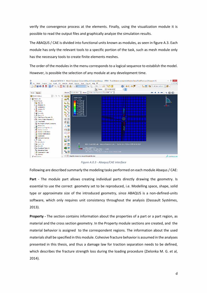
d
verify the convergence process at the elements. Finally, using the visualization module it is
possible to read the output files and graphically analyze the simulation results.
The ABAQUS / CAE is divided into functional units known as modules, as seen in figure A.3. Each
module has only the relevant tools to a specific portion of the task, such as mesh module only
has the necessary tools to create finite elements meshes.
The order of the modules in the menu corresponds to a logical sequence to establish the model.
However, is possible the selection of any module at any development time.
Figure A.0.3 - Abaqus/CAE interface
Following are described summarly the modeling tasks performed on each module Abaqus / CAE:
Part - The module part allows creating individual parts directly drawing the geometry. Is
essential to use the correct geometry set to be reproduced, i.e. Modelling space, shape, solid
type or approximate size of the introduced geometry, since ABAQUS is a non-defined-units
software, which only requires unit consistency throughout the analysis (Dassault Systémes,
2013).
Property - The section contains information about the properties of a part or a part region, as
material and the cross section geometry. In the Property module sections are created, and the
material behavior is assigned to the correspondent regions. The information about the used
materials shall be specified in this module. Cohesive fracture behavior is assumed in the analyses
presented in this thesis, and thus a damage law for traction separation needs to be defined,
which describes the fracture strength loss during the loading procedure (Zielonka M. G. et al,
2014).

e
Abaqus XFEM software assumes the end of cohesive behavior when 𝐺 > 𝐺𝑓 , where 𝐺𝑓 is the
critical fracture energy. The value of 𝐺𝑓 corresponds to the integral of the stress-displacement
diagram, as shown in Figure A.4.
Figure A.0.4 - Energy-based damage evolution for linear softening (Dassault Systémes, 2015)
Where 𝑢𝑓𝑝𝑙
is the displacement to reach the end of cohesive behavior and 𝜎𝑦0 is the tensile
strength of the rock.
Given the loading conditions applied in the analysis presented herein, the MAXPS (Maximum
principal stress) failure criterion is adopted. This is mathematically described as:
𝑀𝐴𝑋𝑃𝑆 = 𝑀𝑎𝑥𝑖𝑚𝑢𝑚 𝑝𝑟𝑖𝑛𝑐𝑖𝑝𝑎𝑙 𝑠𝑡𝑟𝑒𝑠𝑠 = 𝑓 = {
⟨𝜎𝑚𝑎𝑥⟩
𝜎𝑚𝑎𝑥0 }
(A.1)
Where 𝜎𝑚𝑎𝑥 is the stress at a specific point, 𝜎𝑚𝑎𝑥0 is the tensile strength of the rock and the
symbol ⟨ ⟩ is the Macaulay bracket that is used to ensure that a compressive stress state does
not initiate damage, and a fracture is initiated or the length of an existing fracture is extended
by tensile stresses, when the fracture criterion, 𝑓, reaches the value 1,0 within a specified
tolerance:
1,0 < 𝑓 < 1,0 + 𝑓𝑡𝑜𝑙
(A.2)
Where 𝑓𝑡𝑜𝑙 is the tolerance for the initiation criterion. As the simulation of fracture propagation
can be relatively instable, most authors (Dassault Systémes, 2015) propose a value of 0,2 for the
tolerance, and that is the value adopted in the analysis shown here.
The rock strength degradation/damage evolution (i.e. softening behavior) begins when the
failure criterion is verified and progresses linearly until total damage and loss of the section
cohesive behavior is reached.
Assembly - When creating a part, there is a different coordinate system independent of the
other parts of the model. The assembly module is used to assemble the parts and position them
in relation to a global coordinate system, thus creating a set. If the fracture is defined as an

f
individual entity, it should be assembled. If it is modeled as a seam, may be modeled as a portion
of the model geometry. The seam representation is more suitable to use when modeling
stationary fractures.
Step - The step module is used to create and configure the analysis stages/steps, as well as the
requested output data. It provides a convenient way of monitoring changes made to a model
(such as the loading condition and boundary conditions through different steps). To ensure the
results analysis by the user in a more systematically way, various steps should be defined in
stress or deformation increments and shorter periodizations. This facilitates the numerical
calculation process and the results convergence.
Interaction - In this module are specified the mechanical interactions between different regions
of a model or between a region of a model and its neighbors, i.e. between the fracture and the
surrounding region. ABAQUS/CAE does not recognize the mechanical contact between parts or
Assembly regions, unless it is specified in the contact interaction module, since the physical
proximity of two surfaces in the assembly is not sufficient to indicate some kind of interaction
between the surfaces. Interactions are step-dependent objects, which means that should be
specified the analysis steps in which they are active. This module allows the introduction of
cohesive fracture behavior, damage laws, fracture initiation criterion through the technique of
VCCT or surface friction. Note however that when considering a cohesive behavior and traction
separation law for all geometry in the study, the behavior is closer to reality then considering
only a fracture cohesive behavior.
Loads - Load module allows to specify the load, the boundary conditions, and the predefined
fields. The directions of the loads should be checked throughout the process and based on the
program's specifications; it takes tractions as positives and compressions as negatives, by
following the solid mechanics and not the conventions of soil and rocks mechanics. When using
fluids loads on surfaces, this feature is not yet available for XFEM analysis, so its edition must be
made using Keyword edition, taking advantage of the concept of phantom nodes.
In this implementation, each enriched pressure diffusion/stress element (CPE4P) is internally
duplicated with the addition of corner phantom nodes, as seen in figure A.5. Prior to damage
initiation only one copy of the element is active. Upon damage initiation the displacement and
pore pressure degrees of freedom associated with the corner phantom nodes are activated and
both copies of the element are allowed to deform independently, pore pressures are allowed to
diffuse independently, and the created interface behavior is enforced with a traction separation
cohesive law.

g
Figure A.0.5 - Phantom nodes due to pore pressure extra degrees of freedom (original nodes are represented with
full circles and corner phantom nodes with hollow circles) (Zielonka M. G. et al, 2014)
For the XFEM model, the corner phantom nodes on the symmetry surfaces and boundary
surfaces are constrained to move within these surfaces, as seen in figure A.6.
Figure A.0.6- Displacement boundary conditions for the XFEM modelling (Zielonka M. G. et al, 2014)
The fracturing fluid pressure degrees of freedom are associated with the mid-edge nodes of the
cohesive elements and the edge phantom nodes of the enriched elements. Therefore,
concentrated fracturing fluid flow must be applied directly to these mid-edge and phantom edge
nodes, as seen in Figure A.7.
Figure A.0.7 - Concentrated flow injection in the phantom nodes/edge (Zielonka M. G. et al, 2014)
Comparing the analytical models presented previously (see chapter fracture mechanics), the
assumption of a flow injected at fracture level is valid since the leak-off into the surrounding
fluid is null or negligible. Since it is only taken into account a numerical fluid leak-off fluid at the
fracture contact surface, this simplification is consistent.
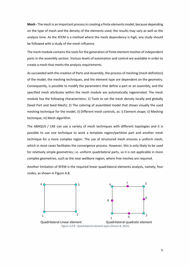
h
Mesh - The mesh is an important process in creating a finite elements model, because depending
on the type of mesh and the density of the elements used, the results may vary as well as the
analysis time. As the XFEM is a method where the mesh dependency is high, any study should
be followed with a study of the mesh influence.
The mesh module contains the tools for the generation of finite element meshes of independent
parts in the assembly section. Various levels of automation and control are available in order to
create a mesh that meets the analysis requirements.
As succeeded with the creation of Parts and Assembly, the process of meshing (mesh definition)
of the model, the meshing techniques, and the element type are dependent on the geometry.
Consequently, is possible to modify the parameters that define a part or an assembly, and the
specified mesh attributes within the mesh module are automatically regenerated. The mesh
module has the following characteristics: 1) Tools to set the mesh density locally and globally
(Seed Part and Seed Mesh); 2) The coloring of assembled model that shows visually the used
meshing technique for the model; 3) Different mesh controls, as: i) Element shape; ii) Meshing
technique; iii) Mesh algorithm.
The ABAQUS / CAE can use a variety of mesh techniques with different topologies and it is
possible to use one technique to work a template region/partition part and another mesh
technique for a more complex region. The use of structured mesh ensures a uniform mesh,
which in most cases facilitates the convergence process. However, this is only likely to be used
for relatively simple geometries; i.e. uniform quadrilateral parts, so it is not applicable in more
complex geometries, such as the near wellbore region, where free meshes are required.
Another limitation of XFEM is the required linear quadrilateral elements analysis, namely, four
nodes, as shown in Figure A.8.
Quadrilateral Linear element Quadrilateral quadratic element Figure A.0.8 - Quadrilateral element types (Forum 8, 2015)
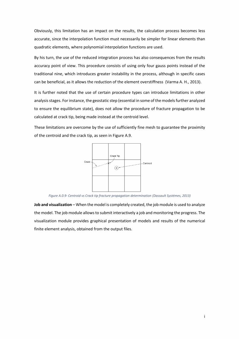
i
Obviously, this limitation has an impact on the results, the calculation process becomes less
accurate, since the interpolation function must necessarily be simpler for linear elements than
quadratic elements, where polynomial interpolation functions are used.
By his turn, the use of the reduced integration process has also consequences from the results
accuracy point of view. This procedure consists of using only four gauss points instead of the
traditional nine, which introduces greater instability in the process, although in specific cases
can be beneficial, as it allows the reduction of the element overstiffness (Varma A. H., 2013).
It is further noted that the use of certain procedure types can introduce limitations in other
analysis stages. For instance, the geostatic step (essential in some of the models further analyzed
to ensure the equilibrium state), does not allow the procedure of fracture propagation to be
calculated at crack tip, being made instead at the centroid level.
These limitations are overcome by the use of sufficiently fine mesh to guarantee the proximity
of the centroid and the crack tip, as seen in Figure A.9.
Figure A.0.9- Centroid vs Crack tip fracture propagation determination (Dassault Systémes, 2013)
Job and visualization – When the model is completely created, the job module is used to analyze
the model. The job module allows to submit interactively a job and monitoring the progress. The
visualization module provides graphical presentation of models and results of the numerical
finite element analysis, obtained from the output files.