An Extension of the ICP Algorithm for ModelingNonrigid Objects with Mobile Robots

Dirk H ahnel†‡, Sebastian Thrun†, Wolfram Burgard ‡†

†Carnegie Mellon University, School of Computer Science, PA, USA,‡University of Freiburg, Department of Computer Science, Germany

Abstract

The iterative closest point (ICP) algorithm[2] isa popular method for modeling 3D objects fromrange data. The classical ICP algorithm rests ona rigid surface assumption. Building on recentwork on nonrigid object models[5; 16; 9], this pa-per presents an ICP algorithm capable of model-ing nonrigid objects, where individual scans may besubject to local deformations. We describe an inte-grated mathematical framework for simultaneouslyregistering scans and recovering the surface config-uration. To tackle the resulting high-dimensionaloptimization problems, we introduce a hierarchi-cal method that first matches a coarse skeleton ofscan points, then adapts local scan patches. The ap-proach is implemented for a mobile robot capableof acquiring 3D models of objects.

1 IntroductionIn recent years, there has been a flurry of work on acquir-ing 3D models from range data. The classical setting in-volves a range sensor (e.g., a 3D range camera or a stereovision system) used to acquire range images of the target ob-ject from multiple vantage points. The problem of integratingmultiple range scans into a 3D model is commonly knownas scan registration. Most state-of-the-art implementationsare based on the populariterative closest pointalgorithm[2].The topic has received significant attention in fields as di-verse as computer vision[12; 9] and medical imaging[7],large-scale urban modeling[14], and mobile robotics[10; 8;15].

ICP aligns range scans by alternating a step in which clos-est points are identified, and a step by which the optimal trans-lation and rotation of scans relative to each other is computed.In doing so, most of them are making a rigid object assump-tion: range scans, if aligned correctly, must be spatially con-sistent with each other.

Many objects are deformable. For example, people changeshape, as do trees, pillows, and so on. A natural researchgoal is therefore to extend ICP to accommodate local objecttransformations. Following recent work primarily found inthe medical imaging literature[5; 16; 6; 3], we proposes anapproach suited for scan registration and 3D modeling of non-rigid objects that can efficiently deal with hundreds of thou-

Figure 1: The essential idea: Rather assuming that the relationof measurement coordinates are fixed relative to the location fromwhich the measurement was taken, the approach proposed here con-straints the relation of measurement coordinates in a soft way. Theexact configuration of a scan is calculated while scans are registeredto each other.

sands of variables. To accommodate local deformations, ourapproach transforms scans into Markov random fields, wherenearby measurements are linked by a (nonlinear) potentialfunction. All links are soft. They can be bent, but bendingthem incurs a penalty. Figure 1 illustrates this transforma-tion: rigid links between the measurement coordinates and therobot sensor are replaced by soft links between adjacent mea-surement points. The resulting problem of scan registrationunder these soft constraints becomes a high-dimensional op-timization problem with orders of magnitude more variablesinvolved than in regular ICP. We show how to solve this prob-lem via Taylor series expansion (linearization), and then pro-pose a coarse-to-fine hierarchical optimization technique forcarrying out the optimization efficiently.

Our new algorithm is applied to the problem of learning3D models of non-stationary objects with a mobile robot. Wedescribe an implemented robot system that utilizes a modeldifferencing technique similar to the one described in[1] tosegment scans. By acquiring views of the target objects frommultiple sides, our approach enables a robot to acquire a 3Dmodel of a non-stationary object.

2 Scan RegistrationThis section describes a variant of the well-knowniterativeclosest pointalgorithm (ICP)[2] for rigid objects. The al-gorithm alternates two phases, one in which nearest points isidentified, and one in which the distance between all pairs ofnearest points is minimized.

2.1 ScansThe input to the ICP algorithm is a set of 3D scans denoted

d = d1,d2, . . . (1)

(a) mobile robot with scanner (b) scene acquired by scanner (c) result of model differencing

Figure 2: (a) 3D range scan acquired by mobile robot shown in (b). (c) Scene from which the scan in (a) is extracted through backgrounddifferencing.

Each such scandk consists of a collection of 1D range mea-surements, arranged as a 3D “range image”:

dk = d1k, d2k, . . . (2)

Figure 2c shows a typical scan acquired by a robot. Furtherbelow, we will denote the horizontal angle of thek-th rangemeasurement byαk and the vertical one byβk. In our experi-mental setup, scans are obtained by a SICK laser range findermounted on a tilt unit shown in Figure 2a.

The problem of scan registration can be formulated as theproblem of recovering the vantage points from which thescans were taken. In our approach, scans are taken from amobile robot; hence each vantage point is described by threevariables: itsx-y location in Cartesian coordinates and its ori-entationγ:

xk = (xk, yk, γk)T (3)

Herexk denotes the vantage point from which scandk wasacquired. The set of all vantage points will be denotedx.Recovering the vantage pointsx is equivalent to registeringthe scans if one vantage point is (arbitrarily) defined to bex1 = (0, 0, 0)T .

2.2 Measurement ModelScans are registered in world coordinates. To do so, measure-mentsdik must be mapped into 3D world coordinates. Thisis achieved by a projective functionπ, which takes as an ar-gument a range measurement and a vantage point and returnsas its output the corresponding coordinate in 3D world coor-dinates:

π(dik,xk) =

(xk + dik cos(γk + αi) sinβiyk + dik sin(γk + αi) sinβi

z + dik cosβi

)(4)

Hereαi andβi are the orientation of the range measurementdik relative to the sensor. The variablez is the generic heightof the sensor which in our robot system is fixed, but is easilygeneralized to variable heights. For brevity, we will some-times writeπik instead ofπ(dik,xk).

We define the quality of a pairwise scan registration by theprobability representing the likelihoodp(dik) of a range mea-surement under a fixed (hypothetical) registration:p(dik | dl,xk,xl) = (5) max

j|2πΣ|−

12 exp

{− 1

2(πik−πjl)TΣ−1(πik−πjl)

}if πik ∈ Fl

const. if πik 6∈ Fl

This likelihood distinguishes two cases. The first case modelsthe noise in range perception by a Gaussian with a sensor-specific covarianceΣ (usually a diagonal matrix). The mea-surement error under this Gaussian is given by the distancebetween the pointπik under consideration, and the pointjin scandl that maximizes this Gaussian. As is easily to beseen, this pointπjl minimizes the Mahalanobis distance toπik. Thus,πjl is simply the point “nearest” toπik in the scandl underΣ−1.

However, finding the nearest point only makes sense ifπikfalls within the perceptual range of scandl. If πik is oc-cluded, it might be perfectly well-explained by an object notdetectable from the vantage pointxl. This is captured by thesecond case in (5), which applies whenπik lies outside thefree space of scanl. The free space of scanl is denotedFl.It is defined as the region between the robot and the detectedobjects. Ifπik lies outside this region, the measurement prob-ability is assumed to be uniform. The value of this uniformdepends on the range of occluded space, but it plays no rolein the optimization to come; hence we leave it unspecified.

2.3 Registration as Likelihood MaximizationThe goal of scan registration is to determine the vantagepointsx that maximize the joint likelihood of the scansd andx:

p(d,x) = p(d | x) p(x) (6)

The first term of this product is obtained by calculating theproduct over all individual measurement likelihoods, assum-ing noise independence in each measurement:

p(d | x) =∏k

∏i

∏l6=k

p(dik | dl,xk,xl) (7)

The termp(x) in (6) is theprior on the individual vantagepoints (and hence on the registration). The prior of the pointxk is expressed as a Gaussian with meanxk and covariancematrixΨ:

p(x) =∏k

p(xk) (8)

=∏k

|2πΨ|−12 exp

{− 1

2(xk − xk)TΨ−1(xk − xk)

}In our robot system, this prior is obtained from the robot’s 2Dlocalization routines, supplied by a public domain softwarepackage[11].

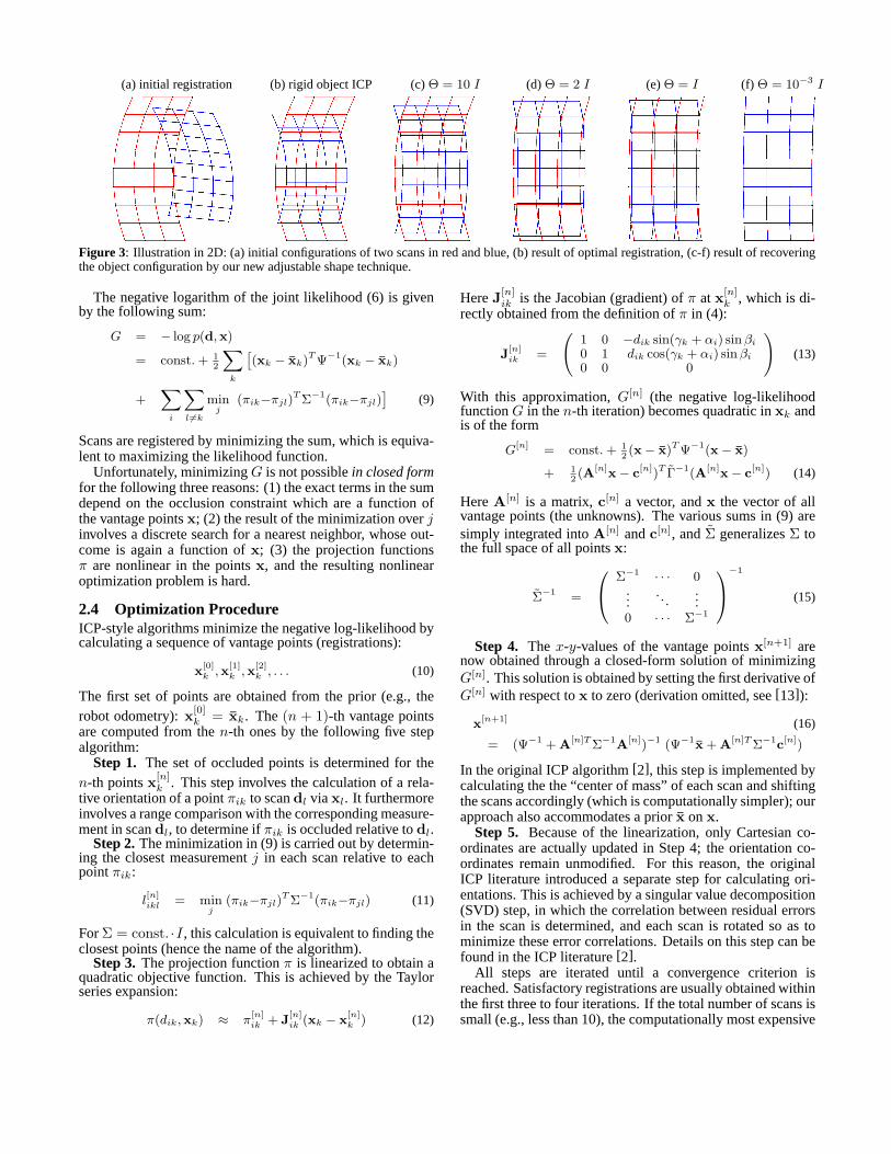
(a) initial registration (b) rigid object ICP (c)Θ = 10 I (d) Θ = 2 I (e)Θ = I (f) Θ = 10−3 I

Figure 3: Illustration in 2D: (a) initial configurations of two scans in red and blue, (b) result of optimal registration, (c-f) result of recoveringthe object configuration by our new adjustable shape technique.

The negative logarithm of the joint likelihood (6) is givenby the following sum:

G = − log p(d,x)

= const.+ 12

∑k

[(xk − xk)TΨ−1(xk − xk)

+∑i

∑l6=k

minj

(πik−πjl)TΣ−1(πik−πjl)]

(9)

Scans are registered by minimizing the sum, which is equiva-lent to maximizing the likelihood function.

Unfortunately, minimizingG is not possiblein closed formfor the following three reasons: (1) the exact terms in the sumdepend on the occlusion constraint which are a function ofthe vantage pointsx; (2) the result of the minimization overjinvolves a discrete search for a nearest neighbor, whose out-come is again a function ofx; (3) the projection functionsπ are nonlinear in the pointsx, and the resulting nonlinearoptimization problem is hard.

2.4 Optimization ProcedureICP-style algorithms minimize the negative log-likelihood bycalculating a sequence of vantage points (registrations):

x[0]k ,x

[1]k ,x

[2]k , . . . (10)

The first set of points are obtained from the prior (e.g., therobot odometry):x[0]

k = xk. The(n + 1)-th vantage pointsare computed from then-th ones by the following five stepalgorithm:

Step 1. The set of occluded points is determined for then-th pointsx[n]

k . This step involves the calculation of a rela-tive orientation of a pointπik to scandl via xl. It furthermoreinvolves a range comparison with the corresponding measure-ment in scandl, to determine ifπik is occluded relative todl.

Step 2.The minimization in (9) is carried out by determin-ing the closest measurementj in each scan relative to eachpointπik:

l[n]ikl = min

j(πik−πjl)TΣ−1(πik−πjl) (11)

ForΣ = const. ·I, this calculation is equivalent to finding theclosest points (hence the name of the algorithm).

Step 3. The projection functionπ is linearized to obtain aquadratic objective function. This is achieved by the Taylorseries expansion:

π(dik,xk) ≈ π[n]ik + J

[n]ik (xk − x

[n]k ) (12)

HereJ[n]ik is the Jacobian (gradient) ofπ at x[n]

k , which is di-rectly obtained from the definition ofπ in (4):

J[n]ik =

(1 0 −dik sin(γk + αi) sinβi0 1 dik cos(γk + αi) sinβi0 0 0

)(13)

With this approximation,G[n] (the negative log-likelihoodfunctionG in then-th iteration) becomes quadratic inxk andis of the form

G[n] = const.+ 12(x− x)TΨ−1(x− x)

+ 12(A[n]x− c[n])T Γ−1(A[n]x− c[n]) (14)

HereA[n] is a matrix,c[n] a vector, andx the vector of allvantage points (the unknowns). The various sums in (9) aresimply integrated intoA[n] andc[n], andΣ generalizesΣ tothe full space of all pointsx:

Σ−1 =

Σ−1 · · · 0...

. . ....

0 · · · Σ−1

−1

(15)

Step 4. The x-y-values of the vantage pointsx[n+1] arenow obtained through a closed-form solution of minimizingG[n]. This solution is obtained by setting the first derivative ofG[n] with respect tox to zero (derivation omitted, see[13]):

x[n+1] (16)

= (Ψ−1 + A[n]TΣ−1A[n])−1 (Ψ−1x + A[n]TΣ−1c[n])

In the original ICP algorithm[2], this step is implemented bycalculating the the “center of mass” of each scan and shiftingthe scans accordingly (which is computationally simpler); ourapproach also accommodates a priorx onx.

Step 5. Because of the linearization, only Cartesian co-ordinates are actually updated in Step 4; the orientation co-ordinates remain unmodified. For this reason, the originalICP literature introduced a separate step for calculating ori-entations. This is achieved by a singular value decomposition(SVD) step, in which the correlation between residual errorsin the scan is determined, and each scan is rotated so as tominimize these error correlations. Details on this step can befound in the ICP literature[2].

All steps are iterated until a convergence criterion isreached. Satisfactory registrations are usually obtained withinthe first three to four iterations. If the total number of scans issmall (e.g., less than 10), the computationally most expensive

step is the determination of the closest points in Step 2. Thisstep is usually implemented efficiently by representing scansthrough kd-trees[4].

Figure 3a-b illustrate the result of scan registration in 2D.The initial configuration in Figure 3a is transformed into theone shown in Figure 3b, which is the one that minimizes thesquared distance (maximizes the likelihood). Clearly, bothscans are incompatible in shape. Pure registration techniquesare unable to handle such shape deformations, but the tech-nique presented in the next section is.

3 Recovering the Surface Configuration ofNonrigid Objects

The key idea for extending ICP to nonrigid objects was al-ready discussed in the introduction to this paper, and is high-lighted in Figure 1. Technically, it involves two modifica-tions: First, the static relationship between pointsπik andthe corresponding vantage pointsxk is replaced by nonrigidlinks between adjacent points. These links can be bent (but ata probabilistic penalty), to accommodate nonrigid surfaces.Second, and as consequence of this, the optimization now in-volves the determination of the location of all pointsπik, inaddition to the robot posesxk. This optimization problem ismuch higher dimensional, and we will discuss a hierarchicaloptimization technique for tackling it efficiently. A key char-acteristic of the approach proposed here is that it fits neatlyinto the ICP methodology above: Again, under appropriatelinearization the target function is quadratic, and estimates areobtained just as in (16).

3.1 LinksThe definition of links between pairs of adjacent points makesit necessary to augment the notion of a measurement point. Inparticular, our approach associates an (imaginary) coordinatesystem with each node. The origin of each coordinate sys-tem is the familiar coordinateπik, and its orientation is speci-fied by three Euler angles (an alternative formulation may usequaternions):

rik = (φik, θik, ψik)T (17)

The orientation is initialized arbitrarily; e.g.rik = (0, 0, 0)T .(The result of the optimization is invariant with respect tothis initialization.) A link is now given by the affine coor-dinate transformations among the coordinate systems of adja-cent measurements. Each link possesses six parameters, threefor rotation (denoted∆ri→j,k) and three for translation (de-noted∆πi→j,k). They are calculated as follows:

∆ri→j,k = rjk − rik (18)

∆πi→j,k = Rz(−ψik) ·Ry(−θik) ·Rx(−φik)

(xjk − xikyjk − yikzjk − zik

)Here theR’s are the rotation matrices around the three coor-dinate axes. Links enable us to recover a node’s coordinatesfrom any of its neighbors:

πjk = πik +Rx(φik) ·Ry(θik) ·Rz(ψik)∆πi→j,k︸ ︷︷ ︸=: πi→j,k

rjk = rik + ∆ri→j,k︸ ︷︷ ︸=: ri→j,k

(19)

To model nonrigid surfaces, our approach allows for violationof these link constraints. This is obtained by introducing thefollowing Gaussian potentials for each link

hi→j,k =; |2πΘ|−12

exp

{− 1

2

(πjk − πi→j,krjk − ri→j,k

)TΘ−1

(πjk − πi→j,krjk − ri→j,k

)}HereΘ defines the strength of the link (the resulting structureis a Markov random field[17]).

3.2 Target FunctionThe negative logarithm of these potentials, summed over alllinks, is given by the following functionH (constant omitted):

H = 12

∑i→j,k

(πjk − πi→j,krjk − ri→j,k

)TΘ−1

(πjk − πi→j,krjk − ri→j,k

)(20)

As in the scan registration problem, all these terms are non-linear in the node coordinatesπik and the orientationsrik.To obtain a closed-form solution for the resulting equationsystem, the link function is linearized via a Taylor series ex-pansion:(

πjkrjk

)≈

(π

[n]ik

r[n]ik

)+K

[n]ik,ik

(πik − π[n]

ik

rik − r[n]ik

)(21)

whereπ[n]ik andr[n]

ik specify the coordinate system for the node

ik in then-th iteration of the optimization. The matrixK [n]ik,ik

is a Jacobian matrix of dimension six by six, which is obtainedas the derivative of the functions (19).

By the same logic by whichG can be approximated by aquadratic function in the scan registration problem, substitut-ing our approximation back into the definition ofH gives us aquadratic function in all variablesπik andrik. This functioncan be written in the form

H = 12

[B[n]

(πr

)− f [n]

]TΘ−1

[B[n]

(πr

)− f [n]

](22)

whereπ is the vector of all coordinate system origins,r thevector of all Euler angles, andB[n] is a matrix andf [n] a vec-tor. CalculatingB[n] andf [n] is involved but mathematicallystraightforward.

3.3 Optimization ProcedureOur new version of ICP now minimizes the combined targetfunctionG + H, which is again quadratic in all parameters(x, π, andr). By doing so, it simultaneously recovers thescan registration and the surface configuration of the object.The solutions forx andπ are completely analogous to the onein (16): (

π[n+1]

r[n+1]

)= (B[n]TB[n])−1 B[n]T f [n] (23)

The global orientation is still optimized by a single globalSVD as above. Our new augmented optimization leads torelative adjustments between measurement points, in whichthe links play the role of soft constraints.

This is illustrated in Figure 3c-f, for different values forΘ. As the various diagrams illustrate, scans are deformed toimprove their match. The degree of the deformation dependson the value ofΘ, which defines the rigidity of the surface.Figure 3c-f illustrates that our approach succeeds in locallyrotating and even rescaling the model.

Figure 4: Example of a thinned graph superimposed to the origi-nal scan left) and before and after adjustment (right). Thinning isnecessary to perform the optimization efficiently.

3.4 Efficient Variable Resolution OptimizationThe main problem with the approach so far is its enormouscomplexity. The number of variables involved in the opti-mization is orders of magnitude larger than in scan registra-tion. This is because the target functionH is a function of allmeasurement pointsπ and orientationsr, whereasG has onlythe vantage pointsx as its arguments. The matrixB[n] in (23)is, thus, a (sparse) matrix with many thousand dimensions.

To tackle such problems efficiently the optimization is re-duced to a sequence of nested optimization problems. In afirst step, scans are analyzed for connected components (re-gions without large disparities); links exist only between con-nected components in each scan; henceH factors naturallyinto different subproblems for different connected compo-nents. Next, the resulting scan patches are thinned. Thin-ning proceeds by identifying a small number of representa-tive landmark measurements that are approximately equallyspaced. This computation is performed by stipulating a gridover the scan (in workspace coordinates), and selecting mea-surements closest to the center points of each grid cell. An allpoint shortest path search then associates remaining measure-ments with landmark measurements. The optimization is firstperformed for the thinned scan; after the landmark scans arelocalized (and the corresponding coordinate transformationare computed), the remaining measurements are optimizedlocally, in groups corresponding to individual landmark mea-surements. Smoothness is attained by using multiple land-mark measurements as boundary conditions in this optimiza-tion. Figure 4 shows an examples of a thinned graph, forwhich the optimization can be carried out in seconds.

4 Setup and Experimental ResultsOur approach was implemented using a mobile robot, in anattempt to acquire 3D models of non-stationary objects. In a

start loop #1 loop #2 loop #3moving armsscan 1 2.3266 0.8993 0.7986 -scan 2 2.5320 0.8704 0.8001 -stretched bodyscan 1 1.9369 1.2915 1.2008 1.1975scan 2 2.5087 1.2964 1.2220 1.2120

Table 1: Average distance to the closest points to the matched modelafter scan registration. The decrease of this distance measures theimprovement of the model through local surface deformations.

Figure 5: 2D map, object (center) and four different vantage points.

technique adopted from[11], we first acquired a map of theenvironment (see Figure 5). Non-stationary objects were de-tected through differencing of scans, using the robot’s local-ization routines to get a rough estimate of this pose. Figure 2billustrates the segmentation process. Red scans are retainedwhile the black scans are assumed to correspond to the back-ground and are henceforth discarded.

Figure 6 illustrates one iteration of the algorithm in all es-sential steps, using data acquired by the robot. Results formatching three scans with different postures are shown in Fig-ure 7(a-b). While the standard registration procedure leads toa model with six arms, our approach correctly deforms thescan to arrive at an improved model, with two arms. A sim-ilar result is shown in Figure 7(c-g), which shows three rawscans on the left, followed by the result of (rigid) scan reg-istration and the result of our approach. Another example isthe chair in Figure 8(a-d) scanned in different heights. Thestandard registration will lead to multiple feet, our approachcorrectly aligns them. Table 1 shows the cumulative distancebetween points in the nearest neighbor calculation. The valuemarked as “start” is the result of an initial registration phase,reflecting the remaining distances under the rigid body as-sumption. All other columns correspond to further iterationsof our algorithm as it adjusts the shape of the scans. This re-sult illustrates numerically the integrity of the result is indeedimproved by iterate the process.

5 DiscussionThis paper proposed a technique for simultaneous scan reg-istration and scan deformation for modeling nonrigid objects.The deformation was made possible through the definition of(soft) links between neighboring scan points, whose config-uration was calculated during registration. To tackle the re-sulting optimization problem efficiently, we described a hi-erarchical optimization techniques that operated on thinnedgraphs. Experimental results obtained using a mobile robotillustrated the viability of this approach.

There are many problems in object modeling that this pa-per does not address, but whose inclusion shall be the subjectof future research. For example, the present segmentation ap-proach is somewhat simplistic: It will fail if more than onenon-stationary object appears in the scene. The approach re-quires deformations to be small, and the target object maynot move very far during acquisition. Objects are not sub-segmented. This will cause difficulties when components ofobjects are adjacent to different other components, or missingentirely, which can happen if components are combined and

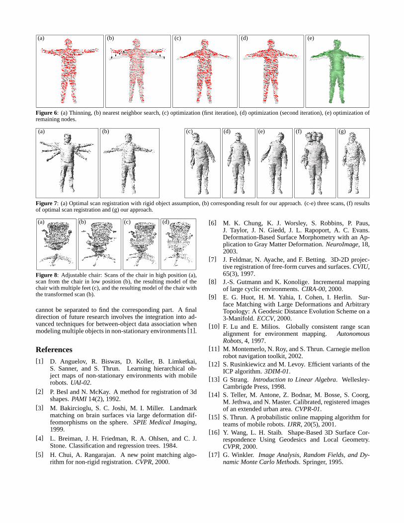
(a) (b) (c) (d) (e)

Figure 6: (a) Thinning, (b) nearest neighbor search, (c) optimization (first iteration), (d) optimization (second iteration), (e) optimization ofremaining nodes.

(a) (b) (c) (d) (e) (f) (g)

Figure 7: (a) Optimal scan registration with rigid object assumption, (b) corresponding result for our approach. (c-e) three scans, (f) resultsof optimal scan registration and (g) our approach.

(a) (b) (c) (d)

Figure 8: Adjustable chair: Scans of the chair in high position (a),scan from the chair in low position (b), the resulting model of thechair with multiple feet (c), and the resulting model of the chair withthe transformed scan (b).

cannot be separated to find the corresponding part. A finaldirection of future research involves the integration into ad-vanced techniques for between-object data association whenmodeling multiple objects in non-stationary environments[1].

References[1] D. Anguelov, R. Biswas, D. Koller, B. Limketkai,

S. Sanner, and S. Thrun. Learning hierarchical ob-ject maps of non-stationary environments with mobilerobots.UAI-02.

[2] P. Besl and N. McKay. A method for registration of 3dshapes.PAMI 14(2), 1992.

[3] M. Bakircioglu, S. C. Joshi, M. I. Miller. Landmarkmatching on brain surfaces via large deformation dif-feomorphisms on the sphere.SPIE Medical Imaging,1999.

[4] L. Breiman, J. H. Friedman, R. A. Ohlsen, and C. J.Stone. Classification and regression trees. 1984.

[5] H. Chui, A. Rangarajan. A new point matching algo-rithm for non-rigid registration.CVPR, 2000.

[6] M. K. Chung, K. J. Worsley, S. Robbins, P. Paus,J. Taylor, J. N. Giedd, J. L. Rapoport, A. C. Evans.Deformation-Based Surface Morphometry with an Ap-plication to Gray Matter Deformation.NeuroImage, 18,2003.

[7] J. Feldmar, N. Ayache, and F. Betting. 3D-2D projec-tive registration of free-form curves and surfaces.CVIU,65(3), 1997.

[8] J.-S. Gutmann and K. Konolige. Incremental mappingof large cyclic environments.CIRA-00, 2000.

[9] E. G. Huot, H. M. Yahia, I. Cohen, I. Herlin. Sur-face Matching with Large Deformations and ArbitraryTopology: A Geodesic Distance Evolution Scheme on a3-Manifold. ECCV, 2000.

[10] F. Lu and E. Milios. Globally consistent range scanalignment for environment mapping. AutonomousRobots, 4, 1997.

[11] M. Montemerlo, N. Roy, and S. Thrun. Carnegie mellonrobot navigation toolkit, 2002.

[12] S. Rusinkiewicz and M. Levoy. Efficient variants of theICP algorithm.3DIM-01.

[13] G Strang. Introduction to Linear Algebra. Wellesley-Cambrigde Press, 1998.

[14] S. Teller, M. Antone, Z. Bodnar, M. Bosse, S. Coorg,M. Jethwa, and N. Master. Calibrated, registered imagesof an extended urban area.CVPR-01.

[15] S. Thrun. A probabilistic online mapping algorithm forteams of mobile robots.IJRR, 20(5), 2001.

[16] Y. Wang, L. H. Staib. Shape-Based 3D Surface Cor-respondence Using Geodesics and Local Geometry.CVPR, 2000.

[17] G. Winkler. Image Analysis, Random Fields, and Dy-namic Monte Carlo Methods. Springer, 1995.