An improve d water correction function for Picarro ... · PDF file1 An improve d water correction function for Picarro greenhouse gas analyzers Friedemann Reum 1, Christoph Gerbig

1

An improved water correction function for Picarro greenhouse gas analyzers Friedemann Reum1, Christoph Gerbig1, Jost V. Lavric1, Chris W. Rella2 and Mathias Göckede1 1Max Planck Institute for Biogeochemistry, Jena, Germany 2Picarro Inc., Santa Clara, CA, USA 5

Correspondence to: Friedemann Reum ([email protected])

Abstract. Measurements of dry air mole fractions of atmospheric greenhouse gases are widely used in inverse models of

atmospheric tracer transport to quantify the sources and sinks of the gases. The measurements have to be calibrated to a

common scale to avoid bias in the inferred fluxes. The World Meteorological Organization (WMO) has set requirements for

the inter-laboratory compatibility of atmospheric greenhouse gas measurements to ±0.1 ppm for CO2 (Southern hemisphere 10

±0.05 ppm) and to ±2 ppb for CH4. An established series of devices for measurements of greenhouse gas (GHG) mole

fractions are the trace gas analyzers manufactured by Picarro, Inc. These have been shown to deliver dry air mole fractions

with accuracies within the WMO goals when trace gas signals are measured in wet air and the effects of water vapor are

corrected for. Here, we report for the first time on sensitivity of the pressure inside the measurement cavity of Picarro GHG

analyzers to water vapor. This sensitivity induces biases in the inferred dry air mole fractions of CO2 and CH4 if they are 15

obtained using the traditional water correction function. To correct for the pressure effect, we add a pressure-related term to

the traditional water correction function, and consider differences between the traditional and enhanced water correction

function to be biases of the traditional model. The effect primarily affects low water vapor mole fractions from about 0.05 to

about 0.5 %, a domain that has gone undersampled in previous studies of the water correction for Picarro GHG analyzers.

We observed biases up to about 40 % of the WMO tolerances (80 % for CO2 in the southern hemisphere). The magnitude of 20

the effect varied across instruments and appeared to be negligible for some, and our experimental results were more robust

for CH4 than for CO2. Thus, correction coefficients should be determined for each analyzer individually. Applying our

enhanced water correction function improves the accuracy of measurements of dry air mole fractions of CO2 and CH4 in

humid air with Picarro GHG analyzers on a scale important for keeping the measurement accuracy within the WMO

requirements. 25

1 Introduction

Measurements of atmospheric GHG mole fractions are integral data for quantifying the sources and sinks of the gases using

inverse models of atmospheric transport (e.g. Kirschke et al., 2013; McGuire et al., 2012). Inverse models require

atmospheric measurements calibrated to a common scale, because relative biases in the mole fraction data lead to biases in

Atmos. Meas. Tech. Discuss., https://doi.org/10.5194/amt-2017-174Manuscript under review for journal Atmos. Meas. Tech.Discussion started: 7 June 2017c© Author(s) 2017. CC BY 3.0 License.

2

the inferred fluxes. The World Meteorological Organization (WMO) has set compatibility goals for atmospheric CO2 and

CH4 measurements to ±0.1 ppm for CO2 (±0.05 ppm in the southern hemisphere) and ±2 ppb for CH4 (WMO, 2016).

In models of atmospheric greenhouse gas transport, the relevant atmospheric information is the dry air mole fraction, i.e. the

number of molecules of the target gas divided by the number of air molecules, not including water vapor. Water vapor is

excluded because its large variability would cover any signal in the trace gases. To measure dry air mole fractions in the 5

humid atmosphere, there are two strategies: (i) drying the air before measurement and (ii) measuring the wet air signal and

correcting for the effects of water vapor later. There are a variety of techniques to dry sample air, including cooling or

streaming it through a nafion membrane dryer. Limitations of this strategy include maintenance requirements, minimum

limits to the achievable dryness, and possibly effects of drying on the GHG mole fractions (Rella et al., 2013).

GHG analyzers manufactured by Picarro Inc. (Santa Clara, CA), which are based on the cavity ring-down spectroscopy 10

technique (Crosson, 2008), are used at many sites of the international GHG monitoring network because of their signal

stability. When using these instruments, the practice is often not to dry the sample air, but instead to measure wet air mole

fractions and subsequently correct for the effects of water vapor. Cavity ring-down spectroscopy is based on absorption of

laser light by the target gas inside a resonator cavity. Active temperature and pressure control in the cavity are built-in to

establish the stable measurement conditions necessary for fitting absorption line shapes. To obtain dry air mole fractions, a 15

water correction function is applied to CO2 and CH4 signals measured in wet air. The established form of the water

correction function accounts for the dilution effect of water vapor and its effects on the shapes of the absorption lines (Chen

et al., 2010; Rella et al., 2013). Dilution changes the target gas mole fraction linearly, and the effects of line shape changes

on the mole fraction measurements are modeled as a second-degree Taylor series. Thus, the overall shape of the traditional

water correction function is a parabola (with a dominant linear term and a small quadratic correction), by which measured 20

wet air mole fractions are divided to obtain dry air mole fractions. By using these functions, water vapor effects on CO2 and

CH4 can be corrected with residuals below the WMO goals. Better accuracy is achieved by determining individual

coefficients for the water correction function specific to each analyzer (Chen et al., 2010; Rella et al., 2013).

Here, we report systematic biases of dry air mole fractions inferred using the traditional parabolic water correction functions

that, to our knowledge, have not been investigated yet. In some cases, the observed systematic deviations were as high as 25

about 40 % of the WMO tolerances (80 % for CO2 in the southern hemisphere). The largest deviations were at low H2O mole

fractions around from about 0.05 to about 0.5 %. We found that only few measurement points at such low water vapor mole

fractions were sampled in previous studies (Chen et al., 2010; Nara et al., 2012; Rella et al., 2013; Winderlich et al., 2010).

In this study, we address the systematic deviations introduced by the traditional water correction function, and find that they

can be explained by a dependency of the pressure inside the measurement cavity on the water vapor content in the sample 30

air. We present a method to correct for the pressure effect, and quantify the impact this correction has on observations from

the field.


3

2 Methods

2.1 Experiments

To determine the effect of water vapor on CO2 and CH4 measurements, dry air from pressurized gas tanks was humidified

and measured with a Picarro GHG analyzer. Pressure in the measurement cavity of the analyzer was monitored with both the

built-in internal pressure sensor and an additional external pressure sensor (Fig. 1). 5

To humidify the air stream, two different methods were used. The first approach was designed to allow stable maintenance

of defined levels of the water vapor content. The dry air stream was split into two lines, one of which remained untreated.

Air in the other line was directed through a gas washing bottle (glass) containing deionized water (depending on bottle size,

about 15 ml to about 500 ml were used in the experiments presented here). Thus, air in this line was saturated with water

vapor (mole fraction about 3 %). Subsequently, the two lines were joined again. The water vapor mole fraction in the re-10

joined line was controlled by adjusting the flow through the wet and dry lines using needle valves. For one of the

experiments (Picarro #1, see Table 1), instead of using the gas washing bottle approach, air was humidified by mixing air

from the gas tank and ambient laboratory air. From this experiment, only pressure data were analyzed.

The second humidification approach was the droplet method. For these experiments, the humidification unit described above

was replaced with a tee piece. To humidify the air, a droplet of deionized water (~ 1 ml) was injected into the line through 15

the tee piece using a syringe. Gradual evaporation of this water droplet then caused a gradient over time from high to low

water vapor levels in the sample air.

Pressure inside the measurement cavity of Picarro GHG analyzers is kept stable by a feedback loop between a pressure

sensor (General Electric NPC-1210) that is mounted inside the cavity, and the outlet valve of the cavity (inlet valve in so-

called Flight-ready Picarro GHG analyzers, which are customized for airborne measurements). With this loop, the cavity 20

pressure is kept stable at 140 Torr. Since Picarro reports cavity pressure in Torr, we will use this unit throughout this paper

(1 Torr = 133.3224 Pa). In our experiments, pressure in the measurement cavity was monitored with an external pressure

sensor (General Electric Druck DPI 142) as well as with the internal sensor. To shield the external sensor from humidity

changes, it was installed in a dead end branched from the main line behind a drying cartridge filled with magnesium

perchlorate. The pressure measurement line was branched directly upstream of the Picarro GHG analyzer (downstream for 25

Flight-ready analyzers). To match the pressure inside the cavity to within a few Torr, a needle valve was installed as a choke

upstream of the pressure measurement branch (downstream for Flight-ready analyzers). This setup allowed us to monitor

pressure independently of water vapor content, while the internal pressure sensor still reacted to changes in water vapor

levels in the sampling air.

The external pressure readings drifted on a timescale relevant for the gas washing bottle experiments. Therefore, in these 30

experiments, dry air was measured between different water vapor levels to calibrate the external pressure readings. Each

water vapor level (including dry air) was probed between 15 and 150 minutes (median about 40 minutes) depending on the

stability of the external pressure measurement and trace gas readings. For further analysis, average readings from the Picarro


4

GHG analyzer and the external pressure sensor of the last 10 minutes of each probing interval were used. Some

measurements with low water vapor levels with probing times of only about five minutes from an early experiment (Picarro

GHG analyzer #1, see Table 1) were included as well. The order of water vapor levels was altered between experiments,

including varying from wet to dry, dry to wet, and random switches between dryer and wetter air.

Experiments were performed with five Picarro GHG analyzers (Table 1). 5

2.2 Traditional parabolic water correction function

The effect of water on trace gas measurements made using Picarro GHG analyzers can be described by a water correction

function 𝑓! ℎ , where 𝑐 denotes the target gas (here: CO2 or CH4) and ℎ is the water vapor mole fraction (measured by the

Picarro analyzer). The analyzer measures the wet air mole fraction 𝑐!"# ℎ , which is related to the dry air mole fraction 𝑐!"#

by the water correction function: 10

𝒄𝒅𝒓𝒚 = 𝒄𝒘𝒆𝒕 𝒉𝒇𝒄 𝒉

(1)

The traditional form of the water correction function takes into account dilution and line shape effects (details in Sect. 1).

These are described by a second-degree Taylor series, i.e. a parabola:

𝒇𝒄 𝒉 = 𝟏 + 𝒂𝒄 ⋅ 𝒉 + 𝒃𝒄 ⋅ 𝒉𝟐 (2)

The coefficients 𝑎! and 𝑏! can be derived from water correction experiments such as those described in Sect. 2.1.

3 Results

3.1 Links among external pressure measurement, CO2, CH4, H2O and cavity pressure 15

To establish the link among the external pressure measurement, CO2, CH4, and internal cavity pressure for each Picarro

GHG analyzer, the cavity pressure was varied manually using Picarro Inc. software in the range observed when varying

water vapor content. Externally measured pressure, CO2, and CH4 varied linearly with internally monitored cavity pressure,

with similar slopes for all instruments. As an example, the values for Picarro #3 obtained in dry air are shown in Table 2.

The water vapor measurement was not sensitive to cavity pressure. The slopes in wet air (3 % H2O) were measured for 20

Picarro #3 and were very similar to the slopes in dry air (CO2: +5 %, CH4: -2 %, cavity pressure: +1 %). Hence, internal

cavity pressure, CO2 and CH4 were modeled as linear functions of externally measured pressure for subsequent analyses.

3.2 Dependency of cavity pressure on water vapor content

We monitored cavity pressure using an external sensor during gas washing bottle experiments (Sect. 2.1) for three different

Picarro GHG analyzers (Table 1). The pressure readings of the internal pressure sensors were, as expected, stable at 140 Torr 25

with standard deviations of 0.015 Torr or less. To calculate a “corrected cavity pressure” from the external pressure


5

measurement, pressure readings for dry air before and after each wet air measurement were interpolated to the times of the

wet air measurements. The deviations between the wet air pressure values and the interpolated dry air pressure values were

multiplied with the slope described in Sect. 3.1, and added to the dry air cavity pressure of 140 Torr. The corrected cavity

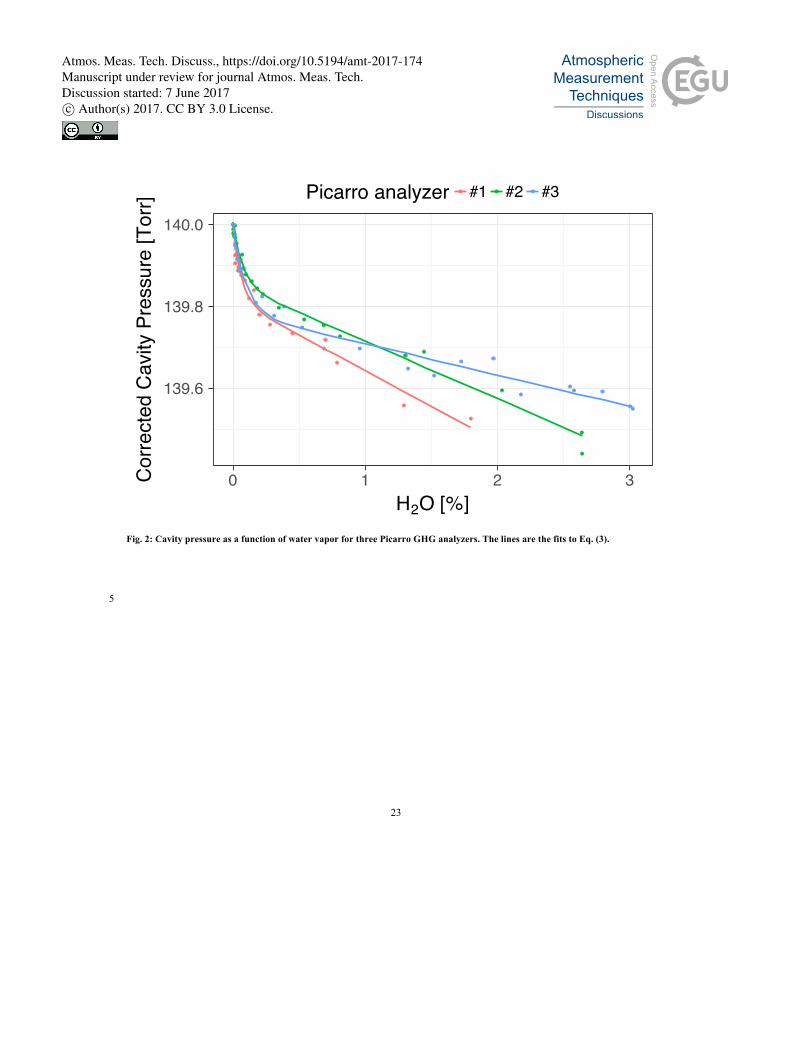
pressure obtained in this way varied systematically with the water vapor mole fraction of the sample air (Fig. 2). The

variations displayed a uniform pattern for all three instruments. The pressure dropped in the presence of water vapor, and the 5

gradient of pressure with respect to water vapor was larger between 0 and about 0.2 % H2O than for higher water vapor

content, exhibiting a “bend” where the two regimes meet. The deviations were up to 0.5 Torr for 3 % H2O.

We describe the relationship between cavity pressure and water vapor mole fraction with an empirical function:

𝒑 𝒉 = 𝒑𝟎 + 𝒔 ⋅ 𝒉 + 𝒅𝒑 ⋅ 𝒆! 𝒉𝒉𝒑 − 𝟏 (3)

10

In this equation, 𝑝 is the cavity pressure as determined from the external pressure measurement, ℎ is the water vapor mole

fraction, ℎ! is the position of the pressure bend described above, 𝑑! is a measure for the pressure gradient at 0 % < ℎ < ℎ!,

𝑝! is the pressure in dry air (fixed at 140 Torr), and 𝑠 is the slope for ℎ ≫ ℎ!. Note that this empirical fit function is valid

only in the water vapor range covered by measurements (see Fig. 2). Data from droplet experiments suggest that the pressure

variation does not continue linearly along the slopes derived here at higher water vapor levels, so an extrapolation is not 15

recommended.

All free parameters of the pressure model (𝑠, 𝑑! and ℎ!) varied between instruments (Table 3). For the empirical water

correction functions for CO2 and CH4, only the pressure bend position (ℎ!) is relevant, as will be shown later. The mean

estimate of ℎ! from all three experiments was (mean and standard deviation):

20

𝒉𝒑 = 𝟎.𝟎𝟕𝟗 ± 𝟎.𝟎𝟏𝟒 % 𝑯𝟐𝑶 (4)

3.3 Correction of the pressure effect on CO2 and CH4

Reliable data for both pressure and the target gases CO2 and CH4 were obtained in one experiment (with Picarro #3), which

is presented in this section. Based on the data, four models were tested as potential water correction functions for CO2 and

CH4 to examine performance, robustness, transferability, and consistency of the results. Model (i) was the traditional

parabolic function, Eq. (2). The other three models represent different strategies to correct for the pressure effect. Model (ii) 25

consisted of first correcting the pressure effect on the wet air mole fractions by estimating the pressure bias from Eq. (3) and

then correcting the trace gas bias using the sensitivity of CO2 and CH4 to pressure (Table 2); then the traditional parabolic

water correction was applied to the corrected wet air mole fractions. For models (iii) and (iv), the traditional parabolic model

was expanded to account for the pressure effect. Since the trace gas readings of the analyzer varied linearly with pressure


6

(Sect. 3.1), the pressure effect was described as in Eq. (2), i.e. as a linear and a non-linear term. Since a linear dependency is

already accounted for in the traditional parabolic model, the non-linear part of Eq. (2) was added to Eq. (3) to obtain a new

model for the water correction:

𝑓!! 𝒉 = 𝟏 + 𝒂𝒄 ⋅ 𝒉 + 𝒃𝒄 ⋅ 𝒉𝟐

𝒇𝒄 𝒉

+ 𝒅𝒄 ⋅ 𝒆! 𝒉𝒉𝒑 − 𝟏 (5)

The parameter 𝑑! describes the magnitude of the pressure change at low water vapor contents and sensitivity of the target

gas to the pressure change. The parameter ℎ! is the pressure bend position from Eq. (3). In model (iii), the parameters 𝑎!, 𝑏!, 5

𝑑! and ℎ! from Eq. (5) were fitted to the trace gas data. Model (iv) was the same as model (iii) except that the pressure bend

position ℎ! was set to the value obtained from the pressure data. Since all free parameters in model (iii) were estimated from

the available trace gas data, this model was the most consistent with the data. Therefore, in subsequent analyses, we assumed

that the fit to model (iii) yielded the true water correction function. Hence, we used the differences between the results from

this model and the others as estimates of their biases. 10

The experiment was performed with dry air mole fractions of 404.0 ppm CO2 and 1842 ppb CH4. Water-corrected CO2 and

CH4 data from this experiment are shown in Fig. 3. For CH4, the most striking visible feature was the wave-like structure in

the dry air mole fractions when using model (i), the traditional parabolic water correction function. The maximum negative

bias of this model was 0.85 ppb at 0.17 % H2O (corresponding to 0.046 % of the dry air mole fraction), and the maximum

positive bias was 0.37 ppb at 1.7 % H2O. Hence, the peak-to-peak difference was 1.2 ppb. The standard deviation of the dry 15

air mole fractions estimated with this model was 0.35 ppb. By contrast, no structure was visible in the dry air mole fractions

calculated with any of the three formulations taking into account the pressure change. This is reflected in the lower standard

deviations of the dry air mole fractions, which were 0.20 ppb for model (ii), 0.17 ppb for model (iii) and 0.18 ppb for model

(iv). This demonstrates the improvement achieved by correcting for the effect of pressure bias on CH4.

The result from model (ii) yielded slightly larger deviations from the mean than models (iii) and (iv) in the range 0.1–0.3 % 20

H2O. These deviations were compatible with a sensitivity of CH4 to cavity pressure changes of 80 % of the value inferred in

Sect. 3.1, since at this value the results from model (ii) resemble the results from model (iv). This discrepancy is discussed in

Sect. 4.3.

The pressure bend position estimated from the CH4 data was ℎ! = 0.059 ± 0.015 % H2O. This is smaller than the

estimate based on pressure data of ℎ! = 0.095 ± 0.011 % H2O. Despite this discrepancy, the two models yielded very 25

similar dry air mole fractions, with differences within 0.12 ppb and a peak-to-peak difference of 0.22 ppb between 0.05 and

0.39 % H2O. This demonstrates the robustness of the method against uncertainties in ℎ!.

The wave-like structure seen in the CH4 dry air mole fractions estimated using the traditional parabolic water correction

function was absent in the CO2 data for this instrument. The standard deviations of the dry air mole fractions were similar for

all models (model (i): 0.017 ppm, model (ii): 0.021 ppm, models (iii) and (iv): 0.014 ppm). 30


7

Using model (ii) induced a bias similar to the one present in the results of model (i) for CH4 but with opposite sign (Fig. 3).

This hints at an overcompensation of the pressure effect on CO2. Indeed, following the same argument as for CH4, the results

of model (iv) were reproduced when the sensitivity of CO2 to cavity pressure changes was set to 35 % of the value presented

in Table 2. Note that the wave-like structure in CO2 was apparent for one other instrument (Picarro #5, see Sect. 3.4 and

3.5.1). This has not been presented in this section since no external pressure sensor data were obtained for this instrument. 5

3.4 Consistency across instruments

To investigate whether common coefficients applicable to all Picarro GHG analyzers can be given for the enhanced water

correction function, we performed water correction experiments with several Picarro GHG analyzers. Although reliable

pressure and trace gas data from a single experiment were obtained for only one instrument (presented in Sect. 3.3), trace gas

data from water correction experiments were obtained for two more analyzers. The pressure effect on the trace gas data from 10

these instruments differed in magnitude. Out of the three instruments for which trace gas data were investigated (Picarros #3,

#4, and #5), two exhibited the pressure effect visibly for CH4 (Fig. 3 and Fig. 5; the exception was Picarro #4, see Fig. 4). In

contrast, the CO2 measurements of two instruments (#3 and #4) seemed to be unaffected by pressure changes (Fig. 3 and Fig.

4; the exception was Picarro #5, see Fig. 5). The differences make clear that common coefficients applicable to all Picarro

GHG analyzers can not be given based on our data. This is further discussed in Sect. 4.3 and Sect. 4.4. 15

3.5 Application to ambient measurements

In this section, we demonstrate the impact that the pressure effect has on ambient GHG observations from a site in northeast

Siberia. The site is located in the remote village of Ambarchik on the coast of the Arctic Ocean (69.62° N, 162.30° E), and

has been operational since August 2014. Air inlets are at 27 m and 14 m above ground level, and probed in turns for intervals

of 15 and 5 minutes, respectively. The gases CO2 and CH4 are measured in the humid air stream with a Picarro G2301 20

analyzer (Picarro #5). The measurements are calibrated automatically by measuring gas tanks calibrated to the WMO scales

X2007 (CO2) and X2004A (CH4) every 116 hours.

3.5.1 Deriving coefficients for the improved water correction function without pressure data

In this section, we derive coefficients for the improved water correction function, Eq. (5), for CO2 and CH4 for the Picarro

G2301 analyzer operated in Ambarchik. For this instrument, one water correction experiment with the gas washing bottle 25

method (see Sect. 2.1) was performed, using dry air from a pressurized tank with mole fractions of 352.9 ppm CO2 and 1797

ppb CH4. Cavity pressure was not monitored during this experiment. We estimated the parameters 𝑎!, 𝑏! and 𝑑! from the

trace gas data (Table 4 and Table 5), but the number of data points was insufficient to also estimate the pressure bend

position ℎ!. Therefore, we used the mean ℎ! from the three experiments with external pressure monitoring, Eq. (4), and

investigated the uncertainty associated with this procedure. 30


8

As a conservative estimate, we considered an interval of three standard deviations around the mean a plausible range for ℎ!,

i.e. ℎ! ∈ [0.036, 0.122] % H2O. Varying ℎ! in small steps within this interval, we fitted the other parameters of Eq. (5) to

the trace gas data. To assess the uncertainty associated to using the mean ℎ!, we assumed that one of the ℎ! yielded the true

water correction function for this instrument, and determined whether using the mean ℎ! could induce a larger error than

using the traditional parabolic correction. For this assessment, we compared not only the data points obtained during the 5

experiment, but sampled the fitted functions at 999 evenly spaced points over the range of H2O covered during the

experiment. For CO2, the maximum deviation between the function using the mean ℎ! and any other ℎ! in the plausible

range was 0.007 ppm, while the best result for the maximum deviation between the traditional parabolic correction and the

improved functions with ℎ! in the plausible range was 0.017 ppm. For CH4, the deviations were 0.20 ppb and 0.35 ppb,

respectively. Therefore, maximum bias due to the uncertainty of ℎ! was smaller than the minimum bias when using the 10

traditional parabolic correction for both CO2 and CH4.

For reference, we also investigated the values for ℎ! estimated from the trace gas data. Fitting Eq. (5) to CH4 yielded

ℎ! = (0.086 ± 0.053) % H2O, close to the mean ℎ! from the three pressure experiments but with a large uncertainty. For

CO2, the fit yielded ℎ! = (0.34 ± 0.19) % H2O, outside of the range considered plausible for ℎ! and again with a very large

uncertainty. It may be argued that the plausible range ℎ! should be extended to 0.34 % H2O. Using this extended range, the 15

argument for the benefit of the improved water correction over the traditional one despite the uncertainty of ℎ! was weaker,

but still held. However, we argue that the estimate ℎ! = 0.34 % H2O is probably far from the true pressure bend position for

this instrument. First, the estimate was based on CO2 data, which were less consistent with pressure data than CH4 data for

another instrument (Sect. 3.3). Second, it is far from the pressure bend positions of all three instruments for which pressure

data were obtained (Sect. 3.2). Third, the estimate was based on very few data points and was not robust against jackknife 20

resampling (not shown). For these reasons, we consider ℎ! from Eq. (4) to be a realistic estimate for this Picarro analyzer.

To assess the bias of the traditional parabolic fit function, we assumed that the fit with pressure correction term using the

mean ℎ! was the true water correction function. Maximum absolute deviations between the two were 0.037 ppm CO2 and

0.78 ppb CH4 at H2O = 0.16 %, and peak-to-peak deviations were 0.052 ppm CO2 and 1.11 ppb CH4 between H2O = 0.18 %

and 1.8 %. These deviations corresponded to biases of 0.0104 % CO2 and 0.0437 % CH4. As an example, for dry air mole 25

fractions of 400 ppm CO2 and 2000 ppb CH4, the maximum absolute bias of the traditional water correction function would

be 0.042 ppm CO2 and 0.87 ppb CH4.

In Sect. 3.3, we compared the sensitivities of CO2 and CH4 to cavity pressure inferred from controlled cavity pressure

changes with those inferred from water vapor changes for Picarro #3. We made the same comparison for Picarro #5 under

the assumptions that the cavity pressure dependency on water vapor and the sensitivities of the trace gases to controlled 30

cavity pressure changes were the same as for Picarro #3. The data from the water correction experiment were compatible

with a sensitivity of CO2 to cavity pressure change of 60 % of the value from controlled cavity pressure changes, which was


9

higher than the 35 % for Picarro #3. The corresponding number for CH4 was 70 %, which more closely matched the 80 % of

Picarro #3.

3.5.2 Impact of the improved water correction

In this section, we describe the impact of the improved water correction on hourly averages of CO2 and CH4 data from

Ambarchik over the years 2015 and 2016. 5

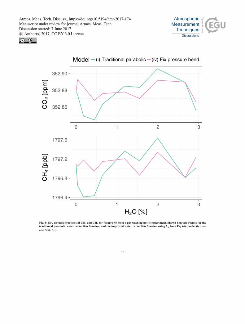
Differences between the traditional and improved water correction had a seasonal cycle following the seasonal cycle of water

vapor content in the sample air (Fig. 6). Maximum water vapor mole fractions occurred in July and August, when they

averaged around 0.9 ± 0.2 %. This was close to the water vapor content where the bias of the traditional parabolic water

corrections changed sign (Fig. 5). Hence, the summer biases averaged 0.00 ± 0.01 ppm CO2 and 0.0 ± 0.2 ppb CH4,

and were thus negligible. In winter, the water vapor content was in the range of the pressure bend position, where the bias 10

was highest. The maximum monthly biases occurred in April and were -0.037 ppm CO2 and -0.75 ppb CH4. From December

to March, water vapor content episodically dropped well below the pressure bend position (this occurred when the air

temperature dropped below about -25°C), thus the bias decreased. During the coldest temperatures, which occurred in

February, the biases were -0.02 ppm CO2 and -0.5 ppb CH4.

We also investigated the effect of the improved water correction on dry air calibrations at this site (data not shown). 15

Calibrations were performed with calibrated dry air gas tanks periodically. The measurement system was flushed with dry air

for at least 13 minutes before data were used. This left so little water vapor in the system that the remaining effects were

negligible.

3.6 Evaluation of droplet experiments for the improved water correction

Droplet experiments are a quick and simple method to obtain data for correcting the influence of water vapor on a Picarro 20

GHG analyzer (Rella et al., 2013). We performed a series of droplet experiments (details on the setup are given in Sect. 2.1)

with Picarro #1, and derived coefficients for the improved water correction function, Eq. (5), for CO2 and CH4. We used data

below 3.5 % H2O and where the difference between subsequent H2O measurements was less than 0.005 %. The latter was an

empirical filter to exclude the fastest water vapor variations while leaving enough data for fitting. The temporal variation of

water vapor during these experiments was fastest during evaporation of the last bits of the droplets, i.e. during the transition 25

from about 0.5–1 % to 0 % H2O (Fig. 7). As determined in the gas washing bottle experiments, this was the domain of

fastest pressure variations, and the pressure during these experiments was consistently too low in this domain, with large

variations between the experiments (Fig. 8). We discuss this deviation in Sect. 4.5.

Consequently, differences between water correction fits were expected. Indeed, the differences between the fit functions for

the different droplets were extremely large around the pressure bend position (0.17 ppm CO2 between droplets 2 and 4 at 30

0.29 % H2O and 6.0 ppb CH4 between droplets 1 and 2 at 0.18 % H2O; Fig. 9). When fixing the pressure bend position to the

value from the gas washing bottle experiment for this instrument (ℎ! = 0.066 % H2O), the scatter increased to 0.24 ppm


10

CO2 and 6.4 ppb CH4. The scatter reduced to 0.04 ppm CO2 and 1.2 ppb CH4 when applying the traditional parabolic fit to

these data, which illustrates that the experiments were consistent apart from the final drop of the water vapor mole fraction to

0 % H2O, where the pressure changed most rapidly.

4 Discussion

4.1 Dependency of cavity pressure on water vapor content 5

Our results demonstrate that the cavity pressure of Picarro GHG analyzers is sensitive to the water vapor content of the

measured air. This effect influences the dependency of CO2 and CH4 on water vapor.

4.1.1 Possible underlying effect

We speculate that the observed sensitivity of internal pressure readings to humidity levels in the sampling air is due to

adsorption of H2O molecules on the pressure sensor inside the cavity. This sensor controls the outlet valve of the cavity (inlet 10

valve for Flight-ready analyzers) to keep the cavity pressure stable. The pressure measurement is based on a piezoresistive

strain gauge exposed to the pressure media (air in the cavity). The strain gauge is mounted on a thin diaphragm, which is

deflected by air pressure. The resulting strain causes a change in electrical resistance and creates an output voltage varying

with pressure. Water molecules adsorbed on the strain gauge, diaphragm, or adjacent parts of the sensor may change its

response to pressure mechanically, and/or may affect the electrical properties of the circuit. If either or both were the case, 15

the deviating pressure readings during droplet experiments could be due to an equilibration time of the adsorption process.

Indeed, the largest pressure deviations were observed when the water content changed fastest (Fig. 7 and Fig. 8). However,

elucidating the underlying physical effect of the pressure changes is beyond the scope of this paper, and was not investigated

further.

4.1.2 Uncertainties of the external pressure measurement 20

The sensitivities of the external pressure measurement to cavity pressure were derived by manually varying cavity pressure

(Sect. 3.1). It is possible that the relationships do not hold for variations of water vapor. One potential influence is the drying

agent in the line of the external pressure sensor, which may affect the sensor readings due to the differences in partial

pressure of water vapor. Additionally, the flow through the needle valves used as chokes to match the external pressure to

cavity pressure may be sensitive to water vapor. 25

To investigate these possible effects, we measured the sensitivity of the external pressure measurement to cavity pressure in

dry and wet air (3 % H2O) for Picarro #3, and found no difference (Sect. 3.1). This indicates that cavity pressure is indeed

well-represented by the external pressure measurement in equilibrium.

Note that, for the empirical correction of the pressure effect on CO2 and CH4, pressure data were used only if the data

obtained in a water correction experiment were insufficient to constrain all parameters of the improved water correction 30


11

function (Sect. 3.5.1). As long as sufficient data are available, uncertainties in our pressure data are of no importance for the

empirical water correction.

4.2 Improvement over traditional parabolic water correction function

As described in Sect. 3.1, CO2 and CH4 depend linearly on pressure. Consequently, the pressure bend (Fig. 2) is featured in

the trace gas data as well. This behavior cannot be modeled with the traditional parabolic water correction function, and 5

hence causes biases in dry air mole fractions derived with the traditional correction. For some instruments, the pressure bend

was visible as water-dependent bias when using parabolas as water correction functions (Fig. 3 and Fig. 5). The improved

water correction function, Eq. (5), resulted in residuals without systematic structure. The bias observed between the

traditional and improved water correction functions was up to 0.037 ppm CO2 (Picarro #5, dry air mole fraction 352.9 ppm)

and 0.85 ppb CH4 (Picarro #3, dry air mole fraction 1842 ppb), with peak-to-peak differences of up to 0.052 ppm CO2 and 10

1.2 ppb CH4, which can appear in ambient air measurements as seasonal cycles or as differences between sites depending on

humidity differences.

To derive water correction coefficients for an instrument, enough data must be available to constrain at least the sensitivity

of CO2 and CH4 to the pressure effect. If not enough data are available to constrain the pressure bend position, it may be

possible to use the mean value from our experiments, ℎ! = 0.079 ± 0.014 % H2O. If this is attempted, one must 15

investigate whether the uncertainty in the pressure bend position may introduce a larger bias than the traditional water

correction function (Sect. 3.5.1).

4.3 Inconsistencies between trace gas- and pressure data

In Sect. 3.3, we found that correcting for the pressure effect on CO2 and CH4 by using the pressure bias and the sensitivities

of the trace gas measurements to cavity pressure during controlled pressure changes (model (ii)) overcompensates the 20

pressure effect. There are two possible explanations: (1) the external pressure measurement may have overestimated the

changes in cavity pressure, or (2) the trace gas mole fractions delivered to the analyzer varied systematically with water

vapor. If explanation (1) were true, the sensitivity of the external pressure sensor reading to controlled cavity pressure

changes (Sect. 3.1) would have been different than to changes due to water vapor. There is no evidence for such an effect

(Sect. 4.1.2). Furthermore, CO2 and CH4 would have been affected in the same way, which was not the case, which makes 25

this hypothesis unlikely. Explanation (2) seems more likely, since overall CO2 results were less robust than those for CH4.

We observed no visible pressure effect at all on CO2 from two out of three instruments (Fig. 3 and Fig. 4). In one of these

instruments (#3), the pressure effect was seen in CH4 in the same experiment (Fig. 3). The fact that CO2 and CH4 behaved

differently suggests that the inconsistent results for CO2 were due to the variations in the mole fraction delivered to the

Picarro analyzer. A difference between the two gases is the higher solubility of CO2 in water, which makes it difficult to 30

deliver a constant CO2 mole fraction to the analyzer under varying humidity. However, we carefully observed the

equilibration of trace gas mole fractions during the experiments. It is possible that an equilibration effect was at play at a


12

time scale much longer than an hour, since this may have gone unobserved in our experiments. If this explanation were true,

the systematic difference between dry air and wet air trace gas mole fractions would have precisely compensated for the

pressure bend, which seems unlikely.

Thus, the reason for the poor performance of model (ii) in Sect. 3.3, and the apparent absence of the effect especially on CO2

in some cases remains unclear. We recommend not using model (ii), and instead deriving all coefficients from the trace gas 5

data. This implies that, to correct for the pressure effect, no external pressure measurement is necessary. We also recommend

considering using the pressure bend position derived from CH4 data for CO2 in case of discrepancies, because the CH4 data

appeared more consistent with the pressure data in our experiments.

4.4 Transferability of the correction function to other instruments

The form of the pressure dependency on water vapor was the same for all instruments tested. The magnitude of the effect on 10

CO2 and CH4 differed across instruments. In some cases, the effect on CO2 (two out of three instruments) and CH4 (one of

these two instruments) even appeared negligible. In those cases, it may be possible that a small effect exists but is masked by

random fluctuations. Therefore, correction coefficients for the water correction have to be obtained for each Picarro GHG

analyzer individually.

4.5 Effect on dry air calibrations 15

The fact that the pressure effect is largest in almost dry air and our experience with equilibration effects during droplet

experiments led us to investigate whether the pressure effect is relevant for calibration measurements with dry air. At the

Ambarchik site, very little water vapor was left during dry air calibrations, and the improved water correction had a

negligible effect on the calibrations. However, the improvement may be relevant when residual water levels are higher.

When switching from humid ambient air to a dry air gas tank, cavity pressure changes quickly. Hence, pressure equilibration 20

may influence the trace gas data despite low residual water levels similarly as we observed during droplet experiments. This

highlights the need to allow time for pressure equilibration during calibration measurements using dry air (see Sect. 4.6

about the calibration time).

4.6 Droplet experiments

We attempted to correct the pressure effect using data from droplet experiments and found inconsistent results (Sect. 3.6). 25

The key difference between droplet experiments and gas washing bottle experiments is the temporal variation of water vapor

in the air stream. During gas washing bottle experiments, the median probing time of a water vapor level was 40 minutes.

After this time, the pressure- and trace gas readings all appeared to be in equilibrium. This included the external pressure

reading, which may have had longer equilibration times than cavity pressure. The temporal variation of water vapor content

during droplet experiments was somewhat random, but in general, the droplets dried up very quickly after sustaining a level 30

of about 0.5 to 1 % H2O for several minutes. Since this behavior matched our previous experiences with the droplet method


13

(not shown), we generalize the implications. The fast drop to 0 % H2O has two implications for the correction of the pressure

bend: (i) few data are available for fitting, and (ii) there is not enough time for the internal pressure sensor to equilibrate,

which means it will always be influenced by the water vapor content during at least the last few minutes. Since the water

vapor content generally decreases over time in droplet experiments, the pressure readings during fast water vapor variations

will in most cases be too low, especially during the fast drop to 0 % H2O. This pattern is demonstrated in Fig. 8, which also 5

shows that cavity pressure was closest to equilibrium during the droplet experiment with the slowest H2O variation before

the droplet dried up. Since we have no reliable CO2 and CH4 data from a gas washing bottle experiment for this instrument,

we could not make a direct comparison of the water correction functions obtained using droplets and using the gas washing

bottle method. However, since the pressure deviation was systematic, we argue that the pressure effect is in general

exaggerated by droplet data. The large scatter between the water correction functions based on the different droplets is 10

illustrated in Fig. 9, highlighting that this method does not provide stable-enough signals to derive coefficients for the

improved water correction function.

4.7 Impact of the improved water correction function on inversions of atmospheric transport

We observed biases persistent over several weeks of around 40 % of the WMO goals (80 % for CO2 in the southern

hemisphere) in field data when we applied the traditional parabolic water correction (Sect. 4.2). 15

Several studies have assessed the impact of observation bias on retrieved fluxes for CO2 (Masarie et al., 2011; Peters et al.,

2010; Rödenbeck et al., 2006). The results indicated small impacts of observation biases considerably larger than the WMO

goals on annual flux budgets at continental scales. The flux results were more sensitive to model errors such as imperfect

atmospheric transport and coarse resolution of the transport and flux model, and differences in the prior flux fields. This

suggests that the biases of the traditional water correction function probably only have a small impact on retrieved fluxes. 20

However, the observation bias scenarios in these studies were different then the patterns expected from the traditional water

correction. For instance, a bias with a seasonal cycle has not been investigated. In most scenarios, only few stations out of

the whole station network used for optimizing fluxes were assigned a bias (Masarie et al., 2011; Rödenbeck et al., 2006),

whereas Picarro GHG analyzers are widely used, so that larger parts of station networks can be affected. Furthermore, there

may be larger impacts at smaller spatial scales. Despite the small impact of measurement biases on the order of the WMO 25

goals in current inversion systems, the pursuit of measurement uncertainties within the WMO goals is important for several

reasons such as future model developments, which may decrease model errors and thus increase the relevance of observation

biases (Masarie et al., 2011).

We are not aware of similar bias impact studies for methane. Given the similarity of the corrected biases of CO2 and CH4

with respect to the WMO goals, we expect similarly small impacts for CH4 as for CO2. 30


14

5 Conclusions

We reported previously undocumented biases of CO2 and CH4 measurements obtained with Picarro GHG analyzers in humid

air. The biases are due to a sensitivity of the pressure in the measurement cavity to water vapor. We speculate that the

underlying physical mechanism is adsorption of water molecules on the piezoresistive pressure sensor in the cavity that is

used to keep the pressure constant. The pressure changes affect the water dependency of the CO2 and CH4 measurements. 5

The most important feature of the effect is a transition of the rate of cavity pressure change with respect to water vapor

below 0.2 % H2O. This pressure bend propagates into the CO2 and CH4 measurements and is not modeled well by the

traditional parabolic water correction function commonly used for Picarro GHG analyzers, causing water-dependent bias.

To correct for the pressure effect, we proposed an empirical expansion of the traditional water correction. The improved

function eliminated the visible systematic offsets in the dry air mole fractions of CO2 and CH4 in our water correction 10

experiments. We observed the bias caused by using the traditional parabolic water correction function to be largest in the

range 0.05 % < H2O < 0.5 %. The largest biases were 0.037 ppm CO2 (corresponding to 0.010 % of the dry air mole

fraction) and 0.85 ppb CH4 (0.046 % of the dry air mole fraction), which are 40 % of the WMO inter-laboratory

compatibility goals (80 % for CO2 in the southern hemisphere). Maximum relative biases between dry air mole fractions

derived using the traditional model were 0.052 ppm CO2 and 1.2 ppb CH4. 15

Our experimental results were more robust for CH4 than for CO2 in that the CH4 data were more consistent with the pressure

data. Although the reason behind this is not entirely clear, we speculate that it was due to experimental limitations caused by

the higher solubility of CO2 in water.

The magnitude of the effect differed between instruments and ranged from being negligible to the values reported above.

Possible changes in the pressure effect over time were not investigated. 20

Although the functional form was consistent across instruments, coefficients have to be determined for each analyzer

individually, since we found differences in the magnitude of the effect. It may be possible to use the average pressure bend

position found in our experiments for the correction function of other Picarro GHG analyzers, should existing water

correction data not suffice to constrain it. We introduced a method to investigate whether this approach may introduce an

error larger than the bias of the traditional water correction function. 25

To obtain coefficients for the improved water correction function, no pressure data are necessary. Instead, coefficients

should be determined directly from CO2 and CH4 data from a water correction experiment. We recommend considering

using the pressure bend position derived from CH4 data for CO2 in case of discrepancies, because the CH4 data appeared

more consistent with the pressure data in our experiments. Water correction experiments must be designed in a way that

allows holding the water vapor mole fraction constant at a defined level to obtain a data point, thus allowing pressure 30

equilibration. During the commonly used droplet experiments, water vapor content in the sample air typically varies quickly

around the pressure bend position. This causes a systematic overestimation with large uncertainties of the pressure effect.

Therefore, the droplet method is not suitable for obtaining coefficients for the improved water correction function. This


15

observation further implies that calibrations of Picarro GHG analyzers using dry air must be long enough to allow pressure

equilibration (see Sect. 4.6 about the calibration time).

Our work revealed water-dependent biases in the measurements of dry air mole fractions of CO2 and CH4 in humid air

obtained using the traditional parabolic water correction function for Picarro GHG analyzers. The biases can reach

considerable portions of the WMO inter-laboratory compatibility goals. We provided a way for eliminating the biases with 5

an improved water correction function.

6 Acknowledgements

This work was supported by the Max-Planck Society, the European Commission (PAGE21 project, FP7-ENV-2011, grant

agreement No. 282700, and PerCCOM project, FP7-PEOPLE-2012-CIG, grant agreement No. PCIG12-GA-201-333796),

the German Ministry of Education and Research (CarboPerm-Project, BMBF grant No. 03G0836G), the AXA Research 10

Fund (PDOC_2012_W2 campaign, ARF fellowship M. Göckede), and the European Science Foundation (TTorch Research

Networking Programme, Short Visit Grant F. Reum). We thank Stephan Baum, Dietrich Feist and Steffen Knabe (MPI-

BGC) for help with the experiments. We thank David Hutcherson (Amphenol Thermometrics (UK) Ltd) for clarifications

regarding the piezoresisitive pressure measurement technique and Andrew Durso (MPI-BGC) for proofreading the

manuscript. 15

7 References

Chen, H., Winderlich, J., Gerbig, C., Hoefer, A., Rella, C. W., Crosson, E. R., Van Pelt, A. D., Steinbach, J., Kolle, O.,

Beck, V., Daube, B. C., Gottlieb, E. W., Chow, V. Y., Santoni, G. W. and Wofsy, S. C.: High-accuracy continuous airborne

measurements of greenhouse gases (CO2 and CH4) using the cavity ring-down spectroscopy (CRDS) technique, Atmos.

Meas. Tech., 3(2), 375–386, doi:10.5194/amt-3-375-2010, 2010. 20

Crosson, E. R.: A cavity ring-down analyzer for measuring atmospheric levels of methane, carbon dioxide, and water vapor,

Appl. Phys. B Lasers Opt., 92, 403–408, doi:10.1007/s00340-008-3135-y, 2008.

Kirschke, S., Bousquet, P., Ciais, P., Saunois, M., Canadell, J. G., Dlugokencky, E. J., Bergamaschi, P., Bergmann, D.,

Blake, D. R., Bruhwiler, L., Cameron-Smith, P., Castaldi, S., Chevallier, F., Feng, L., Fraser, A., Heimann, M., Hodson, E.

L., Houweling, S., Josse, B., Fraser, P. J., Krummel, P. B., Lamarque, J.-F., Langenfelds, R. L., Le Quéré, C., Naik, V., 25

O’Doherty, S., Palmer, P. I., Pison, I., Plummer, D., Poulter, B., Prinn, R. G., Rigby, M., Ringeval, B., Santini, M., Schmidt,

M., Shindell, D. T., Simpson, I. J., Spahni, R., Steele, L. P., Strode, S. A., Sudo, K., Szopa, S., van der Werf, G. R.,

Voulgarakis, A., van Weele, M., Weiss, R. F., Williams, J. E. and Zeng, G.: Three decades of global methane sources and

sinks, Nat. Geosci., 6(10), 813–823, doi:10.1038/ngeo1955, 2013.

Masarie, K. A., Pétron, G., Andrews, A., Bruhwiler, L., Conway, T. J., Jacobson, A. R., Miller, J. B., Tans, P. P., Worthy, D. 30


16

E. and Peters, W.: Impact of CO2 measurement bias on CarbonTracker surface flux estimates, J. Geophys. Res. Atmos.,

116(17), 1–13, doi:10.1029/2011JD016270, 2011.

McGuire, A. D., Christensen, T. R., Hayes, D., Heroult, A., Euskirchen, E., Kimball, J. S., Koven, C., Lafleur, P., Miller, P.

A., Oechel, W. C., Peylin, P., Williams, M. and Yi, Y.: An assessment of the carbon balance of Arctic tundra: comparisons

among observations, process models, and atmospheric inversions, Biogeosciences, 9(8), 3185–3204, doi:10.5194/bg-9-3185-5

2012, 2012.

Nara, H., Tanimoto, H., Tohjima, Y., Mukai, H., Nojiri, Y., Katsumata, K. and Rella, C. W.: Effect of air composition (N2,

O2, Ar, and H 2O) on CO2 and CH4 measurement by wavelength-scanned cavity ring-down spectroscopy: Calibration and

measurement strategy, Atmos. Meas. Tech., 5(11), 2689–2701, doi:10.5194/amt-5-2689-2012, 2012.

Peters, W., Krol, M. C., van der Werf, G. R., Houweling, S., Jones, C. D., Hughes, J., Schaefer, K., Masarie, K. A., 10

Jacobson, A. R., Miller, J. B., Cho, C. H., Ramonet, M., Schmidt, M., Ciattaglia, L., Apadula, F., Heltai, D., Meinhardt, F.,

di Sarra, A. G., Piacentino, S., Sferlazzo, D., Aalto, T., Hatakka, J., Ström, J., Haszpra, L., Meijer, H. A. J., van Der Laan, S.,

Neubert, R. E. M., Jordan, A., Rodó, X., Morguí, J. A., Vermeulen, A. T., Popa, E., Rozanski, K., Zimnoch, M., Manning,

A. C., Leuenberger, M., Uglietti, C., Dolman, A. J., Ciais, P., Heimann, M. and Tans, P.: Seven years of recent European net

terrestrial carbon dioxide exchange constrained by atmospheric observations, Glob. Chang. Biol., 16(4), 1317–1337, 15

doi:10.1111/j.1365-2486.2009.02078.x, 2010.

Rella, C. W., Chen, H., Andrews, A. E., Filges, A., Gerbig, C., Hatakka, J., Karion, A., Miles, N. L., Richardson, S. J.,

Steinbacher, M., Sweeney, C., Wastine, B. and Zellweger, C.: High accuracy measurements of dry mole fractions of carbon

dioxide and methane in humid air, Atmos. Meas. Tech., 6(3), 837–860, doi:10.5194/amt-6-837-2013, 2013.

Rödenbeck, C., Conway, T. J. and Langenfelds, R. L.: The effect of systematic measurement errors on atmospheric CO2 20

inversions: a quantitative assessment, Atmos. Chem. Phys., 6(6), 149–161, doi:10.5194/acp-6-149-2006, 2006.

Winderlich, J., Chen, H., Gerbig, C., Seifert, T., Kolle, O., Lavrič, J. V., Kaiser, C., Höfer, A. and Heimann, M.: Continuous

low-maintenance CO2/CH4/H2O measurements at the Zotino Tall Tower Observatory (ZOTTO) in Central Siberia, Atmos.

Meas. Tech., 3(4), 1113–1128, doi:10.5194/amt-3-1113-2010, 2010.

WMO: 18th WMO/IAEA Meeting on Carbon Dioxide, Other Greenhouse Gases and Related Tracers Measurement 25

Techniques (GGMT-2015). [online] Available from: https://library.wmo.int/opac/doc_num.php?explnum_id=3074, 2016.

30


17

Table 1: Overview of experiments.

Label Name Model Type Droplet

experiment

Gas washing bottle

experiment

External pressure

measurement

#1 CFKBDS2004 G2401-m Flight-ready Yes Yes Yes

#2 CFKADS2199 G2401 Ground No Yes Yes

#3 CFKBDS2108 G2401-m Flight-ready No Yes Yes

#4 CFKBDS2003 G2401-mc Flight-ready Yes Yes No

#5 CFADS2347 G2301 Ground Yes Yes No

5

10

15

20

25


18

Table 2: Relationships between external pressure measurement, CO2 and CH4, and internal cavity pressure expressed as slopes (estimate and standard error) with respect to the external pressure measurement. Values shown here were derived for Picarro #3 with dry air and mole fractions of 404.0 ppm CO2 and 1842 ppb CH4.

Cavity pressure (1.04 ± 0.0008) Torr Torr-1

CO2 (0.502 ± 0.0006) ppm Torr-1

CH4 (8.25 ± 0.006) ppb Torr-1

5

10

15

20

25

30


19

Table 3: Fit coefficients (estimate and standard error) from Eq. (3) for three Picarro GHG analyzers

Picarro analyzer 𝑠 [Torr (% H2O)-1] ℎ! [% H2O] 𝑑! [Torr]

#1 -0.17 ± 0.012 0.066 ± 0.0092 0.18 ± 0.012

#2 -0.14 ± 0.0042 0.076 ± 0.009 0.14 ± 0.0065

#3 -0.076 ± 0.0047 0.095 ± 0.011 0.21 ± 0.0092

5

10

15

20

25


20

Table 4: Water correction coefficients for Picarro #5 based on Eq. (5). The parameter 𝒉𝒑 was taken from Eq. (4). See also Table 5.

Species 𝑎! [(% H2O)-1] 𝑏! [(% H2O)-2] 𝑑! [unitless]

CO2 (-1.539 ± 0.005)× 10-2 (3.4 ± 1.6) × 10-5 (1.6 ± 0.3) × 10-4

CH4 (-1.30 ± 0.02)× 10-2 (1.9 ± 5.2) × 10-5 (6.6 ± 1.0) × 10-4

5

10

15

20

25

30


21

Table 5: Same as Table 4, but for fits using H2Orep instead of H2O for comparability of the coefficients 𝒂𝒄 and 𝒃𝒄 to previous studies (Chen et al., 2010; Rella et al., 2013). Dry air mole fractions obtained with either set of coefficients were virtually identical (ΔCO2 < ±0.0008 ppm and ΔCH4 < ±0.002 ppb; results for the coefficients reported in Table 4 are in Fig. 5), and for subsequent analyses the coefficients reported in Table 4 were used.

Species 𝑎! [(% H2Orep)-1] 𝑏! [(% H2Orep)-2] 𝑑! [unitless]

CO2 (-1.189 ± 0.004)× 10-2 (-2.7 ± 0.1) × 10-4 (1.5 ± 0.3) × 10-4

CH4 (-1.01 ± 0.01)× 10-2 (-2.4 ± 0.4) × 10-4 (6.6 ± 1.1) × 10-4

5

10

15

20


22

Fig. 1: Experimental setup used for the water correction experiments. For Flight-ready analyzers, the external pressure sensor was installed downstream of the analyzer, instead of upstream. For droplet experiments, the humidification unit was replaced by a tee piece.

5

10

15


23

Fig. 2: Cavity pressure as a function of water vapor for three Picarro GHG analyzers. The lines are the fits to Eq. (3).

5

��

��

��

� � � ��

��

��

��


24

Fig. 3: CO2 and CH4 dry air mole fractions for Picarro #3 based on the four water correction functions described in the text. The grey bar denotes one standard deviation of the trace gas during the dry air measurements that were obtained between different water vapor levels.

5

��

��

��

� � � �

��

�

��

��

��

��

��

��

� � � ��

��


25

Fig. 4: Dry air mole fractions of CO2 and CH4 for a gas washing bottle experiment with Picarro #4 based on the traditional parabolic water correction function. No systematic biases are obvious.

5

��

��

��

��

��

��

� � � �

��

�

��

��

��

��

��

� � � ��

��


26

Fig. 5: Dry air mole fractions of CO2 and CH4 for Picarro #5 from a gas washing bottle experiment. Shown here are results for the traditional parabolic water correction function, and the improved water correction function using 𝒉𝒑 from Eq. (4) (model (iv); see also Sect. 3.3).

��

��

��

� � � �

��

�

��

��

��

��

��

� � � ��

��


27

Fig. 6: Difference between the traditional and the improved water correction of Ambarchik data for 2015 and 2016. Dots: hourly averages of the air inlet at 27 m, line: smoothed data, error bars: monthly averages and standard deviation. Water vapor content and ambient temperature are plotted for reference.


28

Fig. 7: Temporal progression of water vapor content during the droplet experiments after the drop below 3.5 % H2O. To illustrate the effect of fast water vapor changes on pressure, fast water vapor variations have not been filtered out for this plot.

5

10

15


29

Fig. 8: Cavity pressure during four droplet experiments and one gas washing bottle experiment with Picarro #1. To illustrate the effect of fast water vapor changes on pressure, fast water vapor variations have not been filtered out for this plot.

5

10


30

Fig. 9: Fit functions to data from four droplet experiments with Picarro #1. To emphasize differences, a common linear component has been subtracted from the fit functions. In these fits, the pressure bend position 𝒉𝒑 has been fit to the trace gas data.

��

��

��

��

� � � �

��

��

��

��

��

��

��

� � � ��

��


Documents

An improve d water correction function for Picarro ... · PDF file1 An improve d water correction function for Picarro greenhouse gas analyzers Friedemann Reum 1, Christoph Gerbig