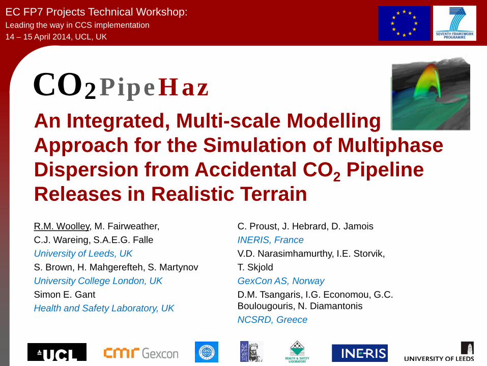
CO2PipeHaz An Integrated, Multi-scale Modelling Approach for the Simulation of Multiphase Dispersion from Accidental CO2 Pipeline Releases in Realistic Terrain R.M. Woolley, M. Fairweather, C.J. Wareing, S.A.E.G. Falle University of Leeds, UK S. Brown, H. Mahgerefteh, S. Martynov University College London, UK Simon E. Gant Health and Safety Laboratory, UK

EC FP7 Projects Technical Workshop: Leading the way in CCS implementation 14 – 15 April 2014, UCL, UK

C. Proust, J. Hebrard, D. Jamois INERIS, France V.D. Narasimhamurthy, I.E. Storvik, T. Skjold GexCon AS, Norway D.M. Tsangaris, I.G. Economou, G.C. Boulougouris, N. Diamantonis NCSRD, Greece

INERIS (France)

Prof. C. Proust

National Research Centre for Physical Sciences (Greece)

Prof. I. Economu, Dr. D. Tsangaris

University of Leeds (UK)

Prof. M. Fairweather

University College London, (UK) Prof. H. Mahgerefteh

Dalian University of Technology (China) Prof. Y. Zhang

GexCon AS (Norway) Dr. J.A. Melheim,

Health and Safety Laboratory (UK)

Dr. M. Wardman Dr. S. Gant

Project Partners

Outline Introduction – Work in context Experimental Configuration Realistic Industrial Release Case In-pipe and Release Condition Modelling Thermodynamic Property Modelling Near-field Multi-phase Dispersion Model Far-field Dispersion Model

Decision Support Tools Conclusions

Schematic of CO2 pipeline release and dispersion scenario

Introduction - Work in Context

Until P = Patm

Far-Field Near-field

Transfer of data between models

Integration of numerical models

Output from in-pipe modelling

Φ45°

E

Φ (mm) E (mm) e (mm)5.8 9 58.9 15 1011.8 15 1225 15 1050 No screw No screw

2 m3 vessel Connection to the discharge pipe End of the discharge pipe

General view discharge orifice

Experimental Configuration

Experimental Configuration

Mast No :1 2 3 4 5 6

Release point

2 m3 vessel

Masts : N°1 @ 1m N°2 @ 2m N°3 @ 5m N°4 @ 10m N°5 @ 20m N°6 @ 37m

0 +20 +30

+110

+140

+170

-20 -30 -40

-60

-130

-140

+40

+60

-10

+10

Release point is 1.5 m above ground

: Thermocouple K ± 0.25°C : O2 analyser ± 0.01% v/v

Experimental Configuration

Near-field instrumentation

Test Number Observed Mean Mass Flow

Rates / kg s-1

Ambient Temperature / K

Air Humidity / %

Reservoir Pressure /

bar

Nozzle Diameter / mm

11 7.7 276.15 >95 83 12 12 24.0 276.15 >95 77 25 13 40.0 276.65 >95 69 50

High-speed camera still of a 9mm release

R.M. Woolley, M. Fairweather, C.J. Wareing, S.A.E.G. Falle, C. Proust, J. Hebrard, D. Jamois, 2013, Experimental Measurement and Reynolds-Averaged Navier-Stokes Modelling of the Near-Field Structure of Multi-phase CO2 Jet Releases, Int. J. Greenh. Gas Con., 18, 1, 139-149.

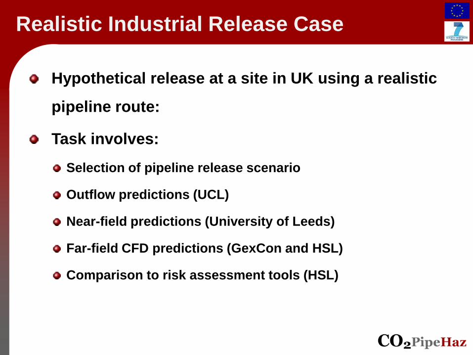
Hypothetical release at a site in UK using a realistic

pipeline route:

Task involves:

Selection of pipeline release scenario

Outflow predictions (UCL)

Near-field predictions (University of Leeds)

Far-field CFD predictions (GexCon and HSL)

Comparison to risk assessment tools (HSL)

Realistic Industrial Release Case

Pipe diameter 36” (ext. 914 mm, int. 870 mm) Wall thickness 22 mm Length 217 km Pressure 150 bar Temperature 10 ºC Composition 100% CO2

Failure mode Full-bore guillotine rupture Upstream flow No pump or reservoir Block valves None

0

100

200

300

400

500

600

0 50 100 150 200

Distance (km)

Pipe

line

Elev

atio

n (m

)

Elevation (m)Rupture Location

Pipeline outflow results found to be insensitive to terrain

Realistic Industrial Release Case

0

1

2

3

4

5

6

7

8

0 20 40 60 80

Crater Length (m)

Cra

ter D

epth

(m)

Historical Nat. GasAssumed CO2

Crater dimensions assumed, based on natural gas incident data

12 m

30 m

1 m

45º

4 m

Plan View Side View

12 m

0

5

10

15

20

25

30

35

0 20 40 60 80

Crater Length (m)

Cra

ter W

idth

(m)

Realistic Industrial Release Case

In-pipe and Release Condition Modelling

Tasks: To develop a multiphase heterogeneous outflow model for predicting CO2 discharge rate and fluid state during pipeline failure

Validate against large and small scale experimental data from INERIS and DUT

Method: 1D transient CFD

Finite Volume method Godunov 1st order scheme Harten, Lax, van Leer (HLL) solver Explicit time integration Model closure required for the thermo-physical properties of the phases (liquid, vapour and solid)

Brown, S., Martynov, S., Mahgerefteh,H., Proust, C., 2013. A Homogeneous Equilibrium Relaxation Flow Model for the Full Bore Rupture of Dense Phase CO2 Pipelines. Int. J. Greenh. Gas Con. 17, 349-356.

0.1

1.0

10.0

100.0

1000.0

10000.0

-100 -80 -60 -40 -20 0 20 40Temperature, °C

Pres

sure

, bar

SaturationMeltingSublimationPhastUCL

Solid

Liquid

Vapour

0

5,000

10,000

15,000

20,000

25,000

30,000

35,000

40,000

0 50 100 150 200

Time (s)

Tota

l mas

s re

leas

e ra

te (k

g/s)

UCLPhast

Starting Condition (150 bar, 10 ºC)

0

0.1

0.2

0.3

0.4

0.5

0.6

0.7

0.8

0.9

1

0 50 100 150 200

Time (s)

Liqu

id m

ass

frac

tion

(w/w

)

UCLPhast

UCLPhast

In-pipe and Release Condition Modelling

S. Brown, S. Martynov, H. Mahgerefteh, C. Proust, 2013, A Homogeneous Equilibrium Relaxation Flow Model for the Full Bore Rupture of Dense Phase CO2 Pipelines, Int. J. Greenh. Gas Con., 17, 349-356.

For CO2 and CO2 mixtures, the Physical Properties Library (PPL) developed by NCSRD can be used to obtain the following properties:

Volumetric (density, compressibility)

Energy related (enthalpy, entropy, heat capacity)

Derivative (Joule-Thomson, speed of sound)

Transport (viscosity, diffusivity, thermal conductivity)

and these properties can be obtained:

Cubic equations of state (Redlich-Kwong, Soave-Redlich-Kwong, Peng-Robinson, Peng-Robinson-Gasem, )

Specialized equations of state (GERG, Span and Wagner, Yokozeki)

Advanced equations of state (SAFT/PC-SAFT/tPC-PSAFT)

Thermodynamic Property Modelling

Thermodynamic Property Modelling

CO2 Speed of sound CO2 Joule-Thompson coefficient

Predictions of CO2 properties obtained using SAFT approach

N.I. Diamantonis, G.C. Boulougouris, E. Mansoor, D.M. Tsangaris, I.G. Economou, 2013, Evaluation of Cubic, SAFT, and PC-SAFT Equations of State for the Vapor-liquid Equilibrium Modeling of CO2 Mixtures with other Gases, Ind. Eng. Chem. Res., 52, 10, 3933-3942.

Near-field Multi-phase Dispersion Model

Conservative, upwind, finite volume code solving the Reynolds-averaged Navier-Stokes equations for mass, momentum, total energy, and mean of mixture fraction.

Adaptive Mesh Refinement with a hierarchy of grids – Solution computed on all grids. Mesh is then refined where solution varies rapidly.

For shock calculations - an HLL (Harten, Lax, van Leer) Riemann solver is used.

Coordinates: axisymmetric cylindrical polar or full three-dimensions.

Non-ideal Equation of State

Internal energy on the saturation line for the improved equation of state.

C.J. Wareing, R.M. Woolley, M. Fairweather, S.A.E.G. Falle, 2013, A Composite Equation of State for the Modelling of Sonic Carbon Dioxide Jets, AIChE J., 59, 10, 3928-3942.

Gas Phase: Peng-Robinson Eqn of State

Liquid Phase: Span & Wagner

Eqn of State Latent heat: DIPPR data

Solid phase: DIPPR data

Near-field Multi-phase Dispersion Model

Temperature Predictions of INERIS Releases - Liquid Release

Test 8x = 1md = 40

160

180

200

220

240

260

280

300

Tem

pera

ture

/ K

Test 6x = 1md = 112

Test 7x = 1md = 85

160

180

200

220

240

260

280

300

Tem

pera

ture

/ K

Test 6x = 2md = 225

Test 7x = 2md = 170

Test 8x = 2md = 80

Test 6 Pressure = 95 bar, diameter = 9 mm

Test 7 Pressure = 85 bar, diameter = 12 mm

Test 8 Pressure = 77 bar, diameter = 25 mm

-1.2 -0.8 -0.4 0.0 0.4 0.8 1.2

160

180

200

220

240

260

280

300

Tem

pera

ture

/ K

y / m

Test 6x = 5md = 562

-1.2 -0.8 -0.4 0.0 0.4 0.8 1.2y / m

Test 7x = 5md = 424

-1.2 -0.8 -0.4 0.0 0.4 0.8 1.2y / m

Test 8x = 5md = 200

Near-field Multi-phase Dispersion Model

X = 0.0

3-D crater geometry - 2 axisymmetric boundaries

Z = 0.0

Near-field Multi-phase Dispersion Model

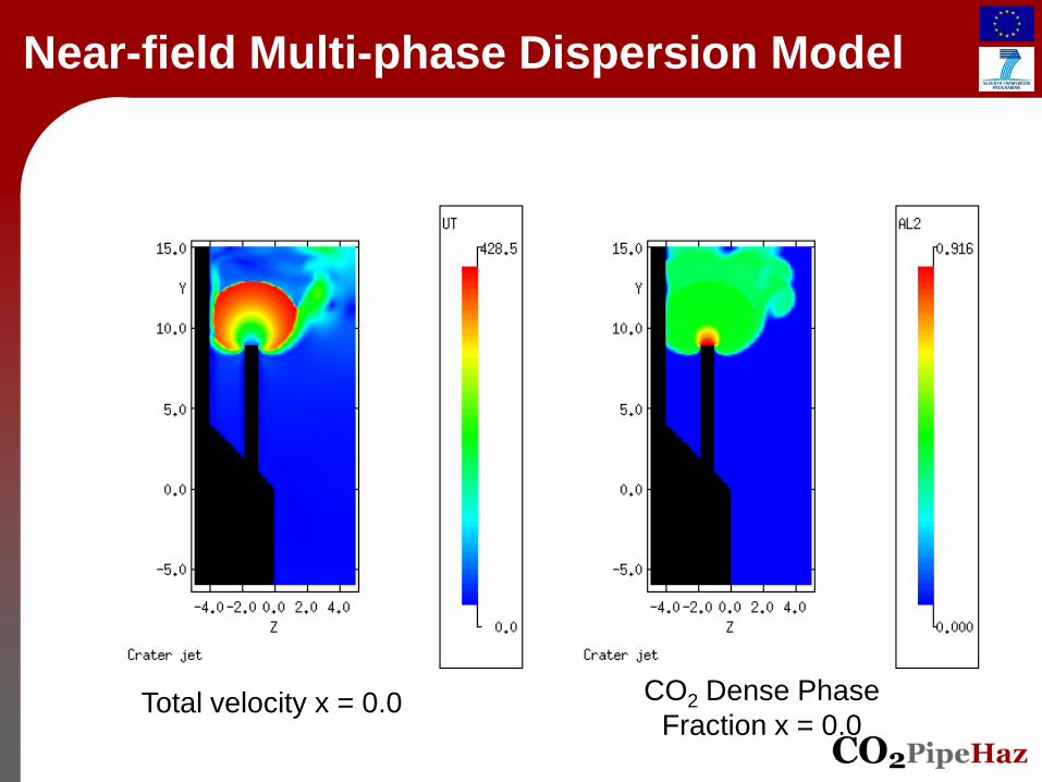
Near-field Multi-phase Dispersion Model

Total velocity x = 0.0 CO2 Dense Phase Fraction x = 0.0

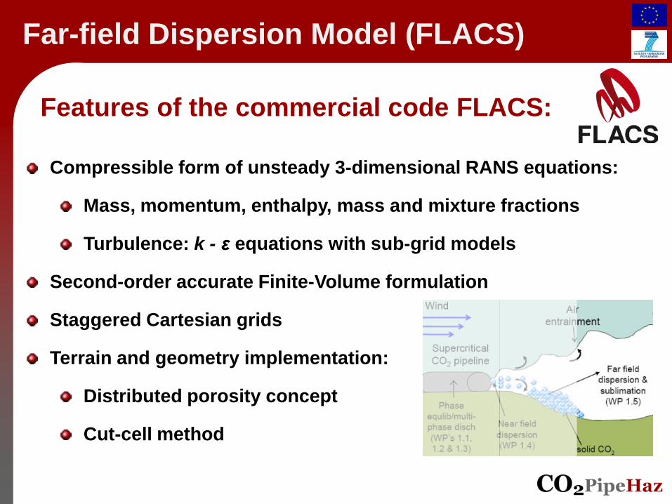
Far-field Dispersion Model (FLACS)

Compressible form of unsteady 3-dimensional RANS equations:

Mass, momentum, enthalpy, mass and mixture fractions

Turbulence: k - ε equations with sub-grid models

Second-order accurate Finite-Volume formulation

Staggered Cartesian grids

Terrain and geometry implementation:

Distributed porosity concept

Cut-cell method

Features of the commercial code FLACS:

Far-field Dispersion Model (FLACS) Multi-phase dispersion: Euler-Lagrange model

Non-compressible spherical particles: solids and droplets

Point-particle method (Loth, 2000)

Two-way coupling between the continuous phase (gas) and the dispersed phase (particles):

Source terms in the mass, momentum and energy equations

Particle-turbulence interaction: source terms in k - ε equations

Droplet vaporization and particle deposition on obstacles are modelled

Particle-particle interactions not considered.

Particle momentum equation: simplified Maxey and Riley’s equation

Buoyancy and drag forces are considered

Instantaneous fluid velocity seen by the particle: modeled by stochastic differential equations - modified Langevin equation

Far-field Dispersion Model (ANSYS-CFX) Lagrangian particle-tracking for solid CO2 particles

Sublimation: accounts for mass and heat transfer, and particle size reduction

Initial particle diameter assumed 20 μm

Humidity: Transported water vapour and dispersed water droplets

Numerics: Finite volume, high-order upwind-biased convection scheme, ~0.6M cells

Terrain data purchased from Ordnance Survey

3D far-field geometry imported into FLACS and CFX

Imported terrain in FLACS Imported terrain in CFX

Release location

10 km 5 km

Far-field Dispersion Model

Terrain imported in FLACS using CP-8 objects (which employs

porosity-concept rather than the cut-cell method).

A coarse grid of ≈ 350,000 was adopted for this test run.

Wind profile: 2 m/s, Pasquill class ‘D’, reference height 10 m and

ground-roughness 0.1 m

Release location

Wind direction

Sensors are placed 2m above the local ground

Far-field Dispersion Model

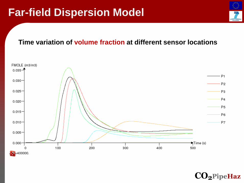
Time variation of volume fraction at different sensor locations

Far-field Dispersion Model

Far-field Dispersion Model

Predicted CO2 jet in the vicinity of the crater using FLACS (left) and CFX (right)

Far-field Dispersion Model

CFX predicted steady-state CO2 cloud, defined using three different mean CO2 concentrations: 1% v/v

(left); 2% v/v (middle); 4% v/v (right), and coloured according to the distance from the crater source.

28

TASKS:

Incorporate the predictive capabilities as described, as well as current knowledge and good practice, into decision support tools. Demonstrate the usefulness of tools to identify potential hazards by examining harm from vapour concentration and population density

Decision Support Tools

29

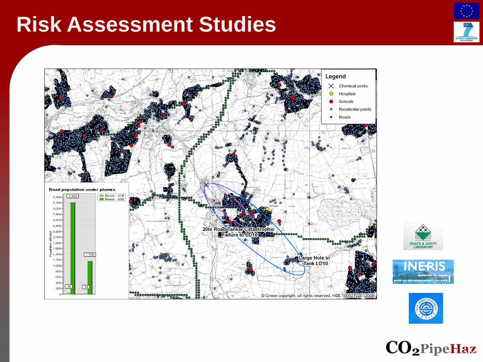
Risk Assessment Studies

• 1%, 10% and 50% fatality contours for indoor and outdoor populations weather condition and release point (standard TROD)

• figure shows 1% fatality contour for outdoor populations

• 72 wind directions (figure shows 4 directions)

• overlay with representative population data

Societal Risk Calculation

Conclusions

The process of simulating a hypothetical ‘realistic’ release from a buried 0.914 m (36 inch) diameter, 217 km long pipeline has been demonstrated. The work has demonstrated that it is feasible, in principle, to simulate such industrially-relevant flows. In view of the fact that most routine pipeline risk assessments will be carried out using integral or other phenomenological models that assume dispersion over flat terrain, it would be useful to use the models demonstrated here to determine under what set of conditions such models might provide unreliable results. Finally, from an emergency-planning perspective, it would be useful to further develop and validate models that are able to predict the extent of the visible CO2 plume, as well as its extent in terms of its instantaneous hazardous CO2 concentrations.

Acknowledgements & Disclaimer

The research leading to the results described in this presentation has received funding from the European Union 7th Framework Programme FP7-ENERGY-2009-1 under grant agreement number 241346. The presentation reflects only the authors’ views and the European Union is not liable for any use that may be made of the information contained therein.