Embed Size (px)
Citation preview
Wireless Personal Communications 5: 223–258, 1997.c 1997 Kluwer Academic Publishers. Printed in the Netherlands.
An Integrated Propagation-Mobility Interference Model forMicrocell Network Coverage Prediction
BRENDAN C. JONES and DAVID J. SKELLERNElectronics Department, School of Maths, Physics, Computing and Electronics, Macquarie University,NSW 2109 Australia. e-mail: [email protected], and daves@mpce. mq.edu.au
Abstract. This paper presents a new interference model for microcellular networks which integrates radio propa-gation parameters and user terminal mobility. This model uses a parameter denoted the “interference to noise ratio”(INR) to obtain a simplified description of mobile link outage contours as a function of the location of the fixedand mobile radio ports. The INR is used to demonstrate that microcell networks are more interference limited thanmacrocell networks, and thus are more affected by user terminal mobility. Expressions are derived for the INR anduser terminal cell radius distributions.
It is shown that in microcell systems a significant proportion of terminals may not be able to meet a contiguouscoverage criterion, and that closer microcell spacing can reduce rather than improve the coverage quality. Exami-nation of cochannel and adjacent channel reuse ratios in DCA microcell systems suggest that the closer frequencyreuse is primarily responsible for these coverage effects. Monte Carlo simulations are used to test the analyticaltheory. These results may form the basis of a design methodology for microcell systems.
Key words: Interference modelling, microceus, radio coverage.
1. Introduction
The concept of cellular telephony is largely attributable to developments in radiotelephonyat the Bell Telephone Laboratories from the late 1940s to the early 1970s [1, 2], and thesedevelopments led to the first commercial cellular telephone services being launched in theearly 1980s [2, 3]. Since that time, the growth and popularity of mobile telecommunicationshas been extraordinary.
The capacity of cellular systems can be increased by splitting and sectorising existingcells, thereby reusing frequencies more often in a geographic area. In practice, however, thereis a capacity limit as cells cannot be split indefinitely. The lower cell radius limit for mostconventional cellular systems (herein referred to as “macrocells”) is in the range of 1 to 1.5 km[4].
Microcell technologies are being developed to provide wireless communications to verylarge numbers of people at a much higher user density than is possible with macrocells [5].Microcell architecture differs from macrocell architecture in three fundamental ways:
� The cells are typically less than 1 km in radius.� The mobile terminals radiate at much lower power levels.� All radio channels are available in every cell.
The wide scale deployment of an extensive, high grade, wireless telephone system willrequire engineering tools and techniques that allow rapid and accurate system design [4, 6].The fundamental problem that needs to be addressed is modelling the end result of many userstransmitting in a congested area [6].
PREPROOFS: HANS: PIPS NO.: 120129 ENGIwiremh03.tex; 9/12/1997; 12:02; v.5; p.1
224 Brendan C. Jones and David J. Skellern
As the number of deployed microcells increases, site-by-site engineering may becometoo time consuming and costly. Yet service quality targets, including cell coverage and callblocking and dropping probabilities, will need to be able to be predicted and met. Thiswill require a design methodology that takes into account the competing requirements ofminimising the number of cell sites, minimising the system roll-out time, and minimising thesystem design cost.
It has been claimed that “a well founded radio network planning methodology does not yetexist” [7] and certainly there does not yet appear to be a systematic design methodology forengineering a microcell network to a target service quality [4–13]. Consideration of servicequality as part of the system design is an imperative because as the user base increases, peoplewill no longer accept poor call quality simply because the service is “mobile” [13] but willdemand a similar grade of service to that experienced in wireline services [4].
The applicability of macrocell design techniques to the microcell case is questionable.Firstly, macrocell systems use Fixed Channel Assignment (FCA) based upon an idealised,regular cell layout. This leads to a simple relationship between the “cluster size” C and thesignal to interference (S=I) performance of a receiver at a cell boundary in the presence ofcochannel interferers [14, 15]. However, no such simple relationship between cluster sizeand worst case S=I performance exists for microcells [16]. Microcell systems generally useDynamic Channel Assignment (DCA) and the cochannel reuse statistics are difficult to predict.
Secondly, assumptions that only the cochannel interferers dominate in a macrocell system[10] may not be applicable in microcell systems [17] as it has been shown that adjacent channelinterference (ACI) can affect the performance of heavily loaded cellular systems [18–20]. Inpractice, microcells often overlap and become irregular in shape [21], and the effects of ACIand further off-channel interference in microcells could be worse [17].
Thirdly, the close spacing of base stations in microcell systems (especially in multioperatorenvironments) and closer frequency reuse have a very significant impact upon the percentageof service area that has a circuit quality better than some specified value [5, 22, 23]. Althoughthe use of DCA and/or power control assists in controlling interference, these techniques canstill fail under heavy traffic loads [23, 24]. The impact of spatial traffic variability and userterminal mobility also needs to be considered [21, 22, 25].
The combination of these factors may make it very difficult to engineer a microcell systemso that reliable, contiguous radio coverage is achieved. Ubiquitous coverage may be impossibleto achieve [26, 27].
This paper presents a microcell interference model that enables analysis of microcellcoverage performance and could form the basis of a cell deployment methodology. Thefeatures of this model include:
� Uniform analysis of noise to interference limited environments.� Incorporation of the cumulative interference effects of all users.� Incorporation of terminal distribution models.
Both thermal noise and propagated interference are considered in the model because thetransmission quality is strongly dependent upon these two factors [28]. The interferenceeffects of all users are included in the model so as to avoid making assumptions about whichinterferers may dominate in the microcell environment.
Terminal distribution, hence mobility, is included in the model to avoid making assumptionsabout channel reuse distances. For example, Linnartz [29] assumed all interfering terminalsin an FCA system were located at the reuse distance; Wang and Rappaport [17, 18] assumed
wiremh03.tex; 9/12/1997; 12:02; v.5; p.2
An Integrated Propagation-Mobility Interference Model 225
terminals were in the “worst case” location in each cell; and Chuang [30] assumed terminalswere located at regular fixed points throughout the service area.
Other analyses, such as by Yao and Sheikh [31–34], Prasad and Kegel [35, 36] and Sowerbyand Williamson [37] avoid explicit terminal distributions by instead assuming interferers havecertain mean powers (the calculation of which is often left unstated), and that their powerenvelopes exhibit various statistics (e.g. Rice, Rayleigh, Nakagami, Suzuki) at the wantedreceiver. Otherwise, numerical analysis via a Monte Carlo simulation is performed, whereuponterminals are randomly placed in some fashion, e.g. Button [38, 39], Driscoll [19].
Of these analyses, only Sowerby and Williamson [37] have attempted to analyse in spatialterms the quality of radio coverage achieved by mobile terminals, rather than just computea blocking probability given the mean signal and interference powers at a receiver. Sowerbyand Williamson, however, did not express their results in terms of the probability of terminalsachieving an arbitrary cell radius, i.e. they did not calculate a cell radius distribution.
This paper demonstrates, in Section 2, the use of the microcell interference model indetermining spatial outage contours in the presence of interferers and shows how cell coverageis affected by the degree of interference domination of wanted links, extending the work ofSowerby and Williamson [37] and Cook [40].
Monte Carlo simulations are presented in Section 3 to demonstrate the effects of user densityand cell spacing on coverage in more complicated systems. In particular, the differences inthe INR and cell radius distributions between microcell and macrocell systems are examined,and it is investigated as to whether microcell coverage can be improved by adjusting the cellspacing.
In Section 4 a mathematical analysis (under simplifying assumptions) is presented whichillustrates how different terminal distribution models affect the INR and cell radius statistics.The results are compared with Monte Carlo simulations which do not make such simpli-fying assumptions. The cochannel and adjacent channel reuse statistics in DCA microcellsystems are compared with macrocell systems, and their impact upon microcell performanceis assessed. These results suggest that macrocell design principles cannot adequately predictmicrocell system performance and that the results obtained with the new model could formthe basis of a microcell design methodology.
2. A Microcell Interference Model
2.1. GENERAL NETWORK MODEL AND NOTATION
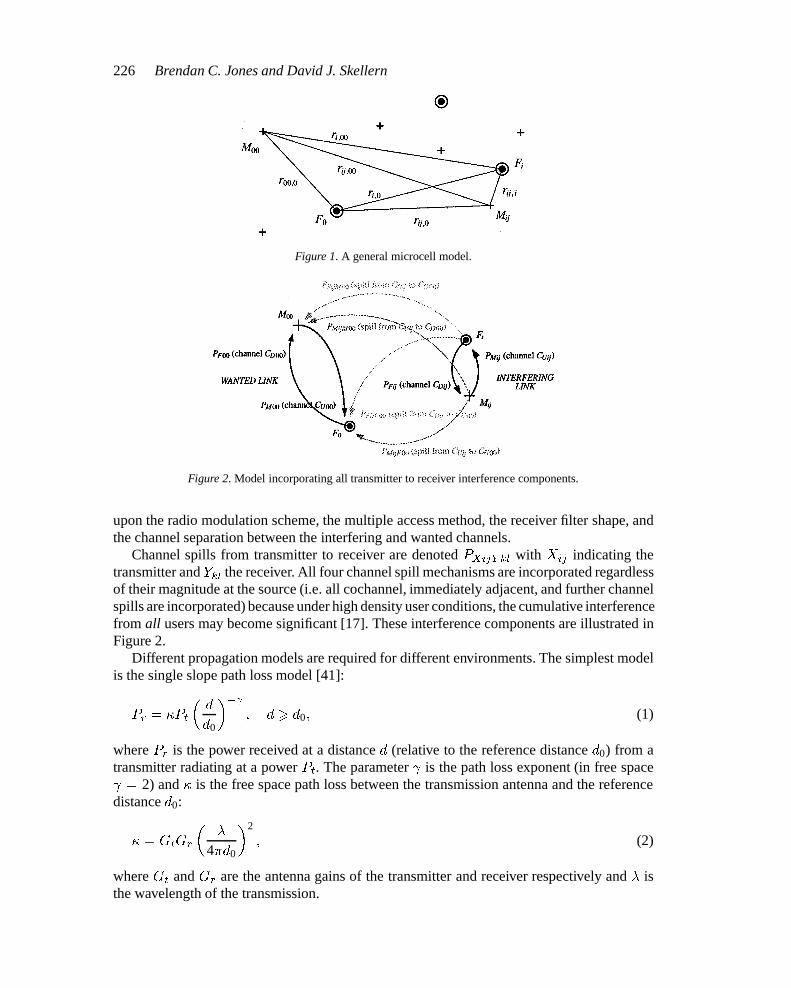
Consider the microcell network in Figure 1, consisting of a fixed station F0 and a mobilestation M00 attempting to establish a radio link in the presence of n additional fixed stationsFif1 6 i 6 ng. Each fixed station communicates with additional mobile stations Mijf1 6i 6 n; 1 6 j 6 mig, where mi is the total number of mobile stations communicating withfixed station Fi. The notation used for distances r between transmitters and receivers is asshown in Figure 1. Mobile terminalMij transmits to Fi at a power PMij on channelCUij (theuplink). Fixed station Fi transmits to mobile terminal Mij at a power PFij on channel CDij
(the downlink). The duplex channel Cij may comprise a pair of time-division duplex (TDD)slots within the one radio carrier, a pair of time-division multiple access (TDMA) slots acrossa pair of radio carriers, or a pair of frequency division multiple access (FDMA) carriers.
Each transmitter radiates power not only into its intended channel but into other channelsdue to finite transmitter filter roll-off. This is called channel spill, and its magnitude depends
wiremh03.tex; 9/12/1997; 12:02; v.5; p.3
226 Brendan C. Jones and David J. Skellern
Figure 1. A general microcell model.
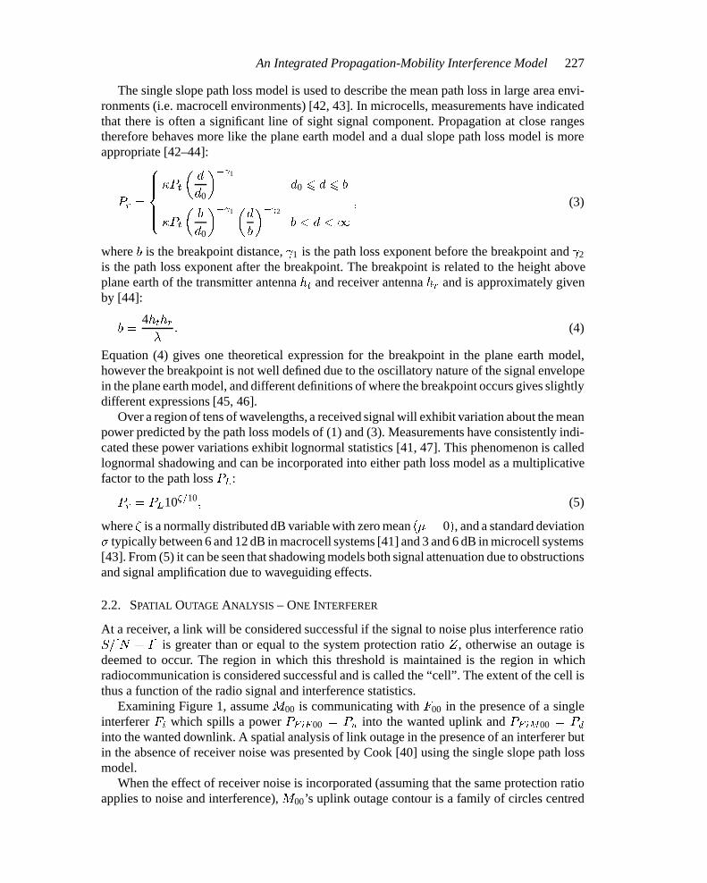
Figure 2. Model incorporating all transmitter to receiver interference components.
upon the radio modulation scheme, the multiple access method, the receiver filter shape, andthe channel separation between the interfering and wanted channels.
Channel spills from transmitter to receiver are denoted PXijY kl with Xij indicating thetransmitter and Ykl the receiver. All four channel spill mechanisms are incorporated regardlessof their magnitude at the source (i.e. all cochannel, immediately adjacent, and further channelspills are incorporated) because under high density user conditions, the cumulative interferencefrom all users may become significant [17]. These interference components are illustrated inFigure 2.
Different propagation models are required for different environments. The simplest modelis the single slope path loss model [41]:
Pr = �Pt
�d
d0
��
; d > d0; (1)
where Pr is the power received at a distance d (relative to the reference distance d0) from atransmitter radiating at a power Pt. The parameter is the path loss exponent (in free space = 2) and � is the free space path loss between the transmission antenna and the referencedistance d0:
� = GtGr
��
4�d0
�2
; (2)
where Gt and Gr are the antenna gains of the transmitter and receiver respectively and � isthe wavelength of the transmission.
wiremh03.tex; 9/12/1997; 12:02; v.5; p.4
An Integrated Propagation-Mobility Interference Model 227
The single slope path loss model is used to describe the mean path loss in large area envi-ronments (i.e. macrocell environments) [42, 43]. In microcells, measurements have indicatedthat there is often a significant line of sight signal component. Propagation at close rangestherefore behaves more like the plane earth model and a dual slope path loss model is moreappropriate [42–44]:
Pr =
8>>><>>>:�Pt
�d
d0
�� 1
d0 6 d 6 b
�Pt
�b
d0
�� 1
�d
b
�� 2
b < d <1; (3)
where b is the breakpoint distance, 1 is the path loss exponent before the breakpoint and 2
is the path loss exponent after the breakpoint. The breakpoint is related to the height aboveplane earth of the transmitter antenna ht and receiver antenna hr and is approximately givenby [44]:
b =4hthr�
: (4)
Equation (4) gives one theoretical expression for the breakpoint in the plane earth model,however the breakpoint is not well defined due to the oscillatory nature of the signal envelopein the plane earth model, and different definitions of where the breakpoint occurs gives slightlydifferent expressions [45, 46].
Over a region of tens of wavelengths, a received signal will exhibit variation about the meanpower predicted by the path loss models of (1) and (3). Measurements have consistently indi-cated these power variations exhibit lognormal statistics [41, 47]. This phenomenon is calledlognormal shadowing and can be incorporated into either path loss model as a multiplicativefactor to the path loss PL:
Pr = PL10�=10; (5)
where � is a normally distributed dB variable with zero mean (� = 0), and a standard deviation� typically between 6 and 12 dB in macrocell systems [41] and 3 and 6 dB in microcell systems[43]. From (5) it can be seen that shadowing models both signal attenuation due to obstructionsand signal amplification due to waveguiding effects.
2.2. SPATIAL OUTAGE ANALYSIS – ONE INTERFERER
At a receiver, a link will be considered successful if the signal to noise plus interference ratioS=[N + I] is greater than or equal to the system protection ratio Z , otherwise an outage isdeemed to occur. The region in which this threshold is maintained is the region in whichradiocommunication is considered successful and is called the “cell”. The extent of the cell isthus a function of the radio signal and interference statistics.
Examining Figure 1, assume M00 is communicating with F00 in the presence of a singleinterferer Fi which spills a power PFiF00 = Pu into the wanted uplink and PFiM00 = Pdinto the wanted downlink. A spatial analysis of link outage in the presence of an interferer butin the absence of receiver noise was presented by Cook [40] using the single slope path lossmodel.
When the effect of receiver noise is incorporated (assuming that the same protection ratioapplies to noise and interference), M00’s uplink outage contour is a family of circles centred
wiremh03.tex; 9/12/1997; 12:02; v.5; p.5
228 Brendan C. Jones and David J. Skellern
on the fixed station F0, but the downlink outage contour is a higher plane curve [48]. Byintroducing a parameter called the Interference to Noise Ratio (INR or �) the equations forboth outage contours can be written in a simple form. The INR is the total interference powerat a receiver divided by the receiver noise power. For a single interferer under the single slopepath loss model, the uplink INR (i.e. the INR at the fixed station F0) is given by [48]:
�u =�Pur
� i;0
N; (6)
while the downlink INR (at the mobile terminal M00) is given by:
�d =�Pdr
� i;00
N: (7)
Using this parameter, it can be shown that the equation for the uplink outage contour can bewritten [48]:
r 00;0(u) = Kur
i;0
��u
�u + 1
�=
�1
�u + 1
�(8)
and the downlink outage contour equation can be written:
r 00;0(d) = Kdr
i;00
��d
�d + 1
�=
�1
�d + 1
�; (9)
where = �Pt=ZN and the parameter K is given by [40]:
K =PtGtGrWiLs
ZPiWt; (10)
where Ls is a system loss factor, Pi is the interference power, and Wi and Wt are thebandwidths of the interfering and wanted signals respectively. If these bandwidths are equaland Gt, Gr and Ls are unity, the expression simplifies to Kd = Pt=ZPd for the downlinkand Ku = Pt=ZPu for the uplink. This parameter is a measure of the relative strength of theinterferer.
By using the INR as a parameter, these equations provide a seamless description of thesize and shape of the outage contours for all interference conditions from purely noise limitedto purely interference limited. In the noise only case (� = 0) the downlink and uplink outagecontours are circles centred on F0 of a radius determined by the receiver noise level. In theinterference only case (� !1) the equations reduce to those in [40].
As the receiver S=[N + I] threshold must be exceeded on both the uplink and downlinkin order for the duplex link to be successful, the range of the mobile terminal M00 from F0
in any direction is the minimum of ru and rd. Thus the range described by (8) represents themaximum possible range (i.e. cell radius) for M00 regardless of the downlink conditions.
2.3. OUTAGE CONTOURS – ONE INTERFERER
The downlink outage (9) can be rewritten in terms of �u using the relationship �d =�u(Pd=Pu)(ri;0=ri;00)
[48] giving:
r d = r
i;0[Kd � r
dPur
� i;0 =Pd�u]: (11)
wiremh03.tex; 9/12/1997; 12:02; v.5; p.6
An Integrated Propagation-Mobility Interference Model 229
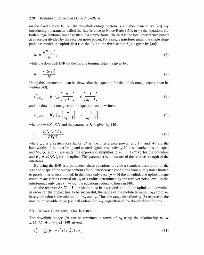
Figure 3. Outage contours for K = 0:1, = 2.
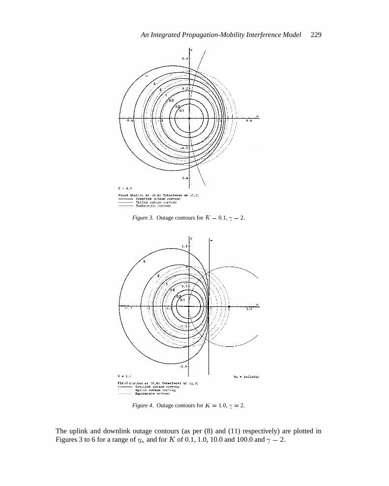
Figure 4. Outage contours for K = 1:0, = 2.
The uplink and downlink outage contours (as per (8) and (11) respectively) are plotted inFigures 3 to 6 for a range of �u and for K of 0.1, 1.0, 10.0 and 100.0 and = 2.
wiremh03.tex; 9/12/1997; 12:02; v.5; p.7
230 Brendan C. Jones and David J. Skellern
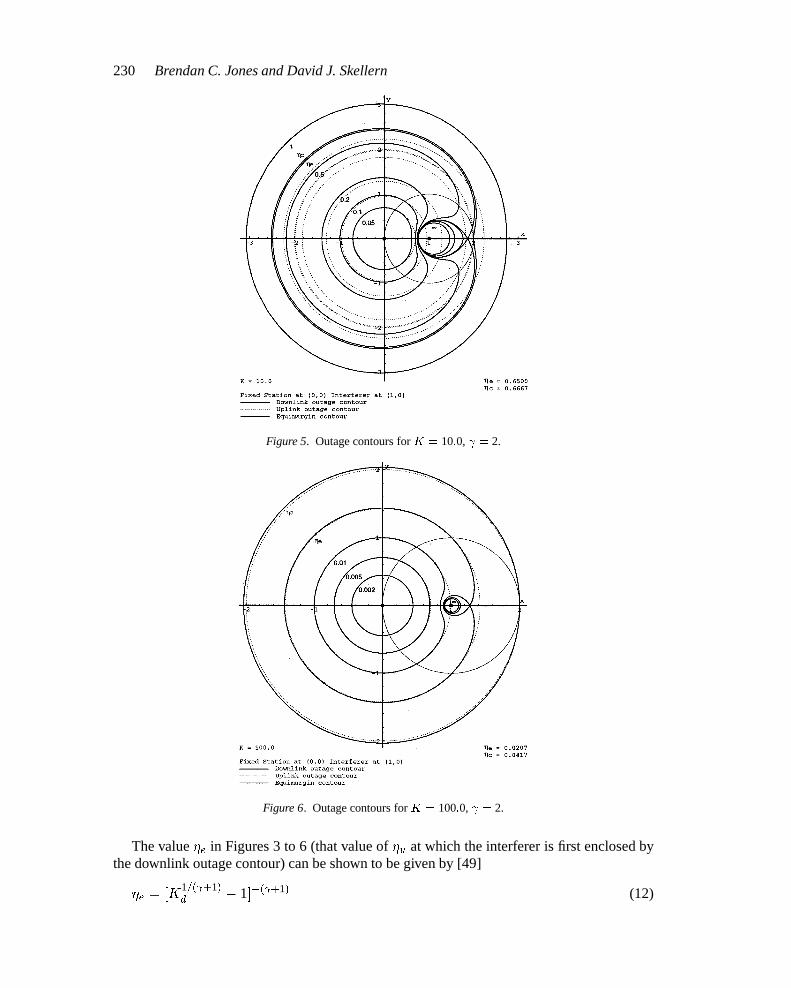
Figure 5. Outage contours for K = 10:0, = 2.
Figure 6. Outage contours for K = 100:0, = 2.
The value �e in Figures 3 to 6 (that value of �u at which the interferer is first enclosed bythe downlink outage contour) can be shown to be given by [49]
�e = [K1=( +1)d � 1]�( +1) (12)
wiremh03.tex; 9/12/1997; 12:02; v.5; p.8
An Integrated Propagation-Mobility Interference Model 231
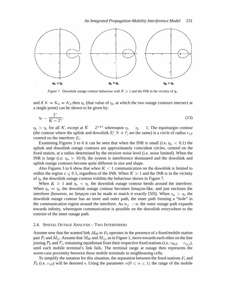
Figure 7. Downlink outage contour behaviour with K > 1 and the INR in the vicinity of �e.
and if K = Ku = Kd then �c (that value of �u at which the two outage contours intersect ata single point) can be shown to be given by:
�c =2
K � 2 ; (13)
�e > �c for all K , except at K = 2 +1 whereupon �c = �e = 1. The equimargin contour(the contour where the uplink and downlink S=[N + I] are the same) is a circle of radius ri;0centred on the interferer Fi.
Examining Figures 3 to 6 it can be seen that when the INR is small (i.e. �u < 0:1) theuplink and downlink outage contours are approximately coincident circles, centred on thefixed station, at a radius determined by the receiver noise level (i.e. noise limited). When theINR is large (i.e. �u > 10:0), the system is interference dominated and the downlink anduplink outage contours become quite different in size and shape.
Also Figures 3 to 6 show that when K < 1 communication on the downlink is limited towithin the region x 6 0:5, regardless of the INR. When K > 1 and the INR is in the vicinityof �e the downlink outage contour exhibits the behaviour shown in Figure 7.
When K > 1 and �u < �e the downlink outage contour bends around the interferer.When �u = �e the downlink outage contour becomes limacon-like, and just encloses theinterferer (however, no limacon can be made to match it exactly [50]). When �u > �e thedownlink outage contour has an inner and outer path, the inner path forming a “hole” inthe communication region around the interferer. As nu!1 the outer outage path expandstowards infinity, whereupon communication is possible on the downlink everywhere to theexterior of the inner outage path.
2.4. SPATIAL OUTAGE ANALYSIS – TWO INTERFERERS
Assume now that the wanted link M00 to F0 operates in the presence of a fixed/mobile stationpairFi andMij . Assume thatM00 andMij , as in Figure 1, move towards each other on the linejoining F0 and Fi, remaining equidistant from their respective fixed stations (i.e. r00;0 = rij;i),until each mobile terminal’s link fails. The terminal range at outage then represents theworst-case proximity between these mobile terminals in neighbouring cells.
To simplify the notation for this situation, the separation between the fixed stations Fi andF0 (i.e. ri;0) will be denoted s. Using the parameter �(0 6 � 6 1) the range of the mobile
wiremh03.tex; 9/12/1997; 12:02; v.5; p.9
232 Brendan C. Jones and David J. Skellern
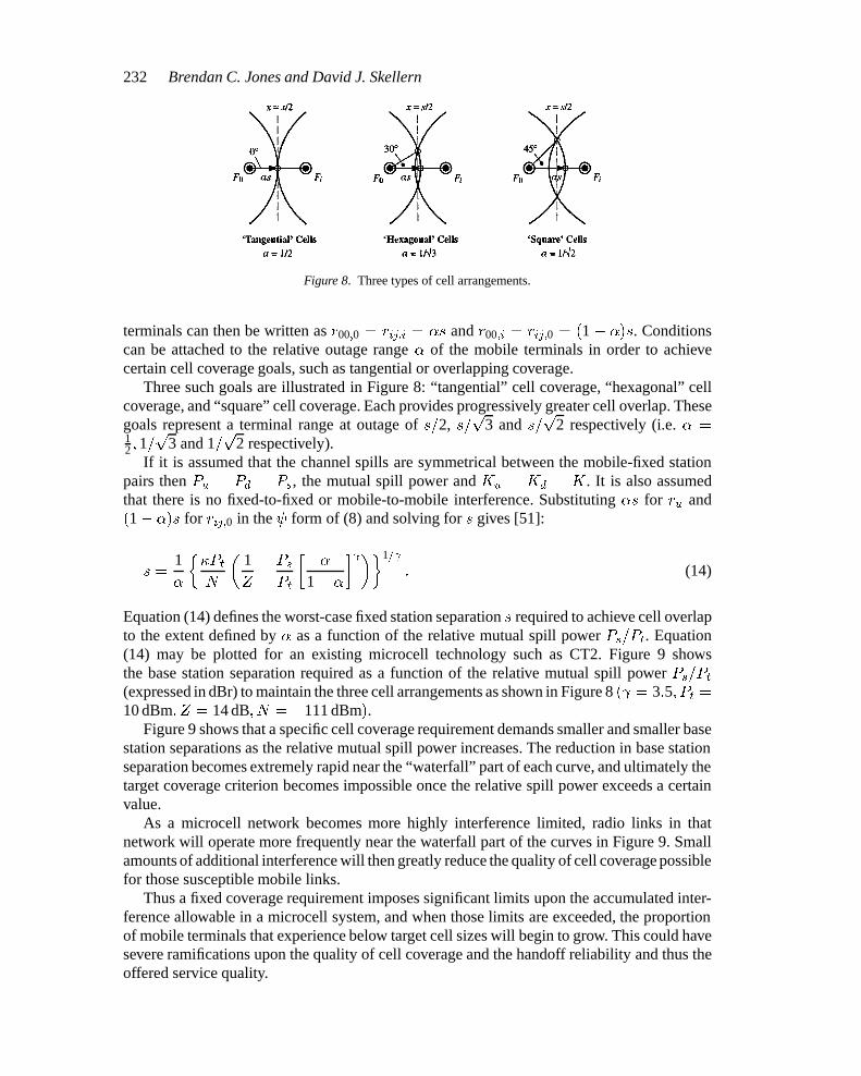
Figure 8. Three types of cell arrangements.
terminals can then be written as r00;0 = rij;i = �s and r00;i = rij;0 = (1 � �)s. Conditionscan be attached to the relative outage range � of the mobile terminals in order to achievecertain cell coverage goals, such as tangential or overlapping coverage.
Three such goals are illustrated in Figure 8: “tangential” cell coverage, “hexagonal” cellcoverage, and “square” cell coverage. Each provides progressively greater cell overlap. Thesegoals represent a terminal range at outage of s=2, s=
p3 and s=
p2 respectively (i.e. � =
12 ; 1=
p3 and 1=
p2 respectively).
If it is assumed that the channel spills are symmetrical between the mobile-fixed stationpairs then Pu = Pd = Ps, the mutual spill power and Ku = Kd = K . It is also assumedthat there is no fixed-to-fixed or mobile-to-mobile interference. Substituting �s for ru and(1� �)s for rij;0 in the form of (8) and solving for s gives [51]:
s =1�
��Pt
N
�1Z� Ps
Pt
��
1� �
� ��1=
: (14)
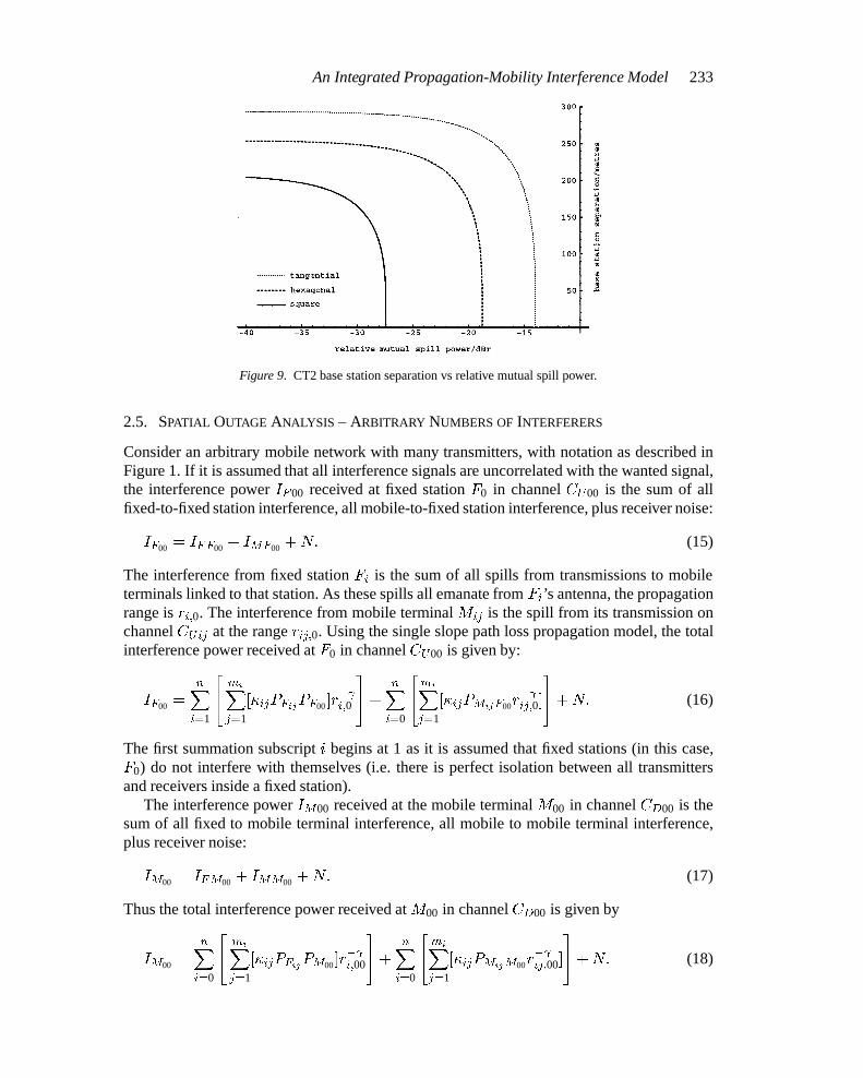
Equation (14) defines the worst-case fixed station separation s required to achieve cell overlapto the extent defined by � as a function of the relative mutual spill power Ps=Pt. Equation(14) may be plotted for an existing microcell technology such as CT2. Figure 9 showsthe base station separation required as a function of the relative mutual spill power Ps=Pt(expressed in dBr) to maintain the three cell arrangements as shown in Figure 8 ( = 3:5; Pt =10 dBm; Z = 14 dB; N = �111 dBm).
Figure 9 shows that a specific cell coverage requirement demands smaller and smaller basestation separations as the relative mutual spill power increases. The reduction in base stationseparation becomes extremely rapid near the “waterfall” part of each curve, and ultimately thetarget coverage criterion becomes impossible once the relative spill power exceeds a certainvalue.
As a microcell network becomes more highly interference limited, radio links in thatnetwork will operate more frequently near the waterfall part of the curves in Figure 9. Smallamounts of additional interference will then greatly reduce the quality of cell coverage possiblefor those susceptible mobile links.
Thus a fixed coverage requirement imposes significant limits upon the accumulated inter-ference allowable in a microcell system, and when those limits are exceeded, the proportionof mobile terminals that experience below target cell sizes will begin to grow. This could havesevere ramifications upon the quality of cell coverage and the handoff reliability and thus theoffered service quality.
wiremh03.tex; 9/12/1997; 12:02; v.5; p.10
An Integrated Propagation-Mobility Interference Model 233
Figure 9. CT2 base station separation vs relative mutual spill power.
2.5. SPATIAL OUTAGE ANALYSIS – ARBITRARY NUMBERS OF INTERFERERS
Consider an arbitrary mobile network with many transmitters, with notation as described inFigure 1. If it is assumed that all interference signals are uncorrelated with the wanted signal,the interference power IF00 received at fixed station F0 in channel CU00 is the sum of allfixed-to-fixed station interference, all mobile-to-fixed station interference, plus receiver noise:
IF00 = IFF00 + IMF00 +N: (15)
The interference from fixed station Fi is the sum of all spills from transmissions to mobileterminals linked to that station. As these spills all emanate from Fi’s antenna, the propagationrange is ri;0. The interference from mobile terminal Mij is the spill from its transmission onchannel CUij at the range rij;0. Using the single slope path loss propagation model, the totalinterference power received at F0 in channel CU00 is given by:
IF00 =nXi=1
24 miXj=1
[�ijPFijPF00 ]r� i;0
35+ nX
i=0
24miXj=1
[�ijPMijF00r� ij;0]
35+N: (16)
The first summation subscript i begins at 1 as it is assumed that fixed stations (in this case,F0) do not interfere with themselves (i.e. there is perfect isolation between all transmittersand receivers inside a fixed station).
The interference power IM00 received at the mobile terminal M00 in channel CD00 is thesum of all fixed to mobile terminal interference, all mobile to mobile terminal interference,plus receiver noise:
IM00 = IFM00 + IMM00 +N: (17)
Thus the total interference power received at M00 in channel CD00 is given by
IM00 =nXi=0
24 miXj=1
[�ijPFijPM00 ]r� i;00
35+ nX
i=0
24miXj=1
[�ijPMijM00r� ij;00]
35+N: (18)
wiremh03.tex; 9/12/1997; 12:02; v.5; p.11
234 Brendan C. Jones and David J. Skellern
Hence, the general forms of the INR become [49, 52]:
�u00 =IFF00 + IMF00
N
=1N
8<:
nXi=1
24miXj=1
[�ijPFijF00 ]r� i;0
35+ nX
i=0
24miXj=1
[�ijPMijF00r� ij;0]
359=; ; (19)
�d00 =IFM00 + IMM00
N
=1N
8<:
nXi=0
24miXj=1
[�ijPFijM00 ]r� i;00
35+ nX
i=0
24miXj=1
[�ijPMijM00r� ij;00]
359=; : (20)
The outage contour expressions written in terms of the INR ((8) and (9)) still apply for thegeneral uplink and downlink INR expressions [49].
The mobile to mobile or fixed station to fixed station interference can be very small. Forexample, if a TDD/TDMA system is assumed to be perfectly synchronised then allPFijF00 andPMijM00 terms will be zero. Further, thePMijF00 andPFijM00 terms will be zero between anytwo transmitters using different timeslots. If however, a TDD/TDMA system is not perfectlysynchronised, then all interference terms could become significant.
In an FDMA system, the magnitude of the PFijF 00 and PMijM00 terms depends upon thepaired channel spill, i.e. how much RF radiation is spilled across the guard band used betweenthe uplink/downlink channel pair. This spill value may be very small but it is usually not zero.
Equations (19) and (20) may be used to spatially determine where outage would occur ifa mobile terminal (e.g. M00) moved around the cellular service area, i.e. determine the extentof M00’s cell. While (19) and (20) incorporate the impact of other interferers upon M00 as itmoves within the service area, they do not considerM00’s effect upon other receivers. If M00
moves close to another receiverMkl, it may spill sufficient additional interference into Mkl’sreceiver to cause an outage to Mkl but not to itself. Expressions for the regions in which thisoccurs were presented in [49].
3. Monte Carlo Simulation of Macrocell and Microcell Systems
3.1. SIMULATION METHODOLOGY
A computer program has been developed to model arbitrary cellular networks [49, 52]. Theprogram can generate “snapshot” cell coverage plots or perform Monte Carlo simulations toestimate call blocking and dropout statistics, and INR and cell radius densities and distribu-tions.
In each simulation, a random sequence of call attempts can be made from static mobileterminals randomly placed according to one of three distribution models. A mobile terminal’scall attempt is deemed to fail if it doesn’t meet the required S=[N + I] on both the uplinkand downlink. An initially successful mobile terminal can also drop out if the success of otherterminals leads to an increase in interference, causing its S=[N + I] to fall below threshold.In-cell channel reassignments and retries are permitted for DCA systems.
A “snapshot” cell plot comparison between a GSM system and a CT2 system was presentedin [49] which suggested that microcells exhibit a larger degree of cell radius variation than
wiremh03.tex; 9/12/1997; 12:02; v.5; p.12
An Integrated Propagation-Mobility Interference Model 235
macrocells due to greater interference domination of wanted links. In [52] Monte Carlosimulations were performed to compare the INR and cell radius statistics of various macrocelland microcell technologies. These results showed microcell networks exhibiting larger INRs(around a factor of 100) and larger cell radius spread (around a factor of 10) than macrocellnetworks.
These simulations were based upon a single slope path loss propagation model and signalshadowing. The effects of using a dual slope model in the microcell case, and signal shadowingin all cases, are now examined.
3.2. MACROCELL AND MICROCELL INR AND CELL RADIUS STATISTICS
The Monte Carlo simulation was loaded with the physical layer, call set up and channelallocation specifications for macrocell (AMPS and GSM) and microcell (CT2, DECT andPHS) technologies.
The number of simultaneous users per cell was adjusted in each system to achieve acomparable channel loading between the systems (10% of each cell’s available channels).Cells were deployed in a regular hexagonal pattern of one central cluster of cells and one tierof surrounding clusters, at a spacing commensurate with high density deployment of the giventechnology. Table 1 summarises the simulation parameters used. A cluster size of unity meansthat all RF channels are available in every cell.
A single slope path loss model was used for macrocell environments and the dual slopemodel was used for microcell environments (as explained in Section 2.1). The path lossexponents and shadowing deviation values are representative values taken from measurementsat appropriate frequencies and environments, reported by Marsan et al. [53], Seidel andRappaport [54], Xia et al. [44, 43], and Feuerstein et al. [42]. The breakpoint in the dual slopepath loss model assumed a lamp-post transmitter height of 6 m and a portable receiver athuman ear height of 1.5 m.
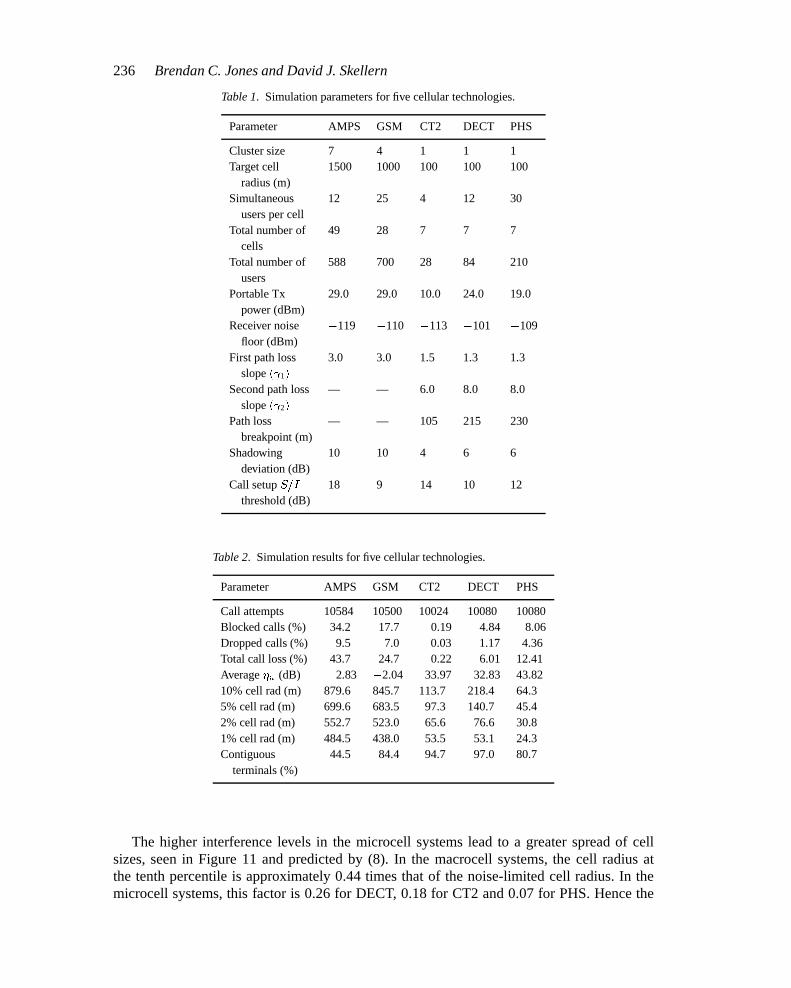
In each simulation, approximately 10000 static call attempts were made. For DECT, CT2and PHS, DCA was implemented in accordance with their specifications. Table 2 summarisesthe call failure statistics, including the rate of blocked and dropped calls. The average uplinkINR (�u) and standard deviation are also given for the successful terminals on a dB basis.
Finally, cell radius percentiles from the cell radius CDF are listed. For example, a “10%cell radius” of 100 m would indicate that 10% of successful terminals achieve a maximumcell radius of 100 m due to interference. Finally, the percentage of successful terminals whichcould maintain their link out to the target cell radius is given as “Contiguous Terminals (%)”.
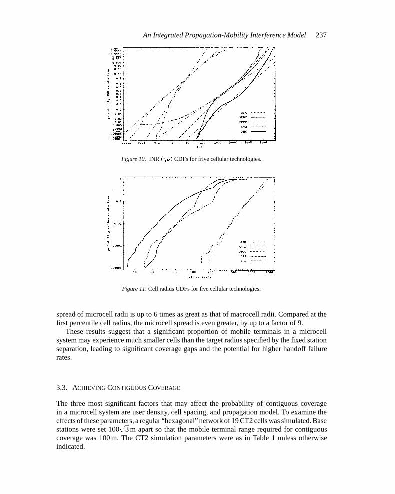
Table 2 shows the microcell systems modelled are significantly more interference limited(i.e. higher average �u) than the macrocell systems by a factor of 30 to 40 dB. Under the dualslope path loss model, most microcell interferers lie within range of the path loss breakpoint.As the initial path loss is small, the interference effects are worse than that seen with the singleslope, no shadowing model in [52]. Figure 10 plots the uplink INR (�u) CDF on a lognormalscale for each technology, and the difference in the INR distributions between microcell andmacrocell technologies is clear. The dashed lines represent the lognormal lines of best fit toeach data.
Figure 11 shows the cell radius CDF computed from the INR CDF using (8) and theappropriate path loss model. The path loss breakpoints in the microcell model appears as akink in the CDF traces for the microcell systems.
wiremh03.tex; 9/12/1997; 12:02; v.5; p.13
236 Brendan C. Jones and David J. Skellern
Table 1. Simulation parameters for five cellular technologies.
Parameter AMPS GSM CT2 DECT PHS
Cluster size 7 4 1 1 1Target cell 1500 1000 100 100 100
radius (m)Simultaneous 12 25 4 12 30
users per cellTotal number of 49 28 7 7 7
cellsTotal number of 588 700 28 84 210
usersPortable Tx 29.0 29.0 10.0 24.0 19.0
power (dBm)Receiver noise �119 �110 �113 �101 �109
floor (dBm)First path loss 3.0 3.0 1.5 1.3 1.3
slope ( 1)
Second path loss — — 6.0 8.0 8.0slope ( 2)
Path loss — — 105 215 230breakpoint (m)
Shadowing 10 10 4 6 6deviation (dB)
Call setup S=I 18 9 14 10 12threshold (dB)
Table 2. Simulation results for five cellular technologies.
Parameter AMPS GSM CT2 DECT PHS
Call attempts 10584 10500 10024 10080 10080Blocked calls (%) 34.2 17.7 0.19 4.84 8.06Dropped calls (%) 9.5 7.0 0.03 1.17 4.36Total call loss (%) 43.7 24.7 0.22 6.01 12.41Average �u (dB) 2.83 �2.04 33.97 32.83 43.8210% cell rad (m) 879.6 845.7 113.7 218.4 64.35% cell rad (m) 699.6 683.5 97.3 140.7 45.42% cell rad (m) 552.7 523.0 65.6 76.6 30.81% cell rad (m) 484.5 438.0 53.5 53.1 24.3Contiguous 44.5 84.4 94.7 97.0 80.7
terminals (%)
The higher interference levels in the microcell systems lead to a greater spread of cellsizes, seen in Figure 11 and predicted by (8). In the macrocell systems, the cell radius atthe tenth percentile is approximately 0.44 times that of the noise-limited cell radius. In themicrocell systems, this factor is 0.26 for DECT, 0.18 for CT2 and 0.07 for PHS. Hence the
wiremh03.tex; 9/12/1997; 12:02; v.5; p.14
An Integrated Propagation-Mobility Interference Model 237
Figure 10. INR (�F ) CDFs for frive cellular technologies.
Figure 11. Cell radius CDFs for five cellular technologies.
spread of microcell radii is up to 6 times as great as that of macrocell radii. Compared at thefirst percentile cell radius, the microcell spread is even greater, by up to a factor of 9.
These results suggest that a significant proportion of mobile terminals in a microcellsystem may experience much smaller cells than the target radius specified by the fixed stationseparation, leading to significant coverage gaps and the potential for higher handoff failurerates.
3.3. ACHIEVING CONTIGUOUS COVERAGE
The three most significant factors that may affect the probability of contiguous coveragein a microcell system are user density, cell spacing, and propagation model. To examine theeffects of these parameters, a regular “hexagonal” network of 19 CT2 cells was simulated. Basestations were set 100
p3 m apart so that the mobile terminal range required for contiguous
coverage was 100 m. The CT2 simulation parameters were as in Table 1 unless otherwiseindicated.
wiremh03.tex; 9/12/1997; 12:02; v.5; p.15
238 Brendan C. Jones and David J. Skellern
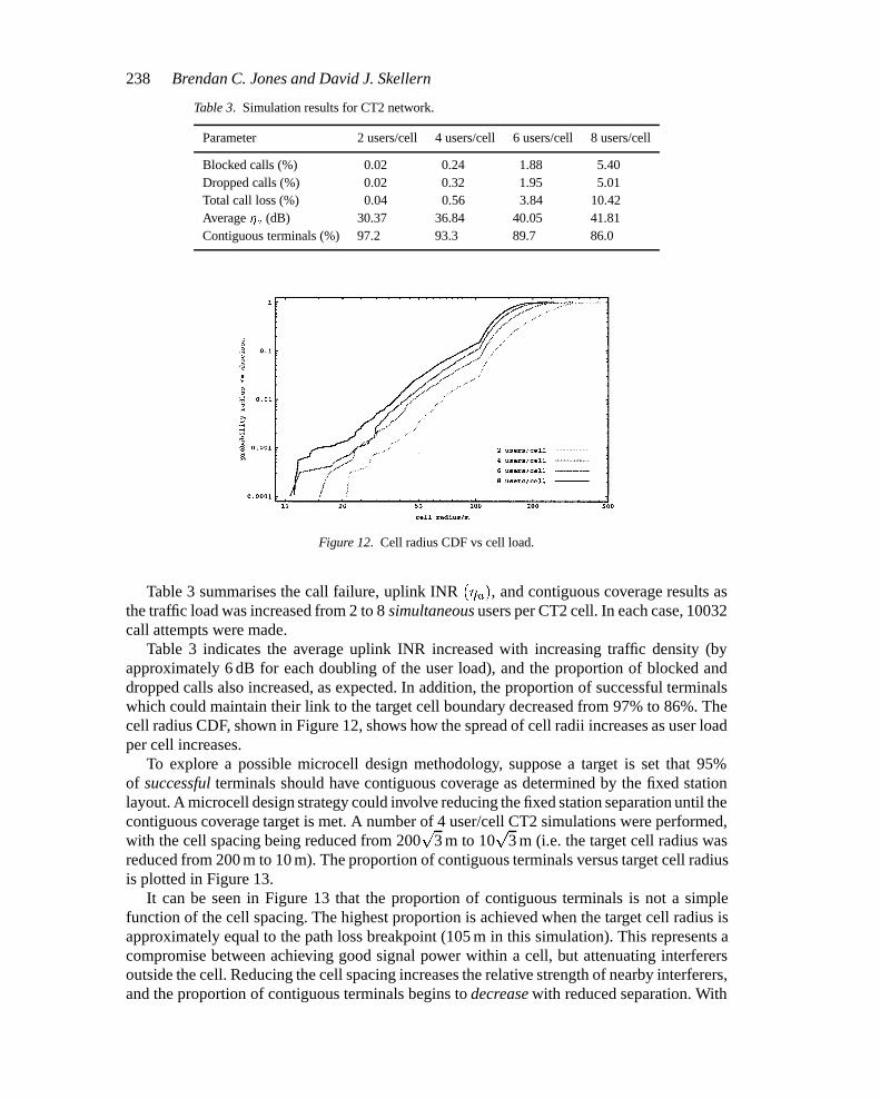
Table 3. Simulation results for CT2 network.
Parameter 2 users/cell 4 users/cell 6 users/cell 8 users/cell
Blocked calls (%) 0.02 0.24 1.88 5.40Dropped calls (%) 0.02 0.32 1.95 5.01Total call loss (%) 0.04 0.56 3.84 10.42Average �u (dB) 30.37 36.84 40.05 41.81Contiguous terminals (%) 97.2 93.3 89.7 86.0
Figure 12. Cell radius CDF vs cell load.
Table 3 summarises the call failure, uplink INR (�u), and contiguous coverage results asthe traffic load was increased from 2 to 8 simultaneous users per CT2 cell. In each case, 10032call attempts were made.
Table 3 indicates the average uplink INR increased with increasing traffic density (byapproximately 6 dB for each doubling of the user load), and the proportion of blocked anddropped calls also increased, as expected. In addition, the proportion of successful terminalswhich could maintain their link to the target cell boundary decreased from 97% to 86%. Thecell radius CDF, shown in Figure 12, shows how the spread of cell radii increases as user loadper cell increases.
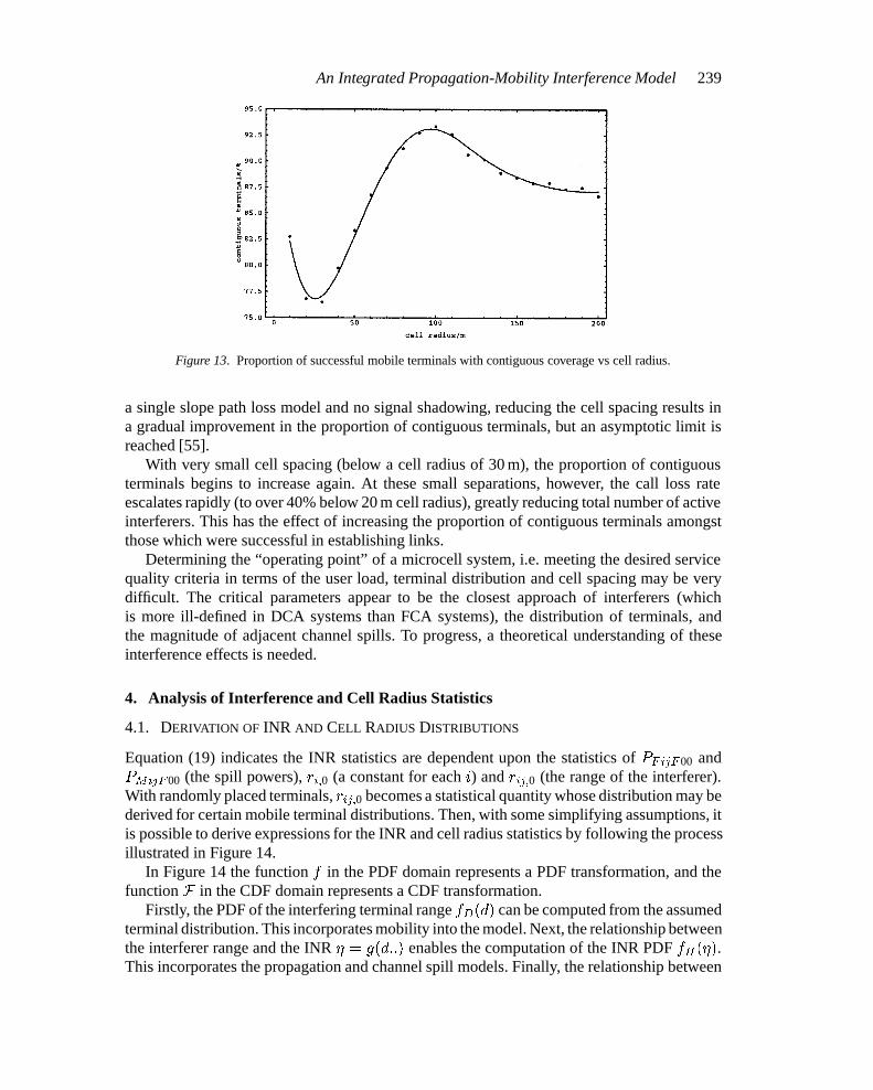
To explore a possible microcell design methodology, suppose a target is set that 95%of successful terminals should have contiguous coverage as determined by the fixed stationlayout. A microcell design strategy could involve reducing the fixed station separation until thecontiguous coverage target is met. A number of 4 user/cell CT2 simulations were performed,with the cell spacing being reduced from 200
p3 m to 10
p3 m (i.e. the target cell radius was
reduced from 200 m to 10 m). The proportion of contiguous terminals versus target cell radiusis plotted in Figure 13.
It can be seen in Figure 13 that the proportion of contiguous terminals is not a simplefunction of the cell spacing. The highest proportion is achieved when the target cell radius isapproximately equal to the path loss breakpoint (105 m in this simulation). This represents acompromise between achieving good signal power within a cell, but attenuating interferersoutside the cell. Reducing the cell spacing increases the relative strength of nearby interferers,and the proportion of contiguous terminals begins to decrease with reduced separation. With
wiremh03.tex; 9/12/1997; 12:02; v.5; p.16
An Integrated Propagation-Mobility Interference Model 239
Figure 13. Proportion of successful mobile terminals with contiguous coverage vs cell radius.
a single slope path loss model and no signal shadowing, reducing the cell spacing results ina gradual improvement in the proportion of contiguous terminals, but an asymptotic limit isreached [55].
With very small cell spacing (below a cell radius of 30 m), the proportion of contiguousterminals begins to increase again. At these small separations, however, the call loss rateescalates rapidly (to over 40% below 20 m cell radius), greatly reducing total number of activeinterferers. This has the effect of increasing the proportion of contiguous terminals amongstthose which were successful in establishing links.
Determining the “operating point” of a microcell system, i.e. meeting the desired servicequality criteria in terms of the user load, terminal distribution and cell spacing may be verydifficult. The critical parameters appear to be the closest approach of interferers (whichis more ill-defined in DCA systems than FCA systems), the distribution of terminals, andthe magnitude of adjacent channel spills. To progress, a theoretical understanding of theseinterference effects is needed.
4. Analysis of Interference and Cell Radius Statistics
4.1. DERIVATION OF INR AND CELL RADIUS DISTRIBUTIONS
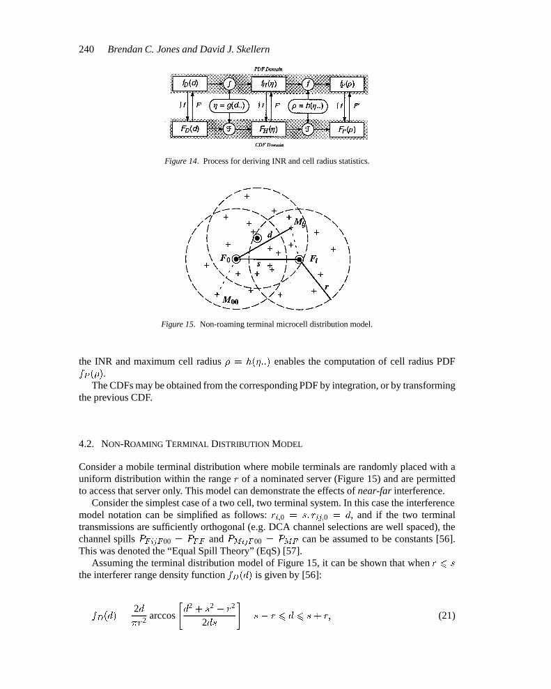
Equation (19) indicates the INR statistics are dependent upon the statistics of PFijF00 andPMijF00 (the spill powers), ri;0 (a constant for each i) and rij;0 (the range of the interferer).With randomly placed terminals, rij;0 becomes a statistical quantity whose distribution may bederived for certain mobile terminal distributions. Then, with some simplifying assumptions, itis possible to derive expressions for the INR and cell radius statistics by following the processillustrated in Figure 14.
In Figure 14 the function f in the PDF domain represents a PDF transformation, and thefunction F in the CDF domain represents a CDF transformation.
Firstly, the PDF of the interfering terminal range fD(d) can be computed from the assumedterminal distribution. This incorporates mobility into the model. Next, the relationship betweenthe interferer range and the INR � = g(d::) enables the computation of the INR PDF fH(�).This incorporates the propagation and channel spill models. Finally, the relationship between
wiremh03.tex; 9/12/1997; 12:02; v.5; p.17
240 Brendan C. Jones and David J. Skellern
Figure 14. Process for deriving INR and cell radius statistics.
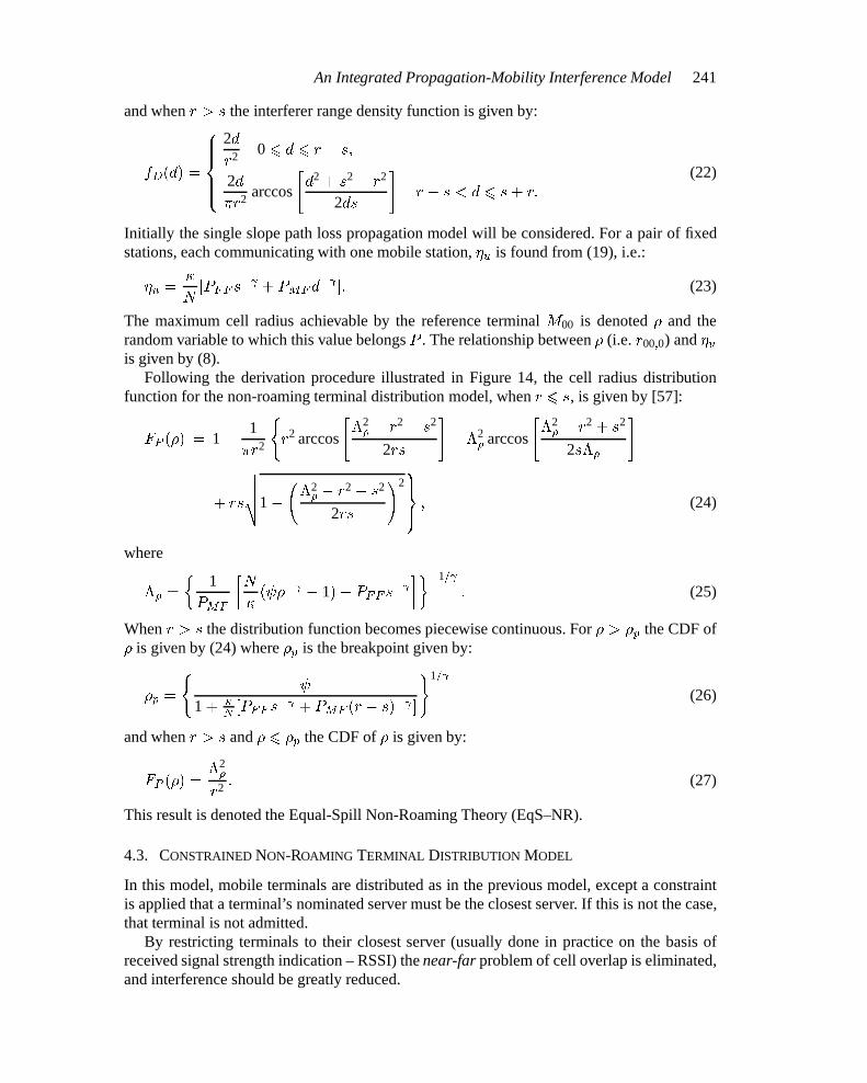
Figure 15. Non-roaming terminal microcell distribution model.
the INR and maximum cell radius � = h(�::) enables the computation of cell radius PDFfP (�).
The CDFs may be obtained from the corresponding PDF by integration, or by transformingthe previous CDF.
4.2. NON-ROAMING TERMINAL DISTRIBUTION MODEL
Consider a mobile terminal distribution where mobile terminals are randomly placed with auniform distribution within the range r of a nominated server (Figure 15) and are permittedto access that server only. This model can demonstrate the effects of near-far interference.
Consider the simplest case of a two cell, two terminal system. In this case the interferencemodel notation can be simplified as follows: ri;0 = s; rij;0 = d, and if the two terminaltransmissions are sufficiently orthogonal (e.g. DCA channel selections are well spaced), thechannel spills PFijF00 = PFF and PMijF00 = PMF can be assumed to be constants [56].This was denoted the “Equal Spill Theory” (EqS) [57].
Assuming the terminal distribution model of Figure 15, it can be shown that when r 6 sthe interferer range density function fD(d) is given by [56]:
fD(d) =2d�r2 arccos
"d2 + s2 � r2
2ds
#s� r 6 d 6 s+ r; (21)
wiremh03.tex; 9/12/1997; 12:02; v.5; p.18
An Integrated Propagation-Mobility Interference Model 241
and when r > s the interferer range density function is given by:
fD(d) =
8>>><>>>:
2dr2 0 6 d 6 r � s;
2d�r2 arccos
"d2 + s2 � r2
2ds
#r � s < d 6 s+ r:
(22)
Initially the single slope path loss propagation model will be considered. For a pair of fixedstations, each communicating with one mobile station, �u is found from (19), i.e.:
�u =�
N[PFF s
� + PMFd� ]: (23)
The maximum cell radius achievable by the reference terminal M00 is denoted � and therandom variable to which this value belongs P . The relationship between � (i.e. r00;0) and �uis given by (8).
Following the derivation procedure illustrated in Figure 14, the cell radius distributionfunction for the non-roaming terminal distribution model, when r 6 s, is given by [57]:
FP (�) = 1� 1�r2
(r2 arccos
"�2� � r2 � s2
2rs
#� �2
� arccos
"�2� � r2 + s2
2s��
#
+ rs
vuut1� �2� � r2 � s2
2rs
!29>=>; ; (24)
where
�� =
�1
PMF
�N
�( �� � 1)� PFF s
�
���1=
: (25)
When r > s the distribution function becomes piecewise continuous. For � > �p the CDF of� is given by (24) where �p is the breakpoint given by:
�p =
(
1 + �N [PFF s� + PMF (r � s)� ]
)1=
(26)
and when r > s and � 6 �p the CDF of � is given by:
FP (�) =�2�
r2 : (27)
This result is denoted the Equal-Spill Non-Roaming Theory (EqS–NR).
4.3. CONSTRAINED NON-ROAMING TERMINAL DISTRIBUTION MODEL
In this model, mobile terminals are distributed as in the previous model, except a constraintis applied that a terminal’s nominated server must be the closest server. If this is not the case,that terminal is not admitted.
By restricting terminals to their closest server (usually done in practice on the basis ofreceived signal strength indication – RSSI) the near-far problem of cell overlap is eliminated,and interference should be greatly reduced.
wiremh03.tex; 9/12/1997; 12:02; v.5; p.19
242 Brendan C. Jones and David J. Skellern
Figure 16. Roaming terminal microcell distribution model.
Consider again the two cell, two terminal case under the equal spill assumption and singleslope path loss propagation model. If r 6 s=2 the cells are discrete and the distributionfunction FP (�) is given by (24). If r > s=2 the cells touch and the distribution function FP (�)becomes piecewise continuous about the point �q which is given by [57]:
�q =
(
1 + �N [PFF s� + PMF r� ]
)1=
: (28)
It can be shown that when r > s=2 and � 6 �q the distribution function FP (�) is given by[57]:
FP (�) =�2� arccos
�s
2��
�� s
4
q4�2
� � s2
r2�� � arccos
�s
2r
��+ s
4
p4r2 � s2
(29)
and when r > s=2 and � > �q the distribution function FP (�) is given by:
FP (�) =
�r2 +�2� arccos
"�2� � r2 + s2
2s��
#� r2 arccos
"�2� � r2 � s2
2sr
#
�rss
1���2��r
2�s2
2rs
�2
� r2 arccos�s
2r
�+ s
4
p4r2 � s2
r2�� � arccos
�s
2r
��+ s
4
p4r2 � s2
; (30)
where �� is given by (25). This result is denoted the Equal-Spill Constrained Non-RoamingTheory (EqS-CNR).
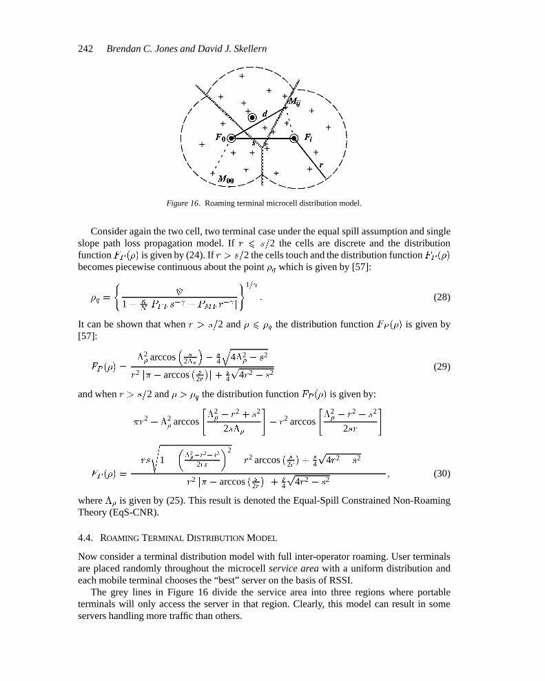
4.4. ROAMING TERMINAL DISTRIBUTION MODEL
Now consider a terminal distribution model with full inter-operator roaming. User terminalsare placed randomly throughout the microcell service area with a uniform distribution andeach mobile terminal chooses the “best” server on the basis of RSSI.
The grey lines in Figure 16 divide the service area into three regions where portableterminals will only access the server in that region. Clearly, this model can result in someservers handling more traffic than others.
wiremh03.tex; 9/12/1997; 12:02; v.5; p.20
An Integrated Propagation-Mobility Interference Model 243
Again consider the two cell, two terminal case under the equal spill assumption and singleslope path loss propagation model. The set of possible server admissions A is divided intotwo mutually exclusive events:
� S: The terminals choose the same server.� D: The terminals choose different servers.
The distribution functionFP (�) can thus be computed for this model using the total probabilitytheorem [58]:
FP (�) = FP (�jS)P (S) + FP (�jD)P (D): (31)
The distribution FP (�jD) is the Constrained Non-Roaming Terminal distribution given by(30). The distribution FP (�jS) is that resulting from same-cell interference. It can be shownthat when r > s=2 and � 6 �s the distribution FP (�jS) is given by [57]:
FP (�jS) =��2
�
r2�� � arccos
�s
2r
��+ s
4
p4r2 � s2
(32)
and when r > s=2 and �s < � 6 �r:
FP (�jS) =�2�
h� � arccos
�s
2��
�i+ s
4
q4�2
� � s2
r2�� � arccos
�s
2r
��+ s
4
p4r2 � s2
; (33)
where
�� =
�N
�PMF
� �� � 1
���1=
; (34)
�r =
(
1 + �N[PMF r� ]
)1=
; (35)
�s =
(
1 + �N [2 PMF s� ]
)1=
: (36)
Due to the symmetry of the two cell, two terminal system, clearly P (S) = P (D) = 0:5 thusFP (�) = 0:5[FP (�jS) + FP (�jD)]. The result is denoted the Equal-Spill Roaming Theory(EqS-R).
4.5. COMPARISON BETWEEN THE TERMINAL DISTRIBUTION MODELS – THEORETICAL
The three terminal distribution models may be compared by plotting their distribution functionsfor a specific case. Consider a two cell, two terminal CT2 system with the parameters as shownin Table 4. The CT2 system is assumed to be perfectly synchronised (i.e. all base stationstransmit at exactly the same time, so there is no fixed-to-fixed station interference).
A constant channel spill PMF of�49 dBc represents a situation where the DCA algorithmalways maintains 3 or more RF channels between the two CT2 links (the EqS theory). Inpractice, some terminals may use closer channels (even under DCA) that spill greater amountsof power and thus create more interference. Note also the single slope path loss model
wiremh03.tex; 9/12/1997; 12:02; v.5; p.21
244 Brendan C. Jones and David J. Skellern
Table 4. CT2 simulation parameters.
Parameter Value
3.0� �31.2 dBN �111.0 dBmPFF 0PMF �49 dBcr; s 100 m
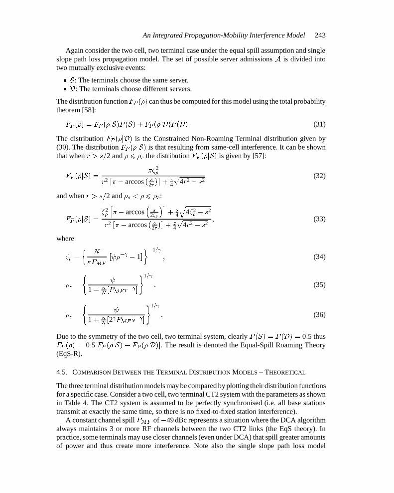
Figure 17. fH(�F ) for the three terminal distribution models.
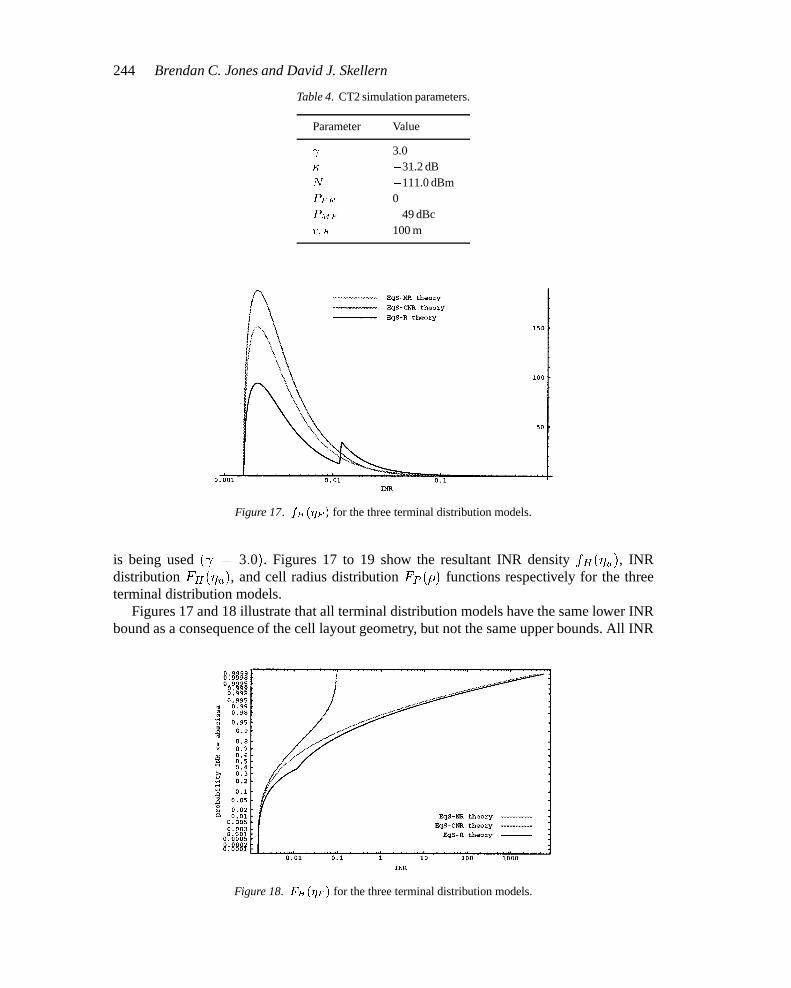
is being used ( = 3:0). Figures 17 to 19 show the resultant INR density fH(�u), INRdistribution FH(�u), and cell radius distribution FP (�) functions respectively for the threeterminal distribution models.
Figures 17 and 18 illustrate that all terminal distribution models have the same lower INRbound as a consequence of the cell layout geometry, but not the same upper bounds. All INR
Figure 18. FH(�F ) for the three terminal distribution models.
wiremh03.tex; 9/12/1997; 12:02; v.5; p.22
An Integrated Propagation-Mobility Interference Model 245
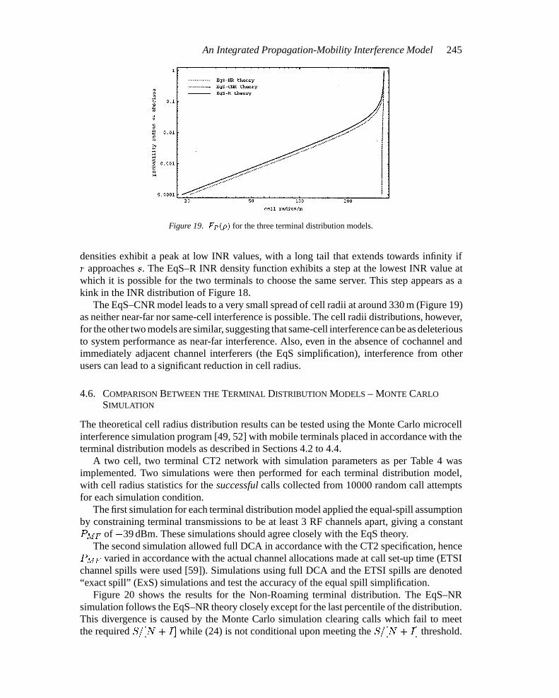
Figure 19. FP (�) for the three terminal distribution models.
densities exhibit a peak at low INR values, with a long tail that extends towards infinity ifr approaches s. The EqS–R INR density function exhibits a step at the lowest INR value atwhich it is possible for the two terminals to choose the same server. This step appears as akink in the INR distribution of Figure 18.
The EqS–CNR model leads to a very small spread of cell radii at around 330 m (Figure 19)as neither near-far nor same-cell interference is possible. The cell radii distributions, however,for the other two models are similar, suggesting that same-cell interference can be as deleteriousto system performance as near-far interference. Also, even in the absence of cochannel andimmediately adjacent channel interferers (the EqS simplification), interference from otherusers can lead to a significant reduction in cell radius.
4.6. COMPARISON BETWEEN THE TERMINAL DISTRIBUTION MODELS – MONTE CARLOSIMULATION
The theoretical cell radius distribution results can be tested using the Monte Carlo microcellinterference simulation program [49, 52] with mobile terminals placed in accordance with theterminal distribution models as described in Sections 4.2 to 4.4.
A two cell, two terminal CT2 network with simulation parameters as per Table 4 wasimplemented. Two simulations were then performed for each terminal distribution model,with cell radius statistics for the successful calls collected from 10000 random call attemptsfor each simulation condition.
The first simulation for each terminal distribution model applied the equal-spill assumptionby constraining terminal transmissions to be at least 3 RF channels apart, giving a constantPMF of �39 dBm. These simulations should agree closely with the EqS theory.
The second simulation allowed full DCA in accordance with the CT2 specification, hencePMF varied in accordance with the actual channel allocations made at call set-up time (ETSIchannel spills were used [59]). Simulations using full DCA and the ETSI spills are denoted“exact spill” (ExS) simulations and test the accuracy of the equal spill simplification.
Figure 20 shows the results for the Non-Roaming terminal distribution. The EqS–NRsimulation follows the EqS–NR theory closely except for the last percentile of the distribution.This divergence is caused by the Monte Carlo simulation clearing calls which fail to meetthe required S=[N + I] while (24) is not conditional upon meeting the S=[N + I] threshold.
wiremh03.tex; 9/12/1997; 12:02; v.5; p.23
246 Brendan C. Jones and David J. Skellern
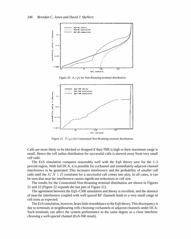
Figure 20. FP (�) for Non-Roaming terminal distribution.
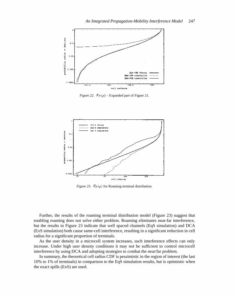
Figure 21. FP (�) for Constrained Non-Roaming terminal distribution.
Calls are more likely to be blocked or dropped if their INR is high or their maximum range issmall. Hence the cell radius distribution for successful calls is skewed away from very smallcell radii.
The ExS simulation compares reasonably well with the EqS theory save for the 1–5percent region. With full DCA, it is possible for cochannel and immediately-adjacent channelinterference to be generated. This increases interference and the probability of smaller cellradii until the S=[N + I] constraint for a successful call comes into play. In all cases, it canbe seen that near-far interference causes significant reductions in cell size.
The results for the Constrained Non-Roaming terminal distribution are shown in Figures21 and 22 (Figure 22 expands the last part of Figure 21).
The agreement between the EqS–CNR simulation and theory is excellent, and the absenceof near-far interference coupled with well spaced RF channels leads to a very small range ofcell sizes as expected.
The ExS simulation, however, bears little resemblance to the EqS theory. This discrepancy isdue to terminals in neighbouring cells choosing cochannels or adjacent channels under DCA.Such terminals can affect the system performance to the same degree as a close interfererchoosing a well-spaced channel (ExS-NR result).
wiremh03.tex; 9/12/1997; 12:02; v.5; p.24
An Integrated Propagation-Mobility Interference Model 247
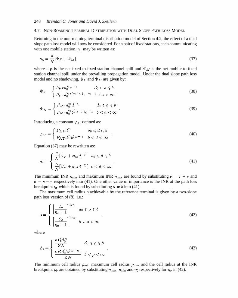
Figure 22. FP (�) – Expanded part of Figure 21.
Figure 23. FP (�) for Roaming terminal distribution.
Further, the results of the roaming terminal distribution model (Figure 23) suggest thatenabling roaming does not solve either problem. Roaming eliminates near-far interference,but the results in Figure 23 indicate that well spaced channels (EqS simulation) and DCA(ExS simulation) both cause same-cell interference, resulting in a significant reduction in cellradius for a significant proportion of terminals.
As the user density in a microcell system increases, such interference effects can onlyincrease. Under high user density conditions it may not be sufficient to control microcellinterference by using DCA and adopting strategies to combat the near/far problem.
In summary, the theoretical cell radius CDF is pessimistic in the region of interest (the last10% to 1% of terminals) in comparison to the EqS simulation results, but is optimistic whenthe exact spills (ExS) are used.
wiremh03.tex; 9/12/1997; 12:02; v.5; p.25
248 Brendan C. Jones and David J. Skellern
4.7. NON-ROAMING TERMINAL DISTRIBUTION WITH DUAL SLOPE PATH LOSS MODEL
Returning to the non-roaming terminal distribution model of Section 4.2, the effect of a dualslope path loss model will now be considered. For a pair of fixed stations, each communicatingwith one mobile station, �u may be written as:
�u =�
N[F +M ]; (37)
where F is the net fixed-to-fixed station channel spill and M is the net mobile-to-fixedstation channel spill under the prevailing propagation model. Under the dual slope path lossmodel and no shadowing, F and M are given by:
F =
(PFFd
10 s
� 1 d0 6 s 6 b
PFFd 10 b
( 2� 1)s� 2 b < s <1; (38)
M =
(PMFd
10 d
� 1 d0 6 d 6 b
PMFd 10 b
( 2� 1)d� 2 b < d <1: (39)
Introducing a constant 'M defined as:
'M =
(PMFd
10 d0 6 d 6 b
PMFd 10 b
( 2� 1) b < d <1: (40)
Equation (37) may be rewritten as:
�u =
8><>:
�
N[F + 'Md
� 1 ] d0 6 d 6 b
�
N[F + 'Md
� 2 ] b < d <1: (41)
The minimum INR �min and maximum INR �max are found by substituting d = r + s andd = s � r respectively into (41). One other value of importance is the INR at the path lossbreakpoint �b which is found by substituting d = b into (41).
The maximum cell radius � achievable by the reference terminal is given by a two-slopepath loss version of (8), i.e.:
� =
8>>><>>>:
� b
�u + 1
�1= 1
d0 6 � 6 b
� b
�u + 1
�1= 2
b < � <1; (42)
where
b =
8>><>>:�Ptd
10
ZNd0 6 � 6 b
�Ptd 10 b
( 2� 1)
ZNb < � <1
: (43)
The minimum cell radius �min maximum cell radius �max and the cell radius at the INRbreakpoint �b are obtained by substituting �max, �min and �b respectively for �u in (42).
wiremh03.tex; 9/12/1997; 12:02; v.5; p.26
An Integrated Propagation-Mobility Interference Model 249
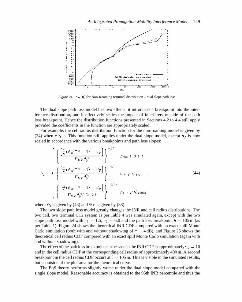
Figure 24. FH(�) for Non-Roaming terminal distribution – dual slope path loss.
The dual slope path loss model has two effects: it introduces a breakpoint into the inter-ference distribution, and it effectively scales the impact of interferers outside of the pathloss breakpoint. Hence the distribution functions presented in Sections 4.2 to 4.4 still applyprovided the coefficients in the function are appropriately scaled.
For example, the cell radius distribution function for the non-roaming model is given by(24) when r 6 s. This function still applies under the dual slope model, except �� is nowscaled in accordance with the various breakpoints and path loss slopes:
�� =
8>>>>>>>>>>>>>>><>>>>>>>>>>>>>>>:
8<:hN�( b�
� 1 � 1)�F
iPMFd
10
9=;�1= 1
�min 6 � 6 b
8<:hN� ( b�
� 2 � 1)�F
iPMFd
10
9=;�1= 1
b < � 6 �b
8<:hN� ( b�
� 2 � 1)�F
iPMFd
10 b
( 2� 1)
9=;�1= 2
�b < � 6 �max
; (44)
where b is given by (43) and F is given by (38).The two slope path loss model greatly changes the INR and cell radius distributions. The
two cell, two terminal CT2 system as per Table 4 was simulated again, except with the twoslope path loss model with 1 = 1:5, 2 = 6:0 and the path loss breakpoint b = 105 m (asper Table 1). Figure 24 shows the theoretical INR CDF compared with an exact spill MonteCarlo simulation (both with and without shadowing of � = 4 dB), and Figure 25 shows thetheoretical cell radius CDF compared with an exact spill Monte Carlo simulation (again withand without shadowing).
The effect of the path loss breakpoint can be seen in the INR CDF at approximately �u = 10and in the cell radius CDF at the corresponding cell radius of approximately 400 m. A secondbreakpoint in the cell radius CDF occurs at b = 105 m. This is visible in the simulated results,but is outside of the plot area for the theoretical curve.
The EqS theory performs slightly worse under the dual slope model compared with thesingle slope model. Reasonable accuracy is obtained to the 95th INR percentile and thus the
wiremh03.tex; 9/12/1997; 12:02; v.5; p.27
250 Brendan C. Jones and David J. Skellern
Figure 25. FP (�) for Non-Roaming terminal distribution – dual slope path loss.
Figure 26. Cochannel reuse ratio in FCA vs DCA systems.
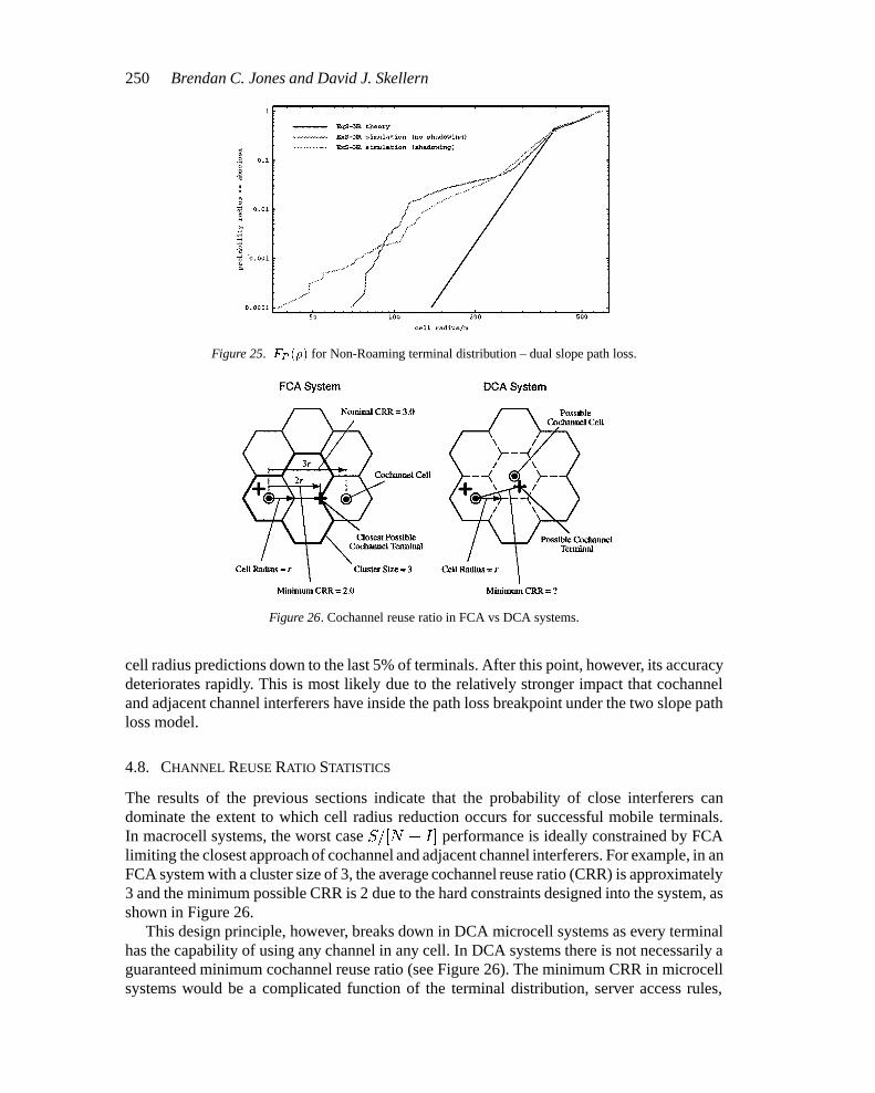
cell radius predictions down to the last 5% of terminals. After this point, however, its accuracydeteriorates rapidly. This is most likely due to the relatively stronger impact that cochanneland adjacent channel interferers have inside the path loss breakpoint under the two slope pathloss model.
4.8. CHANNEL REUSE RATIO STATISTICS
The results of the previous sections indicate that the probability of close interferers candominate the extent to which cell radius reduction occurs for successful mobile terminals.In macrocell systems, the worst case S=[N + I] performance is ideally constrained by FCAlimiting the closest approach of cochannel and adjacent channel interferers. For example, in anFCA system with a cluster size of 3, the average cochannel reuse ratio (CRR) is approximately3 and the minimum possible CRR is 2 due to the hard constraints designed into the system, asshown in Figure 26.
This design principle, however, breaks down in DCA microcell systems as every terminalhas the capability of using any channel in any cell. In DCA systems there is not necessarily aguaranteed minimum cochannel reuse ratio (see Figure 26). The minimum CRR in microcellsystems would be a complicated function of the terminal distribution, server access rules,
wiremh03.tex; 9/12/1997; 12:02; v.5; p.28
An Integrated Propagation-Mobility Interference Model 251
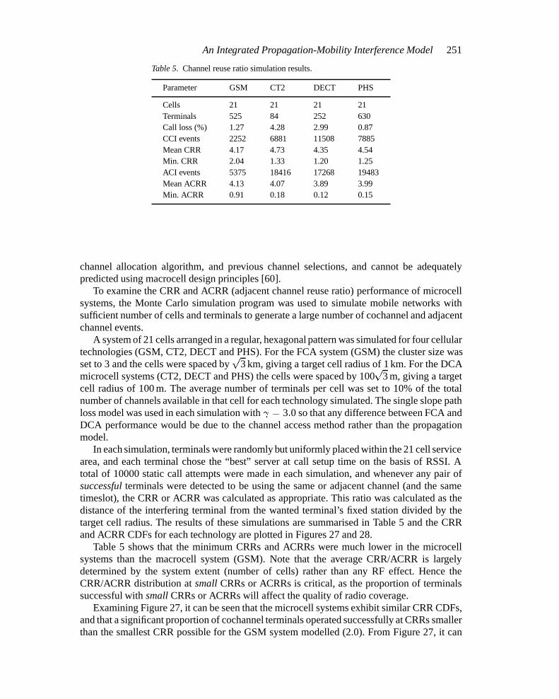
Table 5. Channel reuse ratio simulation results.
Parameter GSM CT2 DECT PHS
Cells 21 21 21 21Terminals 525 84 252 630Call loss (%) 1.27 4.28 2.99 0.87CCI events 2252 6881 11508 7885Mean CRR 4.17 4.73 4.35 4.54Min. CRR 2.04 1.33 1.20 1.25ACI events 5375 18416 17268 19483Mean ACRR 4.13 4.07 3.89 3.99Min. ACRR 0.91 0.18 0.12 0.15
channel allocation algorithm, and previous channel selections, and cannot be adequatelypredicted using macrocell design principles [60].
To examine the CRR and ACRR (adjacent channel reuse ratio) performance of microcellsystems, the Monte Carlo simulation program was used to simulate mobile networks withsufficient number of cells and terminals to generate a large number of cochannel and adjacentchannel events.
A system of 21 cells arranged in a regular, hexagonal pattern was simulated for four cellulartechnologies (GSM, CT2, DECT and PHS). For the FCA system (GSM) the cluster size wasset to 3 and the cells were spaced by
p3 km, giving a target cell radius of 1 km. For the DCA
microcell systems (CT2, DECT and PHS) the cells were spaced by 100p
3 m, giving a targetcell radius of 100 m. The average number of terminals per cell was set to 10% of the totalnumber of channels available in that cell for each technology simulated. The single slope pathloss model was used in each simulation with = 3:0 so that any difference between FCA andDCA performance would be due to the channel access method rather than the propagationmodel.
In each simulation, terminals were randomly but uniformly placed within the 21 cell servicearea, and each terminal chose the “best” server at call setup time on the basis of RSSI. Atotal of 10000 static call attempts were made in each simulation, and whenever any pair ofsuccessful terminals were detected to be using the same or adjacent channel (and the sametimeslot), the CRR or ACRR was calculated as appropriate. This ratio was calculated as thedistance of the interfering terminal from the wanted terminal’s fixed station divided by thetarget cell radius. The results of these simulations are summarised in Table 5 and the CRRand ACRR CDFs for each technology are plotted in Figures 27 and 28.
Table 5 shows that the minimum CRRs and ACRRs were much lower in the microcellsystems than the macrocell system (GSM). Note that the average CRR/ACRR is largelydetermined by the system extent (number of cells) rather than any RF effect. Hence theCRR/ACRR distribution at small CRRs or ACRRs is critical, as the proportion of terminalssuccessful with small CRRs or ACRRs will affect the quality of radio coverage.
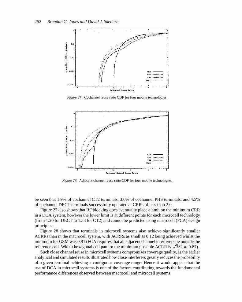
Examining Figure 27, it can be seen that the microcell systems exhibit similar CRR CDFs,and that a significant proportion of cochannel terminals operated successfully at CRRs smallerthan the smallest CRR possible for the GSM system modelled (2.0). From Figure 27, it can
wiremh03.tex; 9/12/1997; 12:02; v.5; p.29
252 Brendan C. Jones and David J. Skellern
Figure 27. Cochannel reuse ratio CDF for four mobile technologies.
Figure 28. Adjacent channel reuse ratio CDF for four mobile technologies.
be seen that 1.9% of cochannel CT2 terminals, 3.0% of cochannel PHS terminals, and 4.5%of cochannel DECT terminals successfully operated at CRRs of less than 2.0.
Figure 27 also shows that RF blocking does eventually place a limit on the minimum CRRin a DCA system, however the lower limit is at different points for each microcell technology(from 1.20 for DECT to 1.33 for CT2) and cannot be predicted using macrocell (FCA) designprinciples.
Figure 28 shows that terminals in microcell systems also achieve significantly smallerACRRs than in the macrocell system, with ACRRs as small as 0.12 being achieved whilst theminimum for GSM was 0.91 (FCA requires that all adjacent channel interferers lie outside thereference cell. With a hexagonal cell pattern the minimum possible ACRR is
p3=2 � 0:87).
Such close channel reuse in microcell systems compromises coverage quality, as the earlieranalytical and simulated results illustrated how close interferers greatly reduces the probabilityof a given terminal achieving a contiguous coverage range. Hence it would appear that theuse of DCA in microcell systems is one of the factors contributing towards the fundamentalperformance differences observed between macrocell and microcell systems.
wiremh03.tex; 9/12/1997; 12:02; v.5; p.30
An Integrated Propagation-Mobility Interference Model 253
5. Conclusion
This paper has presented a new interference model for microcellular networks which can beused to model microcell coverage performance in terms of the broad system design parametersincluding propagation model, terminal distribution, cell spacing, user load, and channel spill.
Monte Carlo simulations and mathematical analysis have shown that DCA microcellsystems are more highly interference limited, exhibit a greater cell radius variation, andhave closer frequency reuse than FCA macrocell systems. These characteristics suggest thatachieving reliable contiguous coverage in microcell systems will be difficult and will requirea design approach different to that used in macrocell FCA systems.
In order to design a microcell system to meet given service quality targets, it has beenproposed that the interference and cell radius statistics need to be derived or numericallyestimated. It is proposed that the interference statistics obtained from the model provide abasis for determining the call blocking performance of the system, and that the cell radiusstatistics provide a basis for determining the cell spacing required in order to meet a coveragetarget for the offered user load. Developing these techniques could form the basis of a microcelldesign methodology.
Appendix – Notation and Acronym Glossary
Latin Notation
ACI Adjacent Channel InterferenceACRR Adjacent Channel Reuse RatioAMPS Advanced Mobile Phone Service (US analog macrocell standard)b Breakpoint in the dual slope path loss modelC Cluster size in an FCA systemCij Duplex channel comprising an uplink channel CUij and a downlink channel CDij
CDij Downlink channel ij (transmission from fixed station Fi to mobile terminal Mij )CUij Uplink channel ij (transmission from mobile terminal Mij to fixed station Fi)CDF Cumulative Distribution FunctionCRR Cochannel Reuse RatioCT2 Cordless Telephone 2nd generation (digital microcell)d Distance variabled0 Reference distance in the distance-dependent path loss propagation modelDCA Dynamic Channel AssignmentDECT Digital European Cordless Telephone (digital microcell);Fi Fixed Station iFCA Fixed Channel AssignmentFDMA Frequency Division Multiple AccessGr; Gt Receiver and Transmitter antenna gainGSM Groupe Special Mobile (also called Global System for Mobiles) (digital macrocell)hr; ht Receiver and Transmitter antenna heightsIFij Total interference power received in channel CUij at fixed station FiIFFij Interference power received from all fixed stations in channel CUij at FiIFMij Interference power received from all fixed stations in channel CDij at Mij
IMij Total interference power received in channel CDij at mobile terminal Mij
IMFij Interference power received from all mobile terminals in channel CUij at FiIMMij Interference power received from all mobile terminals in channel CDij at Mij
INR Interference to Noise Ratio (given the symbol � in equations)K;Kd; Ku Relative interferer strength. Kd = Pt=ZPd (downlink), Ku = Pt=ZPu (uplink)Mij Mobile terminal j communicating with fixed station FiN RMS Receiver Noise PowerPd Spill power into a wanted downlink (general)PFij Transmit power from fixed station Fi to mobile terminal Mij
PFF Fixed station to fixed station spill power (general)
wiremh03.tex; 9/12/1997; 12:02; v.5; p.31
254 Brendan C. Jones and David J. Skellern
PFM Fixed station to mobile terminal spill power (general)PMij Transmit power from mobile terminal Mij to fixed station FiPr Received power (general)Ps Channel Spill power (general)Pt Transmitted power (general)Pu Spill power into a wanted uplink (general)PXijY kl Channel spill from Xij to Ykl (Xij is the transmitter and Ykl the receiver)PDF Probability Density FunctionPHS Personal Handy phone System (Japan) (digital microcell)r Cell radius (intended or target cell radius, usually a function of cell spacing)rd; ru Mobile terminal range at downlink and uplink failure (respectively)ri;k Distance between fixed station Fi and fixed station Fkrij;k Distance between mobile terminal Mij and fixed station Fkrij;kl Distance between mobile terminal Mij and mobile terminal Mkl
RSSI Received Signal Strength Indications Fixed station separation (general)S=I Signal to Interference RatioS=[N + I] Signal to Noise plus Interference RatioTDD Time Division DuplexTDMA Time Division Multiple AccessZ System interference protection ratio
Greek Notation
� Outage range relative to fixed station separation Path loss exponent in a distance-dependent path loss propagation model 1; 2 First and second path loss exponents in the dual slope path loss propagation model� Interference to Noise Ratio (general)�c The uplink INR value at which the uplink and downlink outage contours intersect at a single point�e The uplink INR value at which the interferer is first enclosed by the downlink outage contour�u Uplink Interference to Noise Ratio (i.e. at a fixed station)�d Downlink Interference to Noise Ratio (i.e. at a mobile terminal)� The free space path loss from a transmit antenna to the reference distance d0
� Wavelength of radio transmission� Maximum cell radius achievable by a mobile terminal� Standard deviation of signal power in dB in the lognormal shadowing model� Normally distributed dB variable in the lognormal shadowing model'M Path loss constant in the dual slope path loss model Technology dependent system constant = �Pt=ZN b Technology dependent system constant in the dual slope path loss modelF ;M Net fixed to fixed station channel spill and mobile to fixed channel spill (respectively)
References
1. W.R. Young, “Advanced Mobile Phone Service: Introduction, Background and Objectives”, Bell SystemTechnical Journal, Vol. 58 No. 1 pp. 1–14, Jan. 1979.
2. G. Calhoun, Digital Cellular Radio, Artech House, Massachusetts, USA, 1988.3. J.D. Parsons and J.G. Gardiner, Mobile Communications Systems, Blackie and Sons, London, 1989.4. J. Sarnecki, C. Vinodrai, A. Javed, P. O’Kelly and K. Dick, “Microcell Design Principles”, IEEE Communi-
cations Magazine, Vol. 31 No. 4 pp. 76–82, April 1993.5. D.C. Cox, “Wireless Network Access for Personal Communications”, IEEE Communications Magazine,
pp. 96-115, Dec. 1992.6. T.S. Rappaport, “Wireless Personal Communications: Trends and Challenges”, IEEE Antennas and Propa-
gation Magazine, Vol. 33 No. 5 pp. 19–29, Oct. 1991.7. A. Gamst, “Remarks on Radio Network Planning”, Proceedings of the 37th IEEE Vehicular Technology
Conference, p. 164, Tampa, 1–3 June 1987.
wiremh03.tex; 9/12/1997; 12:02; v.5; p.32

An Integrated Propagation-Mobility Interference Model 255
8. W.C.Y. Lee, “Smaller Cells for Greater Performance”, IEEE Communications Magazine, Vol. 29 No. 11pp. 19–23, Nov. 1991.
9. W.C.Y. Lee, “Quality and Capacity in Cellular”, Electro International Conference Record, pp. 519–20, NewYork, USA, 16–18 Apr. 1991.
10. W.C.Y. Lee, “Spectrum Efficiency in Cellular”, IEEE Transactions on Vehicular Technology, Vol. 38 No. 2pp. 69–75, May 1989.
11. W.C.Y. Lee, “Estimate of Channel Capacity in Rayleigh Fading Environment”, IEEE Transactions on Vehic-ular Technology, Vol. 39 No. 3 pp. 187–189, Aug. 1990.
12. J.G. Gardiner, “Second Generation Cordless (CT2) Telephony in the UK: Telepoint Services and the commonair interface”, Electronics and Communication Engineering Journal, pp. 71–78, April 1990.
13. I. Goetz, “Transmission Planning for Mobile Telecommunication Systems”, 6th IEE International Conferenceon Mobile Radio and Personal Communications, pp. 126–130, Coventry, UK, 9–11 Dec. 1991.
14. V.H. MacDonald, “The Cellular Concept”, Bell System Technical Journal, Vol. 58 No. 1 pp. 15–41, Jan.1979.
15. W.C.Y. Lee, Mobile Communications Design Fundamentals, 2nd Ed., John Wiley and Sons, New York, 1993.16. W.T. Webb, “Modulation Methods for PCNs”, IEEE Communications Magazine, Vol. 30 No. 12 pp. 90-95,
Dec 1992.17. S.-W. Wang and S.S. Rappaport, “Signal to Interference Calculations for Corner Excited Cellular Commu-
nications Systems”, IEEE Transactions on Communications, Vol. 39 No. 12 pp. 1886–1896, Dec. 1991.18. S.-W. Wang and S.S Rappaport, “Signal to Interference Calculations for Balanced Channel Assignment
Patterns in Cellular Communications Systems”, IEEE Transactions on Communications, Vol. 37 No. 10pp. 1077–1087, Oct. 1989.
19. J.P. Driscoll, “Relevance of Receiver Filter Perfrmance and Operating Range for CT2/CAI Telepoint Sys-tems”, Electronics Letters, Vol. 28 No. 13 pp. 1200–1201, 18 June 1992.
20. J.P. Driscoll, “Some Factors Which Affect the Traffic Capacity of a Small Telepoint Network”, 5th IEEInternational Conference on Mobile Radio and Personal Communications, pp. 167–71, Coventry, UK, 11–14Dec. 1989.
21. D. Everitt and D. Manfield, “Performance Analysis of Cellular Mobile Communications Systems withDynamic Channel Assignment”, IEEE Journal on Selected Areas of Communications, Vol. 7 No. 8 pp. 1172–1180, Oct. 1989.
22. A.O. Fapojuwo, A. McGirr and S. Kazeminejad, “A Simulation Study of Speech Traffic Capacity in DigitalCordless Telecommunications Systems”, IEEE Transactions on Vehicular Technology, Vol. 41 No. 1 pp. 6–16,Feb. 1992.
23. P.A. Ramsdale, A.D. Hadden and P.S. Gaskell, “DCS1800 – The Standard for PCN”, 6th IEE InternationalConference on Mobile Radio and Personal Communications, pp. 175–179, Coventry, UK, 9–11 Dec. 1991.
24. P.T.H. Chan, M. Palaniswami and D. Everitt, “Dynamic Channel Assignment for Cellular Mobile RadioSystem using Self-Organising Neural Networks”, 6th Australian Teletraffic Research Seminar, pp. 89–95,Wollongong, Australia, 28–29 Nov. 1991.
25. S. Sato, K. Takeo, M. Nishino, Y. Amezawa and T. Suzuki, “A Performance Analysis on Nonuniform Trafficin Microcell Systems”, IEEE International Conference on Communications (ICC 93), Vol. 3 pp. 1960–1964,Geneva, Switzerland, 23–26 May 1993.
26. S.T.S. Chia, “The Universal Mobile Telecommunication System”, IEEE Communications Magazine, Vol. 30No. 12 pp. 54–62, Dec. 1992.
27. S.T.S. Chia, “Providing Ubiquitous Cellular Coverage for a Dense Urban Environment”, 44th VehicularTechnology Conference, pp. 1045–1049, Stockholm, Sweden, 8–10 June 1994.
28. A. Kegel, W. Hollemans and R. Prasad, “Performance Analysis of Interference and Noise Limited CellularLand Mobile Radio”, 41st IEEE Vehicular Technology Conference, pp. 817–821, St Louis, USA, 19–22 May1991.
29. J.-P.M.G. Linnartz, “Exact Outage Analysis of the Outage Probability in Multiple-User Mobile Radio”, IEEETransactions on Communications, Vol. 40 No. 1, pp. 20–23, January 1992.
30. J.C.-I. Chuang, “Performance Limitations of TDD Wireless Personal Communications with AsynchronousRadio Ports”, Electronics Letters, Vol. 28 No. 6, pp. 532–534, 12 March 1992.
31. Y.-D. Yao and A.U.H. Sheikh, “Outage Probability Analysis for Microcell Radio Systems with CochannelInterferers in Rician/Rayleigh Fading Environment”, Electronics Letters, Vol. 26 No. 13, pp. 864–866, 21June 1990.
32. Y.-D. Yao and A.U.H. Sheikh, “Bit Error Probabilities of NCFSK and DPSK Signals in Microcellular MobileRadio Systems”, Electronics Letters, Vol. 28 No. 4, pp. 363–364, 13 February 1992.
33. Y.-D. Yao and A.U.H. Sheikh, “Performance Analyses of Microcellular Mobile Radio Systems with ShadowedCochannel Interferers”, Electronics Letters, Vol. 28 No. 9, pp. 839–841, 23 April 1992.
wiremh03.tex; 9/12/1997; 12:02; v.5; p.33
256 Brendan C. Jones and David J. Skellern
34. Y.-D. Yao and A.U.H. Sheikh, “Investigation into Cochannel Interference in Microcellular Mobile RadioSystems”, IEEE Transactions on Vehicular Technology, Vol. 41 No. 2, pp. 114–123, May 1992.
35. R. Prasad, A. Kegel, J. Olsthoorn, “Spectrum Efficiency Analysis for Microcellular Mobile Radio Systems”,Electronics Letters, Vol. 27 No. 5, pp. 423–425, 28 February 1991.
36. R. Prasad, A. Kegel and M.B. Loog, “Cochannel Interference Probability for Picocellular System withMultiple Rician Faded Interferers”, Electronics Letters, Vol. 28 No. 24, pp. 2225–2226, 19 November1992.
37. K.W. Sowerby and A.G. Williamson, “Outage Probabilities in Mobile Radio Systems Suffering CochannelInterference”, IEEE Journal on Selected Areas in Communications, pp. 516–522, Vol. 10 No. 3, April1992.
38. J.E. Button, “Performance of CT2/CAI Systems in Small Cell Environments”, Electronics Letters, Vol. 26No. 18, pp. 1434–1436, 30 August 1990.
39. J.E. Button, “Asynchronous CT2/CAI Telepoint Separation Requirements”, Electronics Letters, Vol. 27 No. 1,pp. 48–49, 3 January 1991.
40. C.E. Cook, “Modelling Interference Effects for Land Mobile and Air Mobile Communications”, IEEETransactions on Communications, Vol. 35 No. 2 pp. 151–165, Feb. 1987.
41. G.C. Hess, Land-Mobile Radio System Engineering, Artech House, Boston, 1993.42. M.J. Feuerstein, K.L. Blackard, T.S. Rappaport, S.Y. Seidel and H.H. Xia, “Path Loss, Delay Spread and
Outage Models as Functions of Antenna Height for Microcellular System Design”, IEEE Transactions onVehicular Technology, Vol. 43 No. 3 pp. 487–498, Aug. 1994.
43. H.H. Xia, H.L. Bertoni, L.R. Maciel, A. Lindsay-Stewart and R. Rowe, “Microcellular Propagation Character-istics for Personal Communications in Urban and Suburban Environments”, IEEE Transactions on VehicularTechnology, Vol. 43 No. 3, pp. 743–751, Aug. 1994.
44. H.H. Xia, H.L. Bertoni, L.R. Maciel, A. Lindsay-Stewart and R. Rowe, “Radio Propagation Characteristicsfor Line-of-Sight and Personal Communications”, IEEE Transactions on Antennas and Propagation, Vol. 41No. 10 pp. 1439–1447, Oct. 1993.
45. V. Erceg, S. Ghassemzadeh, M. Taylor, D. Li and D.L. Schilling, “Urban/Suburban Out-of-sight PropagationModelling”, IEEE Communications Magazine, Vol. 30 No. 6 pp. 56–61, June 1992.
46. E. Green, “Radio Link Design for Microcellular Systems”, British Telecom Technology Journal, Vol. 8 No. 1pp. 85–96, Jan. 1990.
47. W.C. Jakes, Microwave Mobile Communications, IEEE Press, New York, 1974.48. B.C. Jones and D.J. Skellern, “Interference Modelling and Outage Contours in Cellular and Microcellular
Networks”, 2nd MCRC International Conference on Mobile and Personal Communications Systems, pp. 149–158, Adelaide, Australia, 10–11 April 1995.
49. B.C. Jones and D.J. Skellern, “Spatial Outage Analysis in Cellular and Microcellular Networks”, pp. 1–18,Wireless ’95, Calgary, Canada, 10–12 July 1995.
50. E.H. Lockwood, A Book Of Curves, Cambridge University Press, England, 1967.51. B.C. Jones and D.J. Skellern, “Designing the Ubiquitous Microcellular Network”, Workshop on Applications
of Radio Science (WARS ’95), pp. I.8.1–I.8.4, Canberra, Australia, 25–27 June 1995.52. B.C. Jones and D.J. Skellern, “Outage Contours and Cell Size Distributions in Cellular and Microcellular
Networks”, pp. 145–149, 45th IEEE Vehicular Technology Conference (VTC ’95), Chicago, United States,26–28 July 1995.
53. M.J. Marsan, G.C. Hess and S.S. Gilbert, “Shadowing variability in an Urban Land Mobile Environment at900 MHz”, Electronics Letters, Vol. 26 No. 10, pp. 646–648, 10 May 1990.
54. S.Y. Seidel, T.S. Rappaport, “Path Loss and Multipath Delay Statistics in Four European Cities for 900 MHzCellular and Microcellular Communications”, Electronics Letters, Vol. 26 No. 20 pp. 1713–1715, 27 Sept.1990.
55. B.C. Jones and D.J. Skellern, “System Design for Contiguous Coverage in High Density MicrocellularNetworks”, International Symposium on Signals, Systems and Electronics (ISSSE ’95), pp. 263–266, SanFrancisco, United States, 25–27 October 1995.
56. B.C. Jones and D.J. Skellern, “Interference Distributions in Microcell Ensembles”, 6th IEEE InternationalSymposium on Personal, Indoor and Mobile Radio Communications (PIMRC ’95), pp. 1372–1376, Toronto,Canada, 27–29 September 1995.
57. B.C. Jones and D.J. Skellern, “Influence of Terminal Distributions and Channel Spills on Microcell Coverage”,IEEE 1995 Global Telecommunications Conference (Globecom ’95), pp. 17–21, Singapore, 13–17 November1995.
58. A. Papoulis, Probability, Random Variables and Stochastic Processes, 3rd Ed., McGraw Hill, New York,1991.
wiremh03.tex; 9/12/1997; 12:02; v.5; p.34
An Integrated Propagation-Mobility Interference Model 257
59. European Telecommunications Standards Institute (ETSI), “Common Air Interface Specification betweencordless telephone apparatus in the frequency band 864.1 MHz to 868.1 MHz”, I-ETS 300–131, September1991.
60. R. Saunders and L. Lopes, “Performance Comparison of Global and Distributed Dynamic Channel AllocationAlgorithms”, pp. 799-803, 44th IEEE Vehicular Technology Conference (VTC ’94), Stockholm, Sweden,8–10 June 1994.
Brendan Jones graduated in Electrical Engineering with First Class Honours from NewcastleUniversity, Australia, in 1986, and was awarded second prize in the IEEE Region 10 Under-graduate Student Paper Competition that year. From 1987 to 1993 he worked in the Researchand Development division of OTC Australia, one of Australia’s international telecommunica-tions carriers, and was involved in many research projects including microcellular modellingwork for the OTC/Chevalier CT2 network in Hong Kong. From 1993 to 1996 he completed aPhD at Macquarie University in Sydney, Australia, investigating the modelling and analysisof interference in microcellular networks. In 1996 he was awarded first prize in both theRegion 10 and Australia/New Zealand IEEE Postgraduate Student Paper Competitions. Henow works for Optus Communications, Australia’s second largest telecommunications com-pany, as a technical specialist in mobile network planning. He has had over fifteen paperspublished.
David Skellern is the Professor of Electronics at Macquarie University. He holds the BSc(1972), BE (1974) and PhD (1985) degrees from the University of Sydney, Australia. From1974 to 1983 he held various positions at the University of Sydney’s Fleurs Radio Observatory.
wiremh03.tex; 9/12/1997; 12:02; v.5; p.35
258 Brendan C. Jones and David J. Skellern
His research since the mid 1980s, both in Australia and overseas, has involved collaborationwith industry and research organisations on communications systems, circuit, and devicedesign. At Macquarie University he has overseen major research programs in microelectronics,wireless communications networks and integrated services and is the author or co-author ofover 30 journal articles and 80 conference papers in these research areas. Professor Skellernin the Chairman of the National Committee for Radio Science of the Australian Academy ofScience, the Australian representative on Commission D (Electronic and Optical Devices andApplications) of the International Union for Radio Science (URSI), and a former Chairmanof the Australian Telecommunications and Electronics Research Board.
wiremh03.tex; 9/12/1997; 12:02; v.5; p.36