An Integrative Bayesian Modeling Approachto Imaging Genetics

Francesco C. STINGO, Michele GUINDANI, Marina VANNUCCI, and Vince D. CALHOUN

In this article we present a Bayesian hierarchical modeling approach for imaging genetics, where the interest lies in linking brain connectivityacross multiple individuals to their genetic information. We have available data from a functional magnetic resonance imaging (fMRI) studyon schizophrenia. Our goals are to identify brain regions of interest (ROIs) with discriminating activation patterns between schizophrenicpatients and healthy controls, and to relate the ROIs’ activations with available genetic information from single nucleotide polymorphisms(SNPs) on the subjects. For this task, we develop a hierarchical mixture model that includes several innovative characteristics: it incorporatesthe selection of ROIs that discriminate the subjects into separate groups; it allows the mixture components to depend on selected covariates;it includes prior models that capture structural dependencies among the ROIs. Applied to the schizophrenia dataset, the model leads to thesimultaneous selection of a set of discriminatory ROIs and the relevant SNPs, together with the reconstruction of the correlation structure ofthe selected regions. To the best of our knowledge, our work represents the first attempt at a rigorous modeling strategy for imaging geneticsdata that incorporates all such features.

KEY WORDS: Bayesian hierarchical model; Functional magnetic resonance imaging; Markov random field; Neuroimaging; Single-nucleotide polymorphism; Variable selection.

1. INTRODUCTION

Functional magnetic resonance imaging (fMRI) is a com-mon tool for detecting changes in neuronal activity. It measuresblood oxygenation level-dependent (BOLD) contrast that de-pends on changes in the regional cerebral blood-flow (rCBF).fMRI has become very popular in the neuroimaging field dueto its relatively low invasiveness, absence of radiation exposure,and relatively wide applicability.

Statistical methods play an important role in the analysis offMRI data and have generated a growing literature (see e.g.,Lazar 2008; Lindquist 2008, for reviews on methods). Dimen-sion reduction techniques, such as principal component analysis(PCA) and independent component analysis (ICA), and cluster-ing algorithms are routinely applied to imaging data as a wayof mapping connectivity. In the fMRI literature, connectivityrefers to parts of the brain that show similarities and/or that inter-act with each other. In particular, anatomical connectivity dealswith how different brain regions are physically connected; func-tional connectivity is defined as the association, or correlation,between fMRI time series of distinct voxels or regions; while ef-fective connectivity is the directed influence of one brain regionon others (Friston 1994). Because of the high-dimensionalityof the data, that is, the large number of voxels, studies oftenperform region-based analyses, by looking at specific regionsof interest (ROIs), or by dividing the entire brain into ROIs, forexample, by parcellating the brain into anatomical regions (see,e.g., Tzourio-Mazoyer et al. 2002). Bayesian approaches haverecently found successful applications in the fMRI field (Smith

Francesco C. Stingo, The University of Texas MD Anderson CancerCenter, Houston, TX 77230 (E-mail: FStingo@mdanderson.org). MicheleGuindani, The University of Texas MD Anderson Cancer Center, Hous-ton, TX 77230 (E-mail: mguindani@mdanderson.org). Marina Vannucci isProfessor, Department of Statistics, Rice University, Houston, TX 77005(E-mail: marina@rice.edu). Vince D. Calhoun, Departments of Electri-cal and Computer Engineering (primary), Neurosciences, Computer Sci-ence, and Psychiatry, University of New Mexico, Albuquerque, NM 87131(E-mail: vcalhoun@unm.edu). Marina Vannucci’s research was partially fundedby NIH/NHLBI P01-HL082798 and NSF/DMS 1007871. Vince Calhoun’s re-search was partially funded by NIH R01EB005846 and 5P20RR021938.

et al. 2003; Woolrich et al. 2004, 2009; Penny, Trujillo-Barreto,and Friston 2005; Bowman et al. 2008; Guo, Bowman, and Kilts2008). Also, nonparametric Bayesian methods that cluster brainregions on the basis of their connectivity patterns have beenproposed (Jbabdi, Woolrich, and Behrens 2009). Compared toother inferential approaches and algorithmic procedures com-monly used in the analysis of fMRI data, Bayesian methodsallow for a direct assessment of the uncertainties in the parame-ters’ estimates and, perhaps more importantly, the incorporationof prior knowledge, such as on spatial correlation among voxelsand/or ROIs, into the model.

In this article we consider a problem of imaging genetics,where structural and functional neuroimaging is applied tostudy subjects carrying genetic risk variants that relate to apsychiatric disorder. Our work, in particular, is motivated by adataset on subjects diagnosed with schizophrenia and healthycontrols, collected as part of the Mind Clinical Imaging Con-sortium (MCIC; Chen et al. 2012), where we have availablemeasurements on fMRI scans and single nucleotide polymor-phism (SNP) allele frequencies on all participants. The fMRIdata were collected during a sensorimotor task, a block-designmotor response to auditory stimulation. The resulting imageswere realigned, normalized, and spatially smoothed as custom-ary, to remove most nontask-related sources of variability fromthe data (Ashby 2011; Chen et al. 2012). Here, the fMRI in-formation is further summarized in individual contrast imagesof ROI-based summary statistics, as follows. For each partici-pant, we fit a multiple regression incorporating regressors of thestimulus and its temporal derivative plus an intercept term. Theresulting coefficient estimates can be used to build individualsynthetic brain maps capturing the stimulus effect at each voxel.The maps are then superimposed to a fixed template atlas, forexample, the MNI space automated anatomical labeling (AAL)atlas (Tzourio-Mazoyer et al. 2002), and additionally segmented

© 2013 American Statistical AssociationJournal of the American Statistical Association

September 2013, Vol. 108, No. 503, Applications and Case StudiesDOI: 10.1080/01621459.2013.804409

876

Stingo et al.: Bayesian Modeling Approach to Imaging Genetics 877

into automatically labeled ROIs. Summary statistics, as the me-dian or maximum intensity values, can be computed over thevoxels included in each region (Kim et al. 2005; Etzel, Gazzola,and Keysers 2009). In addition to the fMRI data, we also haveavailable measurements on SNP allele frequencies on all sub-jects. We use the genetic data as potential covariates that mayaffect brain function, in both healthy controls and patients withschizophrenia.

The goal of our analysis is to detect local activations, thatis, areas of increased BOLD signal in response to a stimu-lus, by selecting a subset of ROIs that explain the observedactivation patterns, and to identify SNPs that might be rele-vant to explain such activations. Understanding how connec-tivity varies between schizophrenic and control subjects is ofutmost importance for diagnostic purposes and therapeutic in-terventions. The ability to link the imaging and genetic com-ponents in the participants’ subgroups could lead to improveddiagnostic tools and therapies, as it is now generally recog-nized that brain connectivity is affected by genetic character-istics (Colantuoni et al. 2008; Liu et al. 2009). Indeed, Chenet al. (2012) found evidence of a significant correlation be-tween fMRI and SNP data. These authors use a two-step pro-cedure involving a combination of PCA and ICA techniques,whereas we propose to study the association between spatialpatterns and genetic variations across individuals within the co-herent probabilistic framework offered by Bayesian hierarchicalmodels.

We develop a hierarchical mixture model that includes severalinnovative characteristics. First, it incorporates the selection ofROIs that discriminate the subjects between schizophrenic pa-tients and healthy controls, allowing for a direct assessment ofthe uncertainties in the estimates of the model selection parame-ters. Second, it allows the group-specific distributions to dependon selected covariates, that is, the SNP data. In this sense, ourproposed model is integrative, in that it combines the observedbrain activation patterns with the subjects’ specific genetic in-formation. Third, it incorporates prior knowledge via networkmodels that capture known dependencies among the ROIs. Morespecifically, it employs spatially defined selection process pri-ors that capture available knowledge on connectivity amongregions of the brain, so that regions having the same activationpatterns are more likely to be selected together. Furthermore,our hierarchical formulation accounts for additional correlationamong selected ROIs that may not be captured by the networkprior. Applied to the schizophrenia dataset, the model allowsthe simultaneous selection of a set of discriminatory ROIs andthe relevant SNPs, together with the reconstruction of the de-pendence structure of the selected regions. To the best of ourknowledge, our work represents the first attempt at a rigorousmodeling strategy for imaging genetics data that incorporatesall such characteristics.

The remainder of the article is organized as follows: In Sec-tion 2, we introduce our modeling framework and its majorcomponents. We describe posterior inference and prediction inSection 3. In Section 4, we first assess performances of ourproposed model on simulated data and then investigate resultson data from our case study on schizophrenia. We conclude thearticle with some remarks in Section 5.

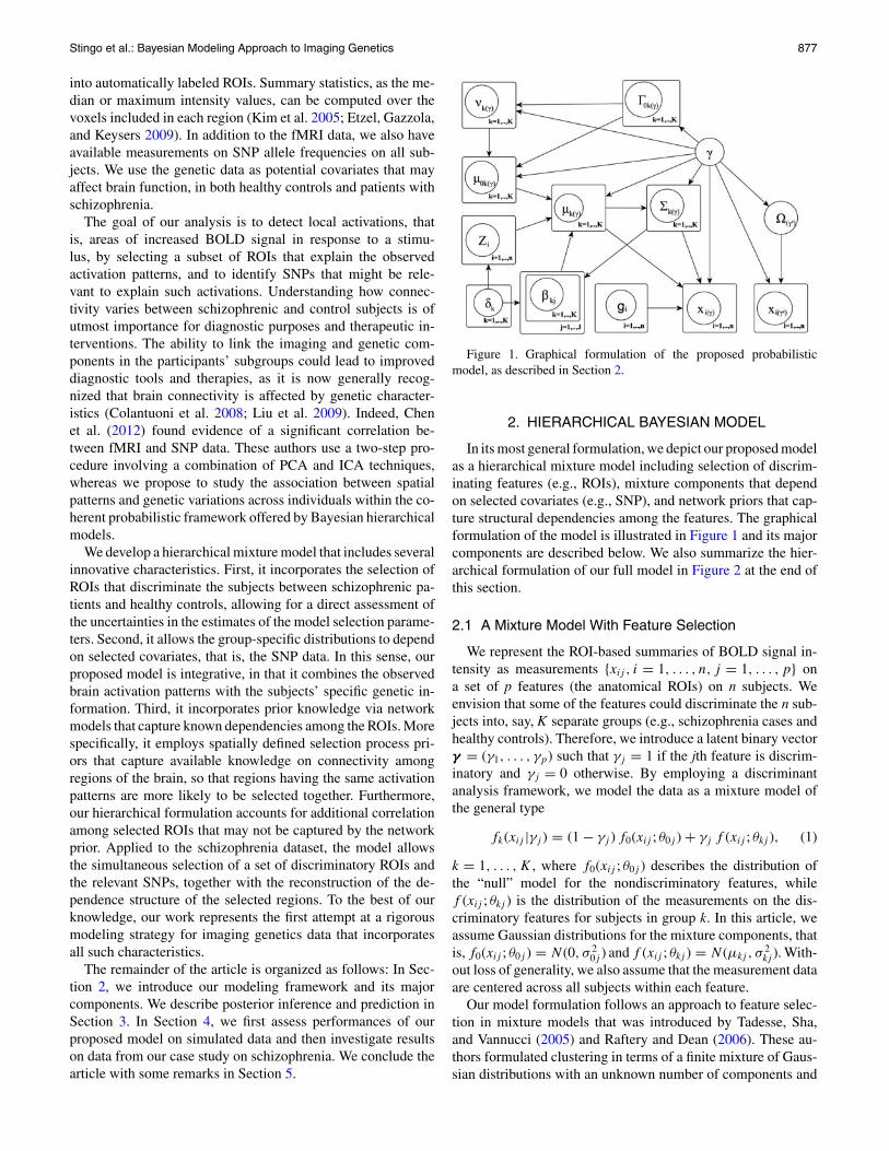
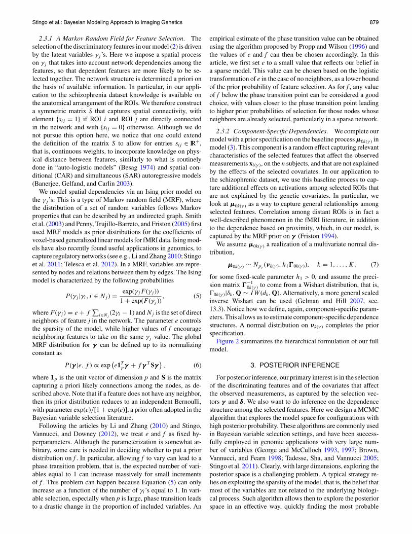
Figure 1. Graphical formulation of the proposed probabilisticmodel, as described in Section 2.

2. HIERARCHICAL BAYESIAN MODEL

In its most general formulation, we depict our proposed modelas a hierarchical mixture model including selection of discrim-inating features (e.g., ROIs), mixture components that dependon selected covariates (e.g., SNP), and network priors that cap-ture structural dependencies among the features. The graphicalformulation of the model is illustrated in Figure 1 and its majorcomponents are described below. We also summarize the hier-archical formulation of our full model in Figure 2 at the end ofthis section.

2.1 A Mixture Model With Feature Selection

We represent the ROI-based summaries of BOLD signal in-tensity as measurements {xij , i = 1, . . . , n, j = 1, . . . , p} ona set of p features (the anatomical ROIs) on n subjects. Weenvision that some of the features could discriminate the n sub-jects into, say, K separate groups (e.g., schizophrenia cases andhealthy controls). Therefore, we introduce a latent binary vectorγγγ = (γ1, . . . , γp) such that γj = 1 if the jth feature is discrim-inatory and γj = 0 otherwise. By employing a discriminantanalysis framework, we model the data as a mixture model ofthe general type

fk(xij |γj ) = (1 − γj ) f0(xij ; θ0j ) + γj f (xij ; θkj ), (1)

k = 1, . . . , K , where f0(xij ; θ0j ) describes the distribution ofthe “null” model for the nondiscriminatory features, whilef (xij ; θkj ) is the distribution of the measurements on the dis-criminatory features for subjects in group k. In this article, weassume Gaussian distributions for the mixture components, thatis, f0(xij ; θ0j ) = N (0, σ 2

0j ) and f (xij ; θkj ) = N (µkj , σ2kj ). With-

out loss of generality, we also assume that the measurement dataare centered across all subjects within each feature.

Our model formulation follows an approach to feature selec-tion in mixture models that was introduced by Tadesse, Sha,and Vannucci (2005) and Raftery and Dean (2006). These au-thors formulated clustering in terms of a finite mixture of Gaus-sian distributions with an unknown number of components and

878 Journal of the American Statistical Association, September 2013

then introduced latent variables to identify discriminating fea-tures. Kim, Tadesse, and Vannucci (2006) proposed an alterna-tive modeling approach that uses infinite mixture models viaDirichlet process priors. Also, Hoff (2006) adopted a mixture ofGaussian distributions where different clusters were identifiedby mean shifts and where discriminating features were identi-fied via the calculation of Bayes factors. Stingo, Vannucci, andDowney (2012) extended the approach by Tadesse, Sha, andVannucci (2005) and Raftery and Dean (2006) to the discrim-inant analysis framework. Building a feature selection mecha-nism into mixture models is a more challenging problem thanin general linear settings, where the latent indicator vector γγγ

is used to induce mixture priors on the regression coefficients.In mixture models, only the observed elements of the matrix Xguide the selection and γγγ is used to index the contribution ofthe different features to the likelihood terms of the model, as inour formulation (1).

Let us now denote features indexed by γj = 1 as X(γ ), andthose indexed by γj = 0 as X(γ c). While the former set definesa mixture distribution across the n samples, the latter favorsone multivariate normal distribution across all samples. Follow-ing the finite mixture model formulation by Tadesse, Sha, andVannucci (2005), we can write our model for sample i as

xi(γ c)|· ∼ N (0,$$$(γ c))xi(γ )|gi = k, · ∼ N (µµµk(γ ),%%%k(γ )), (2)

with gi = k if the ith sample belongs to group k. In the su-pervised setting, also known as discriminant analysis, in ad-dition to the observed vectors xi’s, the number of groups Kand the classification labels gi’s are also available and theaim is to derive a classification rule that will assign furthercases to their correct groups (see Section 3.1). Here we as-sume diagonal variance-covariance matrices, that is, %%%k(γ ) =Diag(σ 2

k1, . . . , σ2kpγ

), with pγ the number of nonzero elementsin the vector γγγ , and $$$(γ c) = Diag(σ 2

01, . . . , σ20(p−pγ )), and then

impose inverse-gamma priors on the variance components,σ 2

kj ∼ IG(σ 2kj ; ak, bk), k = 0, 1, . . . , K . Even though we make

this simplifying assumption at this stage of the hierarchy, ourproposed model is still able to capture structural dependenciesvia the specification of the prior model for the mean componentsthat we describe in Section 2.3.2.

2.2 Covariate-Dependent Characterizationof the Mixture Components

We allow the mixture components of model (2) to dependon a set of covariates. Let us denote with Zi = (Zi1, . . . , ZiR)T

the set of available covariates for the ith individual. We modelthe means of the discriminating components as subject-specificparameters

µµµik(γ ) = µµµ0k(γ ) + βββTk(γ ) Zi , k = 1, . . . , K, (3)

where µµµ0k(γ ) is a baseline process that captures brain connectiv-ity (described in detail in Section 2.3.2) and βββk(γ ) is a R × pγ

matrix of coefficients describing the effect of the covariates onthe observed measurements. More in detail, our model formu-lation uses component-specific parameters that determine howcovariates, and other relevant spatial characteristics, affect the

observed measurements xi(γ ), on the n subjects, given the se-lected features. In this respect, the classification of the n subjectsin K groups is driven by the subjects’ covariates. In particular,in our application to the schizophrenia dataset the model relatesthe subjects’ brain activity to available information on geneticcovariates.

We want to allow different covariates to affect the individ-ual mixture components. For this we introduce spike and slabpriors on βββk(γ ). First, we define a binary latent indicator δrk ,r = 1, . . . , R, such that

δrk ={

1 with probability wrk

0 with probability 1 − wrk.

If δrk = 1, then the rth covariate is considered relevant to explainthe observed measurements in the kth mixture component. Inthis case, we allow the corresponding vector βββrk(γ ) to be sampledfrom a multivariate normal prior distribution. Otherwise, the rthcovariate does not affect the response data and the correspondingregression coefficient vector βββrk(γ ) is set to 0 for component k.We choose a conjugate setting and write the prior on the rth rowvector βββrk(γ ), for the kth component, as

βββrk(γ ) ∼ (1 − δrk)I0(βββrk(γ )) + δrkN (b0k(γ ), h%%%k(γ )), (4)

where I0(βββrk(γ )) is a vector of point masses at zero and h > 0some suitably large-scale parameter to be chosen. Large valuesof h correspond to a prior well spread out over the parametersspace, and typically encourage the selection of relatively largeeffects. We refer to the articles by Smith and Kohn (1996),Chipman et al. (2001), and O’Hara and Sillanpaa (2009) fordiscussions on the choice of this parameter. A Bernoulli prioron δrk , with parameter wrk , completes our selection prior modelon the covariates,

P (δδδ|w) =K∏

k=1

R∏

r=1

wδrk

rk (1 − wrk)1−δrk .

In our applications, we fix the hyperparameters wrk . Alterna-tively, one can place a Beta hyperprior on these parameters.

Notice that our setting allows individual covariates to havedifferential effects (βββr1(γ ), . . . ,βββrK(γ )) on the selected features.In the application to the schizophrenia dataset, our integrativemodel allows the selection of SNPs that are implicated in thedifferential activation patterns observed in patients and healthycontrols. Thus, a SNP can be correlated to a discriminatory ROIfor subjects in one group, and hence help understanding the ac-tivation patterns for that group, and not be correlated to the samediscriminatory ROI in the other group. This may happen if theselected ROI shows heterogeneous activation levels, explainedby the selected SNP, in one group but not in the other. Our modelalso allows a SNP to be associated to differential activations inboth groups.

2.3 Networks for Structural Dependencies

We still need to specify priors on the feature selection vectorγγγ and on the baseline process µµµ0k(γ ). For those parameters, weemploy prior models that capture information on dependencestructures.

Stingo et al.: Bayesian Modeling Approach to Imaging Genetics 879

2.3.1 A Markov Random Field for Feature Selection. Theselection of the discriminatory features in our model (2) is drivenby the latent variables γj ’s. Here we impose a spatial processon γj that takes into account network dependencies among thefeatures, so that dependent features are more likely to be se-lected together. The network structure is determined a priori onthe basis of available information. In particular, in our appli-cation to the schizophrenia dataset knowledge is available onthe anatomical arrangement of the ROIs. We therefore constructa symmetric matrix S that captures spatial connectivity, withelement {sij = 1} if ROI i and ROI j are directly connectedin the network and with {sij = 0} otherwise. Although we donot pursue this option here, we notice that one could extendthe definition of the matrix S to allow for entries sij ∈ IR+,that is, continuous weights, to incorporate knowledge on phys-ical distance between features, similarly to what is routinelydone in “auto-logistic models” (Besag 1974) and spatial con-ditional (CAR) and simultaneous (SAR) autoregressive models(Banerjee, Gelfand, and Carlin 2003).

We model spatial dependencies via an Ising prior model onthe γj ’s. This is a type of Markov random field (MRF), wherethe distribution of a set of random variables follows Markovproperties that can be described by an undirected graph. Smithet al. (2003) and Penny, Trujillo-Barreto, and Friston (2005) firstused MRF models as prior distributions for the coefficients ofvoxel-based generalized linear models for fMRI data. Ising mod-els have also recently found useful applications in genomics, tocapture regulatory networks (see e.g., Li and Zhang 2010; Stingoet al. 2011; Telesca et al. 2012). In a MRF, variables are repre-sented by nodes and relations between them by edges. The Isingmodel is characterized by the following probabilities

P (γj |γi , i ∈ Nj ) = exp(γjF (γj ))1 + exp(F (γj ))

, (5)

where F (γj ) = e + f∑

i∈Nj(2γi − 1) and Nj is the set of direct

neighbors of feature j in the network. The parameter e controlsthe sparsity of the model, while higher values of f encourageneighboring features to take on the same γj value. The globalMRF distribution for γγγ can be defined up to its normalizingconstant as

P (γγγ |e, f ) ∝ exp(e1T

pγγγ + f γγγ T Sγγγ), (6)

where 1p is the unit vector of dimension p and S is the matrixcapturing a priori likely connections among the nodes, as de-scribed above. Note that if a feature does not have any neighbor,then its prior distribution reduces to an independent Bernoulli,with parameter exp(e)/[1 + exp(e)], a prior often adopted in theBayesian variable selection literature.

Following the articles by Li and Zhang (2010) and Stingo,Vannucci, and Downey (2012), we treat e and f as fixed hy-perparameters. Although the parameterization is somewhat ar-bitrary, some care is needed in deciding whether to put a priordistribution on f . In particular, allowing f to vary can lead to aphase transition problem, that is, the expected number of vari-ables equal to 1 can increase massively for small incrementsof f . This problem can happen because Equation (5) can onlyincrease as a function of the number of γi’s equal to 1. In vari-able selection, especially when p is large, phase transition leadsto a drastic change in the proportion of included variables. An

empirical estimate of the phase transition value can be obtainedusing the algorithm proposed by Propp and Wilson (1996) andthe values of e and f can then be chosen accordingly. In thisarticle, we first set e to a small value that reflects our belief ina sparse model. This value can be chosen based on the logistictransformation of e in the case of no neighbors, as a lower boundof the prior probability of feature selection. As for f , any valueof f below the phase transition point can be considered a goodchoice, with values closer to the phase transition point leadingto higher prior probabilities of selection for those nodes whoseneighbors are already selected, particularly in a sparse network.

2.3.2 Component-Specific Dependencies. We complete ourmodel with a prior specification on the baseline process µµµ0k(γ ) inmodel (3). This component is a random effect capturing relevantcharacteristics of the selected features that affect the observedmeasurements xi(γ ), on the n subjects, and that are not explainedby the effects of the selected covariates. In our application tothe schizophrenic dataset, we use this baseline process to cap-ture additional effects on activations among selected ROIs thatare not explained by the genetic covariates. In particular, welook at µµµ0k(γ ) as a way to capture general relationships amongselected features. Correlation among distant ROIs is in fact awell-described phenomenon in the fMRI literature, in additionto the dependence based on proximity, which, in our model, iscaptured by the MRF prior on γγγ (Friston 1994).

We assume µµµ0k(γ ) a realization of a multivariate normal dis-tribution,

µµµ0k(γ ) ∼ Npγ(νννk(γ ), h1)))0k(γ )), k = 1, . . . , K, (7)

for some fixed-scale parameter h1 > 0, and assume the preci-sion matrix )))−1

0k(γ ) to come from a Wishart distribution, that is,)0k(γ )|δk, Q ∼ IW (dk, Q). Alternatively, a more general scaledinverse Wishart can be used (Gelman and Hill 2007, sec.13.3). Notice how we define, again, component-specific param-eters. This allows us to estimate component-specific dependencestructures. A normal distribution on νννk(γ ) completes the priorspecification.

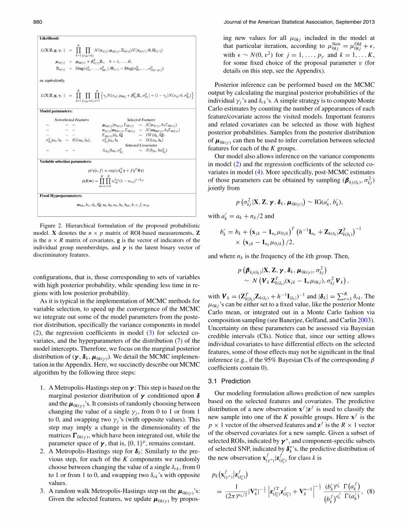
Figure 2 summarizes the hierarchical formulation of our fullmodel.

3. POSTERIOR INFERENCE

For posterior inference, our primary interest is in the selectionof the discriminating features and of the covariates that affectthe observed measurements, as captured by the selection vec-tors γγγ and δδδ. We also want to do inference on the dependencestructure among the selected features. Here we design a MCMCalgorithm that explores the model space for configurations withhigh posterior probability. These algorithms are commonly usedin Bayesian variable selection settings, and have been success-fully employed in genomic applications with very large num-ber of variables (George and McCulloch 1993, 1997; Brown,Vannucci, and Fearn 1998; Tadesse, Sha, and Vannucci 2005;Stingo et al. 2011). Clearly, with large dimensions, exploring theposterior space is a challenging problem. A typical strategy re-lies on exploiting the sparsity of the model, that is, the belief thatmost of the variables are not related to the underlying biologi-cal process. Such algorithm allows then to explore the posteriorspace in an effective way, quickly finding the most probable

880 Journal of the American Statistical Association, September 2013

Figure 2. Hierarchical formulation of the proposed probabilisticmodel. X denotes the n × p matrix of ROI-based measurements, Zis the n × R matrix of covariates, g is the vector of indicators of theindividual group memberships, and γ is the latent binary vector ofdiscriminatory features.

configurations, that is, those corresponding to sets of variableswith high posterior probability, while spending less time in re-gions with low posterior probability.

As it is typical in the implementation of MCMC methods forvariable selection, to speed up the convergence of the MCMCwe integrate out some of the model parameters from the poste-rior distribution, specifically the variance components in model(2), the regression coefficients in model (3) for selected co-variates, and the hyperparameters of the distribution (7) of themodel intercepts. Therefore, we focus on the marginal posteriordistribution of (γγγ , δδδk , µµµ0k(γ )). We detail the MCMC implemen-tation in the Appendix. Here, we succinctly describe our MCMCalgorithm by the following three steps:

1. A Metropolis-Hastings step on γγγ : This step is based on themarginal posterior distribution of γγγ conditioned upon δδδ

and the µµµ0k(γ )’s. It consists of randomly choosing betweenchanging the value of a single γj , from 0 to 1 or from 1to 0, and swapping two γj ’s (with opposite values). Thisstep may imply a change in the dimensionality of thematrices )))0k(γ ), which have been integrated out, while theparameter space of γγγ , that is, {0, 1}p, remains constant.

2. A Metropolis-Hastings step for δδδk: Similarly to the pre-vious step, for each of the K components we randomlychoose between changing the value of a single δrk , from 0to 1 or from 1 to 0, and swapping two δrk’s with oppositevalues.

3. A random walk Metropolis-Hastings step on the µµµ0k(γ )’s:Given the selected features, we update µµµ0k(γ ) by propos-

ing new values for all µ0kj included in the model atthat particular iteration, according to µNew

0kj = µOld0kj + ϵ,

with ϵ ∼ N (0, v2) for j = 1, . . . , pγ and k = 1, . . . K ,for some fixed choice of the proposal parameter v (fordetails on this step, see the Appendix).

Posterior inference can be performed based on the MCMCoutput by calculating the marginal posterior probabilities of theindividual γj ’s and δrk’s. A simple strategy is to compute MonteCarlo estimates by counting the number of appearances of eachfeature/covariate across the visited models. Important featuresand related covariates can be selected as those with highestposterior probabilities. Samples from the posterior distributionof µµµ0k(γ ) can then be used to infer correlation between selectedfeatures for each of the K groups.

Our model also allows inference on the variance componentsin model (2) and the regression coefficients of the selected co-variates in model (4). More specifically, post-MCMC estimatesof those parameters can be obtained by sampling (βββkj (δk), σ

2kj )

jointly from

p(σ 2

kj |X, Z, γγγ , δδδk, µµµ0k(γ ))

∼ IG(a′k, b

′k),

with a′k = ak + nk/2 and

b′k = bk +

(xjk − 1nk

µ0jk

)T (h−1Ink

+ Zk(δk)ZTk(δk)

)−1

×(xjk − 1nk

µ0jk

)/2,

and where nk is the frequency of the kth group. Then,

p(βββkj (δk)|X, Z, γγγ , δδδk, µµµ0k(γ ), σ

2kj

)

∼ N(VVV k ZT

k(δk)(xjk − 1nµ0kj ), σ 2kjVVV k

),

with VVV k = (ZTk(δk)Zk(δk) + h−1I|δk |)

−1 and |δδδk| =∑R

r=1 δrk . Theµ0kj ’s can be either set to a fixed value, like the posterior MonteCarlo mean, or integrated out in a Monte Carlo fashion viacomposition sampling (see Banerjee, Gelfand, and Carlin 2003).Uncertainty on these parameters can be assessed via Bayesiancredible intervals (CIs). Notice that, since our setting allowsindividual covariates to have differential effects on the selectedfeatures, some of those effects may not be significant in the finalinference (e.g., if the 95% Bayesian CIs of the corresponding β

coefficients contain 0).

3.1 Prediction

Our modeling formulation allows prediction of new samplesbased on the selected features and covariates. The predictivedistribution of a new observation xf |zf is used to classify thenew sample into one of the K possible groups. Here xf is thep × 1 vector of the observed features and zf is the R × 1 vectorof the observed covariates for a new sample. Given a subset ofselected ROIs, indicated by γγγ ∗, and component-specific subsetsof selected SNP, indicated by δδδ∗

k’s, the predictive distribution ofthe new observation xf

(γ ∗)|zf(δ∗

k ) for class k is

pk

(xf

(γ ∗)

∣∣zf(δ∗

k )

)

= 1(2π )nk/2

|V∗k |−

12

∣∣∣zf T(δ∗

k )zf(δ∗

k ) + V∗−1k

∣∣∣− 1

2 (b′k)a

′k

(b

fk

)afk

)(a

fk

)

)(a′k)

, (8)

Stingo et al.: Bayesian Modeling Approach to Imaging Genetics 881

where

afk = a′

k + 1/2,

V∗k =

(ZT

k(δ∗k )Zk(δ∗

k ) + h−1I|δk |)−1

,

bfk = bk + (xjk(γ ∗) − 1nk

µ0jk)T Zk(δ∗k )V∗

k

×(V−1

k − V−1k

(ZT

k(δ∗k )Zk(δ∗

k ) + V−1k

)−1V−1k

)

× V∗kZT

k(δ∗k )

(xjk(γ ∗) − 1nk

µ0jk

)/2 +

(xf

jk(γ ∗) − µ0jk

)2

2(1 + zf

(δ∗k )Vkzf T

(δ∗k )

) .

In model (8) the µ0kj ’s are assumed to be set to a fixedvalue, for example the posterior Monte Carlo mean or median.Alternatively, one can perform a Monte Carlo integration of theµ0kj ’s using the values sampled within the MCMC algorithm. Inour experience, we have not noticed any significant differencebetween the two approaches.

The probability that a future observation, given the observeddata, belongs to the group k is then

πk(gf |X, Z) = p(gf = k|xf , X, zf , Z),

where gf is the group indicator of the new observation. Byestimating the probability πk = P (gi = k) that one observationcomes from group k as πk = nk/n, the previous distribution canbe written in closed form as

πg(gf |X, Z) =pk

(xf

(γ ∗)

∣∣zf(δ∗

k )

)πk

∑Ki=1 pi

(xf

(γ ∗)

∣∣zf(δ∗

k )

)πi

, (9)

with pk(xf(γ ∗)|z

f(δ∗

k )) the predictive distribution defined in model(8), and the new sample can be classified based on this distri-bution, for example by assigning it to the group that has thehighest posterior probability. The plug-in estimate πk = nk/n

can be formally justified as an approximation under a nonin-formative Dirichlet prior distribution for π and training dataexchangeable with future data, meaning that observations fromtraining and validation sets arise in the same proportions fromthe groups (see e.g., Fearn, Brown, and Besbeas 2002).

4. APPLICATIONS

4.1 Simulation Studies

We investigate the performance of our model using simulateddata. We consider simulated scenarios mimicking the charac-teristics of the real data that motivated the development of themodel, where some of the ROIs appear to be highly correlated.We focus on situations where most of the measurements arenoisy and test the ability of our method to discover relevantfeatures in the presence of a large amount of noise. The SNPdata record the number of copies of the minor allele at eachlocus for each individual, as a sequence of {0,1,2} values indi-cating the three possible genotypes at each SNP: major allelehomozygote, heterozygote, and minor allele homozygote (seee.g., Servin and Stephens 2007, for a description of this addi-tive coding). In our simulations, we considered the same datasetused in the experimental data described in Section 4.2. Thischoice was made to preserve realistic patterns of correlation(also known as “linkage disequilibrium”) across multiple SNPs.The simulation comprised a total of R = 50 covariates (SNP),

only two of which were used to generate the measurements(activation profiles), as described below.

We generated a sample of 200 observations from a mixture ofK = 2 multivariate normal densities, induced by four variables(features), as

xi ∼ I[1≤i≤n1]N4(µµµ01 + BT

1 Zi ,%%%1)

+ I[n1<i≤200]N4(µµµ02 + BT

2 Zi ,%%%2),

with xi = (xi1, . . . , xi4)T , for i = 1, . . . , 200, and where I[.] isthe indicator function. The first n1 = 150 samples were from thefirst component of the mixture, the last n2 = 50 from the second.We then randomly divided the samples into a training set of 100observations and a validation set of the same size. We set theelements of the 4 × 1 vector µµµ01 to 0.8 and those of µµµ02 to −0.8.The (2 × 4) regression coefficient matrix Bk = (βββk1, . . . , βββk4)determines the effects of the true covariates on the simulatedactivation profiles. We set B1 = 0.8 · 12×4 and B2 = 0.8 · 12×4.The covariance structure among the relevant features was chosenby setting the off-diagonal elements of %%%1 and %%%2 to 0.5 whereasthe diagonal elements were set to 1. Note that the data-generatingprocess differs from our proposed model, where the correlationstructure among the features is modeled at a hidden level via thebaseline component. In addition to the four relevant features, wegenerated 100 noisy ones from a multivariate normal distributioncentered at zero, with variances equal to 1 and off-diagonalelements of the covariance matrix equal to 0.1.

Our simulation comprises a total of 104 features and 50 co-variates. We aim at finding the four discriminating features andthe two covariates that truly relate to the response measurements.We are also interested in capturing the correlation structureamong selected features. Our full prior model and the relatedhyperparameters are summarized in Figure 1. We report theresults obtained by choosing, when possible, hyperparametersthat lead to weakly informative prior distributions. In particular,we specified the priors on σ 2

0j and σ 2kj by setting a0 = ak = 3,

the minimum integer value such that the variance is defined,and b0 = bk = 0.1. Using the same rationale, we set dk = 3,the minimum value such that the expectation of %%%k exists, andQ = c Ip with c = 0.1. As for the β vectors of regression co-efficients, we set the prior mean to b01 = b02 = 0. Similarly,we set m10 = m20 = 0. We then set h to 4 and h1 to 1, to ob-tain fairly flat priors over the region where the data are defined;larger values of these hyperparameters would encourage the se-lection of only very large effects whereas smaller values wouldencourage the selection of smaller effects. As for the featureselection indicator, γγγ , we set e = −3, which corresponds tosetting the expected proportion of features a priori included inthe model to 5% of the total number of available ones. In thissimulation study, we did not use any network structure on theprior distribution of γγγ , which correspond to set f = 0. This isalso equivalent to assuming p(γγγ ) as a product of independentBernoulli distributions with expected value equal to 0.05. Fi-nally, regarding the prior on the covariate selection indicator δδδ,we set wrk = 0.05, which corresponds to setting the proportionof covariates expected a priori in the model to 5%. Parameterse and wr influence the sparsity of the model.

We ran three MCMC samplers for 30,000 iterations with thefirst 1000 discarded as burn-in. As starting points of the chain,

882 Journal of the American Statistical Association, September 2013

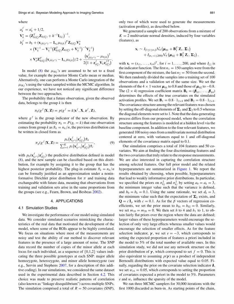
Figure 3. Simulation study: marginal posterior probabilities of inclusion for features (left) and covariates (middle and right).

we considered three different pairs of discriminatory ROIsand significant SNPs. More specifically, we assumed differentstarting counts of included ROIs and SNPs, that is, 2 ROIs and2 SNPs, 10 ROIs and 5 SNPs, and 15 ROIs and 10 SNPs, re-spectively. The actual ROIs and SNPs initially included wererandomly selected from the set of available features and co-variates. To assess the agreement of the results between thetwo chains, we looked at the correlation between the marginalposterior probabilities for ROI selection, p(γj |Z, X), and SNPselection, p(δlk|Z, X) for k = 1, 2. These indicated good con-cordance between the three MCMC chains, with pairwise cor-relation coefficients ranging from 0.999 to 1 for ROIs and from0.997 to 0.998 (k = 1) and from 0.993 to 0.999 (k = 2) forSNPs. Concordance among the marginal posterior probabilitieswas confirmed by looking at scatterplots of the marginal prob-abilities across each pair of MCMC chains (figures not shown).We also used the Gelman and Rubin’s convergence diagnostics(Gelman and Rubin 1992) to assess the convergence of the pa-rameters µ0kj ’s to their posterior distributions. Those statisticswere all below 1.1, ranging from 1.0051 to 1.0212, clearly indi-cating that the MCMC chains were run for a satisfactory numberof iterations.

We then computed marginal posterior probabilities for featureand covariate selection, p(γj = 1|Z, X) and p(δrk = 1|Z, X),respectively. These are displayed in Figure 3, for all 104 fea-tures and the 50 covariates. All four relevant features were cor-rectly identified by our model, with high posterior probability(> 0.98), while noisy features showed posterior probabilitiessmaller than 1%. In addition, the two relevant covariates werealso selected for the first group, with p(δr1 = 1|Z, X) > 0.92,and one relevant covariate was selected for the second group,with p(δr2 = 1|Z, X) > 0.99. Sensitivity analyses with differ-ent choices of e and wrk indicated that the posterior inference isquite robust. Specifically, our selection results were practicallyinvariant when we let e vary between −3.5 and −2, which isequivalent to an a priori expected proportion of included fea-tures between 3% and roughly 10%, and wrk vary between 3%and 10%. Regarding the other hyperparameters of the model, wenoticed that smaller values of h would encourage the inclusion

of smaller effects and that setting this parameter to 1 would leadto the inclusion of a few false positive covariates.

Posterior distributions of the intercept parameters µµµ01 andµµµ02, given the selected features, indicated that parameters char-acterizing the two groups are clearly different. For example,Figure 4 shows the posterior distributions of the elements µ011

and µ021, corresponding to the first selected feature. These dis-tributions were obtained from the MCMC output conditioningupon the inclusion of the four relevant features. Similar plotswere obtained for other selected features (not shown).

We estimated the dependence structure among selected fea-tures by looking at the posterior correlations among the corre-sponding intercepts, calculated based on the MCMC samples.These were

Corrµµµ01=

⎛

⎜⎜⎜⎝

1.0000 0.5480 0.5916 0.4426

0.5480 1.0000 0.6075 0.4848

0.5916 0.6075 1.0000 0.4930

0.4426 0.4848 0.4930 1.0000

⎞

⎟⎟⎟⎠

and

Corrµµµ02=

⎛

⎜⎜⎜⎝

1.0000 0.5322 0.5740 0.5379

0.5322 1.0000 0.5075 0.4535

0.5740 0.5075 1.0000 0.4924

0.5379 0.4535 0.4924 1.0000

⎞

⎟⎟⎟⎠

for Groups 1 and 2, respectively. These estimates show that ourmodel is indeed able to capture correlation structure among se-lected features. Furthermore, we summarized the distance of theestimated correlation matrices from the true ones using the RV-coefficient, a measure of similarity between positive semidefi-nite matrices (Robert and Escoufier 1976; Smilde et al. 2009).The RV coefficient RV ∈ (0, 1) may be considered as a gen-eralization of the Pearson’s coefficient of determination. Forboth Groups 1 and 2, we got values very close to 1, that is,RV = 0.994 for Corrµµµ01

and RV = 0.997 for Corrµµµ02, suggest-

ing good agreement with the true correlation structures.Finally, we assessed predictive performance. We used the four

selected features and the three selected covariates, 2 for the first

Stingo et al.: Bayesian Modeling Approach to Imaging Genetics 883

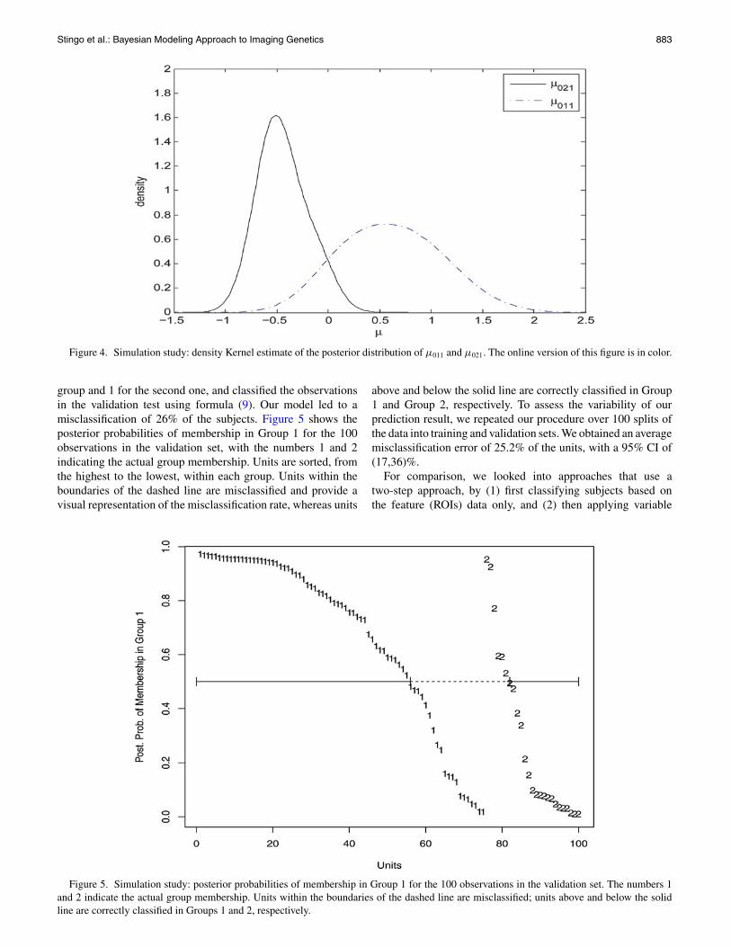
Figure 4. Simulation study: density Kernel estimate of the posterior distribution of µ011 and µ021. The online version of this figure is in color.

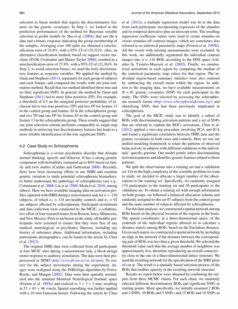
group and 1 for the second one, and classified the observationsin the validation test using formula (9). Our model led to amisclassification of 26% of the subjects. Figure 5 shows theposterior probabilities of membership in Group 1 for the 100observations in the validation set, with the numbers 1 and 2indicating the actual group membership. Units are sorted, fromthe highest to the lowest, within each group. Units within theboundaries of the dashed line are misclassified and provide avisual representation of the misclassification rate, whereas units

above and below the solid line are correctly classified in Group1 and Group 2, respectively. To assess the variability of ourprediction result, we repeated our procedure over 100 splits ofthe data into training and validation sets. We obtained an averagemisclassification error of 25.2% of the units, with a 95% CI of(17,36)%.

For comparison, we looked into approaches that use atwo-step approach, by (1) first classifying subjects based onthe feature (ROIs) data only, and (2) then applying variable

Figure 5. Simulation study: posterior probabilities of membership in Group 1 for the 100 observations in the validation set. The numbers 1and 2 indicate the actual group membership. Units within the boundaries of the dashed line are misclassified; units above and below the solidline are correctly classified in Groups 1 and 2, respectively.

884 Journal of the American Statistical Association, September 2013

selection in linear models that regress the discriminatory fea-tures on the genetic covariates. In Step 1, we looked at theprediction performances of the method for Bayesian variableselection in probit models by Sha et al. (2004), that use the xdata and a binary response indicating the group membership ofthe samples. Averaging over 100 splits we obtained a misclas-sification error of 24.8%, with a 95% CI of (19,32)%. Also, analternative classification method, based on support vector ma-chine (SVM; Cristianini and Shawe-Taylor 2000), resulted in amisclassification error of 27.8%, with a 95% CI of (21,36)%. InStep 2, to avoid selection biases, we used the truly discrimina-tory features as response variables. We applied the method byGuan and Stephens (2011), separately for each group of subjectsand each feature, and compared the results with our joint esti-mation method. Recall that our method identified three true andno false significant SNPs. In general, the method by Guan andStephens (2011) led to more false positives (FP). For example,a threshold of 0.5 on the marginal posterior probability of in-clusion led to two true positives (TP) and two FP for feature 13in the control group and feature 20 in the schizophrenia group,and two TP and one FP for feature 83 in the control group andfeature 13 in the schizophrenia group. These results suggest thatour joint selection scheme performs comparably to single-stepmethods in retrieving true discriminatory features but leads to amore reliable identification of the true significant SNPs.

4.2 Case Study on Schizophrenia

Schizophrenia is a severe psychiatric disorder that disruptsnormal thinking, speech, and behavior. It has a strong geneticcomponent with heritability estimated up to 80% based on fam-ily and twin studies (Cardno and Gottesman 2000). Recently,there have been increasing efforts to use fMRI and examinegenetic variation to study potential schizophrenia biomarkers,to better understand the pathology of schizophrenia (see e.g.,Colantuoni et al. 2008; Liu et al. 2009; Meda et al. 2010, amongothers). Here we have available imaging data on activation pro-files captured with fMRI during a sensorimotor task for n = 210subjects, of which n1 = 118 are healthy controls and n2 = 92are subjects affected by schizophrenia. Participant recruitmentand data collection were conducted by the MCIC, a collabora-tive effort of four research teams from Boston, Iowa, Minnesota,and New Mexico. Prior to inclusion in the study, all healthy par-ticipants were screened to ensure that they were free of anymedical, neurological, or psychiatric illnesses, including anyhistory of substance abuse. Additional information, includingparticipants demographics, can be found in the article by Chenet al. (2012).

The original fMRI data were collected from all participantsat four MCIC sites during a sensorimotor task, a block-designmotor response to auditory stimulation. The data were then pre-processed in SPM5 (http://www.fil.ion.ucl.ac.uk/spm). To cor-rect for the subject movements during the experiment, im-ages were realigned using the INRIAlign algorithm by Freire,Roche, and Mangin (2002). Data were then spatially normal-ized into the standard Montreal Neurological Institute space(Friston et al. 1995a) and resliced to 3 × 3 × 3 mm, resultingin 53 × 63 × 46 voxels. Spatial smoothing was further appliedwith a 10 mm Gaussian kernel. Following the article by Chen

et al. (2012), a multiple regression model was fit to the datafrom each participant, incorporating regressors of the stimulusand its temporal derivative plus an intercept term. The resultingregression coefficient values were used to create stimulus-onversus stimulus-off contrast images, which are sometimes alsoreferred to as statistical parametric maps (Friston et al. 1995b).All the voxels with missing measurements were excluded. Inthis work, we additionally segmented the individual contrastimages into p = 116 ROIs according to the MNI space AALatlas by Tzourio-Mazoyer et al. (2002). Finally, we summa-rized activations in each region by computing the median ofthe statistical parametric map values for that region. The in-dividual region-based summary statistics were also centeredby subtracting the overall mean within the region. In addi-tion to the imaging data, we have available measurements onR = 81 genetic covariates (SNP) for each participant in thestudy. The SNPs were selected by accessing the schizophre-nia research forum (http://www.schizophreniaforum.org/) andidentifying SNPs that had been previously implicated inschizophrenia.

The goal of the MCIC study was to identify a subset ofROIs with discriminating activation patterns and a set of SNPsthat are relevant to explain the ROI’s activations. Chen et al.(2012) applied a two-step procedure involving PCA and ICAand found a significant correlation between fMRI data and thegenetic covariates in both cases and controls. Here we use ourunified modeling framework to relate the patterns of observedbrain activity in subjects with different conditions to the individ-uals’ specific genome. Our model jointly infers discriminatingactivation patterns and identifies genetic features related to thosepatterns.

We split the observations into a training set and a validationset. Given the high complexity of the scientific problem we wantto study, we decided to allocate a larger number of the obser-vations to the training set. Specifically, we randomly assigned174 participants to the training set and 36 participants to thevalidation set. To obtain a training set with enough informationon both groups, we followed a balanced allocation scheme andrandomly assigned to this set 87 subjects from the control groupand the same number of subjects affected by schizophrenia.

For this data analysis, we constructed a spatial network amongROIs based on the physical location of the regions in the brain.The spatial coordinates, in a three-dimensional space, of thecentroids of the individual regions allowed us to calculate adistance matrix among ROIs, based on the Euclidean distance.Given such matrix we constructed a spatial network by includingan edge in the network if the distance between the correspond-ing pair of ROIs was less than a given threshold. We selected thethreshold value such that the average number of neighbors wasapproximately five, therefore reproducing an overall connectiv-ity close to the one of a three-dimensional lattice structure. Weused the resulting network for the specification of the MRF prior(6) on γγγ . The result is a spatially based selection process of theROIs that enables sparsity in the resulting network structure.

Results we report below were obtained by combining the out-puts from three MCMC chains. For each chain, we randomlyselected different discriminatory ROIs and significant SNPs asstarting points. More specifically, we initially assumed 2 ROIsand 2 SNPs, 10 ROIs and 5 SNPs, and 15 ROIs and 10 SNPs as

Stingo et al.: Bayesian Modeling Approach to Imaging Genetics 885

0 20 40 60 80 100 120

0.0

0.2

0.4

0.6

0.8

1.0

ROIs − f=0.1 (circle) and 0.5 (cross)

Pos

terio

r P

roba

bilit

y of

Incl

usio

n

●●●●

●

●●●●●●●●●●●●●●●

●●

●●●●

●

●

●●●●●●●●●●●●●●●●●●●●●●●●●●●●●●●●●●●●●●●●●●●●●●●●●●●●●●●●●●

●

●●●●●●●●●●●●●●●●●●●●●●●●●●●●●

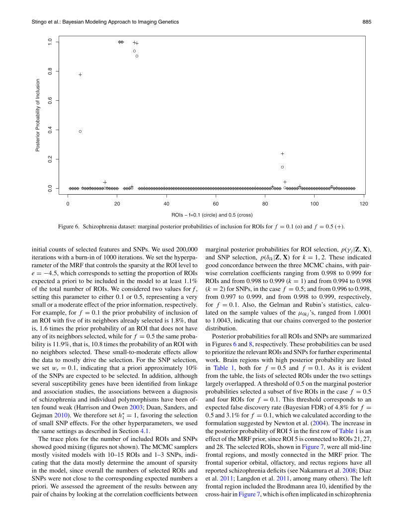
Figure 6. Schizophrenia dataset: marginal posterior probabilities of inclusion for ROIs for f = 0.1 (o) and f = 0.5 (+).

initial counts of selected features and SNPs. We used 200,000iterations with a burn-in of 1000 iterations. We set the hyperpa-rameter of the MRF that controls the sparsity at the ROI level toe = −4.5, which corresponds to setting the proportion of ROIsexpected a priori to be included in the model to at least 1.1%of the total number of ROIs. We considered two values for f ,setting this parameter to either 0.1 or 0.5, representing a verysmall or a moderate effect of the prior information, respectively.For example, for f = 0.1 the prior probability of inclusion ofan ROI with five of its neighbors already selected is 1.8%, thatis, 1.6 times the prior probability of an ROI that does not haveany of its neighbors selected, while for f = 0.5 the same proba-bility is 11.9%, that is, 10.8 times the probability of an ROI withno neighbors selected. These small-to-moderate effects allowthe data to mostly drive the selection. For the SNP selection,we set wr = 0.1, indicating that a priori approximately 10%of the SNPs are expected to be selected. In addition, althoughseveral susceptibility genes have been identified from linkageand association studies, the associations between a diagnosisof schizophrenia and individual polymorphisms have been of-ten found weak (Harrison and Owen 2003; Duan, Sanders, andGejman 2010). We therefore set h∗

1 = 1, favoring the selectionof small SNP effects. For the other hyperparameters, we usedthe same settings as described in Section 4.1.

The trace plots for the number of included ROIs and SNPsshowed good mixing (figures not shown). The MCMC samplersmostly visited models with 10–15 ROIs and 1–3 SNPs, indi-cating that the data mostly determine the amount of sparsityin the model, since overall the numbers of selected ROIs andSNPs were not close to the corresponding expected numbers apriori. We assessed the agreement of the results between anypair of chains by looking at the correlation coefficients between

marginal posterior probabilities for ROI selection, p(γj |Z, X),and SNP selection, p(δlk|Z, X) for k = 1, 2. These indicatedgood concordance between the three MCMC chains, with pair-wise correlation coefficients ranging from 0.998 to 0.999 forROIs and from 0.998 to 0.999 (k = 1) and from 0.994 to 0.998(k = 2) for SNPs, in the case f = 0.5; and from 0.996 to 0.998,from 0.997 to 0.999, and from 0.998 to 0.999, respectively,for f = 0.1. Also, the Gelman and Rubin’s statistics, calcu-lated on the sample values of the µ0kj ’s, ranged from 1.0001to 1.0043, indicating that our chains converged to the posteriordistribution.

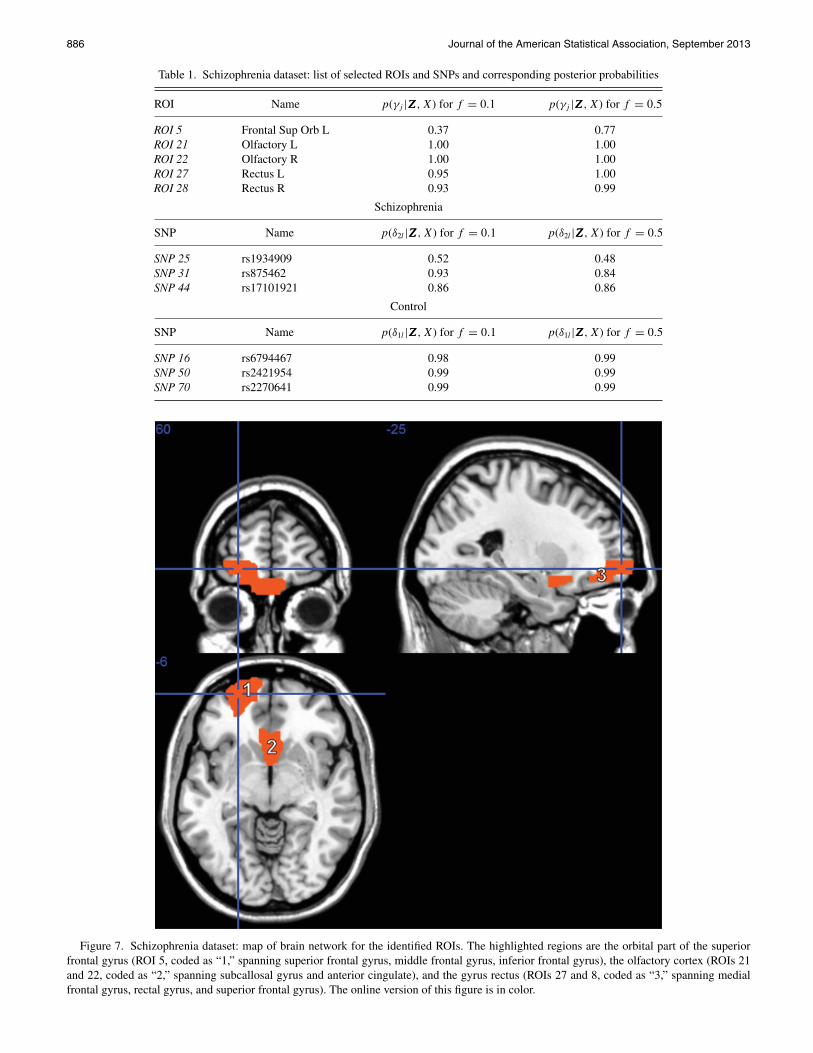
Posterior probabilities for all ROIs and SNPs are summarizedin Figures 6 and 8, respectively. These probabilities can be usedto prioritize the relevant ROIs and SNPs for further experimentalwork. Brain regions with high posterior probability are listedin Table 1, both for f = 0.5 and f = 0.1. As it is evidentfrom the table, the lists of selected ROIs under the two settingslargely overlapped. A threshold of 0.5 on the marginal posteriorprobabilities selected a subset of five ROIs in the case f = 0.5and four ROIs for f = 0.1. This threshold corresponds to anexpected false discovery rate (Bayesian FDR) of 4.8% for f =0.5 and 3.1% for f = 0.1, which we calculated according to theformulation suggested by Newton et al. (2004). The increase inthe posterior probability of ROI 5 in the first row of Table 1 is aneffect of the MRF prior, since ROI 5 is connected to ROIs 21, 27,and 28. The selected ROIs, shown in Figure 7, were all mid-linefrontal regions, and mostly connected in the MRF prior. Thefrontal superior orbital, olfactory, and rectus regions have allreported schizophrenia deficits (see Nakamura et al. 2008; Diazet al. 2011; Langdon et al. 2011, among many others). The leftfrontal region included the Brodmann area 10, identified by thecross-hair in Figure 7, which is often implicated in schizophrenia

886 Journal of the American Statistical Association, September 2013

Table 1. Schizophrenia dataset: list of selected ROIs and SNPs and corresponding posterior probabilities

ROI Name p(γj |ZZZ, X) for f = 0.1 p(γj |ZZZ,X) for f = 0.5

ROI 5 Frontal Sup Orb L 0.37 0.77ROI 21 Olfactory L 1.00 1.00ROI 22 Olfactory R 1.00 1.00ROI 27 Rectus L 0.95 1.00ROI 28 Rectus R 0.93 0.99

Schizophrenia

SNP Name p(δ2l |ZZZ,X) for f = 0.1 p(δ2l |ZZZ, X) for f = 0.5

SNP 25 rs1934909 0.52 0.48SNP 31 rs875462 0.93 0.84SNP 44 rs17101921 0.86 0.86

Control

SNP Name p(δ1l |ZZZ,X) for f = 0.1 p(δ1l |ZZZ, X) for f = 0.5

SNP 16 rs6794467 0.98 0.99SNP 50 rs2421954 0.99 0.99SNP 70 rs2270641 0.99 0.99

Figure 7. Schizophrenia dataset: map of brain network for the identified ROIs. The highlighted regions are the orbital part of the superiorfrontal gyrus (ROI 5, coded as “1,” spanning superior frontal gyrus, middle frontal gyrus, inferior frontal gyrus), the olfactory cortex (ROIs 21and 22, coded as “2,” spanning subcallosal gyrus and anterior cingulate), and the gyrus rectus (ROIs 27 and 8, coded as “3,” spanning medialfrontal gyrus, rectal gyrus, and superior frontal gyrus). The online version of this figure is in color.

Stingo et al.: Bayesian Modeling Approach to Imaging Genetics 887

0 20 40 60 80

0.0

0.2

0.4

0.6

0.8

1.0

SNPs − f=0.1 (circle) and 0.5 (cross)

Pos

terio

r P

roba

bilit

y of

Incl

usio

nControl group

0 20 40 60 80

0.0

0.2

0.4

0.6

0.8

1.0

SNPs − f=0.1 (circle) and 0.5 (cross)P

oste

rior

Pro

babi

lity

of In

clus

ion

Schizophrenia group

Figure 8. Schizophrenia dataset: marginal posterior probabilities of inclusion for SNPs for f = 0.1 (o) and f = 0.5 (+).

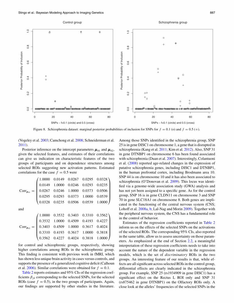
(Vogeley et al. 2003; Camchong et al. 2008; Schneiderman et al.2011).

Posterior inference on the intercept parameters µµµ01 and µµµ02,given the selected features, and estimates of their correlationscan give us indication on characteristic features of the twogroups of participants and on dependence structures amongselected ROIs suggesting new activation patterns. Estimatedcorrelations for the case f = 0.5 were

Corrµ01 =

⎛

⎜⎜⎜⎜⎜⎜⎝

1.0000 0.0149 0.0267 0.0295 0.0328

0.0149 1.0000 0.0246 0.0293 0.0235

0.0267 0.0246 1.0000 0.0373 0.0506

0.0295 0.0293 0.0373 1.0000 0.0539

0.0328 0.0235 0.0506 0.0539 1.0000

⎞

⎟⎟⎟⎟⎟⎟⎠

and

Corrµ02 =

⎛

⎜⎜⎜⎜⎜⎜⎝

1.0000 0.3532 0.3403 0.3310 0.3562

0.3532 1.0000 0.4509 0.4193 0.4227

0.3403 0.4509 1.0000 0.3617 0.4024

0.3310 0.4193 0.3617 1.0000 0.3818

0.3562 0.4227 0.4024 0.3818 1.0000

⎞

⎟⎟⎟⎟⎟⎟⎠

for control and schizophrenic groups, respectively, showinghigher correlations among ROIs in the schizophrenic group.This finding is consistent with previous work in fMRI, whichhas shown less unique brain activity in cases versus controls, andsupports the presence of a generalized cognitive deficit (Calhounet al. 2006). Similar correlations were obtained for f = 0.1.

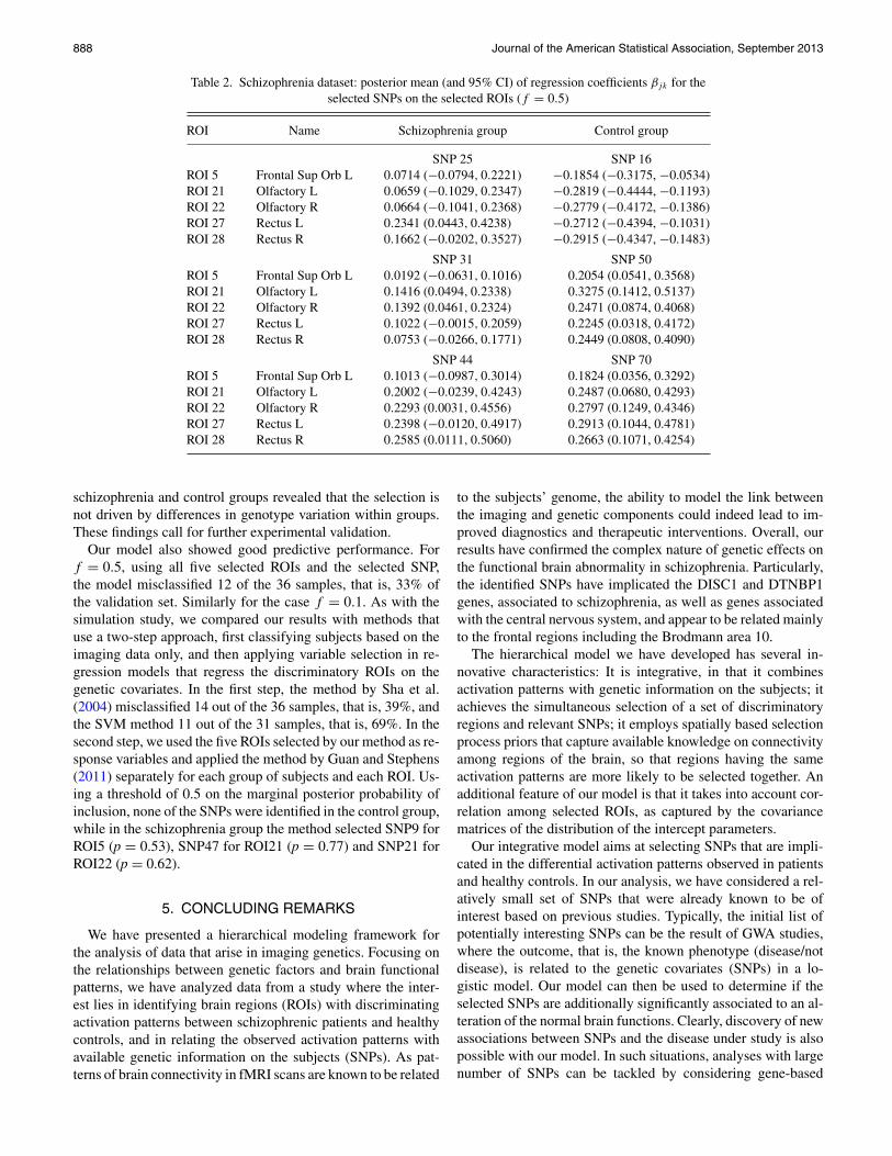
Table 2 reports estimates and 95% CIs of the regression coef-ficients βjk corresponding to the selected SNPs, for the selectedROIs (case f = 0.5), in the two groups of participants. Again,our findings are supported by other studies in the literature.

Among those SNPs identified in the schizophrenia group, SNP25 is in gene DISC1 on chromosome 1, a gene that is disrupted inschizophrenia (Kang et al. 2011; Kim et al. 2012). Also, SNP 31in gene DTNBP1 on chromosome 6 has been found associatedwith schizophrenia (Duan et al. 2007). Interestingly, Colantuoniet al. (2008) reported age-related changes in the expression ofputative schizophrenia genes, including DISC1 and DTNBP1,in the human prefrontal cortex, including Brodmann area 10.SNP 44 is on chromosome 10 and it has also been associated toschizophrenia (O’Donovan et al. 2009). This locus was identi-fied via a genome-wide association study (GWA) analysis andhas not yet been assigned to a specific gene. As for the controlgroup, SNP 16 is in gene CLDN11 on chromosome 3 and SNP70 in gene SLC18A1 on chromosome 8. Both genes are impli-cated in the functioning of the central nervous system (CNS;Lohoff et al. 2008a, b; Lal-Nag and Morin 2009). Together withthe peripheral nervous system, the CNS has a fundamental rolein the control of behavior.

Estimates of the regression coefficients reported in Table 2inform us on the effects of the selected SNPs on the activationsof the selected ROIs. The corresponding 95% CIs, also reportedin the same table, allow us to assess uncertainty on those param-eters. As emphasized at the end of Section 2.2, a meaningfulinterpretation of these regression coefficients needs to take intoaccount the nature of the dependent variable in the regressionmodels, which is the set of discriminatory ROIs in the twogroups. An interesting feature of our results is that, while ef-fects are all significant across selected ROIs in the control group,differential effects are clearly indicated in the schizophreniagroup. For example, SNP 25 (rs1934909 in gene DISC1) has asignificant effect on the Rectus L ROI only and SNP 31(rs875462 in gene DTNBP1) on the Olfactory ROIs only. Aclose look at the alleles’ frequencies of the selected SNPs in the

888 Journal of the American Statistical Association, September 2013

Table 2. Schizophrenia dataset: posterior mean (and 95% CI) of regression coefficients βjk for theselected SNPs on the selected ROIs (f = 0.5)

ROI Name Schizophrenia group Control group

SNP 25 SNP 16ROI 5 Frontal Sup Orb L 0.0714 (−0.0794, 0.2221) −0.1854 (−0.3175, −0.0534)ROI 21 Olfactory L 0.0659 (−0.1029, 0.2347) −0.2819 (−0.4444, −0.1193)ROI 22 Olfactory R 0.0664 (−0.1041, 0.2368) −0.2779 (−0.4172, −0.1386)ROI 27 Rectus L 0.2341 (0.0443, 0.4238) −0.2712 (−0.4394, −0.1031)ROI 28 Rectus R 0.1662 (−0.0202, 0.3527) −0.2915 (−0.4347, −0.1483)

SNP 31 SNP 50ROI 5 Frontal Sup Orb L 0.0192 (−0.0631, 0.1016) 0.2054 (0.0541, 0.3568)ROI 21 Olfactory L 0.1416 (0.0494, 0.2338) 0.3275 (0.1412, 0.5137)ROI 22 Olfactory R 0.1392 (0.0461, 0.2324) 0.2471 (0.0874, 0.4068)ROI 27 Rectus L 0.1022 (−0.0015, 0.2059) 0.2245 (0.0318, 0.4172)ROI 28 Rectus R 0.0753 (−0.0266, 0.1771) 0.2449 (0.0808, 0.4090)

SNP 44 SNP 70ROI 5 Frontal Sup Orb L 0.1013 (−0.0987, 0.3014) 0.1824 (0.0356, 0.3292)ROI 21 Olfactory L 0.2002 (−0.0239, 0.4243) 0.2487 (0.0680, 0.4293)ROI 22 Olfactory R 0.2293 (0.0031, 0.4556) 0.2797 (0.1249, 0.4346)ROI 27 Rectus L 0.2398 (−0.0120, 0.4917) 0.2913 (0.1044, 0.4781)ROI 28 Rectus R 0.2585 (0.0111, 0.5060) 0.2663 (0.1071, 0.4254)

schizophrenia and control groups revealed that the selection isnot driven by differences in genotype variation within groups.These findings call for further experimental validation.

Our model also showed good predictive performance. Forf = 0.5, using all five selected ROIs and the selected SNP,the model misclassified 12 of the 36 samples, that is, 33% ofthe validation set. Similarly for the case f = 0.1. As with thesimulation study, we compared our results with methods thatuse a two-step approach, first classifying subjects based on theimaging data only, and then applying variable selection in re-gression models that regress the discriminatory ROIs on thegenetic covariates. In the first step, the method by Sha et al.(2004) misclassified 14 out of the 36 samples, that is, 39%, andthe SVM method 11 out of the 31 samples, that is, 69%. In thesecond step, we used the five ROIs selected by our method as re-sponse variables and applied the method by Guan and Stephens(2011) separately for each group of subjects and each ROI. Us-ing a threshold of 0.5 on the marginal posterior probability ofinclusion, none of the SNPs were identified in the control group,while in the schizophrenia group the method selected SNP9 forROI5 (p = 0.53), SNP47 for ROI21 (p = 0.77) and SNP21 forROI22 (p = 0.62).

5. CONCLUDING REMARKS

We have presented a hierarchical modeling framework forthe analysis of data that arise in imaging genetics. Focusing onthe relationships between genetic factors and brain functionalpatterns, we have analyzed data from a study where the inter-est lies in identifying brain regions (ROIs) with discriminatingactivation patterns between schizophrenic patients and healthycontrols, and in relating the observed activation patterns withavailable genetic information on the subjects (SNPs). As pat-terns of brain connectivity in fMRI scans are known to be related

to the subjects’ genome, the ability to model the link betweenthe imaging and genetic components could indeed lead to im-proved diagnostics and therapeutic interventions. Overall, ourresults have confirmed the complex nature of genetic effects onthe functional brain abnormality in schizophrenia. Particularly,the identified SNPs have implicated the DISC1 and DTNBP1genes, associated to schizophrenia, as well as genes associatedwith the central nervous system, and appear to be related mainlyto the frontal regions including the Brodmann area 10.

The hierarchical model we have developed has several in-novative characteristics: It is integrative, in that it combinesactivation patterns with genetic information on the subjects; itachieves the simultaneous selection of a set of discriminatoryregions and relevant SNPs; it employs spatially based selectionprocess priors that capture available knowledge on connectivityamong regions of the brain, so that regions having the sameactivation patterns are more likely to be selected together. Anadditional feature of our model is that it takes into account cor-relation among selected ROIs, as captured by the covariancematrices of the distribution of the intercept parameters.

Our integrative model aims at selecting SNPs that are impli-cated in the differential activation patterns observed in patientsand healthy controls. In our analysis, we have considered a rel-atively small set of SNPs that were already known to be ofinterest based on previous studies. Typically, the initial list ofpotentially interesting SNPs can be the result of GWA studies,where the outcome, that is, the known phenotype (disease/notdisease), is related to the genetic covariates (SNPs) in a lo-gistic model. Our model can then be used to determine if theselected SNPs are additionally significantly associated to an al-teration of the normal brain functions. Clearly, discovery of newassociations between SNPs and the disease under study is alsopossible with our model. In such situations, analyses with largenumber of SNPs can be tackled by considering gene-based

Stingo et al.: Bayesian Modeling Approach to Imaging Genetics 889

summaries of SNP data. Indeed, more and more GWA studiesconfirm the involvement of aggregates of common SNPs thatcollectively account for a substantial proportion of variation inrisk to the disorder (see Purcell et al. 2009, for a schizophreniastudy).

Several extensions of our model are worth investigating. First,we can learn about the fixed hyperparameters. For example, wecan assume prior distributions for the parameters of the Isingmodel, as in the articles by Liang (2010) and Stingo et al. (2011),as well as the scale parameters of the spike and slab priors (4), assometimes done in Bayesian variable selection (Chipman et al.2001; Scott and Berger 2010). Second, extensions to mixturemodels for clustering the subjects are possible. In particular, in-finite mixture models can be fit based on the Dirichlet process,as in the article by Kim, Tadesse, and Vannucci (2006), or basedon the probit stick-breaking process proposed by Chung andDunson (2009) for a mixture of univariate regression models,which also incorporates selection of the covariates. Furthermore,even though our method already suggests connections amongdistant features that can form new activation patterns, a moreformal approach could assume µµµ0k(γ ) to be a realization of a net-work of connected components (nodes) that describes generalrelationships among the selected features as

µµµ0k(γ )|Gk(γ ) ∼ Npγ(νννk(γ ),)))0k(γ )), k = 1, . . . , K, (10)

with Gk(γ ) the graph encoding the relationships (see Dobra,Lenkoski, and Rodriguez 2011). This would allow us to es-timate component-specific networks among selected ROIs. Fi-nally, another interesting avenue is to extend our model to handledata observed at different time points. Hidden Markov modelscan be employed. For example, in an application to genomicdata, Gupta, Qu, and Ibrahim (2007) considered a hierarchi-cal Bayesian hidden Markov regression model for determininggroups of genes being influenced by separate sets of covariatesover time.

APPENDIX: MCMC ALGORITHM

We start by writing the expression of the marginal posterior distribu-tion of (γγγ , δδδk, µµµ0k(γ )) explicitly. The dimension of µµµ0k(γ ) varies depend-ing on the number of nonzero components in γγγ . This type of issues hasbeen traditionally addressed in the context of transdimensional MCMCalgorithms. In this article, we follow the hybrid Gibbs/Metropolisapproach discussed by Dellaportas, Forster, and Ntzoufras (2002),based on the article by Carlin and Chib (1995), and assume apseudo-prior for the parameter µµµ0k(γ c) of the nonselected features, thatis, µµµ0k(γ c ) ∼ N (0,)))0k(γ c )), where )))0k(γ c ) = diag(σ 2

pγ +1, . . . , σ2p ), with

σ 2j ∼ IG(aj , bj ), j = pγ + 1, . . . , p. Alternatively, methods based on

mixtures of singular distributions could be usefully employed in thissetting (Petris and Tardella 2003; Gottardo and Raftery 2008). Fora review of available transdimensional MCMC algorithms, we refer,among others, to Fruhwirth-Schnatter 2006, chap. 5, and the discussionin the literature by Fan and Sisson (2011).

The unnormalized full conditionals can be derived from the con-ditional independencies of our model (see Figure 1). Let µµµ0k =(µµµ0k(γ ), µµµ0k(γ c )). Then, the joint marginal posterior distribution of

(γγγ , δδδk, µµµ0k) is

p(γγγ , δδδk, µµµ0k|X, Z)

∝∏

j :γj =0

p(xj (γ c )|γγγ )∏

j :γj =1

K∏

k=1

p(xjk(γ )

∣∣Zk(δk ), µ0jk, δδδ, γγγ)

×K∏

k=1

⎡

⎣p(µµµ0k(γ )|γγγ )∏

j :γj =0

p(µ0jk(γ c )|γγγ )

⎤

⎦p(γγγ )p(δδδ)

with

p(xj (γ c)|γγγ ) =(

1√2π

)n)(a′

0))(a0)

ba00

b′0a′

0,

p(xjk(γ )|Zk(δk), µ0jk, δδδ, γγγ

)

=(

1√2π

)nk )(a′k)

)(ak)bk

ak

b′ka′k

∣∣Zk(δk )ZTk(δk ) + h−1Ink

∣∣ ,

p(µµµ0k(γ )|γγγ ) = π− pγ2 h

∗ −pγ2

1

× |Q|(dk+pγ +1)/2

|Q + (µµµ0k − m0k)(µµµ0k − m0k)T |(dk+pγ )/2

)((dk + pγ )/2))((dk + pγ + 1)/2)

,

p(µ0jk(γ c)|γγγ ) =(

1√2π

)b

aj

j

b′a′

j

jk

)(a′j )

)(aj ),

and where h∗1 = 2h1, Zk(δ) is the nk × |δδδk| data matrix of the selected

covariates, nk is the number of subjects allocated to the kth component,and |δδδk| =

∑Rr=1 δrk , and with

b′0 = b0 +

xTj xj

2,

a′0 = a0 + n/2,

b′k = bk +

(xjk − 1nk

µ0jk

)T (h−1Ink

+ Zk(δk )ZTk(δk )

)−1

×(xjk − 1nk

µ0jk

)/2,

a′k = ak + nk/2,

a′j = aj + 1/2,

b′jk = bj + (µ0jk − m0jk)2

2,

for k = 1, . . . , K and j = pγ + 1, . . . , p, with xj the n × 1 vectorof the observed values for feature j and xjk the nk × 1 vector of theobserved values for feature j and group k.

Our MCMC algorithm comprises the following three steps:

1. A Metropolis-Hastings step on γγγ : It consists of randomly choos-ing between changing the value of a single γj (either 0 to 1 or 1 to0) and swapping two γj ’s (with opposite values). The transitionfrom the current value γγγ O to the proposed value γγγ N is acceptedwith probability

min

⎡

⎣

⎛

⎝∏

j :γj =0

p(xj (γ c)|γγγ N )∏

j :γj =1

K∏

k=1

p(xjk(γ )|µ0jk, δδδ, γγγN )

×K∏

k=1

⎡

⎣p(µµµ0k(γ )|γγγ N )∏

j :γj =0

p(µ0jk(γ c)|γγγ N )

⎤

⎦p(γγγ N )

⎞

⎠

/ ⎛

⎝∏

j :γj =0

p(xj (γ c)|γγγ O )∏

j :γj =1

K∏

k=1

p(xjk(γ )|µ0jk, δδδ, γγγO )

×K∏

k=1

⎡

⎣p(µµµ0k(γ )|γγγ O )∏

j :γj =0

p(µ0jk(γ c)|γγγ O )

⎤

⎦p(γγγ O

⎞

⎠), 1

⎤

⎦ .

890 Journal of the American Statistical Association, September 2013

2. A Metropolis-Hastings step for δδδk: Similarly to the previous step,for each of the K components we randomly choose betweenchanging the value of a single δrk and swapping two δrk’s withopposite values. The transition from the current value δδδO

k to theproposed value δδδN

k is accepted with probability

min

[∏j :γj =1 p

(xjk(γ )

∣∣µ0jk, δδδNk , γγγ

)p

(δδδN

k

)

∏j :γj =1 p

(xjk(γ )

∣∣µ0jk, δδδOk , γγγ

)p

(δδδO

k

) , 1

]

.

3. A random walk Metropolis-Hastings step on the µµµ0k(γ )’s: Weupdate µµµ0k(γ ) by proposing new values for all µ0kj included in themodel at that particular iteration, according to µN

0kj = µO0kj + ϵ,

with ϵ ∼ N (0, v2) for j = 1, . . . , pγ and k = 1, . . . K , for somefixed choice of the proposal parameter v. The transition fromµO

0kj to µN0kj is accepted with probability

min

[p

(xjk(γ )

∣∣µN0jk, δδδ, γγγ

)p

(µµµN

0k(γ )

∣∣γγγ)

p(xjk(γ )

∣∣µO0jk, δδδ, γγγ

)p

(µµµO

0k(γ )

∣∣γγγ) , 1

]

.

Note that in all three steps the proposal distribution is symmetricand therefore does not appear in the Metropolis-Hastings acceptanceratio.

[Received May 2012. Revised May 2013.]

REFERENCESAshby, F. G. (2011), Statistical Analysis of fMRI Data, Cambridge, MA: MIT

Press. [876]Banerjee, S., Gelfand, A., and Carlin, B. (2003), Hierarchical Modeling

and Analysis for Spatial Data, Boca Raton, FL: Chapman & Hall/CRC.[879,880]

Besag, J. (1974), “Spatial Interaction and the Statistical Analysis of LatticeSystems,” Journal of the Royal Statistical Society, Series B, 36, 192–236. [879]

Bowman, F., Caffo, B., Bassett, S., and Kilts, C. (2008), “Bayesian HierarchicalFramework for Spatial Modeling of fMRI Data,” NeuroImage, 39, 146–156. [876]

Brown, P., Vannucci, M., and Fearn, T. (1998), “Multivariate Bayesian VariableSelection and Prediction,” Journal of the Royal Statistical Society, Series B,60, 627–641. [879]

Calhoun, V., Adali, T., Kiehl, K., Astur, R., Pekar, J., and Pearlson, G. (2006),“A Method for Multi-Task fMRI Data Fusion Applied to Schizophrenia,”Human Brain Mapping, 27, 598–610. [887]

Camchong, J., Dyckman, K., Austin, B., Clementz, B., and McDowell, J. (2008),“Common Neural Circuitry Supporting Volitional Saccades and Its Disrup-tion in Schizophrenia Patients and Relatives,” Biological Psychiatry, 64,1042–1050. [887]

Cardno, A., and Gottesman, I. (2000), “Twin Studies of Schizophrenia: FromBow-and-Arrow Concordances to Star Wars Mx and Functional Genomics,”American Journal of Medical Genetics, 97, 12–17. [884]

Carlin, B., and Chib, S. (1995), “Bayesian Model Choice via Markov ChainMonte Carlo Methods,” Journal of the Royal Statistical Society, Series B,157, 473–484. [889]

Chen, J., Calhoun, V., Pearlson, G., Ehrlich, S., Turner, J., Ho, B., Wassink,T., Michael, A., and Liu, J. (2012), “Multifaceted Genomic Risk for BrainFunction in Schizophrenia,” NeuroImage, 61, 866–875. [876,877,884]

Chipman, H., George, E. I., and McCulloch, R. E. (2001), “The Practical Im-plementation of Bayesian Model Selection,” in IMS Lecture Notes, 38, 65–134. [878,889]

Chung, Y., and Dunson, D. (2009), “Nonparametric Bayes Conditional Distribu-tion Modeling With Variable Selection,” Journal of the American StatisticalAssociation, 104, 1646–1660. [889]

Colantuoni, C., Hyde, T., Mitkus, S., Joseph, A., Sartorius, L., Aguirre, C.,Creswell, J., Johnson, E., Deep-Soboslay, A., Herman, M., Lipska, B. K.,Weinberger, D. R., and Kleinman, J. (2008), “Age-Related Changes in theExpression of Schizophrenia Susceptibility Genes in the Human PrefrontalCortex,” Brain Structure & Function, 213, 255–271. [877,884,887]

Cristianini, N., and Shawe-Taylor, J. (2000), An Introduction to Support Vec-tor Machines and Other Kernel-Based Learning Methods, Cambridge:Cambridge University Press. [884]

Dellaportas, P., Forster, J., and Ntzoufras, I. (2002), “On Bayesian Modeland Variable Selection Using MCMC,” Statistics and Computing, 12, 27–36. [889]

Diaz, M., He, G., Gadde, S., Bellion, C., Belger, A., Voyvodic, J., and McCarthy,G. (2011), “The Influence of Emotional Distraction on Verbal WorkingMemory: An fMRI Investigation Comparing Individuals With Schizophre-nia and Healthy Adults,” Journal of Psychiatric Research, 45, 1184–1193. [885]

Dobra, A., Lenkoski, A., and Rodriguez, A. (2011), “Bayesian Inference forGeneral Gaussian Graphical Models With Application to Multivariate Lat-tice Data,” Journal of the American Statistical Association, 106, 1418–1449.[889]

Duan, J., Martinez, M., Sanders, A., Hou, C., Burrell, G., Krasner, A., Schwartz,D., and Gejman, P. (2007), “DTNBP1 (Dystrobrevin Binding Protein 1) andSchizophrenia: Association Evidence in the 3’ End of the Gene,” HumanHeredity, 64, 97–106. [887]

Duan, J., Sanders, A., and Gejman, P. (2010), “Genome-Wide Approaches toSchizophrenia,” Behavioural Brain Research, 83, 93–102. [885]

Etzel, J. A., Gazzola, V., and Keysers, C. (2009), “An Introduction to Anatomi-cal ROI-Based fMRI Classification Analysis,” Brain Research, 1282, 114–125. [877]

Fan, Y., and Sisson, S. (2011), “Reversible Jump MCMC,” in Handbookof Markov Chain Monte Carlo, eds. Brooks S., Gelman, A., Jones, G.L. and Meng, X.-L., Boca Raton, FL: Chapman & Hall/CRC, pp. 67–92. [889]

Fearn, T., Brown, P., and Besbeas, P. (2002), “A Bayesian Decision Theory Ap-proach to Variable Selection for Discrimination,” Statistics and Computing,12, 253–260. [881]

Freire, L., Roche, A., and Mangin, J.-F. (2002), “What is the Best SimilarityMeasure for Motion Correction in fMRI Time Series?” IEEE Transactionson Medical Imaging, 21, 470–484. [884]

Friston, K. (1994), “Functional and Effective Connectivity in Neuroimaging: ASynthesis,” Human Brain Mapping, 2, 56–78. [876,879]

Friston, K. J., Ashburner, J., Frith, C. D., Poline, J.-B., Heather, J. D., andFrackowiak, R. S. J. (1995a), “Spatial Registration and Normalization ofImages,” Human Brain Mapping, 3, 165–189. [884]

Friston, K. J., Holmes, A. P., Worsley, K. J., Poline, J.-P., Frith, C. D., andFrackowiak, R. S. J. (1995b), “Statistical Parametric Maps in FunctionalImaging: A General Linear Approach,” Human Brain Mapping, 2, 189–210. [884]

Fruhwirth-Schnatter, S. (2006), Finite Mixture and Markov Switching Models,New York: Springer. [889]

Gelman, A., and Hill, J. (2007), Data Analysis Using Regressionand Multilevel/Hierarchical Models, New York: Cambridge UniversityPress. [879]

Gelman, A., and Rubin, D. B. (1992), “Inference From Iterative SimulationUsing Multiple Sequences,” Statistical Science, 7, 457–472. [882]

George, E., and McCulloch, R. (1993), “Variable Selection via Gibbs Sampler,”Journal of the American Statistical Association, 88, 881–889. [879]

——— (1997), “Approaches for Bayesian Variable Selection,” Statistica Sinica,7, 339–373. [879]

Gottardo, R., and Raftery, A. E. (2008), “Markov Chain Monte Carlo WithMixtures of Mutually Singular Distributions,” Journal of Computationaland Graphical Statistics, 17, 949–975. [889]

Guan, Y., and Stephens, M. (2011), “Bayesian Variable Selection Regressionfor Genome-Wide Association Studies and Other Large-Scale Problems,”Annals of Applied Statistics, 5, 1780–1815. [884,888]

Guo, Y., Bowman, F., and Kilts, C. (2008), “Predicting the Brain Responseto Treatment Using a Bayesian Hierarchical Model With Application to aStudy of Schizophrenia,” Human Brain Mapping, 29, 1092–1109. [876]

Gupta, M., Qu, P., and Ibrahim, J. (2007), “A Temporal Hidden Markov Regres-sion Model for the Analysis of Gene Regulatory Networks,” Biostatistics,8, 805–820. [889]

Harrison, P., and Owen, M. (2003), “Genes for Schizophrenia? Recent Findingsand Their Pathophysiological Implications,” Lancet, 361, 417–419. [885]

Hoff, P. (2006), “Model-Based Subspace Clustering,” Bayesian Analysis, 1,321–344. [878]

Jbabdi, S., Woolrich, M., and Behrens, T. (2009), “Multiple-SubjectsConnectivity-Based Parcellation Using Hierarchical Dirichlet Process Mix-ture Models,” NeuroImage, 44, 373–384. [876]

Kang, E., Burdick, K., Kim, J., Duan, X., Guo, J., Sailor, K., Jung, D., Ganesan,S., Choi, S., Pradhan, D., Lu, B., Avramopoulos, D., Christian, K., Malhotra,A., Song, H., and Ming, G. (2011), “Interaction Between FEZ1 and DISC1 inRegulation of Neuronal Development and Risk for Schizophrenia,” Neuron,72, 559–571. [887]

Kim, J., Liu, C., Zhang, F., Duan, X., Wen, Z., Song, J., Feighery, E., Lu, B.,Rujescu, D., St Clair, D., Christian, K., Callicott, J., Weinberger, D., Song,H., and Ming, G. (2012), “Interplay Between DISC1 and GABA Signaling

Stingo et al.: Bayesian Modeling Approach to Imaging Genetics 891

Regulates Neurogenesis in Mice and Risk for Schizophrenia,” Cell, 148,1051–1064. [887]

Kim, S., Smyth, P., Stern, H., and Turner, J. (2005), “Parametric ResponseSurface Models for Analysis of Multi-Site fMRI Data,” Lecture Notes inComputer Science, 3749, 352–359. [877]

Kim, S., Tadesse, M., and Vannucci, M. (2006), “Variable Selection inClustering via Dirichlet Process Mixture Models,” Biometrika, 93, 877–893. [878,889]

Lal-Nag, M., and Morin, P. (2009), “The Claudins,” Genome Biology, 10, 235.[887]

Langdon, R., McGuire, J., Stevenson, R., and Catts, S. (2011), “Clinical Cor-relates of Olfactory Hallucinations in Schizophrenia,” British Journal ofClinical Psychology, 50, 145–163. [885]

Lazar, N. (2008), The Statistical Analysis of fMRI Data, New York: Springer-Verlag. [876]

Li, F., and Zhang, N. (2010), “Bayesian Variable Selection in Structured High-Dimensional Covariate Space With Application in Genomics,” Journal ofAmerican Statistical Association, 105, 1202–1214. [879]

Liang, F. (2010), “A Double Metropolis-Hastings Sampler for Spatial ModelsWith Intractable Normalizing Constants,” Journal of Statistical Computingand Simulation, 80, 1007–1022. [889]

Lindquist, M. (2008), “The Statistical Analysis of fMRI Data,” Statistical Sci-ence, 23, 439–464. [876]

Liu, J., Pearlson, G., Windemuth, A., Ruano, G., Perrone-Bizzozero, N., andCalhoun, V. (2009), “Combining fMRI and SNP Data to Investigate Con-nections Between Brain Function and Genetics Using Parallel ICA,” HumanBrain Mapping, 30, 241–255. [877,884]

Lohoff, F., Lautenschlager, M., Mohr, J., Ferraro, T., Sander, T., and Gallinat,J. (2008a), “Association Between Variation in the Vesicular MonoamineTransporter 1 Gene on Chromosome 8p and Anxiety-Related PersonalityTraits,” Neuroscience Letters, 434, 41–45. [887]

Lohoff, F., Weller, A., Bloch, P., Buono, R., Doyle, G., Ferraro, T., and Berret-tini, W. (2008b), “Association Between Polymorphisms in the VesicularMonoamine Transporter 1 Gene (VMAT1/SLC18A1) on Chromosome 8pand Schizophrenia,” Neuropsychobiology, 57, 55–60. [887]

Meda, S., Jagannathan, K., Gelernter, J., Calhoun, V., Liu, J., Stevens, M., andPearlson, G. (2010), “A Pilot Multivariate Parallel ICA Study to InvestigateDifferential Linkage Between Neural Networks and Genetic Profiles inSchizophrenia,” NeuroImage, 53, 1007–1015. [884]

Nakamura, M., Nestor, P., Levitt, J., Cohen, A., Kawashima, T., Shenton, M.,and McCarley, R. (2008), “Orbitofrontal Volume Deficit in Schizophreniaand Thought Disorder,” Brain, 131, 180–195. [885]

Newton, M., Noueiry, A., Sarkar, D., and Ahlquist, P. (2004), “Detecting Dif-ferential Gene Expression With a Semiparametric Hierarchical MixtureMethod,” Biostatistics, 5, 155–176. [885]

O’Donovan, M., Norton, N., Williams, H., Peirce, T., Moskvina, V., Nikolov, I.,Hamshere, M., Carroll, L., Georgieva, L., Dwyer, S., Holmans, P., Marchini,J., Spencer, C., Howie, B., Leung, H., Giegling, I., Hartmann, A., Moller,H., Morris, D., Shi, Y., Feng, G., Hoffmann, P., Propping, P., Vasilescu, C.,Maier, W., Rietschel, M., Zammit, S., Schumacher, J., Quinn, E., Schulze, T.,Iwata, N., Ikeda, M., Darvasi, A., Shifman, S., He, L., Duan, J., Sanders, A.,Levinson, D., Adolfsson, R., Osby, U., Terenius, L., Jonsson, E., Cichon, S.,Nothen, M., Gill, M., Corvin, A., Rujescu, D., Gejman, P., Kirov, G., Crad-dock, N., Williams, N., and Owen, M. (2009), “Analysis of 10 IndependentSamples Provides Evidence for Association Between Schizophrenia and aSNP Flanking Fibroblast Growth Factor Receptor 2,” Molecular Psychiatry,14, 30–36. [887]

O’Hara, R., and Sillanpaa, M. J. (2009), “A Review of Bayesian VariableSelection Methods: What, How and Which,” Bayesian Analysis, 4, 85–118. [878]

Penny, W., Trujillo-Barreto, N., and Friston, K. (2005), “Bayesian fMRI TimeSeries Analysis With Spatial Priors,” NeuroImage, 24, 350–362. [876,879]

Petris, G., and Tardella, L. (2003), “A Geometrical Approach to Trans-dimensional MCMC,” The Canadian Journal of Statistics, 31, 469–482. [889]

Propp, J., and Wilson, D. (1996), “Exact Sampling With Coupled MarkovChains and Applications to Statistical Mechanics,” Random Structures andAlgorithms, 9, 223–252. [879]

Purcell, S. M., Wray, N. R., Stone, J. L., Visscher, P. M., O’Donovan, M. C.,Sullivan, P. F., Sklar, P., International Schizophrenia Consortium. (2009),“Common Polygenic Variation Contributes to Risk of Schizophrenia andBipolar Disorder,” Nature, 460, 748–752. [889]

Raftery, A., and Dean, N. (2006), “Variable Selection for Model-BasedClustering,” Journal of the American Statistical Association, 101, 168–178. [877]

Robert, P., and Escoufier, Y. (1976), “A Unifying Tool for Linear MultivariateStatistical Methods: The RV- Coefficient,” Journal of the Royal StatisticalSociety, Series C, 25, 257–265. [882]

Schneiderman, J., Hazlett, E., Chu, K., Zhang, J., Goodman, C., Newmark, R.,Torosjan, Y., Canfield, E., Entis, J., Mitropoulou, V., Tang, C., Friedman,J., and Buchsbaum, M. (2011), “Brodmann Area Analysis of White Mat-ter Anisotropy and Age in Schizophrenia,” Schizophrenia Research, 130,57–67. [887]

Scott, J., and Berger, J. O. (2010), “Bayes and Empirical-Bayes MultiplicityAdjustment in the Variable Selection Problem,” The Annals of Statistics, 38,2587–2619. [889]

Servin, B., and Stephens, M. (2007), “Imputation-Based Analysis of AssociationStudies: Candidate Regions and Quantitative Traits,” PLoS Genetics, 3,e114. [881]

Sha, N., Vannucci, M., Tadesse, M., Brown, P., Dragoni, I., Davies, N.,Roberts, T., Contestabile, A., Salmon, N., Buckley, C., and Falciani, F.(2004), “Bayesian Variable Selection in Multinomial Probit Models toIdentify Molecular Signatures of Disease Stage,” Biometrics, 60, 812–819. [884,888]

Smilde, A. K., Kiers, H. A. L., Bijlsma, S., Rubingh, C. M., and van Erk,M. J. (2009), “Matrix Correlations for High-Dimensional Data: The Modi-fied RV-Coefficient,” Bioinformatics, 25, 401–405. [882]

Smith, M., and Kohn, R. (1996), “Nonparametric Regression Using BayesianVariable Selection,” Journal of Econometrics, 75, 317–344. [878]

Smith, M., Putz, B., Auer, D., and Fahrmeir, L. (2003), “Assessing Brain Con-nectivity Through Spatial Bayesian Variable Selection,” NeuroImage, 20,802–815. [876,879]

Stingo, F., Chen, Y., Tadesse, M., and Vannucci, M. (2011), “IncorporatingBiological Information Into Linear Models: A Bayesian Approach to theSelection of Pathways and Genes,” Annals of Applied Statistics, 5, 1978–2002. [879,889]

Stingo, F., Vannucci, M., and Downey, G. (2012), “Bayesian Wavelet-BasedCurve Classification via Discriminant Analysis With Markov Random TreePriors,” Statistica Sinica, 22, 465–488. [878,879]

Tadesse, M., Sha, N., and Vannucci, M. (2005), “Bayesian Variable Selectionin Clustering High Dimensional Data,” Journal of American Statistical As-sociation, 100, 602–617. [877,878,879]

Telesca, D., Muller, P., Parmigiani, G., and Freedman, R. (2012), “Model-ing Dependent Gene Expression,” Annals of Applied Statistics, 6, 542–560. [879]

Tzourio-Mazoyer, N., Landeau, B., Papathanassiou, D., Crivello, F., Etard, O.,Delcroix, N., Mazoyer, B., and Joliot, M. (2002), “Automated AnatomicalLabeling of Activations in SPM Using a Macroscopic Anatomical Par-cellation of the MNI MRI Single-Subject Brain,” NeuroImage, 15, 273–289. [876,884]

Vogeley, K., Tepest, R., Schneider-Axmann, T., Hutte, H., Zilles, K., Honer, W.,and Falkai, P. (2003), “Automated Image Analysis of Disturbed Cytoarchi-tecture in Brodmann Area 10 in Schizophrenia,” Schizophrenia Research,62, 133–140. [887]

Woolrich, M., Jbabdi, S., Patenaude, B., Chappell, M., Makni, S., Behrens, T.,Beckmann, C., Jenkinson, M., and Smith, S. (2009), “Bayesian Analysis ofNeuroimaging Data in FSL,” NeuroImage, 45, S173–S186. [876]

Woolrich, M., Jenkinson, M., Brady, J., and Smith, S. (2004), “Fully BayesianSpatio-Temporal Modeling of fMRI Data,” IEEE Transactions on MedicalImaging, 23, 213–231. [876]