Embed Size (px)
Citation preview
An introduction to coalescent theory
Nicolas Lartillot
May 29, 2012
Nicolas Lartillot (Universite de Montréal) Coalescent May 29, 2012 1 / 40
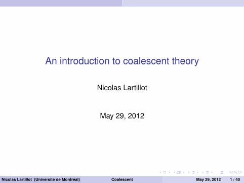
Inferring population history from haplotype data
Hein, Shierup and Wiuf, 2005
a set of n haplotypes randomly sampled from a populationsequences of length L, known mutation rate µwhat can we say about
population size (N) and structure?demographic history?selection?
Nicolas Lartillot (Universite de Montréal) Coalescent May 29, 2012 2 / 40
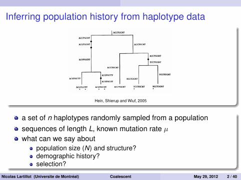
Approachdefine a model of demography and reproduction (Wright-Fisher)induces a law on gene genealogies (Kingman’s coalescent)then define a model of DNA sequence mutationsexplain variation in gene sample based on combination ofmutation and coalescent models.
Applicationsestimating parameters (population size, mutation rate)testing hypotheses (e.g. deviation from neutrality)building blocks for more sophisticated models (course no 2)
Nicolas Lartillot (Universite de Montréal) Coalescent May 29, 2012 3 / 40
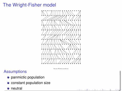
The Wright-Fisher model
Time
from Felsenstein
Assumptionspanmictic populationconstant population sizeneutral
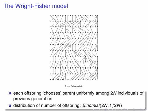
The Wright-Fisher model
Time
from Felsenstein
each offspring ’chooses’ parent uniformly among 2N individuals ofprevious generationdistribution of number of offspring: Binomial(2N,1/2N)
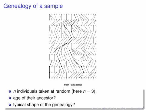
Genealogy of a sample
Time
from Felsenstein
n individuals taken at random (here n = 3)age of their ancestor?typical shape of the genealogy?
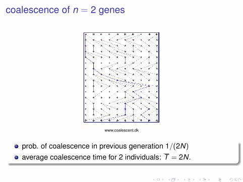
coalescence of n = 2 genes
www.coalescent.dk
prob. of coalescence in previous generation 1/(2N)
average coalescence time for 2 individuals: T = 2N.
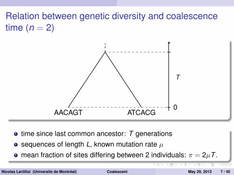
Relation between genetic diversity and coalescencetime (n = 2)
AACAGT ATCACG0
T
time since last common ancestor: T generationssequences of length L, known mutation rate µmean fraction of sites differing between 2 individuals: π = 2µT .
Nicolas Lartillot (Universite de Montréal) Coalescent May 29, 2012 7 / 40
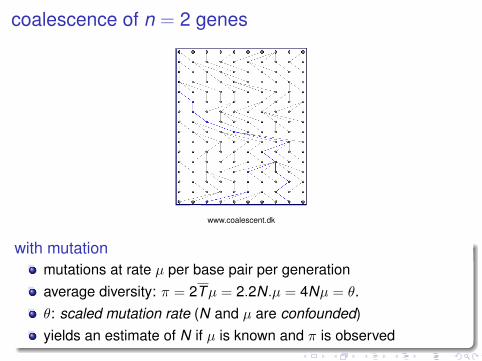
coalescence of n = 2 genes
www.coalescent.dk
with mutationmutations at rate µ per base pair per generationaverage diversity: π = 2Tµ = 2.2N.µ = 4Nµ = θ.θ: scaled mutation rate (N and µ are confounded)yields an estimate of N if µ is known and π is observed
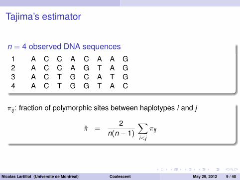
Tajima’s estimator
n = 4 observed DNA sequences1 A C C A C A A G2 A C C A G T A G3 A C T G C A T G4 A C T G G T A C
πij : fraction of polymorphic sites between haplotypes i and j
π̂ =2
n(n − 1)
∑i<j
πij
Nicolas Lartillot (Universite de Montréal) Coalescent May 29, 2012 9 / 40
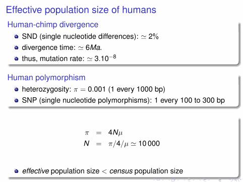
Effective population size of humansHuman-chimp divergence
SND (single nucleotide differences): ' 2%divergence time: ' 6Ma.thus, mutation rate: ' 3.10−8
Human polymorphismheterozygosity: π = 0.001 (1 every 1000 bp)SNP (single nucleotide polymorphisms): 1 every 100 to 300 bp
π = 4NµN = π/4/µ ' 10 000
effective population size < census population size
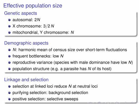
Effective population sizeGenetic aspects
autosomal: 2NX chromosome: 3/2 Nmitochondrial, Y chromosome: N
Demographic aspectsN: harmonic mean of census size over short-term fluctuationsfrequent bottlenecks: low Nreproductive variance (species with male dominance have low N)population structure (e.g. a parasite has N of its host)
Linkage and selectionselection at linked loci reduce N at neutral locipurifying selection: background selectionpositive selection: selective sweeps
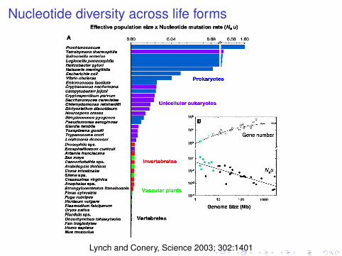
Nucleotide diversity across life forms
Lynch and Conery, Science 2003; 302:1401
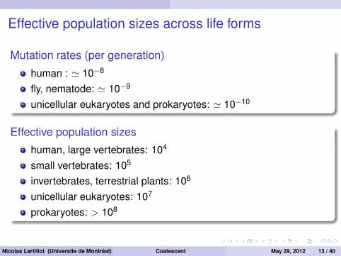
Effective population sizes across life forms
Mutation rates (per generation)
human : ' 10−8
fly, nematode: ' 10−9
unicellular eukaryotes and prokaryotes: ' 10−10
Effective population sizes
human, large vertebrates: 104
small vertebrates: 105
invertebrates, terrestrial plants: 106
unicellular eukaryotes: 107
prokaryotes: > 108
Nicolas Lartillot (Universite de Montréal) Coalescent May 29, 2012 13 / 40
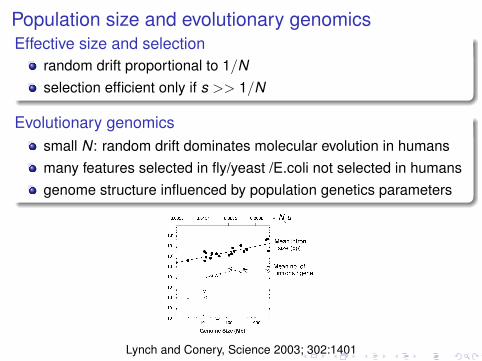
Population size and evolutionary genomicsEffective size and selection
random drift proportional to 1/Nselection efficient only if s >> 1/N
Evolutionary genomicssmall N: random drift dominates molecular evolution in humansmany features selected in fly/yeast /E.coli not selected in humansgenome structure influenced by population genetics parameters
(11). Because degenerative mutations greatlyoutnumber beneficial mutations, the proba-bility of preservation by rare neofunctional-izing mutations is diminished in smallpopulations. In contrast, preservation by sub-functionalization occurs when both membersof a pair are partially degraded by mutationsto the extent that their joint expression isnecessary to fulfill the essential functions ofthe ancestral locus (12, 13). The probabilityof subfunctionalization approaches zero inlarge populations because the long time tofixation magnifies the chances that secondarymutations will completely incapacitate onecopy before joint preservation is completeand because of the weak mutational disad-vantage of harboring two coding regions(14 ). The longer retention time of duplicategenes in small populations is inconsistentwith the predictions for the neofunctionaliza-tion model and opposite to the expected pat-tern if degenerative mutations only lead tocomplete nonfunctionalization of duplicategenes (15), but it is entirely compatible withexpectations under the subfunctionalizationmodel. Thus, although the evolution of mul-ticellularity undoubtedly posed some new se-lective challenges that were met throughneofunctionalization, much of the increase ingene number in multicellular species may nothave been driven by adaptive processes, butrather as a passive response to a geneticenvironment (reduced population size) moreconducive to duplicate-gene preservationby subfunctionalization.
Spliceosomal introns are noncodingstretches of RNA that are excised from thetranscripts of their host protein-coding genes.The mechanisms by which introns originateremain a mystery, but their broad phyloge-netic distribution implies that they and thespliceosome that processes them were presentin the stem eukaryote (16 ). The average num-ber of introns per gene in most multicellularspecies is between four and seven, whereasthe average number for most unicellular eu-
karyotes is less than two. Only two spliceo-somal introns have been found in the kineto-plastid Trypanosoma (17 ), and only a singleone has been found in the diplomonad Giar-dia (18). Understanding this uneven phyloge-netic distribution of introns is a major chal-lenge for evolutionary genomics.
Although natural selection may eventuallyexploit introns for adaptive purposes (16), newlyestablished introns are expected to impose aselective disadvantage (s) on their host genes byincreasing the mutation rate to defective alleles(19). Theory suggests that there is a thresholdvalue of Nes ! 1.0, below which newly arisenintrons can freely drift to fixation and abovewhich intron colonization and maintenance areexceedingly improbable. Qualitatively consistentwith this hypothesis is a threshold genome sizeof "10 Mb, below which introns are very rareand above which they approach an asymptote ofabout seven per gene (Fig. 3). By transformingscales from Fig. 1B, we found that the maximumvalue of Neu that is permissive to intron prolif-eration is "0.015. How does this compare withthe theoretical expectation of Nes ! 1.0?
The minimum selective disadvantage of anallele that contains a new intron is about equal tothe excess-mutation rate to defective allelescaused by alterations at sites involved in splic-ing. The number of base positions (in the intronand surrounding exons) with nucleotide identi-ties that are essential for proper splicing is un-likely to be less than 10 and is plausibly as highas 30 (19). Thus, the net selective disadvantageof an intron-containing allele is at least 10 to 30times as large as u, not including insertion anddeletion mutations, which minimally occur at"10 to 60% of the rate of substitutions per base(20, 21). Because they can alter the spatial con-figuration of key splice-site signatures, the num-ber of insertion and deletion events affectingproper splicing must exceed that for substitu-tions. Thus, the observed threshold value ofNeu ! 0.015 for intron proliferation is reason-ably compatible with the theoretical Nes ! 1.0threshold.
The rather abrupt increase in the averageintron number per gene with increasing ge-nome size is accompanied by a more contin-uous increase in the average intron length(Fig. 3), which has been observed previouslyin more phylogenetically restricted surveys(22, 23). The inverse scaling of the averageintron length with Neu [slope of the logarith-mic regression (#SEM) on Neu $ –0.67 #0.22] is consistent with the hypothesis thatpopulation-size reduction diminishes the ef-ficiency of selection against mildly deleteri-ous insertions into introns. Within genomes,the average intron size increases in regions oflow recombination (24, 25), which may alsobe a consequence of localized reductions ineffective population size resulting from selec-tive sweeps and/or background selection (19,25). An alternative hypothesis that intron sizeacts as a recombination modifier to reduceselective interference among linked sites (24 )is not easily reconciled with the reduction ofintron size and number in compact genomes.
Mobile genetic elements are self-containedgenomic units capable of proliferating withintheir host genomes (26, 27). Hundreds of fam-ilies of these elements exist within eukaryotes,and almost all of them fit into three majorfunctional categories: DNA-based (cut-and-paste) transposons and the long-terminal repeat(LTR) and non-LTR classes of RNA-dependent(copy-and-paste) retrotransposons. The vastmajority of mobile elements are indiscriminatewith respect to insertion sites, and as a conse-quence, their activities often have deleteriouseffects on the host genome. A broad range ofselection coefficients must be associated withinsertions in coding regions, regulatory regions,and intergenic spacers, and because mutationswith negative fitness consequences %%1/(2Ne)are efficiently eliminated by selection, the frac-tion of mobile-element insertions capable ofdrifting to fixation must decline with increasingNe. Because mobile elements gradually acquireinactivating mutations, the long-term survivalof an element family requires the average au-
Fig. 3. The relationship betweenaverage intron size (solid circles)in base pairs (bp) and intronnumber (open circles) and ge-nome size. The regression for in-tron size is highly significant,with an intercept of 1.41# 0.36,a slope of 0.51 # 0.10, and r2 $0.641, df $ 16 (1).
Table 1. Average rates of origin (B) and loss (d ) ofduplicate genes (#SEM). The former is defined asthe probability of a gene duplicating over the timespan required for a silent-site divergence of 1%.The latter is the exponential rate of loss, such thatD $ 1 – e –(0.01d ), or "0.01d for small d, is theprobability of loss by the time silent sites havediverged by 1%, where e is the base of the naturallogarithm (1). The analyses are based on genefamilies containing five or fewer members, andspecies-specific estimates can be found in thesupporting online material (1).
Species B d
Unicellulareukaryotes
0.00405# 0.00130 43.26# 10.15
Metazoanspecies
0.00373# 0.00073 17.80# 2.52
Prokaryotes 0.00238# 0.00038 –
R E P O R T S
www.sciencemag.org SCIENCE VOL 302 21 NOVEMBER 2003 1403
on
Augu
st 3
0, 2
007
ww
w.s
cien
cem
ag.o
rgD
ownl
oade
d fro
m
Lynch and Conery, Science 2003; 302:1401
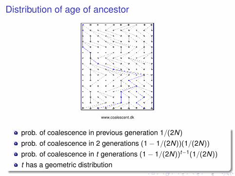
Distribution of age of ancestor
www.coalescent.dk
prob. of coalescence in previous generation 1/(2N)
prob. of coalescence in 2 generations (1− 1/(2N))(1/(2N))
prob. of coalescence in t generations (1− 1/(2N))t−1(1/(2N))
t has a geometric distribution
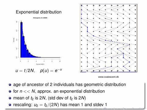
Exponential distributionHistogram of x10000
Exponential(1)
Den
sity
0 2 4 6 8 10
0.0
0.2
0.4
0.6
0.8
u = t/2N, p(u) = e−u
www.coalescent.dk
age of ancestor of 2 individuals has geometric distributionfor n << N, approx. an exponential distributionmean of t2 is 2N, (std dev of t2 is 2N)rescaling: u2 = t2/(2N) has mean 1 and stdev 1
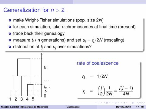
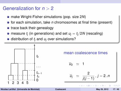
Generalization for n > 2
make Wright-Fisher simulations (pop. size 2N)for each simulation, take n chromosomes at final time (present)trace back their genealogymeasure tj (in generations) and set uj = tj/2N (rescaling)distribution of tj and uj over simulations?
1 2 3 4 50tntn−1
. . .
t2rate of coalescence
r2 = 1/2N
rj =
(j2
)1
2N=
j(j − 1)4N
Nicolas Lartillot (Universite de Montréal) Coalescent May 29, 2012 17 / 40
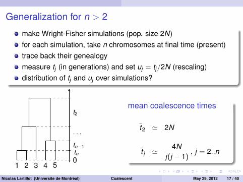
Generalization for n > 2
make Wright-Fisher simulations (pop. size 2N)for each simulation, take n chromosomes at final time (present)trace back their genealogymeasure tj (in generations) and set uj = tj/2N (rescaling)distribution of tj and uj over simulations?
1 2 3 4 50tntn−1
. . .
t2mean coalescence times
t2 ' 2N
t j '4N
j(j − 1), j = 2..n
Nicolas Lartillot (Universite de Montréal) Coalescent May 29, 2012 17 / 40
Generalization for n > 2
make Wright-Fisher simulations (pop. size 2N)for each simulation, take n chromosomes at final time (present)trace back their genealogymeasure tj (in generations) and set uj = tj/2N (rescaling)distribution of tj and uj over simulations?
1 2 3 4 50tntn−1
. . .
t2mean coalescence times
u2 ' 1
uj '2
j(j − 1), j = 2..n
Nicolas Lartillot (Universite de Montréal) Coalescent May 29, 2012 17 / 40
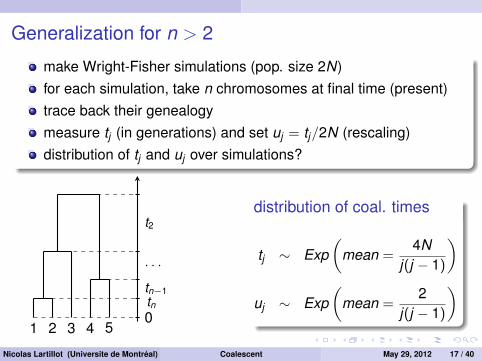
Generalization for n > 2
make Wright-Fisher simulations (pop. size 2N)for each simulation, take n chromosomes at final time (present)trace back their genealogymeasure tj (in generations) and set uj = tj/2N (rescaling)distribution of tj and uj over simulations?
1 2 3 4 50tntn−1
. . .
t2distribution of coal. times
tj ∼ Exp(
mean =4N
j(j − 1)
)
uj ∼ Exp(
mean =2
j(j − 1)
)
Nicolas Lartillot (Universite de Montréal) Coalescent May 29, 2012 17 / 40
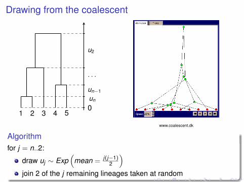
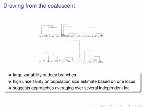
Drawing from the coalescent
1 2 3 4 50un
un−1
. . .
u2
www.coalescent.dk
Algorithmfor j = n..2:
draw uj ∼ Exp(
mean = j(j−1)2
)join 2 of the j remaining lineages taken at random
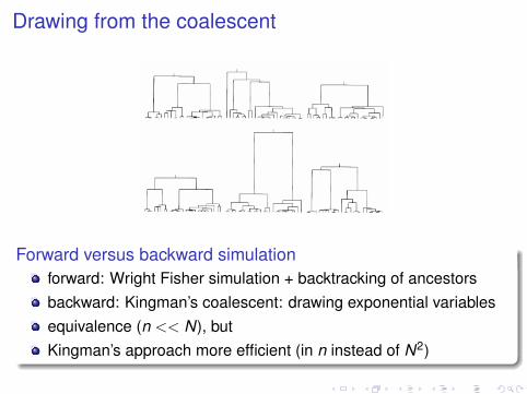
Drawing from the coalescent
Forward versus backward simulationforward: Wright Fisher simulation + backtracking of ancestorsbackward: Kingman’s coalescent: drawing exponential variablesequivalence (n << N), butKingman’s approach more efficient (in n instead of N2)
Drawing from the coalescent
large variability of deep brancheshigh uncertainty on population size estimate based on one locussuggests approaches averaging over several independent loci
What is coalescent theory useful for?
Theoryobtaining insights about patterns in sequence variationderiving theoretical expectations(e.g. age of sample’s last common ancestor)
Simulationsnull distribution for hypothesis testingdetecting departures from neutrality (selection)
Parameter estimationestimating θ = 4Nu based on observed polymorphismestimating demographic scenarios (see course 2)
Nicolas Lartillot (Universite de Montréal) Coalescent May 29, 2012 20 / 40
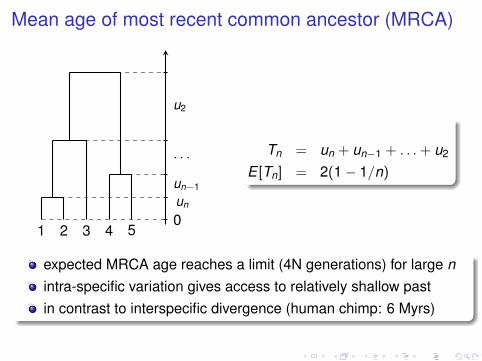
Mean age of most recent common ancestor (MRCA)
1 2 3 4 50un
un−1
. . .
u2
Tn = un + un−1 + . . .+ u2
E [Tn] = 2(1− 1/n)
expected MRCA age reaches a limit (4N generations) for large nintra-specific variation gives access to relatively shallow pastin contrast to interspecific divergence (human chimp: 6 Myrs)
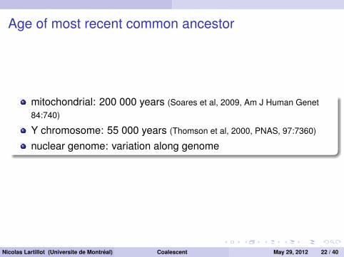
Age of most recent common ancestor
mitochondrial: 200 000 years (Soares et al, 2009, Am J Human Genet84:740)
Y chromosome: 55 000 years (Thomson et al, 2000, PNAS, 97:7360)
nuclear genome: variation along genome
Nicolas Lartillot (Universite de Montréal) Coalescent May 29, 2012 22 / 40
Genealogies and recombination
©!!""6!Nature Publishing Group!
Break point
Coalescence
Time
Present day
Time
TMRCA
Generations
MRCA
DNA fragment
b
c
Induced trees
1
2
4
3
a d
RecombinationPresent daySample
Box 2 | The coalescent
Here we introduce the most popular population genetics model: the coalescent. We begin by introducing the simplest form, in which there is no recombination, and then discuss the version that applies in a more realistic setting.
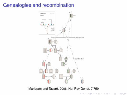
Coalescent without recombination Panels a–c illustrate the intuition that underlies the coalescent using a population of DNA fragments that are evolving according to a Wright–Fisher model — that is, in the absence of recombination, in a population of constant size.
Panel a shows a schematic of an evolving population. In this simplified representation of evolution, each row corresponds to a single generation, and each blue circle denotes a fragment in that generation. Generations are replaced in their entirety by their offspring, with arrows running from the parental fragment to the offspring fragment. The present day is represented by the bottom row, with each higher row representing one generation further back into the past.
Panel b indicates the ancestry of a sample from the present day. In this example, six fragments, indicated in red, are sampled from the current generation. The ancestry of this sample is then traced back in time (that is, up the page), and is indicated in red.
Panel c highlights one of the key features of the coalescent: all information outside the ancestry of the sample of interest can be ignored. The coalescent provides a mathematical description of the ancestry of the sample. As we move back in time, the number of lines of ancestry decreases until, ultimately, a single line remains. The most recent fragment from which the entire sample is descended is known as the ‘most recent common ancestor’ (MRCA), whereas the time at which the MRCA appears is known as the ‘time to the most recent common ancestor’ (TMRCA).
Coalescent with recombinationThe coalescent with recombination is illustrated in panel d. In such settings, lines bifurcate, as well as coalesce (join), as we move back in time. Here we show the genealogy for three copies of a fragment. By tracing the lineages back in time, we observe the following events: in event 1 the green lineage undergoes recombination and splits into two lineages, which are then traced separately; in event 2 one of the resulting green lineages coalesces with the red lineage, creating a segment that is partially ancestral to both green and red, and partially ancestral to red only; in event 3 the blue lineage coalesces with the lineage created by event 2, creating a segment that is partially ancestral to blue and red, and partially ancestral to all three colours; in event 4 the other part of the green lineage coalesces with the lineage created by event 3, creating a segment that is ancestral to all three colours in its entirety. As the inset shows, the recombination event induces different genealogical trees on either side of the break.
Coalescent methods have been reviewed extensively20–22, and there are now book-length treatments97,98 to which the reader is referred for further details.
Panel d is modified with permission from REF. 89 ! (2002) Elsevier.
REVIEWS
762 | OCTOBER 2006 | VOLUME 7 www.nature.com/reviews/genetics
REVIEWS
Marjoram and Tavaré, 2006, Nat Rev Genet, 7:759
Genealogies and recombination
382 | MAY 2002 | VOLUME 3 www.nature.com/reviews/genetics
R E V I EW S
The basic idea underlying the coalescent is that, inthe absence of selection, sampled lineages can be viewedas randomly ‘picking’ their parents, as we go back intime (FIG. 4). Whenever two lineages pick the same par-ent, their lineages coalesce. Eventually, all lineages coa-lesce into a single lineage, the MRCA of the sample. Therate at which lineages coalesce depends on how manylineages are picking their parents (the more lineages, thefaster the rate) and on the size of the population (themore parents to choose from, the slower the rate).
mutation and recombination. We now need a popula-tion-genetics model that incorporates these principlesand that allows us to construct and analyse randomgenealogies. The coalescent has become the standardmodel for this purpose. This choice is not arbitrary, asthe coalescent is a natural extension of classical popu-lation-genetics theory and models7. It was discoveredindependently by several authors in the early1980s12–15, although the definitive treatment is due toKingman12,16.
Tim
e to
MR
CA
Position in kilobases
1.5
2
2.5
3
3.5
0 2 4 6 8 10
a
b c d
e
1 3 2 654
BaAa
1 23 654
b
621543
c
621543
d
621543
e
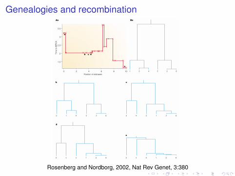
Figure 3 | A simulated sample of six haplotypes using the standard coalescent with recombination. A | In the top graph,the red line shows how the time to the most recent common ancestor (MRCA) (in units of coalescence time — 1 unit correspondsto 2N generations, if N is the size of the population) varies along the chromosome as a result of recombination. The parameters were chosen to represent ~10 kb of human DNA. The crosses along this line mark positions at which recombination took place in the history of the sample. Note that only a fraction of the recombination events resulted in a change of the time to the MRCA. B | A selection of gene trees (a–e) that correspond to specific positions along the chromosome (a–e) is shown. Trees for closelylinked regions tend to be very similar (for example, c and d), if not identical. Numbers 1–6 represent individual haplotypes.
© 2002 Nature Publishing Group
Rosenberg and Nordborg, 2002, Nat Rev Genet, 3:380
Total length of the genealogy
1 2 3 4 50un
un−1
. . .
u2
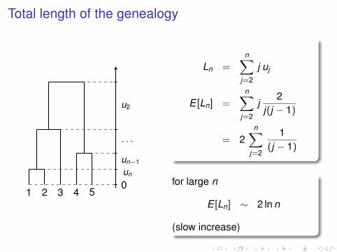
Ln =n∑
j=2
j uj
E [Ln] =n∑
j=2
j2
j(j − 1)
= 2n∑
j=2
1(j − 1)
for large n
E [Ln] ∼ 2 ln n
(slow increase)
Estimating θ = 4Nµ: Watterson’s estimator
1 2 3 4 50un
un−1
. . .
u2
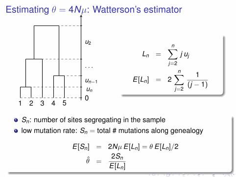
Ln =n∑
j=2
j uj
E [Ln] = 2n∑
j=2
1(j − 1)
Sn: number of sites segregating in the samplelow mutation rate: Sn = total # mutations along genealogy
E [Sn] = 2NµE [Ln] = θE [Ln]/2
θ̂ =2Sn
E [Ln]
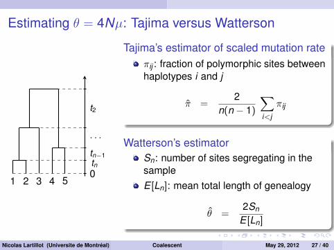
Estimating θ = 4Nµ: Tajima versus Watterson
1 2 3 4 50tntn−1
. . .
t2
Tajima’s estimator of scaled mutation rateπij : fraction of polymorphic sites betweenhaplotypes i and j
π̂ =2
n(n − 1)
∑i<j
πij
Watterson’s estimatorSn: number of sites segregating in thesampleE [Ln]: mean total length of genealogy
θ̂ =2Sn
E [Ln]
Nicolas Lartillot (Universite de Montréal) Coalescent May 29, 2012 27 / 40
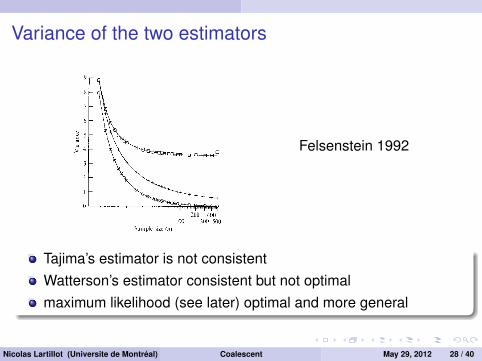
Variance of the two estimators
Felsenstein 1992
Tajima’s estimator is not consistentWatterson’s estimator consistent but not optimalmaximum likelihood (see later) optimal and more general
Nicolas Lartillot (Universite de Montréal) Coalescent May 29, 2012 28 / 40
Demography and population structure
1/14/2010
17
!"#$%&"'(!)*+,(-'"."/*$!0 +-11$)'!-)!
.(2")"!,34,,5,$!4)+$&'%4,6
CHIMPANZÉ TCGCTCTCGTGCCCAGGCTCACCCACAAGTGGTT
HUMAIN1 TTGCTCTCATGCCCAGGCTCACCCACAAGTGGTT
14-1-2010 65
HUMAIN1 TTGCTCTCATGCCCAGGCTCACCCACAAGTGGTT
HUMAIN2 .T......A..................G......
HUMAIN3 .T...G..A.........................
HUMAIN4 .T......A.......A..........G......
!"#$%&'#()!
H1 C G A
H2 C G G
H3 G G A
H4 C A G
Cours BCM6215
7%(&$)'4'"-)!)$'8-%9!:%(&$4*;
14-1-2010 Cours BCM6215 66
<=>?@A
genetree
14-1-2010 Cours BCM6215 67
B-%1$&!.$!C()(4,-C"$&
14-1-2010 68Cours BCM6215
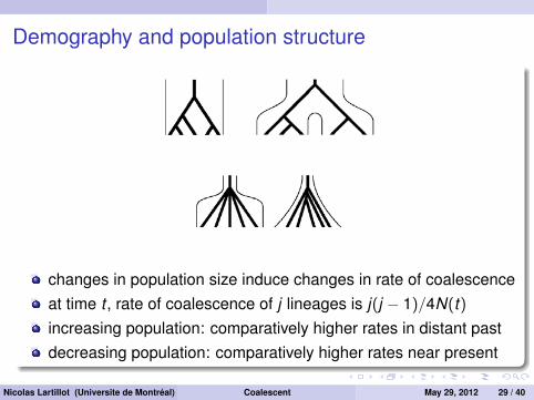
changes in population size induce changes in rate of coalescenceat time t , rate of coalescence of j lineages is j(j − 1)/4N(t)increasing population: comparatively higher rates in distant pastdecreasing population: comparatively higher rates near present
Nicolas Lartillot (Universite de Montréal) Coalescent May 29, 2012 29 / 40
Demography and population structure
1/14/2010
17
!"#$%&"'(!)*+,(-'"."/*$!0 +-11$)'!-)!
.(2")"!,34,,5,$!4)+$&'%4,6
CHIMPANZÉ TCGCTCTCGTGCCCAGGCTCACCCACAAGTGGTT
HUMAIN1 TTGCTCTCATGCCCAGGCTCACCCACAAGTGGTT
14-1-2010 65
HUMAIN1 TTGCTCTCATGCCCAGGCTCACCCACAAGTGGTT
HUMAIN2 .T......A..................G......
HUMAIN3 .T...G..A.........................
HUMAIN4 .T......A.......A..........G......
!"#$%&'#()!
H1 C G A
H2 C G G
H3 G G A
H4 C A G
Cours BCM6215
7%(&$)'4'"-)!)$'8-%9!:%(&$4*;
14-1-2010 Cours BCM6215 66
<=>?@A
genetree
14-1-2010 Cours BCM6215 67
B-%1$&!.$!C()(4,-C"$&
14-1-2010 68Cours BCM6215
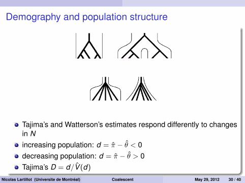
Tajima’s and Watterson’s estimates respond differently to changesin Nincreasing population: d = π̂ − θ̂ < 0decreasing population: d = π̂ − θ̂ > 0Tajima’s D = d/V̂ (d)
Nicolas Lartillot (Universite de Montréal) Coalescent May 29, 2012 30 / 40
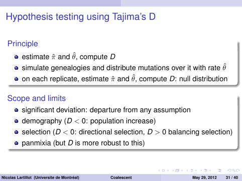
Hypothesis testing using Tajima’s D
Principle
estimate π̂ and θ̂, compute Dsimulate genealogies and distribute mutations over it with rate θ̂on each replicate, estimate π̂ and θ̂, compute D: null distribution
Scope and limitssignificant deviation: departure from any assumptiondemography (D < 0: population increase)selection (D < 0: directional selection, D > 0 balancing selection)panmixia (but D is more robust to this)
Nicolas Lartillot (Universite de Montréal) Coalescent May 29, 2012 31 / 40
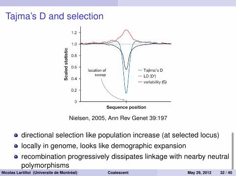
Tajma’s D and selection
ANRV260-GE39-10 ARI 10 October 2005 20:29
Selective sweep:the process by whicha new advantageousmutation eliminatesor reduces variationin linked neutral sitesas it increases infrequency in thepopulation
in explaining the pattern of variability withinand between species (39, 59).
Much of the theoretical literature in pop-ulation genetics over the past 50 years hasfocused on developing and analyzing modelsthat generalize the previously mentioned ba-sic di-allelic models to models where morethan two alleles may be segregating, wheremultiple mutations may arise and interact—possibly in the presence of recombination,where the environment may be changingthrough time, and where random genetic driftmay be acting in populations subject to vari-ous demographic forces (25, 39). From theoryalone we have gained many valuable insights,including the fact that the efficacy of selectiondepends not only on the selection coefficient,but primarily on the product of the selectioncoefficient and the effective population size.An increased effect of selection may be due toeither an increased population size or a largerselection coefficient. Among other important
Figure 1The effect of a selective sweep on genetic variation. The figure is based onaveraging over 100 simulations of a strong selective sweep. It illustrateshow the number of variable sites (variability) is reduced, LD is increased,and the frequency spectrum, as measured by Tajima’s D, is skewed, in theregion around the selective sweep. All statistics are calculated in a slidingwindow along the sequence right after the advantageous allele has reachedfrequency 1 in the population. All statistics are also scaled so that theexpected value under neutrality equals one.
findings is that balancing selection may oc-cur for many reasons other than overdomi-nance, (e.g., fluctuating environmental con-ditions) and could therefore, potentially, bequite common (38, 39). However, the efficacyof selection will tend to be reduced when mul-tiple selected alleles are segregating simulta-neously in the genome. The mutations willtend to interfere with each other and reducethe local effective population size (8, 29, 40,57). Many population geneticists used to be-lieve that the number of selective deaths re-quired to maintain large amounts of selectionwould have to be so large that selection wouldprobably play a very small role in shaping ge-netic variation (43, 60, 61). These types of ar-guments, known as genetic load arguments,were instrumental in the development of theneutral theory. However, the amount of selec-tion that a genome can permit depends on theway mutations interact in their effect on or-ganismal fitness and on several other criticalmodel assumptions (25, 62, 71, 107). Popula-tion genetic theory does not exclude the possi-bility that selection is very pervasive and can-not alone determine the relative importanceand modality of selection in the absence ofdata from real living organisms (25, 39).
Much excitement currently exists in thepopulation genetics communities over the factthat many predictions generated from thetheory may now be tested in the context ofthe large genomic data sets. In particular,we should be able to detect the molecularsignatures of new, strongly selected advanta-geous mutations that have recently becomefixed (reached a frequency of one in the pop-ulation). As these mutations increase in fre-quency, they tend to reduce variation in theneighboring region where neutral variants aresegregating (13, 51, 52, 68). This process, bywhich a selected mutation reduces variabil-ity in linked sites as it goes to fixation, isknown as a selective sweep (Figure 1). Thehope is that by analysis of large compara-tive genomic data sets and large SNP datasets we will be able to determine how andwhere both positive and negative selection
200 Nielsen
Ann
u. R
ev. G
enet
. 200
5.39
:197
-218
. Dow
nloa
ded
from
ww
w.a
nnua
lrevi
ews.o
rgby
Uni
vers
ite d
e M
ontre
al o
n 05
/26/
12. F
or p
erso
nal u
se o
nly.
Nielsen, 2005, Ann Rev Genet 39:197
directional selection like population increase (at selected locus)locally in genome, looks like demographic expansionrecombination progressively dissipates linkage with nearby neutralpolymorphisms
Nicolas Lartillot (Universite de Montréal) Coalescent May 29, 2012 32 / 40
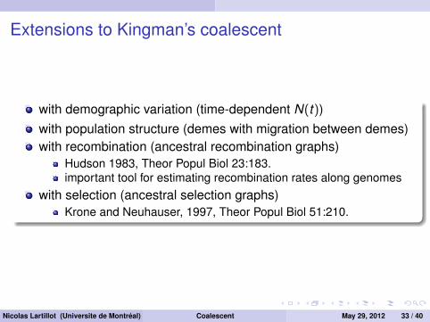
Extensions to Kingman’s coalescent
with demographic variation (time-dependent N(t))with population structure (demes with migration between demes)with recombination (ancestral recombination graphs)
Hudson 1983, Theor Popul Biol 23:183.important tool for estimating recombination rates along genomes
with selection (ancestral selection graphs)Krone and Neuhauser, 1997, Theor Popul Biol 51:210.
Nicolas Lartillot (Universite de Montréal) Coalescent May 29, 2012 33 / 40

Genealogies and recombination
©!!""6!Nature Publishing Group!
Break point
Coalescence
Time
Present day
Time
TMRCA
Generations
MRCA
DNA fragment
b
c
Induced trees
1
2
4
3
a d
RecombinationPresent daySample
Box 2 | The coalescent
Here we introduce the most popular population genetics model: the coalescent. We begin by introducing the simplest form, in which there is no recombination, and then discuss the version that applies in a more realistic setting.
Coalescent without recombination Panels a–c illustrate the intuition that underlies the coalescent using a population of DNA fragments that are evolving according to a Wright–Fisher model — that is, in the absence of recombination, in a population of constant size.
Panel a shows a schematic of an evolving population. In this simplified representation of evolution, each row corresponds to a single generation, and each blue circle denotes a fragment in that generation. Generations are replaced in their entirety by their offspring, with arrows running from the parental fragment to the offspring fragment. The present day is represented by the bottom row, with each higher row representing one generation further back into the past.
Panel b indicates the ancestry of a sample from the present day. In this example, six fragments, indicated in red, are sampled from the current generation. The ancestry of this sample is then traced back in time (that is, up the page), and is indicated in red.
Panel c highlights one of the key features of the coalescent: all information outside the ancestry of the sample of interest can be ignored. The coalescent provides a mathematical description of the ancestry of the sample. As we move back in time, the number of lines of ancestry decreases until, ultimately, a single line remains. The most recent fragment from which the entire sample is descended is known as the ‘most recent common ancestor’ (MRCA), whereas the time at which the MRCA appears is known as the ‘time to the most recent common ancestor’ (TMRCA).
Coalescent with recombinationThe coalescent with recombination is illustrated in panel d. In such settings, lines bifurcate, as well as coalesce (join), as we move back in time. Here we show the genealogy for three copies of a fragment. By tracing the lineages back in time, we observe the following events: in event 1 the green lineage undergoes recombination and splits into two lineages, which are then traced separately; in event 2 one of the resulting green lineages coalesces with the red lineage, creating a segment that is partially ancestral to both green and red, and partially ancestral to red only; in event 3 the blue lineage coalesces with the lineage created by event 2, creating a segment that is partially ancestral to blue and red, and partially ancestral to all three colours; in event 4 the other part of the green lineage coalesces with the lineage created by event 3, creating a segment that is ancestral to all three colours in its entirety. As the inset shows, the recombination event induces different genealogical trees on either side of the break.
Coalescent methods have been reviewed extensively20–22, and there are now book-length treatments97,98 to which the reader is referred for further details.
Panel d is modified with permission from REF. 89 ! (2002) Elsevier.
REVIEWS
762 | OCTOBER 2006 | VOLUME 7 www.nature.com/reviews/genetics
REVIEWS
Marjoram and Tavaré, 2006, Nat Rev Genet, 7:759
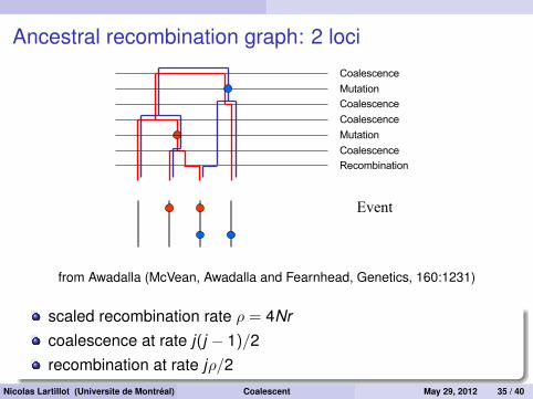
Ancestral recombination graph: 2 loci
4
The ancestral recombination graph
• The combined history of recombination and coalescence is described
by the ancestral recombination graph
Mutation
Mutation
Event
Recombination
Coalescence
Coalescence
Coalescence
Coalescence
Deconstructing the ARG
Learning about recombination
• Just like there is a true genealogy underlying a sample of sequences
without recombination, there is a true ARG underlying samples of
sequences with recombination
• As before, we can consider nonparametric and parametric ways of
learning about recombination
• There are several useful nonparametric ways of learning about
recombination which we will consider first
– These really only apply to species, such as humans, where we can be fairly
surely that most SNPs are the result of a single ancestral mutation event
The signal of recombination?
Recurrent mutation Recombination
Ancestralchromosome
recombines
from Awadalla (McVean, Awadalla and Fearnhead, Genetics, 160:1231)
scaled recombination rate ρ = 4Nrcoalescence at rate j(j − 1)/2recombination at rate jρ/2
Nicolas Lartillot (Universite de Montréal) Coalescent May 29, 2012 35 / 40
Ancestral recombination graph: continuous segmentof loci
JOTU: “chap05” — 2004/10/28 — 13:24 — page 142 — #16
142 5 : The coalescent with recombination
1
3
6
10
6
3
1
!
!
!2
!2
!32
!32
!52
!
!
!
!
Coal. Recomb.
12
Anc. mat.
! + "
12 ! + "
! + "
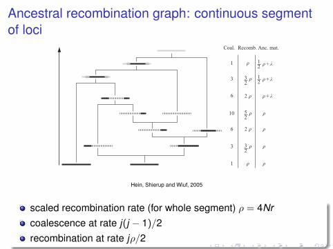
Figure 5.12 Black lines represent the sample sequences or ancestral sequence material tothese. Dotted lines represent non-ancestral material. Light grey lines indicate that a MRCAhas been found. The non-ancestral piece formed after the first coalescence event betweentwo non-consecutive pieces of ancestral material is trapped material. Also shown is the rateof coalescence and recombination, and the amount of material spanned by ancestralmaterial. ! is the length of the black bar in the sequence with dashed ends.
either a coalescent event (with rate k(k ! 1)/2 = 1) or a recombinationevent (with rate k"/2 = ") could occur. In this example the first eventis a recombination event. After the event there are three sequences withancestral material to the two sampled sequences. The next two events arealso recombination events. In one of the two events a sequence is createdwith no material ancestral to the sample. The rate of a coalescence is now10, while the rate of recombination is 2.5".
The fourth event is the first coalescent event that also traps a piece of non-ancestral material between two pieces of ancestral material. As long as theflanking regions are linked, their genealogical histories are identical, so ifone segment coalesces into another sequence, so does the other. After threemore coalescence events all the ancestral material from the two sampledsequences have found common ancestry, in fact have found a GMRCA.There are two MRCAs: one is also the GMRCA which is the MRCA ofthe middle island of ancestral material, the other is the MRCA of the twoflanking islands of ancestral material. This MRCA is created at the secondcoalescent event. When two pieces of ancestral material are bridged togetherthey share fate as long as they are not cut by recombination again. Thematerial between the two pieces is called trapped material.
5.5.1.2 Discrete versus continuous sequencesReal sequences have a discrete number of base pairs rather than an infinitenumber of sites. The infinite sites model described in the previous sectioncan be converted to a discrete model by dividing the continuous interval
Hein, Shierup and Wiuf, 2005
scaled recombination rate (for whole segment) ρ = 4Nrcoalescence at rate j(j − 1)/2recombination at rate jρ/2
Lineage sortingcompatible with the fossil record, if the Millennium man andSahelanthropus are not on the human lineage.
Whole genome sequences of gorilla and orangutan willsoon supplement the already available whole genomesequences of human and chimpanzee [19]. These fourgenomes are so closely related that alignments of large
contiguous parts of the genomes can be constructed. Analysisof such large fragments is challenging because different partsof the alignment will have different evolutionary histories(and thus different genealogies, see Figure 1) because ofrecombination [14,20]. Ideally, one would like to infer thegenealogical changes directly from the data and then analyzeeach type of genealogy separately. A natural approach to thischallenge is to move along the alignment, and simultaneouslycompute the probabilities of different relationships andspeciation times. While recombination has been consideredin previous likelihood models [14], the spatial informationalong the alignment has largely been ignored.In this paper we describe a hidden Markov model (HMM)
that allows the presence of different genealogies along largemultiple alignments. The hidden states are different possiblegenealogies (labeled HC1, HC2, HG, and CG in Figures 1 and2). Parameters of the HMM include population geneticsparameters such as the HC and human–chimp–gorilla (HCG)ancestral effective population sizes, NHC and NHCG, andspeciation times s1 and s2 (see Figure 1). We therefore nameour approach a coalescent HMM (coal-HMM). The statisticalframework of HMMs yields parameter estimates with asso-ciated standard errors, and posterior probabilities of hiddenstates [21–23]. We show by simulation studies that the coal-HMM recovers parameters from the coalescence withrecombination process, and we apply the coal-HMM to fivelong contiguous human–chimp–gorilla–orangutan (HCGO)
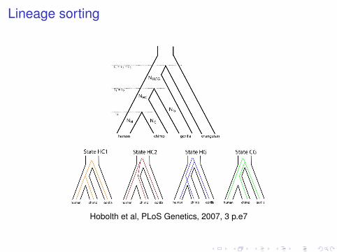
Figure 1. Genetic and Species Relationships May Differ
Top: Genealogical relationship of human, chimpanzee, gorilla, and orangutan. Speciation times are denoted s1, s1! s2, and s1! s2! s3. Population sizesof human, chimpanzee, and gorilla are denoted NH, NC, and NG, while the HC and HCG ancestral population sizes are denoted NHC and NHCG.Bottom: Each of the four hidden states in the coal-HMM corresponds to a particular phylogenetic tree. In state HC1, human and chimpanzee coalescebefore speciation of human, chimpanzee, and gorilla, i.e., before s1 ! s2. In states HC2, HG, and CG, human, chimpanzee, and gorilla coalesce afterspeciation of the three species, i.e., after s1 ! s2. In HC2, the human and chimpanzee lineages coalesce first, and then the HC lineage coalesces withgorilla. In state HG, human and gorilla coalesce first, and in state CG, chimpanzee and gorilla coalesce first. The hidden phylogenetic states cannot beobserved from present-day sequence data, but they can be decoded using the coal-HMM methodology.doi:10.1371/journal.pgen.0030007.g001
PLoS Genetics | www.plosgenetics.org February 2007 | Volume 3 | Issue 2 | e70295
Genomic Relationships of Great Apes
Author Summary
Primate evolution is a central topic in biology and much informationcan be obtained from DNA sequence data. A key parameter is thetime ‘‘when we became human,’’ i.e., the time in the past whendescendents of the human–chimp ancestor split into human andchimpanzee. Other important parameters are the time in the pastwhen descendents of the human–chimp–gorilla ancestor split intodescendents of the human–chimp ancestor and the gorilla ancestor,and population sizes of the human–chimp and human–chimp–gorilla ancestors. To estimate speciation times and ancestralpopulation sizes we have developed a new methodology thatexplicitly utilizes the spatial information in contiguous genomealignments. Furthermore, we have applied this methodology to fourlong autosomal human–chimp–gorilla–orangutan alignments andestimated a very recent speciation time of human and chimp(around 4 million years) and ancestral population sizes much largerthan the present-day human effective population size. We alsoanalyzed X-chromosome sequence data and found that the Xchromosome has experienced a different history from that ofautosomes, possibly because of selection.
Hobolth et al, PLoS Genetics, 2007, 3 p.e7
Lineage sorting: structured coalescentcompatible with the fossil record, if the Millennium man andSahelanthropus are not on the human lineage.
Whole genome sequences of gorilla and orangutan willsoon supplement the already available whole genomesequences of human and chimpanzee [19]. These fourgenomes are so closely related that alignments of large
contiguous parts of the genomes can be constructed. Analysisof such large fragments is challenging because different partsof the alignment will have different evolutionary histories(and thus different genealogies, see Figure 1) because ofrecombination [14,20]. Ideally, one would like to infer thegenealogical changes directly from the data and then analyzeeach type of genealogy separately. A natural approach to thischallenge is to move along the alignment, and simultaneouslycompute the probabilities of different relationships andspeciation times. While recombination has been consideredin previous likelihood models [14], the spatial informationalong the alignment has largely been ignored.In this paper we describe a hidden Markov model (HMM)
that allows the presence of different genealogies along largemultiple alignments. The hidden states are different possiblegenealogies (labeled HC1, HC2, HG, and CG in Figures 1 and2). Parameters of the HMM include population geneticsparameters such as the HC and human–chimp–gorilla (HCG)ancestral effective population sizes, NHC and NHCG, andspeciation times s1 and s2 (see Figure 1). We therefore nameour approach a coalescent HMM (coal-HMM). The statisticalframework of HMMs yields parameter estimates with asso-ciated standard errors, and posterior probabilities of hiddenstates [21–23]. We show by simulation studies that the coal-HMM recovers parameters from the coalescence withrecombination process, and we apply the coal-HMM to fivelong contiguous human–chimp–gorilla–orangutan (HCGO)
Figure 1. Genetic and Species Relationships May Differ
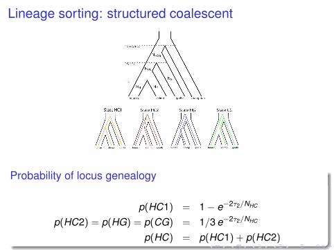
Top: Genealogical relationship of human, chimpanzee, gorilla, and orangutan. Speciation times are denoted s1, s1! s2, and s1! s2! s3. Population sizesof human, chimpanzee, and gorilla are denoted NH, NC, and NG, while the HC and HCG ancestral population sizes are denoted NHC and NHCG.Bottom: Each of the four hidden states in the coal-HMM corresponds to a particular phylogenetic tree. In state HC1, human and chimpanzee coalescebefore speciation of human, chimpanzee, and gorilla, i.e., before s1 ! s2. In states HC2, HG, and CG, human, chimpanzee, and gorilla coalesce afterspeciation of the three species, i.e., after s1 ! s2. In HC2, the human and chimpanzee lineages coalesce first, and then the HC lineage coalesces withgorilla. In state HG, human and gorilla coalesce first, and in state CG, chimpanzee and gorilla coalesce first. The hidden phylogenetic states cannot beobserved from present-day sequence data, but they can be decoded using the coal-HMM methodology.doi:10.1371/journal.pgen.0030007.g001
PLoS Genetics | www.plosgenetics.org February 2007 | Volume 3 | Issue 2 | e70295
Genomic Relationships of Great Apes
Author Summary
Primate evolution is a central topic in biology and much informationcan be obtained from DNA sequence data. A key parameter is thetime ‘‘when we became human,’’ i.e., the time in the past whendescendents of the human–chimp ancestor split into human andchimpanzee. Other important parameters are the time in the pastwhen descendents of the human–chimp–gorilla ancestor split intodescendents of the human–chimp ancestor and the gorilla ancestor,and population sizes of the human–chimp and human–chimp–gorilla ancestors. To estimate speciation times and ancestralpopulation sizes we have developed a new methodology thatexplicitly utilizes the spatial information in contiguous genomealignments. Furthermore, we have applied this methodology to fourlong autosomal human–chimp–gorilla–orangutan alignments andestimated a very recent speciation time of human and chimp(around 4 million years) and ancestral population sizes much largerthan the present-day human effective population size. We alsoanalyzed X-chromosome sequence data and found that the Xchromosome has experienced a different history from that ofautosomes, possibly because of selection.
Probability of locus genealogy
p(HC1) = 1− e−2τ2/NHC
p(HC2) = p(HG) = p(CG) = 1/3 e−2τ2/NHC
p(HC) = p(HC1) + p(HC2)
Estimating ancestral population size
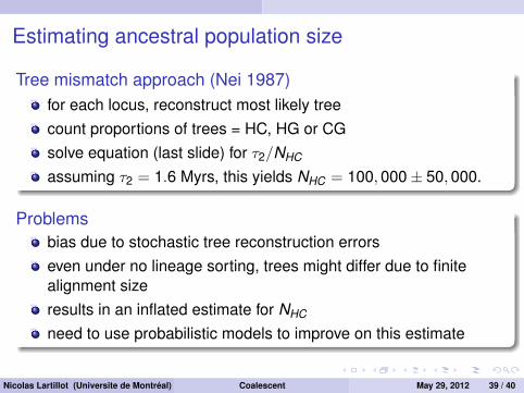
Tree mismatch approach (Nei 1987)for each locus, reconstruct most likely treecount proportions of trees = HC, HG or CGsolve equation (last slide) for τ2/NHC
assuming τ2 = 1.6 Myrs, this yields NHC = 100,000± 50,000.
Problemsbias due to stochastic tree reconstruction errorseven under no lineage sorting, trees might differ due to finitealignment sizeresults in an inflated estimate for NHC
need to use probabilistic models to improve on this estimate
Nicolas Lartillot (Universite de Montréal) Coalescent May 29, 2012 39 / 40
Summary and conclusions
Summaryrate of coalescence of j lineages is j(j − 1)/4Ndepth of genealogy reflects population sizeshape of genealogy reflects demographic historyKingman’s coalescent: simple and powerful model for
understanding population geneticsestimating parameterstesting models
From therecoalescent at the core of probabilistic models for statisticalinferencerepresents the natural law for integrating over unknowngenealogies
Nicolas Lartillot (Universite de Montréal) Coalescent May 29, 2012 40 / 40