Embed Size (px)
Citation preview

Introduction to Coalescent Theory
Mick Elliot & Arne Mooers

What is the coalescent?
The coalescent is a model of the distribution of gene divergence in a genealogy
It is widely used to estimate population genetic parameters such as population size, migration rates and recombination rates in natural populations It was originally formulated as the “n-coalescent” by Kingman (1982). Others refer to it as the “Kingman coalescent” or just the “coalescent” The coalescent model is derived from a simple population genetic model, and the easiest way to understand what it is and how it works is to follow the basic derivation
Kingman 1982

The Wright-Fisher Population Model
Consider a biallelic gene in a diploid organism
As a visual aid, the wing-cases of the ladybirds below are coloured to represent the alleles carried by each individual
Two “red” alleles
Two “yellow” alleles
A “red” and a “yellow” allele

The Wright-Fisher Population Model
Start with a population of size N
Gen
erat
ion
1

The Wright-Fisher Population Model
Gen
erat
ion
1
Start with a population of size N
As soon as an individual dies it is replaced by a new offspring, so the population size remains constant
Gen
erat
ion
2

The Wright-Fisher Population Model
Gen
erat
ion
1 G
ener
atio
n 2
Start with a population of size N
As soon as an individual dies it is replaced by a new offspring, so the population size remains constant
Each individual releases many gametes, and new individuals are drawn randomly from the gamete pool

The Wright-Fisher Population Model
Gen
erat
ion
1 G
ener
atio
n 2
Sewall Wright made an important observation

The Wright-Fisher Population Model
Gen
erat
ion
1 G
ener
atio
n 2
Wright and fisher made an important observation
Probability that an allele in G2 has a parent in G1 = 1

The Wright-Fisher Population Model
Gen
erat
ion
1 G
ener
atio
n 2
Wright and fisher made an important observation
Probability that an allele in G2 has a parent in G1 = 1
Probability that a random allele in G2 has the same parent in G1 = 1/2N

The Wright-Fisher Population Model
Gen
erat
ion
1 G
ener
atio
n 2
Wright and fisher made an important observation
Probability that an allele in G2 has a parent in G1 = 1
Probability that a random allele in G2 has the same parent in G1 = 1/2N
So the probability that two copies of a gene came from the same copy in the previous generation is 1/2N

The Wright-Fisher Population Model
Gen
erat
ion
1 G
ener
atio
n 2
The arrows in this diagram contain a genealogy of genes
We can reveal this genealogy by redrawing the diagram in terms of gene copies rather than individuals (or alleles)

Gen
erat
ion
1 G
ener
atio
n 2
The Wright-Fisher Population Model
1
2

Evolutionary biologists Analyse evolution backwards in time from the present Base their research on a sample of extant individuals rather than knowledge of an entire population Do not know initial population parameters (estimating these parameters may be the purpose of the research) Are concerned with the coalescence of extant genes

The coalescent
It is a model of the distribution of coalescent events on a gene genealogy
Based on a sample of extant gene copies and equipped with our favourite model of evolution, we use the coalescent to estimate population genetic parameters associated with coalescent events
i.e. when was the most recent common ancestor of existing gene copies? What was the population size at the time of the coalescent event? How was the population changing before and after the coalescent event? How frequently do gene copies “go extinct”? What migration regime was operating in the historic population?

The Coalescent
We’re going to stick with the Wright-Fisher model for a while
P(Coalesces 1 generation ago)
1/2N
P(Coalesces 2 generations ago)
(1-1/2N) * 1/2N
P(Coalesces 3 generations ago)
(1-1/2N)2 * 1/2N
P(Coalesces 4 generations ago)
(1-1/2N)3 * 1/2N
P(Coalesced t generations ago)
(1-1/2N)t-1 * 1/2N
Coalescence of two gene copies follows a geometric distribution with mean 2N

The Coalescent
So much for two gene copies. What about k gene copies?
P(coalescence) = k(k-1) * 1 2 2N
Number of pairs of gene copies
Probability that a pair coalesces
There are k(k-1)/2 distinct pairs of genes that could coalesce
The probability that one of these coalesces in the previous generation is given by
Can carry through the math – answer is 4N(1-1/k) (or 2x what it is for a pair)

0
2000
4000
6000
8000
10000
12000
14000
16000
18000
20000
1 2 3 4 5 6 7 8 9 10 11 12 13 14 15 16 17 18 19
Number of alleles
Coal
esce
nce
time
(gen
erat
ions
)
Properties of the Coalescent
N=5000
N=2500
N=1000
We start with 20 alleles and wait for them to coalesce until we reach the most recent common ancestor of all alleles
Half the alleles coalesce in the
first 10% of time
50% of the total coalescence time is spent waiting for the last pair of alleles to coalesce!

Properties of the Coalescent
0
2000
4000
6000
8000
10000
12000
14000
16000
18000
20000
1 2 3 4 5 6 7 8 9 10 11 12 13 14 15 16 17 18 19
Number of alleles
Coal
esce
nce
time
(gen
erat
ions
)
This means that coalescent trees are top-heavy!

Properties of the Coalescent
The fact that most branches coalesce at the top of the tree means that deep tree nodes can be inferred from a small number of gene copies

Properties of the Coalescent
The exponential nature of the time between coalescent events makes the coalescent distribution very noisy. These are tree simulated under a stochastic version of the coalescent with an identical N and k.
http://www.mesquiteproject.org

Properties of the Coalescent
The coalescent can be used to simulate a large number of possible genealogies. Some of these genealogies are more likely than others.
The most likely tree is one in which each coalescence event occurs exactly at the expected time according to the coalescent distribution. The further the topology of the simulated tree is from the expected distribution of the coalescent, the less likely it is to be the REAL history of population coalescence.
High likelihood medium likelihood low likelihood
http://www.mesquiteproject.org

Properties of the Coalescent
What is the coalescence rate per unit time?
We saw earlier that there are k(k-1) possible pairs of alleles that could coalesce
There are 2N alleles in a diploid population
So the average rate of coalescence is k(k-1) / 2N
2
2
= k(k-1)/4N

Summary of the basic coalescent
Expected coalescence time for k alleles is exponentially distributed
with a mean ≈ 4N and coalescence rate of k(k-1)/4N
for diploid populations
with a mean ≈ 2N and coalescence rate of k(k-1)/2N
for haploid populations
with a mean ≈ 2Nf and coalescence rate of k(k-1)/2Nf
for populations of mitochondria
when k is large

The Fisher-Wright model’s assumption of constant N may be inaccurate
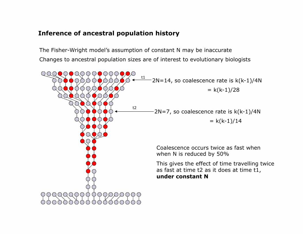
Inference of ancestral population history
http://www.pbs.org
The Fisher-Wright model’s assumption of constant N may be inaccurate
Changes to ancestral population sizes are of interest to evolutionary biologists
Inference of ancestral population history
2N=14, so coalescence rate is k(k-1)/4N
= k(k-1)/28
2N=7, so coalescence rate is k(k-1)/4N
= k(k-1)/14
Coalescence occurs twice as fast when when N is reduced by 50%
This gives the effect of time travelling twice as fast at time t2 as it does at time t1, under constant N
t2
t1

You sample a gene from 10 members of a population
Mick’s basic conceptual understanding of coalescence times and population size...

Mick’s basic conceptual understanding of coalescence time and population size...
You estimate a phylogeny for these 10 members of the population…

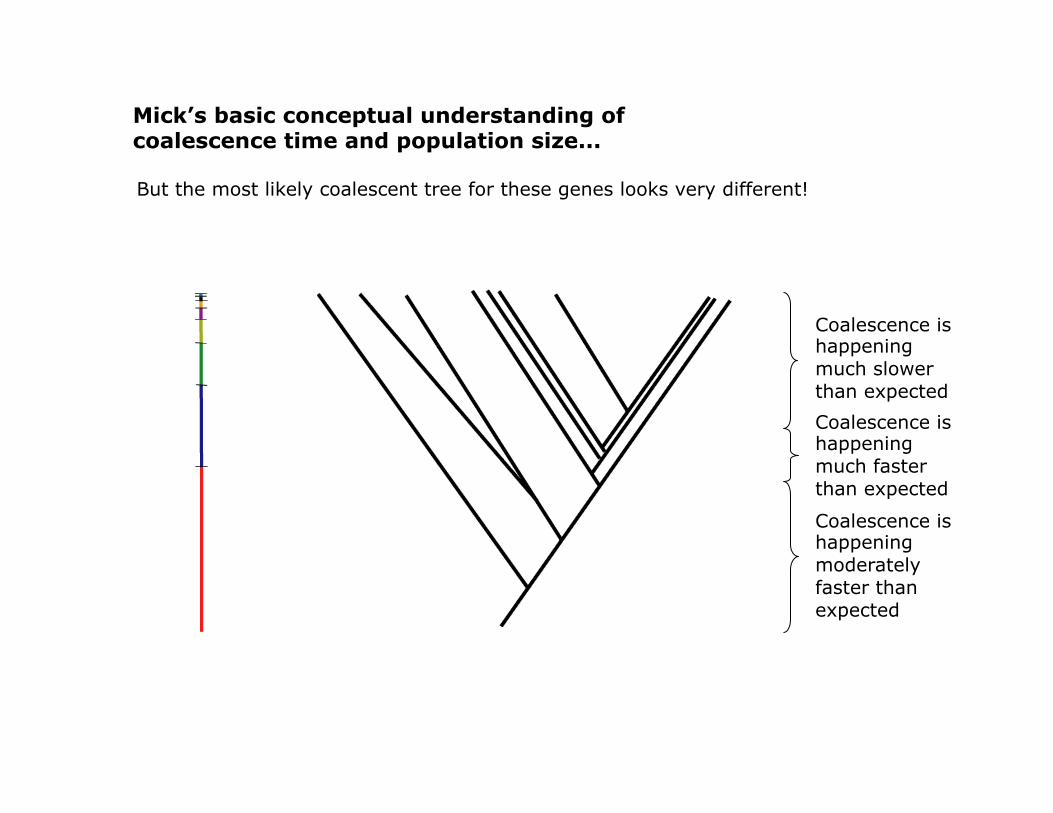
Mick’s basic conceptual understanding of coalescence time and population size...
But the most likely coalescent tree for these genes looks very different!
Mick’s basic conceptual understanding of coalescence time and population size...
But the most likely coalescent tree for these genes looks very different!
Coalescence is happening much slower than expected
Coalescence is happening much faster than expected
Coalescence is happening moderately faster than expected

Mick’s basic conceptual understanding of coalescence time and population size...
But the most likely coalescent tree for these genes looks very different!
Population size is v. large
Population bottleneck!
Medium-large population size

We can use this method for any model of population size change that can be integrated with respect to t
Inference of ancestral population history
time
Population size

Comparative analysis of relative regional population sizes through time.
Atkinson Q D et al. Mol Biol Evol 2007;25:468-474
© The Author 2007. Published by Oxford University Press on behalf of the Society for Molecular Biology and Evolution. All rights reserved. For permissions, please e-mail: [email protected]

Atkinson Q D et al. Mol Biol Evol 2007;25:468-474
Bayesian Skyline Plots of effective population size through time.
mtDNA Variation Predicts Population Size in Humans and Reveals a Major Southern Asian Chapter in Human Prehistory