Embed Size (px)
Citation preview
JSM 2003
AS TIME GOES BY. . .
An Introduction to the Analysis of LongitudinalData
Marie Davidian
Where to get a copy of these slides (and more):
http://www.stat.ncsu.edu/∼davidian
As Time Goes By. . . 1

JSM 2003
Outline
1. Some examples and questions of interest
2. Some ad hoc approaches (and why they might not be so good. . . )
3. How do longitudinal data happen? – A conceptualization
4. Statistical models: Subject-specific and population-averaged
5. Methods for implementation
6. Discussion
As Time Goes By. . . 2

JSM 2003
1. Some examples and questions of interest
Longitudinal studies: Studies where a response is observed on each
participant/unit repeatedly over time are commonplace, e.g.,
• Clinical trials, observational studies in humans, animals
• Studies of growth and decay in agriculture, chemistry
Key messages in this talk:
• The questions of interest may be different, depending on the setting
• Longitudinal data have special features that must be taken into
account to make valid inferences on questions of interest
• Statistical models and methods that acknowledge these features and
the questions of interest are needed
As Time Goes By. . . 3

JSM 2003
First, an “ideal” situation. . .
“World-famous” dental study: Pothoff and Roy (1964)
• 27 children, 16 boys, 11 girls
• On each child, distance (mm) from the center of the pituitary to the
pteryomaxillary fissure measured on each child at ages 8, 10, 12,
and 14 years of age
• A continuous measure of growth
Questions of interest: Informally stated
• Does distance change over time?
• What is the pattern of change?
• Is the pattern different for boys and girls? How?
As Time Goes By. . . 4

JSM 2003
All data (“spaghetti plot ”): 0 = girl, 1 = boy
age (years)
dist
ance
(m
m)
8 9 10 11 12 13 14
2025
30
0 0 0
0
0
0
0
0
0
0
0
1
1
1
1
1
1
1
1
1
1
1
1
1
11
1
0
0
0 0
0
0
0 0
0
0
01
11
1
1
1
11
1
1
11
1
1
1
1 0
0 0 0
0
0
0 0
0
0
0
1
1
1
1
1
1
11
11
11
111
1 0
0 0 0
0
0
0
0
0
0
0
1
1
11
1
1
1
11
1
1
1
1
1
1
1
As Time Goes By. . . 5

JSM 2003
Sample average dental distances: Average across all boys, girls at
each age
8 10 12 14
2122
2324
2526
2728
age
dist
ance
(m
m)
Boys
8 10 12 14
2122
2324
2526
2728
age
dist
ance
(m
m)
Girls
As Time Goes By. . . 6

JSM 2003
Observations:
• All children have all 4 measurements at the same time points (ages)
(“balanced ”)
• Children who “start high ” or “low ” tend to “stay high ” or “low ”
• The individual pattern for most children follows a rough straight line
increase (with some “jitter ”)
• And average distance (across boys and across girls) follows an
approximate straight line pattern
As Time Goes By. . . 7

JSM 2003
Response need not be a continuous measurement. . .
Another “famous” data set: Six Cities Study
• 300 children from six different cities examined annually at ages 9–12
• On each child, respiratory status (1=infection, 0=no infection) and
maternal smoking in past year (1=yes, 0=no)
• Discrete (binary) response
Questions of interest: Informally stated
• Is there an association between child’s respiratory status and
mother’s smoking behavior?
• Does the association change with age ?
Observations:
• Graphical depiction not really informative (binary response)
• Further complication: Missing data at some ages for some
mother-child pairs
As Time Goes By. . . 8

JSM 2003
Pharmacokinetics of theophylline:
• 12 subjects each given oral dose at time 0
• Blood samples at 10 time points over next 25 hours, assayed for
theophylline concentration
Questions of interest: Informally stated
• Understand processes of absorption, elimination, distribution in the
population of subjects like these
⇒ Dosing recommendations
• What is the “typical ” behavior of these processes?
• To what extent does it differ across subjects?
As Time Goes By. . . 9

JSM 2003
Data for 12 subjects: Concentration vs. time
Time (hr)
The
ophy
lline
Con
c. (
mg/
L)
0 5 10 15 20 25
02
46
810
12
As Time Goes By. . . 10

JSM 2003
Standard practice: A “theoretical model ” for each subject
• Represent the body of ith subject by a mathematical compartment
model following oral dose D
Concentration at time t:
Ci(t) =kaiD
Vi(kai − kei){exp(−keit)− exp(−kait)}
• Fractional absorption rate kai, fractional elimination rate kei,
volume of distribution Vi characterize absorption, elimination,
distribution processes for subject i
As Time Goes By. . . 11

JSM 2003
Observations:
• Not balanced (different times for different subjects)
• Concentration-time patterns same shape, but differ for different
subjects
• Theory: This is because kai, kei, Vi differ across subjects
⇒ Learn about “typical ” (average) values and extent of variation of
kai, kei, Vi in population of subjects
Note: The question of interest needs to refer to the pharmacokinetic
one-compartment model
As Time Goes By. . . 12

JSM 2003
Summary: Different questions in different settings
• Characterize and compare patterns of change over time
• Assess associations that evolve over time
• Learn about features underlying observed patterns
Summary: Features of data
• Different types of response (continuous, discrete)
• Subjects observed only intermittently. . .
• . . . at possibly different time points with responses we intended to
collect missing for some subjects (so at the very least not balanced)
As Time Goes By. . . 13

JSM 2003
2. Some ad hoc approaches
Dental study: 16 boys, 11 girls, distance measured at 8, 10, 12, 14
years of age, no missing observations
• Focus: Is dental distance over time (pattern) different for boys and
girls?
Favorite ad hoc analysis:
• Cross-sectional analysis comparing means (boys vs. girls) at each
age 8, 10, 12, 14 (two-sample t-tests)
• P-values: 0.08, 0.06, 0.01, 0.001
• Conclusion ? Multiple comparisons ?
• How to “put this together ” to say something about the differences
in patterns and how they differ? What are the patterns, anyway?
As Time Goes By. . . 14

JSM 2003
Problem: We’re trying to force a familiar analysis to address questions
it’s not designed to answer!
• In fact, what if the data weren’t balanced?
• Need to start with a formal model for the situation that
acknowledges the data structure. . .
Better: (Univariate) repeated measures analysis of variance model
• For subject i in group ` at the jth time
yi`j = µ+τ`+γj+(τγ)`j+bi`+ei`j , bi`iid∼ N (0, σ2
b ), ei`jiid∼ N (0, σ2
e)
Population mean for group `, time j = µ + τ` + γj + (τγ)`j
• Is pattern different for girls and boys?
⇒ (τγ)`j = 0 for all `, j ⇔ mean profiles are parallel across groups
As Time Goes By. . . 15

JSM 2003
Drawbacks:
• Requires data to be balanced
• May be too simple to capture key features of longitudinal data
• Doesn’t explicitly acknowledge time or exploit apparent smooth,
meaningful patterns
• What if the data are discrete ?
For the dental data: Individual child and gender-averaged trajectories
look like straight lines. . .
As Time Goes By. . . 16

JSM 2003
Gender-averaged trajectories: Means across boys, girls at each time
8 10 12 14
2122
2324
2526
2728
age
dist
ance
(m
m)
Boys
8 10 12 14
2122
2324
2526
2728
age
dist
ance
(m
m)
Girls
Impression: Population mean distances lie approximately on a straight
line over time for each gender
As Time Goes By. . . 17

JSM 2003
Question of interest, more formally: Assuming that population means
follow a straight line pattern over time for each gender
• Is pattern different for girls and boys?
⇒ Are the slopes of the population mean profiles different for boys
and girls?
Perspective: These are questions about how the population means are
related over time
Suggests: Ad hoc analysis based on regression model for populations of
girls and boys
• For subject i at age tij ,
yij = β0G+β1Gtij+eij if i is girl, yij = β0B+β1Btij+eij if i is boy,
• Fit by usual OLS, test if β1G = β1B
• But are yij (eij) all uncorrelated (required for OLS)?
As Time Goes By. . . 18

JSM 2003
Individual trajectories: Girls
8 9 10 11 12 13 14
2025
30
age (years)
dist
ance
(m
m)
8 9 10 11 12 13 14
2025
30
age (years)
dist
ance
(m
m)
Impression: Each girl’s distance measurements follow an approximate
straight line trajectory with possibly different slopes across girls (similarly
for boys)
As Time Goes By. . . 19

JSM 2003
Question of interest, more formally: Assuming that each child has
his/her own underlying straight-line trajectory
• Is pattern different for girls and boys?
⇒ Is the “typical ” (average) slope among girls different from that
for boys?
Perspective: These are questions about individual profiles over time
Suggests: Ad hoc analysis based on individual regression models
• For subject i at age tij , yij = β0i + β1itij + eij , E(eij) = 0
• Fit to each child by OLS and do two-sample t-test using estimated
individual slopes
• But are yij all uncorrelated? What if data aren’t balanced?
As Time Goes By. . . 20
JSM 2003
Need a more formal approach. . .
As Time Goes By. . . 21

JSM 2003
3. How do longitudinal data happen?
Idea: Conceptualize how longitudinal data come about and use as a
basis for developing formal statistical models that lead to appropriate
methods for analysis. . .
As Time Goes By. . . 22

JSM 2003
Three hypothetical subjects: (a) What we see, and (b) a
conceptualization of what’s underlying it
time
resp
onse
(a)
time
resp
onse
(b)
As Time Goes By. . . 23

JSM 2003
Features of the conceptual model:
• Each subject has an “inherent trend ” or “trajectory ”
• Actual values might “fluctuate ” about the trend
• Errors in measurement in ascertaining values might occur
(continuous response)
• Averaging over all possible values/measurements for all possible
subjects in the population at each time yields the bold population
mean profile
Remarks:
• Individual trajectories and population mean profile need not be
straight lines (think of theophylline)
• Can think similarly for discrete data (Six Cities)
As Time Goes By. . . 24

JSM 2003
A key feature: Correlation
• Reasonable to suppose that measurements on different subjects are
unrelated ⇒ independent, however. . .
• Measurements on the same subject tend to be “high ” or “low ”
together, so that measurements on the same subject are “more
alike ” than measurements from different subjects
⇒ Measurements on the same subject are correlated due to
among-individual variation
• Values close together in time might tend to “fluctuate ” similarly, so
that measurements on a given subject are “more alike ” the closer
together they are in time
⇒ Measurements on the same subject are correlated due to
within-individual covariation
As Time Goes By. . . 25

JSM 2003
Result: A statistical model must acknowledge that
• While observations on different subjects may be reasonably thought
of as independent. . .
• . . . Observations on the same subject are correlated due to at least
one of these phenomena
Critical point: If we ignore correlation, we act as though we have more
information than we actually do, and analyses will be flawed
• Can be shown formally by statistical theory
• Statistical models and methods must this acknowledge correlation !
As Time Goes By. . . 26

JSM 2003
4. Statistical models for longitudinal data
Two popular types: Corresponding to the two perspectives on the
dental data
• Subject-specific models
• Population-averaged (aka marginal) models
• Depending on the questions in a particular situation, one may be
more suitable then the other
Here: In terms of dental data (continuous response, straight-line
population mean and individual patterns) and then generalize
As Time Goes By. . . 27
JSM 2003
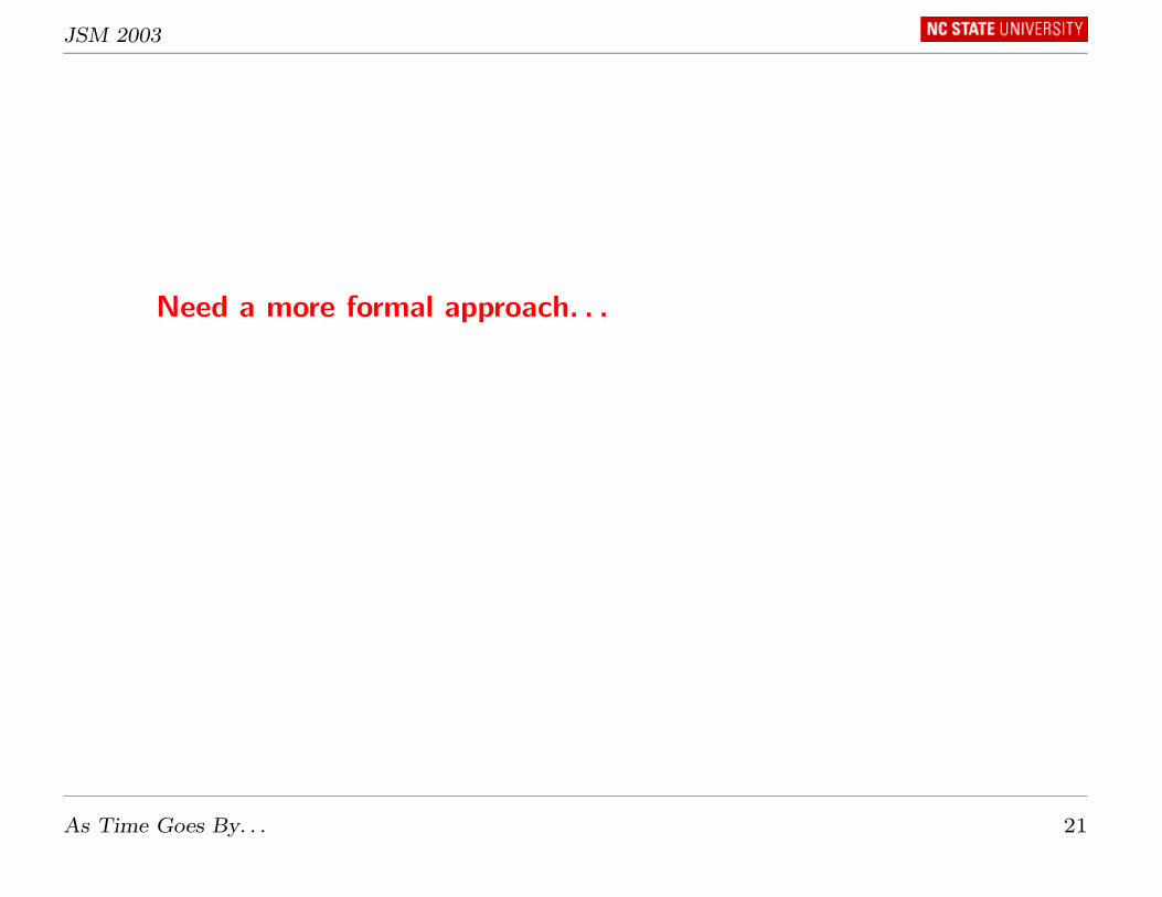
Subject-specific model:
• Model individual behavior
• Questions of interest are about “typical ” (average) such behavior
Dental data: For randomly chosen subject i, measure yij at several
times tij (need not be the same for all i)
yij = β0i + β1itij + ef,ij + eme,ij︸ ︷︷ ︸eij
• β0i, β1i are individual-specific intercept, slope dictating i’s “inherent
trajectory ” β0i + β1itij
• ef,ij is mean-zero deviation from inherent trajectory due to
“fluctuation ” at tij
• eme,ij is mean-zero deviation from inherent trajectory due to error in
measurement at tij
As Time Goes By. . . 28

JSM 2003
Conceptualization: yij = β0i + β1itij + ef,ij + eme,ij︸ ︷︷ ︸eij
time
resp
onse
(a)
time
resp
onse
(b)
As Time Goes By. . . 29
JSM 2003
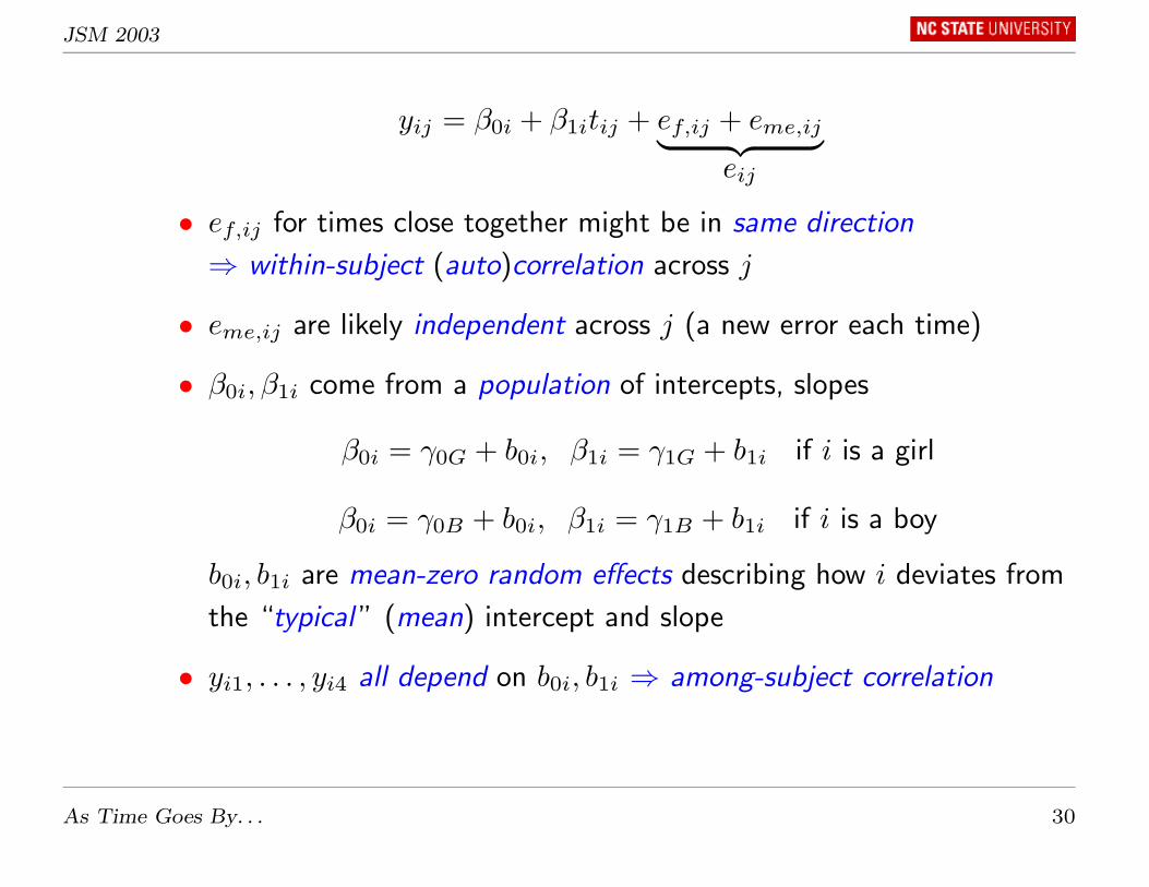
yij = β0i + β1itij + ef,ij + eme,ij︸ ︷︷ ︸eij
• ef,ij for times close together might be in same direction
⇒ within-subject (auto)correlation across j
• eme,ij are likely independent across j (a new error each time)
• β0i, β1i come from a population of intercepts, slopes
β0i = γ0G + b0i, β1i = γ1G + b1i if i is a girl
β0i = γ0B + b0i, β1i = γ1B + b1i if i is a boy
b0i, b1i are mean-zero random effects describing how i deviates from
the “typical ” (mean) intercept and slope
• yi1, . . . , yi4 all depend on b0i, b1i ⇒ among-subject correlation
As Time Goes By. . . 30

JSM 2003
yij = β0i + β1itij + ef,ij + eme,ij︸ ︷︷ ︸eij
,β0i = γ0G or B + b0i
β1i = γ1G or B + b1i
Technically speaking:
• Within-subject autocorrelation: (ef,i1, . . . , ef,i4)T is multivariate
normal with covariance matrix σ2fHi
• Measurement error: (eme,i1, . . . , eme,i4)T is multivariate normal
with diagonal covariance matrix σ2eIi
• “Steep/shallow” slopes associated with “high/low” intercepts
⇒ (b0i, b1i)T correlated with covariance matrix D (assumed
multivariate normal)
Combining: yij = γ0G or B + γ1G or Btij + b0i + b1itij + eij
Can summarize in matrix form. . . yi = (yi1, . . . , yi4)T
As Time Goes By. . . 31

JSM 2003
Linear mixed effects model:
yi = Xiγ + Zibi + ei
γ =
γ0G
γ1G
γ0B
γ1B
, bi =
b0i
b1i
, Zi =
1 ti1...
...
1 ti4
Xi =
1 ti1 0 0...
......
...
1 ti4 0 0
for i a girl , Xi =
0 0 1 ti1...
......
...
0 0 1 ti4
for i a boy
E(yi) = Xiγ, var(yi) = ZiDZTi + σ2
fHi + σ2eIi = Vi
so that
yi ∼MVN (Xiγ, Vi)
As Time Goes By. . . 32
JSM 2003
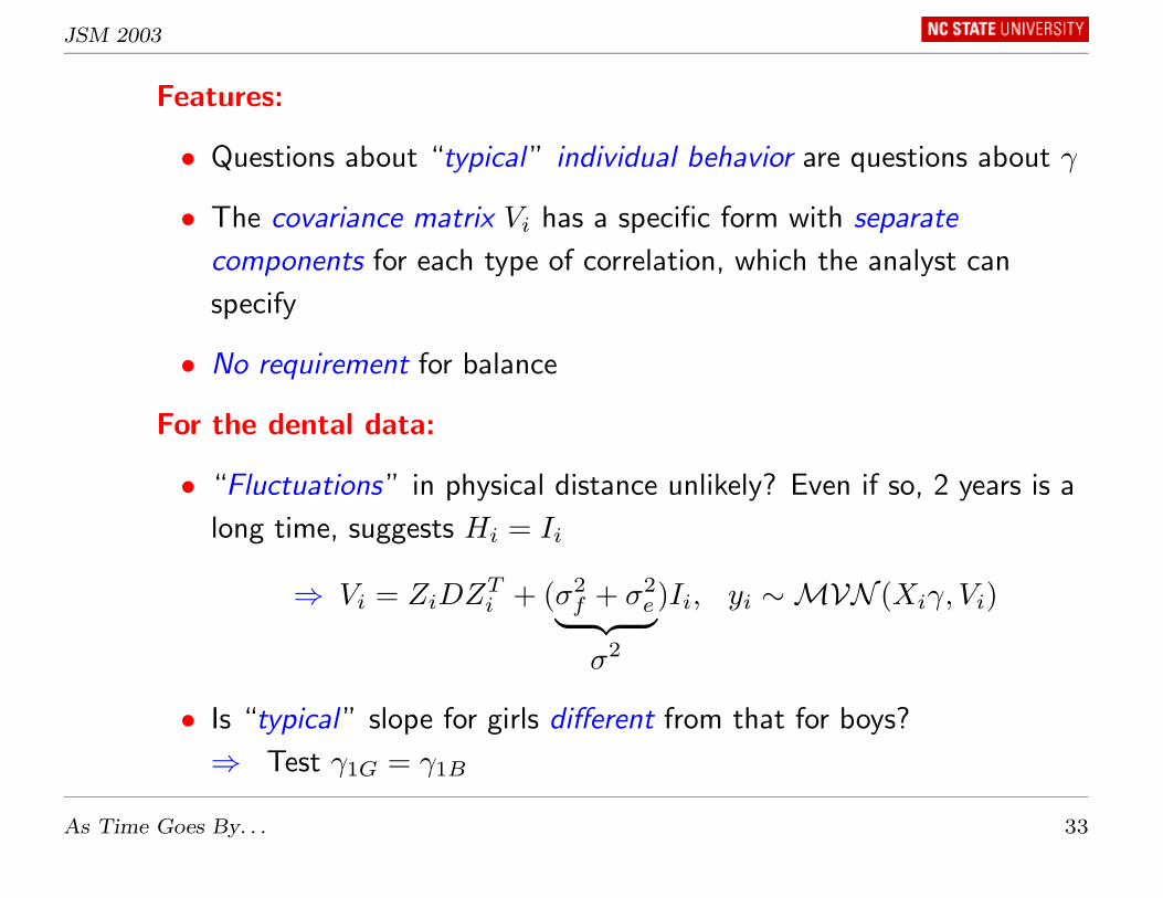
Features:
• Questions about “typical ” individual behavior are questions about γ
• The covariance matrix Vi has a specific form with separate
components for each type of correlation, which the analyst can
specify
• No requirement for balance
For the dental data:
• “Fluctuations ” in physical distance unlikely? Even if so, 2 years is a
long time, suggests Hi = Ii
⇒ Vi = ZiDZTi + (σ2
f + σ2e︸ ︷︷ ︸
σ2
)Ii, yi ∼MVN (Xiγ, Vi)
• Is “typical ” slope for girls different from that for boys?
⇒ Test γ1G = γ1B
As Time Goes By. . . 33

JSM 2003
Population-averaged model:
• Model population behavior by directly modeling the population
mean profile; i.e., E(yi)
• Questions are about how population means are related over time
• Instead of worrying about separate components of var(yi) (within-
and among-individual sources of correlation), just model their
combined effect directly
As Time Goes By. . . 34

JSM 2003
Conceptualization:
time
resp
onse
(a)
time
resp
onse
(b)
As Time Goes By. . . 35

JSM 2003
Dental data: For randomly chosen subject i measure yij at several
times tij (need not be the same for all i)
yij = β0G + β1Gtij + εij for girls, yij = β0B + β1Btij + εij for boys
• E.g., β0G + β1Gtij is the bold population mean profile for girls
• εij is a deviation from the population mean due to the sum total of
among-subject variation, and within-subject fluctuation and
measurement error at tij
Thus, εij are correlated ⇒ specify a covariance matrix
• Question of whether the patterns are different for boys and girls:
Are the slopes of the population mean profiles the same?
⇒ Test β1G = β1B
As Time Goes By. . . 36

JSM 2003
Population-averaged model: In matrix form
yi = Xiβ + εi, β =
β0G
β1G
β0B
β1B
Xi =
1 ti1 0 0...
......
...
1 ti4 0 0
for i a girl , Xi =
0 0 1 ti1...
......
...
0 0 1 ti4
for i a boy
• Implies E(yi) = Xiβ (average over all individuals, fluctuations,
errors)
• Choose a “working model ” for the covariance matrix var(εi) = Σi
that (hopefully) captures the overall combined correlation
• Thus, model is E(yi) = Xiβ, var(yi) = Σi (can add normality)
As Time Goes By. . . 37

JSM 2003
Contrasting the models:
Subject-specific: yi = Xiγ + Zibi + ei, and averaging these individual
models over all bi and ei (so over all subjects, fluctuations, and
measurement errors) gives E(yi) = Xiγ
Population-averaged: yi = Xiβ + εi, and we model this average
directly as E(yi) = Xiβ
Result: The models for the population means at all time points are of
the same form with either model!
• Thus γ and β describe the same thing (population mean profile), so
are really the same . . .
• . . . and we can interpret them either way, e.g., “typical slope ” or
slope of the population average profile !
• The distinction between subject-specific and population-averaged
ends up not mattering, so choose the interpretation you like best!
As Time Goes By. . . 38

JSM 2003
Warning: This changes when the model is nonlinear. . .
As Time Goes By. . . 39

JSM 2003
What about discrete data? Six Cities data
Subject-specific model: Model individual propensity for respiratory
infection (yij = 1) when exposed to maternal smoking xij (=0 or 1)
log(
P (yij = 1|bi)1− P (yij = 1|bi)
)= β0i + β1ixij , β0i = γ0 + b0i, β1i = γ1 + b1i
P (yij = 1|bi) is the probability of infection for child i in particular
• β0i is the log odds of respiratory infection for child i when mother
does not smoke
⇒ γ0 is the “typical ” (mean) value of the log odds for children in
the population
• β1i is the log odds ratio for respiratory infection when child i is
exposed to smoking relative to not, and γ1 is the “typical ” value of
the log odds ratio
⇒ Thus, γ1 = 0 asks whether the “typical ” odds ratio for children
in the population is equal to 1
As Time Goes By. . . 40

JSM 2003
Population-averaged model: Model “average propensity ” for
respiratory infection in the population directly
log(
P (yij = 1)1− P (yij = 1)
)= β0 + β1xij
P (yij = 1) is the probability a child in the population under maternal
smoking xij will have a respiratory infection
• β0 is the log odds of respiratory infection in the population of
children whose mothers don’t smoke
• β1 is the log odds ratio for respiratory infection if the population
were exposed to smoking relative to not
• Thus, β0 and β1 describe what happens “on average” in the
population (as opposed to for a particular individual child)
• . . . and β1 = 0 asks whether the odds ratio for the population is
equal to 1
As Time Goes By. . . 41

JSM 2003
Contrasting the models:
Population-averaged: P (yij = 1) =exp(β0 + β1xij)
1 + exp(β0 + β1xij)
• A model for the average over all children in the population
Subject-specific: P (yij = 1|bi) =exp(γ0 + γ1xij + b0i + b1ixij)
1 + exp(γ0 + γ1xij + b0i + b1ixij)
• A model specifically for the ith child
• The average of this over all children (so over all b0i, b1i) is a very
complicated mess, that does not have the same form as the
population-averaged model above!
Result: In contrast to linear models, for nonlinear models like this, β
and γ have distinct interpretations
As Time Goes By. . . 42

JSM 2003
Back to the examples: Which perspective/model makes more sense?
• Dental data: linear model, can go either way! (Either interpretation
valid!)
• Six Cities data: For inferences to be used for public policy
recommendations, what happens on average in the population is
usually more relevant then what happens to individuals
⇒ population-averaged model
• Theophylline PK data: Interest clearly focused on “typical values ”
and variation of kai, kei, Vi ⇒ subject-specific model
yij =kaiD
Vi(kai − kei){e−keit − e−kait}+ eij
kai = γ1 + bka,i, kei = γ2 + bke,i, Vi = γ3 + bV,ie
⇒ Subject-specific model
Nonlinear mixed effects model
Message: Choose the model that best addresses the questions!
As Time Goes By. . . 43

JSM 2003
5. Methods for implementation
Linear models: Covariance matrix plays key role!
Population-averaged models: Solve generalized estimating equations
(GEE) for β and parameters in var(yi) = Σi
n∑i=1
XTi Σ̂−1
i (yi−Xiβ̂) = 0 which yields β̂ =
(n∑
i=1
XTi Σ̂−1
i Xi
)−1 n∑i=1
XT Σ̂−1i yi
• SAS proc genmod
Subject-specific models: Likelihood methods based on
yi ∼MVN (Xiγ, Vi) to estimate γ and parameters in Vi lead to the
same approach !
γ̂ =
(n∑
i=1
XTi V̂ −1
i Xi
)−1 n∑i=1
XT V̂ −1i yi
• SAS proc mixed, Splus/R lme( )
As Time Goes By. . . 44

JSM 2003
Nonlinear models: Covariance matrix still plays key role, but SS and
PA no longer the same
Population-averaged models: Solve similar generalized estimating
equations (GEEs) for β and parameters in var(yi) = Σi
• SAS proc genmod
Subject-specific models: Much messier! (Likelihood methods)
• E.g., for binary data, must find the average of
P (yij = 1|bi) =exp(γ0 + γ1xij + b0i + b1ixij)
1 + exp(γ0 + γ1xij + b0i + b1ixij)
over b0i, b1i, an integral
• Generalized linear mixed or nonlinear mixed effects model
• SAS proc nlmixed, %glimmix, %nlinmix, Splus/R nlme( )
As Time Goes By. . . 45

JSM 2003
6. Discussion
Main message: Specialized statistical models are required for
longitudinal data analysis – choose the one that’s right for you!
Benefit: Understanding the basis for the models and the role of
correlation is essential to understanding how to use the software!
As Time Goes By. . . 46

JSM 2003
What we didn’t talk about: Lots!
• More advanced modeling considerations
• How to choose appropriate covariance models and what happens if
we’re wrong
• How to select the best model and diagnose how well a model fits
• Details of implementation
• What happens if assumptions are incorrect
• How to handle missing data and dropout
• Other types of models (e.g., transition models)
As Time Goes By. . . 47

JSM 2003
Where to learn more: Some references
• Diggle, P.J., Heagerty, P., Liang, K.-Y., and Zeger, S.L. (2002)
Analysis of Longitudinal Data, 2nd Edition, Oxford University
Press.
• Verbeke, G. and Molenberghs, G. (2000) Linear Mixed Models forLongitudinal Data, Springer.
• Davidian, M. and Giltinan, D.M. (1995) Nonlinear Models forRepeated Measurement Data, Chapman and Hall/CRC Press.
Where to get a copy of these slides (and more):
http://www.stat.ncsu.edu/∼davidian
As Time Goes By. . . 48