Embed Size (px)
Citation preview

1
An Introduction to the Latent Class Model
28 – 29 April 2011
University of Texas – Dallas
A. L. McCutcheon, Ph.D.
Donald O. Clifton Chair of Survey ScienceDirector, Gallup Research Center
Chair, Graduate program in Survey Research and MethodologyProfessor, Statistics and Sociology
University of Nebraska-Lincoln
Email: [email protected]
Introduction to the Latent Class Model 2
www.unl.edu/ALM

2
Software
Glimmix (Michel Wedel)[email protected]
Latent Gold (Jeroen Vermunt)Latent Gold (Jeroen Vermunt)[email protected]
Mplus (Bengt &Linda Muthén)support @statmodel.com
LEM (Jeroen Vermunt)
Introduction to the Latent Class Model 3
Panmark (F. van de Pol)[email protected]
Levels of Measurement
• Continuous (metric quantitative)• Continuous (metric, quantitative)– Ratio
• True zero
• Known metric
• Ordered
• Mutually exclusive categories
Interval
Introduction to the Latent Class Model 4
– Interval• Known metric
• Ordered
• Mutually exclusive categories

3
Levels of Measurement (cont.)
• Categorical (discrete qualitative)• Categorical (discrete, qualitative)– Ordinal
• Ordered
• Mutually exclusive categories
– NominalM ll l i i
Introduction to the Latent Class Model 5
• Mutually exclusive categories
• Latent class analysis focuses primarily on categorical data
Variable Types
• Observability• Observability– Manifest variables
• Directly observed (e.g., frequency of church attendance)
• Indicator variables
Latent variables
Introduction to the Latent Class Model 6
– Latent variables• Indirectly observed (e.g., religiosity)
• Frequently, variables of true interest

4
Variable Types (cont.)
• Causality• Causality– Independent (effects) variables
– Dependent (response) variables
– Intervening (mediating) variables
• Basic LCA’s are non-causal in the
Introduction to the Latent Class Model 7
traditional meaning of the term
Motivating Example
1. You are riding in a car driven by a close friend, and he hits a pedestrian. You know that he is going at least 35 miles an ho r in a 20 mile an ho r speed one There are no otheris going at least 35 miles an hour in a 20-mile-an-hour speed zone. There are no other witnesses. His lawyer says that if you testify under oath that the speed was only 20 miles an hour, it may save him from serious consequences. What right has your friend to expect you to protect him? (Universalistic: He has no right as a friend to expect me to testify to the lower figure.)
2. As a drama critic, your friend asks you to “go easy on a review” of a bad play in which all of his saving are invested.
3. As a physician, your friend asks you to “shade doubts” about a physical examination for an
Introduction to the Latent Class Model 8
3. As a physician, your friend asks you to shade doubts about a physical examination for an insurance policy.
4. As a member of the board of directors, does your friend have a right to expect that you “tip him off” about financially ruinous, though secret, company information.

5
Motivating Example
Samuel A. Stouffer and Jackson Toby (1951) “Role Conflict and Personality,” American Journal of Sociology 56: 395-406.
1 2 3 4 1 2 3 4+ + + + 20 - + + + 38+ + + - 2 - + + - 7+ + - + 6 - + - + 25+ + - - 1 - + - - 6
Introduction to the Latent Class Model 9
+ + - - 1 - + - - 6+ - + + 9 - - + + 24+ - + - 2 - - + - 6+ - - + 4 - - - + 23+ - - - 1 - - - - 42
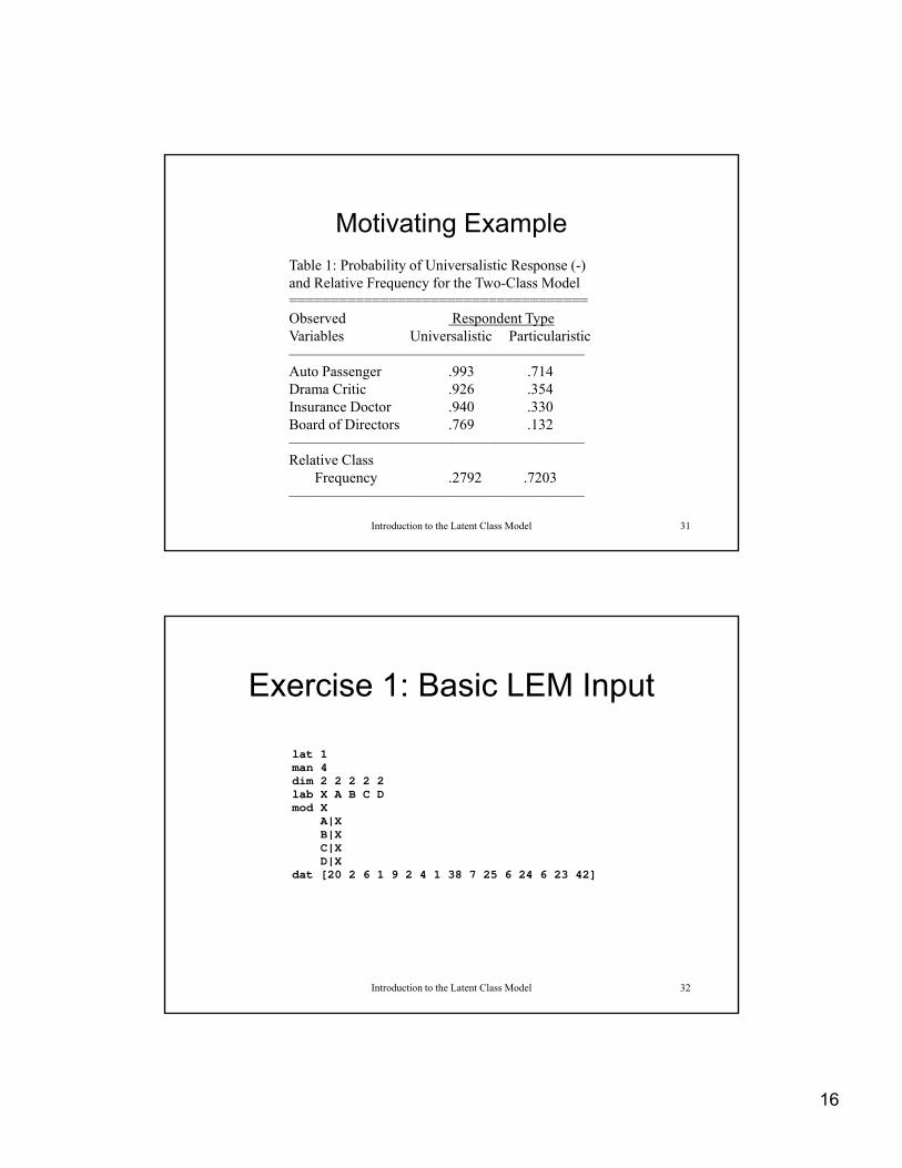
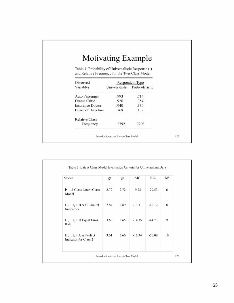
Motivating Example
Table 1: Probability of Universalistic Response (-) and Relative Frequency for the Two-Class Modeland Relative Frequency for the Two Class Model====================================Observed Respondent TypeVariables Universalistic Particularistic————————————————————Auto Passenger .993 .714Drama Critic .926 .354Insurance Doctor .940 .330
d f i
Introduction to the Latent Class Model 10
Board of Directors .769 .132————————————————————Relative Class
Frequency .2792 .7203————————————————————
6
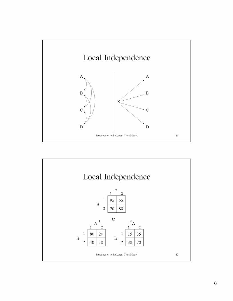
Local Independence
Introduction to the Latent Class Model 11
Local Independence
Introduction to the Latent Class Model 12

7
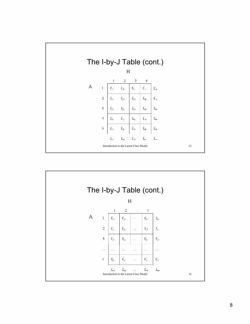
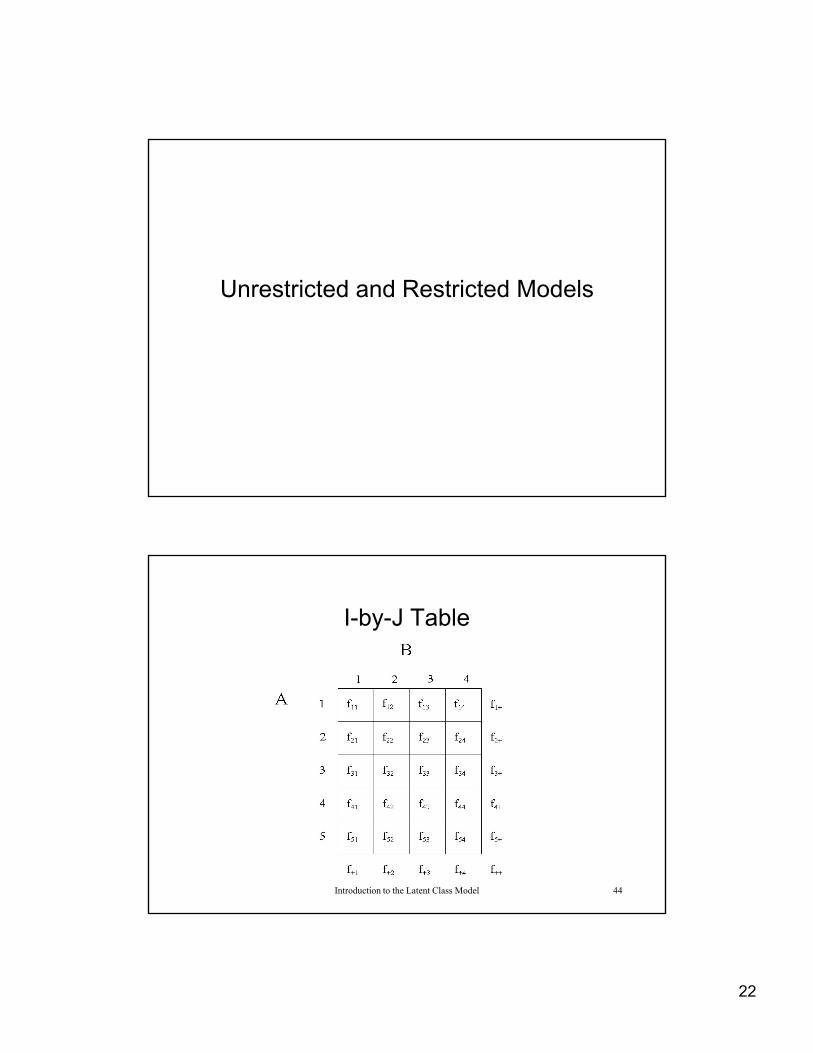
The I-by-J Table
• Assume we have 2 variables, A and B, and that A is causally related to B (i e AB)causally related to B (i.e., AB)
• Further, let “i” index A and “j” index B, where i=1,…,I and j=I,…,J
• For example, if Ai is respondent’s religious identification with, 1=Protestant, 2=Catholic, 3=Jewish, 4=None, 5=Other; (i.e., I=5), then A2 represents the Catholics
Introduction to the Latent Class Model 13
• Let the cell count for the joint distribution of each of the IJ combinations of i and j be represented as fij
The I-by-J Table (cont.)• The resulting I-by-J rectangular display of cell counts
– contingency tablecontingency table– cross-classification table– “crosstabs”
• Frequencies/cell counts (fij) and probabilities (pij)– pij = fij/n, where n is sample size (i.e., total number of observations
[counts] recorded in the contingency table)
• Probability distributions (Agresti uses ij as pop. parameters e se p and ill note sample para )
Introduction to the Latent Class Model 14
parameters, we use pij and will note sample para.)– joint probability (distribution)– marginal probability (distribution)– conditional probability (distribution)
8
The I-by-J Table (cont.)
Introduction to the Latent Class Model 15
The I-by-J Table (cont.)
Introduction to the Latent Class Model 16

9
Probability Distributions
• Joint Probability (distribution)
f 1/
• Marginal Probability (distribution)
ji
ijijij pnfp,
1,/
jjijijj
ii
ji
jijiji
pnfnfpp
pnfnfpp
1,//
1,//
Introduction to the Latent Class Model 17
• Conditional Probability (distribution)
j
ji
ji
ijijj pnfnfpp 1,//
j
ijiijiijij pffppp 1,// ||
Independence
• Two variables are statistically independent when
• Thus, with independence
jiij pppp
p )(
JjandIiforppp jiij ,,1,,1
Introduction to the Latent Class Model 18
ji
ji
i
ijij pppp
|
10
Local Independence
Introduction to the Latent Class Model 19
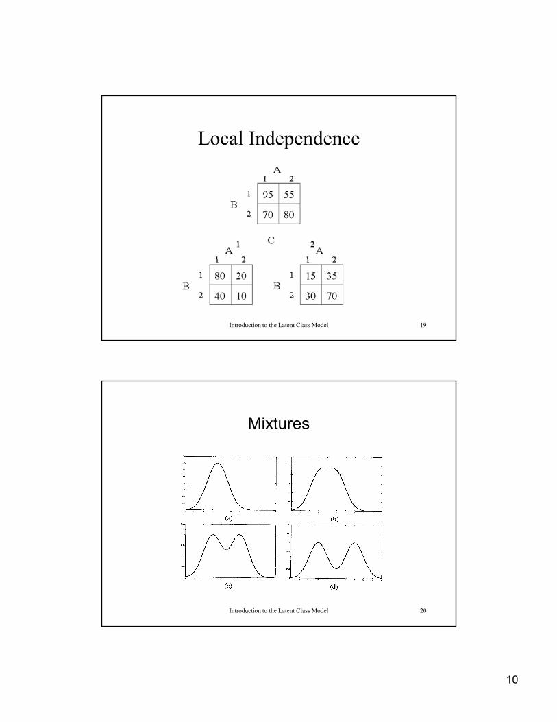
Mixtures
Introduction to the Latent Class Model 20
11
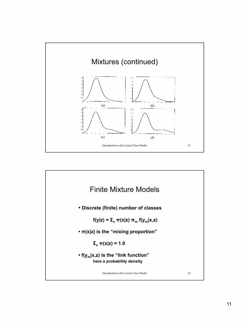
Mixtures (continued)
Introduction to the Latent Class Model 21
Finite Mixture Models
• Discrete (finite) n mber of classes• Discrete (finite) number of classes
f(y|z) = Σx π(x|z) πm f(ym|x,z)
• π(x|z) is the “mixing proportion”
Σ π(x|z) = 1 0
Introduction to the Latent Class Model 22
Σx π(x|z) = 1.0
• f(ym|x,z) is the “link function”here a probability density
12
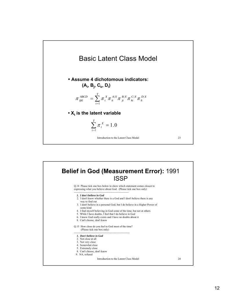
Basic Latent Class Model
• Assume 4 dichotomous indicators: (Ai, Bj, Ck, Dl)
XDlt
XCkt
XBjt
XAit
T
t
Xt
ABCDijkl
||||
1
Introduction to the Latent Class Model 23
• Xt is the latent variable
0.11
T
t
Xt
Belief in God (Measurement Error): 1991 ISSP
Q.14 Please tick one box below to show which statement comes closest toexpressing what you believe about God. (Please tick one box only)-------------------------------------------------------------
1. I don't believe in God 1. I don t believe in God2. I don't know whether there is a God and I don't believe there is any
way to find out3. I don't believe in a personal God, but I do believe in a Higher Power of
some kind 4. I find myself believing in God some of the time, but not at others 5. While I have doubts, I feel that I do believe in God 6. I know God really exists and I have no doubts about it 8. Can't choose, don't know
Q.15 How close do you feel to God most of the time?(Please tick one box only)
Introduction to the Latent Class Model 24
( y)-------------------------------------------------------------- 1. Don't believe in God 2. Not close at all 3. Not very close 4. Somewhat close 5. Extremely close 8. Can't choose, don't know
9. NA, refused

13
Belief in God (Measurement Error): 1991 ISSP
Q.16 Which best describes your beliefs about God?(Please tick one box only)
-------------------------------------------------- 1. I don't believe in God now and I never have 2. I don't believe in God now, but I used to 3. I believe in God now, but I didn't used to 4. I believe in God now and I always have 8. Can't choose, don't know
9. NA, refused
Introduction to the Latent Class Model 25
Belief in God (Measurement Error):1991 ISSP
Introduction to the Latent Class Model 26

14
Belief in God (Measurement Error): 1991 ISSP
Q14 Q15 Q16 + + + 1272 + + - 582 + - + 5 + - - 113 - + + 25
- + - 45
Introduction to the Latent Class Model 27
+ 45 - - + 9 - - - 781
Motivating Example
1. You are riding in a car driven by a close friend, and he hits a pedestrian. You know that he is going at least 35 miles an hour in a 20-mile-an-hour speed zone There are no otheris going at least 35 miles an hour in a 20 mile an hour speed zone. There are no other witnesses. His lawyer says that if you testify under oath that the speed was only 20 miles an hour, it may save him from serious consequences. What right has your friend to expect you to protect him? (Universalistic: He has no right as a friend to expect me to testify to the lower figure.)
2. As a drama critic, your friend asks you to “go easy on a review” of a bad play in which all of his saving are invested.
3. As a physician, your friend asks you to “shade doubts” about a physical examination for an
Introduction to the Latent Class Model 28
insurance policy.
4. As a member of the board of directors, does your friend have a right to expect that you “tip him off” about financially ruinous, though secret, company information.

15
Motivating Example
16-fold response pattern (2x2x2x2=24)
1 2 3 4 1 2 3 4+ + + + - + + ++ + + - - + + -+ + - + - + - ++ + - - - + - -+ - + + - - + ++ - + - - - + -+ - - + - - - +
Introduction to the Latent Class Model 29
+ - - - - - - -
Motivating Example
Samuel A. Stouffer and Jackson Toby (1951) “R l C fli t d P lit ” A i“Role Conflict and Personality,” American Journal of Sociology 56: 395-406.
1 2 3 4 1 2 3 4+ + + + 20 - + + + 38+ + + - 2 - + + - 7+ + - + 6 - + - + 25+ + - - 1 - + - - 6
Introduction to the Latent Class Model 30
+ - + + 9 - - + + 24+ - + - 2 - - + - 6+ - - + 4 - - - + 23+ - - - 1 - - - - 42
16
Motivating Example
Table 1: Probability of Universalistic Response (-) and Relative Frequency for the Two-Class Modeland Relative Frequency for the Two Class Model====================================Observed Respondent TypeVariables Universalistic Particularistic————————————————————Auto Passenger .993 .714Drama Critic .926 .354Insurance Doctor .940 .330
d f i
Introduction to the Latent Class Model 31
Board of Directors .769 .132————————————————————Relative Class
Frequency .2792 .7203————————————————————
Exercise 1: Basic LEM Input
lat 1 man 4 dim 2 2 2 2 2 lab X A B C D mod X A|X B|X C|X D|X dat [20 2 6 1 9 2 4 1 38 7 25 6 24 6 23 42]
Introduction to the Latent Class Model 32
17
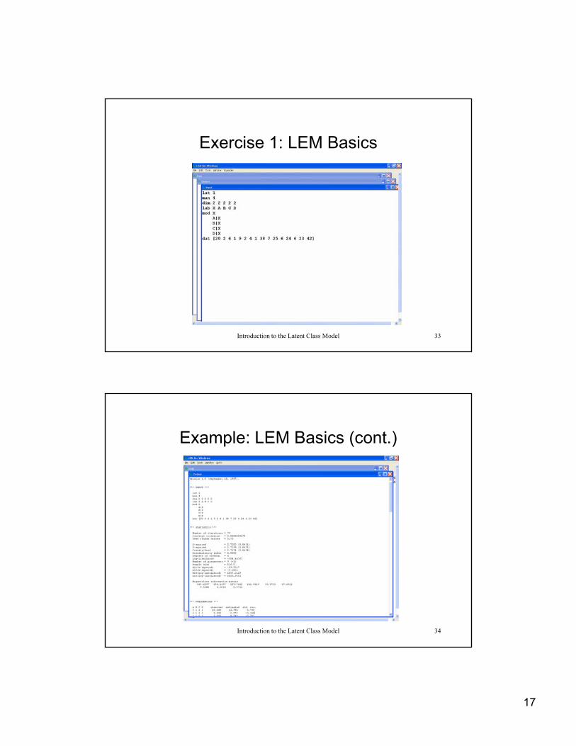
Exercise 1: LEM Basics
Introduction to the Latent Class Model 33
Example: LEM Basics (cont.)
Introduction to the Latent Class Model 34

18
*** STATISTICS ***
Number of iterations = 77Converge criterion = 0.0000009747Seed random values = 4741
X-squared = 2.7200 (0.8431)L-squared = 2.7199 (0.8431)Cressie-Read = 2.7174 (0.8434)Dissimilarity index = 0.0386Degrees of freedom = 6Log-likelihood = -504.46767Number of parameters = 9 (+1)Sample size = 216.0BIC(L-squared) = -29.5317AIC(L-squared) = -9.2801BIC(log likelihood) 1057 3129
Introduction to the Latent Class Model 35
BIC(log-likelihood) = 1057.3129AIC(log-likelihood) = 1026.9353
Eigenvalues information matrix263.6368 254.1479 237.7647 141.9316 93.3723 27.6927
9.5250 5.2903 0.5734
*** FREQUENCIES ***
A B C D observed estimated std. res.1 1 1 1 20.000 16.758 0.7921 1 1 2 2.000 2.557 -0.3481 1 2 1 6.000 8.243 -0.7811 1 2 2 1.000 1.278 -0.2461 1 2 2 1.000 1.278 0.2461 2 1 1 9.000 9.186 -0.0611 2 1 2 2.000 1.418 0.4891 2 2 1 4.000 4.596 -0.2781 2 2 2 1.000 0.965 0.0362 1 1 1 38.000 41.804 -0.5882 1 1 2 7.000 6.570 0.1682 1 2 1 25.000 21.475 0.7612 1 2 2 6.000 6.315 -0.1252 2 1 1 24.000 23.643 0.073
^
^
f
ff
Introduction to the Latent Class Model 36
2 2 1 2 6.000 6.064 -0.0262 2 2 1 23.000 23.294 -0.0612 2 2 2 42.000 41.834 0.026

19
*** (CONDITIONAL) PROBABILITIES ***
* P(X) *
1 0.2794 (0.0581)2 0.7206 (0.0581)
* P(A|X) *
1 | 1 0.0068 (0.0253)2 | 1 0 9932 (0 0253)
Xt
)(| XAXA l2 | 1 0.9932 (0.0253)1 | 2 0.2865 (0.0404)2 | 2 0.7135 (0.0404)
* P(B|X) *
1 | 1 0.0736 (0.0656)2 | 1 0.9264 (0.0656)1 | 2 0.6461 (0.0486)2 | 2 0.3539 (0.0486)
* P(C|X) *
)(| XAit
XAit also
XBjt
|
Introduction to the Latent Class Model 37
1 | 1 0.0604 (0.0660)2 | 1 0.9396 (0.0660)1 | 2 0.6705 (0.0497)2 | 2 0.3295 (0.0497)
* P(D|X) *
1 | 1 0.2310 (0.0952)2 | 1 0.7690 (0.0952)1 | 2 0.8677 (0.0383)2 | 2 0.1323 (0.0383)
XCkt
|
XDlt
|
Motivating ExampleTable 1: Probability of Universalistic Response (-) and Relative Frequency for the Two-Class Modeland Relative Frequency for the Two Class Model====================================Observed Respondent TypeVariables Universalistic Particularistic————————————————————Auto Passenger .993 .714Drama Critic .926 .354Insurance Doctor .940 .330
d f i
Introduction to the Latent Class Model 38
Board of Directors .769 .132————————————————————Relative Class
Frequency .2792 .7203————————————————————

20
How do you calculate the expected (f-hat)?
And
XDlt
XCkt
XBjt
XAit
Xt
ABCDXijklt
||||
XDXCXBXAXT
ABCD ||||
So, for example, for response pattern 2, 1, 2, 1, we have
XDlt
XCkt
XBjt
XAit
Xt
t
ABCDijkl
||||
1
2310.*9396.*0736.*9932.*2794.21211 ABCDX
Introduction to the Latent Class Model 39
0044330.21211
0949758.
8677.*3295.*6461.*7135.*7206.21212
ABCDX
And, thus
0994088.2121 ABCD
4723.21216*094088.*2121
^
2121 Nf ABCD
2 1 1 2 7.000 6.570 0.168 2 1 2 1 25.000 21.475 0.761 2 1 2 2 6.000 6.315 -0.125
Modal Probabilities:
0445936
0994088.004433.212121211|
12121 ABCDABCDXABCDX
Introduction to the Latent Class Model 40
0445936.
9554064.
0994088.0949758.212121212|
22121
ABCDABCDXABCDX

21
Exercise 1: Mplus Basics
TITLE: this is an example of a LCM using the Stouffer and Toby dataLCM using the Stouffer and Toby data
that has two latent classes and uses automatic start values with
random startsMpLCA1
DATA: FILE IS c:\workshops\utdallas05\lca1.dat;VARIABLE: NAMES ARE u1-u4;
CLASSES = c (2);CATEGORICAL = u1-u4;
Introduction to the Latent Class Model 41
ANALYSIS: TYPE = MIXTURE;OUTPUT: TECH1 TECH8;
Exercise 1: Mplus Basics (cont.)1 1 1 1 LCA1.dat
1 1 1 1
1 1 1 1
1 1 1 1
1 1 1 1
1 1 1 1
1 1 1 1
1 1 1 1
1 1 1 1
1 1 1 1
1 1 1 1
1 1 1 1
1 1 1 1
1 1 1 1
1 1 1 1
1 1 1 1
1 1 1 1
Introduction to the Latent Class Model 42
1 1 1 1
1 1 1 1
1 1 1 1
1 1 1 1
1 1 1 2
1 1 1 2
1 1 2 1
1 1 2 1
…
22
Unrestricted and Restricted Models
I-by-J Table
Introduction to the Latent Class Model 44
23
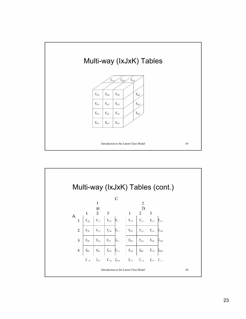
Multi-way (IxJxK) Tables
Introduction to the Latent Class Model 45
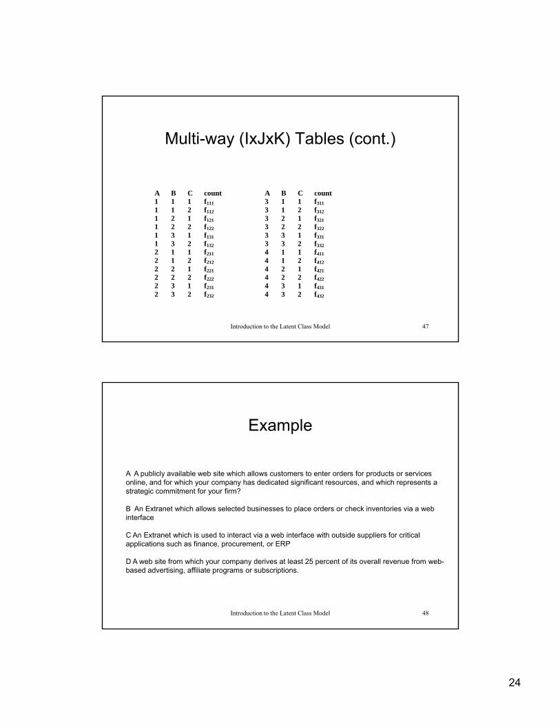
Multi-way (IxJxK) Tables (cont.)
Introduction to the Latent Class Model 46
24
Multi-way (IxJxK) Tables (cont.)
A B C count1 1 1 f111
1 1 2 f112
1 2 1 f121
1 2 2 f122
1 3 1 f131
1 3 2 f132
2 1 1 f211
2 1 2 f
A B C count3 1 1 f311
3 1 2 f312
3 2 1 f321
3 2 2 f322
3 3 1 f331
3 3 2 f332
4 1 1 f411
4 1 2 f
Introduction to the Latent Class Model 47
2 1 2 f212
2 2 1 f221
2 2 2 f222
2 3 1 f231
2 3 2 f232
4 1 2 f412
4 2 1 f421
4 2 2 f422
4 3 1 f431
4 3 2 f432
Example
A A publicly available web site which allows customers to enter orders for products or services online, and for which your company has dedicated significant resources, and which represents a strategic commitment for your firm?
B An Extranet which allows selected businesses to place orders or check inventories via a web interface
C An Extranet which is used to interact via a web interface with outside suppliers for critical applications such as finance, procurement, or ERP
Introduction to the Latent Class Model 48
pp , p ,
D A web site from which your company derives at least 25 percent of its overall revenue from web-based advertising, affiliate programs or subscriptions.

25
Multi-way Response Table as Array
A B C D count 1 1 1 1 2 1 1 1 2 12 1 1 2 1 1
1 1 2 2 11 1 2 1 1 0 1 2 1 2 8 1 2 2 1 3
A B C D count 2 1 1 1 0 2 1 1 2 3 2 1 2 1 0
2 1 2 2 9 2 2 1 1 1 2 2 1 2 17 2 2 2 1 5
Introduction to the Latent Class Model 49
1 2 2 2 42 2 2 2 2 147
Exercise 2: Basic LEM Input
* Unrestricted latent class model* A = Web site allows customer orders A Web site allows customer orders* B = Extranet allows selected business to* place orders, etc.* C = Extranet which is used to interacct w/* outside suppliers* D = Web site from which company derives at* least 25% revenue
lat 1man 4dim 2 2 2 2 2
Introduction to the Latent Class Model 50
dim 2 2 2 2 2lab X A B C Dmod X A|X B|X C|X D|Xdat [2 12 1 11 0 8 3 42 0 3 0 9 1 17 5 147 ]see 79144

26
*** STATISTICS ***
Number of iterations = 104Converge criterion = 0.0000008765Seed random values = 79144
X-squared = 2.5470 (0.8632)L d 3 5306 (0 7399)L-squared = 3.5306 (0.7399)Cressie-Read = 2.7190 (0.8432)Dissimilarity index = 0.0174Degrees of freedom = 6Log-likelihood = -406.73333Number of parameters = 9 (+1)Sample size = 261.0BIC(L-squared) = -29.8566AIC(L-squared) = -8.4694BIC(log-likelihood) = 863.5473
Introduction to the Latent Class Model 51
BIC(log likelihood) 863.5473AIC(log-likelihood) = 831.4667
Eigenvalues information matrix292.3539 157.9235 93.4596 63.9076 58.5344 34.063519.9269 6.7323 3.1609
*** FREQUENCIES ***
A B C D observed estimated std. res.1 1 1 1 2.000 1.444 0.4631 1 1 2 12.000 12.600 -0.1691 1 2 1 1.000 1.092 -0.0881 1 2 2 11.000 10.848 0.0461 2 1 1 0.000 0.477 -0.6911 2 1 2 8.000 7.374 0.2301 2 2 1 3.000 1.839 0.8561 2 2 2 42.000 43.326 -0.2012 1 1 1 0.000 0.225 -0.4742 1 1 2 3.000 2.538 0.2902 1 2 1 0.000 0.435 -0.6602 1 2 2 9.000 8.818 0.0612 2 1 1 1 000 0 719 0 331
Introduction to the Latent Class Model 52
2 2 1 1 1.000 0.719 0.3312 2 1 2 17.000 17.623 -0.1482 2 2 1 5.000 5.769 -0.3202 2 2 2 147.000 145.873 0.093
27
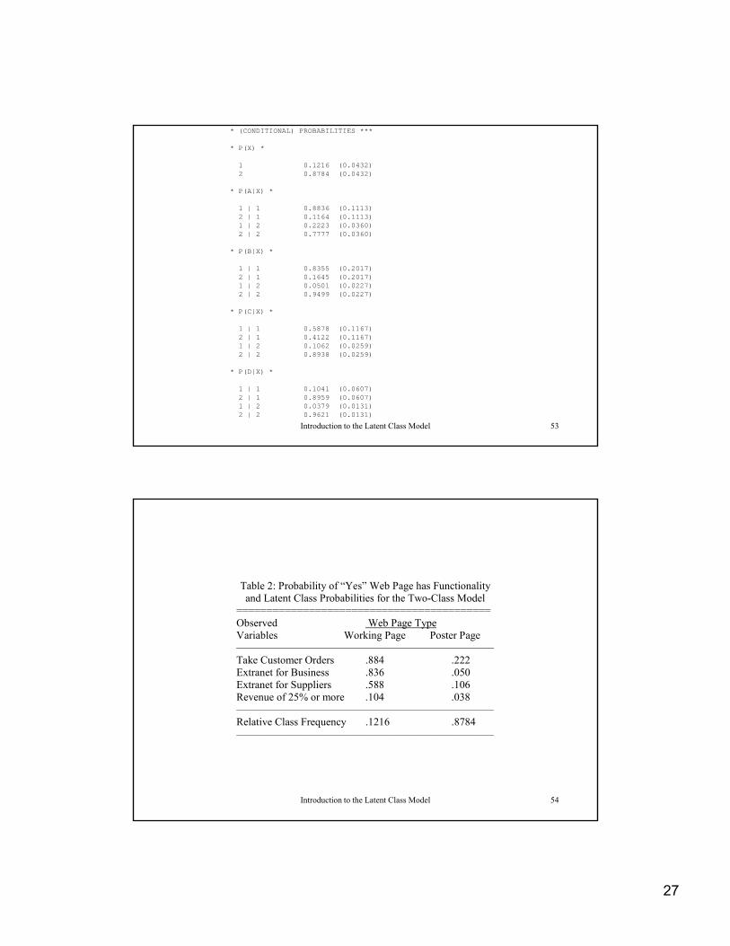
* (CONDITIONAL) PROBABILITIES ***
* P(X) *
1 0.1216 (0.0432)2 0.8784 (0.0432)
* P(A|X) *
1 | 1 0.8836 (0.1113)2 | 1 0.1164 (0.1113)1 | 2 0.2223 (0.0360)2 | 2 0 7777 (0 0360)2 | 2 0.7777 (0.0360)
* P(B|X) *
1 | 1 0.8355 (0.2017)2 | 1 0.1645 (0.2017)1 | 2 0.0501 (0.0227)2 | 2 0.9499 (0.0227)
* P(C|X) *
1 | 1 0.5878 (0.1167)2 | 1 0.4122 (0.1167)
Introduction to the Latent Class Model 53
| ( )1 | 2 0.1062 (0.0259)2 | 2 0.8938 (0.0259)
* P(D|X) *
1 | 1 0.1041 (0.0607)2 | 1 0.8959 (0.0607)1 | 2 0.0379 (0.0131)2 | 2 0.9621 (0.0131)
Table 2: Probability of “Yes” Web Page has Functionalityand Latent Class Probabilities for the Two-Class Model
==========================================Observed Web Page TypeVariables Working Page Poster Page————————————————————————Take Customer Orders .884 .222Extranet for Business .836 .050Extranet for Suppliers .588 .106Revenue of 25% or more .104 .038————————————————————————
Introduction to the Latent Class Model 54
Relative Class Frequency .1216 .8784————————————————————————
28
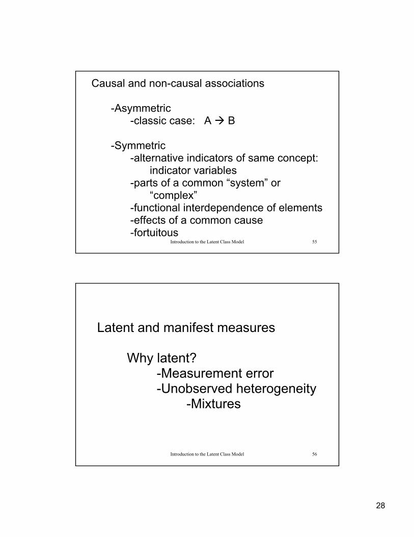
Causal and non-causal associations -Asymmetric -classic case: A B -Symmetric -alternative indicators of same concept:
indicator variables -parts of a common “system” or
“ l ”
Introduction to the Latent Class Model 55
“complex” -functional interdependence of elements -effects of a common cause -fortuitous
Latent and manifest measures Why latent? -Measurement error -Unobserved heterogeneity
-Mixtures
Introduction to the Latent Class Model 56
-Mixtures
29
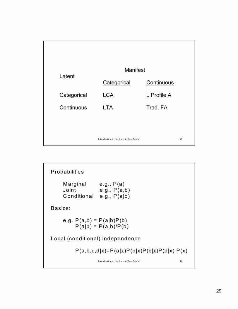
Manifest LatentLatent
Categorical Continuous
Categorical LCA L Profile A
Continuous LTA Trad. FA
Introduction to the Latent Class Model 57
Probabilities Marginal e.g., P(a) Joint e.g., P(a,b) Conditional e.g., P(a|b)g , ( | ) Basics:
e.g. P(a,b) = P(a|b)P(b) P(a|b) = P(a,b)/P(b)
Introduction to the Latent Class Model 58
Local (conditional) Independence P(a,b,c,d|x)=P(a|x)P(b|x)P(c|x)P(d|x) P(x)
30
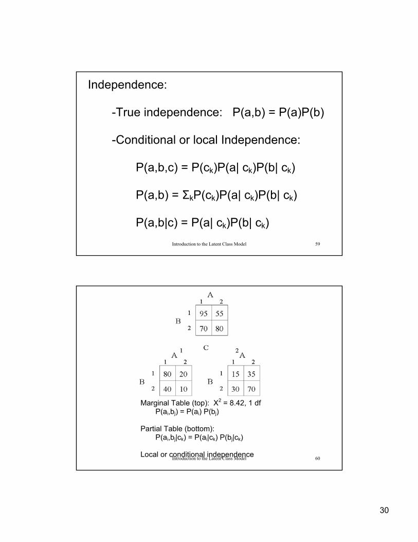
Independence: -True independence: P(a,b) = P(a)P(b) -Conditional or local Independence:
P(a,b,c) = P(ck)P(a| ck)P(b| ck) P(a b) = Σ P(c )P(a| c )P(b| c )
Introduction to the Latent Class Model 59
P(a,b) = ΣkP(ck)P(a| ck)P(b| ck) P(a,b|c) = P(a| ck)P(b| ck)
Marginal Table (top): X2 = 8.42, 1 df P( b ) P( ) P(b )
Introduction to the Latent Class Model 60
P(ai,bj) = P(ai) P(bj) Partial Table (bottom): P(ai,bj|ck) = P(ai|ck) P(bj|ck) Local or conditional independence
31
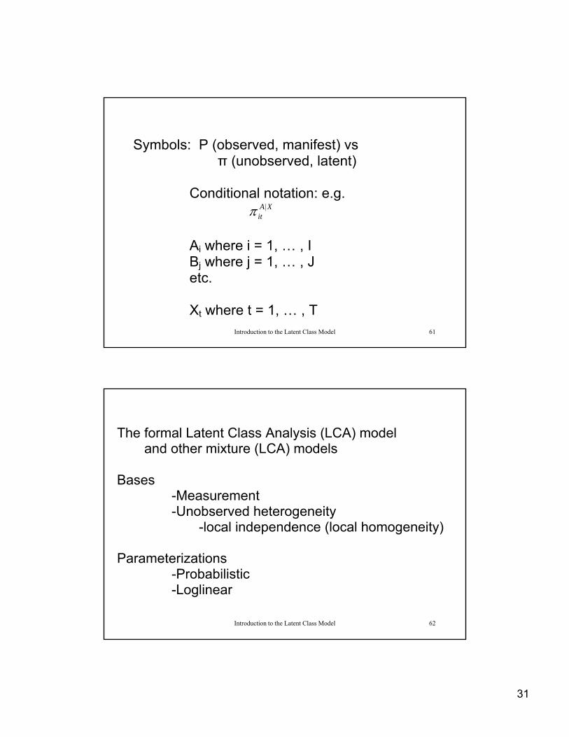
Symbols: P (observed, manifest) vs π (unobserved, latent)
Conditional notation: e.g.
Ai where i = 1, … , I
Bj where j = 1 J
XAit
|
Introduction to the Latent Class Model 61
Bj where j 1, … , J etc. Xt where t = 1, … , T
The formal Latent Class Analysis (LCA) model and other mixture (LCA) models
Bases
-Measurement -Unobserved heterogeneity -local independence (local homogeneity) Parameterizations
Introduction to the Latent Class Model 62
Parameterizations -Probabilistic -Loglinear

32
Formal Latent Class Model
XDlt
XCkt
XBjt
XAit
T
t
Xt
ABCDijkl
||||
1
Where
is the latent class, or “mixing,” probabilities, and
Xt
Introduction to the Latent Class Model 63
are the conditional probabilities linking each of the indicator variables to the latent variable (Xt).
XDlt
XCkt
XBjt
XAit and |||| ,,,
It fo llow s tha t
W here
ABCDijklijkl NF *
^
W hen the re a re fou r ind ica to r va riab les (A i, B j, C k, D l).
I
i
J
j
K
k
L
lijklFN
1 1 1 1
Introduction to the Latent Class Model 64
T h is can be genera lized to any num ber o f ind ica to r va riab les . T he cu rren t exam p les w ill assum e fou r ind ica to r va riab les .
33
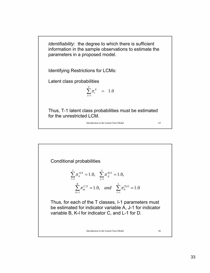
Identifiability: the degree to which there is sufficient information in the sample observations to estimate the parameters in a proposed model. Identifying Restrictions for LCMs: Latent class probabilities
0.11
T
t
Xt
Introduction to the Latent Class Model 65
Thus, T-1 latent class probabilities must be estimated for the unrestricted LCM.
Conditional probabilities
0101 || J
XBI
XA
Thus, for each of the T classes, I-1 parameters must b ti t d f i di t i bl A J 1 f i di t
0.1,0.1
,0.1,0.1
1
|
1
|
11
L
l
XDlt
K
k
XCkt
jjt
iit
and
Introduction to the Latent Class Model 66
be estimated for indicator variable A, J-1 for indicator variable B, K-l for indicator C, and L-1 for D.
34
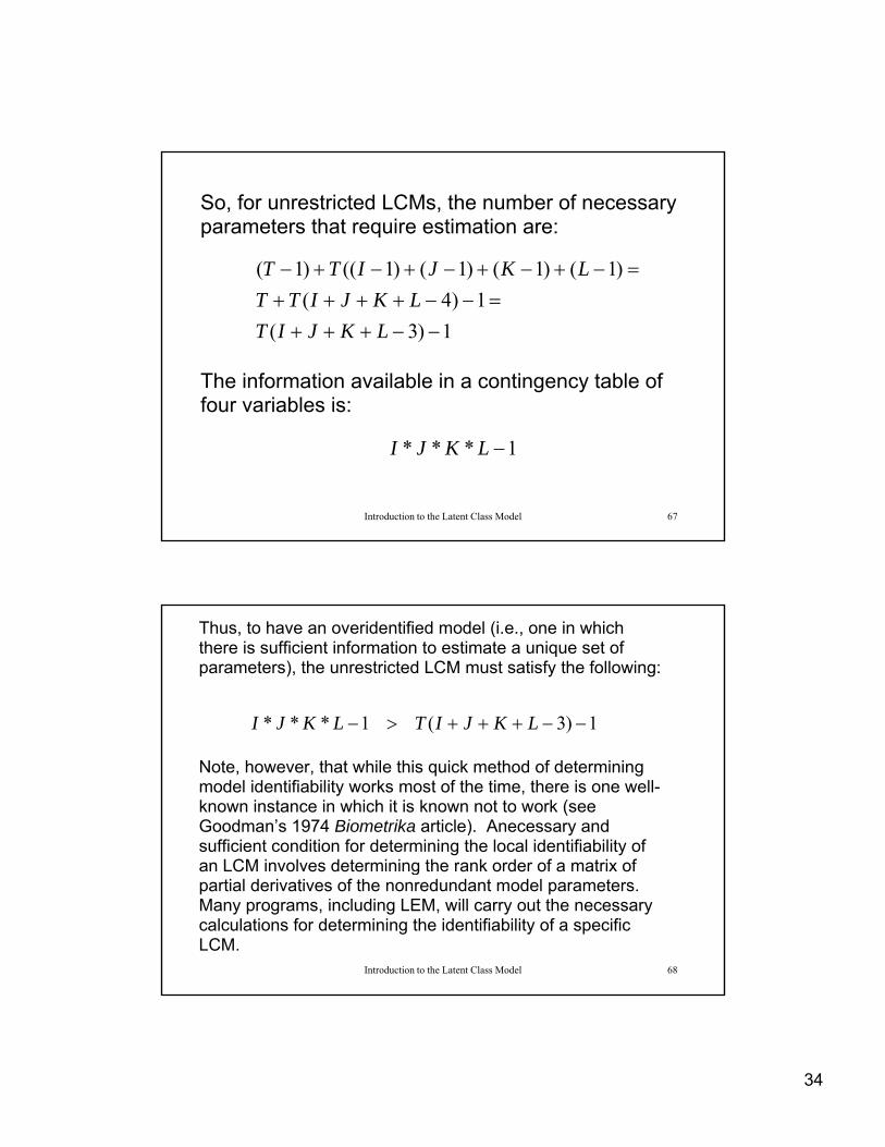
So, for unrestricted LCMs, the number of necessary parameters that require estimation are:
)1()1()1()1(()1( LKJITT
The information available in a contingency table of four variables is:
1)3(
1)4(
LKJIT
LKJITT
Introduction to the Latent Class Model 67
four variables is:
1*** LKJI
Thus, to have an overidentified model (i.e., one in which there is sufficient information to estimate a unique set of parameters), the unrestricted LCM must satisfy the following:
1)3(1*** LKJITLKJI Note, however, that while this quick method of determining model identifiability works most of the time, there is one well-known instance in which it is known not to work (see Goodman’s 1974 Biometrika article). Anecessary and sufficient condition for determining the local identifiability of an LCM involves determining the rank order of a matrix of
Introduction to the Latent Class Model 68
an LCM involves determining the rank order of a matrix of partial derivatives of the nonredundant model parameters. Many programs, including LEM, will carry out the necessary calculations for determining the identifiability of a specific LCM.
35
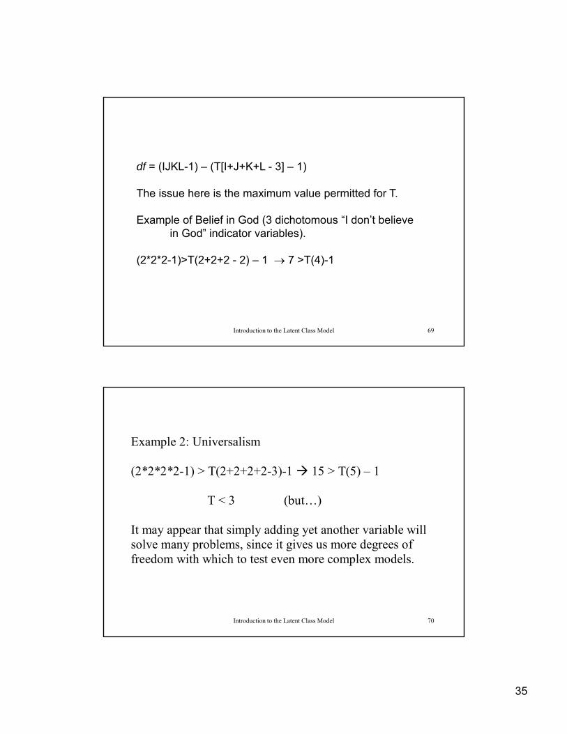
df = (IJKL-1) – (T[I+J+K+L - 3] – 1)
The issue here is the maximum value permitted for T.
Example of Belief in God (3 dichotomous “I don’t believe in God” indicator variables).
(2*2*2-1)>T(2+2+2 - 2) – 1 7 >T(4)-1
Introduction to the Latent Class Model 69
(2 2 2 1) T(2 2 2 2) 1 7 T(4) 1
Example 2: Universalism
(2*2*2*2 1) > T(2+2+2+2 3) 1 15 > T(5) 1(2*2*2*2-1) > T(2+2+2+2-3)-1 15 > T(5) – 1
T < 3 (but…)
It may appear that simply adding yet another variable willsolve many problems, since it gives us more degrees of
Introduction to the Latent Class Model 70
freedom with which to test even more complex models.

36
Motivating ExampleTable 1: Probability of Universalistic Response (-) and Relative Frequency for the Two-Class Modeland Relative Frequency for the Two Class Model====================================Observed Respondent TypeVariables Universalistic Particularistic————————————————————Auto Passenger .993 .714Drama Critic .926 .354Insurance Doctor .940 .330
d f i
Introduction to the Latent Class Model 71
Board of Directors .769 .132————————————————————Relative Class
Frequency .2792 .7203————————————————————
Sparseness: many sampling zeros in observed dataset. Latent Class Models (and loglinear models) are caseLatent Class Models (and loglinear models) are case intensive—they require relatively large sample sizes. All two-variable, three-variable and higher-order parameters are modeled, thus these models are information (i.e., sample size) intensive. S l d t diffi lti i d l l ti
Introduction to the Latent Class Model 72
Sparseness leads to difficulties in model evaluation; specifically, to determining the number of degrees of freedom for the model test (Agresti, 1990, Categorical Data Analysis).

37
Resampling methods such as jack-knifing and boot-strapping, however, can be used to evaluate parameters (see Langeheineevaluate parameters (see Langeheine, Pannekoek and Van de Pol, 1996, SMR) PANMARK provides bootstrap estimates of standard errors for LCM parameters estimated from sparse data tables.
Introduction to the Latent Class Model 73
p
Maximum likelihood estimation (mle) of latent class model parameters is through iterative estimation procedures: EM (expectation maximization; see McCutcheon 1987) or Newton-Raphson, or some variant of these two (see Vermunt, 1997, Log-Linear Models for Event Histories, esp. App. A, C, D)
Introduction to the Latent Class Model 74

38
Boundary Estimates
Introduction to the Latent Class Model 75
Model Evaluation Pearson Chi-Square
ijklijkl FFX ^
2^
2 )(
Likelihood Ratio Chi-Square
ijkl
ijklF^
ijklijkl
FFG ^
2 ln2
Introduction to the Latent Class Model 76
Where
ijkl
ijkl
ijkl
F
ABCDijklijkl NF *
^

39
Information criteria Akaike Information Criteria (AIC)
Bayesian Information Criteria (BIC)
dfGAIC 22
)][ln(*2 NdfGBIC
Introduction to the Latent Class Model 77
Prefer lowest negative value for AIC and BIC.
)][ln(* NdfGBIC
Evaluation Criteria X-squared = 2.7200 (0.8431) L-squared = 2.7199 (0.8431) Cressie-Read = 2.7174 (0.8434) Number of parameters = 9 (+1) Sample size = 216.0 BIC(L-squared) = -29.5317
Introduction to the Latent Class Model 78
( q ) AIC(L-squared) = -9.2801

40
Restricted Latent Class Models
Hypothesis Testing
-Equality restrictions-Equality restrictions-Deterministic restrictions
-Conditional probabilities-Latent class probabilities
Equality Restrictions on Conditional Probabilities
Introduction to the Latent Class Model 79
The parallel indicators hypothesis (e.g.)
XCXBXCXB and |12
|12
|11
|11
Motivating ExampleTable 1: Probability of Universalistic Response (-) and Relative Frequency for the Two-Class Modeland Relative Frequency for the Two Class Model====================================Observed Respondent TypeVariables Universalistic Particularistic————————————————————Auto Passenger .993 .714Drama Critic .926 .354Insurance Doctor .940 .330
d f i
Introduction to the Latent Class Model 80
Board of Directors .769 .132————————————————————Relative Class
Frequency .2792 .7203————————————————————
41
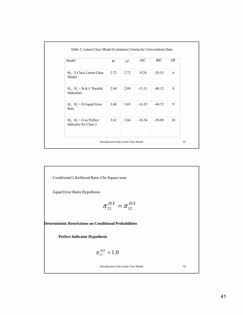
Table 2: Latent Class Model Evaluation Criteria for Universalism Data
Model X2 G2 AIC BIC DF
H1: 2-Class Latent Class Model
2.72 2.72 -9.28 -29.53 6Model
H2: H1 + B & C Parallel Indicators
2.84 2.89 -13.11 -40.12 8
H3: H2 + D Equal Error Rate
3.60 3.65 -14.35 -44.73 9
Introduction to the Latent Class Model 81
H4: H3 + A as Perfect Indicator for Class 2
3.61 3.66 -16.34 -50.09 10
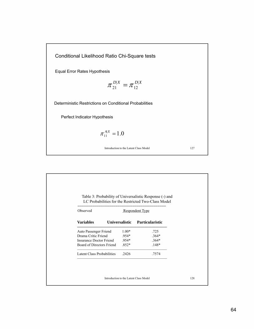
Conditional Likelihood Ratio Chi-Square tests
Equal Error Rates Hypothesis
XDXD |12
|21
Deterministic Restrictions on Conditional Probabilities
Perfect Indicator Hypothesis
Introduction to the Latent Class Model 82
0.1|11 XA
Perfect Indicator Hypothesis
42
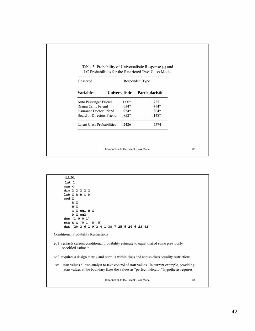
Table 3: Probability of Universalistic Response (-) and LC Probabilities for the Restricted Two-Class Model
==========================================Observed Respondent TypeObserved Respondent Type
Variables Universalistic Particularistic————————————————————————Auto Passenger Friend 1.00* .725Drama Critic Friend .954* .364*Insurance Doctor Friend .954* .364*Board of Directors Friend .852* .148*
Introduction to the Latent Class Model 83
————————————————————————Latent Class Probabilities .2426 .7574————————————————————————
LEMlat 1man 4 dim 2 2 2 2 2lab X A B C Dmod X
A|X B|X C|X eq1 B|X| q |D|X eq2
des [1 0 0 1]sta A|X [0 1 .5 .5]dat [20 2 6 1 9 2 4 1 38 7 25 6 24 6 23 42]
Conditional Probability Restrictions
eq1 restricts current conditional probability estimate to equal that of some previouslyspecified estimate
Introduction to the Latent Class Model 84
p
eq2 requires a design matrix and permits within class and across class equality restrictions
sta start values allows analyst to take control of start values. In current example, providingstart values at the boundary fixes the values as “perfect indicator” hypothesis requires.

43
Mplus Specification for H4TITLE: this is an example of a LCM using the Stouffer and Toby data which has
two latent classes and the restrictions implied by Hypothesis 4MpLCA2
DATA: FILE IS c:\workshops\utdallas05\lca1.dat;VARIABLE: NAMES ARE u1 u4;VARIABLE: NAMES ARE u1-u4;
CLASSES = c (2);CATEGORICAL = u1-u4;
ANALYSIS: TYPE = MIXTURE;MODEL:
%OVERALL%%c#1%[u1$1*-1];[u2$1*-1] (1);[u3$1*-1] (1);[u4$1*-1] (p1);
Introduction to the Latent Class Model 85
%c#2%[u1$1@-15];[u2$1*1] (2);[u3$1*1] (2);[u4$1*1] (p2);
MODEL CONSTRAINT:p2 = - p1;
OUTPUT: TECH1 TECH8;
Model Selection and Evaluation

44
Some Basic Concepts
• Maximum likelihood principle– “In effect this principle says that when faced with severalIn effect this principle says that when faced with several
parameter values, any of which might be the true one for the population, the best ‘bet’ is that parameter value which would have made the sample actually obtained have the highest prior probability. When in doubt, place your bet on that parameter value which would have made the obtained result most likely.” (Hays, 1981, pg. 182)
• Sampling distribution assumed
Introduction to the Latent Class Model 87
• Sampling distribution assumed– multinomial sampling– independent (product) multinomial sampling
Sampling Distributions
• Poisson samplingPoisson sampling– counts (ni) assumed as random variables
– total sample size (n) is random variable
• Multinomial sampling– total sample size (n) is fixed
– random sampling
– ni are conditioned on n; they can not exceed n
Introduction to the Latent Class Model 88
ni are conditioned on n; they can not exceed n
– Σini = n
inii
ii
i nn
nnP
!!
)|(
45
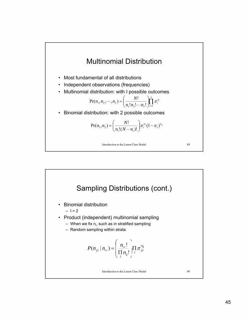
Multinomial Distribution
• Most fundamental of all distributionsMost fundamental of all distributions
• Independent observations (frequencies)
• Multinomial distribution: with I possible outcomes
• Binomial distribution: with 2 possible outcomes
I
i
ni
II
i
nnn
Nnnn
12121 !!!
!),,,Pr(
Introduction to the Latent Class Model 89
p
2)1()!(!
!),Pr( 1
1121
nni
i
nNn
Nnn
Sampling Distributions (cont.)
• Binomial distributionBinomial distribution – I = 2
• Product (independent) multinomial sampling– When we fix ni, such as in stratified sampling
– Random sampling within strata
Introduction to the Latent Class Model 90
ijn
ijjijj
iiij n
nnnP || !
!)|(
46
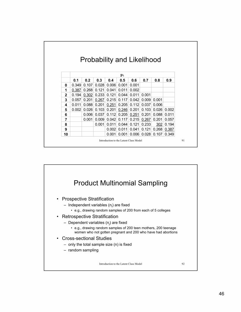
Probability and Likelihood
p10.1 0.2 0.3 0.4 0.5 0.6 0.7 0.8 0.9
0 0.349 0.107 0.028 0.006 0.001 0.0011 0.387 0.268 0.121 0.041 0.011 0.0022 0.194 0.302 0.233 0.121 0.044 0.011 0.0013 0.057 0.201 0.267 0.215 0.117 0.042 0.009 0.0014 0.011 0.088 0.201 0.251 0.205 0.112 0.037 0.0065 0.002 0.026 0.103 0.201 0.246 0.201 0.103 0.026 0.002
p
Introduction to the Latent Class Model 91
6 0.006 0.037 0.112 0.205 0.251 0.201 0.088 0.0117 0.001 0.009 0.042 0.117 0.215 0.267 0.201 0.0578 0.001 0.011 0.044 0.121 0.233 302 0.1949 0.002 0.011 0.041 0.121 0.268 0.387
10 0.001 0.001 0.006 0.028 0.107 0.349
Product Multinomial Sampling
• Prospective StratificationProspective Stratification – Independent variables (ni) are fixed
• e.g., drawing random samples of 200 from each of 5 colleges
• Retrospective Stratification– Dependent variables (nj) are fixed
• e.g., drawing random samples of 200 teen mothers, 200 teenage women who not gotten pregnant and 200 who have had abortions
Introduction to the Latent Class Model 92
• Cross-sectional Studies– only the total sample size (n) is fixed
– random sampling

47
Maximum likelihood estimation (mle) of latent class model parameters is through iterative estimation procedures: EM (expectation maximization; see McCutcheon 1987) or Newton-Raphson, or some variant of these two (see Vermunt, 1997, Log-Linear Models for Event Histories, esp. App. A, C, D)
Introduction to the Latent Class Model 93
Maximum Likelihood
• Given the observed data the likelihood function isGiven the observed data, the likelihood function is the probability of ni for the sampling model, treated as an unknown set of parameters
• The factorials of the multinomial are constants, so the kernel of the probability function is
ini
Introduction to the Latent Class Model 94
• Maximize the log of the ML (monotonic function), log of the likelihood
ii
iinL log

48
Maximum likelihood (cont.)
• Differentiate L with respect to πi givesDifferentiate L with respect to πi gives
• The ML solution satisfies πi/πI = ni/nI
0
I
I
i
i
i
nnL
I
I
I
iIi n
nn
n ˆ)(ˆ
1ˆ
Introduction to the Latent Class Model 95
• So, πI = nI/n and πi = ni/n = pi
• For contingency tables, the ML estimates of cell probabilities are the sample cell proportions
II nn
Boundary Estimates
Introduction to the Latent Class Model 96
49
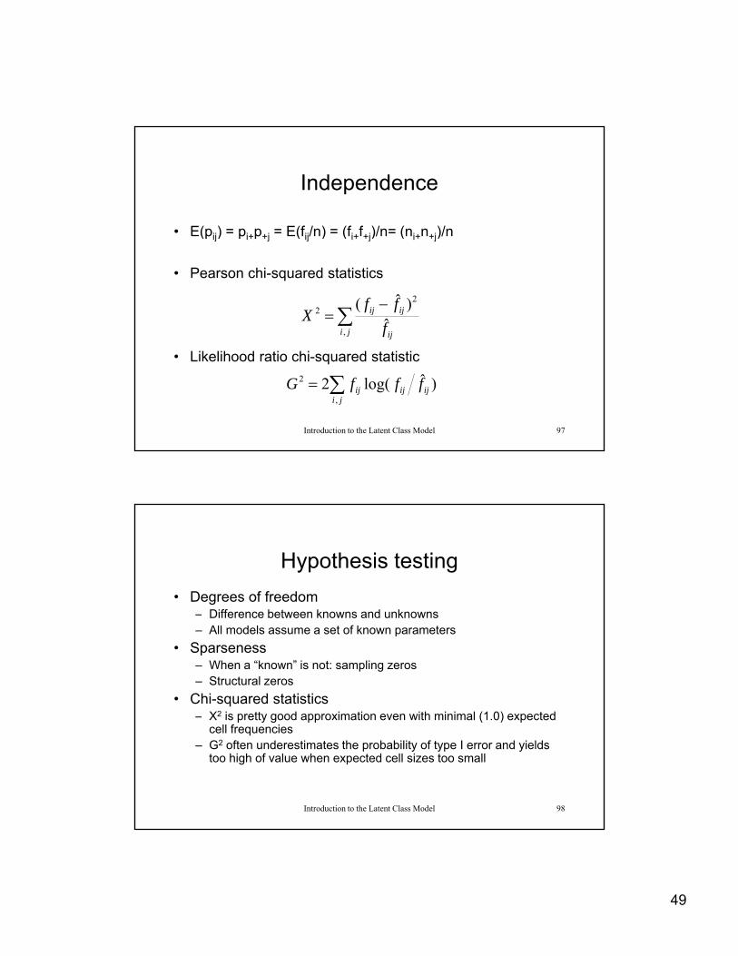
Independence
• E(pij) = pi+p+j = E(fij/n) = (fi+f+j)/n= (ni+n+j)/nE(pij) pi+p+j E(fij/n) (fi+f+j)/n (ni+n+j)/n
• Pearson chi-squared statistics
ji ij
ijij
f
ffX
,
22
ˆ)ˆ(
Introduction to the Latent Class Model 97
• Likelihood ratio chi-squared statistic
)ˆlog(2,
2ijij
jiij fffG
Hypothesis testing
• Degrees of freedomDifference between knowns and unknowns– Difference between knowns and unknowns
– All models assume a set of known parameters
• Sparseness– When a “known” is not: sampling zeros– Structural zeros
• Chi-squared statistics– X2 is pretty good approximation even with minimal (1.0) expected
Introduction to the Latent Class Model 98
p y g pp ( ) pcell frequencies
– G2 often underestimates the probability of type I error and yields too high of value when expected cell sizes too small
50
Identifiability: the degree to which there is sufficient information in the sample observations to estimate the parameters in a proposed model. Identifying Restrictions for LCMs: Latent class probabilities
0.11
T
t
Xt
Introduction to the Latent Class Model 99
Thus, T-1 latent class probabilities must be estimated for the unrestricted LCM.
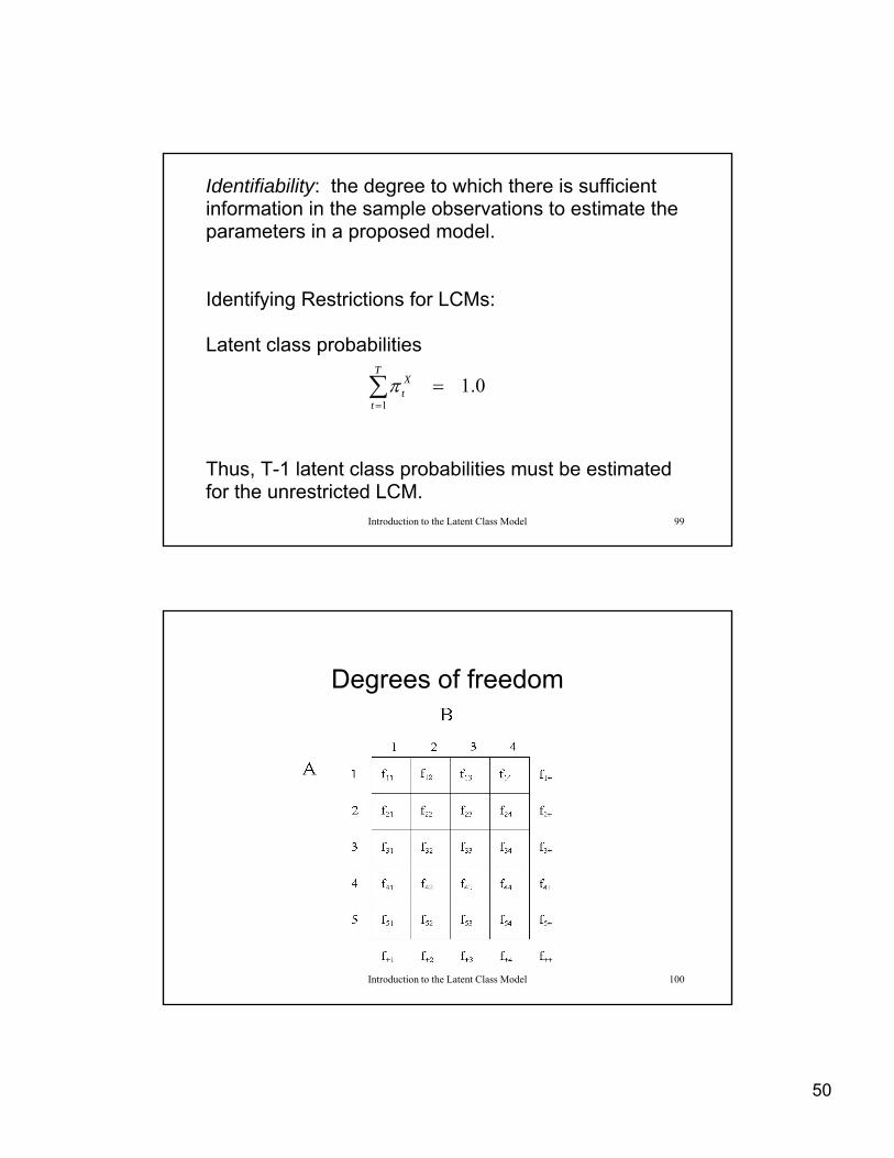
Degrees of freedom
Introduction to the Latent Class Model 100

51
Degrees of Freedom (cont.)
• Knowns (data)– In the I x J contingency table: IJ
• Unknowns (parameters)– Sample size (n) is fixed, so we lose 1 df: (IJ-1)
– Independence: I-1 row marginals and J-1 column marginals
– Odds ratios (I-1)(J-1)
– IJ = 1 + [(I-1) + (J-1)] + [(I-1)(J-1)]
Introduction to the Latent Class Model 101
• DF= (IJ-1) - estimated parameters– Independence model: df = (I-1)(J-1)
• Identifiability and Model Identification
Degrees of Freedom
• How many “knowns” do we have?How many knowns do we have?– For the ABCD table, we have (IJKL)-1
• How many (unique) parameters are we estimating?– Recall the identifying restrictions (e.g., I-1, [I-1][J-1], etc.)
• DF = (IJKL-1) - # of estimated parameters
Introduction to the Latent Class Model 102
52
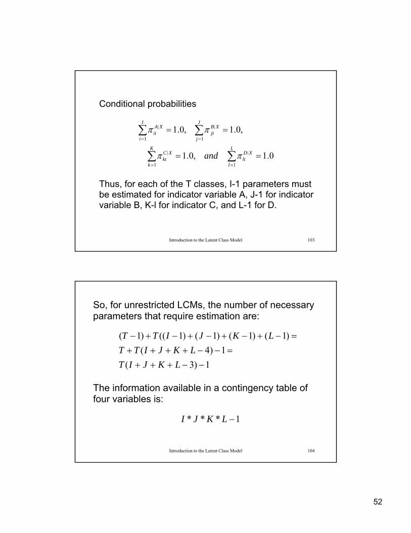
Conditional probabilities
0101 || J
XBI
XA
Thus, for each of the T classes, I-1 parameters must b ti t d f i di t i bl A J 1 f i di t
0.1,0.1
,0.1,0.1
1
|
1
|
11
L
l
XDlt
K
k
XCkt
jjt
iit
and
Introduction to the Latent Class Model 103
be estimated for indicator variable A, J-1 for indicator variable B, K-l for indicator C, and L-1 for D.
So, for unrestricted LCMs, the number of necessary parameters that require estimation are:
)1()1()1()1(()1( LKJITT
The information available in a contingency table of four variables is:
1)3(
1)4(
LKJIT
LKJITT
Introduction to the Latent Class Model 104
four variables is:
1*** LKJI

53
Thus, to have an overidentified model (i.e., one in which there is sufficient information to estimate a unique set of parameters), the unrestricted LCM must satisfy the following:
1)3(1*** LKJITLKJI Note, however, that while this quick method of determining model identifiability works most of the time, there is one well-known instance in which it is known not to work (see Goodman’s 1974 Biometrika article). Anecessary and sufficient condition for determining the local identifiability of an LCM involves determining the rank order of a matrix of
Introduction to the Latent Class Model 105
an LCM involves determining the rank order of a matrix of partial derivatives of the nonredundant model parameters. Many programs, including LEM, will carry out the necessary calculations for determining the identifiability of a specific LCM.
df = (IJKL-1) – (T[I+J+K+L - 3] – 1)
The issue here is the maximum value permitted for T.
Example of Belief in God (3 dichotomous “I don’t believe in God” indicator variables).
(2*2*2-1)>T(2+2+2 - 2) – 1 7 >T(4)-1
Introduction to the Latent Class Model 106
(2 2 2 1) T(2 2 2 2) 1 7 T(4) 1

54
Example 2: Universalism
(2*2*2*2 1) > T(2+2+2+2 3) 1 15 > T(5) 1(2*2*2*2-1) > T(2+2+2+2-3)-1 15 > T(5) – 1
T < 3 (but…)
It may appear that simply adding yet another variable willsolve many problems, since it gives us more degrees of
Introduction to the Latent Class Model 107
freedom with which to test even more complex models.
Sparseness: many sampling zeros in observed dataset. Latent Class Models (and loglinear models) are caseLatent Class Models (and loglinear models) are case intensive—they require relatively large sample sizes. All two-variable, three-variable and higher-order parameters are modeled, thus these models are information (i.e., sample size) intensive. S l d t diffi lti i d l l ti
Introduction to the Latent Class Model 108
Sparseness leads to difficulties in model evaluation; specifically, to determining the number of degrees of freedom for the model test (Agresti, 1990, Categorical Data Analysis).
55
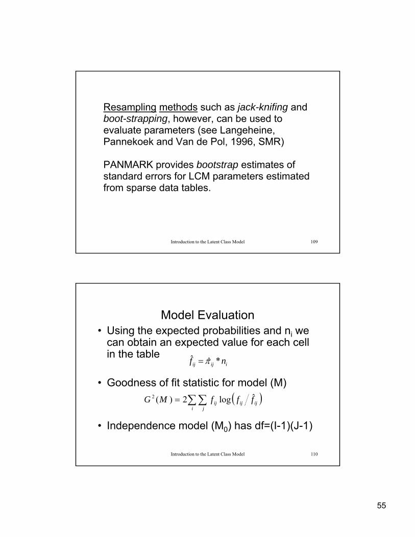
Resampling methods such as jack-knifing and boot-strapping, however, can be used to evaluate parameters (see Langeheineevaluate parameters (see Langeheine, Pannekoek and Van de Pol, 1996, SMR) PANMARK provides bootstrap estimates of standard errors for LCM parameters estimated from sparse data tables.
Introduction to the Latent Class Model 109
p
Model Evaluation• Using the expected probabilities and ni we
can obtain an expected value for each cellcan obtain an expected value for each cell in the table
• Goodness of fit statistic for model (M)
iijij nf *ˆˆ
ijijij fffMG ˆlog2)(2
Introduction to the Latent Class Model 110
• Independence model (M0) has df=(I-1)(J-1)
i j
jjj

56
Calculating Expected Cell Counts
• Basic latent class modelXDXCXBXAXABCDX ||||
• Expected cell proportions
ltktjtittijklt||||
T
XDlt
XCkt
XBjt
XAit
Xt
ABCDijkl
||||
Introduction to the Latent Class Model 111
• Expected cell counts
t
jj1
nf ABCDijklijkl *ˆ
Model Evaluation (cont.)
• Conditional chi-square (G2) testing:Conditional chi square (G ) testing:
)()(
)](2[)(2
)(2)|(
12
22
22
12122
MGMG
LLLL
LLMMG
ss
Introduction to the Latent Class Model 112
• L2 must be “nested” within L1 to use conditional chi-square testing

57
Model Diagnostics
• Standardized residuals ˆStandardized residuals
• Diagnostics for GLMs
ij
ijijij
f
ffe
ˆ
ˆ
0
0
LLL
D M
Introduction to the Latent Class Model 113
)()()(
02
20
2*
0
MGMGMG
D
L
Evaluation Criteria
• Pearson goodness of fit Chi-square statisticPearson goodness of fit Chi square statistic
• Likelihood Ratio goodness of fit Chi-square statistic– Also, conditional L2 statistic
• Information Criteria– Akaike Information Criteria (AIC)
dfGAIC 22
Introduction to the Latent Class Model 114
– Bayesian Information Criteria (BIC)
)][ln(*2 ndfGBIC
58
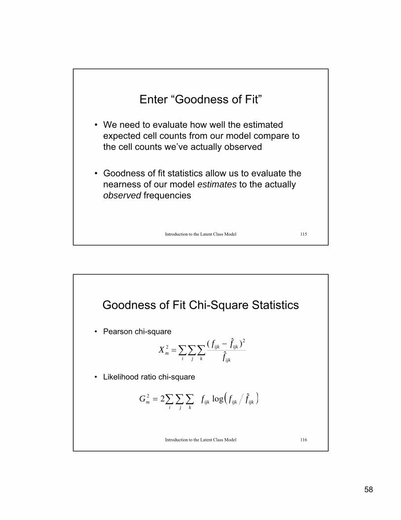
Enter “Goodness of Fit”
• We need to evaluate how well the estimatedWe need to evaluate how well the estimated expected cell counts from our model compare to the cell counts we’ve actually observed
• Goodness of fit statistics allow us to evaluate the nearness of our model estimates to the actually
Introduction to the Latent Class Model 115
nearness of our model estimates to the actually observed frequencies
Goodness of Fit Chi-Square Statistics
• Pearson chi-squarePearson chi square
• Likelihood ratio chi-square
i j k ijk
ijkijkm f
ffX ˆ
)ˆ( 22
Introduction to the Latent Class Model 116
i j
ijkijkijkk
m fffG ˆlog22

59
Conditional Chi-Square Testing
• Assume we have a model M1 that fits the observed dataAssume we have a model M1 that fits the observed data
• This is distributed as chi-square with degrees of freedom)()(
)](2[)(2
)(2)|(
12
22
22
12122
MGMG
LLLL
LLMMG
ss
Introduction to the Latent Class Model 117
q g
)()()|( 1212 MdfMdfMMdf
Conditional Chi-Square Test• Conditional chi-square for M2|M1: 17.8104 – 1.0247 =
16.785716.7857• Degrees of freedom for M2|M1: 9 - 2 = 7• Probability: p = .0188• Decision: reject M2
• Conditional chi-square for M3|M1: 7.9333 – 1.0247 = 6.9086
Introduction to the Latent Class Model 118
• Degrees of freedom for M3|M1: 7 - 2 = 5• Probability: p = .2275• Decision: accept M3

60
Iterative ML Estimation
• Iterative Proportional Fitting (IPF)Iterative Proportional Fitting (IPF)– Start with initial estimates– Apply scaling factor– Successively adjust expected values until convergence
• Newton-Raphson– Start with initial estimates
Introduction to the Latent Class Model 119
– Approximate function in neighborhood of guess by a second-degree function
– Successive approximations of second-degree functions until convergence
Motivating ExampleTable 1: Probability of Universalistic Response (-) and Relative Frequency for the Two-Class Modeland Relative Frequency for the Two Class Model====================================Observed Respondent TypeVariables Universalistic Particularistic————————————————————Auto Passenger .993 .714Drama Critic .926 .354Insurance Doctor .940 .330
d f i
Introduction to the Latent Class Model 120
Board of Directors .769 .132————————————————————Relative Class
Frequency .2792 .7203————————————————————
61
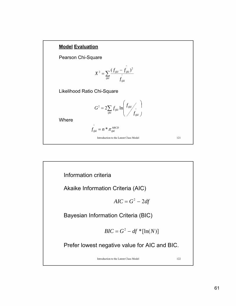
Model Evaluation Pearson Chi-Square
ijklijkl ffX ^
2^
2 )(
Likelihood Ratio Chi-Square
ijkl
ijklf^
ijklijkl
ffG ^
2 ln2
Introduction to the Latent Class Model 121
Where
ijkl
ijkl
ijkl
ff
ABCDijklijkl nf *
^
Information criteria Akaike Information Criteria (AIC)
Bayesian Information Criteria (BIC)
dfGAIC 22
)][ln(*2 NdfGBIC
Introduction to the Latent Class Model 122
Prefer lowest negative value for AIC and BIC.
)][ln(* NdfGBIC

62
Evaluation Criteria X-squared = 2.7200 (0.8431) L-squared = 2.7199 (0.8431) Cressie-Read = 2.7174 (0.8434) Number of parameters = 9 (+1) Sample size = 216.0 BIC(L-squared) = -29.5317
Introduction to the Latent Class Model 123
( q ) AIC(L-squared) = -9.2801
Restricted Latent Class Models
Hypothesis Testing
-Equality restrictions-Equality restrictions-Deterministic restrictions
-Conditional probabilities-Latent class probabilities
Equality Restrictions on Conditional Probabilities
Introduction to the Latent Class Model 124
The parallel indicators hypothesis (e.g.)
XCXBXCXB and |12
|12
|11
|11
63
Motivating ExampleTable 1: Probability of Universalistic Response (-) and Relative Frequency for the Two-Class Modeland Relative Frequency for the Two Class Model====================================Observed Respondent TypeVariables Universalistic Particularistic————————————————————Auto Passenger .993 .714Drama Critic .926 .354Insurance Doctor .940 .330
d f i
Introduction to the Latent Class Model 125
Board of Directors .769 .132————————————————————Relative Class
Frequency .2792 .7203————————————————————
Table 2: Latent Class Model Evaluation Criteria for Universalism Data
Model X2 G2 AIC BIC DF
H1: 2-Class Latent Class Model
2.72 2.72 -9.28 -29.53 6Model
H2: H1 + B & C Parallel Indicators
2.84 2.89 -13.11 -40.12 8
H3: H2 + D Equal Error Rate
3.60 3.65 -14.35 -44.73 9
Introduction to the Latent Class Model 126
H4: H3 + A as Perfect Indicator for Class 2
3.61 3.66 -16.34 -50.09 10
64
Conditional Likelihood Ratio Chi-Square tests
Equal Error Rates Hypothesis
XDXD |12
|21
Deterministic Restrictions on Conditional Probabilities
Perfect Indicator Hypothesis
Introduction to the Latent Class Model 127
0.1|11 XA
Perfect Indicator Hypothesis
Table 3: Probability of Universalistic Response (-) and LC Probabilities for the Restricted Two-Class Model
==========================================Observed Respondent TypeObserved Respondent Type
Variables Universalistic Particularistic————————————————————————Auto Passenger Friend 1.00* .725Drama Critic Friend .954* .364*Insurance Doctor Friend .954* .364*Board of Directors Friend .852* .148*
Introduction to the Latent Class Model 128
————————————————————————Latent Class Probabilities .2426 .7574————————————————————————

65
LEMlat 1man 4 dim 2 2 2 2 2lab X A B C Dmod X
A|X B|X C|X eq1 B|X| q |D|X eq2
des [1 0 0 1]sta A|X [0 1 .5 .5]dat [20 2 6 1 9 2 4 1 38 7 25 6 24 6 23 42]
Conditional Probability Restrictions
eq1 restricts current conditional probability estimate to equal that of some previouslyspecified estimate
Introduction to the Latent Class Model 129
p
eq2 requires a design matrix and permits within class and across class equality restrictions
sta start values allows analyst to take control of start values. In current example, providingstart values at the boundary fixes the values as “perfect indicator” hypothesis requires.
Scale Analysis

66
Scaling Items with LCM’s
• Assumes underlying latent continuum• Assumes underlying latent continuum– Ability (e.g., mathematics, verbal)
– Attitudes (e.g., racism, ethnocentrism)
• Dichotomous items of varying difficulty
• LCA can be restricted to introduce
Introduction to the Latent Class Model 131
LCA can be restricted to introduce probabilistic model of item difficulty and person ability
Item Difficulty
3+4 4*7 22+32 (a+1)(a-3) Low High
Mathematics Scale
Introduction to the Latent Class Model 132

67
Person’s Ability
Low High
A. McCutcheon A. Einstein
Mathematics Scale
Introduction to the Latent Class Model 133
Guttman Scaling Model
A B C D
0 - - - -
1 + - - -
2 + + - -
Introduction to the Latent Class Model 134
3 + + + -
4 + + + +
68
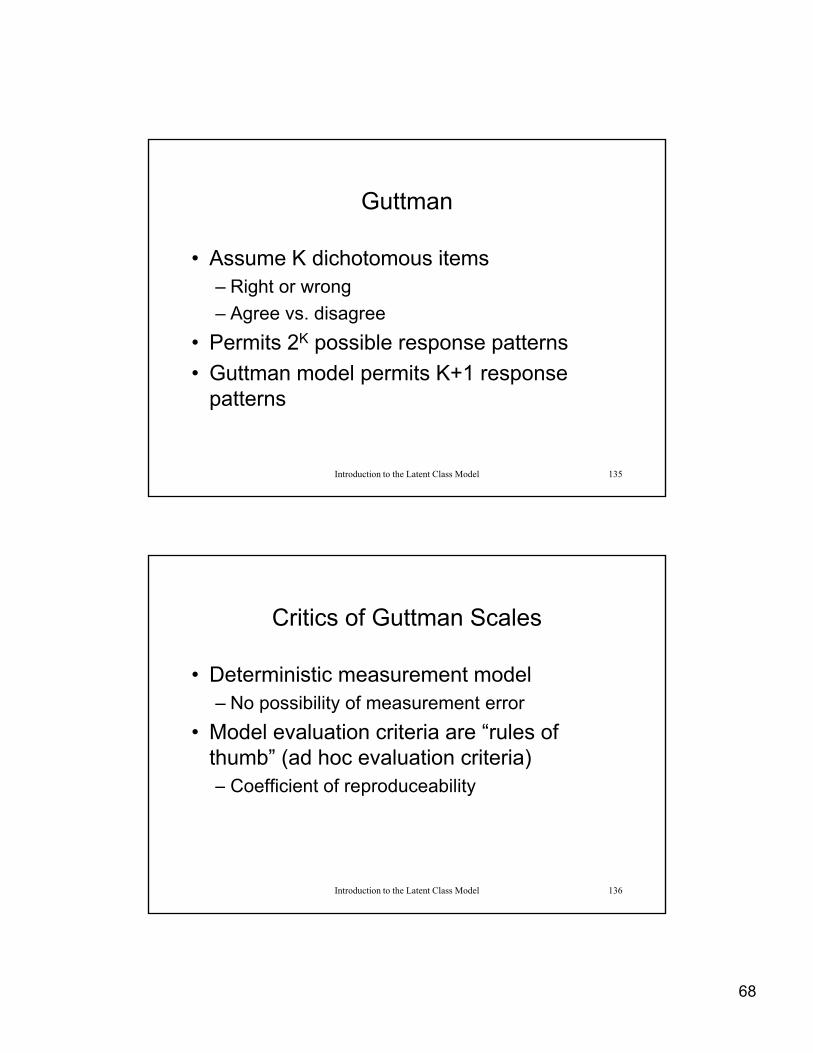
Guttman
• Assume K dichotomous items• Assume K dichotomous items– Right or wrong
– Agree vs. disagree
• Permits 2K possible response patterns
• Guttman model permits K+1 response
Introduction to the Latent Class Model 135
Guttman model permits K 1 response patterns
Critics of Guttman Scales
• Deterministic measurement model• Deterministic measurement model– No possibility of measurement error
• Model evaluation criteria are “rules of thumb” (ad hoc evaluation criteria)– Coefficient of reproduceability
Introduction to the Latent Class Model 136
p y
69
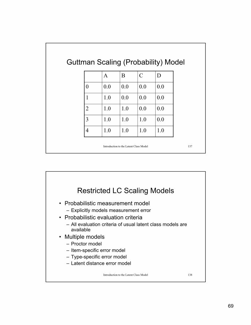
Guttman Scaling (Probability) Model
A B C D
0 0.0 0.0 0.0 0.0
1 1.0 0.0 0.0 0.0
2 1.0 1.0 0.0 0.0
Introduction to the Latent Class Model 137
3 1.0 1.0 1.0 0.0
4 1.0 1.0 1.0 1.0
Restricted LC Scaling Models
• Probabilistic measurement model– Explicitly models measurement error
• Probabilistic evaluation criteria– All evaluation criteria of usual latent class models are
available
• Multiple models– Proctor model
Introduction to the Latent Class Model 138
Proctor model– Item-specific error model– Type-specific error model– Latent distance error model
70
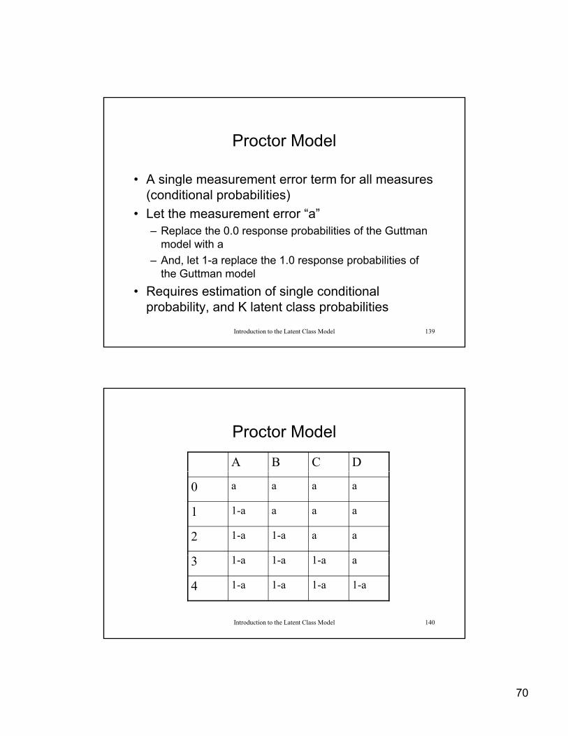
Proctor Model
• A single measurement error term for all measures• A single measurement error term for all measures (conditional probabilities)
• Let the measurement error “a”– Replace the 0.0 response probabilities of the Guttman
model with a
– And, let 1-a replace the 1.0 response probabilities of
Introduction to the Latent Class Model 139
, p p pthe Guttman model
• Requires estimation of single conditional probability, and K latent class probabilities
Proctor Model
A B C D
0 a a a a
1 1-a a a a
2 1-a 1-a a a
Introduction to the Latent Class Model 140
3 1-a 1-a 1-a a
4 1-a 1-a 1-a 1-a
71
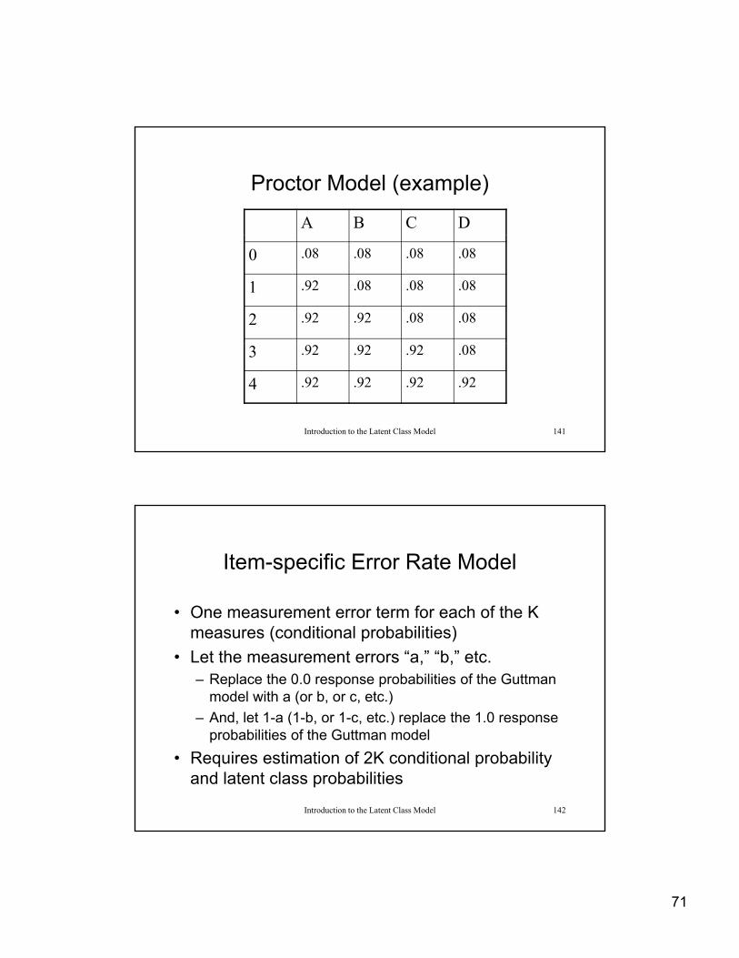
Proctor Model (example)
A B C D
0 .08 .08 .08 .08
1 .92 .08 .08 .08
2 .92 .92 .08 .08
Introduction to the Latent Class Model 141
3 .92 .92 .92 .08
4 .92 .92 .92 .92
Item-specific Error Rate Model
• One measurement error term for each of the K• One measurement error term for each of the K measures (conditional probabilities)
• Let the measurement errors “a,” “b,” etc.– Replace the 0.0 response probabilities of the Guttman
model with a (or b, or c, etc.)
– And, let 1-a (1-b, or 1-c, etc.) replace the 1.0 response
Introduction to the Latent Class Model 142
, ( , , ) p pprobabilities of the Guttman model
• Requires estimation of 2K conditional probability and latent class probabilities
72
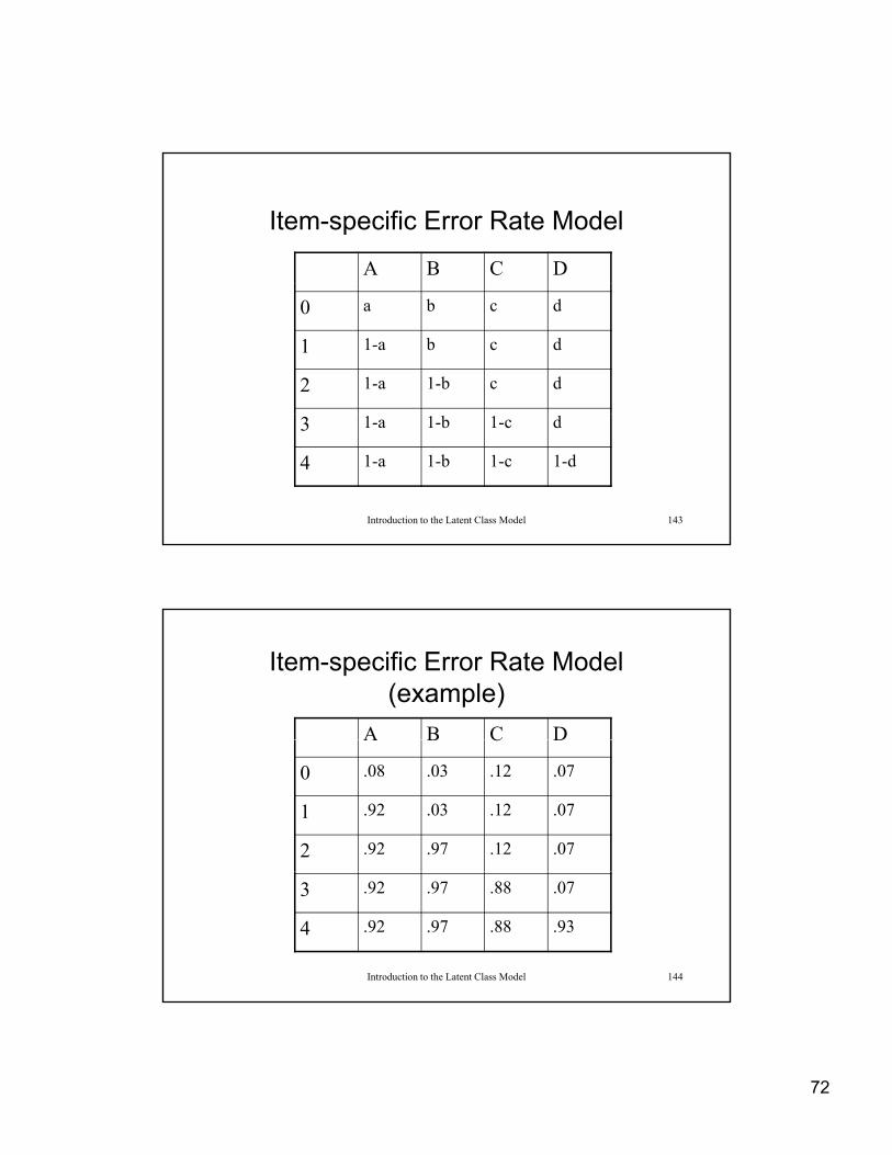
Item-specific Error Rate Model
A B C D
0 a b c d
1 1-a b c d
2 1-a 1-b c d
Introduction to the Latent Class Model 143
3 1-a 1-b 1-c d
4 1-a 1-b 1-c 1-d
Item-specific Error Rate Model (example)
A B C DA B C D
0 .08 .03 .12 .07
1 .92 .03 .12 .07
2 .92 .97 .12 .07
Introduction to the Latent Class Model 144
3 .92 .97 .88 .07
4 .92 .97 .88 .93
73
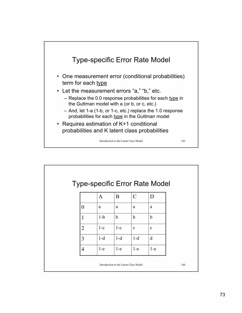
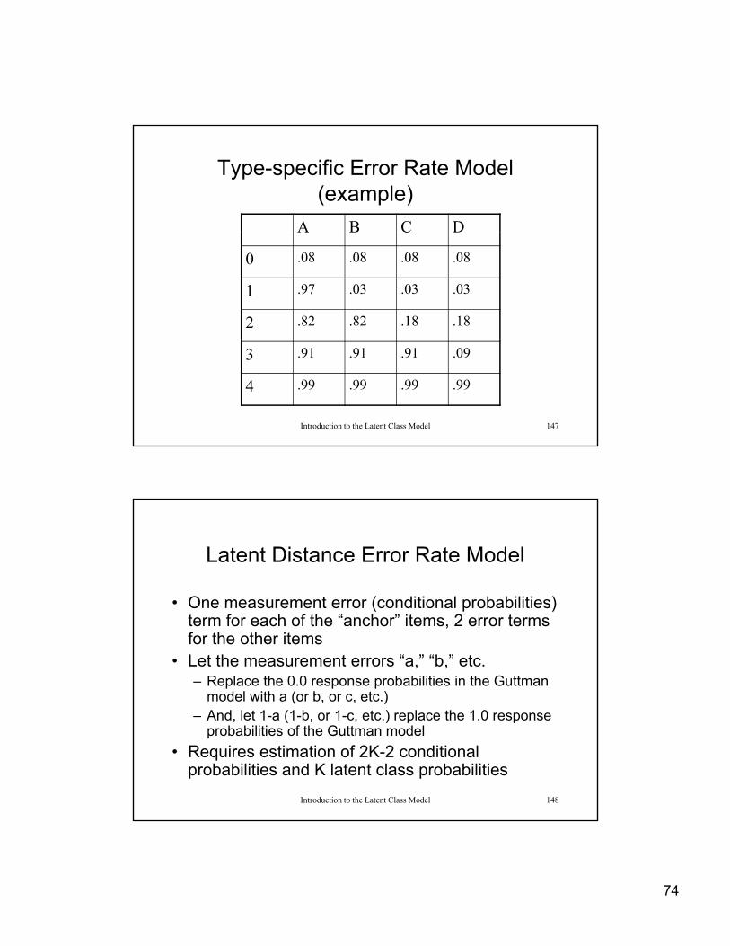
Type-specific Error Rate Model
• One measurement error (conditional probabilities)• One measurement error (conditional probabilities) term for each type
• Let the measurement errors “a,” “b,” etc.– Replace the 0.0 response probabilities for each type in
the Guttman model with a (or b, or c, etc.)
– And, let 1-a (1-b, or 1-c, etc.) replace the 1.0 response
Introduction to the Latent Class Model 145
, ( , , ) p pprobabilities for each type in the Guttman model
• Requires estimation of K+1 conditional probabilities and K latent class probabilities
Type-specific Error Rate Model
A B C D
0 a a a a
1 1-b b b b
2 1-c 1-c c c
Introduction to the Latent Class Model 146
3 1-d 1-d 1-d d
4 1-e 1-e 1-e 1-e
74
Type-specific Error Rate Model (example)
A B C DA B C D
0 .08 .08 .08 .08
1 .97 .03 .03 .03
2 .82 .82 .18 .18
Introduction to the Latent Class Model 147
3 .91 .91 .91 .09
4 .99 .99 .99 .99
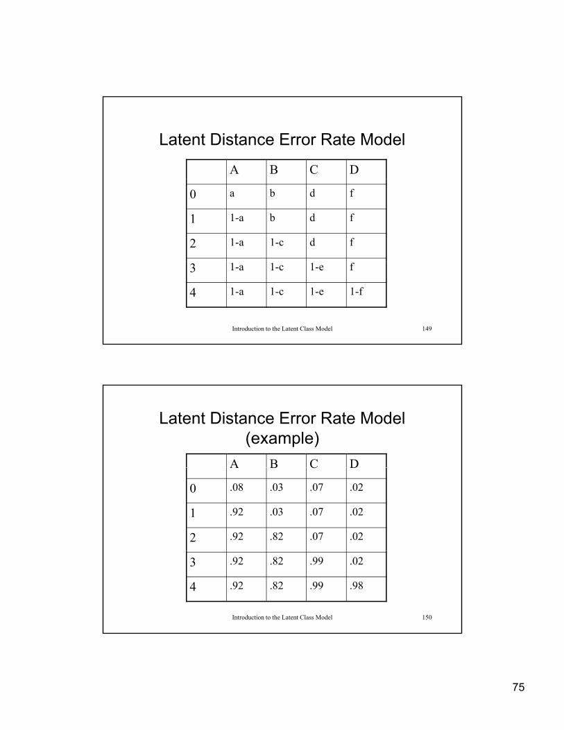
Latent Distance Error Rate Model
• One measurement error (conditional probabilities)One measurement error (conditional probabilities) term for each of the “anchor” items, 2 error terms for the other items
• Let the measurement errors “a,” “b,” etc.– Replace the 0.0 response probabilities in the Guttman
model with a (or b, or c, etc.)And let 1 a (1 b or 1 c etc ) replace the 1 0 response
Introduction to the Latent Class Model 148
– And, let 1-a (1-b, or 1-c, etc.) replace the 1.0 response probabilities of the Guttman model
• Requires estimation of 2K-2 conditional probabilities and K latent class probabilities
75
Latent Distance Error Rate Model
A B C D
0 a b d f
1 1-a b d f
2 1-a 1-c d f
Introduction to the Latent Class Model 149
3 1-a 1-c 1-e f
4 1-a 1-c 1-e 1-f
Latent Distance Error Rate Model (example)
A B C DA B C D
0 .08 .03 .07 .02
1 .92 .03 .07 .02
2 .92 .82 .07 .02
Introduction to the Latent Class Model 150
3 .92 .82 .99 .02
4 .92 .82 .99 .98
76
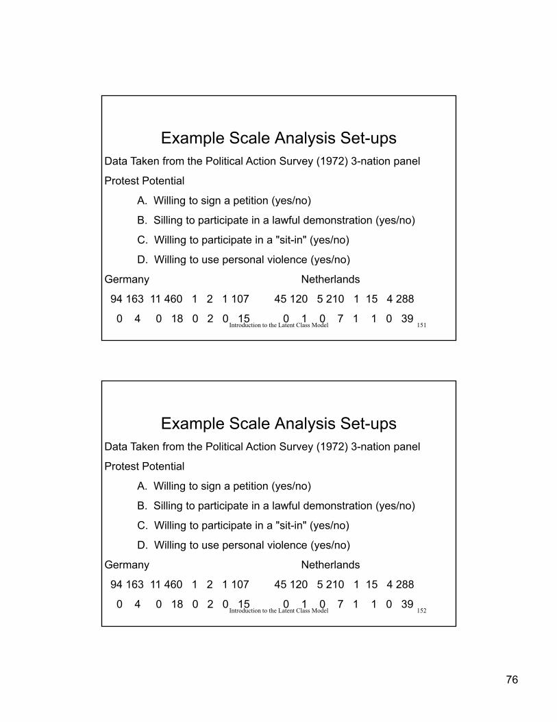
Example Scale Analysis Set-upsData Taken from the Political Action Survey (1972) 3-nation panel
P t t P t ti lProtest Potential
A. Willing to sign a petition (yes/no)
B. Silling to participate in a lawful demonstration (yes/no)
C. Willing to participate in a "sit-in" (yes/no)
D Willing to use personal violence (yes/no)
Introduction to the Latent Class Model 151
D. Willing to use personal violence (yes/no)
Germany Netherlands
94 163 11 460 1 2 1 107 45 120 5 210 1 15 4 288
0 4 0 18 0 2 0 15 0 1 0 7 1 1 0 39
Example Scale Analysis Set-upsData Taken from the Political Action Survey (1972) 3-nation panel
P t t P t ti lProtest Potential
A. Willing to sign a petition (yes/no)
B. Silling to participate in a lawful demonstration (yes/no)
C. Willing to participate in a "sit-in" (yes/no)
D Willing to use personal violence (yes/no)
Introduction to the Latent Class Model 152
D. Willing to use personal violence (yes/no)
Germany Netherlands
94 163 11 460 1 2 1 107 45 120 5 210 1 15 4 288
0 4 0 18 0 2 0 15 0 1 0 7 1 1 0 39
77
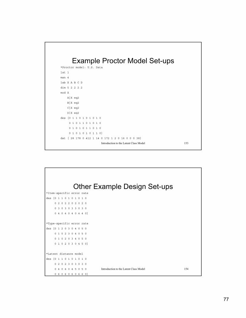
Example Proctor Model Set-ups*Proctor model: U.S. Data
lat 1
man 4man 4
lab X A B C D
dim 5 2 2 2 2
mod X
A|X eq2
B|X eq2
C|X eq2
D|X eq2
Introduction to the Latent Class Model 153
| q
des [0 1 1 0 1 0 1 0 1 0
0 1 0 1 1 0 1 0 1 0
0 1 0 1 0 1 1 0 1 0
0 1 0 1 0 1 0 1 1 0]
dat [ 28 178 0 412 1 14 0 172 1 2 0 16 0 0 0 38]
Other Example Design Set-ups*Item-specific error rate
des [0 1 1 0 1 0 1 0 1 0
0 2 0 2 2 0 2 0 2 00 2 0 2 2 0 2 0 2 0
0 3 0 3 0 3 3 0 3 0
0 4 0 4 0 4 0 4 4 0]
*Type-specific error rate
des [0 1 2 0 3 0 4 0 5 0
0 1 0 2 3 0 4 0 5 0
0 1 0 2 0 3 4 0 5 0
Introduction to the Latent Class Model 154
0 1 0 2 0 3 0 4 5 0]
*Latent distance model
des [0 1 1 0 1 0 1 0 1 0
0 2 0 2 3 0 3 0 3 0
0 4 0 4 0 4 5 0 5 0
0 6 0 6 0 6 0 6 6 0]
78
Simultaneous Latent Class Models
Simultaneous LCMs
• Basic latent class model• Basic latent class model
• Let Gs represent external (i.e., non-indicator) grouping variable
XDlt
XCkt
XBjt
XAit
Xt
ABCDXijklt
||||
Introduction to the Latent Class Model 156
indicator) grouping variable
• Simultaneous latent class modelGs
XGDlts
XGCkts
XGBjts
XGAits
GXts
ABCDXGijklts |||||
79
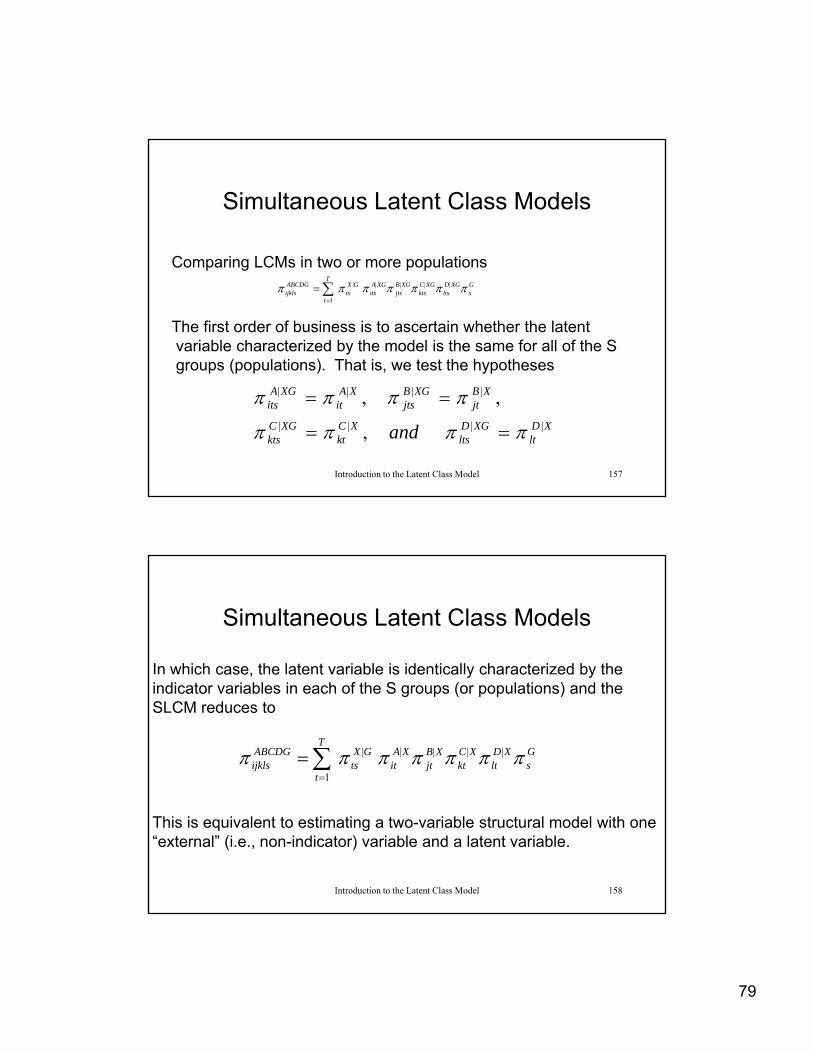
Simultaneous Latent Class Models
C i LCM i t l tiComparing LCMs in two or more populations
The first order of business is to ascertain whether the latentvariable characterized by the model is the same for all of the Sgroups (populations). That is, we test the hypotheses
Gs
XGDlts
XGCkts
XGBjts
XGAits
T
t
GXts
ABCDGijkls ||||
1
|
Introduction to the Latent Class Model 157
XDlt
XGDlts
XCkt
XGCkts
XBjt
XGBjts
XAit
XGAits
and ||||
||||
,
,,
Simultaneous Latent Class Models
In which case, the latent variable is identically characterized by the c case, t e ate t a ab e s de t ca y c a acte ed by t eindicator variables in each of the S groups (or populations) and the SLCM reduces to
Gs
XDlt
XCkt
XBjt
XAit
T
t
GXts
ABCDGijkls ||||
1
|
Introduction to the Latent Class Model 158
This is equivalent to estimating a two-variable structural model with one “external” (i.e., non-indicator) variable and a latent variable.
80
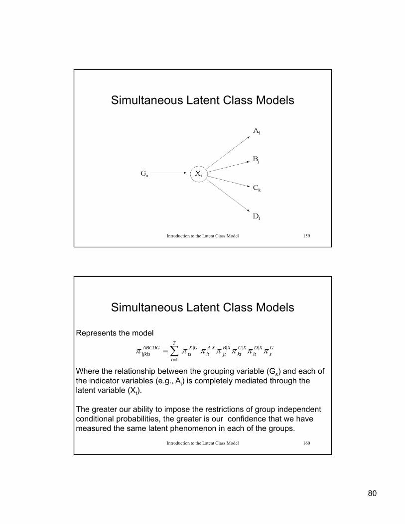
Simultaneous Latent Class Models
Introduction to the Latent Class Model 159
Simultaneous Latent Class Models
Represents the modelep ese ts t e ode
Where the relationship between the grouping variable (Gs) and each of the indicator variables (e.g., Ai) is completely mediated through the latent variable (Xt).
Gs
XDlt
XCkt
XBjt
XAit
T
t
GXts
ABCDGijkls ||||
1
|
Introduction to the Latent Class Model 160
The greater our ability to impose the restrictions of group independent conditional probabilities, the greater is our confidence that we have measured the same latent phenomenon in each of the groups.
81
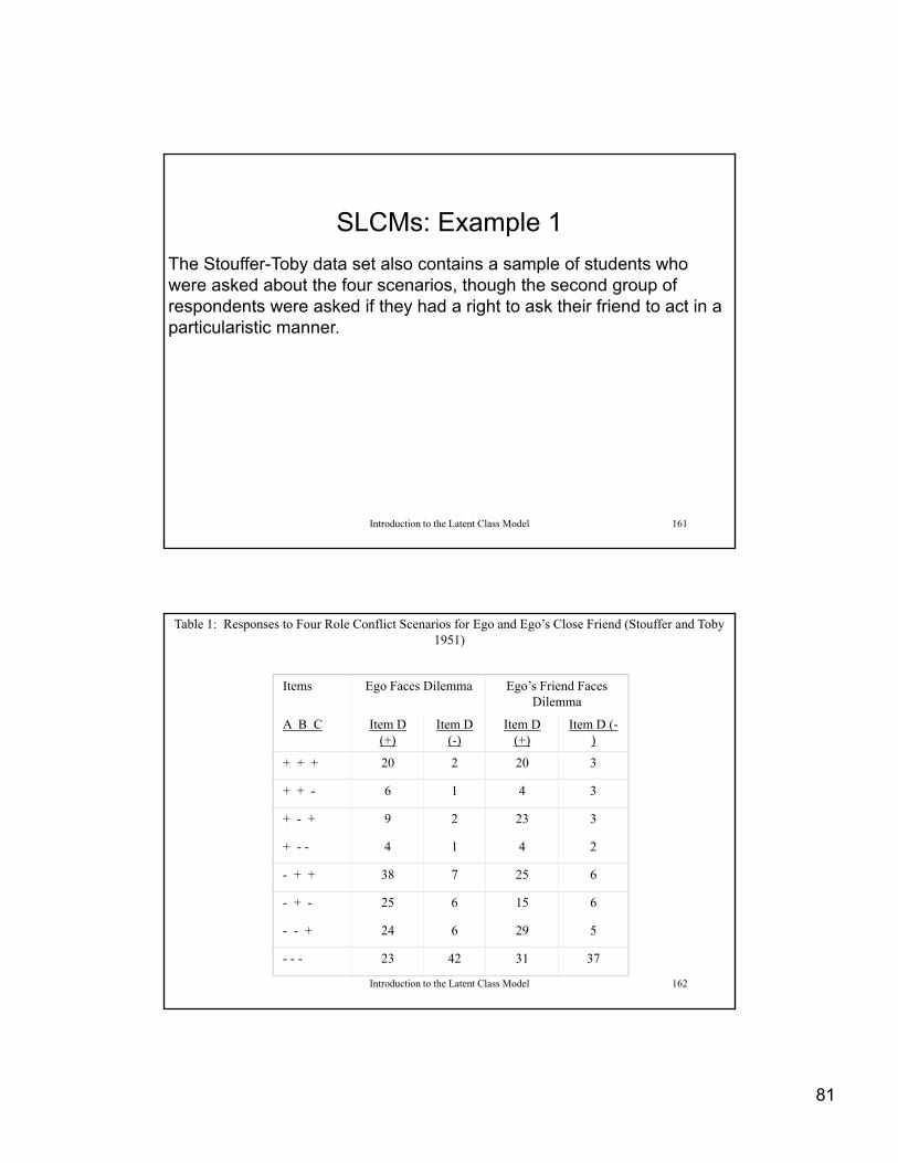
SLCMs: Example 1
The Stouffer-Toby data set also contains a sample of students who were asked about the four scenarios though the second group ofwere asked about the four scenarios, though the second group of respondents were asked if they had a right to ask their friend to act in a particularistic manner.
Introduction to the Latent Class Model 161
Table 1: Responses to Four Role Conflict Scenarios for Ego and Ego’s Close Friend (Stouffer and Toby 1951)
Items Ego Faces Dilemma Ego’s Friend Faces Dilemma
A B C Item D (+)
Item D (-)
Item D (+)
Item D (-)( ) ( ) ( ) )
+ + + 20 2 20 3
+ + - 6 1 4 3
+ - + 9 2 23 3
+ - - 4 1 4 2
- + + 38 7 25 6
Introduction to the Latent Class Model 162
+ + 38 7 25 6
- + - 25 6 15 6
- - + 24 6 29 5
- - - 23 42 31 37

82
Table 2: Simultaneous Latent Class Model Evaluation Criteria for Universalism Data
Model X2 G2 AIC BIC DF
H1: Unrestricted 2-Class / group Model
9.06 8.25 -15.75 -64.57 12
H2: Structural Homogeneity
24.78 23.47 -16.53 -97.90 20
H : Complete 24 82 23 48 -18 52 -103 96 21
Introduction to the Latent Class Model 163
H3: Complete Homogeneity
24.82 23.48 -18.52 -103.96 21
Table 3: Simultaneous Latent Class Parameters, Complete Homogeneity Two-Class Model: Stouffer-Toby Data
==============================================================Observed Respondent TypeObserved Respondent Type
Variables Universalistic Particularistic————————————————————————————————Auto Passenger Friend .990 .655Drama Critic Friend .892 .433Insurance Doctor Friend .979 .283Board of Directors Friend .681 .151————————————————————————————————
Latent Class Probabilities .2917 .7083
Introduction to the Latent Class Model 164
————————————————————————————————————

83
LEM
* SLCM, Complete Homogeneity, Stouffer-* Toby Datalat 1man 5 dim 2 2 2 2 2 2lab X G A B C Dmod X|G eq2
A|X B|X C|X D|X
des [1 1 0 0]d [20 2 6 1 9 2 4 1 38 7 25 6 24 6 23 42
Introduction to the Latent Class Model 165
dat [20 2 6 1 9 2 4 1 38 7 25 6 24 6 23 4220 3 4 3 23 3 4 2 25 6 15 6 29 5 31 37]
Belief in God (Measurement Error): 1991 ISSP
Q.14 Please tick one box below to show which statement comes closest toexpressing what you believe about God. (Please tick one box only)-------------------------------------------------------------
1. I don't believe in God 1. I don t believe in God2. I don't know whether there is a God and I don't believe there is any
way to find out3. I don't believe in a personal God, but I do believe in a Higher Power of
some kind 4. I find myself believing in God some of the time, but not at others 5. While I have doubts, I feel that I do believe in God 6. I know God really exists and I have no doubts about it 8. Can't choose, don't know
Q.15 How close do you feel to God most of the time?(Please tick one box only)
Introduction to the Latent Class Model 166
( y)-------------------------------------------------------------- 1. Don't believe in God 2. Not close at all 3. Not very close 4. Somewhat close 5. Extremely close 8. Can't choose, don't know
9. NA, refused

84
Belief in God (Measurement Error): 1991 ISSP
Q.16 Which best describes your beliefs about God?(Please tick one box only)
-------------------------------------------------- 1. I don't believe in God now and I never have 2. I don't believe in God now, but I used to 3. I believe in God now, but I didn't used to 4. I believe in God now and I always have 8. Can't choose, don't know
9. NA, refused
Introduction to the Latent Class Model 167
Example 2: Belief in God (Germany, 1991 ISSP Data)
* 1991 ISSP Belief in God data: a=v33, * b=v32, c=v31, L=lander; dichotomized with * 1=don't, 2= believinglat 1man 4 dim 2 2 2 2 2lab X L A B C mod X|L
A|XL eq2B|XC|XL eq2
Introduction to the Latent Class Model 168
C|XL eq2des [0 0 0 0 1 0 1 0
0 2 0 2 0 0 0 0]sta A|XL [.5 .5 .5 .5 .9 .1 .9 .1]dat [107 31 8 276 4 1 18 901
674 82 37 306 5 4 7 371]

85
Table 7: Simultaneous Latent Class Parameters, Restricted Belief in God Data: ISSP 1991, West & East Germany
========================================================Observed West EastObserved West East
Variables Believe Not Believe Not————————————————————————————————Express .767 .013* .551 .013*Close .998* .043* .998* .043*Describe .982* .218 .982* .110————————————————————————————————LC Probs. .8909 .1091 .4629 .5371————————————————————————————————
Introduction to the Latent Class Model 169
*1991 ISSP Belief in God data: a=v33, * b=v32, c=v31, L=lander dichotomized* with 1=don't believe, 2= believingl 1lat 1man 4 dim 2 2 2 2 2lab X L A B C mod X|L
A|XL AX,ALB|XC|XL CX,CL
dat [107 31 8 276 4 1 18 901 674 82 37 306 5 4 7 371]
Introduction to the Latent Class Model 170
674 82 37 306 5 4 7 371]

86
Log-linear models with latent variables (latent logistic “mimic” model)
Introduction to the Latent Class Model 171
Probabilistic parameterization (“saturated model”)
EFGops
XEFGDltops
XEFGCktops
XEFGBjtops
XEFGAitops
T
t
EFGXtops
ABCDEFGijklops ||||
1
|
T
Probabilistic parameterization ( saturated model )
“Reduced” Model (above)
Introduction to the Latent Class Model 172
Gs
Fp
Eo
XDlt
XCkt
XBjt
XAit
T
t
GXts
FXtp
EXto
ABCDEFGijklops ||||
1
|||

87
Log-linear Parameterization
EFGops
EFop
XEFGtops
XEFtop
DXEFGltops
AXEFGitops
DXFGltps
AXEFitop
DXGlts
AXEito
DGls
CGks
DElo
CEko
BEjo
AEio
XGts
XFtp
XEto
DXlt
CXkt
BXjt
AXit
Dl
Ck
Bj
Ai
Xt
Gs
Fp
Eo
ABCDXEFG
ijkltopsF
)ln(^
Introduction to the Latent Class Model 173
opsoptopstopltops
DGCGBGAGXGXFXEDXCXBXAX
Dl
Ck
Bj
Ai
Xt
Gs
Fp
Eo
ABCDXEFG
ijkltopsF
)ln(^
Reduced
DGls
CGks
BGjs
AGis
XGts
XFtp
XEto
DXlt
CXkt
BXjt
AXit
Logit
)ln()ln(ln 2
^
1
^
^1
^ ABCDXEFG
opsijkl
ABCDXEFG
opsijklABCDXEFG
ABCDXEFG
opsijkl FFF
Introduction to the Latent Class Model 174
)()(2opsijklF
88
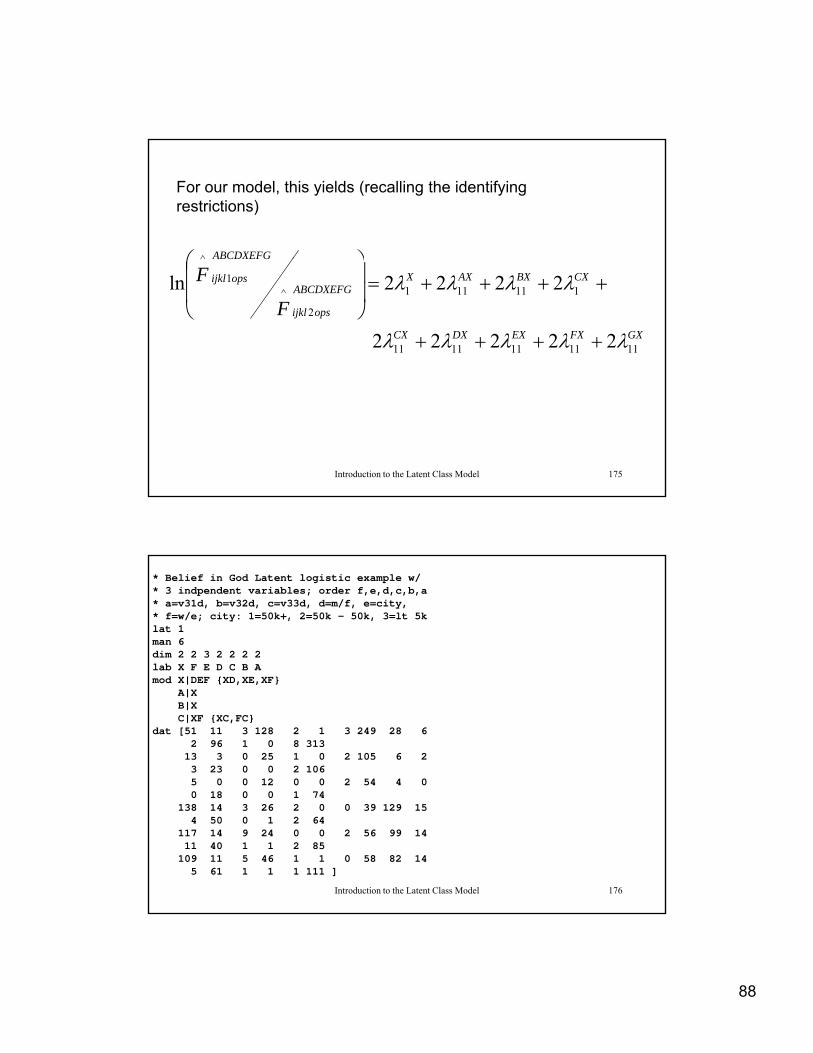
For our model, this yields (recalling the identifying restrictions)
ABCDXEFG^
GXFXEXDXCX
CXBXAXXABCDXEFG
opsijkl
ABCDXEFG
opsijkl
F
F
1111111111
111111
2
^1
^
22222
2222ln
Introduction to the Latent Class Model 175
* Belief in God Latent logistic example w/ * 3 indpendent variables; order f,e,d,c,b,a* a=v31d, b=v32d, c=v33d, d=m/f, e=city, * f=w/e; city: 1=50k+, 2=50k - 50k, 3=lt 5klat 1man 6dim 2 2 3 2 2 2 2lab X F E D C B Amod X|DEF XD,XE,XF
A|XB|XC|XF XC,FC
dat [51 11 3 128 2 1 3 249 28 6 2 96 1 0 8 313
13 3 0 25 1 0 2 105 6 2 3 23 0 0 2 1065 0 0 12 0 0 2 54 4 0 0 18 0 0 1 74
Introduction to the Latent Class Model 176
0 18 0 0 1 74138 14 3 26 2 0 0 39 129 15
4 50 0 1 2 64117 14 9 24 0 0 2 56 99 14 11 40 1 1 2 85
109 11 5 46 1 1 0 58 82 14 5 61 1 1 1 111 ]
89
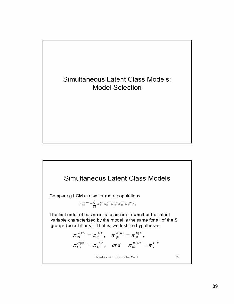
Simultaneous Latent Class Models: Model Selection
Simultaneous Latent Class Models
C i LCM i t l tiComparing LCMs in two or more populations
The first order of business is to ascertain whether the latentvariable characterized by the model is the same for all of the Sgroups (populations). That is, we test the hypotheses
Gs
XGDlts
XGCkts
XGBjts
XGAits
T
t
GXts
ABCDGijkls ||||
1
|
Introduction to the Latent Class Model 178
XDlt
XGDlts
XCkt
XGCkts
XBjt
XGBjts
XAit
XGAits
and ||||
||||
,
,,
90
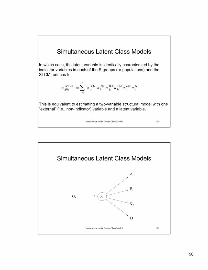
Simultaneous Latent Class Models
In which case, the latent variable is identically characterized by the c case, t e ate t a ab e s de t ca y c a acte ed by t eindicator variables in each of the S groups (or populations) and the SLCM reduces to
Gs
XDlt
XCkt
XBjt
XAit
T
t
GXts
ABCDGijkls ||||
1
|
Introduction to the Latent Class Model 179
This is equivalent to estimating a two-variable structural model with one “external” (i.e., non-indicator) variable and a latent variable.
Simultaneous Latent Class Models
Introduction to the Latent Class Model 180

91
Simultaneous Latent Class Models
Represents the modelep ese ts t e ode
Where the relationship between the grouping variable (Gs) and each of the indicator variables (e.g., Ai) is completely mediated through the latent variable (Xt).
Gs
XDlt
XCkt
XBjt
XAit
T
t
GXts
ABCDGijkls ||||
1
|
Introduction to the Latent Class Model 181
The greater our ability to impose the restrictions of group independent conditional probabilities, the greater is our confidence that we have measured the same latent phenomenon in each of the groups.
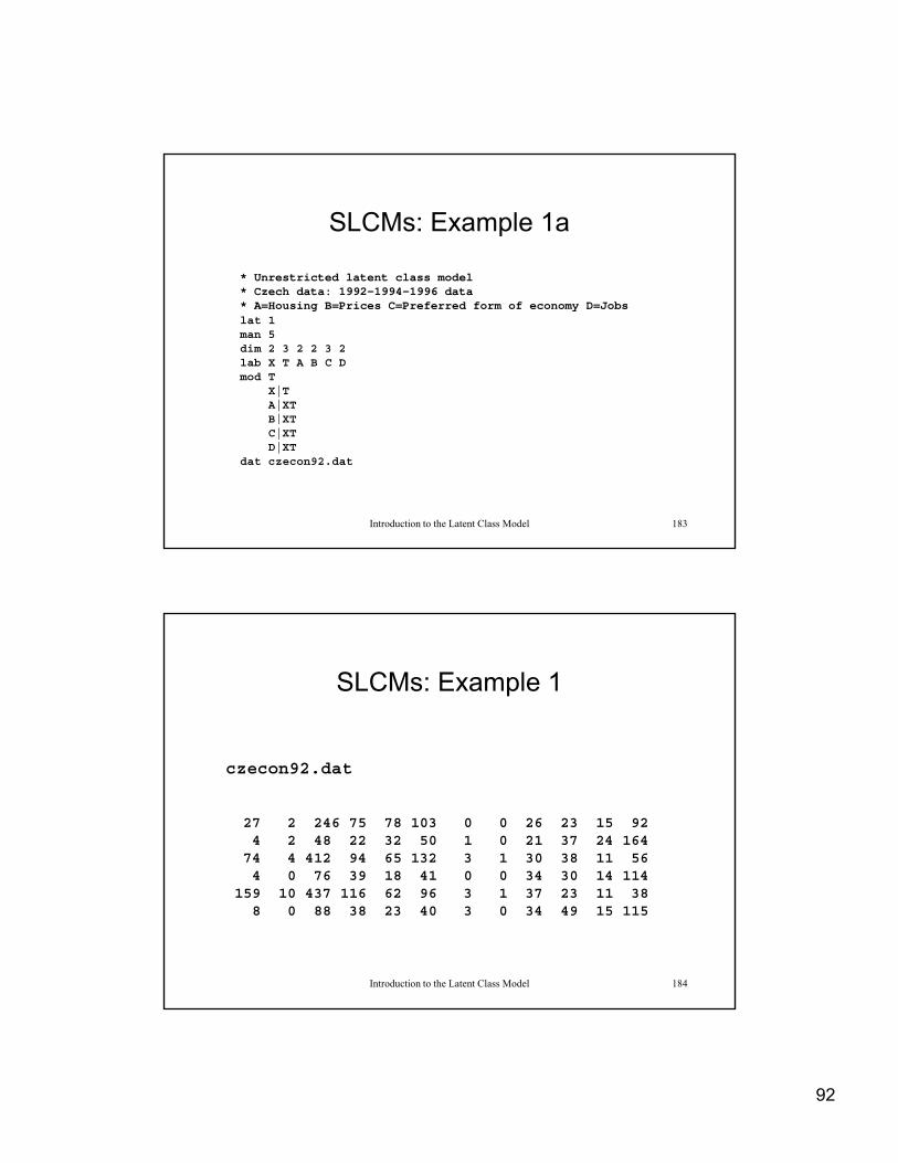
SLCMs: Example 11992-1994-1996 Czech Republic (Economic Expectations data)
Do you generally prefer an economy:
1 as socialist, which was in our country before 1989
2 as a social market with a high degree of state intervention
3 as a free market with minimal state intervention?”
According to you should the state administratively fix prices more?
Introduction to the Latent Class Model 182
According to you, should the state administratively fix prices more?
Should the state provide a job for everyone who wants to work?
Do you think that the state should provide housing for every family which is not able to find it?
92
SLCMs: Example 1a
* Unrestricted latent class model* Czech data: 1992-1994-1996 data* A=Housing B=Prices C=Preferred form of economy D=Jobslat 1man 5dim 2 3 2 2 3 2lab X T A B C Dmod T
X|TA|XTB|XT
Introduction to the Latent Class Model 183
B|XTC|XTD|XT
dat czecon92.dat
SLCMs: Example 1
czecon92.dat
27 2 246 75 78 103 0 0 26 23 15 924 2 48 22 32 50 1 0 21 37 24 16474 4 412 94 65 132 3 1 30 38 11 56 4 0 76 39 18 41 0 0 34 30 14 114
Introduction to the Latent Class Model 184
4 0 76 39 18 41 0 0 34 30 14 114159 10 437 116 62 96 3 1 37 23 11 38 8 0 88 38 23 40 3 0 34 49 15 115
93
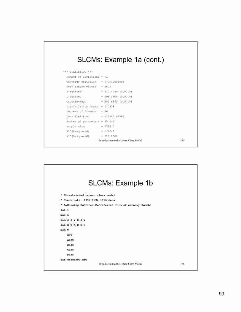
SLCMs: Example 1a (cont.)
*** STATISTICS ***
Number of iterations = 72Number of iterations = 72
Converge criterion = 0.0000008801
Seed random values = 3602
X-squared = 310.4235 (0.0000)
L-squared = 298.0800 (0.0000)
Cressie-Read = 302.8963 (0.0000)
Dissimilarity index = 0.0938
Degrees of freedom = 36
Introduction to the Latent Class Model 185
Degrees of freedom 36
Log-likelihood = -13586.64568
Number of parameters = 35 (+1)
Sample size = 3788.0
BIC(L-squared) = 1.4547
AIC(L-squared) = 226.0800
SLCMs: Example 1b
* Unrestricted latent class model
* Czech data: 1992 1994 1996 data* Czech data: 1992-1994-1996 data
* A=Housing B=Prices C=Preferred form of economy D=Jobs
lat 1
man 5
dim 3 3 2 2 3 2
lab X T A B C D
mod T
X|T
Introduction to the Latent Class Model 186
X|T
A|XT
B|XT
C|XT
D|XT
dat czecon92.dat
94
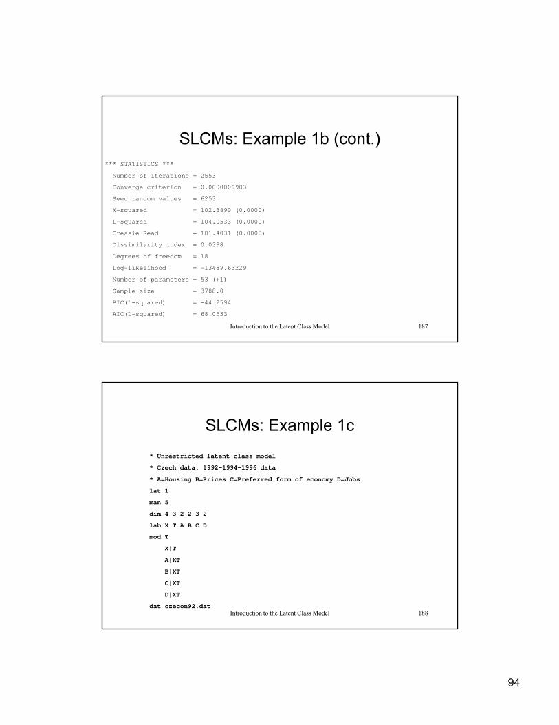
SLCMs: Example 1b (cont.)*** STATISTICS ***
Number of iterations = 2553
Converge criterion = 0.0000009983
Seed random values = 6253
X-squared = 102.3890 (0.0000)
L-squared = 104.0533 (0.0000)
Cressie-Read = 101.4031 (0.0000)
Dissimilarity index = 0.0398
Degrees of freedom = 18
Introduction to the Latent Class Model 187
Log-likelihood = -13489.63229
Number of parameters = 53 (+1)
Sample size = 3788.0
BIC(L-squared) = -44.2594
AIC(L-squared) = 68.0533
SLCMs: Example 1c
* Unrestricted latent class model
* Czech data: 1992-1994-1996 data
* A=Housing B=Prices C=Preferred form of economy D=Jobs
lat 1
man 5
dim 4 3 2 2 3 2
lab X T A B C D
mod T
X|T
Introduction to the Latent Class Model 188
X|T
A|XT
B|XT
C|XT
D|XT
dat czecon92.dat
95
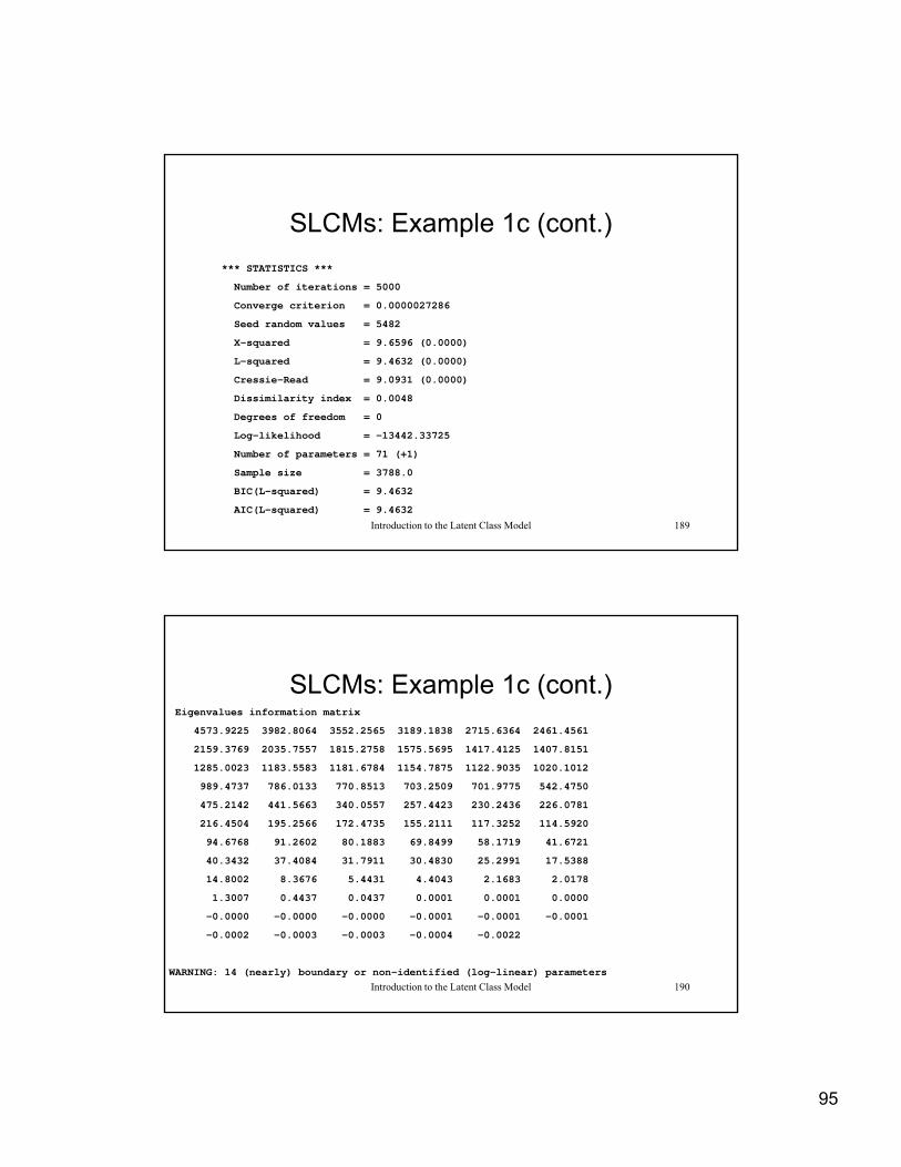
SLCMs: Example 1c (cont.)
*** STATISTICS ***
Number of iterations = 5000Number of iterations = 5000
Converge criterion = 0.0000027286
Seed random values = 5482
X-squared = 9.6596 (0.0000)
L-squared = 9.4632 (0.0000)
Cressie-Read = 9.0931 (0.0000)
Dissimilarity index = 0.0048
Degrees of freedom = 0
Introduction to the Latent Class Model 189
Degrees of freedom 0
Log-likelihood = -13442.33725
Number of parameters = 71 (+1)
Sample size = 3788.0
BIC(L-squared) = 9.4632
AIC(L-squared) = 9.4632
SLCMs: Example 1c (cont.)Eigenvalues information matrix
4573.9225 3982.8064 3552.2565 3189.1838 2715.6364 2461.4561
2159 3769 2035 7557 1815 2758 1575 5695 1417 4125 1407 81512159.3769 2035.7557 1815.2758 1575.5695 1417.4125 1407.8151
1285.0023 1183.5583 1181.6784 1154.7875 1122.9035 1020.1012
989.4737 786.0133 770.8513 703.2509 701.9775 542.4750
475.2142 441.5663 340.0557 257.4423 230.2436 226.0781
216.4504 195.2566 172.4735 155.2111 117.3252 114.5920
94.6768 91.2602 80.1883 69.8499 58.1719 41.6721
40.3432 37.4084 31.7911 30.4830 25.2991 17.5388
14 8002 8 3676 5 4431 4 4043 2 1683 2 0178
Introduction to the Latent Class Model 190
14.8002 8.3676 5.4431 4.4043 2.1683 2.0178
1.3007 0.4437 0.0437 0.0001 0.0001 0.0000
-0.0000 -0.0000 -0.0000 -0.0001 -0.0001 -0.0001
-0.0002 -0.0003 -0.0003 -0.0004 -0.0022
WARNING: 14 (nearly) boundary or non-identified (log-linear) parameters

96
SLCMs: Example 1(cont.)* Restricted latent class model* Czech data: 1992-1994-1996 data* A=Housing B=Prices C=Preferred form of economy D=Jobs*lat 1man 5dim 4 3 2 2 3 2lab X T A B C Dmod T
X|TA|XTB|XTC|XT
D|XTsta A|XT [0 1 0 1 0 1 .5 .5 .5 .5 .5 .5
.6 .4 .6 .4 .6 .4 .4 .6 .4 .6 .4 .6 ]sta B|XT [0 1 0 1 0 1 .5 .5 .5 .5 .5 .5
6 4 6 4 6 4 4 6 4 6 4 6 ]
Introduction to the Latent Class Model 191
.6 .4 .6 .4 .6 .4 .4 .6 .4 .6 .4 .6 ]sta C|XT [0 .5 .5 0 .5 .5 0 .5 .5 .33 .33 .34 .33 .33 .34 .33 .33
.34 0 .5 .5 0 .5 .5 0 .5 .5 0 .5 .5 0 .5 .5 0 .5 .5 ]sta D|XT [0 1 0 1 0 1 .5 .5 .5 .5 .5 .5
.6 .4 .6 .4 .6 .4 .4 .6 .4 .6 .4 .6 ]dat czecon92.dat
*** STATISTICS ***
Number of iterations = 2886
Converge criterion = 0.0000009992
Seed random values = 6220
38 93 0 0 0000X-squared = 38.9340 (0.0000)
L-squared = 28.9340 (0.0000)
Cressie-Read = 33.3781 (0.0000)
Dissimilarity index = 0.0133
Degrees of freedom = 0
Log-likelihood = -13452.07266
Introduction to the Latent Class Model 192
Number of parameters = 71 (+1)
Sample size = 3788.0
BIC(L-squared) = 28.9340
AIC(L-squared) = 28.9340

97
SLCMs: Example 1(cont.)* Restricted latent class model* Czech data: 1992-1994-1996 data* A=Housing B=Prices C=Preferred form of economy D=Jobs*lat 1man 5dim 4 3 2 2 3 2lab X T A B C Dmod T
X|TA|XT eq2B|XT eq2C|XT eq2
D|XT eq2des [0 -1 0 -1 0 –1 0 0 0 0 0 0 0 0 0 0 0 0 0 0 0 0 0 0
0 -1 0 -1 0 –1 0 0 0 0 0 0 0 0 0 0 0 0 0 0 0 0 0 0-1 0 0 –1 0 0 -1 0 0 0 0 0 0 0 0 0 0 01 0 0 1 0 0 1 0 0 1 0 0 1 0 0 1 0 0
Introduction to the Latent Class Model 193
-1 0 0 -1 0 0 -1 0 0 -1 0 0 -1 0 0 -1 0 0 0 -1 0 -1 0 -1 0 0 0 0 0 0 0 0 0 0 0 0 0 0 0 0 0 0 0]
sta A|XT [0 1 0 1 0 1 .5 .5 .5 .5 .5 .5 .6 .4 .6 .4 .6 .4 .4 .6 .4 .6 .4 .6 ]
sta B|XT [0 1 0 1 0 1 .5 .5 .5 .5 .5 .5 .6 .4 .6 .4 .6 .4 .4 .6 .4 .6 .4 .6 ]
sta C|XT [0 .5 .5 0 .5 .5 0 .5 .5 .33 .33 .34 .33 .33 .34 .33 .33 .34 0 .5 .5 0 .5 .5 0 .5 .5 0 .5 .5 0 .5 .5 0 .5 .5 ]
sta D|XT [0 1 0 1 0 1 .5 .5 .5 .5 .5 .5 .6 .4 .6 .4 .6 .4 .4 .6 .4 .6 .4 .6 ]
dat czecon92.dat
*** STATISTICS ***
Number of iterations = 2929
Converge criterion = 0.0000009999
Seed random values = 3199
X-squared = 38.9330 (0.0029)
L-squared = 28.9340 (0.0492)
Cressie-Read = 33.3776 (0.0150)
Dissimilarity index = 0.0133
Degrees of freedom = 18
Log-likelihood = -13452.07267
Number of parameters = 53 (+1)
Sample size = 3788 0
Introduction to the Latent Class Model 194
Sample size = 3788.0
BIC(L-squared) = -119.3787
AIC(L-squared) = -7.0660
WARNING: no information is provided on identification of parameters

98
SLCMs: Example 1(cont.)* Restricted latent class model* Czech data: 1992-1994-1996 data* A=Housing B=Prices C=Preferred form of economy D=Jobs*lat 1man 5dim 4 3 2 2 3 2lab X T A B C Dmod T
X|TA|XT eq2B|XT eq2C|XT eq2
D|XT eq2des [0 -1 0 -1 0 –1 0 1 0 1 0 1 0 2 0 2 0 2 0 3 0 3 0 3 0
0 -1 0 -1 0 -1 0 4 0 4 0 4 0 5 0 5 0 5 0 6 0 6 0 6 0-1 0 0 –1 0 0 -1 0 0 0 0 0 0 0 0 0 0 0 1 0 0 1 0 0 1 0 0 1 0 0 1 0 0 1 0 0
Introduction to the Latent Class Model 195
-1 0 0 -1 0 0 -1 0 0 -1 0 0 -1 0 0 -1 0 0 0 -1 0 -1 0 -1 0 7 0 7 0 7 0 8 0 8 0 8 0 9 0 9 0 9 0]
sta A|XT [0 1 0 1 0 1 .5 .5 .5 .5 .5 .5 .6 .4 .6 .4 .6 .4 .4 .6 .4 .6 .4 .6 ]
sta B|XT [0 1 0 1 0 1 .5 .5 .5 .5 .5 .5 .6 .4 .6 .4 .6 .4 .4 .6 .4 .6 .4 .6 ]
sta C|XT [0 .5 .5 0 .5 .5 0 .5 .5 .33 .33 .34 .33 .33 .34 .33 .33 .34 0 .5 .5 0 .5 .5 0 .5 .5 0 .5 .5 0 .5 .5 0 .5 .5 ]
sta D|XT [0 1 0 1 0 1 .5 .5 .5 .5 .5 .5 .6 .4 .6 .4 .6 .4 .4 .6 .4 .6 .4 .6 ]
dat czecon92.dat
*** STATISTICS ***
Number of iterations = 299
Converge criterion = 0.0000009841
Seed random values = 132
X-squared = 79.3459 (0.0000)
L-squared = 62.2769 (0.0042)
Cressie-Read = 70.1651 (0.0006)
Dissimilarity index = 0.0312
Degrees of freedom = 36
Log-likelihood = -13468 74411
Introduction to the Latent Class Model 196
Log-likelihood = -13468.74411
Number of parameters = 35 (+1)
Sample size = 3788.0
BIC(L-squared) = -234.3485
AIC(L-squared) = -9.7231

99
Table 1: Conditional Response Probabilities for Modeled Trend Data: Czech Preferred Form of Economy
ClassIndicator 1 2 3 4
1992Economy
Socialist .00* .09 .00* .00*Social Market .14 .73 .50 .26Free Market .86 .18 .50 .74
Housing .00* .92* .33* .25*Prices 00* 97* 57* 66*Prices .00 .97 .57 .66Jobs .00* .91* .74* .05*
1994Economy
Socialist .00* .14 .00* .00*Social Market .09 .76 .75 .33Free Market .91 .10 .25 .67
Housing .00* .92* .33* .25*Prices .00* .97* .57* .66*Jobs .00* .91* .74* .05*
1996
Introduction to the Latent Class Model 197
1996Economy
Socialist .00* .24 .00* .00*Social Market .22 .68 .72 .38Free Market .78 .08 .28 .62
Housing .00* .92* .33* .25*Prices .00* .97* .57* .66*Jobs .00* .91* .74* .05*
Table 1: Latent Class Probabilities for Modeled Trend Data: Czech Preferred Form of Economy
ClassYear 1 2 3 4
1992 .145 .362 .178 .3161994 .076 .485 .154 .2851996 .087 .543 .162 .208
Introduction to the Latent Class Model 198

100
Belief in God (Measurement Error): 1991 ISSP
Q.14 Please tick one box below to show which statement comes closest toexpressing what you believe about God. (Please tick one box only)-------------------------------------------------------------
1. I don't believe in God 1. I don t believe in God2. I don't know whether there is a God and I don't believe there is any
way to find out3. I don't believe in a personal God, but I do believe in a Higher Power of
some kind 4. I find myself believing in God some of the time, but not at others 5. While I have doubts, I feel that I do believe in God 6. I know God really exists and I have no doubts about it 8. Can't choose, don't know
Q.15 How close do you feel to God most of the time?(Please tick one box only)
Introduction to the Latent Class Model 199
( y)-------------------------------------------------------------- 1. Don't believe in God 2. Not close at all 3. Not very close 4. Somewhat close 5. Extremely close 8. Can't choose, don't know
9. NA, refused
Belief in God (Measurement Error): 1991 ISSP
Q.16 Which best describes your beliefs about God?(Please tick one box only)
-------------------------------------------------- 1. I don't believe in God now and I never have 2. I don't believe in God now, but I used to 3. I believe in God now, but I didn't used to 4. I believe in God now and I always have 8. Can't choose, don't know
9. NA, refused
Introduction to the Latent Class Model 200

101
Example 2: Belief in God (Germany, 1991 ISSP Data)
* 1991 ISSP Belief in God data: a=v33, * b=v32, c=v31, L=lander; dichotomized with * 1=don't, 2= believinglat 1man 4 dim 2 2 2 2 2lab X L A B C mod X|L
A|XL eq2B|XC|XL eq2
des [0 0 0 0 1 0 1 0
Introduction to the Latent Class Model 201
des [0 0 0 0 1 0 1 00 2 0 2 0 0 0 0]
sta A|XL [.5 .5 .5 .5 .9 .1 .9 .1]dat [107 31 8 276 4 1 18 901
674 82 37 306 5 4 7 371]
Table 7: Simultaneous Latent Class Parameters, Restricted Belief in God Data: ISSP 1991, West & East Germany
========================================================Observed West EastObserved West East
Variables Believe Not Believe Not————————————————————————————————Express .767 .013* .551 .013*Close .998* .043* .998* .043*Describe .982* .218 .982* .110————————————————————————————————LC Probs. .8909 .1091 .4629 .5371————————————————————————————————
Introduction to the Latent Class Model 202
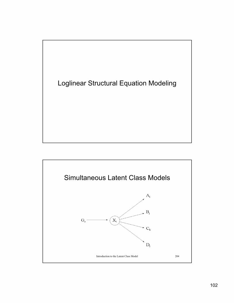
102
Loglinear Structural Equation Modeling
Simultaneous Latent Class Models
Introduction to the Latent Class Model 204

103
Simultaneous Latent Class Models
Represents the modelep ese ts t e ode
Where the relationship between the grouping variable (Gs) and each of the indicator variables (e.g., Ai) is completely mediated through the latent variable (Xt).
Gs
XDlt
XCkt
XBjt
XAit
T
t
GXts
ABCDGijkls ||||
1
|
Introduction to the Latent Class Model 205
The greater our ability to impose the restrictions of group independent conditional probabilities, the greater is our confidence that we have measured the same latent phenomenon in each of the groups.
Belief in God (Measurement Error): 1991 ISSP
Q.14 Please tick one box below to show which statement comes closest toexpressing what you believe about God. (Please tick one box only)-------------------------------------------------------------
1. I don't believe in God 1. I don t believe in God2. I don't know whether there is a God and I don't believe there is any
way to find out3. I don't believe in a personal God, but I do believe in a Higher Power of
some kind 4. I find myself believing in God some of the time, but not at others 5. While I have doubts, I feel that I do believe in God 6. I know God really exists and I have no doubts about it 8. Can't choose, don't know
Q.15 How close do you feel to God most of the time?(Please tick one box only)
Introduction to the Latent Class Model 206
( y)-------------------------------------------------------------- 1. Don't believe in God 2. Not close at all 3. Not very close 4. Somewhat close 5. Extremely close 8. Can't choose, don't know
9. NA, refused
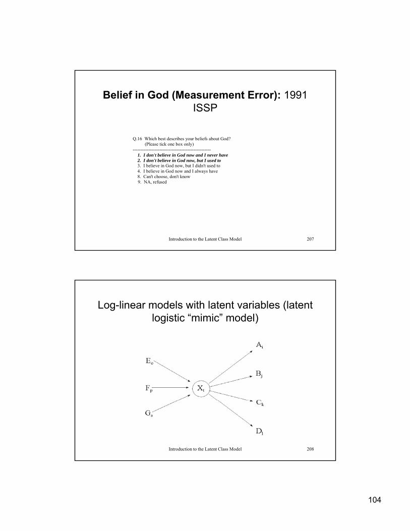
104
Belief in God (Measurement Error): 1991 ISSP
Q.16 Which best describes your beliefs about God?(Please tick one box only)
-------------------------------------------------- 1. I don't believe in God now and I never have 2. I don't believe in God now, but I used to 3. I believe in God now, but I didn't used to 4. I believe in God now and I always have 8. Can't choose, don't know
9. NA, refused
Introduction to the Latent Class Model 207
Log-linear models with latent variables (latent logistic “mimic” model)
Introduction to the Latent Class Model 208
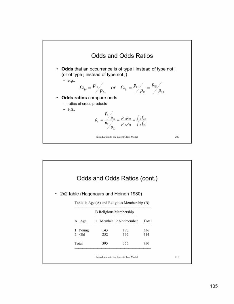
105
Odds and Odds Ratios
• Odds that an occurrence is of type i instead of type not i (or of type j instead of type not j)(or of type j instead of type not j) – e.g.,
• Odds ratios compare odds– ratios of cross products
e g
1|2
1|1
12
111|1
2
11 p
pp
porpp
Introduction to the Latent Class Model 209
– e.g.,
2112
2211
2112
2211
22
21
12
11
11 ff
ff
pp
pp
pp
pp
Odds and Odds Ratios (cont.)
• 2x2 table (Hagenaars and Heinen 1980)2x2 table (Hagenaars and Heinen 1980)
Table 1: Age (A) and Religious Membership (B)
B. Religious Membership
A. Age 1. Member 2.Nonmember Total1 Y 143 193 336
Introduction to the Latent Class Model 210
1. Young 143 193 3362. Old 252 162 414
Total 395 355 750

106
Odds and Odds Ratios (cont.)
• Marginal odds: e g Ω1+ = 336/414 = 812Marginal odds: e.g., Ω1+ 336/414 .812
– odds of subject being young relative to being old in this table
• Conditional odds: e.g. Ω1|1 = 143/193 = .741
– Young people are (1/.741=) 1.35 times more likely to
Introduction to the Latent Class Model 211
be nonmember than member
Odds and Odds Ratios (cont.)
• Odds ratio: θ11 = (143/193)/(252/162) =Odds ratio: θ11 (143/193)/(252/162) (143x162)/(252x193) = .476 (approx. .5)
– the odds of a younger person being a member of a denomination is only half those of an older person
– among members, the odds of being an older person is about twice that of being a younger person
Odd ti i d d t f th i l di t ib ti
Introduction to the Latent Class Model 212
• Odds ratios are independent of the marginal distributions of variables
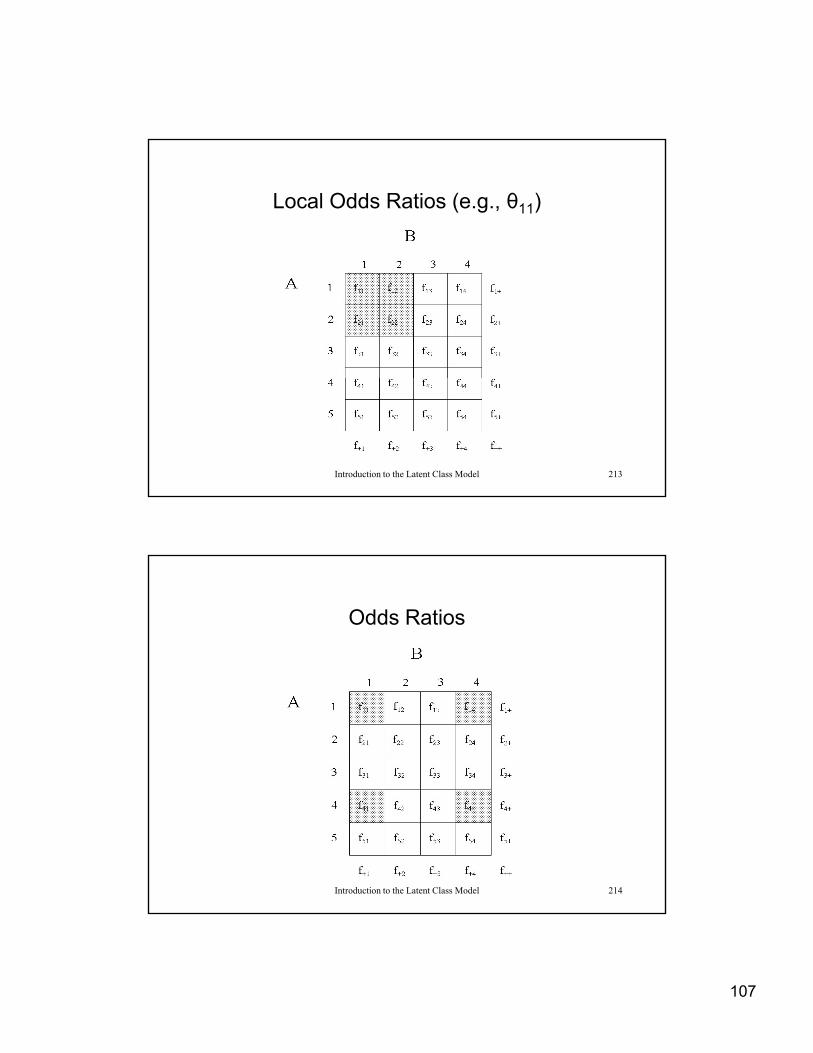
107
Local Odds Ratios (e.g., θ11)
Introduction to the Latent Class Model 213
Odds Ratios
Introduction to the Latent Class Model 214

108
Geometric Averages
• Multiplicative modelsMultiplicative models
• Partial odds ratio
nn
nn
iigeom XXXXX 21
1
Introduction to the Latent Class Model 215
KK
KK
kkp 11112111
1
1111
Multiplicative Model for Multi-way Tables
• A multiplicative model can be used to perfectly describe the cell counts of a multi way contingency tablethe cell counts of a multi-way contingency table
• Where(for IJK):
ABCijk
BCjk
ACik
ABij
Ck
Bj
Ai
ABCijkf
IJK
i j kijkf
1
Introduction to the Latent Class Model 216
JK
j kijk
Ai
i j k
f1

109
Multiplicative Model for Multi-way Tables (cont.)
• And: K
1And:
BCjk
ACik
ABij
Ck
Bj
Ai
ijkABCijk
K
Bj
Ai
kijk
ABij
f
f
1
Introduction to the Latent Class Model 217
• The other parameters are defined similarly
• This can be expanded to tables of any dimensionality
jkikijkji
Multiplicative and Additive Models
• We have seen that a multi-dimensional table of cell counts can be perfectly represented by the multiplicative model:can be perfectly represented by the multiplicative model:
• By taking the natural log this equation, this model--known as the loglinear model, becomes a member of the family of general linear models (GLM) with the log link function:
ABCijk
BCjk
ACik
ABij
Ck
Bj
Ai
ABCijkf
Introduction to the Latent Class Model 218
ABCijk
BCjk
ACik
ABij
Ck
Bj
Ai
ABCijkf )log(

110
Multiplicative and Additive Models (cont.)
• Where we have parallel definitions for the twoWhere we have parallel definitions for the two parameterizations:– Let Gijk = log(fijk)
– Multiplicative Additive
I J K
ijk
IJK
i j kijk G
IJKf
11
Introduction to the Latent Class Model 219
J Kijk
Ai
JK
j kijk
Ai G
JK
f1
1
Multiplicative and Additive Models (cont.)
• Multiplicative AdditiveMultiplicative Additive
CBAABCijkABC
k
Bj
Aiijk
ABij
K
Bj
Ai
kijk
ABij
Gf
GK
f
1
1
Introduction to the Latent Class Model 220
BCjk
ACik
ABij
Ck
Bj
Aiijk
ABCijkBC
jkACik
ABij
Ck
Bj
Ai
ijkABCijk G
f

111
Multiplicative and Additive Models (cont.)
• Identifying constraintsIdentifying constraints– We can estimate no more than IJK parameters for the IJK table,
so this fixes the number of model parameters if our model is to be identified
• Multiplicative model
0.1I
Ai
Introduction to the Latent Class Model 221
0.11 111
1
I
i
J
j
ABij
J
j
ABij
I
i
ABij
ii
Multiplicative and Additive Models (cont.)
• Multiplicative model identifying constraints (cont.)
01
1 11 1111
I J KABC
J KABC
I
i
K
k
ABCijk
I
i
J
j
ABCijk
K
k
ABCijk
J
j
ABCijk
I
i
ABCijk
Introduction to the Latent Class Model 222
0.11 1 11 1
i j k
ABCijk
j k
ABCijk

112
Multiplicative and Additive Models (cont.)
• This means for instance:This means, for instance:
211
21
222112
11
21
JIwhen
Iwhen
ABABAB
AB
AA
Introduction to the Latent Class Model 223
211
222122
112111
2112
KJIwhenABC
ABCABC
ABC
Multiplicative and Additive Models (cont.)
• Identifying constraints on additive models:I
0
0
1 111
1
I JABCijk
KABCijk
JABCijk
IABCijk
I
i
J
j
ABij
J
j
ABij
I
i
ABij
I
i
Ai
Introduction to the Latent Class Model 224
01 1 11 11 1
1 1111
I
i
J
j
K
k
ABCijk
J
j
K
k
ABCijk
I
i
K
k
ABCijk
i jijk
kijk
jijk
iijk
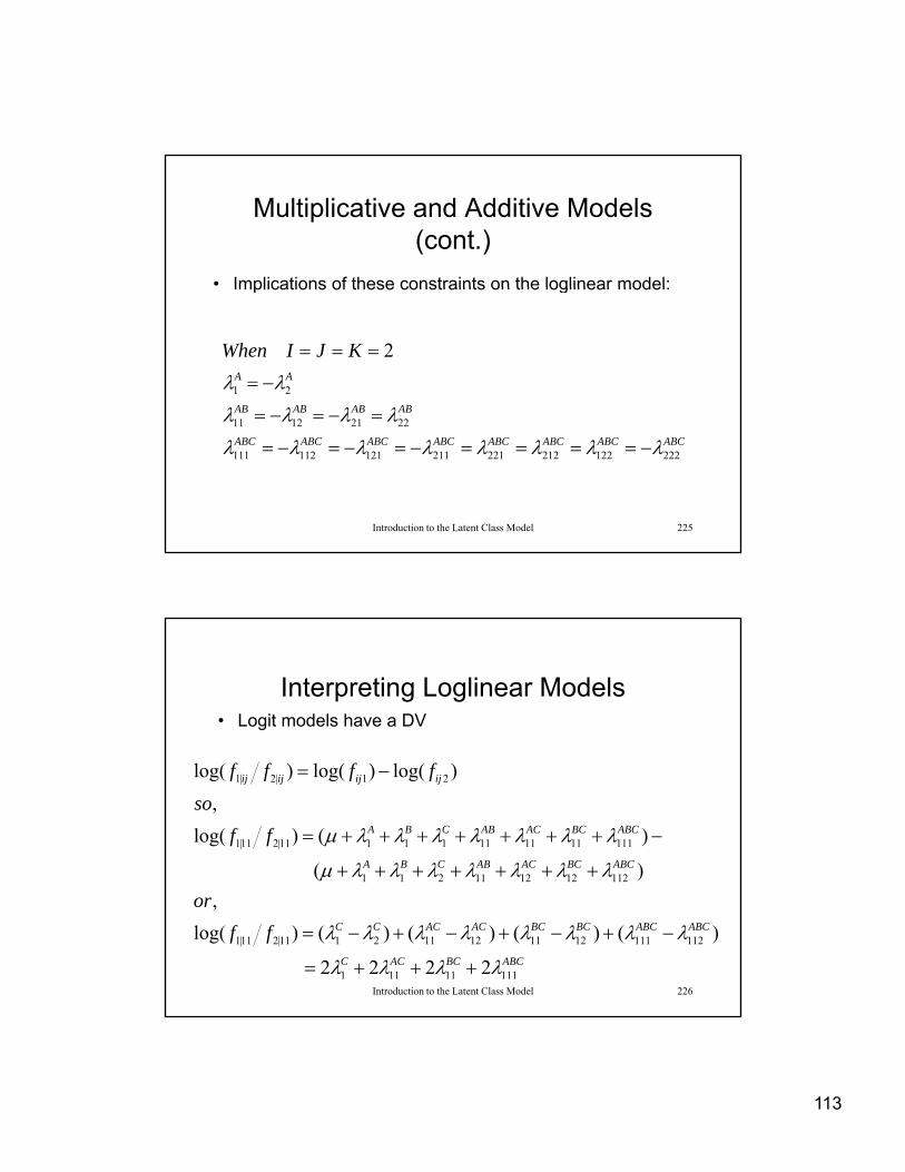
113
Multiplicative and Additive Models (cont.)
• Implications of these constraints on the loglinear model:Implications of these constraints on the loglinear model:
ABABABAB
AA
KJIWhen
22211211
21
2
Introduction to the Latent Class Model 225
ABCABCABCABCABCABCABCABC222122212221211121112111
22211211
Interpreting Loglinear Models• Logit models have a DV
ABCBCACABCBA
ABCBCACABCBA
ijijijij
ff
so
ffff
112121211211
11111111111111|211|1
21|2|1
)(
)()log(
,
)log()log()log(
Introduction to the Latent Class Model 226
ABCBCACC
ABCABCBCBCACACCCff
or
11111111
112111121112112111|211|1
2222
)()()()()log(
,
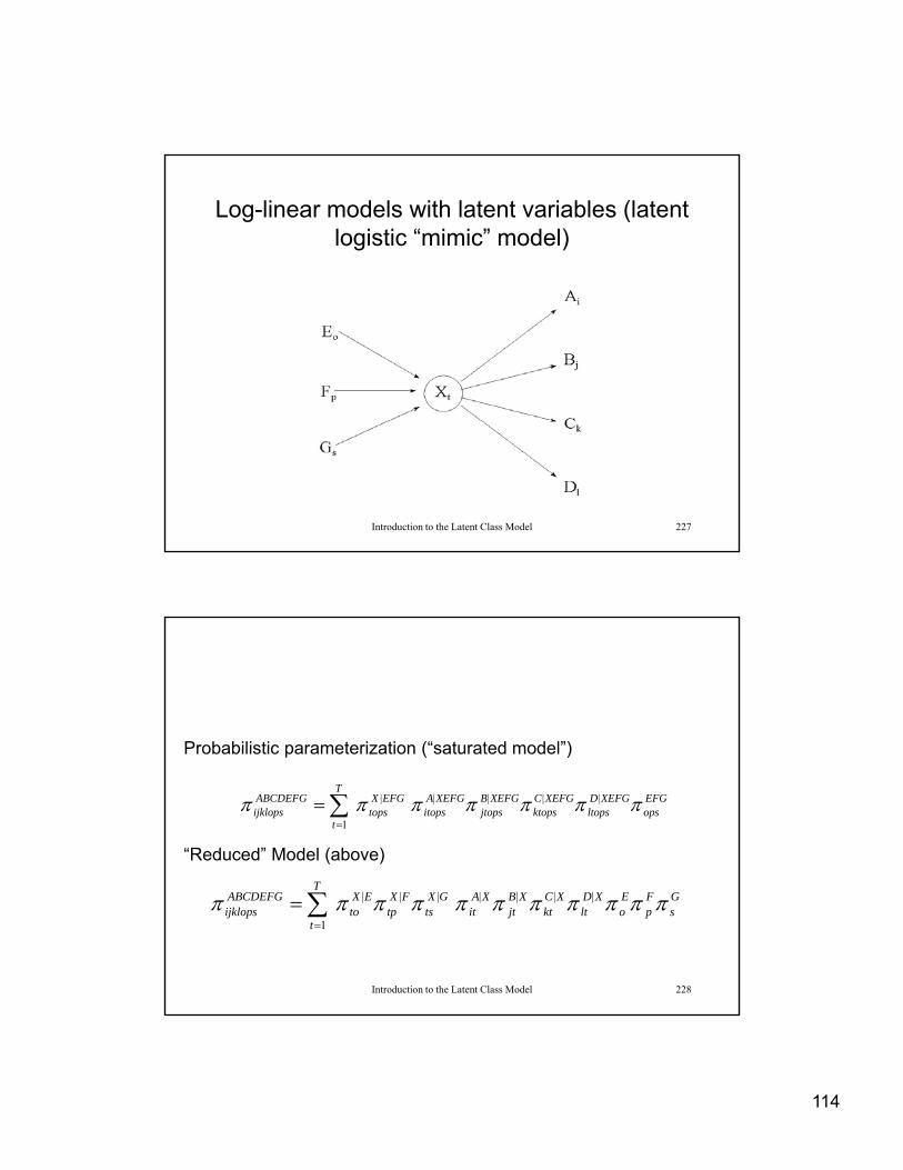
114
Log-linear models with latent variables (latent logistic “mimic” model)
Introduction to the Latent Class Model 227
Probabilistic parameterization (“saturated model”)
EFGops
XEFGDltops
XEFGCktops
XEFGBjtops
XEFGAitops
T
t
EFGXtops
ABCDEFGijklops ||||
1
|
T
Probabilistic parameterization ( saturated model )
“Reduced” Model (above)
Introduction to the Latent Class Model 228
Gs
Fp
Eo
XDlt
XCkt
XBjt
XAit
T
t
GXts
FXtp
EXto
ABCDEFGijklops ||||
1
|||
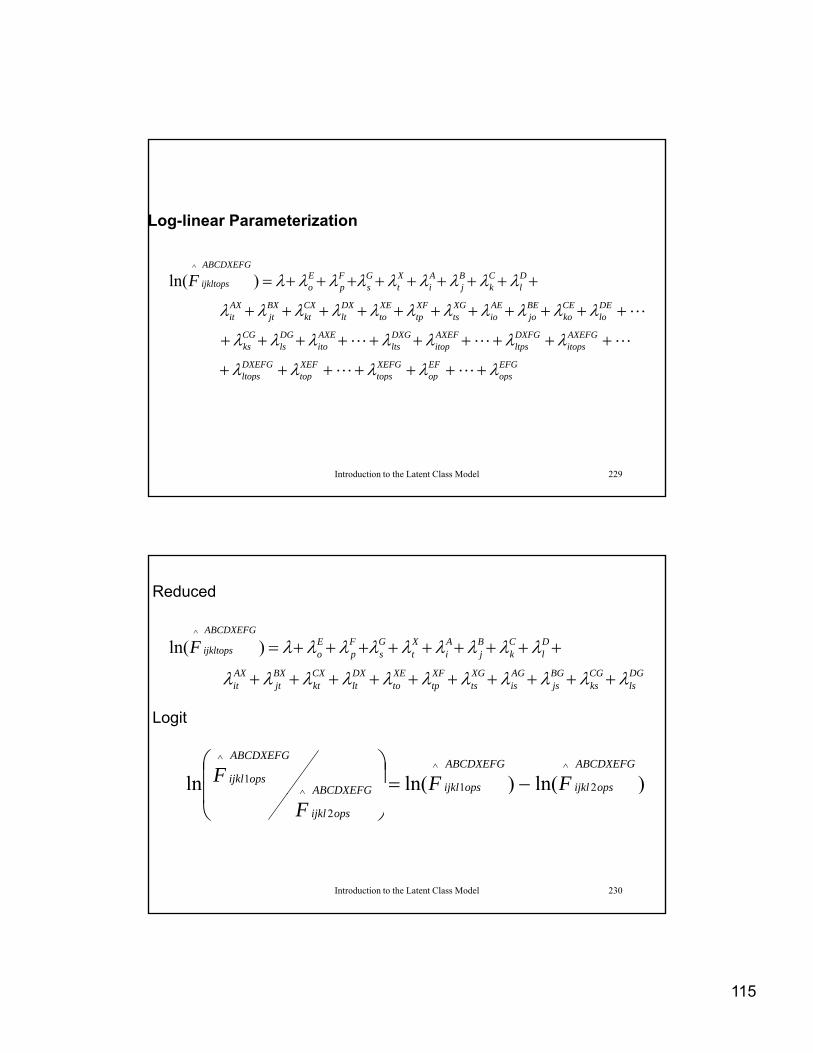
115
Log-linear Parameterization
EFGops
EFop
XEFGtops
XEFtop
DXEFGltops
AXEFGitops
DXFGltps
AXEFitop
DXGlts
AXEito
DGls
CGks
DElo
CEko
BEjo
AEio
XGts
XFtp
XEto
DXlt
CXkt
BXjt
AXit
Dl
Ck
Bj
Ai
Xt
Gs
Fp
Eo
ABCDXEFG
ijkltopsF
)ln(^
Introduction to the Latent Class Model 229
opsoptopstopltops
DGCGBGAGXGXFXEDXCXBXAX
Dl
Ck
Bj
Ai
Xt
Gs
Fp
Eo
ABCDXEFG
ijkltopsF
)ln(^
Reduced
DGls
CGks
BGjs
AGis
XGts
XFtp
XEto
DXlt
CXkt
BXjt
AXit
Logit
)ln()ln(ln 2
^
1
^
^1
^ ABCDXEFG
opsijkl
ABCDXEFG
opsijklABCDXEFG
ABCDXEFG
opsijkl FFF
Introduction to the Latent Class Model 230
)()(2opsijklF

116
For our model, this yields (recalling the identifying restrictions)
ABCDXEFG^
GXFXEXDXCX
CXBXAXXABCDXEFG
opsijkl
ABCDXEFG
opsijkl
F
F
1111111111
111111
2
^1
^
22222
2222ln
Introduction to the Latent Class Model 231
* Belief in God Latent logistic example w/ * 3 indpendent variables; order f,e,d,c,b,a* a=v31d, b=v32d, c=v33d, d=m/f, e=city, * f=w/e; city: 1=50k+, 2=5-50k, 3=lt 5klat 1man 6dim 2 2 3 2 2 2 2lab X F E D C B Amod X|DEF XD,XE,XF
A|XB|XC|XF XC,FC
dat [51 11 3 128 2 1 3 249 28 6 2 96 1 0 8 313
13 3 0 25 1 0 2 105 6 2 3 23 0 0 2 1065 0 0 12 0 0 2 54 4 0 0 18 0 0 1 74
Introduction to the Latent Class Model 232
0 18 0 0 1 74138 14 3 26 2 0 0 39 129 15
4 50 0 1 2 64117 14 9 24 0 0 2 56 99 14 11 40 1 1 2 85
109 11 5 46 1 1 0 58 82 14 5 61 1 1 1 111 ]

117
X-squared = 81.1028 (0.2166)
L-squared = 85.3247 (0.1350)
Cressie-Read = 80.5868 (0.2284)
Dissimilarity index = 0.0519
Degrees of freedom = 72
Log-likelihood = -9959.26854
Number of parameters = 12 (+12)
Introduction to the Latent Class Model 233
Sample size = 2832.0
BIC(L-squared) = -486.9844
AIC(L-squared) = -58.6753
* P(A|X) *
1 | 1 0.8834 (0.0111)
1 | 2 0.0179 (0.0035)
* P(B|X) *
1 | 1 0.9562 (0.0081)
1 | 2 0.0026 (0.0019)
* P(C|XF) *
1 | 1 1 0.9808 (0.0065)
2 | 1 1 0.0192 (0.0065)
1 | 1 2 0.9892 (0.0036)
2 | 1 2 0.0108 (0.0036)
Introduction to the Latent Class Model 234
1 | 2 1 0.2487 (0.0124)
2 | 2 1 0.7513 (0.0124)
1 | 2 2 0.3731 (0.0189)
2 | 2 2 0.6269 (0.0189)

118
* P(X|FED) *
1 | 1 1 1 0.1458 (0.0129)
1 | 1 1 2 0.0811 (0.0084)
1 | 1 2 1 0.1111 (0.0133)
1 | 1 2 2 0.0607 (0.0083)
1 | 1 3 1 0.0746 (0.0099)
1 | 1 3 2 0.0400 (0.0059)
1 | 2 1 1 0.7107 (0.0215)
1 | 2 1 2 0 5596 (0 0239)
* Belief in God Latent logistic example w/
* a=v31d, b=v32d, c=v33d, 1 | 2 1 2 0.5596 (0.0239)
1 | 2 2 1 0.6428 (0.0238)
1 | 2 2 2 0.4821 (0.0248)
1 | 2 3 1 0.5373 (0.0255)
1 | 2 3 2 0.3752 (0.0234)
2 | 1 1 1 0.8542 (0.0129)
2 | 1 1 2 0.9189 (0.0084)
2 | 1 2 1 0.8889 (0.0133)
2 | 1 2 2 0.9393 (0.0083)
d=m/f, e=city,
* f=w/e; city: 1=50k+, 2=5-50k, 3=lt 5k
Introduction to the Latent Class Model 235
| ( )
2 | 1 3 1 0.9254 (0.0099)
2 | 1 3 2 0.9600 (0.0059)
2 | 2 1 1 0.2893 (0.0215)
2 | 2 1 2 0.4404 (0.0239)
2 | 2 2 1 0.3572 (0.0238)
2 | 2 2 2 0.5179 (0.0248)
2 | 2 3 1 0.4627 (0.0255)
2 | 2 3 2 0.6248 (0.0234)
Models for Analyzing Categorically-Scored Panel Data
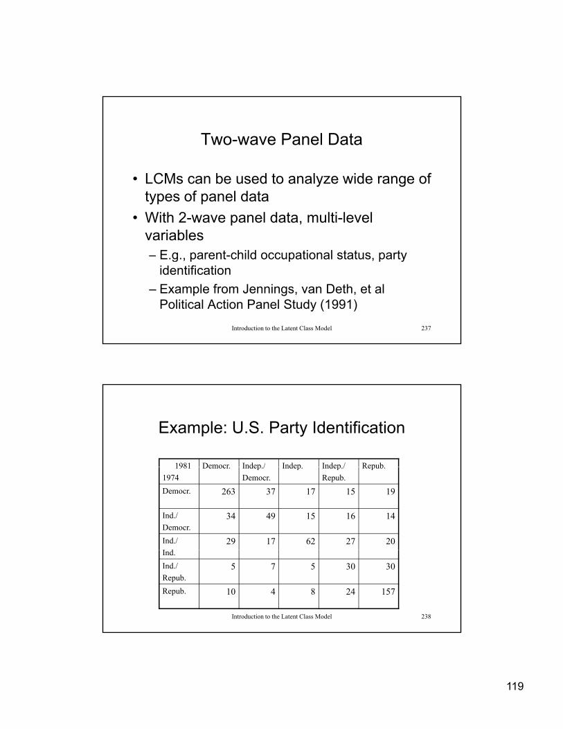
119
Two-wave Panel Data
• LCMs can be used to analyze wide range of• LCMs can be used to analyze wide range of types of panel data
• With 2-wave panel data, multi-level variables– E.g., parent-child occupational status, party
Introduction to the Latent Class Model 237
g p p p yidentification
– Example from Jennings, van Deth, et al Political Action Panel Study (1991)
Example: U.S. Party Identification
1981 Democr Indep / Indep Indep / Repub1981
1974
Democr. Indep./
Democr.
Indep. Indep./
Repub.
Repub.
Democr. 263 37 17 15 19
Ind./
Democr.34 49 15 16 14
Ind./
I d29 17 62 27 20
Introduction to the Latent Class Model 238
Ind.
Ind./
Repub.5 7 5 30 30
Repub. 10 4 8 24 157
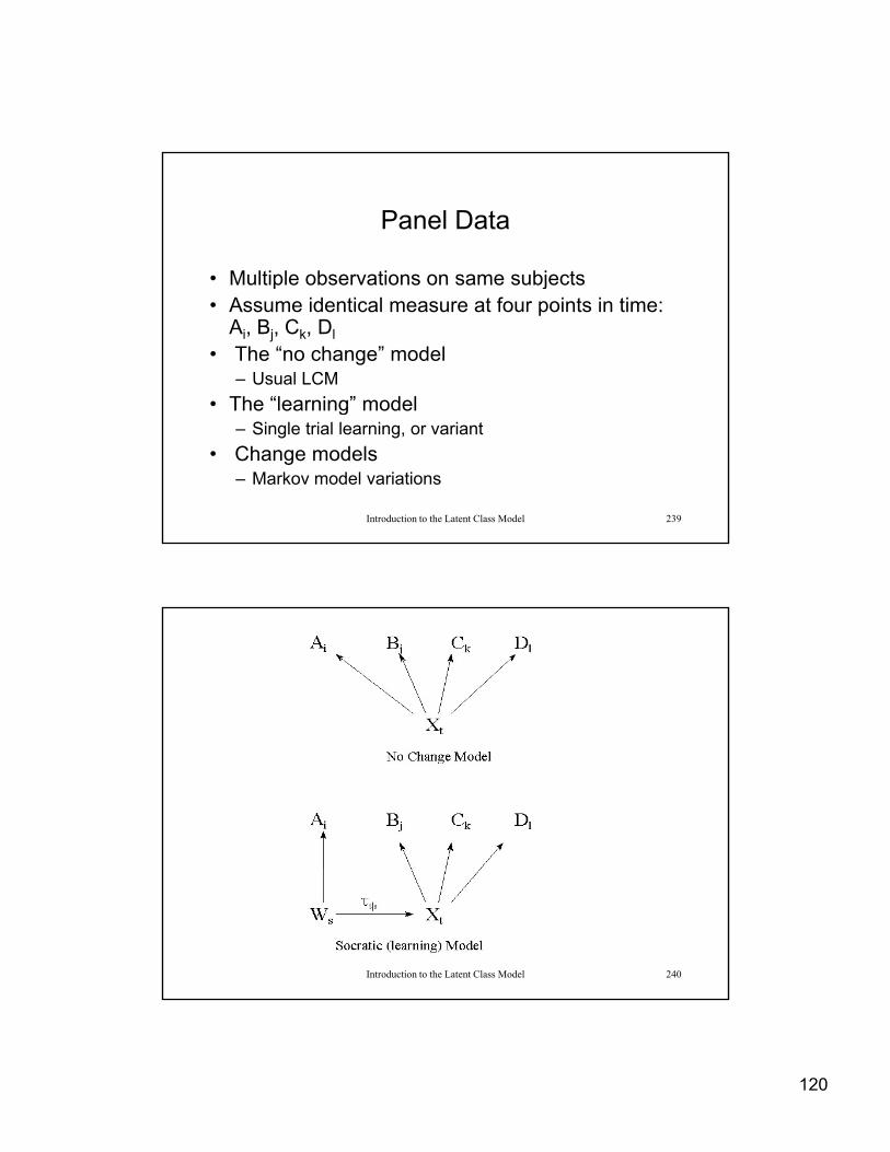
120
Panel Data
• Multiple observations on same subjectsMultiple observations on same subjects• Assume identical measure at four points in time:
Ai, Bj, Ck, Dl
• The “no change” model– Usual LCM
• The “learning” model
Introduction to the Latent Class Model 239
g– Single trial learning, or variant
• Change models– Markov model variations
Introduction to the Latent Class Model 240
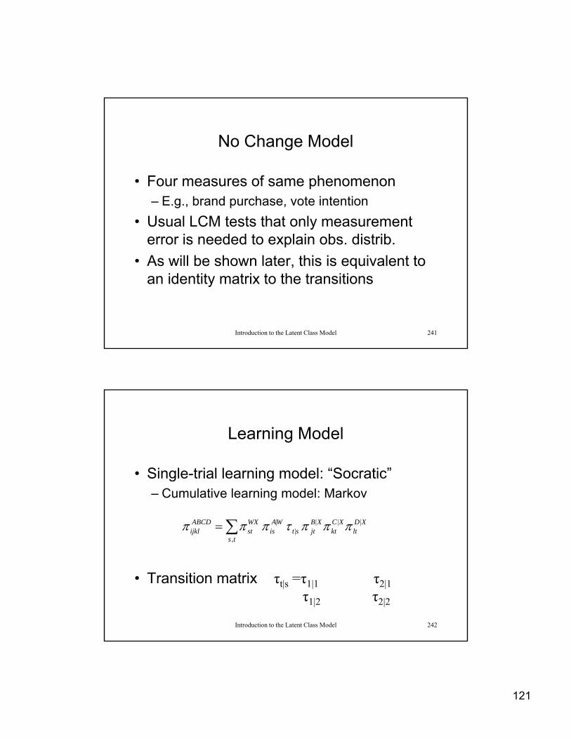
121
No Change Model
• Four measures of same phenomenon• Four measures of same phenomenon– E.g., brand purchase, vote intention
• Usual LCM tests that only measurement error is needed to explain obs. distrib.
• As will be shown later, this is equivalent to
Introduction to the Latent Class Model 241
As will be shown later, this is equivalent to an identity matrix to the transitions
Learning Model
• Single trial learning model: “Socratic”• Single-trial learning model: Socratic – Cumulative learning model: Markov
XDlt
XCkt
XBjtst
ts
WAis
WXst
ABCDijkl
||||
,
|
Introduction to the Latent Class Model 242
• Transition matrix τt|s =τ1|1 τ2|1
τ1|2 τ2|2
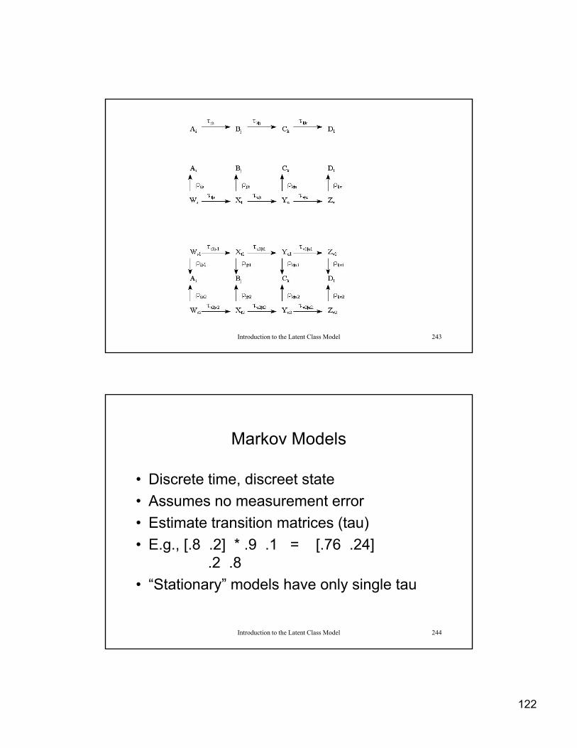
122
Introduction to the Latent Class Model 243
Markov Models
• Discrete time discreet state• Discrete time, discreet state
• Assumes no measurement error
• Estimate transition matrices (tau)
• E.g., [.8 .2] * .9 .1 = [.76 .24]2 8
Introduction to the Latent Class Model 244
.2 .8
• “Stationary” models have only single tau
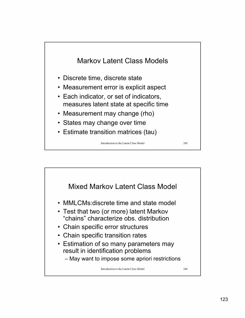
123
Markov Latent Class Models
• Discrete time discrete state• Discrete time, discrete state
• Measurement error is explicit aspect
• Each indicator, or set of indicators, measures latent state at specific time
• Measurement may change (rho)
Introduction to the Latent Class Model 245
• Measurement may change (rho)
• States may change over time
• Estimate transition matrices (tau)
Mixed Markov Latent Class Model
• MMLCMs:discrete time and state modelMMLCMs:discrete time and state model• Test that two (or more) latent Markov
“chains” characterize obs. distribution• Chain specific error structures• Chain specific transition rates
Introduction to the Latent Class Model 246
• Estimation of so many parameters may result in identification problems– May want to impose some apriori restrictions

124
Mixed Markov Latent Class Models
• Let delta (r) represent the latent chainsLet delta (r) represent the latent chains
• Let rho represent the measurement of the
R
r
I
i
J
j
K
k
L
lvrlurvrurktrurtrjsrtrsrir
ABCDijkl
1 1 1 1 1|||||||
Introduction to the Latent Class Model 247
platent states
• Let tau represent the latent transition matrices
British Election Study Panel Data
1993, 1995, 1996, 1997
Conservative, Labor, Other
296 2 10 3 2 0 7 1 12 0 0 2 5 1 0 0 112 2 4 0 1 0 7 1 133 0 0 0 1 0 0 0 00 0 1 4 345 11 1 10 6
Introduction to the Latent Class Model 248
0 0 1 4 345 11 1 10 60 0 0 1 9 2 0 6 915 0 4 1 1 0 3 0 20 2 0 2 31 6 0 4 89 1 4 0 5 8 14 14 155

125
Mixed Markov Latent Class Model: Mover-Stayer Model
df 45, indep.pars 35+0, LR 36.228, Chi-2 41.915, AIC 4935.9, BIC 5110.1
chain proportions
0.290276596 0.709723404
Introduction to the Latent Class Model 249
initial probabilities of group 1,
chain 1 0.241333496 0.424339960 0.334326544chain 2 0.414382039 0.371593932 0.214024029
Mixed Markov Latent Class Model: Mover-Stayer Model (cont.)
Time homogeneous response probabilities (restriction)
response probs., group 1, , chain 1, indicator/wave 1 class 1 0.817388460 0.000005902 0.182605638class 2 0.013193300 0.850936789 0.135869912class 3 0.038748266 0.000000000 0.961251734
b 1 h i 2 i di t / 1
Introduction to the Latent Class Model 250
response probs., group 1, , chain 2, indicator/wave 1 class 1 0.974524046 0.007899203 0.017576751class 2 0.000000000 0.999954341 0.000045659class 3 0.000000063 0.063325785 0.936674153

126
Mixed Markov Latent Class Model: Mover-Stayer Model (cont.)
transition probs., group 1, , chain 1, indicators/waves 1, 2 class 1 0.458222021 0.113550651 0.428227327class 2 0.000000000 1.000000000 0.000000000class 3 0.142601921 0.328780884 0.528617194
transition probs., group 1, , chain 1, indicators/waves 2, 3 class 1 0.912941878 0.087057889 0.000000233class 2 0.000000000 0.964913867 0.035086133
Introduction to the Latent Class Model 251
class 3 0.243960957 0.000000520 0.756038523
transition probs., group 1, , chain 1, indicators/waves 3, 4 class 1 0.820655669 0.066646082 0.112698249class 2 0.057896931 0.937648068 0.004455001class 3 0.291538432 0.075361473 0.633100094
Mixed Markov Latent Class Model: Mover-Stayer Model (cont.)
transition probs., group 1, , chain 2, indicators/waves 1, 2 class 1 1.000000000 0.000000000 0.000000000class 2 0.000000000 1.000000000 0.000000000class 3 0.000000000 0.000000000 1.000000000
transition probs., group 1, , chain 2, indicators/waves 2, 3 class 1 1.000000000 0.000000000 0.000000000class 2 0.000000000 1.000000000 0.000000000
Introduction to the Latent Class Model 252
class 3 0.000000000 0.000000000 1.000000000
transition probs., group 1, , chain 2, indicators/waves 3, 4 class 1 1.000000000 0.000000000 0.000000000class 2 0.000000000 1.000000000 0.000000000class 3 0.000000000 0.000000000 1.000000000


![9. Heterogeneity: Latent Class Modelspeople.stern.nyu.edu › wgreene › DiscreteChoice › 2014 › DC2014-9-LCModels.pdf[Topic 9-Latent Class Models] 3/66 Latent Classes • A population](https://img.pdfslide.net/doc/110x75/5f03e2617e708231d40b3e43/9-heterogeneity-latent-class-a-wgreene-a-discretechoice-a-2014-a-dc2014-9-lcmodelspdf.jpg)