An iterative optimisation procedure for the rehabilitation

Available on website http://www.wrc.org.zaISSN 0378-4738 = Water SA Vol. 34 No. 2 April 2008ISSN 1816-7950 = Water SA (on-line)

225

* To whom all correspondence should be addressed. +55-83-3216.7037; fax: +55-83-3216.7037;e-mail: [email protected] 24 August 2006; accepted in revised form 21 January 2008.

An iterative optimisation procedure for the rehabilitation of water-supply pipe networks

Heber Pimentel Gomes1*; Saulo de Tarso Marques Bezerra2 and Vajapeyam Srirangachar Srinivasan3

1Department of Civil Engineering, Federal University of Paraíba, Campus I, UFPB, João Pessoa, Brazil2 Former graduate student, Department of Civil Engineering, Federal University of Campina Grande, Campus I, 58109-900

Campina Grande, PB,Brazil3 Department of Civil Engineering, Federal University of Campina Grande, Campus I, 58109-900 Campina Grande, PB,Brazil

Abstract

This paper presents an iterative method for the optimisation of the total costs for the rehabilitation of water-supply pipe net-works with flow and pressure deficiency at the consumer nodes. The procedure is based on the exchange gradient concept of Granados for the economic design of pressurised networks. The substitution of pipe sections, relining and increase in pump-ing head are considered as being rehabilitation options. An initial solution is obtained for the deficient network by determining the required pumping head that would meet the pressure and discharge requirements at all the nodes. Subsequently, the pump-ing head is reduced in stages and for each reduction; the network of minimum cost is obtained by the substitution or relining of individual pipes in part or in full. The optimal solution is reached when the marginal annual cost of pipe rehabilitation exceeds the reduction in annual pumping costs.

Keywords: rehabilitation, networks, optimisation models, pipe networks

Notation

C Hazen-Williams’ coefficient CE present value of the total cost of energy for pumpingCp annual cost of electrical power Cp’t present value of the annual pumping cost for the yearCpt annual pumping cost for the year ‘t’D internal diameter of the pipee annual rate of increase in the unit cost of energyEP excess of available pressure headEPmin minimum of the excesses of available pressure headsFa present worth factorG exchange gradient valueG* the optimum value of the Exchange gradientGe the energy cost gradientHf head lossi annual interest or discount rateL length of the pipenb number of the hours of pumping per annum P power required for the motor-pump unitP1 initial costP2 cost of substitution or rehabilitation of the pipePh pressure headPm power required for pumping to raise the head by unit valuept unit cost of electrical energyQ flow rate in the pipeT* potential sectionZj supply reservoir level for the year ‘j’ΔHf reduction in the loss of head obtained by the rehabilitation optionη efficiency of the pump-motor unit

Introduction

The basic objective of all water-supply pipe networks is to meet the flow demands at the nodes subject to a minimum pressure requirement. Even when a network is initially designed to meet all the current demands and the expected increases within a rea-sonable future, often the networks fail to meet the flow and pres-sure requirements over time. This could be due to either a higher than expected rise in flow demand or due to the deterioration of the network or a combination of both. Older systems are also liable to breaks and leakage that will add to the flow deficiencies and unsatisfactory performance of the network. While some of the problems could be alleviated with regular care and main-tenance, slow and continuous deterioration of the pipes due to corrosion, encrustation and other problems cannot be avoided altogether. Hence, the rehabilitation of water-supply networks to meet the demand is a major task for the water-supply agencies and selecting a cost-effective method that will restore or update the system is of utmost importance. The total cost of rehabilita-tion, in general, consists of the initial cost of repairs or substi-tutions, annual pumping costs and maintenance costs. During the lifetime of the network, in the majority of cases, the energy cost of pumping surpasses the investment costs of the network and other installations. The maintenance costs, however, may be assumed to be common and similar in all scenarios and hence excluded from the optimisation process. For a water-supply pipe network with flow and pressure deficiencies at the consumer nodes, the options of rehabilitation include:

Repairing and cleaning of pipes• Replacement of or addition of parallel pipes• Increasing the supply pressure/static head. •

Obviously, these options do not exclude one another and all types of combinations could be considered in order to obtain the con-figuration of minimum capital and operating costs. Considering the expected period of the useful life of the rehabilitated net-

mailto:[email protected]

Available on website http://www.wrc.org.zaISSN 0378-4738 = Water SA Vol. 34 No. 2 April 2008

ISSN 1816-7950 = Water SA (on-line)

226

work, the options could be compared on the basis of the present-day cost to obtain the minimum value. Hence, the economic analysis utilised in this paper for the decision process considers the costs of the physical interventions that are necessary as well as the operating pumping costs based on the electrical energy demanded by the system.

Literature review

The subject of rehabilitation of water-supply networks and the best scheme that can be evolved has been extensively investi-gated over the past three decades. The past investigations can be grouped into three different categories: The first, in which an attempt is made to predict when and where a failure in the network might occur (Shamir and Howard, 1979; Sinske and Zietsman, 2004); the second, in which the aim is to minimise the total cost of the rehabilitated network (Halhal et al., 1997; Zecchin et al., 2007); and the third, that aims at combining the aforementioned two groups. An adequate strategy of rehabilitation must lead to a reliable supply that is cost efficient. The rehabilitation itself could be either the substitution of individual pipes or an appro-priate relining of the interior surface. The adopted strategy could be for individual pipes or for the entire system. In the former case, the impact of rehabilitation over the network is evaluated by a posterior system analysis, while in the latter case, the implied decisions of individual units are considered explicitly in the strategy. Lansey et al. (1992) used an optimi-sation procedure using a reduced gradient technique to estab-lish a rehabilitation schedule for the present time and a future period of 10 years taking into account the projected demands during that period. In their strategy replacement or lining of parts of the length of a pipe with or without a change in diam-eter were considered admitting that in process any section of a pipe could be left as it is. Walski (2001) discusses some of the compelling problems facing optimisation and why, contrary to the expectations in the decades of 1980 and 1990, these models are not used regu-larly by the practising engineer. He concludes that this is so due to the following limitations of the methods based on cost minimisation:

The uncertainty of future demand • Existence of many alternatives with virtually the same net • benefitsActual demands tend to be controlled to a certain extent by • the sizing of pipes.

Currently, genetic algorithms are used frequently in the opti-misation of water distribution systems. Cheung et al. (2003) presents a comparative study of two multi-objective evolu-tionary methods, namely, multi-objective genetic algorithm (MOGA) and strength Pareto evolutionary algorithm (SPEA) for the rehabilitation of networks. The analyses were conducted on a simple hypothetical network for cost minimisation and mini-mum pressure requirement. Ndiritu (2005) utilised genetic algo-rithms and presents an approach for determining the reservoir sizes and monthly operating rules that maximise the yield of a water-supply system subject to multiple reliability constraints of supply and reservoir storage. A behavioural analysis model linked to a genetic algorithm is applied and the constraints are implemented using multiplicative penalties. However, in spite of the great evolution of computing power over the years, the long processing time that is required remains a major disadvantage of these methods. Cui and Kuczera (2003) highlight this problem

of long computation times and propose that such analyses be handled by super computers or by parallel computation. Zecchin et al. (2006) utilised a new technique called the ant colony optimisation (ACO) to water distribution systems which is based on the analogy of the behaviour of a colony of foraging ants, and their ability to determine the shortest route between their nest and a food source. This algorithm envisages local searching around the best solution found in each iteration, while implementing methods that slow convergence and facili-tate further exploration. This method yielded good results when compared with others. Thus, rehabilitation strategies that adopt sophisticated opti-misation techniques considering present and future demand as well as all the expected constraints do not necessarily lead to practicable strategies that are cost-efficient. With this in mind, a relatively straightforward and iterative procedure for the reha-bilitation of water-supply networks is proposed herein.

Methodology

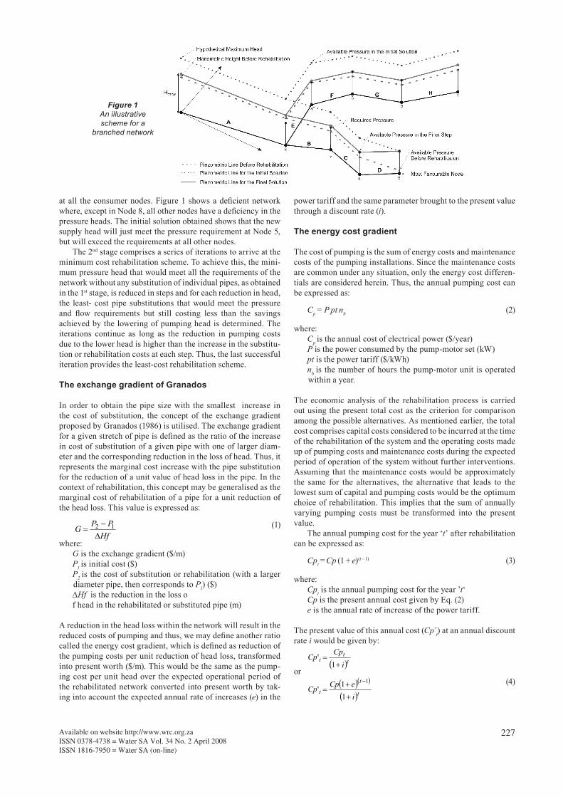
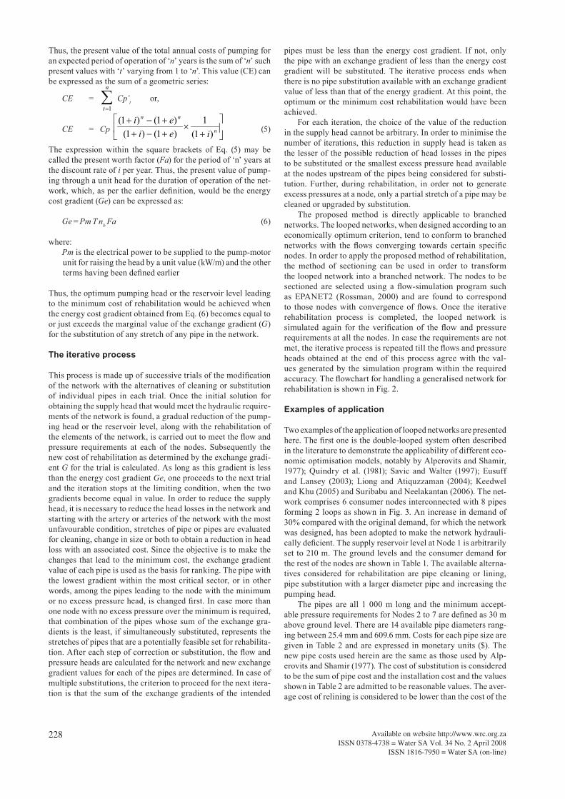
The process of rehabilitation of pipe networks may be divided into two distinct phases: namely, the diagnostic phase and the rehabilitation phase. A detailed initial diagnosis of the system is a crucial phase as this will determine what elements of the system need immediate or future rehabilitation through a thor-ough description of the physical and hydraulic characteristics of the network. This information can be generated from the maintenance records of the system and by the use of one of the calibration models (Walski, 1983; Silva, 2003; Jiménez et al., 2004; Kapelan et al., 2007; and many others), that would provide the actual values of the hydraulic parameters like the Hazen-Williams coefficients of the pipe units, the nodal pressures and flow discharges. This information along with the current and expected demands of the network would form the basis for the rehabilitation scheme. The economic analysis of rehabilitation must take into account the total cost involved in the form of the initial capi-tal cost and the operational and maintenance costs. All costs incurred with the fixed components like pipes and pumps are considered capital costs while the periodic maintenance and pumping costs are considered here as operating costs. In order to obtain the optimum selection, all costs are converted to present worth through the application of discount rates for future expenditure and the expected increases in energy rates for the future power consumption. The procedure is based on the exchange gradient criterion of Granados (1986) and can be divided into two stages. In the 1st stage, the existing network is made to meet the flow and pressure requirements at all nodes considering the pumping head or the reservoir level of a single loading system as the only variable and the minimum head that would attend all the requirements of the system would be the initial value of the maximum pumping head. An illustrative scheme is shown in Fig. 1 for a branched network. The algorithm utilised for this stage consists of determin-ing the fictitious minimum head required at the loading point to attend the flow and pressure requirements at each of the nodes. This fictitious minimum head is obtained as a sum of the eleva-tion of the pipe at the node, the pressure head required at the node and the sum of all the head losses in the upstream pipes up to the node for the required flow. The highest value of the fictitious heads thus obtained for all the nodes would then con-stitute the initial solution or the pumping head or reservoir level required at the source to attend the requirements of the network


227

at all the consumer nodes. Figure 1 shows a deficient network where, except in Node 8, all other nodes have a deficiency in the pressure heads. The initial solution obtained shows that the new supply head will just meet the pressure requirement at Node 5, but will exceed the requirements at all other nodes. The 2nd stage comprises a series of iterations to arrive at the minimum cost rehabilitation scheme. To achieve this, the mini-mum pressure head that would meet all the requirements of the network without any substitution of individual pipes, as obtained in the 1st stage, is reduced in steps and for each reduction in head, the least- cost pipe substitutions that would meet the pressure and flow requirements but still costing less than the savings achieved by the lowering of pumping head is determined. The iterations continue as long as the reduction in pumping costs due to the lower head is higher than the increase in the substitu-tion or rehabilitation costs at each step. Thus, the last successful iteration provides the least-cost rehabilitation scheme.

The exchange gradient of Granados

In order to obtain the pipe size with the smallest increase in the cost of substitution, the concept of the exchange gradient proposed by Granados (1986) is utilised. The exchange gradient for a given stretch of pipe is defined as the ratio of the increase in cost of substitution of a given pipe with one of larger diam-eter and the corresponding reduction in the loss of head. Thus, it represents the marginal cost increase with the pipe substitution for the reduction of a unit value of head loss in the pipe. In the context of rehabilitation, this concept may be generalised as the marginal cost of rehabilitation of a pipe for a unit reduction of the head loss. This value is expressed as:

(1)

where: G is the exchange gradient ($/m) P1 is initial cost ($) P2 is the cost of substitution or rehabilitation (with a larger

diameter pipe, then corresponds to P1) ($) ∆Hf is the reduction in the loss o f head in the rehabilitated or substituted pipe (m)

A reduction in the head loss within the network will result in the reduced costs of pumping and thus, we may define another ratio called the energy cost gradient, which is defined as reduction of the pumping costs per unit reduction of head loss, transformed into present worth ($/m). This would be the same as the pump-ing cost per unit head over the expected operational period of the rehabilitated network converted into present worth by tak-ing into account the expected annual rate of increases (e) in the

power tariff and the same parameter brought to the present value through a discount rate (i).

The energy cost gradient

The cost of pumping is the sum of energy costs and maintenance costs of the pumping installations. Since the maintenance costs are common under any situation, only the energy cost differen-tials are considered herein. Thus, the annual pumping cost can be expressed as:

Cp = P pt nb (2)

where: Cp is the annual cost of electrical power ($/year) P is the power consumed by the pump-motor set (kW) pt is the power tariff ($/kWh) nb is the number of hours the pump-motor unit is operated

within a year.

The economic analysis of the rehabilitation process is carried out using the present total cost as the criterion for comparison among the possible alternatives. As mentioned earlier, the total cost comprises capital costs considered to be incurred at the time of the rehabilitation of the system and the operating costs made up of pumping costs and maintenance costs during the expected period of operation of the system without further interventions. Assuming that the maintenance costs would be approximately the same for the alternatives, the alternative that leads to the lowest sum of capital and pumping costs would be the optimum choice of rehabilitation. This implies that the sum of annually varying pumping costs must be transformed into the present value. The annual pumping cost for the year ‘t’ after rehabilitation can be expressed as:

Cpt = Cp (1 + e)(t – 1) (3)

where: Cpt is the annual pumping cost for the year ’t‘ Cp is the present annual cost given by Eq. (2) e is the annual rate of increase of the power tariff.

The present value of this annual cost (Cp’t) at an annual discount rate i would be given by:

or (4)

Figure 1An illustrative scheme for a

branched network

HfPPG

12

tt

ti

CpCp

1

'

tt

tieCpCp

11'

1



228

Thus, the present value of the total annual costs of pumping for an expected period of operation of ‘n’ years is the sum of ‘n’ such present values with ‘t’ varying from 1 to ‘n’. This value (CE) can be expressed as the sum of a geometric series:

CE = Cp’t or,

CE = Cp (5)

The expression within the square brackets of Eq. (5) may be called the present worth factor (Fa) for the period of ‘n’ years at the discount rate of i per year. Thus, the present value of pump-ing through a unit head for the duration of operation of the net-work, which, as per the earlier definition, would be the energy cost gradient (Ge) can be expressed as:

Ge = Pm T nb Fa (6)

where: Pm is the electrical power to be supplied to the pump-motor

unit for raising the head by a unit value (kW/m) and the other terms having been defined earlier

Thus, the optimum pumping head or the reservoir level leading to the minimum cost of rehabilitation would be achieved when the energy cost gradient obtained from Eq. (6) becomes equal to or just exceeds the marginal value of the exchange gradient (G) for the substitution of any stretch of any pipe in the network.

The iterative process

This process is made up of successive trials of the modification of the network with the alternatives of cleaning or substitution of individual pipes in each trial. Once the initial solution for obtaining the supply head that would meet the hydraulic require-ments of the network is found, a gradual reduction of the pump-ing head or the reservoir level, along with the rehabilitation of the elements of the network, is carried out to meet the flow and pressure requirements at each of the nodes. Subsequently the new cost of rehabilitation as determined by the exchange gradi-ent G for the trial is calculated. As long as this gradient is less than the energy cost gradient Ge, one proceeds to the next trial and the iteration stops at the limiting condition, when the two gradients become equal in value. In order to reduce the supply head, it is necessary to reduce the head losses in the network and starting with the artery or arteries of the network with the most unfavourable condition, stretches of pipe or pipes are evaluated for cleaning, change in size or both to obtain a reduction in head loss with an associated cost. Since the objective is to make the changes that lead to the minimum cost, the exchange gradient value of each pipe is used as the basis for ranking. The pipe with the lowest gradient within the most critical sector, or in other words, among the pipes leading to the node with the minimum or no excess pressure head, is changed first. In case more than one node with no excess pressure over the minimum is required, that combination of the pipes whose sum of the exchange gra-dients is the least, if simultaneously substituted, represents the stretches of pipes that are a potentially feasible set for rehabilita-tion. After each step of correction or substitution, the flow and pressure heads are calculated for the network and new exchange gradient values for each of the pipes are determined. In case of multiple substitutions, the criterion to proceed for the next itera-tion is that the sum of the exchange gradients of the intended

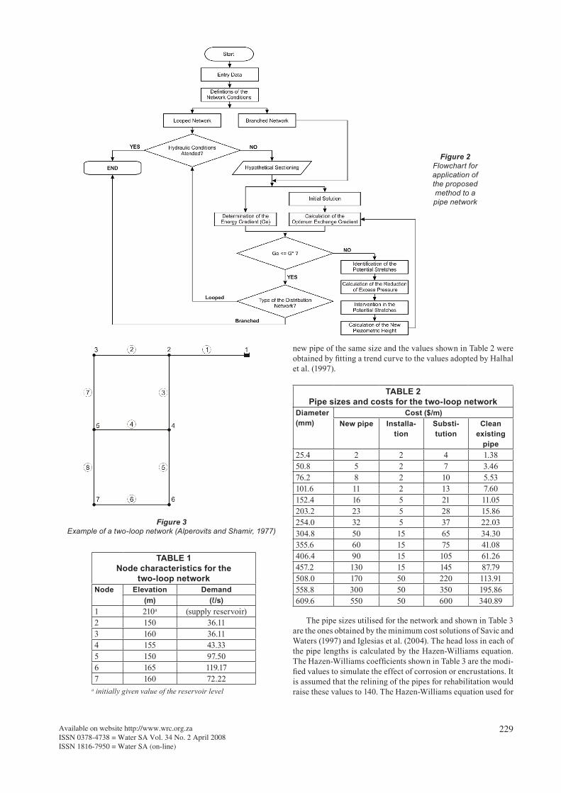
pipes must be less than the energy cost gradient. If not, only the pipe with an exchange gradient of less than the energy cost gradient will be substituted. The iterative process ends when there is no pipe substitution available with an exchange gradient value of less than that of the energy gradient. At this point, the optimum or the minimum cost rehabilitation would have been achieved. For each iteration, the choice of the value of the reduction in the supply head cannot be arbitrary. In order to minimise the number of iterations, this reduction in supply head is taken as the lesser of the possible reduction of head losses in the pipes to be substituted or the smallest excess pressure head available at the nodes upstream of the pipes being considered for substi-tution. Further, during rehabilitation, in order not to generate excess pressures at a node, only a partial stretch of a pipe may be cleaned or upgraded by substitution. The proposed method is directly applicable to branched networks. The looped networks, when designed according to an economically optimum criterion, tend to conform to branched networks with the flows converging towards certain specific nodes. In order to apply the proposed method of rehabilitation, the method of sectioning can be used in order to transform the looped network into a branched network. The nodes to be sectioned are selected using a flow-simulation program such as EPANET2 (Rossman, 2000) and are found to correspond to those nodes with convergence of flows. Once the iterative rehabilitation process is completed, the looped network is simulated again for the verification of the flow and pressure requirements at all the nodes. In case the requirements are not met, the iterative process is repeated till the flows and pressure heads obtained at the end of this process agree with the val-ues generated by the simulation program within the required accuracy. The flowchart for handling a generalised network for rehabilitation is shown in Fig. 2.

Examples of application

Two examples of the application of looped networks are presented here. The first one is the double-looped system often described in the literature to demonstrate the applicability of different eco-nomic optimisation models, notably by Alperovits and Shamir, 1977); Quindry et al. (1981); Savic and Walter (1997); Eusuff and Lansey (2003); Liong and Atiquzzaman (2004); Keedwel and Khu (2005) and Suribabu and Neelakantan (2006). The net-work comprises 6 consumer nodes interconnected with 8 pipes forming 2 loops as shown in Fig. 3. An increase in demand of 30% compared with the original demand, for which the network was designed, has been adopted to make the network hydrauli-cally deficient. The supply reservoir level at Node 1 is arbitrarily set to 210 m. The ground levels and the consumer demand for the rest of the nodes are shown in Table 1. The available alterna-tives considered for rehabilitation are pipe cleaning or lining, pipe substitution with a larger diameter pipe and increasing the pumping head. The pipes are all 1 000 m long and the minimum accept-able pressure requirements for Nodes 2 to 7 are defined as 30 m above ground level. There are 14 available pipe diameters rang-ing between 25.4 mm and 609.6 mm. Costs for each pipe size are given in Table 2 and are expressed in monetary units ($). The new pipe costs used herein are the same as those used by Alp-erovits and Shamir (1977). The cost of substitution is considered to be the sum of pipe cost and the installation cost and the values shown in Table 2 are admitted to be reasonable values. The aver-age cost of relining is considered to be lower than the cost of the

n

t 1

n

nn

ieiei

)1(1

)1()1()1()1(


229

new pipe of the same size and the values shown in Table 2 were obtained by fitting a trend curve to the values adopted by Halhal et al. (1997).

TABLE 2Pipe sizes and costs for the two-loop network

Diameter(mm)

Cost ($/m) New pipe Installa-

tionSubsti-tution

Clean existing

pipe25.4 2 2 4 1.3850.8 5 2 7 3.4676.2 8 2 10 5.53101.6 11 2 13 7.60152.4 16 5 21 11.05203.2 23 5 28 15.86254.0 32 5 37 22.03304.8 50 15 65 34.30355.6 60 15 75 41.08406.4 90 15 105 61.26457.2 130 15 145 87.79508.0 170 50 220 113.91558.8 300 50 350 195.86609.6 550 50 600 340.89

The pipe sizes utilised for the network and shown in Table 3 are the ones obtained by the minimum cost solutions of Savic and Waters (1997) and Iglesias et al. (2004). The head loss in each of the pipe lengths is calculated by the Hazen-Williams equation. The Hazen-Williams coefficients shown in Table 3 are the modi-fied values to simulate the effect of corrosion or encrustations. It is assumed that the relining of the pipes for rehabilitation would raise these values to 140. The Hazen-Williams equation used for

Figure 2Flowchart for application of the proposed method to a pipe network

Figure 3Example of a two-loop network (Alperovits and Shamir, 1977)

TABLE 1Node characteristics for the

two-loop networkNode Elevation Demand

(m) (ℓ/s)1 210a (supply reservoir)2 150 36.113 160 36.114 155 43.335 150 97.506 165 119.177 160 72.22

a initially given value of the reservoir level



230

calculating the head loss in the pipe is expressed as:

(7)

where: L is the length of a pipe (m) Q is the flow rate in the pipe (m3/s) C is the Hazen-Williams coefficient D is the internal diameter of the pipe (m)

Table 4 shows the piezometric levels and the available pressure heads at the consumer nodes for a supply reservoir level of 210 m. It can be seen that for this head and the altered conditions of the pipe network with increased demands of 30%, only 2 nodes have pressure heads higher than the required minimum and the rest of the nodes are deficient. With the deficient network characterised, the rehabilitation will be based on the following: Expected period of service for the network, n = 15 years, number of hours of pumping per annum, nb = 8760, the average pumping discharge (Q), equal to 269.60 ℓ/s, power tariff, T = $ 0.05/kWh, efficiency of the motor-pump unit, η = 0.75, annual rate of increase in the tariff of electrical power, e = 3.5% and annual discount rate, i = 3%.

Rehabilitation of the example network

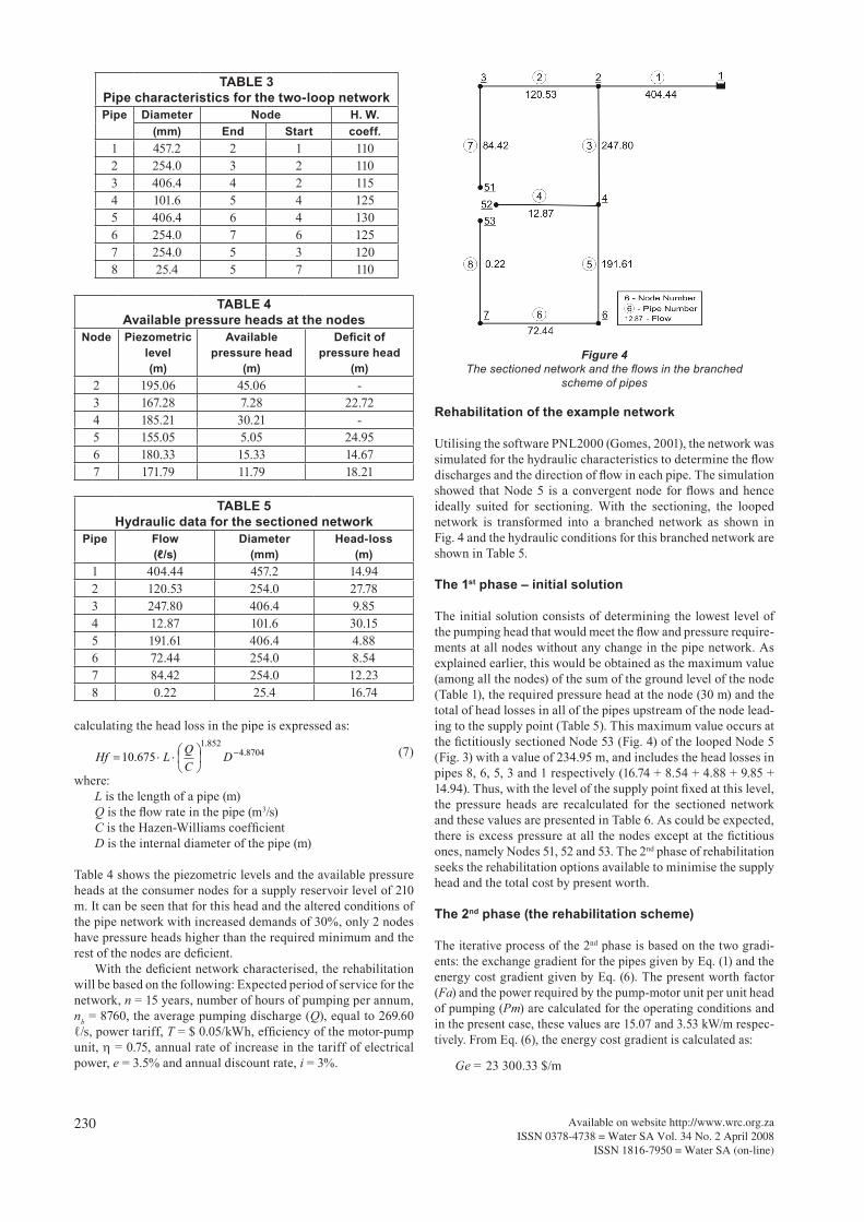
Utilising the software PNL2000 (Gomes, 2001), the network was simulated for the hydraulic characteristics to determine the flow discharges and the direction of flow in each pipe. The simulation showed that Node 5 is a convergent node for flows and hence ideally suited for sectioning. With the sectioning, the looped network is transformed into a branched network as shown in Fig. 4 and the hydraulic conditions for this branched network are shown in Table 5.

The 1st phase – initial solution

The initial solution consists of determining the lowest level of the pumping head that would meet the flow and pressure require-ments at all nodes without any change in the pipe network. As explained earlier, this would be obtained as the maximum value (among all the nodes) of the sum of the ground level of the node (Table 1), the required pressure head at the node (30 m) and the total of head losses in all of the pipes upstream of the node lead-ing to the supply point (Table 5). This maximum value occurs at the fictitiously sectioned Node 53 (Fig. 4) of the looped Node 5 (Fig. 3) with a value of 234.95 m, and includes the head losses in pipes 8, 6, 5, 3 and 1 respectively (16.74 + 8.54 + 4.88 + 9.85 + 14.94). Thus, with the level of the supply point fixed at this level, the pressure heads are recalculated for the sectioned network and these values are presented in Table 6. As could be expected, there is excess pressure at all the nodes except at the fictitious ones, namely Nodes 51, 52 and 53. The 2nd phase of rehabilitation seeks the rehabilitation options available to minimise the supply head and the total cost by present worth.

The 2nd phase (the rehabilitation scheme)

The iterative process of the 2nd phase is based on the two gradi-ents: the exchange gradient for the pipes given by Eq. (1) and the energy cost gradient given by Eq. (6). The present worth factor (Fa) and the power required by the pump-motor unit per unit head of pumping (Pm) are calculated for the operating conditions and in the present case, these values are 15.07 and 3.53 kW/m respec-tively. From Eq. (6), the energy cost gradient is calculated as: Ge = 23 300.33 $/m

TABLE 3Pipe characteristics for the two-loop networkPipe Diameter Node H. W.

(mm) End Start coeff.1 457.2 2 1 1102 254.0 3 2 1103 406.4 4 2 1154 101.6 5 4 1255 406.4 6 4 1306 254.0 7 6 1257 254.0 5 3 1208 25.4 5 7 110

TABLE 4Available pressure heads at the nodes

Node Piezometriclevel(m)

Availablepressure head

(m)

Deficit ofpressure head

(m)2 195.06 45.06 -3 167.28 7.28 22.724 185.21 30.21 -5 155.05 5.05 24.956 180.33 15.33 14.677 171.79 11.79 18.21

8704.4852.1

675.10

DCQLHf

Figure 4

The sectioned network and the flows in the branched scheme of pipes

TABLE 5Hydraulic data for the sectioned network

Pipe Flow(ℓ/s)

Diameter(mm)

Head-loss(m)

1 404.44 457.2 14.942 120.53 254.0 27.783 247.80 406.4 9.854 12.87 101.6 30.155 191.61 406.4 4.886 72.44 254.0 8.547 84.42 254.0 12.238 0.22 25.4 16.74


231

The iterative process

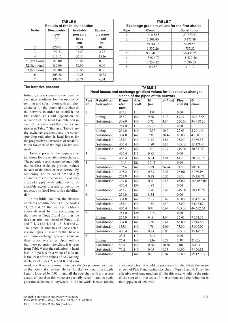
Initially, it is necessary to compare the exchange gradients for the options of relining and substitution with a higher diameter for the potential stretches of the network in order to establish the first choice. This will depend on the reduction of the head loss obtained in each of the cases and these values are shown in Table 7. Shown in Table 8 are the exchange gradients and the corre-sponding reduction in head losses for the progressive alternatives of rehabili-tation for each of the pipes in the net-work. Table 9 presents the sequence of iterations for the rehabilitation choices. The potential sections are the ones with the smallest exchange gradient values in each of the three arteries formed by sectioning. The values of EP and ∆Hf are indicators for the possibility of low-ering of supply heads either due to the available excess pressure or due to the reduction in head loss with rehabilita-tion. In the initial solution, the absence of excess pressure occurs at the Nodes 51, 52 and 53 that are the fictitious nodes derived by the sectioning of the pipes at Node 5 and forming the three arteries composed of Pipes 1, 2 and 7, 1, 3 and 4, and 1, 3, 5, 6 and 8. The potential stretches in these arter-ies are Pipes 2, 4 and 8 that have a minimum exchange gradient value in their respective arteries. Upon analyz-ing these potential stretches, it is seen from Table 9 that the reduction in head loss in Pipe 8 with a value of 6.02 m, is the least of the values of ∆Hf among stretches of Pipes 2, 4 and 8, and also would result in the minimum excess value for pressure upstream of the potential stretches. Hence, for the next trial, the supply head is lowered by 6.02 m and all the stretches with a pressure excess of less than this value are partially rehabilitated to avoid pressure deficiencies anywhere in the network. Hence, for the

TABLE 6 Results of the initial solution

Node Piezometric level (m)

Availablepressure

head(m)

Excess ofpressure

head(m)

2 220.01 70.01 40.013 192.23 32.23 2.234 210.16 55.16 25.16

51 (fictitious) 180.00 30.00 0.0052 (fictitious) 180.00 30.00 0.0053 (fictitious) 180.00 30.00 0.00

6 205.28 40.28 10.287 196.74 36.74 6.74

TABLE 7Exchange gradient values for the first choice

Pipe Cleaning Substitution1 16 315.55 23 870.332 2 201.40 3 175.893 20 361.15 24 199.774 1 332.26 785.325 97 941.16 58 435.256 13 626.77 11 422.567 7 254.32 7 696.338 219.58 410.19

TABLE 8Head losses and exchange gradient values for successive changes

in each of the pipes of the networkPipeNo.

Rehabilita-tion option

Diam-eter (mm)

H. W. coeff.

Hf(m)

∆Hf (m) Pipe cost ($)

G($/m)

1 457.2 110 14.94 - 0.00 -Lining 457.2 140 9.56 5.38 87.79 16 315.55Substitution 508.0 140 5.72 3.84 220.00 34 468.20

2 254.0 110 27.78 - 0.00 -Lining 254.0 140 17.77 10.01 22.03 2 201.40Substitution 304.8 140 7.31 10.46 65.00 4 108.23Substitution 355.6 140 3.45 3.86 75.00 2 589.57Substitution 406.4 140 1.80 1.65 105.00 18 174.44Substitution 457.2 140 1.01 0.79 145.00 50 857.53

3 406.4 115 9.85 - 0.00 -Lining 406.4 140 6.84 3.01 61.26 20 361.15

4 101.6 125 30.13 - 0.00 -Substitution 152.4 140 3.39 26.74 21.00 785.32Substitution 203.2 140 0.83 2.56 28.00 2 739.19Substitution 254.0 140 0.28 0.55 37.00 16 258.78Substitution 304.8 140 0.11 0.17 65.00 168 858.00

5 406.4 130 4.88 - 0.00 -Substitution 457.2 140 2.40 2.48 145.00 58 435.25

6 254.0 125 8.54 - 0.00 -Substitution 304.8 140 2.85 5.69 65.00 11 422.56Substitution 355.6 140 1.35 1.50 75.00 6 648.67Substitution 406.4 140 0.71 0.64 105.00 46 662.64

7 254.0 120 12.23 - 0.00 -Lining 254.0 140 9.19 3.04 22.03 7 254.32Substitution 304.8 140 3.78 5.41 65.00 7 944.50Substitution 355.6 140 1.78 2.00 75.00 5 007.70Substitution 406.4 140 0.93 0.85 105.00 35 145.73

8 25.4 110 17.44 - 0.00 -Lining 25.4 140 11.16 6.28 1.38 219.58Substitution 50.8 140 0.38 10.78 7.00 521.31Substitution 76.2 140 0.05 0.33 10.00 9 126.12Substitution 101.6 140 0.01 0.04 13.00 75 123.53

above reduction, it would be necessary to rehabilitate the entire stretch of Pipe 8 and partial stretches of Pipes 2 and 4. Thus, the effective exchange gradient G*, for this case, would be the ratio of the sum of all the costs of interventions and the reduction in the supply head achieved.



232

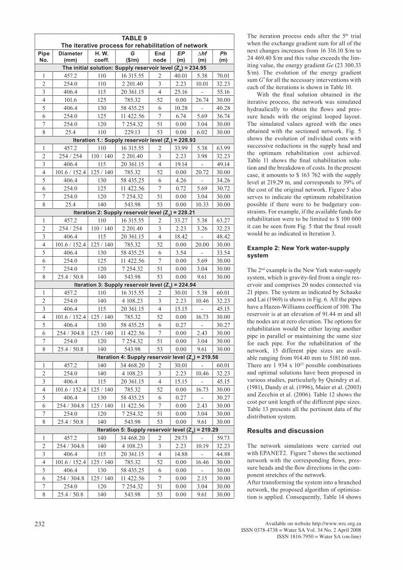
TABLE 9The iterative process for rehabilitation of network

PipeNo.

Diameter (mm)

H. W. coeff.

G($/m)

End node

EP (m)

∆hf (m)

Ph (m)

The initial solution: Supply reservoir level (Z0) = 234.951 457.2 110 16 315.55 2 40.01 5.38 70.012 254.0 110 2 201.40 3 2.23 10.01 32.233 406.4 115 20 361.15 4 25.16 - 55.164 101.6 125 785.32 52 0.00 26.74 30.005 406.4 130 58 435.25 6 10.28 - 40.286 254.0 125 11 422.56 7 6.74 5.69 36.747 254.0 120 7 254.32 51 0.00 3.04 30.008 25.4 110 229.13 53 0.00 6.02 30.00

Iteration 1.: Supply reservoir level (Z1) = 228.931 457.2 110 16 315.55 2 33.99 5.38 63.992 254 / 254 110 / 140 2 201.40 3 2.23 3.98 32.233 406.4 115 20 361.15 4 19.14 - 49.144 101.6 / 152.4 125 / 140 785.32 52 0.00 20.72 30.005 406.4 130 58 435.25 6 4.26 - 34.266 254.0 125 11 422.56 7 0.72 5.69 30.727 254.0 120 7 254.32 51 0.00 3.04 30.008 25.4 140 543.98 53 0.00 10.33 30.00

Iteration 2: Supply reservoir level (Z2) = 228.21 1 457.2 110 16 315.55 2 33.27 5.38 63.272 254 / 254 110 / 140 2 201.40 3 2.23 3.26 32.233 406.4 115 20 361.15 4 18.42 - 48.424 101.6 / 152.4 125 / 140 785.32 52 0.00 20.00 30.005 406.4 130 58 435.25 6 3.54 - 33.546 254.0 125 11 422.56 7 0.00 5.69 30.007 254.0 120 7 254.32 51 0.00 3.04 30.008 25.4 / 50.8 140 543.98 53 0.00 9.61 30.00

Iteration 3: Supply reservoir level (Z3) = 224.94 1 457.2 110 16 315.55 2 30.01 5.38 60.012 254.0 140 4 108.23 3 2.23 10.46 32.233 406.4 115 20 361.15 4 15.15 - 45.154 101.6 / 152.4 125 / 140 785.32 52 0.00 16.73 30.005 406.4 130 58 435.25 6 0.27 - 30.276 254 / 304.8 125 / 140 11 422.56 7 0.00 2.43 30.007 254.0 120 7 254.32 51 0.00 3.04 30.008 25.4 / 50.8 140 543.98 53 0.00 9.61 30.00

Iteration 4: Supply reservoir level (Z4) = 219.56 1 457.2 140 34 468.20 2 30.01 - 60.012 254.0 140 4 108.23 3 2.23 10.46 32.233 406.4 115 20 361.15 4 15.15 - 45.154 101.6 / 152.4 125 / 140 785.32 52 0.00 16.73 30.005 406.4 130 58 435.25 6 0.27 - 30.276 254 / 304.8 125 / 140 11 422.56 7 0.00 2.43 30.007 254.0 120 7 254.32 51 0.00 3.04 30.008 25.4 / 50.8 140 543.98 53 0.00 9.61 30.00

Iteration 5: Supply reservoir level (Z5) = 219.29 1 457.2 140 34 468.20 2 29.73 - 59.732 254 / 304.8 140 4 108.23 3 2.23 10.19 32.233 406.4 115 20 361.15 4 14.88 - 44.884 101.6 / 152.4 125 / 140 785.32 52 0.00 16.46 30.005 406.4 130 58 435.25 6 0.00 - 30.006 254 / 304.8 125 / 140 11 422.56 7 0.00 2.15 30.007 254.0 120 7 254.32 51 0.00 3.04 30.008 25.4 / 50.8 140 543.98 53 0.00 9.61 30.00

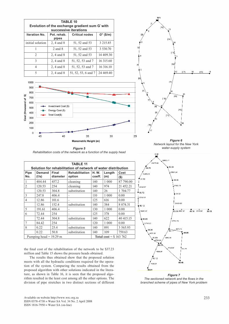
The iteration process ends after the 5th trial when the exchange gradient sum for all of the next changes increases from 16 316.10 $/m to 24 469.40 $/m and this value exceeds the lim-iting value, the energy gradient Ge (23 300.33 $/m). The evolution of the energy gradient sum G* for all the necessary interventions with each of the iterations is shown in Table 10. With the final solution obtained in the iterative process, the network was simulated hydraulically to obtain the flows and pres-sure heads with the original looped layout. The simulated values agreed with the ones obtained with the sectioned network. Fig. 5 shows the evolution of individual costs with successive reductions in the supply head and the optimum rehabilitation cost achieved. Table 11 shows the final rehabilitation solu-tion and the breakdown of costs. In the present case, it amounts to $ 163 762 with the supply level at 219.29 m, and corresponds to 39% of the cost of the original network. Figure 5 also serves to indicate the optimum rehabilitation possible if there were to be budgetary con-straints. For example, if the available funds for rehabilitation were to be limited to $ 100 000 it can be seen from Fig. 5 that the final result would be as indicated in Iteration 3.

Example 2: New York water-supply system

The 2nd example is the New York water-supply system, which is gravity-fed from a single res-ervoir and comprises 20 nodes connected via 21 pipes. The system as indicated by Schaake and Lai (1969) is shown in Fig. 6. All the pipes have a Hazen-Williams coefficient of 100. The reservoir is at an elevation of 91.44 m and all the nodes are at zero elevation. The options for rehabilitation would be either laying another pipe in parallel or maintaining the same size for each pipe. For the rehabilitation of the network, 15 different pipe sizes are avail-able ranging from 914.40 mm to 5181.60 mm. There are 1 934 x 1025 possible combinations and optimal solutions have been proposed in various studies, particularly by Quindry et al. (1981), Dandy et al. (1996), Maier et al. (2003) and Zecchin et al. (2006). Table 12 shows the cost per unit length of the different pipe sizes. Table 13 presents all the pertinent data of the distribution system.

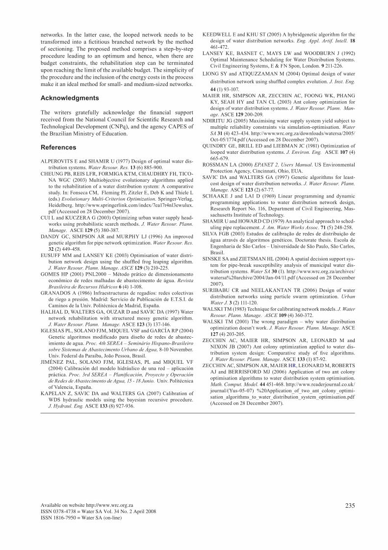
Results and discussion

The network simulations were carried out with EPANET2. Figure 7 shows the sectioned network with the corresponding flows, pres-sure heads and the flow directions in the com-ponent stretches of the network. After transforming the system into a branched network, the proposed algorithm of optimisa-tion is applied. Consequently, Table 14 shows


233

TABLE 10Evolution of the exchange gradient sum G* with

successive iterationsIteration No. Pot. rehab.

pipesCritical nodes G* ($/m)

initial solution 2, 4 and 8 51, 52 and 53 3 215.85

1 2 and 8 51, 52 and 53 3 530.70

2 2, 4 and 8 51, 52 and 53 14 409.30

3 2, 4 and 8 51, 52, 53 and 7 16 315.60

4 2, 4 and 8 51, 52, 53 and 7 16 316.10

5 2, 4 and 8 51, 52, 53, 6 and 7 24 469.40

Figure 5Rehabilitation costs of the network as a function of the supply head

TABLE 11Solution for rehabilitation of network of water distribution

PipeNo.

Demand(ℓ/s)

Finaldiameter

Rehabilitationoption

H. W.coeff.

Length(m)

Cost($)

1 404.44 457.2 cleaning 140 1 000 87 790.002 120.53 254 cleaning 140 974 21 452.21

120.53 304.8 substitution 140 26 1 704.773 247.8 406.4 - 110 1 000 0.004 12.86 101.6 - 125 616 0.00

12.86 152.4 substitution 140 384 8 074.315 191.61 406.4 - 130 1 000 0.006 72.44 254 - 125 378 0.00

72.44 304.8 substitution 140 622 40 415.157 84.42 254 - 120 1 000 0.008 0.22 25.4 substitution 140 891 3 565.93

0.22 50.8 substitution 140 109 759.63 Pumping head = 19.29 m Total cost = $ 163 762

Figure 6Network layout for the New York

water-supply system

Figure 7

The sectioned network and the flows in the branched scheme of pipes of New York problem

the final cost of the rehabilitation of the network to be $37.23 million and Table 15 shows the pressure heads obtained. The results thus obtained show that the proposed solution meets with all the hydraulic conditions required for the opera-tion of the system. Comparing the results obtained from the proposed algorithm with other solutions indicated in the litera-ture, as shown in Table 16, it is seen that the proposed algo-rithm resulted in the least cost among all the other options. The division of pipe stretches in two distinct sections of different



234

diameters is efficient and cost effective, especially when deal-ing with very long stretches of pipes of uniform diameter. For short stretches, however, the practical advantage would be small in using sub-stretches of different sizes and the use of just one diameter for the pipe would be appropriate.

Conclusions

An optimal water-supply pipe network rehabilitation procedure, which is relatively simple, yet takes into account the diverse reha-bilitation options and even the pumping costs, has been demon-strated with an example of its application. The methodology is based on the exchange gradient concept of Granados (1986).

For the rehabilitation of networks considering pipes in paral-lel or substituting the existing ones, using various sizes of pipes in a long stretch results in considerable economy and hence should be considered as a major option in the rehabilitation proc-ess. The methodology presented in this paper is directly applica-ble to branched networks, but could be extended also to looped

TABLE 12Pipe sizes and costs for the New York problem

Diameter (mm) Cost ($/m)914.4 306.76

1 219.2 439.631 524.0 577.431 828.8 725.072 133.6 875.982 438.4 1 036.752 743.2 1 197.513 048.0 1 368.113 352.8 1 538.713 657.6 1 712.603 962.4 1 893.044 267.2 2 073.494 572.0 2 260.504 876.8 2 447.515 181.6 2 637.80

TABLE 13Network data for the New York water-supply system

Link data Node dataPipeNo.

Existing diameter

(mm)

Length(m)

NodeNo.

Demand(ℓ/s)

Minimumhead (m)

[1] 4 572.0 3 535.68 1 Reservoir -[2] 4 572.0 6 035.04 2 2 616.477 77.724[3] 4 572.0 2 225.04 3 2 616.477 77.724[4] 4 572.0 2 529.84 4 2 497.546 77.724[5] 4 572.0 2 621.28 5 2 497.546 77.724[6] 4 572.0 5 821.68 6 2 497.546 77.724[7] 3 352.8 2 926.08 7 2 497.546 77.724[8] 3 352.8 3 810.00 8 2 497.546 77.724[9] 4 572.0 2 926.08 9 4 813.864 77.724[10] 5 181.6 3 413.76 10 28.317 77.724[11] 5 181.6 4 419.60 11 4 813.864 77.724[12] 5 181.6 3 718.56 12 3 315.903 77.724[13] 5 181.6 7 345.68 13 3 315.903 77.724[14] 5 181.6 6 431.28 14 2 616.477 77.724[15] 5 181.6 4 724.40 15 2 616.477 77.724[16] 1 828.8 8 046.72 16 4 813.864 79.248[17] 1 828.8 9 509.76 17 1 628.219 83.149[18] 1 524.0 7 315.20 18 3 315.903 77.724[19] 1 524.0 4 389.12 19 3 315.903 77.724[20] 1 524.0 11 704.32 20 4 813.864 77.724[21] 1 828.8 8 046.72

TABLE 14Optimised solution for rehabilitation of the

New York networkPipeNo.

Diameter(mm)

Length(m)

Cost($)

7 1 828.8 37.14 26 929.101 524.0 2 888.94 1 668 160.62

16 2 743.2 8 046.72 9 636 027.6717 2 743.2 1 870.10 2 239 463.45

2 438.4 7 639.66 7 920 417.5118 2 133.6 7 315.20 6 407 968.9019 1 524.0 4 257.63 2 458 483.29

1 219.2 131.49 57 806.9521 2 133.6 6 299.87 5 693 756.12

1 828.8 1 746.85 1 121 574.53 Total cost = 37 230 588.13

TABLE 15The final pressure heads at the nodes of the New York network

Node No. Pressure head (m)2 89.7463 87.4014 86.7185 86.1186 85.6577 84.9418 84.1019 83.33910 83.28511 83.44212 83.74713 83.64014 86.89215 89.34016 79.20917 83.10718 79.74719 77.87920 78.351

TABLE 16Cost comparisons of solutions proposed in the

literature for the New York networkAuthor Cost

($ million)Schaake and Lai (1969) 78.09Quindry et al. (1981) 63.58Dandy et al. (1996) 38.80Maier et al. (2003) 38.64Zecchin et al. (2006) 38.64Present study (based on Granado’s method) 37.23


235

networks. In the latter case, the looped network needs to be transformed into a fictitious branched network by the method of sectioning. The proposed method comprises a step-by-step procedure leading to an optimum and hence, when there are budget constraints, the rehabilitation step can be terminated upon reaching the limit of the available budget. The simplicity of the procedure and the inclusion of the energy costs in the process make it an ideal method for small- and medium-sized networks.

Acknowledgments

The writers gratefully acknowledge the financial support received from the National Council for Scientific Research and Technological Development (CNPq), and the agency CAPES of the Brazilian Ministry of Education.

References

ALPEROVITS E and SHAMIR U (1977) Design of optimal water dis-tribution systems. Water Resour. Res. 13 (6) 885-900.

CHEUNG PB, REIS LFR, FORMIGA KTM, CHAUDHRY FH, TICO- NA WGC (2003) Multiobjective evolutionary algorithms applied to the rehabilitation of a water distribution system: A comparative study. In: Fonseca CM, Fleming PJ, Zitzler E, Deb K and Thiele L (eds.) Evolutionary Multi-Criterion Optimization. Springer-Verlag, Heidelberg. http://www.springerlink.com/index/7ea17r4nl3ewulux.pdf (Accessed on 28 December 2007).

CUI L and KUCZERA G (2003) Optimizing urban water supply head-works using probabilistic search methods. J. Water Resour. Plann. Manage. ASCE 129 (5) 380-387.

DANDY GC, SIMPSON AR and MURPHY LJ (1996) An improved genetic algorithm for pipe network optimization. Water Resour. Res. 32 (2) 449-458.

EUSUFF MM and LANSEY KE (2003) Optimisation of water distri-bution network design using the shuffled frog leaping algorithm. J. Water Resour. Plann. Manage. ASCE 129 (3) 210-225.

GOMES HP (2001) PNL2000 – Método prático de dimensionamento econômico de redes malhadas de abastecimento de água. Revista Brasileira de Recursos Hídricos 6 (4) 1-108.

GRANADOS A (1986) Infraestructuras de regadíos: redes colectivas de riego a presión. Madrid: Servicio de Publicación de E.T.S.I. de Caminos de la Univ. Politécnica de Madrid, España.

HALHAL D, WALTERS GA, OUZAR D and SAVIC DA (1997) Water network rehabilitation with structured messy genetic algorithm. J. Water Resour. Plann. Manage. ASCE 123 (3) 137-146.

IGLESIAS PL, SOLANO FJM, MIQUEL VSF and GARCÍA RP (2004) Genetic algoritmos modificado para diseño de redes de abastec-imiento de agua. Proc. 4th SEREA – Seminário Hispano-Brasileiro sobre Sistemas de Abastecimento Urbano de Água, 8-10 November. Univ. Federal da Paraíba, João Pessoa, Brasil.

JIMÉNEZ PAL, SOLANO FJM, IGLESIAS, PL and MIQUEL VF (2004) Calibración del modelo hidráulico de una red – aplicación práctica. Proc. 3rd SEREA – Planificación, Proyecto y Operación de Redes de Abastecimento de Agua, 15 - 18 Junio. Univ. Politécnica of Valencia, España.

KAPELAN Z, SAVIC DA and WALTERS GA (2007) Calibration of WDS hydraulic models using the bayesian recursive procedure. J. Hydraul. Eng. ASCE 133 (8) 927-936.

KEEDWELL E and KHU ST (2005) A hybridgenetic algorithm for the design of water distribution networks. Eng. Appl. Artif. Intell. 18 461-472.

LANSEY KE, BASNET C, MAYS LW and WOODBURN J (1992) Optimal Maintenance Scheduling for Water Distribution Systems. Civil Engineering Systems, E & FN Spon, London. 9 211-226.

LIONG SY and ATIQUZZAMAN M (2004) Optimal design of water distribution network using shuffled complex evolution. J. Inst. Eng. 44 (1) 93-107.

MAIER HR, SIMPSON AR, ZECCHIN AC, FOONG WK, PHANG KY, SEAH HY and TAN CL (2003) Ant colony optimization for design of water distribution systems. J. Water Resour. Plann. Man-age. ASCE 129 200-209.

NDIRITU JG (2005) Maximising water supply system yield subject to multiple reliability constraints via simulation-optimisation. Water SA 31 (4) 423-434. http://www.wrc.org.za/downloads/watersa/2005/Oct-05/1774.pdf (Accessed on 28 December 2007).

QUINDRY GE, BRILL ED and LIEBMAN JC (1981) Optimization of looped water distribution systems. J. Environ. Eng. ASCE 107 (4) 665-679.

ROSSMAN LA (2000) EPANET 2, Users Manual. US Environmental Protection Agency, Cincinnati, Ohio, EUA.

SAVIC DA and WALTERS GA (1997) Genetic algorithms for least-cost design of water distribution networks. J. Water Resour. Plann. Manage. ASCE 123 (2) 67-77.

SCHAAKE J and LAI D (1969) Linear programming and dynamic programming applications to water distribution network design, Research Report No. 116, Department of Civil Engineering, Mas-sachusetts Institute of Technology.

SHAMIR U and HOWARD CD (1979) An analytical approach to sched-uling pipe replacement. J. Am. Water Works Assoc. 71 (5) 248-258.

SILVA FGB (2003) Estudos de calibração de redes de distribuição de água através de algoritmos genéticos. Doctorate thesis. Escola de Engenharia de São Carlos – Universidade de São Paulo, São Carlos, Brasil.

SINSKE SA and ZIETSMAN HL (2004) A spatial decision support sys-tem for pipe-break susceptibility analysis of municipal water dis-tribution systems. Water SA 30 (1). http://www.wrc.org.za/archives/watersa%20archive/2004/Jan-04/11.pdf (Accessed on 28 December 2007).

SURIBABU CR and NEELAKANTAN TR (2006) Design of water distribution networks using particle swarm optimization. Urban Water J. 3 (2) 111-120.

WALSKI TM (1983) Technique for calibrating network models. J. Water Resour. Plann. Manage. ASCE 109 (4) 360-372.

WALSKI TM (2001) The wrong paradigm – why water distribution optimization doesn’t work. J. Water Resour. Plann. Manage. ASCE 127 (4) 203-205.

ZECCHIN AC, MAIER HR, SIMPSON AR, LEONARD M and NIXON JB (2007) Ant colony optimization applied to water dis-tribution system design: Comparative study of five algorithms. J. Water Resour. Plann. Manage. ASCE 133 (1) 87-92.

ZECCHIN AC, SIMPSON AR, MAIER HR, LEONARD M, ROBERTS AJ and BERRISFORD MJ (2006) Application of two ant colony optimisation algorithms to water distribution system optimisation. Math. Comput. Model. 44 451-468. http://www.readerjournal.co.uk/journal/(Yus-05-07) %20Application_of_two_ant_colony_optimi-sation_algorithms_to_water_distribution_system_optimisation.pdf (Accessed on 28 December 2007).

http://www.springerlink.com/index/7ea17r4nl3ewulux.pdf

http://www.springerlink.com/index/7ea17r4nl3ewulux.pdf

http://www.wrc.org.za/downloads/watersa/2005/Oct-05/1774.pdf

http://www.wrc.org.za/downloads/watersa/2005/Oct-05/1774.pdf

http://www.wrc.org.za/archives/watersa archive/2004/Jan-04/11.pdf

http://www.wrc.org.za/archives/watersa archive/2004/Jan-04/11.pdf

http://www.readerjournal.co.uk/journal/(Yus-05-07) Application_of_two_ant_colony_optimisation_algorithms_to_water_distribution_system_optimisation.pdf





236

Documents

An iterative optimisation procedure for the rehabilitation