l The New York Fed’s Survey of Consumer Expectations (SCE) gathers information on consumer expectations regarding inflation, household finance, the labor and housing markets, and other economic issues.

l Launched in 2013 and fielded monthly, the survey aims to help researchers and policymakers understand how expectations are formed and how they affect consumer behavior—behavior that, in aggregate, helps drive macroeconomic activity and hence has implications for monetary policy.

l This article explores the survey’s history, format, and question construction; details the procedure for selecting the rotating panel of survey participants; and describes the methods used to calculate statistics and disseminate results.

l The authors also outline the benefits of soliciting “density forecasts,” which measure uncertainty, in addition to simple “point forecasts,” and explain the rationale for seeking expectations on “inflation” rather than “prices.”

FRBNY Economic Policy Review / December 2017 51

1. Introduction

The importance of compiling high-quality data on the expectations held by economic agents has been increasingly recognized in both academic research and policymaking. Most economic decisions involve uncertainty and should therefore take into account not only preferences but also expectations about the future. Expectations should drive a variety of economic choices made by households, including those related to saving, investment, purchases of durable goods, wage negotiations, and so on. The aggregation of these choices in turn determines macroeconomic outcomes, including realized inflation, in equilibrium. Given the role of households in aggregate as an important driver of economic activity, the monitoring and management of consumers’ expectations have become primary goals of policymakers and central components of modern monetary policy (Woodford 2004; Bernanke 2007; Gali 2008; Sims 2009).1

The effectiveness of monetary policy and central bank communication relies on longer-run inflation expectations being well-anchored, making the measurement of these expectations important for policymakers. More generally, consumers’ expectations about a number of personal and

1 In particular, Bernanke (2004) argued that “an essential prerequisite to controlling inflation is to control inflation expectations.”

Olivier Armantier, Giorgio Topa, Wilbert van der Klaauw, and Basit Zafar

An Overview of the Survey of Consumer Expectations

Olivier Armantier is an assistant vice president, Giorgio Topa a vice president, Wilbert van der Klaauw a senior vice president, and Basit Zafar a former research officer at the Federal Reserve Bank of New York.

olivier.armantier@ny.frb.orggiorgio.topa@ny.frb.orgwilbert.vanderklaauw@ny.frb.orgbasit.zafar@asu.edu

The views expressed in this article are those of the authors and do not necessarily reflect the position of the Federal Reserve Bank of New York or the Federal Reserve System.

To view the authors’ disclosure statements, visit https://www.newyorkfed.org/research/author_disclosure/ad_epr_2017_overview-of-sce_armantier.

52 An Overview of the Survey of Consumer Expectations

macroeconomic outcomes are increasingly useful inputs into a variety of forecasting models.

Effective monitoring and management of expectations requires the measurement of consumer expectations and an understanding of how these expectations are formed. The Federal Reserve Bank of New York’s Survey of Consumer Expectations (SCE) was developed with precisely these goals in mind. The SCE collects timely, high-frequency information about consumer expectations and decisions on a broad variety of topics. Its overall goal is to fill the gaps in existing data sources (such as the University of Michigan Survey of Consumers, the Federal Reserve Board’s Survey of Consumer Finances, and the Bureau of Labor Statistics’ Consumer Expenditure Survey) pertaining to household expectations and behavior by providing a more integrated data approach. The SCE aims to cover a broad range of economic outcomes, including infla-tion, household finance, the labor market, and the housing market, as well as special topics as the need arises for policy or research analysis.2

The SCE is designed as a rotating panel, which enables researchers and policymakers to follow the same individu-als over time, reducing changes in the sample’s composition and thus minimizing sampling volatility in survey responses from month to month. The panel structure of the SCE is designed to provide valuable input into the evaluation of the economic outlook and policy formulation, and to offer an important resource for the research community to both increase its understanding of how consumers form and update their expectations and better assess the links between expectations and behavior. For instance, the data allow one to study how expectations about house prices and interest rates affect consumers’ choices regarding buying or renting a home or regarding the type of mort-gage used to purchase a home. Data on expectations about the likelihood of finding a job and about future wage earnings may be used to analyze workers’ job search behav-ior or retirement decisions. Researchers may also study how inflation expectations shape consumers’ spending

2 National surveys of public (inflation) expectations are now conducted in multiple countries. In the United States, these include the University of Michigan Survey of Consumers, the Livingston Survey, the Conference Board’s Consumer Confidence Survey, and the Survey of Professional Forecasters. Other central banks that survey consumers about their inflation expectations include the Bank of England, the European Central Bank, the Bank of Japan, the Reserve Bank of India, and the Sveriges Riksbank. Since 2015, the Bank of Canada has conducted a largely comparable version of the SCE, fielded at a quarterly frequency. Since 2013, the Federal Reserve Board has conducted the Survey of Household Economics and Decisionmaking (SHED), which elicits some expectations about the economic well-being of U.S. households.

and saving behavior. Collecting such data for the same households over time enables researchers to study potential interactions between decisions and expectations across many different domains of consumer behavior. Finally, the data can be used to study the evolution of a diverse but related set of expectations and the way they co-vary over time at the individual level, and to identify any (structural) breaks in this relationship.

A key feature of the SCE is its reliance on a probabilistic question format to elicit the likelihood respondents assign to different future events. In addition to questions asking respondents for point forecasts—for example, in the case of year-ahead inflation, What do you expect the rate of [inflation/deflation] to be over the next twelve months?—for several continuous outcomes, we ask for density fore-casts—that is, the percent chance the respondent assigns to different future possible values of that variable. In the case of future inflation, for example, respondents are asked for the likelihood that future inflation will fall within different prespecified intervals. These density forecasts allow respondents to express uncertainty regarding their expectations. For binary outcomes (where the event either occurs or does not occur), eliciting the percent chance associated with the event fully identifies the underlying subjective distribution. By obtaining density forecasts, the SCE extends a practice with a longer tradition in the field of psychology and in surveys of professional forecasters, economists, and other financial experts. Our approach also builds on a large and growing body of economic research, led by Charles Manski, that has demonstrated survey respondents’ willingness and ability to answer questions expressed in this way.

Finally, the SCE is conducted as a monthly internet survey in order to provide more flexibility in terms of question design and more real-time capabilities for data collection. An internet platform enables the researcher to design more user-friendly questions, with the help of visual aids and other tools that make it easier for respondents to understand and answer a specific question. An internet platform also makes it easier to develop and field new questions on special topics at short notice. For example, we designed and fielded special surveys to help assess how consumers’ spending and inflation expectations responded to sudden large declines in gas prices and to elicit beliefs regarding the early impact of the Affordable Care Act on future healthcare spending, prices, and coverage.

FRBNY Economic Policy Review / December 2017 53

1.1 Survey Overview

The SCE started in June 2013, after a six-month initial testing phase.3 It is a nationally representative, internet-based survey of a rotating panel of about 1,300 household heads, where household head is defined as the person in the household who owns, is buying, or rents the home. The survey is con-ducted monthly. New respondents are drawn each month to match various demographic targets from the American Community Survey (ACS), and they stay on the panel for up to twelve months before rotating out. The survey instrument is fielded on an internet platform designed by the Demand Institute, a nonprofit organization jointly oper-ated by the Conference Board and Nielsen. The respondents for the SCE come from the sample of respondents to the Consumer Confidence Survey (CCS), a mail survey conducted by the Conference Board. In turn, the respondents for the CCS are selected from the universe of U.S. Postal Service addresses. From that universe, a new random sample is drawn each month, stratified only by Census division.

The SCE has several components. First, it includes a core monthly module on expectations about a number of macroeconomic and household-level variables.4 In this module, respondents are asked about their inflation expecta-tions, as well as their expectations regarding changes in home prices and the prices of various specific spending items, such as gasoline, food, rent, medical care, and college education. The core survey also asks for expectations about unemploy-ment, interest rates, the stock market, credit availability, taxes, and government debt. In addition, respondents are asked to report their expectations about several labor market outcomes that pertain to them, including changes in their earnings, the perceived probability of losing their current job (or leaving their job voluntarily), and the perceived probability of finding a job. Finally, the core survey asks about the expected change in respondent households’ overall income and spending. As described in more detail below, these questions about expec-tations are fielded at various time horizons and with various formats, including both point and density forecasts.

Second, each month, the SCE contains a supplementary “ad hoc” module on special topics. Three such modules are repeated every four months, leaving three “floating” supplements per year on topics that are determined as the

3 As discussed below, the SCE was preceded by an extensive feasibility study over the period 2006-13, using experimental surveys on the RAND Corporation’s American Life Panel. Early findings from that study are described in van der Klaauw et al. (2008). 4 Each entering cohort is also administered a module with demographic questions about the respondent and the respondent’s household.

need arises. The three repeating supplements are on credit access, labor market, and spending. Topics covered so far in the “floating” supplement include (but are not limited to) the Affordable Care Act, student loans, workplace benefits such as childcare and family leave, and the use of insurance products. Together, the core monthly module and the monthly supple-ment take about fifteen minutes to complete.

Finally, SCE respondents also fill out longer surveys (up to thirty minutes in length, and separate from the monthly survey) each quarter on various topics. Most of these surveys are repeated at a yearly frequency. Since each SCE panelist stays in the panel for up to twelve months, these annual surveys can be used as independent repeated cross sections, although they obviously can be linked to the monthly core survey panel responses. The SCE currently contains quarterly surveys on the housing market, the labor market, informal work participation, and consumption, saving, and assets. A subset of these surveys is designed in part or wholly by other Federal Reserve Banks.

2. Questionnaire Design

The 1990s represented a period of significant change in the way economists elicit expectations through surveys. Tradi-tionally, researchers have measured expectations through verbal and qualitative questions, asking respondents whether they expect that an event will occur or not, or asking whether they think it is “very likely,” “fairly likely,” “not too likely,” or “not at all likely” that a specific event will occur. In addition to the limited information captured owing to the coarseness of choice options or to the lack of means for expressing uncertainty altogether, a major drawback of this traditional approach concerns the lack of inter- and intrapersonal compa-rability of responses.

Led and inspired by the work of Charles Manski, who in turn built on the early work of Juster (1966) and a longer tradition of collecting such data in cognitive psychology, economists began to elicit probabilistic expectations during the 1990s. It quickly became clear that, with some guidance, survey respondents are able and willing to answer probabilis-tic expectations questions.5 Moreover, with a fixed numerical scale, responses are interpersonally comparable and have been found to be better predictors of outcomes. A growing number of large-scale surveys in the United States and abroad now use probabilistic formats to elicit expectations for a wide

5 Usually before such questions are asked, respondents are provided with a brief introduction or explanation of basic probabilistic ideas through examples.

54 An Overview of the Survey of Consumer Expectations

range of events, and these formats have also been successfully implemented in surveys associated with laboratory and field experiments, including several conducted in less developed countries. Manski (2004) reviews research eliciting proba-bilistic expectations in surveys and assesses the state of the art at that time. Delavande (2014) and Delavande, Giné, and McKenzie (2011) provide a more recent review.

The questionnaire design of the SCE builds on this previous research and was informed, in large part, by our experiences with the Household Inflation Expectations Project (HIEP), wherein we fielded surveys every six weeks on RAND’s American Life Panel (ALP) going back to 2007 (Bruine de Bruin et al. 2010a). The HIEP questionnaires were developed in collaboration with RAND, other Federal Reserve Banks, academic economists, psychologists, and survey design experts. During the period 2006 to 2012, the HIEP conducted in-depth cognitive interviews, fielded psychometric surveys on the ALP as well as on various “convenience” (that is, nonrandom) samples, and administered a number of exper-imental consumer surveys in the ALP. In addition to testing probabilistic question formats, we also experimented with alternative wording of questions, especially those related to inflation (discussed in more detail below). The findings from this project formed the basis for the creation of the SCE (see van der Klaauw et al. 2008; Armantier et al. 2013).

During the SCE’s experimental or development phase, between December 2012 and June 2013, we further sharpened and tested the questionnaire. The process involved conducting additional cognitive interviews with a small auxiliary sample to identify potential interpretations of the questions. After inter-viewees read the questions out loud, they were instructed to think out loud while generating their answers. This step allowed us to gauge whether, in fact, interviewees interpreted the ques-tions the way we had intended them to. When necessary, we modified the wording of questions accordingly. Pilot surveys were also conducted and we analyzed the resulting data to make sure the questions were eliciting meaningful variation.

Of particular importance were our findings in the SCE questionnaire development phase regarding the elicitation of expectations. In both the HIEP and the SCE experimen-tal phase, we tested a large set of probabilistic questions. Respondents in our surveys showed a consistent ability and willingness to assign a probability (or “percent chance”) to future events. Unlike simple point forecasts, probabilistic expectations of binary outcomes as well as density forecasts for continuous outcomes provide a valuable measure of individual uncertainty. Moreover, we found these responses to be largely internally consistent in terms of simple laws of probabilities. Finally, we conducted an experiment that confirmed that the densities elicited were informative

(Armantier et al. 2013). For a review of this work, see van der Klaauw et al. (2008) and Bruine de Bruin et al. (2010a, 2011).

Having discussed the SCE questionnaire development process, we now turn to the actual questions, focusing on the SCE core survey. The quantitative questions can be broadly divided into three categories: (1) questions that elicit expectations of binary outcomes (such as the likelihood that the U.S. stock market will be higher in twelve months), (2) questions that elicit pointwise expecta-tions for continuous outcomes (such as the rate of inflation over the next twelve months), and (3) questions that elicit respondents’ probability densities for forecasts of continuous outcomes. Besides these questions, the survey also includes some qualitative questions, including those in which respondents are asked to answer using a (for example) seven-point rating scale. The full questionnaire is available on the New York Fed’s website.6

The bulk of the survey elicits near-term expectations, that is, expectations regarding outcomes over the next twelve months, the next three months, or both. The ad hoc supplements also contain questions at the four-month horizon. However, in certain instances, such as inflation or home prices, expectations are also elicited for the medium term—that is, three years out.

We next describe the rationale for how we elicit some of these expectations.

2.1 Eliciting Expectations of Continuous Outcomes

For some continuous outcomes, we elicit both point and density forecasts. We begin here by illustrating the format of our point forecast questions, and we describe the density forecast questions in Section 2.3.

Inflation Expectations

Inflation expectations are elicited using the following two- stage format. Respondents are first asked: Over the next twelve months, do you think that there will be inflation or deflation? (Note: Deflation is the opposite of inflation).

6 https://www.newyorkfed.org/medialibrary/interactives/sce/sce/downloads/data/FRBNY-SCE-Survey-Core-Module-Public-Questionnaire.pdf.

FRBNY Economic Policy Review / December 2017 55

Depending on their answer to this question, respondents are next asked for a point estimate: What do you expect the rate of [inflation/deflation] to be over the next twelve months? Please give your best guess.

Note that we directly ask respondents for the rate of “inflation.” This differs from the widely used approach of avoiding the term “inflation” in consumer surveys. Most existing inflation expectations questions, such as those posed in the Michigan Survey (Curtin 2006), ask for expected changes in “prices” as follows: During the next twelve months, do you think that prices in general will go up, or go down, or stay where they are now?, with the response options “Go up,” “Stay the same,” and “Go down.” Those who respond “go up” or “go down” are then asked to give a specific point estimate.

We prefer asking respondents for their expectations about “inflation” because our prior research in the HIEP suggests that the way the Michigan Survey question is phrased induces mixed interpretations, with some respondents thinking about specific prices they pay and others thinking about the overall rate of inflation. As the former tend to think more of salient price changes, they are more likely to provide extreme responses (Bruine de Bruin, van der Klaauw, and Topa 2011). We found that asking directly about the rate of inflation reduces ambiguity in interpreting questions, and yields, we believe, more reliable, more interpersonally comparable responses. Moreover, this approach is consistent with the concept of forward inflation expectations, which are of inter-est to central banks.

One source of hesitation in asking consumers about inflation may be the concern that inflation is a relatively complex concept. However, evidence suggests that consumers tend to have a basic understanding of what the term means (Leiser and Drori 2005; Svenson and Nilsson 1986). Cognitive interviews conducted during the HIEP similarly indicate that the vast majority of consumers have a good understanding of the concept of inflation (van der Klaauw et al. 2008; Bruine de Bruin et al. 2012). Furthermore, our research indicates that consumers act on their reported inflation expectations in sensible ways (Armantier et al. 2015) and that they update their inflation expectations meaningfully when provided with arguably inflation-relevant information (Armantier et al. 2016).

In addition, during the period May 2013 to September 2015, we asked SCE survey respondents the following question: On a scale of 1 to 7, how well would you say you understand what “inflation” means? (where 1 means “I don’t know what ‘inflation’ means,” and 7 is labeled as “I know exactly what ‘inflation’ means”). Of the 5,182 first-time respondents to whom this question was posed, only 44 (less than 0.9 percent) chose 1 (no understanding) on the scale. In fact, 82 percent

of respondents chose 5 or higher, suggesting that inflation is a fairly well-understood concept. This, of course, does not mean that households find it easy to express inflation in quantitative terms. To investigate this, we asked our survey respondents the following: On a scale of 1 to 7, how easy is it for you to express the rate of inflation as a number? (where 1 is “Very easy” and 7 is “Very difficult”). Of the 5,179 respondents, 82 percent reported 5 or lower, with just 5.6 percent choosing 7 on the scale. Overall, these results offer convincing evidence that the vast majority of consumers understand the concept of infla-tion and are able to express it numerically.

Expectations for Other Continuous Outcomes

We next present the wording for one other representative set of questions, pertaining to earnings expectations for those who are employed. Respondents are asked:

Please think ahead to twelve months from now. Suppose that you are working in the exact same job at the same place you currently work, and working the exact same number of hours. What do you expect to have happened to your earnings on this job, before taxes and deductions?

○ increase by 0 percent or more ○ decrease by 0 percent or more

This first part is then followed by: By about what percent do you expect your earnings to have [increased/decreased]?

Note that respondents are not presented with a “stay the same” option in the first part of the question. Instead, the instructions specify that they can enter a zero change by picking either the increase or the decrease option and then entering zero in the second part of the question. When experimenting with the wording of questions, we found that a substantial proportion of respondents would choose “stay the same” when that option was available. Upon questioning respondents further, we found that a substantial proportion of those who had chosen “stay the same” had changes in mind that were bigger than 0.5 percent in mag-nitude, suggesting that the mere availability of the “stay the same” option was leading some respondents to select it. In our analysis, we found that the distribution of responses to a given question with and without the “stay the same” option was noticeably different. More research is clearly

56 An Overview of the Survey of Consumer Expectations

needed to understand which elicitation method is best at recovering the true underlying subjective belief. However, given that respondents can always enter zero and hence we arguably elicit more information without the “stay the same” option, we chose to ask for changes without the “stay the same” option.

In addition to the questions we just discussed that ask for point forecasts for inflation and earnings, we use this same question format for a wide range of other outcomes.

2.2 Eliciting Expectations of Binary Outcomes

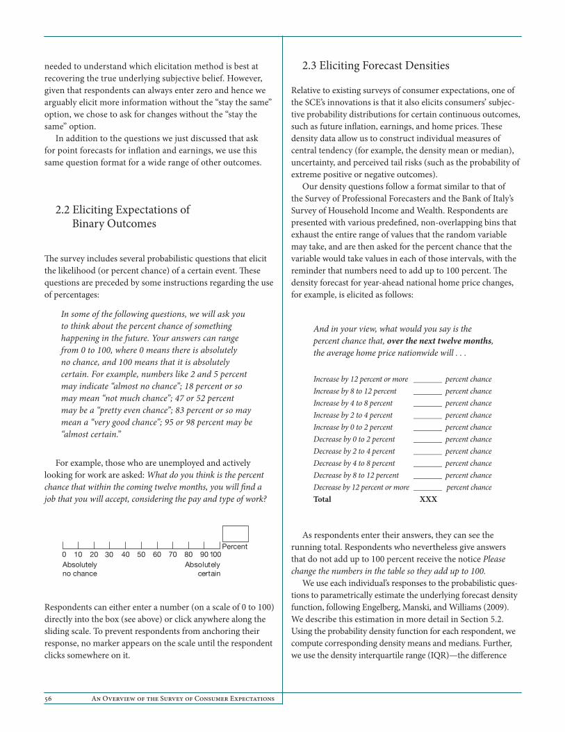
The survey includes several probabilistic questions that elicit the likelihood (or percent chance) of a certain event. These questions are preceded by some instructions regarding the use of percentages:

In some of the following questions, we will ask you to think about the percent chance of something happening in the future. Your answers can range from 0 to 100, where 0 means there is absolutely no chance, and 100 means that it is absolutely certain. For example, numbers like 2 and 5 percent may indicate “almost no chance”; 18 percent or so may mean “not much chance”; 47 or 52 percent may be a “pretty even chance”; 83 percent or so may mean a “very good chance”; 95 or 98 percent may be “almost certain.”

For example, those who are unemployed and actively looking for work are asked: What do you think is the percent chance that within the coming twelve months, you will find a job that you will accept, considering the pay and type of work?

Respondents can either enter a number (on a scale of 0 to 100) directly into the box (see above) or click anywhere along the sliding scale. To prevent respondents from anchoring their response, no marker appears on the scale until the respondent clicks somewhere on it.

2.3 Eliciting Forecast Densities

Relative to existing surveys of consumer expectations, one of the SCE’s innovations is that it also elicits consumers’ subjec-tive probability distributions for certain continuous outcomes, such as future inflation, earnings, and home prices. These density data allow us to construct individual measures of central tendency (for example, the density mean or median), uncertainty, and perceived tail risks (such as the probability of extreme positive or negative outcomes).

Our density questions follow a format similar to that of the Survey of Professional Forecasters and the Bank of Italy’s Survey of Household Income and Wealth. Respondents are presented with various predefined, non-overlapping bins that exhaust the entire range of values that the random variable may take, and are then asked for the percent chance that the variable would take values in each of those intervals, with the reminder that numbers need to add up to 100 percent. The density forecast for year-ahead national home price changes, for example, is elicited as follows:

And in your view, what would you say is the percent chance that, over the next twelve months, the average home price nationwide will . . .

Increase by 12 percent or more _______ percent chanceIncrease by 8 to 12 percent _______ percent chanceIncrease by 4 to 8 percent _______ percent chanceIncrease by 2 to 4 percent _______ percent chanceIncrease by 0 to 2 percent _______ percent chanceDecrease by 0 to 2 percent _______ percent chanceDecrease by 2 to 4 percent _______ percent chanceDecrease by 4 to 8 percent _______ percent chanceDecrease by 8 to 12 percent _______ percent chanceDecrease by 12 percent or more _______ percent chanceTotal XXX

As respondents enter their answers, they can see the running total. Respondents who nevertheless give answers that do not add up to 100 percent receive the notice Please change the numbers in the table so they add up to 100.

We use each individual’s responses to the probabilistic ques-tions to parametrically estimate the underlying forecast density function, following Engelberg, Manski, and Williams (2009). We describe this estimation in more detail in Section 5.2. Using the probability density function for each respondent, we compute corresponding density means and medians. Further, we use the density interquartile range (IQR)—the difference

0 100908070605040302010Absolutely no chance

Absolutely certain

Percent

FRBNY Economic Policy Review / December 2017 57

between the third and the first quartiles—as a measure of indi-vidual forecast uncertainty. We choose this measure because the IQR is less sensitive than, say, the standard deviation to small variations in the tails of the estimated density.

3. Implementation

3.1 Sample Design

The SCE sample design is based on that of the Conference Board’s monthly Consumer Confidence Survey (CCS). The CCS is a mail survey that uses an address-based probability sample design to select a new random sample each month based on the universe of U.S. Postal Service addresses.7 The universe of addresses is derived from the files created by the U.S. Postal Service and represents near-universal coverage of all residential households in the United States.It is updated monthly to ensure up-to-date coverage of U.S. households. The targeted responding CCS sample size is approximately 3,000 completed questionnaires each month from household heads. Questionnaire instructions define household head as the person in your household who owns, is buying, or rents this home.8

The SCE sampling frame (or sampling population) consists of CCS respondents who expressed an ability and a willing-ness to participate in the SCE based on their answers to two questions included at the end of the CCS questionnaire. The first asks: Do you have access to the internet and an email address? Those who answer “Yes” are then asked:

You may be eligible to participate in a survey about your perceptions of the economy, employment, finances, and related topics. This is a paid survey that would be conducted monthly for up to twelve months.

7 The CCS random sample of household addresses is drawn after first stratifying geographically by nine Census divisions to provide a proportionate geographic distribution. To ensure proportional representation in the sample of respond-ents, the CCS uses weights based on gender, income, geography, and age.8 This definition is similar to that used in the Current Population Survey, in the ACS, and by the Census more generally: there, the “reference person” in the household (or the “householder”) is the person who owns or rents the unit of residence. Note that the instructions state that if that person is not available or is unable, an adult aged eighteen or older who lives in the household should complete the survey. In a representative month (March 2013), 96 percent (95 percent weighted) of CCS respondents were household heads, with very little variation across gender, age, income, and race/ethnicity. Note also that this definition does not exclude the possibility that a household may have multiple “co-household heads.”

You would receive $15 for each completed survey.9 If selected, we would email you a web address where you could respond to the online questionnaire.Would you be interested in participating in this monthly, paid survey?

Yes, my email address is:__________________________No, I am not interested in participating

As discussed in more detail below, on average, 53 percent of CCS respondents in a given month express a willingness to participate in a new online survey.10 Of those who are inter-ested in participating, approximately 300 to 320 are invited within the following two months to join the SCE internet panel, of whom about 150 to 180 actually end up joining. A stratified random sampling approach is used to draw new CCS respondents into the SCE, with strata based on income, gender, age, race/ethnicity, and Census division,11 and weights are chosen to maximize the representativeness of the SCE panel.

3.2 Data Collection

The goal of the survey is to capture consumers’ expectations over a given month. To do so, the survey is sent to respondents in three batches throughout the month. Specifically, each month, the pool of respondents is partitioned into three batches of roughly equal size. In general, the first, second, and third batches receive an email invitation to fill out the survey on the second, eleventh, and twentieth of the month, respectively. On occasion, this schedule is amended by a day or two to reflect holidays or shorter months (that is, February). If they have not yet completed the survey, respondents in each batch receive two reminders by email, three and seven days after their initial invitation. On rare occasions, a third reminder is sent to the first and second batches on an ad hoc basis (for example, if the response rate is perceived to be lower than usual). Survey responses for all three batches are collected until the last day of the month.

In 2014, the median respondent in each batch completed the survey three days after receiving the initial invitation. In Chart 1, we plot the number of surveys completed each day

9 As explained later in this section, before July 2013, some respondents received a letter stating a different amount.10 The monthly average of 53 percent was based on CCS responses during the period December 2012 to September 2015.11 We distinguish among eight household income groups, five age groups, five race and ethnicity groups, and nine Census divisions.

58 An Overview of the Survey of Consumer Expectations

of a typical month (April 2016).12 Although not uniformly distributed, the completion of surveys is spread out through-out the month, with three major peaks on the days after each batch receives its invitation to fill out the survey, and smaller peaks on the days on or after which each batch receives a reminder to fill out the survey.

Each month, the panel of household heads invited to answer the survey consists of roughly 300 new respon-dents and 1,100 “repeat” respondents (that is, respondents who have completed at least one survey within the past eleven months). The new respondents invited to answer the survey for the first time are randomly allocated to one of the three batches. A few days before they are to receive the invitation to fill out the survey, new respondents are contacted by mail and by email to welcome them to the panel. These letters inform the respondent about the nature, the number, the duration, and the timing of the surveys they will be asked to complete over the next

12 The chart in Appendix A shows the mean and 25th, 50th, and 75th percentiles of the daily frequency of responses over all months from December 2012 to September 2015, thus combining months with different dates for the invitations and reminders.

twelve months.13 The new respondents are also told about the payment they will receive for each survey completed, and they are given access to a website where they can find additional information and ask questions of the help desk.

At the beginning of each month, repeat respondents (that is, respondents who have already completed at least one survey in the past) are partitioned into two groups: the “skippers” (those who failed to complete the survey in the previous month) and the “nonskippers.” The wide majority of repeat respondents are nonskippers (93 percent in 2014). Skippers are assigned randomly to one of the three batches. The assignment procedure for nonskippers is designed so that (1) there are an equal number of nonskippers in each batch, and (2) nonskippers in each batch have (roughly) the same average number of days between the completion of two con-secutive surveys. On the first of each month, nonskippers are ranked according to the number of days since they completed the survey in the previous month and are partitioned into ter-ciles. The first tercile (that is, the respondents who completed

13 We experimented with sending a welcome email only (and no postal mail) to the new respondents. However, that approach led to a noticeable decline in the response rate, suggesting that the welcome mail lent greater credibility to the survey. Thus, we reverted to new respondents receiving both a welcome mail and a welcome email.

0

20

40

60

80

100

120

30292827262524232221201918171615141312111098765432Day of the month

First mailing to Batch 1Reminders to Batch 1First mailing to Batch 2Reminders to Batch 2First mailing to Batch 3Reminders to Batch 3

Chart 1Number of Surveys Completed during April 2016, by Day

Source: New York Fed Survey of Consumer Expectations.Notes: The full bars in dark blue, gray, and light blue represent the day on which respondents from batches 1, 2, and 3, respectively, are invited to fill out the survey. The shaded bars in dark blue, gray, and light blue represent the day on which respondents from batches 1, 2, and 3, respectively, receive a reminder to complete the survey.

FRBNY Economic Policy Review / December 2017 59

the survey most recently) is assigned to batch 3, the second to batch 2, and the third to batch 1.14

Any respondent invited after July 2013 has been paid $15 for each monthly survey completed. We settled on this amount after testing whether the amount paid for each completed survey affected the response rate. Specifically, we had three groups of respondents between December 2012 and July 2013. During their twelve-month tenure, each group was randomly assigned to be paid $10, $15, or $20 for each survey completed. The response rate in the first month was 61 percent, 66 percent, and 56 percent in the $10, $15, and $20 group, respectively. Further, 28 percent, 37 percent, and 32 percent of the respondents in the $10, $15, and $20 group (respectively) completed all twelve surveys.15 Thus, we concluded that a payment of $15 per survey was the most cost-effective.

Respondents can be removed from the panel if they fail to respond to the monthly survey invitations. This is the case in particular for respondents who do not complete the first survey they are invited to fill out. Otherwise, if a respondent does not complete the monthly survey in three consecutive months, the respondent is dropped from the panel and no longer invited to fill out any additional surveys. Twelve months after completion of their first survey, every respondent is rotated out of the panel.

We now turn to the issue of survey participation. Most of the nonresponse occurs in the first month. Out of the 3,582 household heads we invited to participate in the survey in 2014, 1,647 (or 46 percent) failed to complete the first survey and were therefore not invited again. Once a respondent is in the panel, however, attrition drops rapidly. Indeed, we can see in Chart 2 that while 26 percent of first-time respondents failed to complete a second survey, the response rate after the second month is essentially flat. In particular, observe in Chart 2 that 58 percent of the respondents who entered the panel in 2014 completed all twelve surveys.

14 Prior to February 2016, the allocation procedure for nonskippers was also applied to skippers. As a result, skippers were found predominantly in batch 1 (because skippers had completed their last survey more than thirty days earlier). Because skippers may have specific unobserved characteristics, we were concerned that the response rate and the survey responses from batch 1 would be different from those of batches 2 and 3. Thus, we decided to allocate skippers randomly across the three batches. 15 The lower response rate for the $20 group may stem from the fact that these respondents were pulled from an older CCS sample.

4. Panel Representativeness

The representativeness of our panel of respondents depends on a number of factors, including the composition of: (1) the sample of CCS respondents who report having access to the internet and email and who are willing to participate in our survey; (2) the sample of invited and interested CCS respondents who actually choose to enter our panel by completing their first SCE survey; and (3) the sample of SCE participants who continue to participate in our panel after entry.

As discussed earlier, the CCS target population is the U.S. population of household heads, with household head defined as the person who owns, is buying, or rents the home. As shown in the table in Appendix A, average char-acteristics of household heads who participated in the CCS during the period from October 2013 to September 2015 are largely comparable to those in the 2013 and 2014 American Community Surveys. The main difference in sample composition between the CCS and ACS concerns the age distribution, with younger household heads being somewhat underrepresented in the CCS and older house-hold heads being overrepresented—a common feature of mail surveys.

The SCE sampling frame consists of CCS respondents who reported having access to the internet and email and who expressed a willingness to join a new online survey. Columns 1, 2, and 3 of Table 1 report the characteristics of,

Chart 2Response Rate for Respondents who Entered the Panel in 2014

Source: New York Fed Survey of Consumer Expectations.

0

10

20

30

40

50

60

70

80

90

100

12111098765432

Percent

Number of surveys completed

60 An Overview of the Survey of Consumer Expectations

Table 1 Sample Comparisons—CCS and SCE Survey Respondents

Full CCS Sample (N = 64,133)

CCS Respondents with Internet and Email

(N = 50,089)

CCS Respondents Who Consented

(N = 26,439)SCE Respondents

(N = 3,853)

(1) (2) (3) (4)

Percent

AgeUnder 30 3.7 4.2 5.9 11.730–39 11.3 13.2 17.0 19.040–49 15.7 17.7 20.1 18.850–59 23.9 25.3 25.0 20.660 or over 45.5 39.5 31.9 29.9

GenderFemale 47.7 47.0 47.9 48.1Male 52.3 53.0 52.1 51.9

IncomeLess than $15,000 8.3 4.7 5.6 8.5$15,000–$24,999 9.9 7.0 7.3 11.3$25,000–$34,999 10.3 8.7 8.6 9.9$35,000–$49,999 15.2 14.7 13.8 13.1$50,000–$74,999 19.7 21.3 20.6 21.0$75,000–$99,999 13.1 15.3 15.2 13.5$100,000–$124,999 9.4 11.1 11.6 7.3$125,000 or more 14.0 17.2 17.2 15.4

U.S. Census DivisionNew England 5.0 5.2 4.7 4.3Middle Atlantic 13.6 13.6 13.4 12.9East North Central 17.6 17.1 17.3 14.4West North Central 7.7 7.5 7.1 7.6South Atlantic 19.9 20.1 20.8 20.4East South Central 5.8 5.2 4.9 5.1West South Central 9.2 9.3 9.2 11.4Mountain 6.9 7.3 7.1 8.8Pacific 14.5 15.2 15.4 15.1

U.S. Census RegionNortheast 18.5 18.5 17.9 17.2Midwest 25.2 24.6 24.6 22.0South 34.9 34.5 35.2 36.9West 21.4 22.3 22.5 23.9

Mean household size 2.4 2.5 2.6 2.5Any child under 12 16.4 18.6 23.0 23.0

Race/EthnicityAsian 3.3 3.6 3.5 3.5Black 9.1 8.2 9.7 10.4White 82.1 83.5 82.1 81.8Other 4.1 4.1 4.9 4.4

Has internet 78.1 100.0 100.0 100.0Is interested 41.2 52.7 100.0 100.0

Sources: New York Fed Survey of Consumer Expectations (SCE); Conference Board, Consumer Confidence Survey (CCS).

Note: Each number in the table is the percentage of the sample that falls into that category.

FRBNY Economic Policy Review / December 2017 61

respectively, all CCS respondents, CCS respondents who reported having access to the internet and an email address, and the subset of those who indicated an interest in joining an online panel survey, during the period October 2013 to September 2015. As shown in the table, relative to CCS respondents overall, those with internet access were somewhat younger—with those over age 60 especially underrepresented—and marginally more likely to be male and white or Asian. Those with internet access also were more likely to have family incomes exceeding $50,000 and were more likely to have young children, to have slightly higher household incomes, and to reside in the western United States. Those who expressed an interest in joining an online survey had average characteristics very similar to those of the CCS respondents with internet access, but, compared with CCS respondents overall, were even more likely to be younger and to have a child under age twelve in the household.

Instead of demographic characteristics, Table 2 shows average responses to the standard set of CCS consumer sentiment questions. While differences are generally remarkably small compared with CCS respondents overall, those with internet access and email, on average, are slightly more positive and optimistic about current and future business conditions, job availability, and income, and expect slightly lower inflation. We find the same pattern for those interested in joining an online survey, except that the differences are slightly larger in magnitude. In terms of consumer sentiment, we find the pool of interested CCS respondents to be quite similar to CCS respondents overall.

Turning now to the SCE sample, as discussed earlier, in drawing a sample of new panel members each month from among those who expressed an interest in joining an online panel, we use a stratified sampling procedure that attempts to account for differential SCE survey participation and attrition rates across different demographic groups, in terms of income, gender, age, race/ethnicity, and Census division.16

Of those SCE volunteers newly invited to participate in the SCE, on average, 53 percent actually participate, with this proportion ranging between 48 percent and 60 percent during

16 That is, in inviting SCE volunteers, we oversample not only those less likely to consent but also those less likely to accept our invitation and those who, once entered, are more likely to leave our panel through attrition or to occasionally skip surveys, before completing the twelve-month survey period.

the period October 2013 to September 2015.17 As shown in the fourth column of Tables 1 and 2, CCS respondents who end up participating in the SCE have (unweighted) demographic characteristics and consumer sentiment that are very similar to those of CCS volunteers (those who consent to being contacted for online surveys) and CCS respondents overall. Given that the pool of CCS respondents already is highly representative of the U.S. population of household heads (as shown in the table in Appendix 1), the similarity between SCE and CCS respondents indicates that our strati-fied sampling procedure in inviting CCS respondents is largely effective. This is further exemplified by the notable difference between the CCS and SCE samples in the age distribution of respondents. Reflecting the efficacy of our pre-stratification approach to inviting CCS consenting respondents, SCE par-ticipants are somewhat younger than CCS respondents and, in fact, have an age distribution of household heads that is very comparable to that in the ACS.

While the previous comparison is concerned with how SCE entrants compare with CCS participants, we finally assess the representativeness of SCE respondents overall. That is, how representative are SCE respondents in a typical cross section? The sample of SCE respondents each month, of course, reflects not only their initial recruitment into the panel but also their continued participation over time. Table 3 reports the means and standard deviations of the monthly average sample characteristics of SCE respon-dents during the period October 2014 to September 2015. The first column of the table shows that the average (unweighted) characteristics of respondents in the SCE are very similar to those of SCE entrants (shown earlier in column 4 of Table 1), but SCE respondents are slightly older and have slightly higher incomes, on average, reflecting differences in survey participation rates after entering the SCE panel. The relatively small standard deviations reported in the first column further indicate that the sample composition of SCE participants each month is highly stable over time. This, of course, is not surprising given that SCE respondents constitute a panel, with approximately 90 percent of respondents in a given month participating again in the following month.

As mentioned earlier, to account for any remaining dif-ferences between the SCE and ACS (for example, because of differential sample attrition or skipping behavior), we apply

17 Newly invited SCE volunteers are only provided a one-time opportunity to join the SCE panel in the month for which they are first invited. Those who do not participate in the first month are no longer considered for future participation in the SCE. Note that the first-time participation rates listed include respondents with invalid or inactive email addresses.

62 An Overview of the Survey of Consumer Expectations

Table 2 Sample Comparisons—CCS and SCE Survey Respondents

Full CCS Sample (N = 64,133)

CCS Respondents with Internet (N = 50,089)

CCS Respondents Who Consented

(N = 26,439)SCE Respondents

(N = 3,853)

(1) (2) (3) (4)

Percent

General business conditions in the areaGood 23.2 24.8 25.1 24.9Normal 54.5 54.2 53.7 53.7Bad 21.9 20.5 20.7 21.0

General business conditions in the area in six monthsa

Better 17.2 18.3 19.8 19.4Same 71.1 70.6 69.1 70.0Worse 11.2 10.7 11.0 10.4

Job availabilty in the areaa

Plenty 16.3 18.0 18.7 19.1Not so many 54.8 55.4 53.9 53.6Hard to get 27.9 25.6 26.6 26.6

Job availability in the area in six monthsa

More 15.4 16.1 17.1 17.2Same 67.2 67.8 66.1 67.1Fewer 16.5 15.6 16.4 15.4

Family income in six monthsa

Higher 14.3 16.6 19.9 22.3Same 73.5 72.2 68.6 67.1Lower 11.8 10.8 11.2 10.5

Increase in prices over the next twelve monthsa

2 percent or lower 21.1 22.2 22.7 23.83–4 percent 31.0 32.4 31.7 31.75–6 percent 21.5 21.5 21.8 21.87 percent or more 25.6 23.4 23.2 22.4

Expected change in interest ratesb

Mean (percent) 3.7 3.8 3.8 3.8

Expected change in stock pricesb

Mean (percent) 3.1 3.1 3.1 3.1

Sources: New York Fed Survey of Consumer Expectations (SCE); Conference Board, Consumer Confidence Survey (CCS).

Note: Each number in the table is the percentage of the sample that falls into that category.a Remainder category is the small proportion of missing or invalid responses.b Averages for responses are based on a Likert scale, ranging from 1 (increase) to 5 (decrease). All statistics are based on CCS surveys from October 2013 to September 2015.

FRBNY Economic Policy Review / December 2017 63

Table 3 SCE Sample Composition

SCE Average (STDEV) Monthly Unweighted Sample Proportions

SCE Average Monthly Weighted Sample Proportions 2013 ACS Proportions

(1) (2) (3)

Percent

Sample Size 24 24 —

AgeUnder 30 10.3 (1.2) 10.9 10.830–39 17.5 (0.5) 16.9 16.940–49 18.2 (0.6) 19.3 19.250–59 21.4 (1.3) 20.6 20.860 and over 32.6 (0.8) 32.3 32.4

GenderFemale 47.4 (1.0) 50.0 49.9Male 52.6 (1.0) 50.0 50.1

EducationUp to high school 12.3 (1.0) 37.2 36.7Some college 33.9 (1.8) 31.2 31.3College graduate 53.8 (1.9) 31.5 32.0

IncomeUnder $50,000 37.7 (1.2) 48.3 47.9$50,000–$99,999 36.4 (1.3) 30.6 29.7$100,000 or more 26.0 (1.4) 21.1 22.5

U.S. Census DivisionNew England 4.4 (0.7) 4.4 4.8Middle Atlantic 13.6 (1.5) 13.6 13.2East North Central 15.7 (2.1) 16.1 15.5West North Central 6.4 (1.3) 6.1 7.0South Atlantic 20.0 (1.5) 20.6 19.7East South Central 5.1 (0.4) 6.2 6.1West South Central 10.2 (1.6) 10.7 11.5Mountain 8.9 (0.6) 7.9 7.1Pacific 15.7 (0.9) 14.5 15.1

U.S. Census RegionNortheast 18.0 (2.1) 18.0 18.0Midwest 22.1 (1.4) 22.2 22.5South 35.3 (2.7) 37.4 37.3West 24.6 (1.2) 22.4 22.2

Sources: New York Fed Survey of Consumer Expectations (SCE); U.S. Census Bureau, American Community Survey (ACS).

Notes: All SCE statistics are based on surveys from October 2013 to September 2015. Mean proportions are reported in the cells. Standard deviations of sample proportions across months are reported in parentheses in the first column.

64 An Overview of the Survey of Consumer Expectations

weights to make our sample representative of the population of U.S. household heads. The weights are based on four individual characteristics (income, education, region, and age), with targets based on the Census population estimates derived from the American Community Survey for that cal-endar year.18

Column 2 of Table 3 shows the means of the monthly weighted average demographic characteristics of SCE respondents, while column 3 shows the distribution of these characteristics in the 2013 ACS. A comparison indicates that weighting is highly successful in making the SCE samples comparable to the population of household heads in the U.S. overall.

4.1 Learning and Experience

A common feature of survey panels that warrants some discussion is learning. As respondents continue to participate in the survey and answer the same questions over time, their participation in taking the survey may potentially affect their responses through learning. For example, after seeing a ques-tion covering a certain topic for the first time, a respondent may pay more attention to that topic in the media or may simply think more about the topic, perhaps in anticipation of receiving the question again in a future survey. Alternatively, the respondent may become more familiar and comfortable with the question formats. If such learning effects exist and influence responses in a systematic way, then changes over time in a respondent’s answers may not capture true changes in beliefs.

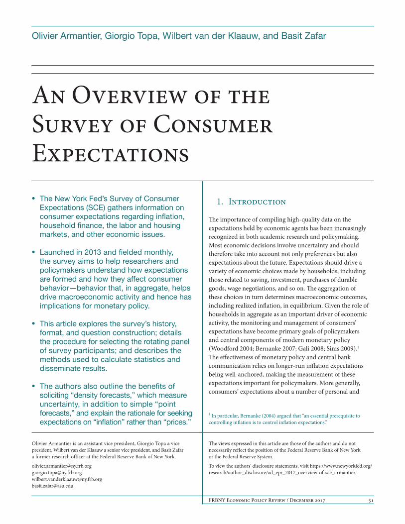
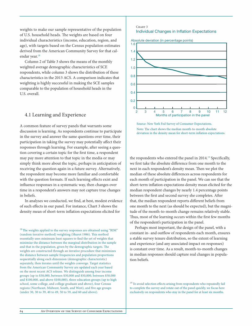
In analyses we conducted, we find, at best, modest evidence of such effects in our panel. For instance, Chart 3 shows the density mean of short-term inflation expectations elicited for

18 The weights applied to the survey responses are obtained using “RIM” (random iterative method) weighting (Sharot 1986). This method essentially uses minimum least squares to find the set of weights that minimize the distance between the marginal distribution in the sample and that in the population, given by the demographic targets. The weights are constructed through an iterative procedure that minimizes the distance between sample frequencies and population proportions sequentially along each dimension (demographic characteristic) separately, then iterates until the weights converge. Target statistics from the American Community Survey are updated each year based on the most recent ACS release. We distinguish among four income groups (up to $30,000, between $30,000 and $50,000, between $50,000 and $100,000, and above $100,000), three education groups (up to high school, some college, and college graduate and above), four Census regions (Northeast, Midwest, South, and West), and five age groups (under 30, 30 to 39, 40 to 49, 50 to 59, and 60 and above).

the respondents who entered the panel in 2014.19 Specifically, we first take the absolute difference from one month to the next in each respondent’s density mean. Then we plot the median of these absolute differences across respondents for each month of participation in the panel. We can see that the short-term inflation expectations density mean elicited for the median respondent changes by nearly 1.4 percentage points between the first and second survey she completes. After that, the median respondent reports different beliefs from one month to the next (as should be expected), but the magni-tude of the month-to-month change remains relatively stable. Thus, most of the learning occurs within the first few months of the respondent’s participation in the panel.

Perhaps most important, the design of the panel, with a constant in- and outflow of respondents each month, ensures a stable survey tenure distribution, so the extent of learning and experience (and any associated impact on responses) is constant over time. As a result, month-to-month changes in median responses should capture real changes in popula-tion beliefs.

19 To avoid selection effects arising from respondents who repeatedly fail to complete the survey and rotate out of the panel quickly, we focus here exclusively on respondents who stay in the panel for at least six months.

Absolute deviation (in percentage points)

Months of participation in the panel

0

0.2

0.4

0.6

0.8

1.0

1.2

1.4

1.6

12111098765432

Chart 3Individual Changes in Inflation Expectations

Source: New York Fed Survey of Consumer Expectations.Note: The chart shows the median month-to-month absolute deviation in the density mean for short-term inflation expectations.

FRBNY Economic Policy Review / December 2017 65

5. Computation and Reporting of SCE Statistics

To summarize and present our survey findings, we report median responses overall and by demographic characteris-tics. The median is a robust measure of central tendency that is less sensitive to the presence of outliers than the mean.20 Using a robust summary measure is important, since we do not delete or recode outliers in the SCE. In addition to the median, for some survey questions we also report the 25th and 75th percentiles of the distribution of responses, with the difference between the two quartiles, the IQR, representing a measure of dispersion or disagreement among respondents.

5.1 Quantile Interpolation

A common feature of response behavior when a survey question asks for a numerical response is the use of round-ing. When asked about past or expected future changes in percentage terms, almost all respondents appear to round to the nearest integer value. Accordingly, when changes in survey responses are tracked over time, it is common to see either no change in the computed raw median or a sudden abrupt change of one or more percentage points. In the case of grouped or rounded responses, it is therefore more infor-mative to compute instead the median (and other quantiles of the distribution of responses) using an interpolation method. Interpolated medians will better capture shifts in the frequencies of responses around the median.21 The same issue applies to other quantiles of the underlying distribution, including the first and third quartiles.

To compute interpolated quantiles, we use the symmetric linear interpolation approach proposed by Cox (2009).22 We provide details about the procedure in Appendix B. We have compared Cox’s procedure with other interpolation methods,

20 See Huber (1981) on robust statistics and estimation. Robust methods provide automatic ways of detecting, down-weighting (or removing), and flagging outliers, largely removing the need for manual screening and deletion of outliers.21 For example, consider two points x and y (with x < y) and two different empirical cumulative frequency distributions. The first empirical distribution attains the values 0.4 and 0.51 in x and y, while the second empirical distribution attains the values 0.49 and 0.6 in x and y. When the raw median is defined as the first value at which the cumulative distribution reaches or exceeds 0.5, the two empirical distributions both have the median of y. However, one may expect the median of the underlying continuous distribution to be closer to y for the first distribution and closer to x for the second distribution.22 In Stata, the procedure is implemented using the iquantile module. See Cox (2009).

including simple linear interpolation of the cumulative distribution function (asymmetric) and the Harrell-David procedure.23 Computed quantiles and month-to-month changes in quantiles are generally very similar.

5.2 Density Estimation

In addition to point forecasts and probabilities of binary events, we ask respondents in the SCE for their density forecasts of various continuous variables. As discussed in Section 2.3, we elicit these by asking individuals to assign probabilities to ranges or intervals of possible future realizations. In addition to future inflation (at the one- and three-year horizons), we elicit density forecasts for year-ahead national home price growth and, for those who are employed, year-ahead earnings growth (holding the job and the number of hours fixed).

In reporting and analyzing such density forecasts, we focus on two summary measures: the density mean and the density IQR, defined as the difference between the third and first quartile. To compute the density mean and density quartiles of each individual’s reported density, we use the reported bin probabilities to fit an underlying parametric density following the approach adopted by Engelberg, Manski, and Williams (2009). This approach is explained in detail in Appendix C.

Once fitted, the estimated density parameters are used to compute each individual respondent’s “density mean” and “density quartiles.” The mean represents the expected value, so in the case of the inflation density forecast, we refer to the computed density mean as the respondent’s “expected inflation rate.” Similarly, we use the estimated parameters to compute density quartiles, with the difference between a respondent’s 75th and 25th percentiles (the IQR) measuring the respondent’s “uncertainty.” When we aggregate across respondents, we obtain the median density mean (and the median density quartiles), which we use predominantly in our reports (as discussed in the next section).

An important and unique strength of the SCE is its ability to provide quantitative measures of overall uncertainty among respondents and changes therein over time. In our SCE releases, we report the (non-interpolated) median of the respondents’ IQRs as a summary measure of overall uncertainty in expectations. This statistic should not be confused with our measures of disagreement of expectations

23 In Stata, the procedure is implemented using the hdquantile module (Xiao 2006).

66 An Overview of the Survey of Consumer Expectations

among respondents. The latter are measured by the IQR of respondents’ point forecasts or the IQR of respondents’ density means, with both assessing dispersion in beliefs across respondents, while our uncertainty measure captures average forecast uncertainty among respondents.

5.3 Reporting of Multiple Medians

For several expectation questions, we solicit both point forecasts and density forecasts. For example, respondents are asked how much they expect the average home price to change nationwide over the next twelve months. They are also asked for the percent chance that, over the next twelve months, the average home price nationwide will increase (decrease) by: 12 percent or more; between 8 percent and 12 percent; between 4 percent and 8 percent; between 2 percent and 4 percent; and between 0 and 2 percent. As explained earlier, the latter bin probabilities are then used to fit the respondent’s underlying density of beliefs about year-ahead changes in home prices.

One would expect the respondent’s point forecast to rep-resent some summary statistic of the central tendency of his or her density, such as the density mean or median. While this often appears to be the case, with point forecasts largely tracking density means (as well as density medians), for a nontrivial subset of respondents the reported point forecasts correspond to values in the tails of the respondent’s density forecast. Similar findings were reported by Engelberg, Manski, and Williams (2009) for professional forecasters. An important advantage of using the density mean is that it captures the same measure across respondents. This might not be the case for point forecasts, which, for some respondents, may represent the density mean, while, for others, may represent the density median or mode or some other moment of the respondent’s forecast distribution. For this reason, in our monthly reporting of SCE findings, we place more emphasis on the median density mean, although we include both medians (of point forecasts and density means) in our interactive charts.

6. Dissemination of the Data

The monthly SCE findings are released on the second Monday of each month. The release takes the form of a press release24 as well as a set of interactive charts25 that show the trends in the different variables, both for the overall sample as well as various subgroups (such as by age or Census region). The underlying chart data are made available at the same time.

To facilitate the use of these data by researchers and policymakers, the micro data for the monthly survey are also released on the SCE web page with a nine-month lag. Open-ended responses and sensitive information (such as the respondent’s zip code) are not released.

The SCE project is still in its infancy, and the process of setting up web pages for the other data collected under the SCE umbrella (either as part of the ad hoc modules or the quarterly surveys) is ongoing. The SCE Credit Access Survey, which is conducted every four months and provides informa-tion on consumers’ experiences and expectations regarding credit demand and credit access, is available at https://www .newyorkfed.org/microeconomics/sce/credit-access#main; as in the case of the monthly survey, the micro data are made public with a nine-month lag. The annual SCE Housing Survey, which provides rich and high-quality information on consumers’ experiences, behaviors, and expectations related to housing, can be accessed at https://www.newyorkfed.org/microeconomics/sce/housing .html#main; the corresponding micro data are released with an eighteen-month lag. Interested readers should check the data page of the New York Fed's Center for Microeconomic Data for the latest products related to the SCE.26

24 Press releases are available at https://www.newyorkfed.org/press/ index.html#press-releases.25 Charts can be viewed at https://www.newyorkfed.org/microeconomics/sce.26 The Center for Microeconomic Data’s data page is https://www.newyorkfed.org/microeconomics/databank.html.

FRBNY Economic Policy Review / December 2017 67

Appendix A

Comparison of Consumer Confidence Survey (CCS) and American Community Survey (ACS) Samples

Full CCS Samplea 2013 ACS 2014 ACS

Percent

AgeUnder 30 3.7 10.8 10.630–39 11.3 16.9 16.940–49 15.7 19.2 18.750–59 23.9 20.8 20.660 and over 45.5 32.4 33.2

GenderFemale 47.7 49.9 49.9Male 52.3 50.1 50.1

EducationUp to high school NA 36.7 36.3Some college NA 31.3 31.2College graduate NA 32.0 32.5

IncomeUnder $15,000 8.3 13.0 12.6$15,000–$24,999 9.9 10.9 10.6$25,000–$34,999 10.3 10.3 10.1$35,000–$49,999 15.2 13.7 13.4$50,000–$74,999 19.7 17.9 17.8$75,000–$99,999 13.1 11.8 12.0$100,000–$124,999 9.4 7.9 8.1$125,000 or more 14.0 14.6 15.5

U.S. Census DivisionNew England 5.0 4.8 4.8Middle Atlantic 13.6 13.2 13.2East North Central 17.6 15.5 15.4West North Central 7.7 7.0 7.0South Atlantic 19.9 19.7 19.7East South Central 5.8 6.1 6.1West South Central 9.2 11.5 11.6Mountain 6.9 7.1 7.2Pacific 14.5 15.1 15.1

U.S. Census RegionNortheast 18.5 18.0 18.0Midwest 25.2 22.5 22.4South 34.9 37.3 37.4West 21.4 22.2 22.2

Sources: U.S. Census Bureau, American Community Survey (ACS); Conference Board, Consumer Confidence Survey (CCS).

Note: Each number in the table is the proportion of the sample that falls into that category.a CCS averages are unweighted averages, based on 64,133 CCS respondents during the October 2013 to September 2015 period.

Appendix

68 An Overview of the Survey of Consumer Expectations

AppendixAppendix A (Continued)

Number of responses

Mean

50th percentile

75th percentile

Day of month

0

20

40

60

80

100

120

31302928272625242322212019181716151413121110987654321

25th percentile

Survey Responses by Day of Month

Source: New York Fed Survey of Consumer Expectations. Note: The chart shows the mean and 25th, 50th, and 75th percentiles of the daily frequency of responses over all months from December 2012 to September 2015, thus combining months with different dates for the invitations and reminders.

FRBNY Economic Policy Review / December 2017 69

Appendix B: Quartile Interpolation

The main idea behind the approach proposed by Cox (2009) to interpolate the cumulative distribution (or quantile) function is the following: rather than linearly interpolating Pr(X < x) or Pr(X ≤ x), the average of the two, the mid-distribution function, Pr(X < x) + 0.5 Pr(X = x), is interpolated. More specifically, a brief description of the approach is as follows. First, for all observed values of x, compute the cumulative proportions, symmetrically considered, as CDFS(x) = Pr(X ≤ x) - 0.5Pr(X = x). Then to compute the median, determine the values of x observed with positive frequency with cumulative frequency CDFS that surround 0.5, defined as L (the smaller of the two) and H, and compute CDFS(L) and CDFS(H). Then the linearly interpolated median m is calculated as follows:

m = L + (H - L) × [0.5 - CDFS(L)] / [CDFS(H) - CDFS(L)].

Similarly for other quantiles, for example the third quartile, we identify the values of x observed with positive frequency with mid-distribution function values closest around 0.75, and in the equation above, replace 0.5 with 0.75. When applying sample weights, the CDFS values are computed by calculating frequencies Pr(X ≤ x) as sums of the relative weights (normalized to have mean 1) corresponding to all observations below or at x.

70 An Overview of the Survey of Consumer Expectations

Appendix C: Density Estimation

We follow the approach proposed by Engelberg, Manski, and Williams (2009) to fit a parametric distribution for each respondent based on the probabilities the respondent reported for each possible density interval. We assume the underlying distribution to have a generalized beta distribution when the respondent assigns positive probability to three or more outcome intervals. We assume an isosceles triangular distribution when the respondent puts all probability mass in two intervals and a uniform distribution when the respondent puts all probability mass in one interval.

The generalized beta distribution is a flexible four- parameter unimodal distribution that allows different values for its mean, median, and mode and has the following functional form:

0 if x < lf(x) = (x - l)α-1(r - x)β-1/B(α, β)(r-l)α + β - 1 if l ≤ < x ≤ r 0 if x > rwhere B(α, β) = Γ(α)Γ(β)/Γ(α, β).

It uses two parameters (α and β) to describe the shape of the distribution and two more (l and r) to fix the support of the distribution. Fitting a unique beta distribution requires a respondent to have assigned positive probability mass to at least three (not necessarily adjacent) intervals.27

27 In fitting a generalized beta distribution to a respondent’s bin probabilities, we use a minimum distance procedure that minimizes the distance between the empirical and estimated parametric distribution. We fix l and r to be the minimum and maximum bound of the positive-probability intervals, unless the corresponding bin is open-ended, in which case l and/or r are estimated together with α and β. In the latter case, we restrict l to be greater than or equal to -38 and restrict r to be at most 38. The sample statistics that we report are generally not sensitive to the choice of the imposed lower and upper bound.

The triangular distribution, for cases where a respondent assigns positive probability to exactly two adjacent bins, has the shape of an isosceles triangle whose base includes the interval with the highest probability mass and part of the adjacent interval. Thus, the triangle is anchored at the outer bound of the interval with probability mass above 50 percent.28 Its density has the functional form:

4 ___ (r - l)2 (x - l), l ≤ x ≤ (l + r)

___ 2 f(x) = 4

___ (r - l)2 (r - x), (l + r) ___ 2 ≤ x ≤ r

{

0 elsewhere.

With the triangle being anchored at one of the outer bounds (l or r), there is only one parameter (either l or r) to fit, which fixes the center and height of the triangle.29 Note that an isosceles triangle is symmetric, so the mean, median, and mode are identical to each other.

Densities are not fitted for respondents who put positive probability in only two bins that are nonadjacent or for whom the probabilities do not sum to 100. Such respondents make up less than 2 percent of our sample.

28 This rule applies only to the case of two adjacent intervals of equal width where neither interval is open-ended. In the case of two adjacent intervals with unequal width, the support of the triangle is assumed to include the smaller-width bin in its entirety if its probability exceeds 40 percent and includes the larger-width bin entirely otherwise, with the triangle covering only part of the adjacent bin. In the former case, the triangle would be anchored at the outer bound of the narrower bin and, in the latter, at the outer bound of the wider bin. In all cases where one of the two bins represents an open-ended interval (the left or right tail of the distribution), the base always includes the inner closed-end bin, with the triangle anchored by the innermost bound of the two intervals.29 In the case of two adjacent bins with equal width, no estimation is required, since the support of the triangle now fully includes both intervals, with the triangle anchored at the left-most and right-most interval bounds.

FRBNY Economic Policy Review / December 2017 71

ReferencesReferences

Armantier, O., W. Bruine de Bruin, S. Potter, G. Topa, W. van der Klaauw, and B. Zafar. 2013. “Measuring Inflation Expectations.” Annual Review of Economics 5: 273-301.

Armantier, O., W. Bruine de Bruin, G. Topa, W. van der Klaauw, and B. Zafar. 2015. “Inflation Expectations and Behavior: Do Survey Respondents Act on Their Beliefs?” International Economic Review 56, no. 2 (May): 505-36.

Armantier, O., W. van der Klaauw, S. Nelson, G. Topa, and B. Zafar. 2016. “The Price Is Right: Updating of Inflation Expectations in a Randomized Price Information Experiment.” Review of Economics and Statistics 98, no. 3 (July): 503-23.

Bernanke, B. 2004. “The Economic Outlook and Monetary Policy.” Speech at the Bond Market Association Annual Meeting, New York, N.Y.

———. 2007. “Inflation Expectations and Inflation Forecasting.” Speech at the Monetary Economics Workshop of the National Bureau of Economic Research Summer Institute, Cambridge, Mass.

Bruine de Bruin, W., C. F. Manski, G. Topa, and W. van der Klaauw. 2011. “Measuring Consumer Uncertainty about Future Inflation.” Journal of Applied Econometrics 26, no. 3 (April-May): 454-78.

Bruine de Bruin, W., S. Potter, R. Rich, G. Topa, and W. van der Klaauw. 2010a. “Improving Survey Measures of Household Inflation Expectations.” Current Issues in Economics and Finance 16, no. 7.

Bruine de Bruin, W., W. van der Klaauw, J. S. Downs, B. Fischhoff, G. Topa, and O. Armantier. 2010b. “Expectations of Inflation: The Role of Demographic Variables, Expectation Formation, and Financial Literacy.” Journal of Consumer Affairs 44, no. 2 (Summer): 381-402.

Bruine de Bruin, W., W. van der Klaauw, and G. Topa. 2011. “Expectations of Inflation: The Biasing Effect of Thoughts about Specific Prices.” Journal of Economic Psychology 32, no. 5 (October): 834-45.

Bruine de Bruin, W., W. van der Klaauw, G. Topa, J. S. Downs, B. Fischhoff, and O. Armantier. 2012. “The Effect of Question Wording on Consumers’ Reported Inflation Expectations.” Journal of Economic Psychology 33, no. 4: 749-57.

Cox, N. 2009. “IQUANTILE: Stata Module to Calculate Interpolated Quantiles,” http://EconPapers.repec.org/RePEc:boc:bocode:s456992.

Curtin, R. 2006. “Inflation Expectations: Theoretical Models and Empirical Tests.” Paper presented at the National Bank of Poland Workshop on The Role of Inflation Expectations in Modeling and Monetary Policy Making, Warsaw, February 9-10.

Delavande, A. 2014. “Probabilistic Expectations in Developing Countries.” Annual Review of Economics 6 (August): 1-20.

Delavande, A., X. Giné, and D. McKenzie. 2011. “Measuring Subjective Expectations in Developing Countries: A Critical Review and New Evidence.” Journal of Development Economics 94, no. 2 (March): 151-63.

Engelberg J., C. Manski, and J. Williams. 2009. “Comparing the Point Predictions and Subjective Probability Distributions of Professional Forecasters.” Journal of Business and Economic Statistics 27, no.1: 30–41.

Gali, J. (2008). Monetary Policy, Inflation, and the Business Cycle: An Introduction to the New Keynesian Framework. Princeton: Princeton University Press.

Huber, P. J. 1981. Robust Statistics. New York: Wiley.

Juster, T. 1966. “Consumer Buying Intentions and Purchase Probability: An Experiment in Survey Design.” Journal of the American Statistical Association 61: 658–96.

Leiser, D., and S. Drori. 2005. “Naïve Understanding of Inflation.” Journal of Socio-Economics 34: 179-98.

Manski, C. 2004. “Measuring Expectations.” Econometrica 72, no. 5 (September): 1329-76.

Sharot, T. 1986. “Weighting Survey Results.” Journal of the Market Research Society 28: 269-84.

72 An Overview of the Survey of Consumer Expectations

References

Sims C. 2009. “Inflation Expectations, Uncertainty, and Monetary Policy.” BIS Working Paper no. 275.

Svenson, O., and G. Nilsson. 1986. “Mental Economics: Subjective Representations of Factors Related to Expected Inflation.” Journal of Economic Psychology 7: 327-49.

Van der Klaauw, W., W. Bruine de Bruin, G. Topa, S. Potter, and M. Bryan. 2008. “Rethinking the Measurement of Household Inflation Expectations: Preliminary Findings.” Federal Reserve Bank of New York Staff Reports, no. 359, December.

Woodford, M. 2004: “Inflation Targeting and Optimal Monetary Policy.” Federal Reserve Bank of St. Louis Economic Review 86, no. 4 (July/August): 15-41.

Xiao, B. 2006. “The Use of the Interpolated Median in Institutional Research.” Paper presented at the Association for Institutional Research Annual Forum, Chicago, Ill.

The views expressed are those of the authors and do not necessarily reflect the position of the Federal Reserve Bank of New York or the Federal Reserve System. The Federal Reserve Bank of New York provides no warranty, express or implied, as to the accuracy, timeliness, completeness, merchantability, or fitness for any particular purpose of any information contained in documents produced and provided by the Federal Reserve Bank of New York in any form or manner whatsoever.