Embed Size (px)
Citation preview

1
An RL-based Scheduling Algorithm for Video Traffic in High-rate
Wireless Personal Area Networks
Shahab Moradi, A. Hamed Mohsenian-Rad, and Vincent W.S. Wong
Department of Electrical and Computer Engineering
The University of British Columbia, Vancouver, Canada
e-mail: shahab, hamed, [email protected]
Abstract: The emerging high-rate wireless personal area network (WPAN) technology is capable
of supporting high-speed and high-quality real-time multimedia applications. In particular, video
streams are deemed to be a dominant traffic type, and require quality of service (QoS) support.
However, in the current IEEE 802.15.3 standard for MAC (media access control) of high-rate
WPANs, the implementation details of some key issues such as scheduling and QoS provisioning
have not been addressed. In this paper, we first propose a Markov decision process (MDP) model
for optimal scheduling for video flows in high-rate WPANs. Using this model, we also propose
a scheduler that incorporates compact state space representation, function approximation, and
reinforcement learning (RL). Simulation results show that our proposed RL scheduler achieves
nearly optimal performance and performs better than F-SRPT, EDD+SRPT, and PAP scheduling
algorithms in terms of a lower decoding failure rate.
Keywords: Wireless personal area networks, scheduling, QoS, ultra-wide band (UWB), Markov
decision process (MDP), reinforcement learning.
This paper was presented in part in IEEE Global Telecommunications Conference (Globecom),
Washington, DC, December 2007.

2
I. INTRODUCTION
In recent years, ultra-wide band (UWB) technology has received increasing attention in the
wireless world. It provides short-range connectivity, low transmit power levels, and high-data
rates. This makes UWB be the physical layer of choice for high-rate wireless personal area
networks (WPANs). UWB-enabled WPANs can offer many new applications, such as home
entertainment, real-time multimedia streaming, and wireless universal serial bus (USB).
In order to fully exploit UWB technology in high-rate WPANs, upper layers, including the
media access control (MAC) layer, must be properly designed for high-rate applications. Video
transmission is one such application for high-rate WPANs, which is predicted to constitute a
major traffic load. Real-time video flows are delay-sensitive and require quality of service (QoS)
guarantee. However, in the IEEE 802.15.3 standard for MAC [1], which is designed for WPANs,
details of scheduling and QoS support are left to the developers. Consequently, in this paper, we
aim to design an application-aware scheduling algorithm for MAC layer to provide the required
QoS for video traffic.
Similar to other real-time traffic, video flow is delay sensitive and its frames are dropped at
the receiver if their delay exceeds the maximum tolerable delay. However, video stream has a
few unique characteristics that make QoS support more challenging than other real-time traffic.
It has large peak-to-average ratio of the frame sizes and hierarchical structure with dependency
among its frames [2].
Recently, various MAC scheduling algorithms have been proposed for high-rate WPANs (e.g.,
[2]–[10]). For impulse-based UWB, scheduling problems can be formulated as rate and power
allocation problems. These problems can be modeled as a joint optimization problem, so as to
minimize the total power consumption [7] or maximize the total system throughput [9]. The
concept of exclusion region is also used for such schedulers [10]. On the other hand, with no
assumption on the type of physical layer, Mangharam et al. proposed the fair shortest remaining
3
processing time (F-SRPT) scheduler [5]. SRPT schedules different jobs in the system in the
order of their remaining processing time, from the shortest to the longest. F-SRPT is a variation
of SRPT that maintains fairness among flows with different data rates. In [6], the earliest due
date (EDD) method is used along with SRPT. In [11], Rhee et al. used the application layer
information at MAC layer. Each device informs the piconet controller of the maximum size
of its I , P , and B frames for video flows. The channel time is then allocated based on these
values. Kim and Cho proposed a scheduling algorithm designed for MPEG-4 flows [2]. Each
MPEG-4 frame type is scheduled with a pre-assigned priority (PAP) in I , P , and B order.
The scheme proposed in [8] focuses on reducing the average waiting time by using an M/M/c
queuing model for channel time allocation at the piconet coordinator. It also proposed a command
aggregation scheme in order to reduce MAC overhead when sending short command frames.
Energy efficiency is considered by the scheduler proposed in [12]. It defines different service
categories in order to balance between energy efficiency and QoS. It also uses the application
layer information to assign priorities to the buffered frames at the source of a flow. In [13], we
proposed a frame-decodability aware (FDA) technique to improve the performance of scheduling
of video flows.
The objective of our work is to design a systematic scheduling algorithm for video flows in
high-rate WPANs. The contributions of in this paper are as follows:
• We provide a mathematical framework based on Markov decision process (MDP) to deter-
mine the optimal scheduler for video flows in high-rate WPANs. This framework takes into
account the number and pattern of video flows, and their hierarchical structure.
• Using the MDP framework, along with compact state space representation, function ap-
proximation, and reinforcement learning (RL), we propose a practical scheduling algorithm
which can provide significantly better QoS to video flows when compared to some other
schedulers [14].
• Simulation results show that our proposed RL scheduler achieves nearly optimal perfor-
4
mance and performs 53%, 42%, and 49% better than F-SRPT, EDD+SRPT, and PAP
schedulers, respectively [15].
The rest of this paper is organized as follows. In Section II, we provide an overview of the
IEEE 802.15.3 standard for MAC, the hierarchical structure of video streams, related scheduling
algorithms, the performance metrics for video flows, and reinforcement learning. In Section III,
we describe the mathematical formulation for the optimal video scheduler. The implementation
mechanisms of the RL algorithm are described in Section IV. Section V describes an extension
of our proposed model. Results for performance evaluations and comparisons are presented in
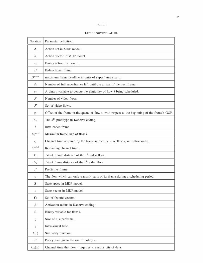
Section VI. Conclusions and future work are discussed in Section VII. A list of nomenclature
is in Table I.
II. BACKGROUND
A. IEEE 802.15.3 MAC Standard
The IEEE 802.15.3 is designed for WPANs and aims to provide low cost, low power consump-
tion, and high data rate communications, within its area of operation called the piconet [1]. A
piconet consists of a number of independent devices (DEVs) that communicate with each other
under the control of the piconet coordinator (PNC). The PNC provides basic timing, performs
scheduling, and manages the QoS requirements of the piconet.
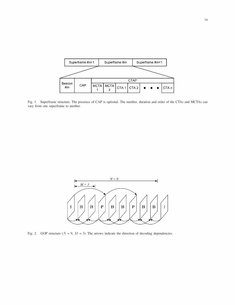
Within a piconet, the timing is based on superframes, which consists of three parts (see Fig. 1).
The first part, beacon, announces timing allocations, superframe duration, and other piconet
synchronization parameters. The second part, the contention access period (CAP), is used to
communicate commands and asynchronous data. The third part, channel time allocation period
(CTAP), is composed of channel time allocations (CTAs) and management CTAs (MCTAs). A
DEV can use its CTA, which is assigned to it by the PNC, for isochronous streams, asynchronous
data transfer, or sending commands. Channel access during CTAP is TDMA and there is no
5
contention in this period. By sending beacon at the beginning of superframe, the PNC announces
the start time and duration of each CTA as well as the DEVs that are allowed to use it.
As the central coordinator, PNC is responsible for scheduling. Depending on the scheduling
algorithm, PNC requires certain information such as the number of flows, their reserved rates,
their queues’ status, and type and deadline of the frames in their queues, in order to allocate
CTAs to different flows.
B. Video Streams
A typical video encoder generates a sequence of three types of compact frames: intra-coded
(I), predictive (P ), and bidirectional (B) frames [16]. Because of the different compression
schemes used to encode the different frame types, I frames tend to be larger (less compressed)
than P and B frames, and P frames tend to be larger than B frames. Video encoders generate
the three frame types according to a predefined pattern called group of pictures (GOP). This
pattern is characterized by two parameters (N, M), where N is the I-to-I frame distance, and
M is the I-to-P frame distance [16]. This pattern is generally fixed for a given video sequence,
and N is a multiple of M . Fig. 2 illustrates the hierarchical structure of video streams, as well as
decoding dependencies among the frames. In order for a frame to be decodable at the receiver,
all other frames that it depends on, including the frame itself, must be available at the receiver. A
frame is undecodable if it is directly or indirectly lost [17]. Direct loss happens when the receiver
does not receive the frame completely, either because of channel error or deadline expiration. A
frame is indirectly lost when some frames that it depends on are directly lost. As an example,
in Fig. 2, all the frames in a GOP depend on the only I frame in that GOP; therefore, if that
I frame does not meet its deadline, the whole GOP is considered undecodable (direct loss of
the I frame and hence, indirect loss of the rest of the frames). For instance, with N = 12 and
frame rate of 30 frames per second (fps), this would result in impaired quality for about 360
ms, which is fairly obvious to a user. Similarly, loss of P frames can also degrade the quality of

6
video streams. Table II shows the number of frames depending on each frame inside a GOP. The
larger the number of dependencies on a frame, the more important that frame is for decoding
process at the receiver. Consequently, video frame types can be ranked, from the most important
to the least important, as I , P , and B.
C. Scheduling Algorithms
In an 802.15.3 piconet, the CTA requirements of a flow can be regarded as a job. It has been
shown that the Shortest Remaining Processing Time (SRPT) scheduling algorithm minimizes the
number of pending jobs in the system, and thus minimizes the average waiting time of the jobs
[18]. It schedules different jobs in the system in the order of their remaining processing time,
from the shortest to the longest. In the preemptive case, SRPT switches to a newly arrived job
if the processing time of that job is shorter than the job currently being served.
In systems with heterogeneous flows that have different average data rates, SRPT favors the
flows with smaller average data rate since they tend to have smaller frames. In [5], Mangharam
et al. proposed a variation of SRPT, which maintains fairness among flows with different data
rates. This scheduling algorithm, called Fair-SRPT (F-SRPT), first normalizes the size of the
frames belonging to a flow to the mean rate of that flow. This normalized size is then used by
SRPT to sort the frames. As a result of the normalization in the first step, flows with smaller
mean data rate will not dominate channel access. Hence, network resources are allocated in a
fair manner. The channel time allocation algorithm proposed in [5] guarantees that all the flows
receive at least as much as their reserved amount of CTA. If a flow does not require all of its
reserved CTAs (i.e., under-loaded), the excess is added to the idle channel time. This idle channel
time is shared among the overloaded flows, which require more CTA than their reservation.
The optimality of SRPT, in that it minimizes the average waiting time of the jobs in the
system, holds only when the jobs have no delay constraint. Thus, in the systems with delay
sensitive traffic, SRPT need not be the best scheduler, and using deadline information can yield

7
better performance. One scheduler that considers the deadline of the frames is the earliest due
date (EDD). It schedules the frames in the order of their deadlines, from the earliest on. It
is proven that EDD policy minimizes the probability of packet dropping in the system due to
delay violation [19]. However, in WPANs, where the PNC should be informed of the internal
state of the system queues, it is not practical to convey the exact deadline. This information
is represented in a quantized form, usually with respect to the superframe size. A DEV may
inform the PNC that the frame in its queue will expire after j full superframes. As a result of
quantization, many frames may have equal deadlines, hence a tie-breaking method is needed.
In [6], Torok et al. used EDD along with SRPT as the tie-breaking method. They studied the
performance of this scheduler under real-time traffic with variable frame sizes. They modeled
this traffic with batch arrival process. Each batch is the MAC fragments of a frame and all have
the same deadline. In addition, the inter-arrival time of the batches is equal to the inter-arrival
time of the frames and can be constant or variable. For each flow, PNC has the information
about the size and deadline of its first (head-of-the-queue) frame, as well as the total size of
its queue. EDD+SRPT scheduler first selects the flows based on the deadline of the first frame
in their queue (i.e., according to EDD). If the first frame of several flows have equal deadline,
then they are scheduled in ascending order of their frame size (i.e., according to SRPT). After
serving the frames closest to expiration, the remaining channel time, if any, is allocated to the
flows according to their total queue size using SRPT algorithm.
The pre-assigned priority (PAP) in [2] schedules video frames their importance (i.e., in I , P ,
and B order). EDD and SRPT are used to break ties among frames of the same type, when
they cannot be served together in one superframe. The work in [2] used mini packets with short
duration for signaling purposes. This method divides the CTAP part of the superframe into two
parts. The first part is CTA and is used for transmission of real-time traffic. The second part is
Feedback CTAs (FCTAs). The PNC allocates this part for transmission of mini packets. There
are two classes of information contained in the mini packets. The first class is used for CTA

8
allocation to video flows in the system. This includes data rate, ACK policy and fragmentation
threshold between source and destination of the flow, as well as video frame type and queue
status information of the source of the flow. These pieces of information are contained in the mini
packet only when necessary (i.e., when their value changes). The second class of information is
used for deciding the allocation of FCTA for mini packets. In order not to waste channel time
with unused FCTA, it is only allocated to the DEVs that need to send mini packet to the PNC
(i.e., when a new video frame arrives at the DEV). Therefore, this class of information includes
the time of the next arrival. By using that information, the PNC can allocate FCTAs only to
the flows that need it. After receiving all the mini packets from the DEVs, the PNC performs
scheduling based on the received information.
D. Performance Metrics: JFR and DFR
Video frames, like other real-time traffic, are delay sensitive. The video frames will be dropped
at the receiver if their delay exceeds the maximum tolerable delay. This is the base of job failure
rate (JFR) criterion for evaluating performance of schedulers in the MAC layer. For a delay
sensitive flow, JFR is defined as the fraction of frames that do not meet their transmission
deadlines, and are hence useless and get dropped. An important consequence of hierarchical
structure of video stream is that JFR, by itself, cannot accurately reflect the QoS given to a
video flow at the MAC layer. In other words, low JFR does not necessarily indicate high QoS.
As a result, another performance metric is required for comparing the performance of different
schedulers. We use the decoding failure rate (DFR) criterion, which takes frame dependencies
into account. DFR is defined as the ratio of the total number of undecodable frames to the
total number of frames [17]. DFR can be viewed as an objective measure of user-perceived
degradation of quality, and is the main performance metric in this paper.
9
E. Reinforcement Learning (RL)
In many real-life sequential decision making problems, dynamic programming (DP) techniques
are not practical because of two main reasons. First, the agent may not have complete knowledge
about dynamics of the system or environment. Second, when the system state and/or action space
is huge (e.g., continuous state spaces), it is not feasible to exploit DP. The former problem is
called curse of modeling, while the latter is called curse of dimensionality. Reinforcement learning
(RL) combines DP methods with other methods including stochastic approximation and function
approximation to tackle these problems [20]. In RL, an agent should learn a policy (i.e., how to
map situations to actions) through trial and error. The agent is not provided with the policy, but
instead it must discover which actions yield the most reward by trying them. In an RL model,
the agent has an indication of the system state. The agent takes action, which leads the system
to another state. The value of this state transition is communicated to the agent through a scalar
reinforcement signal (or reward). The agent should choose actions that tend to increase some
function of the reward. Similar to DP, this function can be average discounted reward, average
reward, or other reward functions. Unlike DP, however, the agent should learn to maximize this
function over time by systematic trial and error, guided by a wide variety of algorithms [20]
[21]. The system environment can be either real or simulated. If a simulator is used, complete
knowledge of the random variables that govern the system dynamics is required [22].
In order to obtain a lot of rewards, the agent should be greedy; i.e., it should choose the actions
that it has discovered to produce a lot of reward. In other words, it should exploit its current
experience. However, there might exist better actions that the agent has not yet discovered or
explored. As a result, if the agent occasionally deviate from the greedy manner (i.e., perform
exploration), chances are that it can find better actions. The dilemma in RL is that neither
exploration nor exploitation should be pursued exclusively. In fact, one of the challenges of RL
is to balance the trade-off between exploitation and exploration. The agent must try a variety of

10
actions and progressively favor those that appear to be best. On a stochastic task, each action
must be tried many times to gain a reliable estimate of its expected reward [21].
When the agent does not have the system model, it should build a knowledge base according
to its interaction with the system. In Q-learning, this knowledge base is made up of factors
called Q-values. For each state s ∈ S and each action a ∈ As, the agent saves a Q-value Q(s, a)
and updates these values as the agent learns. Before the learning begins, all the Q-values are
set to the same value. At a decision epoch, when the system is in state s, the agent chooses an
action a that maximizes the Q-value (i.e., a = arg maxa′∈AsQ(s, a′)). The simulator will then
simulate the chosen action a in the current state s and evolve to the new state s′. It also gives the
accrued reward and the time spent during the state transition. The learning algorithm embedded
in the agent will then use this information to update Q(s, a). Basically, Q(s, a) increases if a
was a good action (i.e., good actions are rewarded), and decreases otherwise. An exclusively
greedy learning algorithm is not the best. Consequently, the agent should occasionally explore
and choose an action other than the one with the maximum Q-value. Over time, as the agent
explores and tries out all the state-action pairs often enough, it learns the best action in each
state. In other words, it learns an optimal (or near-optimal) policy. At this point, the agent should
cease exploration and follow the learned optimal policy in a greedy manner.
Most of the RL algorithms in the literature, including Q-learning, are based on the dis-
counted reward optimality criterion. Moreover, these algorithms cannot automatically extend
to the average reward criterion [23]. As we will show in Section III-D, the average reward
criterion is more suitable for our scheduling problem. We use an algorithm called SMART
(Semi-Markov Average Reward Technique) [24] [25] [26] that is designed for average reward
RL. The convergence analysis of this algorithm is given in [25] and it has been successfully
applied to different problems including production inventory [24], airline seat allocation [26],
and QoS provisioning in wireless cellular networks [23]. The difference between Semi-Markov
decision process (SMDP) and Markov decision process (MDP) is that for SMDP, the time that

11
it takes the system to transit from one state to the other is stochastic. MDP is a special case
of SMDP when the state transition duration is fixed. Since in Section III we formulate the
scheduling problem in the form of an MDP, we can use this algorithm with fixed state transition
duration.
III. OPTIMAL SCHEDULING ALGORITHM FOR VIDEO TRAFFIC
In this section, we formulate the problem of finding the scheduling policy with minimum
average DFR in the form of a Markov decision process (MDP) with average reward criterion
[27]. We then relate the gain of the scheduling policy with the average DFR that it yields. As
a result of the linear relationship between gain and average DFR, we can use reinforcement
learning (RL) techniques [20] [21] to find the scheduling policy which minimizes average DFR.
Consider a WPAN and let F denote the total number of video flows. We denote F =
1, 2, . . . , F as the set of all flows. We assume that the deadline of all video frames is fixed1,
and is equal to the frame inter-arrival time γ. As a result, the queue of each flow holds no
more than one frame at any time. We denote the GOP pattern of the ith video flow (i ∈ F ) by
(Ni, Mi), where Ni and Mi are the I-to-I and I-to-P frame distance, respectively. The GOP
pattern of all flows is assumed to remain constant during the flows’ lifetime. An MDP problem
formulation includes the set of decision epochs, the set of system states, the set of actions, the
reward function, and the state transition probabilities. We define these elements for our MDP in
the following subsections.
A. Decision Epochs
The scheduler should make a decision at the beginning of each superframe, and decide to
schedule which flows in that superframe. The superframe size η is assumed to be fixed and
1Notice that a tight fixed deadline indicates the worst-case scenario in which the source codec has no buffering capability;
thus, it can only handle one frame every γ (i.e., frame inter-arrival time) seconds.

12
is less than γ. For simplicity, we show the decision epochs in terms of superframe size. For
example, the actual time of decision epoch n, which is the beginning of the nth superframe, is
(n− 1)η. Therefore, the set of decision epochs is 1, 2, . . . , T.
B. States
Let the function txi(x) denote the amount of channel time that flow i requires to send x bits of
data. The simplest form of this function is txi(x) = x/channel data ratei. However, depending
on the acknowledgement policy, inter-frame spacing times, and maximum MAC fragment size,
this function can have a different form. Moreover, assume that the maximum frame size of flow
i is Lmaxi . We define the set of possible system states as follows:
S ,
s = (l,d, g, δ) | ∀ i ∈ F : 0 ≤ li ≤ txi(Lmaxi ),
di ∈ 0, . . . , Dmax, gi ∈ 0, . . . , Ni − 1, δi ∈ 0, 1
, (1)
where
• l , [l1 l2 · · · lF ], and li is the channel time required by the frame in the queue of flow i,
in milliseconds.
• d , [d1 d2 · · · dF ], and di is the number of full superframes remaining until the arrival
of the next frame of flow i. Since the maximum tolerable delay for video frames is the
frame inter-arrival time, di can alternatively be interpreted as the deadline of the frame in
the queue of flow i, in terms of superframe size.
• g , [g1 g2 · · · gF ], and gi is the offset of the frame in the queue of flow i, with respect to
the beginning of the frame’s GOP of flow i. For the first frame of the GOP gi = 0, and for
the last one gi = Ni − 1.
• δ , [δ1 δ2 · · · δF ], and δi is a binary variable which denotes whether the current frame in
the queue of flow i can be decoded successfully at the receiver. δi is set to 0 if any I or
13
P frame, on which the current frame of flow i depends, is directly lost; and is equal to 1
otherwise.
• Dmax , ⌊γ
η⌋, is the maximum frame deadline in units of superframe size η, where ⌊·⌋ is
the floor function.
The scheduler incorporates the FDA technique [13], [14] to determine the value of δ based
on l, d and g.
C. Actions
Let A be the set of all possible actions. We have,
A =
a , (a1, a2, · · · aF , p) | p ∈ F ∩ 0; ai ∈ 0, 1, ∀ i ∈ F ; ap = 0 if p 6= 0
, (2)
where ai is equal to 1 if the scheduler allocates enough channel time to flow i so that it can fully
transmit its frame. Otherwise, it is equal to 0. The parameter p is the flow that can only transmit
parts of its frame during the channel time that the scheduler allocates to it. If no such flow exists,
then p = 0. Here we assume that in each superframe, the scheduler allows at most one partial
frame transmission, and the rest are full frame transmissions. To explain this, we notice that in
general, we are not interested in partial transmissions as a half (incomplete) frame is not useful
for a video decoder at the destination node. In fact, we will see that our introduced rewarding
function in Section III-D only rewards full transmissions. Nevertheless, we still allow a single
long (i.e., almost complete) partial transmission as it is more similar to a full transmission.
The last conditional statement in (2) implies that the frame of flow p cannot be both fully and
partially transmitted simultaneously.
At each decision epoch, the scheduler should choose an action depending on the current state.
The chosen action must satisfy a few constraints. First, the channel time required to transmit
scheduled frames should not be more than the superframe length η:
F∑
i=1
(ai · li) ≤ η. (3)
14
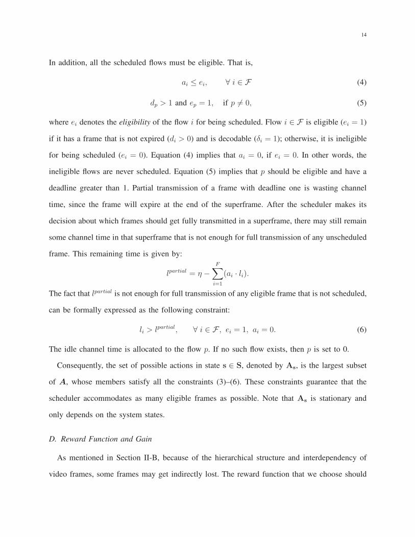
In addition, all the scheduled flows must be eligible. That is,
ai ≤ ei, ∀ i ∈ F (4)
dp > 1 and ep = 1, if p 6= 0, (5)
where ei denotes the eligibility of the flow i for being scheduled. Flow i ∈ F is eligible (ei = 1)
if it has a frame that is not expired (di > 0) and is decodable (δi = 1); otherwise, it is ineligible
for being scheduled (ei = 0). Equation (4) implies that ai = 0, if ei = 0. In other words, the
ineligible flows are never scheduled. Equation (5) implies that p should be eligible and have a
deadline greater than 1. Partial transmission of a frame with deadline one is wasting channel
time, since the frame will expire at the end of the superframe. After the scheduler makes its
decision about which frames should get fully transmitted in a superframe, there may still remain
some channel time in that superframe that is not enough for full transmission of any unscheduled
frame. This remaining time is given by:
lpartial = η −F∑
i=1
(ai · li).
The fact that lpartial is not enough for full transmission of any eligible frame that is not scheduled,
can be formally expressed as the following constraint:
li > lpartial, ∀ i ∈ F , ei = 1, ai = 0. (6)
The idle channel time is allocated to the flow p. If no such flow exists, then p is set to 0.
Consequently, the set of possible actions in state s ∈ S, denoted by As, is the largest subset
of A, whose members satisfy all the constraints (3)–(6). These constraints guarantee that the
scheduler accommodates as many eligible frames as possible. Note that As is stationary and
only depends on the system states.
D. Reward Function and Gain
As mentioned in Section II-B, because of the hierarchical structure and interdependency of
video frames, some frames may get indirectly lost. The reward function that we choose should

15
account for this fact. We give a reward of one unit when a frame is scheduled. On the other
hand, if the deadline of a frame expires, the scheduler receives a penalty (negative reward) of
W units, where W is the number of frames that depend on the expired frame. Table II shows
the number of dependencies between GOP frames of an (N, M) video flow.
Let ci(s) be the state-dependent penalty (or cost) function for flow i:
ci(s) =
(
Ni + (Mi − 1))
· ei · Udi=1, if yi(gi) = I,
ei · Udi=1, if yi(gi) = B,(
Ni − 1− ( gi
Mi− 1)Mi
)
· ei · Udi=1, if yi(gi) = P ,
where the function yi(g) : 0, . . . , Ni − 1 → I, B, P maps g to frame types as follows:
yi(g) =
I, if g = 0,
B, if g mod Mi ≥ 1,
P, if g mod Mi = 0 and g 6= 0.
Furthermore, U· is the indicator function and is equal to 1 if its argument is true, and is 0
otherwise. The product ei(n) × Udi(n)=1 indicates if the flow i has an urgent eligible frame.
Hence, the scheduler should receive ci(s(n)) units of penalty if it does not schedule the frame
of flow i in the current superframe.
As a result, we can express the state- and action-dependent reward that the scheduler receives
at superframe n by:
r(s(n), a(n)) =F∑
i=1
[
ai(n)− ci(s(n))(1− ai(n))
]
. (7)
In order to show the merits of the reward function in (7), we study the policy gain that it yields.
The gain of policy π under the average reward criterion is the average accumulated reward. In
our formulation, the policy gain is given by:
ρπ =1
T
T∑
n=1
r(s(n), a(n))
=F∑
i=1
(
∑Tn=1 ai(n)−
∑Tn=1 ci(s(n))(1− ai(n))
T
)
. (8)

16
The total number of frames for each flow is total frames = total timeinter arrival time
= ηT
γ. Furthermore, the
terms∑T
n=1 ai(n) and∑T
n=1 ci(s(n))(1− ai(n)) in (8) are in fact the total number of scheduled
frames and the total number of undecodable frames for each flow, respectively. In addition, these
two terms sum up to the total number of frames for flow i. Consequently, equation (8) can be
rewritten as:
ρπ =η
γ
F∑
i=1
( total scheduled− total undecodable
total frames
)
=η
γ
F∑
i=1
(
1−2× total undecodable
total frames
)
=η
γ
F∑
i=1
(1− 2DFRπi )
=ηF
γ−
2η
γ
F∑
i=1
DFRπi , (9)
where DFRπi is the decoding failure rate of flow i under the policy π. Let DFR
π, 1
F
∑Fi=1 DFRπ
i
denote the average DFR under the policy π. Using (9), we have
DFRπ
=1
2−
γ
2ηFρπ. (10)
Equation (10) shows that in our formulation, the average DFR is a linear function of gain.
Therefore, we conclude that:
arg maxπ
ρπ = arg minπ
DFRπ. (11)
Hence, an optimal (maximum) gain policy yields the optimal (minimum) average DFR, which
is what we aim to find.
E. State Transitions
Assume that at superframe n, the system is in state s(n) and chooses the action a(n). In this
section, we determine the system state at superframe n+1, s(n+1). This state depends on s(n),
a(n) and new frame arrivals. We determine the state transitions per flow, i.e., we show how the

17
state variables relate to each flow change. The whole system state is updated by performing the
same procedure for all the flows.
When di(n) ≥ 1, no new video frame will arrive for flow i. Thus, the remaining time until
the next arrival is reduced by one superframe. If the flow is scheduled, its length will become 0.
And if it is partially transmitted, its length will reduce by lpartial. Otherwise, the length remains
unchanged. The frame offset within GOP also does not change. The value of δi changes only
when an I or P frame of flow i expires, or when a new GOP starts, which is indicated by arrival
of a new I frame for flow i. None of these happens when di(n) ≥ 1. Hence, if di(n) ≥ 1, then
the state deterministically changes as follows:
di(n + 1) = di(n)− 1,
li(n + 1) = li(n)(1− ai(n))− lpartialUi=p,
gi(n + 1) = gi(n),
δi(n + 1) = δi(n).
When di(n) = 0, it means that the frame in the queue of flow i has expired, if it has not
already been sent, i.e., if li(n) 6= 0. It also means that a new frame will arrive for flow i, within
superframe n. We denote the deadline and channel time requirement of the newly arrived frame
for flow i within superframe n by dnewi (n) and lnew
i (n), respectively.
Let probi(lnewi (n)) denote the probability that the channel time request of flow i is lnew
i (n).

18
Thus, when di(n) = 0 ,the state changes with probability probi(lnewi (n)) as follows:
di(n + 1) = dnewi (n),
li(n + 1) = lnewi (n),
gi(n + 1) = (gi(n) + 1) mod Ni,
δi(n + 1) =
1, if yi(gi(n + 1)) = I,
0, if yi(gi(n)) = I, P and li(n) 6= 0,
δi(n), otherwise,
This probability is simply related to the frame size distribution probability of flow i.
IV. ALGORITHM IMPLEMENTATION: RL SCHEDULER
In this section, we discuss how to find the optimal gain policy defined by the MDP given
in the previous section. Our formulation has modeling and dimensionality issues, so dynamic
programming cannot be used. First, we do not have the knowledge of the state transition
probabilities, because the scheduler does not know the frame size distribution of the video flows
beforehand. We use the SMART algorithm [24] to overcome the curse of modeling. Second, in
the state space defined in equation (1) we have one continuous variable, i.e. the frame length.
Even if we quantize this variable to several levels, the state space would still be huge. For
instance, suppose that Dmax = 4 and Ni = 12 for all i ∈ F , and we quantize li’s to 8 levels.
Thus, |S| = (8 × 5 × 12 × 2)F≈ 1000F . Furthermore, it is easy to verify that |A| = F · 2F .
The semi-Markov average reward techique (SMART) learns the Q-function Q : S×A→ R,
which has impractical memory requirement and convergence rate given the size its domain. To
tackle this issue, we solve the problem in two phases. In Section IV-A, we describe a compact
representation of the state-action space, which is a mapping from S × A to a smaller set Ω.
Then, in Section IV-B, a memory-based function approximator is used to map Ω to the set of
real numbers R.
19
A. Features and State Space Representation
We use an aggregation scheme [21], which gives a more compact representation of the
state-action space. This scheme is useful when we have knowledge of an initial part of the
environment’s dynamics but not necessarily of the full dynamics. For instance, in our formulation,
the effect of chosen action on the system state can be deterministically simulated by the scheduler.
On the other hand, the new frame arrivals cannot be deterministically simulated. Using this
scheme, we obtain a more efficient learning method by breaking the environment’s dynamics
into the immediate effect of the action, which is deterministic and perfectly known, and the arrival
process of new frames with unknown size distribution [21]. We refer to the system state after
the effect of the taken action as afterstate [21]. The actual system state in the next superframe
is the afterstate updated according to the new frame arrivals.
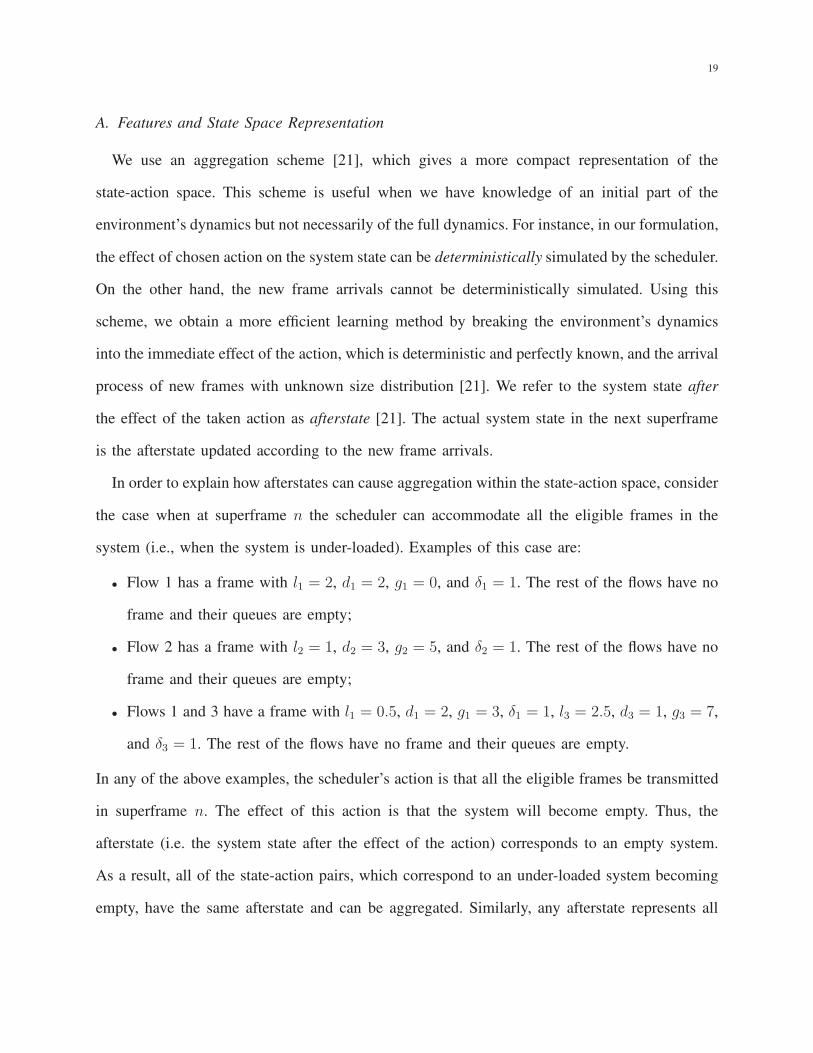
In order to explain how afterstates can cause aggregation within the state-action space, consider
the case when at superframe n the scheduler can accommodate all the eligible frames in the
system (i.e., when the system is under-loaded). Examples of this case are:
• Flow 1 has a frame with l1 = 2, d1 = 2, g1 = 0, and δ1 = 1. The rest of the flows have no
frame and their queues are empty;
• Flow 2 has a frame with l2 = 1, d2 = 3, g2 = 5, and δ2 = 1. The rest of the flows have no
frame and their queues are empty;
• Flows 1 and 3 have a frame with l1 = 0.5, d1 = 2, g1 = 3, δ1 = 1, l3 = 2.5, d3 = 1, g3 = 7,
and δ3 = 1. The rest of the flows have no frame and their queues are empty.
In any of the above examples, the scheduler’s action is that all the eligible frames be transmitted
in superframe n. The effect of this action is that the system will become empty. Thus, the
afterstate (i.e. the system state after the effect of the action) corresponds to an empty system.
As a result, all of the state-action pairs, which correspond to an under-loaded system becoming
empty, have the same afterstate and can be aggregated. Similarly, any afterstate represents all

20
the state-action pairs that result in that afterstate. Using afterstates is in fact a mapping from
S×A to S. Reference [28] successfully applies this idea to admission control problem in cellular
networks.
The state space of our MDP has binary variables in δ, continuous variables in l, and integer
variables in d and g. Even after using afterstates, the scheduler should learn the Q-function over
S, which is still very large. Therefore, we need to specify the important features in each afterstate,
which most affect the scheduling decision. As mentioned before, there is no systematic way of
choosing the features. We approach this task by studying the behavior of the SRPT, EDD and
PAP schedulers. All of these schedulers can be viewed as single-stage decision making process,
where the scheduler chooses an action merely based on its immediate effect, i.e., based on
the resulting afterstate. SRPT uses information about length. Since it minimizes the number of
pending frames in the system, it chooses an action that yield an afterstate with minimum number
of frames. In other words, the only feature of the afterstate that is important for SRPT is the
number of frames in the system. Similarly, EDD+SRPT uses the number of frames in the system,
but groups them according to their deadlines. It chooses an action that leads to the afterstate with
the minimum number of frames in the group with the smallest deadline. If this value is the same
for the afterstates of two actions or more, the size of the group with second smallest deadline
is used, and so on. Therefore, the features that EDD+SRPT used are the number of frames in
each deadline group. PAP, which is an application-aware scheduler, further partitions the frames
in the system according to their type. In other words, SRPT, EDD+SRPT, and PAP schedulers
mainly focus on the information about length, deadline, and type, respectively. With the addition
of FDA technique, they can take advantage of decodability as well. Since the optimal scheduler
should focus on all the information, it is reasonable to assume that it uses all the features used
by those schedulers. In light of these similarities, the following features are chosen:
• Fy, non urgent =∣
∣
∣
i | li > 0, yi(gi) = y, δi = 1, di > 1
∣
∣
∣is the number of all the frames of
type y in the system that have a deadline greater that 1.

21
• Fy, urgent =∣
∣
∣
i | li > 0, yi(gi) = y, δi = 1, di = 1
∣
∣
∣is the number of all the frames of
type y in the system that have a deadline equal to 1.
• Fy, lost =∣
∣
∣
i | li > 0, yi(gi) = y, di = 0
∪
i | li > 0, yi(gi) = y, δi = 0
∣
∣
∣is the number
of all the frames of type y in the system that are either expired or indirectly lost.
The parameter y can be substituted with I , P , and B. Thus, in total we represent each afterstate
using 9 (i.e., 3×3) features. A vector whose elements are the features is referred to as a feature
vector. Since in our formulation every feature can vary from 0 to F , the set of all feature vectors
is Ω = 0, 1, . . . , F9.
So far in this section, we have performed two aggregation steps. The first one is the use of
afterstates, which is a function from S×A to S. The second aggregation is feature extraction,
which is a function from S to Ω. Using the procedures described in this subsection, we can
define the function f : S × A → Ω, where x = f(s, a) is the feature vector of the afterstate
resulted by taking action a in state s. In the rest of this section, we describe how we can perform
generalization (i.e., function approximation) over the set of feature vectors Ω.
B. Function Approximation: Kanerva Coding
As the dimension of the state space grows, the complexity of many function approximators,
such as tile coding, increases exponentially with it. However, the complexity of the target
function can be unrelated to the size and dimensionality of the state space, and need not grow
exponentially with it [21]. For instance, we might have a 100-dimensional state space where only
one of the dimensions happens to affect the target function. Kanerva coding is a memory-based
function approximator that allows us to deal with the complexity of a reasonable approximation
of the target function, and not the dimensionality of the state space [21]. It was originally
presented in the context of sparse distributed memory [29]. Like other memory-based techniques,
it has nice memory requirement and generalization properties, and also allows dynamic memory
allocation. The strength of Kanerva coding increases with the number of its memory locations

22
(i.e., prototypes), which can be set independent of the dimensionality of the state space. The more
the number of prototypes, the more the complexity of the target function that it can approximate.
Kanerva coding is successfully applied in the context of RL in [30] and [31].
In our scheduling problem, we use Kanerva coding to approximate the function Q : Ω→ R,
which gives the value of a feature vector. The prototypes of Kanerva coding are feature vectors
in Ω. The value of any feature vector in Ω is then approximated using the values of those
prototypes. In order to do so, a similarity metric should be defined. We define the distance
of two feature vectors x, z ∈ Ω as the number of unequal features in the two vectors, i.e.,
dist(x, z) ,∑|x|
j=1 Uxj 6=zj [31]. Furthermore, we define the similarity of two feature vectors x
and z as follows [32]:
λ(x, z) =
1−dist(x, z)
β, dist(x, z) ≤ β
0, otherwise,
where β is the activation radius. In other words, two feature vectors have no similarity if they
have more than β different features. Let hk be the kth prototype in Kanerva coding. To calculate
the value of a feature vector x, we first determine the set of prototypes that are activated by x,
which are similar to it. We denote this set by Hx and formally define it as Hx = k | λk > 0,
where λk , λ(x,hk) is the similarity between x and hk. Let wk be the value corresponding to
hk. Then the value of x is given by
Q(x) =
∑
k∈Hx
λkwk∑
k∈Hx
λk
. (12)
Thus, the function Q(·) is a linear combination of the value of prototypes. Using the standard
gradient descent algorithm [21] for linear approximation, the update equation becomes [32]:
wi ← wi + µλi
∑
k∈Hx
λk
[
r(s, a)− ηρ + maxa′
Q(f(s′, a′))]
− Q(f(s, a))
, ∀ i ∈ Hx. (13)
Since in our formulation, the immediate reward does not depend on s′, we have used r(s, a)
instead of r(s, a, s′).
23
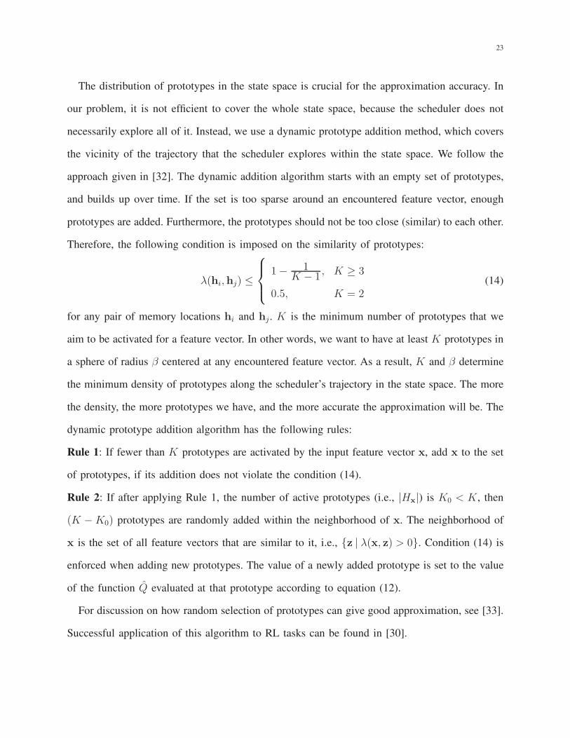
The distribution of prototypes in the state space is crucial for the approximation accuracy. In
our problem, it is not efficient to cover the whole state space, because the scheduler does not
necessarily explore all of it. Instead, we use a dynamic prototype addition method, which covers
the vicinity of the trajectory that the scheduler explores within the state space. We follow the
approach given in [32]. The dynamic addition algorithm starts with an empty set of prototypes,
and builds up over time. If the set is too sparse around an encountered feature vector, enough
prototypes are added. Furthermore, the prototypes should not be too close (similar) to each other.
Therefore, the following condition is imposed on the similarity of prototypes:
λ(hi,hj) ≤
1− 1K − 1 , K ≥ 3
0.5, K = 2(14)
for any pair of memory locations hi and hj. K is the minimum number of prototypes that we
aim to be activated for a feature vector. In other words, we want to have at least K prototypes in
a sphere of radius β centered at any encountered feature vector. As a result, K and β determine
the minimum density of prototypes along the scheduler’s trajectory in the state space. The more
the density, the more prototypes we have, and the more accurate the approximation will be. The
dynamic prototype addition algorithm has the following rules:
Rule 1: If fewer than K prototypes are activated by the input feature vector x, add x to the set
of prototypes, if its addition does not violate the condition (14).
Rule 2: If after applying Rule 1, the number of active prototypes (i.e., |Hx|) is K0 < K, then
(K −K0) prototypes are randomly added within the neighborhood of x. The neighborhood of
x is the set of all feature vectors that are similar to it, i.e., z | λ(x, z) > 0. Condition (14) is
enforced when adding new prototypes. The value of a newly added prototype is set to the value
of the function Q evaluated at that prototype according to equation (12).
For discussion on how random selection of prototypes can give good approximation, see [33].
Successful application of this algorithm to RL tasks can be found in [30].
24
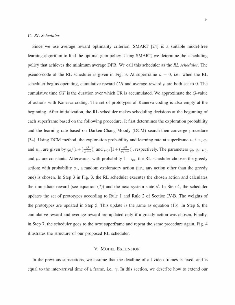
C. RL Scheduler
Since we use average reward optimality criterion, SMART [24] is a suitable model-free
learning algorithm to find the optimal gain policy. Using SMART, we determine the scheduling
policy that achieves the minimum average DFR. We call this scheduler as the RL scheduler. The
pseudo-code of the RL scheduler is given in Fig. 3. At superframe n = 0, i.e., when the RL
scheduler begins operating, cumulative reward CR and average reward ρ are both set to 0. The
cumulative time CT is the duration over which CR is accumulated. We approximate the Q-value
of actions with Kanerva coding. The set of prototypes of Kanerva coding is also empty at the
beginning. After initialization, the RL scheduler makes scheduling decisions at the beginning of
each superframe based on the following procedure. It first determines the exploration probability
and the learning rate based on Darken-Chang-Moody (DCM) search-then-converge procedure
[34]. Using DCM method, the exploration probability and learning rate at superframe n, i.e., qn
and µn, are given by q0/[1+( n2
qr+n)] and µ0/[1+( n2
µr+n)], respectively. The parameters q0, qr, µ0,
and µr are constants. Afterwards, with probability 1− qn, the RL scheduler chooses the greedy
action; with probability qn, a random exploratory action (i.e., any action other than the greedy
one) is chosen. In Step 3 in Fig. 3, the RL scheduler executes the chosen action and calculates
the immediate reward (see equation (7)) and the next system state s′. In Step 4, the scheduler
updates the set of prototypes according to Rule 1 and Rule 2 of Section IV-B. The weights of
the prototypes are updated in Step 5. This update is the same as equation (13). In Step 6, the
cumulative reward and average reward are updated only if a greedy action was chosen. Finally,
in Step 7, the scheduler goes to the next superframe and repeat the same procedure again. Fig. 4
illustrates the structure of our proposed RL scheduler.
V. MODEL EXTENSION
In the previous subsections, we assume that the deadline of all video frames is fixed, and is
equal to the inter-arrival time of a frame, i.e., γ. In this section, we describe how to extend our

25
proposed model and relax the fixed deadline assumption. We consider the general case where
the deadline for each flow i is equal to Γi ≥ γ. In particular, we assume that:
Γi = Jiγ, ∀Ji ∈ 1, 2, . . ., i = 1, . . . , F. (15)
Clearly, this require the queue of flow i needs to hold up to Ji frames. To incorporate the
extended deadline model in (15) into our problem formulation, we need to modify the state,
action, and reward models in our RL scheduler design. First, consider the set of system states
in (1). If (15) holds, then set S becomes:
S ,
s = (l,d, g, δ) | ∀ i ∈ F , 1 ≤ j ≤ Ji, 0 ≤ li,j ≤ txi(Lmaxi ),
di,j ∈ 0, . . . , Dmaxi , gi,j ∈ 0, . . . , Ni − 1, δi,j ∈ 0, 1
. (16)
Here l , [l1,1 · · · l1,J1lF,1 · · · lF,JF
], where li,j denotes the channel time required by the j th frame
in the queue of flow i, in milliseconds. the vectors d, g, and δ can be obtained similarly. On
the other hand, the value Dmaxi , ⌊Γi
η⌋ = ⌊γJi
η⌋, is the maximum frame deadline in units of
superframe size η.
Similarly, we can extend the set of all possible actions to be as follows:
A =
a , (a1,1, · · · aF,JF, p, q) | p ∈ F ∩ 0; 1 ≤ q ≤ Ji ai,j ∈ 0, 1, ∀ i ∈ F ,
j ∈ 1, . . . , Ji; apq = 0 if p 6= 0
, (17)
where aij is equal to 1 if the scheduler allocates enough channel time to flow i so that it can
fully transmit its j th frame. Given the action set A, at each epoch, the extended scheduler should
choose an action depending on the current state. Clearly, the channel time required to transmit
all scheduled frames for all flows should not exceed the length of the superframe. This requires
replacing (3) with the following extended constraint:
F∑
i=1
Ji∑
j=1
(ai,j · li,j) ≤ η. (18)

26
We notice that if Γi = γ for all flows i = 1, . . . , F , then the constraint in (18) simply reduces
to (3). After transmitting all the scheduled frames, the remaining time can be calculated as:
lpartial = η −F∑
i=1
Ji∑
j=1
(ai,j · li,j) ≤ η. (19)
Next, consider the reward model. We can write the state-dependent cost function as follows:
ci,j(s) =
(
Ni + (Mi − 1))
· ei,j · Udi,j=1, if yi(gi,j) = I,
ei,j · Udi,j=1, if yi(gi,j) = B,(
Ni − 1− (gi,j
Mi− 1)Mi
)
· ei,j · Udi,j=1, if yi(gi,j) = P .
(20)
Note that yi( ), Mi and Ni do not have j index because they are indeed defined in per flow
basis. We can also extend the reward function to be as follows:
r(s(n), a(n)) =F∑
i=1
Ji∑
j=1
[
ai,j(n)− ci,j(s(n))(1− ai,j(n))
]
. (21)
Given the reward function above, we can rewrite the policy gain to be:
ρπ =1
T
T∑
n=1
r(s(n), a(n))
=
F∑
i=1
(
∑Tn=1
∑Ji
j=1 ai,j(n)−∑T
n=1
∑Ji
j=1 ci,j(s(n))(1− ai,j(n))
T
)
. (22)
In this case, the total number of frames for each flow is total frames = total timeinter arrival time
= ηT
γ.
Furthermore, the terms∑T
n=1
∑Ji
j=1 ai,j(n) and∑T
n=1
∑Ji
j=1 ci,j(s(n))(1− ai(n)) in (22) are in
fact the total number of scheduled frames and the total number of undecodable frames for each
flow, respectively. In addition, these two terms sum up to the total number of frames for flow
i. Consequently, after reordering the terms, the policy gain in (22) becomes exactly the same
as that in (9). Therefore, (10) also still holds and an optimal (maximum) gain policy yields the
optimal (minimum) average DFR, which is what we aim to find in presence of the extended
model.
Next, we extend the state transitions model to the general case when the deadline Γi for flow i
is as in (15). At superframe n, the system is in state s(n) and chooses the action a(n). The next
27
state s(n + 1) depends on s(n), a(n) and new frame arrivals. We determine the state transitions
per flow, i.e., we show how the state variables relate to each flow change. The whole system
state is updated by performing the same procedure for all the flows.
When di,1(n) ≥ 1, no new video frame will arrive for flow i. Thus, the remaining time until
the next arrival is reduced by one superframe. If any frame of a flow is scheduled, its length
will become 0. And if it is partially transmitted, its length will reduce by lpartial. Otherwise,
the length remains unchanged. The frame offset within GOP also does not change. The value
of δi,j changes only when an I or P frame of flow i expires, or when a new GOP starts, which
is indicated by arrival of a new I frame for flow i. None of these happens when di,1(n) ≥ 1.
Hence, if di,1(n) ≥ 1, then for each j ∈ 1 . . . Ji, the state deterministically changes as follows:
di,j(n + 1) = di,j(n)− 1, (23)
li,j(n + 1) = li,j(n)(1− ai,j(n))− lpartialUi=p and j=q, (24)
gi,j(n + 1) = gi,j(n), (25)
δi,j(n + 1) = δi,j(n). (26)
When di,1(n) = 0, it means that the first frame in the queue of flow i has expired, if it has
not already been sent, i.e., if li,1(n) 6= 0. It also means that a new frame will arrive for flow i,
within superframe n. We shift the frames in the queue (getting rid of the head frame) and add
the new frame to the tail of the queue. We denote the deadline and channel time requirement of
the newly arrived frame for flow i within superframe n by dnewi (n) and lnew
i (n), respectively.
Let probi(lnewi (n)) denote the probability that the channel time request of flow i is lnew
i (n).
Thus, when di,1(n) = 0 ,the state changes with probability probi(lnewi (n)) as follows:
di,Ji(n + 1) = dnew
i (n), (27)
li,Ji(n + 1) = lnew
i (n), (28)
gi,Ji(n + 1) = (gi,Ji
(n) + 1) mod Ni. (29)

28
We notice that the exact model for δi,J(n + 1) depends on the considered scenario. It is very
difficult (if possible) to provide a general closed-form model for δi,J(n+1) for extended deadline
model. On the other hand, for each j ∈ 2, · · · , J we have:
di,j−1(n + 1) = di,j(n), (30)
li,j−1(n + 1) = li,j(n), (31)
gi,j−1(n + 1) = gi,j(n), (32)
δi,j−1(n + 1) = δi,j(n). (33)
Given the extended models in (15)-(33), our proposed RL algorithm can be used to obtain the
optimal solutions for the general case when the deadlines are indeed arbitrarily for each flow.
VI. PERFORMANCE EVALUATION AND COMPARISONS
In this section, we evaluate the performance of our proposed scheduling algorithm. We use the
real MPEG-4 trace of Jurassic Park movie with GOP pattern of (N = 12, M = 3) [35]. The frame
rate is 30 frames per second. The average rate of each flow is 8 Mbps. In the simulation model,
each iteration (i.e., simulation run) lasts 500 s. The superframe size is η = 8 ms; thus, each
iteration consists of 500/0.008 = 62, 500 superframes (i.e., decision epochs). The parameters p0
and µ0 of the DCM scheme algorithm depend on how fast the scheduler can learn the optimal
policy. We set p0 = µ0 = 0.1 and pr = µr = 1010, as it gives the RL scheduler enough time to
explore and find the optimal policy without too many iterations. We end the simulation when
both the learning rate and exploration probability fall below 0.005.
The rest of the simulation parameters are as follows. The channel data rate is 100 Mbps,
the number of MPEG-4 flows varies from 2 to 10. The maximum tolerable delay for MPEG-4
frames is 1/30 s and maximum MAC fragment size is 2048 bytes. We use the average DFR as
the performance metric. For F-SRPT [5], EDD+SRPT [6], and PAP [2] scheduling algorithms
we use the performance that is already improved by the FDA technique described in [13].

29
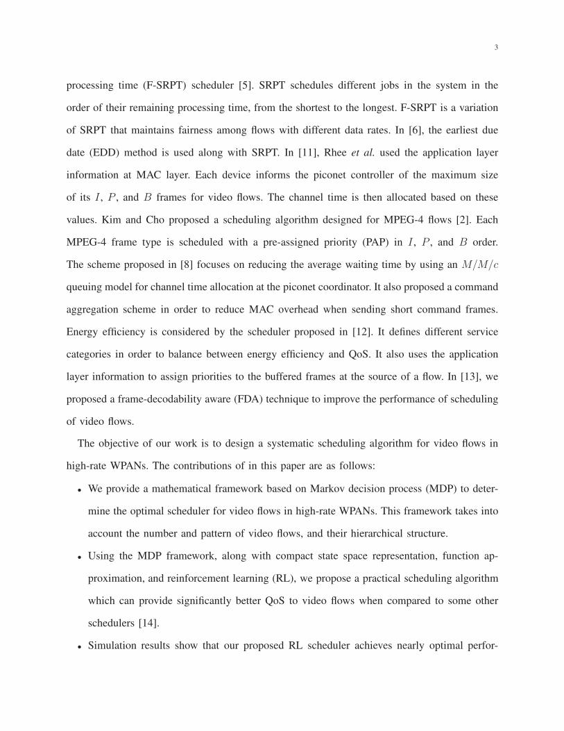
Fig. 5 compares the average DFR achieved by RL, EDD+SRPT, PAP, and F-SRPT algorithms
when the number of MPEG-4 flows varies from 2 to 10. We see that RL scheduler performs better
than the others regardless of the number of MPEG-4 flows. The relative reduction of average
DFR is up to 42%, 49%, and 53% for EDD+SRPT, PAP, and F-SRPT scheduler, respectively.
The start time of different flows in the system affects the burstiness of traffic load, and thus
influences the overall performance. In order to show this fact, we assume that the start times of
flows are separated by φ seconds. In other words, flow i starts at time iφ [5]. Fig. 6 compares
the average DFR achieved by RL, F-SRPT, EDD+SRPT, and PAP scheduling algorithms when
φ varies from 1 to 30 ms. The number of MPEG-4 flows is equal to 9. We can see that our
proposed RL scheduler performs better than the other three for all values of φ. Furthermore, the
performance of RL scheduler is less sensitive to φ.
To evaluate the optimality of the RL algorithm, we consider the special case of interest which
is when φ = 0, i.e., when all the flows in the system start at the same time. In [14], we show
that for this case, the SRPT scheduler is the optimal scheduler. Fig. 7 compares the average
DFR achieved by RL algorithm with the optimal case when the number of MPEG-4 flows varies
from 2 to 10. We can see that in all cases, RL scheduler provides nearly optimal performance.
Table III shows that reduction of the average DFR can also be translated to system capacity
enhancement. Suppose that the acceptable user perceived quality is equivalent to the average DFR
being less than 5%. Thus, the capacity of the system can be defined as the number of video
flows that can be admitted to the system, while the average DFR is less than the maximum
allowable value of 5%. Using this definition, the system capacity is 7 flows for the conventional
schedulers, as opposed to 8 flows for the RL scheduler. Consequently, in this example, the RL
scheduler increases the system capacity by 14.3%.
As mentioned in Section III, the policy gain and DFR have a linear relationship. We can
verify the validity of equation (10) as follows. First, the estimated average DFR is calculated by
substituting the policy gain ρ in equation (10). Second, the exact average DFR is measured by

30
counting the number of scheduled frames. Fig. 8 compares these two values. As one can see,
DFR in equation (10) under-estimates the exact average DFR, because the gain is only updated
when the scheduler takes a greedy action. However, both greedy and exploratory actions affect
the exact average DFR. Over time, with more iterations, as the RL scheduler learns the optimal
policy and the exploration probability decays, the exact and estimated average DFR converge
together. This result verifies that the optimal gain policy yields the minimum average DFR.
VII. CONCLUSIONS AND FUTURE WORK
In this paper, we formulated the scheduling of video flows in high-rate WPANs as an MDP
problem. This model incorporates the decodability information extracted by the FDA technique.
It also takes into account the number and pattern of video flows, and their hierarchical structure.
The solution to this MDP problem is the optimal scheduling policy that minimizes the average
DFR. Using compact state space representation and function approximation, we simplified the
MDP problem in order to solve it with RL. Our proposed RL scheduler is the solution given by
an RL technique called SMART. Simulation results showed that when FDA technique is applied
to the F-SRPT and EDD+SRPT schedulers, there are up to 61% and 60% reduction in DFR,
respectively. Results also showed that the RL scheduler reduces the average DFR by 42%, 49%,
and 53% when compared to EDD+SRPT, PAP, and F-SRPT schedulers, respectively.
With the variety of applications that a high-rate WPAN should be able to support, it will
serve different classes of traffic with different QoS requirements. We focused on the video
traffic class in this paper. Therefore, extending the RL scheduler which can handle and recognize
different traffic types is part of our work. This is possible by defining proper reward function
and modifying the state space model. In the new setting, the scheduler can be designed to
achieve the best overall performance based on a combination of different rewards and costs.
Moreover, the issue of fairness among the scheduled video flows is also a critical point, which
is not considered in this paper. Another direction for future work is to account for fairness by

31
formulating the problem as an MDP with constraints that enforce the fairness criterion. Using
fuzzy logic for function approximation can also be of interest. Furthermore, it is possible to
accommodate more flows into the system if we can take concurrent transmissions into account
using time domain spreading (TDS) as well as frequency domain spreading (FDS) techniques.
Finally, it is possible to extend our model to incorporate the impact of jitter by framing the
arrival time probabilistically, rather than deterministically.
ACKNOWLEDGMENT
This work is supported by Bell Canada and the Natural Sciences and Engineering Research
Council of Canada (NSERC).
REFERENCES
[1] “IEEE Std 802.15.3-2003: Wireless medium access control (MAC) and physical layer (PHY) specifications for high rate
wireless personal area networks (WPANs),” Sept. 2003.
[2] S. M. Kim and Y. J. Cho, “Scheduling scheme for providing QoS to real-time multimedia traffics in high-rate wireless
PANs,” IEEE Transactions on Consumer Electronics, vol. 51, no. 4, pp. 1159–1168, Nov. 2005.
[3] X. Shen, W. Zhuang, H. Jiang, and J. Cai, “Medium access control in ultra-wideband wireless networks,” IEEE Transactions
on Vehicular Technology, vol. 54, no. 5, pp. 1663–1677, Sept. 2005.
[4] C. Hu, H. Kim, J. Hou, D. Chi, and S. Shankar, “Provisioning quality controlled medium access in UWB-operated WPANs,”
in Proc. of IEEE Infocom, Barcelona, Spain, Apr. 2006.
[5] R. Mangharam, M. Demirhan, R. Rajkumar, and D. Raychaudhuri, “Size matters: size-based scheduling for MPEG-4 over
wireless channels,” in Proc. of SPIE/ACM Multimedia Computing and Networking (MMCN), Santa Clara, CA, Jan. 2004,
pp. 110–122.
[6] A. Torok, L. Vajda, A. Vidacs, and R. Vida, “Techniques to improve scheduling performance in IEEE 802.15.3 based ad
hoc networks,” in Proc. of IEEE Globecom, St. Louis, MO, Nov. 2005.
[7] Y. C. Chu and A. Ganz, “Joint scheduling and resource control for QoS support in UWB-based wireless networks,” in
Proc. of IEEE Military Communications Conference (MILCOM), Monterey, CA, Nov. 2004, pp. 1100–1106.
[8] R. Zeng and G. S. Kuo, “A novel scheduling scheme and MAC enhancements for IEEE 802.15.3 high-rate WPAN,”
in Proc. of IEEE Wireless Communications and Networking Conference (WCNC), New Orleans, CA, Mar. 2005, pp.
2478–2483.

32
[9] C. Y. Zou and Z. Haas, “Optimal resource allocation for UWB wireless ad hoc networks,” in Proc. of IEEE 16th
International Symposium on Personal, Indoor and Mobile Radio Communications (PIMRC), Berlin, Germany, Sept. 2005,
pp. 452–456.
[10] K. H. Liu, L. Cai, and X. Shen, “Performance enhancement of medium access control for UWB WPAN,” in Proc. of IEEE
Global Telecommunications Conference (GLOBECOM), San Francisco, CA, Nov. 2006.
[11] S. H. Rhee, K. Chung, Y. Kim, W. Yoon, and K. S. Chang, “An application-aware MAC scheme for IEEE 802.15.3
high-rate WPAN,” in Proc. of IEEE Wireless Communications and Networking Conference (WCNC), Atlanta, GA, Mar.
2004, pp. 1018–1023.
[12] X. Chen, Y. Xiao, Y. Cai, J. Lu, and Z. Zhou, “An energy Diffserv and application-aware MAC layer scheduling for multiple
VBR video streaming over high-rate WPANs,” Elsevier Computer Communications, vol. 29, no. 17, pp. 3516–3526, Nov.
2006.
[13] S. Moradi and V. W. S. Wong, “Technique to improve MPEG-4 traffic schedulers in IEEE 802.15.3 WPANs,” in Proc. of
IEEE International Conference on Communications (ICC), Glasgow, Scotland, June 2007.
[14] S. Moradi, “A novel scheduling algorithm for video flows in high-rate WPANs,” Master’s thesis, University of British
Columbia, Vancouver, Canada, Apr. 2007. [Online]. Available: http://www.ece.ubc.ca/∼vincentw/T/moradi.pdf
[15] S. Moradi, A. H. Mohsenian-Rad, and V. W. S. Wong, “A novel scheduling algorithm for video traffic in high-rate WPANs,,”
in Proc. of IEEE Global Telecommunications Conference (Globecom), Washington, DC, Dec. 2007.
[16] “MPEG-4 part 2: Visual (IS 14496-2), doc. N2502,” Oct. 1998.
[17] A. Ziviani, B. E. Wolfinger, J. F. Rezende, O. C. Duarte, and S. Fdida, “Joint adoption of QoS schemes for MPEG streams,”
Multimedia Tools and Applications, vol. 26, no. 1, pp. 59–80, May 2005.
[18] L. Schrage, “Proof of the optimality of the shortest remaining processing time discipline,” Operations Research, vol. 16,
pp. 678–690, 1968.
[19] S. S. Panwar, D. Towsley, and J. K. Wolf, “Optimal scheduling policies for a class of queues with customer deadlines to
the beginning of service,” Journal of the ACM, vol. 35, no. 4, pp. 832–844, 1988.
[20] L. P. Kaelbling, M. L. Littman, and A. P. Moore, “Reinforcement learning: A survey,” Journal of Artificial Intelligence
Research, vol. 4, pp. 237–285, 1996.
[21] R. S. Sutton and A. G. Barto, Reinforcement Learning: An Introduction. Cambridge, MA: MIT Press, 1998.
[22] A. Gosavi, “Reinforcement learning for long-run average cost,” European Journal of Operational Research, vol. 155, pp.
654–674, 2004.
[23] F. Yu, V. Wong, and V. Leung, “A new QoS provisioning method for adaptive multimedia in cellular wireless networks,”
in Proc. of IEEE Infocom, Hong Kong, China, Mar. 2004, pp. 2130–2141.
[24] T. K. Das, A. Gosavi, S. Mahadevan, and N. Marchalleck, “Solving semi-Markov decision problems using average reward
reinforcement learning,” Journal of Management Science, vol. 45, no. 4, pp. 560–574, 1999.

33
[25] A. Gosavi, “An algorithm for solving semi-markov decision problems using reinforcement learning: convergence analysis
and numerical results,” Ph.D. dissertation, University of South Florida, 1999.
[26] A. Gosavi, N. Bandla, and T. K. Das, “A reinforcement learning approach to a single leg airline revenue management
problem with multiple fare classes and overbooking,” IIE Transactions, vol. 34, pp. 729–742, 2002.
[27] M. L. Puterman, Markov decision processes: discrete stochastic dynamic programming. Wiley-Interscience, 1994.
[28] J. M. Gimenez-Guzman, J. Martinez-Bauset, and V. Pla, “An afterstates reinforcement learning approach to optimize
admission control in mobile cellular networks,” Lecture Notes in Computer Science: Wireless Systems and Network
Architectures in Next Generation Internet, vol. 3883, pp. 115–129, 2006.
[29] P. Kanerva, Sparse distributed memory. Cambridge, MA: MIT Press, 1988.
[30] B. Ratitch, S. Mahadevan, and D. Precup, “Sparse distributed memories in reinforcement learning: Case studies,” in Proc. of
the Workshop on Learning and Planning in Markov Processes - Advances and Challenges, San Jose, CA, July 2004, pp.
85–90.
[31] K. Kostiadis and H. Hu, “KaBaGe-RL: Kanerva-based generalisation and reinforcement learning for possession football,”
in Proc. of IEEE/RSJ International Conference on Intelligent Robots and Systems, Maui, HI, Nov. 2001, pp. 292–297.
[32] B. Ratitch and D. Precup, “Sparse distributed memories for on-line value-based reinforcement learning,” in Proc. of the
European Conference on Machine Learning (ECML), Pisa, Italy, Sept. 2004, pp. 347–358.
[33] R. S. Sutton and S. D. Whitehead, “Online learning with random representations,” in Proc. of the International Conference
on Machine Learning, Amherst, MA, June 1993, pp. 314–321.
[34] C. Darken, J. Chang, and J. Moody, “Learning rate schedules for faster stochastic gradient search,” in Proc. of IEEE
Workshop on Neural Networks for Signal Processing, Copenhagen, Denmark, Sept. 1992.
[35] F. Fitzek and M. Reisslein, “MPEG-4 and H.263 video traces for network performance evaluation,” IEEE Network, vol. 15,
pp. 40–54, Nov./Dec. 2001.
34
Fig. 1. Superframe structure. The presence of CAP is optional. The number, duration and order of the CTAs and MCTAs can
vary from one superframe to another.
Fig. 2. GOP structure (N = 9, M = 3). The arrows indicate the direction of decoding dependencies.
35
TABLE I
LIST OF NOMENCLATURE.
Notation Parameter definition
A Action set in MDP model.
a Action vector in MDP model.
ai Binary action for flow i.
B Bidirectional frame.
Dmax maximum frame deadline in units of superframe size η.
di Number of full superframes left until the arrival of the next frame.
ei A binary variable to denote the eligibility of flow i being scheduled.
F Number of video flows.
F Set of video flows.
gi Offset of the frame in the queue of flow i, with respect to the beginning of the frame’s GOP.
hk The kth prototype in Kanerva coding.
I Intra-coded frame.
Lmaxi
Maximum frame size of flow i.
li Channel time required by the frame in the queue of flow i, in milliseconds.
lpartial Remaining channel time.
Mi I-to-P frame distance of the ith video flow.
Ni I-to-I frame distance of the ith video flow.
P Predictive frame.
p The flow which can only transmit parts of its frame during a scheduling period.
S State space in MDP model.
s State vector in MDP model.
Ω Set of feature vectors.
β Activation radius in Kanerva coding.
δi Binary variable for flow i.
η Size of a superframe.
γ Inter-arrival time.
λ( ) Similarity function.
ρπ Policy gain given the use of policy π.
txi(x) Channel time that flow i requires to send x bits of data.

36
TABLE II
NUMBER OF FRAME DEPENDENCIES FOR EACH VIDEO FRAME
Frame type Number of frames
I N + (M − 1)
Pk, k = 1, . . . , N
M− 1 N − 1 − (k − 1)M
B 1
TABLE III
QUANTITATIVE COMPARISON AMONG RL SCHEDULER AND CONVENTIONAL SCHEDULERS. THE MINIMUM AVERAGE DFR
GIVEN BY F-SRPT, EDD+SRPT, AND PAP IS USED FOR COMPARISON.
Number of Flows F 6 7 8 9 10
Minimum Average DFR (%) 1.5 4.0 7.2 10.7 14.4
RL Average DFR (%) 0.9 2.3 4.4 7.2 10.5
Absolute Reduction (%) 0.6 1.7 2.8 3.4 3.9
Relative Reduction (%) 42 42 38 32 27

37
Initialize the superframe number n = 0, cumulative reward CR = 0, cumulative time CT = 0, and the average
reward ρ = 0. In addition, the set of prototypes is initialized as the empty set. The Superframe size is η.
Suppose that the system starts in state s.
while n < MAX STEPS do
1) Calculate exploration probability qn and learning rate µn using the DCM method.
2) With probability 1−qn, choose the greedy action a ∈ As that maximizes Q(f(s,a)); otherwise, choose
a random exploratory action from the set As \ a.
3) Execute the chosen action. Let the system state at the next superframe be s′, and the immediate received
reward be r(s,a).
4) Apply Rule 1 and Rule 2 of Section IV-B to the feature vector x = f(s,a).
5) Update the weight of the prototypes according to:
wi ← wi + µn
λi∑
k∈Hx
λk
[
r(s,a) − ηρ + maxa′
Q(f(s′,a′))]
− Q(f(s,a))
, ∀i ∈ Hx
6) if a greedy action was chosen in Step 2, then
Update CT ← CT + η;
Update CR← CR + r(s,a) and ρ← CR/CT ;
else go to Step (2).
7) Go to the next superframe, i.e., update n← n + 1 and s← s′.
Fig. 3. Pseudo-code of the RL scheduler.
Fig. 4. Structure of the RL scheduler.

38
2 3 4 5 6 7 8 9 100
0.05
0.1
0.15
0.2
Number of MPEG−4 Flows
Ave
rag
e D
FR
PAP with FDAF−SRPT with FDAEDD+SRPT with FDARL
Fig. 5. Comparison of RL scheduler and other schedulers when the number of video flows varies from 2 to 10.
0 5 10 15 20 25 300
0.1
0.2
0.3
0.4
0.5
0.6
0.7
0.8
Time Separation [ms]
Ave
rag
e D
FR
PAP with FDAF−SRPT with FDAEDD+SRPT with FDARL
Fig. 6. Effect of time separation on average DFR. The RL scheduler has the smallest average DFR for all φ.

39
2 3 4 5 6 7 8 9 100
0.1
0.2
0.3
0.4
0.5
0.6
Number of MPEG−4 Flows
Ave
rag
e D
FR
Optimal SchedulerRL Scheduler
Fig. 7. Comparison of RL scheduler and optimal scheduler for φ = 0. RL scheduler is nearly optimal in this case.
1 2 3 4 5 6 7 8 9 10 11 12 13 14 15 160.06
0.065
0.07
0.075
0.08
0.085
Iteration Number
Avera
ge D
FR
Exact Average DFREstimated Average DFR
Fig. 8. Comparison of the exact and estimated DFR (F = 9).