Optimal Trafﬁc Scheduling for Intrusion Prevention Systems

Optimal Traffic Scheduling forIntrusionPrevention Systems

J. Crichigno1∗, M. Pourvali2, F. Shaikh2, A. Rayes3, E. Bou-Harb4, N. Ghani2

Abstract—A major challenge for intrusion prevention system(IPS) sensors in today’s Internet is the amount of traffic thesedevices have to inspect. Hence this paper presents a linearprogram (LP) for traffic scheduling in multi-sensor environmentsthat alleviates inspection loads at IPS sensors. The model discrim-inates traffic flows so that the amount of inspected suspicioustraffic is maximized. While the LP is not constrained to integralsolutions, traffic belonging to a flow is mostly scheduled for in-spection to a single sensor, which facilitates the collection of stateinformation. An analysis of how the Simplex algorithm solves themodel and numerical results demonstrate that state informationcan be preserved without imposing integral constraints. Thisbenefit prevents the LP from becoming an integer linear program(ILP), which is essential for efficiently implementing the proposedmodel. The paper also shows that the ratio of the total number offlows integrally inspected by a single sensor to the total numberof flows inspected in a multi-sensor environment depends on theratio of IPS sensor capacity to flow traffic rate. Finally, somepractical deployment observations are presented.

Keywords—IPS, Linear Programming, Computer Networks.

I. I NTRODUCTION

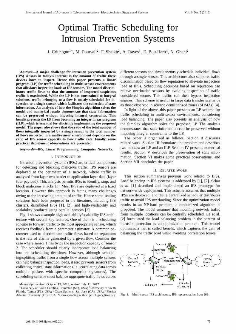
Intrusion prevention systems (IPSs) are critical componentsfor detecting and blocking malicious traffic. IPS sensors aredeployed at the perimeter of a network, where traffic isanalyzed from layer two header to application layer data (layerfour payload). This analysis permits IPSs to identify, stop, andblock malicious attacks [1]. Most IPSs are deployed at a fixedlocation. However this approach is facing many challengesowing to the increasing amount of traffic. Hence some scalingsolutions have been proposed in the literature, including IPSclusters, distributed IPSs [1], [2], and high-availability andscalability products using parallel sensors [3].

Fig. 1 shows a sample high-availability/scalability IPS archi-tecture with several key features. One of them is a schedulingscheme to forward traffic to the most appropriate sensor, whichreceives feedback from a parameter estimator. A common pa-rameter used to discriminate traffic flows based on reputationis the rate of alarms generated by a given flow. Consider thecase where sensor 1 has twice the inspection capacity of sensor2. The scheduler should clearly incorporate load balancinginto the scheduling decisions. However, although schedul-ing/splitting traffic from a single flow across multiple sensorscan help balance inspection loads, it also prevents sensors fromcollecting critical state information (i.e., correlating data acrossmultiple packets with specific composite signatures). Thescheduling scheme must balanceaggregate traffic flows across

Manuscript received October 13, 2016, revised July 11, 2017.1University of South Carolina, Columbia (SC), USA;2University of South

Florida, Tampa (FL), USA;3Cisco Systems, San Jose (CA), USA;4FloridaAtlantic University (FL), USA.∗Corresponding author: [email protected]

different sensors and simultaneously schedule individual flowsthrough a single sensor. This architecture also supports trafficdiscrimination based on flow reputation to alleviate inspectionload at IPSs. Scheduling decisions based on reputation canrelieve overloaded sensors by avoiding inspection of trafficconsidered secure. This traffic can then bypass inspectionengines. This scheme is useful in large data transfer scenariosas those observed in science demilitarized zones (SDMZs) [4].

In light of the above, this paper presents an LP scheme fortraffic scheduling in multi-sensor environments, consideringload balancing. The paper also presents an analysis of howthe Simplex algorithm solve the proposed LP. The analysisdemonstrates that state information can be preserved withoutimposing integral constraints to the LP.

The paper is organized as follows. Section II discussesrelated work. Section III formulates the problem and describestwo models: an LP and an ILP. Section IV presents numericalresults. Section V describes the preservation of state infor-mation. Section VI makes some practical observations, andSection VII concludes the paper.

II. RELATED WORK

This section summarizes previous work related to IPSs.Load balancing in IPS systems is addressed by [1], [2]. Sekaret al. [1] described and implemented an IPS prototype fornetwork-wide deployment. This scheme assumes that multipleIPSs are deployed, and that a centralized scheduler distributestraffic to avoid IPS overloading. Since the optimization modelresults in an NP-hard problem, a randomized algorithm isproposed. The model assumes that incoming network trafficfrom multiple locations can be centrally scheduled. Le et al.[2] formulated the load balancing problem in the context ofintrusion detection as an optimization problem. This modeloptimizes a metric called benefit, which captures the gain ofbalancing the traffic load while avoiding correlation losses.

Fig. 1. Multi-sensor IPS architecture. IPS representation from [6].

doi: 10.11601/ijates.v6i2.201

International Journal of Advances in Telecommunications, Electrotechnics, Signals and Systems Vol. 6, No. 2 (2017)

73

Commercial IPSs also deploy high-availability and scala-bility products which use parallel sensors to avoid the typicalsingle point of failure. Other related works for scaling IDS/IPSuse parallelization [7],[8],[9]. These schemes exploit the com-putational power of supercomputers (or multi-core computers)by adopting a parallel architecture combining data and pipelineparallelism [7]. Zhanget al. [10] proposed an SDN-basedIPS deployment that supports unified scheduling of securityapplications in the whole network (and also load balancingamong IPSs). Laniepceet al. [11] highlighted the challengesassociated with designing intrusion monitoring and preventionservices in the cloud. Finally, Xinget al. [12] used OpenFlowand Snort to build an IPS called SnortFlow. This system canbe reconfigured on-the-fly based on dynamic conditions.

III. PROBLEM FORMULATION

This section is organized as follows. Section III-A presentsan LP for traffic scheduling in multi-sensor environments.Section III-B incorporates integral constraints to the previouslydefined LP and presents the resulting ILP, and Section III-Cdiscusses the complexity of both LP and ILP models.

A. Linear Program (LP) model

Let S be the set of sensors or IPSs. Each sensors ∈ S

has a processing capacitycs, measured in traffic units (e.g.pps, Mbps, Gbps). LetN be the set of traffic flows to beinspected by the sensors. A flow is defined as a 5-tuple givenby {source IP address, source port, destination IP address,destination port, traffic rate}. The latter is denoted byrn,n ∈ N . Let An be the total number of traffic units of flown ∈ N that triggered alarm events. An alarm event is raisedwhen a signature is examined against an event (e.g. a packet),and a match is found between the signature and the event(i.e. potential security violation). The proposed model uses adimensionless metric defined as thealarm rate to estimate therate at which suspicious events occur in flown. This metricis given by the following ratio:

pn =An

rn. (1)

where0 ≤ pn ≤ 1. If the traffic rn does not raise any alarm,pn = 0. If all traffic rn generates alarms,pn = 1.

Let xn,s be the fraction of traffic from flown ∈ N to bescheduled at sensors ∈ S. If all traffic rn is successfullyscheduled and inspected by sensors, then

∑

s∈S xn,s = 1. Let0 ≤ α ≤ 1 be the maximum utilization among all sensors.Note that a similar metric is also used in IP networks for loadbalancing [13]. A value ofα = 1 means that at least one sensoris operating at full capacity. Based on the above definitions,the proposed LP is defined by:

Max F = w1

∑

n∈N

∑

s∈S

pnrnxn,s − w2α. (2)

∑

s∈S

xn,s ≤ 1 n ∈ N. (3)

∑

n∈N

rnxn,s ≤ csα s ∈ S. (4)

xn,s ≥ 0 n ∈ N, s ∈ S. (5)

0 ≤ α ≤ 1. (6)

The objective function of the LP, referred as LP-IPS in therest of the paper, consists of two terms with weightsw1 andw2. The first term is the summation of all traffic inspectedby all sensors, multiplied by their corresponding alarm rates.SinceF is maximized, the linear program prioritizes flowswith high alarm rates. Forn ∈ N , the term

∑

s∈S pnrnxn,s

can be considered as suspicious traffic. Thus, the first term ofEq. (2) is the aggregated expected suspicious traffic (EST):

EST =∑

n∈N

∑

s∈S

pnrnxn,s. (7)

The second term in Eq. (2) is the maximum utilization amongall sensors. Maximizing the negative ofα is equivalent tominimizing it. Constraint (3) states that the total fraction oftraffic from flown ∈ N inspected by all sensors should be lessor equal to unity. Constraint (4) limits the amount of trafficinspected by sensors ∈ S, where the inspection capacitycsis multiplied byα.

B. Integer Linear Program (ILP) Model

An atomic signature consists of a single event (e.g. packet)that is examined to determine if it matches a configured signa-ture. Since these signatures can be matched on a single event,they do not require a sensor to maintain state information.On the other hand, a composite signature requires severalpieces of data (e.g., packets) to match an attack signature, andhence a sensor must maintain state information. The LP-IPSmodel permits an individual traffic flow to be split and sched-uled across multiple sensors. However splitting traffic impliesthat sensors cannot collect full state information. Thereforeif composite signatures are predominant, maintaining stateinformation will be critical. As a result, all trafficrn of aflow n ∈ N may need to be routed through a single sensor.

The LP-IPS can be modified so that traffic from a singleflow n ∈ N is not split. This requirement can be added byrestricting variablesxn,s to be binary integers (0 or 1). Theassociated program is defined by:

Max F = w1

∑

n∈N

∑

s∈S

pnrnxn,s − w2α. (8)

∑

s∈S

xn,s ≤ 1 n ∈ N. (9)

∑

n∈N

rnxn,s ≤ csα s ∈ S. (10)

xn,s ∈ {0, 1} n ∈ N, s ∈ S. (11)

0 ≤ α ≤ 1. (12)

Note that restricting variables to take integral values convertsthe LP-IPS into an ILP. This ILP will be referred as ILP-IPS in the rest of the paper. Also, note that Constraint (9) iseither satisfied with equality when a single sensor is used toinspect the traffic of a flown ∈ N (i.e. only one variablexn,s

is unity), or satisfied with inequality when the traffic is notinspected by any sensor (i.e. all variablesxn,s are zero).


74

C. Complexity of LP-IPS

Since the LP-IPS is a linear program, it can be solved inpolynomial time in the size of the problem. The size of LP-IPS is given by the number of constraints and variables. From(5) and (6), the total number of variables isk = |N | · |S|+1.Similarly, from (3),(4),(5) and (6), the number of constraintsis m = |N | + |S| + |N | · |S| + 2. Both k and m arepolynomial in the number of variables and constraints. Inpractice the Simplex method runs in polynomial time ofk

and m. Similarly, the Interior Point method can solve LP-IPS problem in a polynomial time that is upper-bounded byO(k2m) [14]. On the other hand, the ILP-IPS problem isan integer linear program and is therefore NP-hard, i.e. therunning time is exponential in the size of the problem.

IV. I LLUSTRATIVE EXAMPLES

This section presents first a small illustrative example in adual-sensor scenario (Section IV-A), followed by a dynamicexample where traffic flows arrive one by one (Section IV-B).

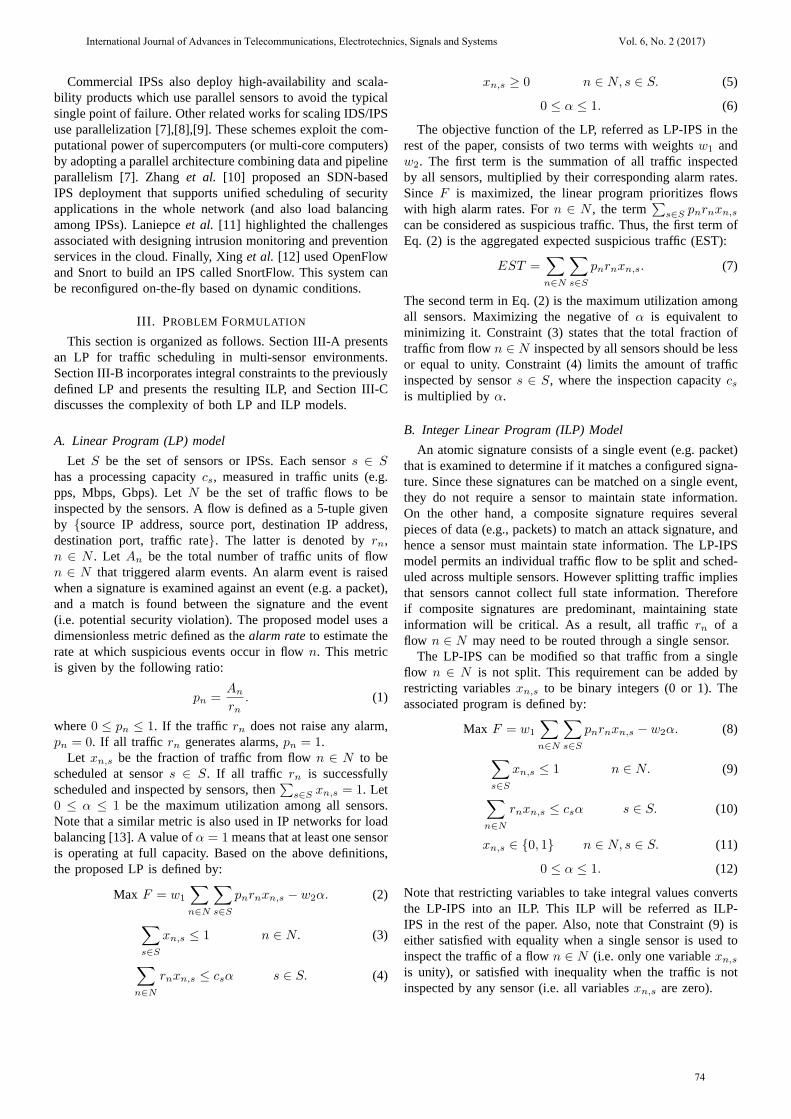
A. Illustrative Example 1: Dual-Sensor Scenario

Fig. 2(a) illustrates a scenario where sensorss0 ands1 haveinspection capacities ofc0 = 1000 andc1 = 1500 traffic units,respectively. These sensors have to inspect two traffic flows 0and 1, which are characterized by traffic and alarm ratesr0,p0, and r1, p1, respectively. Given that the aggregate trafficrate is less than the aggregate inspection capacity, the solutionfor the LP-IPS should perform load balancing. Similarly, ILP-IPS should also perform load balancing by scheduling flows0 and 1 through different sensors.

The solutions for the LP-IPS and ILP-IPS models are shownin Table I. The respective objective functions only differ in theα performance metric, while EST is the same. LP-IPS is ableto minimize the maximum utilization among the sensors toα = 0.64 by scheduling 80% of flow 1 via sensor 0 and theremainder of flow 1 and flow 0 through sensor 1. ILP-IPSschedules all traffic from flow 0 to sensors0, and traffic fromflow 1 to sensors1. This solution results in a utilization of 0.80and 0.53 for sensorss0 ands1, respectively. Thusα = 0.80.

Example 1 shows how load balancing can be achieved whenthe aggregate inspection capacity exceeds the aggregate trafficrate. The subsequent dynamic scenarios will show how LP-IPS discriminates traffic when aggregate inspection capacityis less that aggregate traffic rate.

B. Illustrative Example 2: Dynamic Scenarios

The second illustrative example presents two dynamic sce-narios where 1000 flows arrive in random sequential manner.Here the sensors must discriminate which flows are moreimportant to inspect, since the aggregate inspection capacity is

TABLE ISOLUTION FOR EXAMPLE 1

Scheme Solution α

LP-IPS x0,0 = 0.0, x0,1 = 1.0, x1,0 = 0.8, x1,1 = 0.2 0.64ILP-IPS x0,0 = 1.0, x0,1 = 0.0, x1,0 = 0.0, x1,1 = 1.0 0.80

Fig. 2. (a) Dual-sensor scenario, (b) single-sensor scenario.

less than the aggregate traffic rate. All flows are inspected by5 sensors with 100 traffic units of capacity each. Flow inter-arrival times are uniformly distributed between (1-60) timeunits and their durations are uniformly distributed from (1-15)time units. Alarm rates are also uniformly distributed between(0.0001-0.5). Two dynamic scenarios are tested. In scenario 1,the traffic rate is uniformly distributed between (1-50) trafficunits (expected value ofrn, n ∈ N, is E[rn] = 25.5). InScenario 2, the traffic rate is uniformly distributed between(1-10) traffic units (E[rn] = 5.5). Since the ILP-IPS is NP-hard, only the LP-IPS solution is shown.

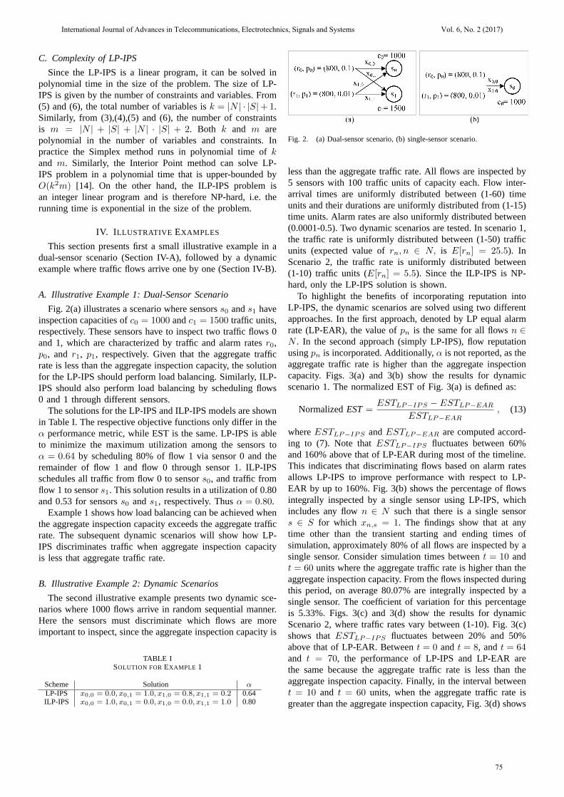
To highlight the benefits of incorporating reputation intoLP-IPS, the dynamic scenarios are solved using two differentapproaches. In the first approach, denoted by LP equal alarmrate (LP-EAR), the value ofpn is the same for all flowsn ∈N . In the second approach (simply LP-IPS), flow reputationusingpn is incorporated. Additionally,α is not reported, as theaggregate traffic rate is higher than the aggregate inspectioncapacity. Figs. 3(a) and 3(b) show the results for dynamicscenario 1. The normalized EST of Fig. 3(a) is defined as:

NormalizedEST =ESTLP−IPS − ESTLP−EAR

ESTLP−EAR

, (13)

whereESTLP−IPS andESTLP−EAR are computed accord-ing to (7). Note thatESTLP−IPS fluctuates between 60%and 160% above that of LP-EAR during most of the timeline.This indicates that discriminating flows based on alarm ratesallows LP-IPS to improve performance with respect to LP-EAR by up to 160%. Fig. 3(b) shows the percentage of flowsintegrally inspected by a single sensor using LP-IPS, whichincludes any flown ∈ N such that there is a single sensors ∈ S for which xn,s = 1. The findings show that at anytime other than the transient starting and ending times ofsimulation, approximately 80% of all flows are inspected by asingle sensor. Consider simulation times betweent = 10 andt = 60 units where the aggregate traffic rate is higher than theaggregate inspection capacity. From the flows inspected duringthis period, on average 80.07% are integrally inspected by asingle sensor. The coefficient of variation for this percentageis 5.33%. Figs. 3(c) and 3(d) show the results for dynamicScenario 2, where traffic rates vary between (1-10). Fig. 3(c)shows thatESTLP−IPS fluctuates between 20% and 50%above that of LP-EAR. Betweent = 0 and t = 8, andt = 64and t = 70, the performance of LP-IPS and LP-EAR arethe same because the aggregate traffic rate is less than theaggregate inspection capacity. Finally, in the interval betweent = 10 and t = 60 units, when the aggregate traffic rate isgreater than the aggregate inspection capacity, Fig. 3(d) shows


75

Fig. 3. (a), (b): Results for the dynamic scenario 1, forrn uniformly distributed between (1-50),n ∈ N . (a) Normalized expected suspicious traffic inspectedby sensors, computed according to Eq. (13), (b) Percentage of flows integrally inspected by a single sensor using LP-IPS, (c), (d): Results for the dynamicScenario 2, forrn uniformly distributed between (1-10).

that an average of 95.5% of inspected flows are integrallyinspected by a single sensor. The coefficient of variation forthis percentage is 0.87%.

The results in Fig. 3(b) and Fig. 3(d) indicate that thepercentage of flows integrally inspected by a single sensor issensitive to the size of the flow rates with respect to the IPSinspection capacities. Larger numbers of flows with smallerflow rates (rn) are inspected by a single sensor,n ∈ N . Thisis confirmed in Section V-B, as presented next.

V. PRESERVATION OFSTATE INFORMATION

This section presents an analysis of how Simplex solves LP-IPS. Section V-A shows that the solutions by Simplex permitthe collection of state information. Section V-B provides anapproximation of the percentage of traffic flows for which stateinformation can be collected.

A. Simplex Solution for LP-IPS

As observed in Figs. 3(b) and 3(d), LP-IPS allows for statepreservation without imposing integral constraints. This is akey result to efficiently solve the scheduling problem. ConsiderFig. 2(b), where two flows are inspected by a single sensor.Assume that the only objective is the maximization of the EST,i.e. w1 = 1, w2 = 0, andα = 1. The corresponding LP, incanonical form, is defined by (14)-(17).

80x0,0 + 8x1,0 = F, (14)

x0,0 + x′

0,0 = 1, (15)

x1,0 + x′

1,0 = 1, (16)

800x0,0 + 800x1,0 + xs0= 1000. (17)

The basic variablesx′

0,0 = 1, x′

1,0 = 1, and xs0 =1000 are shown in bold. The variablesx′

0,0, x′

1,0, and xs0

are slack variables used to drive the problem into canon-ical form. The current basic feasible solution is given by(x0,0;x1,0;x

′

0,0;x′

1,0;xs0) = (0; 0; 1; 1; 1000). The basic vari-ables are also the slack variables, and the objective value isF0. In Eq. (14), the coefficient of the variablex0,0 is positive(80); thus, Simplex will attempt to maximize the variablex0,0,making it a new basic variable in the next iteration. The leavingbasic variable is obtained from Constraints (15) and (17) as:

x′

0,0 = 1− x0,0 ≥ 0, xs0 = 1000− 800x0,0 ≥ 0. (18)

The maximum value that satisfies both constraints is:

x0,0 = min

{

1,1000

800

}

= 1. (19)

The leaving basic variable isx′

0,0, i.e., by settingx0,0=1,Simplex schedules flow 0 integrally. Note that this would stillbe the case in a multi-sensor scenario. The ratio1000

800in Eq.

(19) is the residual capacity of sensors0 to the flow rater0being scheduled. The revised linear program with the objectivefunction expressed in term of non-basic variables is defined byEqs. (20)-(23).

8x1,0 − 80x′

0,0 = −80 + F, (20)

x0,0 + x′

0,0 = 1, (21)

x1,0 + x′

1,0 = 1, (22)

800x1,0 − 800x′

0,0 + xs0= 200. (23)

The current basic feasible solution is given by(x0,0;x1,0;x

′

0,0;x′

1,0;xs0) = (1; 0; 0; 1; 200). The basic


76

variables arex0,0, x′

1,0, andxs0 , and the objective function isF = 80. Note how Simplex integrally schedules flow 0 ratherthan fractional values of flows 0 and 1, permitting sensors0to maintain state information for flow 0. In the next iteration,x1,0 becomes the new basic variable because its coefficient in(20) is positive, and the leaving basic variable is determinedby Constraints (22) and (23):

x′

1,0 = 1− x1,0 ≥ 0, xs0 = 200− 800x1,0 ≥ 0. (24)

The maximum value that satisfies both constraints is:

x1,0 = min

{

1,200

800

}

=1

4. (25)

The leaving basic variable isxs0 , which indicates that sensors0 will not have any residual capacity in the next iteration.Simplex maximizes the entering basic variablex1,0 to 200

800=

1

4, which is the ratio of residual sensor capacity to the flow

rater1. Eqs. (26)–(29) are the last iteration of Simplex.

− 72x′

0,0 −1

100xs0 = −82 + F, (26)

x0,0 + x′

0,0 = 1, (27)

x′

0,0 + x′

1,0 −1

800xs0 =

3

4, (28)

x1,0 − x′

0,0 +1

800xs0 =

1

4. (29)

The coefficients of the non-basic variablesx′

0,0 and xs0

in Eq. (26) are negative. Since the linear program is incanonical form and any feasible solution to the constraintshas non-negative coordinates, the largest possible value forF has been reached (F= 82). This value is assumedat (x0,0;x1,0;x

′

0,0;x′

1,0;xs0) = (1; 1

4; 0; 3

4; 0). The variables

of interest with physical representation arex0,0 = 1 andx1,0 = 1

4, which indicate that 100% and 25% of flows 0 and

1 respectively will be inspected.A key observation from the above is that the new entering

basic variablexe,0 at each iteration,e ∈ N , is the flow to bescheduled by Simplex, and is given by:

xe,0 = min

{

1,cress0

re

}

, (30)

where cress0is the residual capacity of sensors0. During the

initial iteration, flow 0 is scheduled integrally, see (19). Theindicator that flow 0 is integrally scheduled is determined bysetting xe,0 = 1, which is the general case, provided theresidual capacitycress0

is greater than the traffic ratere.

B. State Information Collection: A Simple Approximation

Note that Figs. 3(b) and 3(d) indicate that the number oftraffic flows integrally inspected by a single sensor dependson sensor capacity and expected traffic rate. LetE[rn] be theexpected value of the traffic rate for flown ∈ N and assumethat all sensors have the same inspection capacity, i.e.cs=cfor all s ∈ S. Assume thatc > E[rn], which is the case forenterprise IPS sensors, and define the ratio of sensor capacityto expected traffic as:

Q = round

(

c

E[rn]

)

. (31)

On average one can assume that half of the|S| sensors willinspectQ flows integrally and the other half will inspectQ−1flows integrally. The approximate number of flows integrallyinspected is:

I ≈|S|

2Q+

|S|

2(Q− 1) =

|S|

2(2Q− 1). (32)

Sensors use their residual capacity to inspect fractions offlows, see (30). Thus, after inspecting integral flows, a sensorwould only inspect one fractional flow, i.e. Simplex attempts tofully schedule one flow before scheduling another. On averagethere would be|S| fractional flows, i.e. one flow per sensor.The ratio of the total number of flows integrally inspected bya single sensor to the total number of flows inspected is thenapproximated as:

ratio≈I

I + |S|=

2Q− 1

2Q+ 1. (33)

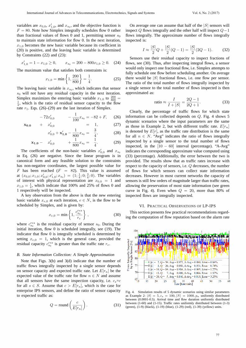
Clearly, the percentage of traffic flows for which stateinformation can be collected depends onQ. Fig. 4 shows 5dynamic scenarios where the input parameters are the sameas those in Example 2, but with different traffic rate.E[rn]is denoted byE[r], as the traffic rate distribution is the samefor all n ∈ N . “Avg” indicates the ratio of flows integrallyinspected by a single sensor to the total number of flowsinspected, in the[10 − 60] interval (percentage). “A-Avg”indicates the corresponding approximate value computed using(33) (percentage). Additionally, the error between the two isprovided. The results show that as traffic rates increase withrespect to the capacity of sensors, i.e.Q decreases, the numberof flows for which sensors can collect state informationdecreases. However in most current networks the capacity ofsensors is still few orders of magnitude larger than traffic rates,allowing the preservation of most state information (see greencurve in Fig. 4). Even whenQ = 20, more than 80% ofinspected flows are integrally inspected.

VI. PRACTICAL OBSERVATIONS OFLP-IPS

This section presents few practical recommendations regard-ing the computation of flow reputation based on the alarm rate

Fig. 4. Simulation results of 5 dynamic scenarios using similar parametersas Example 2:|S| = 5, cs = 100, |N | = 1000, pn uniformly distributedbetween (0.0001-0.5). Arrival time and flow duration uniformly distributedbetween (1-60) and (1-15). Traffic rates uniformly distributed between (1-3)(green), (1-9) (black), (1-19) (blue), (1-29) (red), (1-39) (yellow) units.


77

metric (Section VI-A) and the implementation of IPS jointlywith access-control lists (Section VI-B).

A. Flow Sampling and Reputation

In an ideal scenario all traffic entering a network shouldbe inspected. However, as the amount of traffic increases, animproved discrimination mechanism based on flow reputationis needed. Information about flows (such as source address,destination address, source port, destination port, and trafficrate) can be dynamically obtained from devices such as routersand switches. Many modern routers and switches include flowmanagement applications such as Netflow [15].

The LP-IPS model does not include any requirement toforce at least a minimum sampling of flows to continuouslyupdate the respective alarm rates. Instead this requirement canbe met independently of LP-IPS, or alternatively, it can alsobe incorporated as follows:

∑

s∈S rnxn,s ≥ δn, n ∈ N. Thisconstraint requires sensors to inspect a minimum amount oftraffic δn and to report all alarmsAn raised during inspection.This information can be used to calculate the alarm ratepn. Note thatpn can be considered as a point estimate ofa signature inspectionmatch probability. Assuming thatpnfollows a binomial distribution, a minimum sample sizeδnfor estimating the match probability can be computed givena maximal margin of errorE for a confidence levelL:δn = pn(1−pn)

(

zLE

)2. The parameterzL is the critical value

from the normal distribution for the confidence levelL [16].In order to capture dynamic conditions where intrusion

attempts may occur, it may be desirable to continuously updatethe alarm ratepn. One approach is to use an exponentialaverage of the previous alarm rates. Eq. (1) can include atime dimensionpn(t) = An

rn(t), which measures the alarm

rate during the interval betweent and t + 1. For 0 ≤ λ ≤ 1,the predicted alarm rate att + 1 is given by: p̂n(t + 1) =λpn(t)+(1−λ)p̂n(t). pn(t) stores the most recent information,whereasp̂n(t) tracks past history. The parameterλ controlsthe relative weight of recent and past history. Ifλ = 1, thenp̂n(t + 1) = pn(t), i.e. only the recent alarm rate mattersand history is irrelevant. Note that̂pn(0) can be defined as aconstant. For example, flows inspected for the first time forwhich there are no alarm records would have a largep̂n(0)value. According to the objective function (2), LP-IPS wouldthen maximize the inspected traffic from this flow. Over time,p̂n(t) will be adjusted according to the above exponentialaverage expression.

B. Access Control Lists

Commercial IPS sensors have the capability to block trafficfrom a particular flow, commonly specified in an accesscontrol list (ACL). An ACL is a sequential list of permit ordeny statements that apply to IP addresses and upper-layerprotocol features, such as ports. A black ACL consists offlows that are blocked (from attacking systems) and do notconsume any IPS resources. One advantage of this blockingaction is that a single IPS sensor can stop traffic at multiplelocations throughout the network, regardless of its location.For example, in a multi-homed network that has more than

one connection to external networks, several independent IPSsensors can be deployed. If a set of sensors detects a high levelof matching signatures, that set can add the corresponding flowto a black ACL and apply the ACL to itself and other sensors.A white ACL consists of flows that are completely trusted anddo not require inspection. Both white and black ACLs releasecomputational resources as their listed flows are not inspectedby IPS sensors. Since ACLs are implemented in the forwardinghardware of a device, they do not compromise performance.Such mechanisms are preferred to secure a SDMZ [4].

VII. C ONCLUSION

This paper presents an optimization scheme to maximizethe amount of suspicious traffic inspected by IPS sensors.The scheme uses flow reputation to prioritize the inspectionof flows with high alarm rates. An additional feature ofthe scheme is the load balancing by which traffic flows arescheduled according to the capacity of sensors.

An analysis of how Simplex solves the LP-IPS modeldemonstrates that state information can be preserved withoutimposing integral constraints (i.e., correlating data across mul-tiple packets with specific composite signatures is achievable).Results show that the number flows for which state informationis collected depends on the ratio IPS sensor capacity to trafficflow rates (size). In simulated scenarios, when this ratio is50 (IPS sensor capacity is 50 times that of flow rates), thepercentage of flows for which sensors can correlate data acrossmultiple packets is above 95%. Even when this ratio is only20, the percentage of flows for which sensors can correlatedata across multiple packets is above 80%.

Since LP-IPS is not constrained to integer variables, thescheme can be solved and implemented efficiently. As theabove results indicate, the scheme is effective for protect-ing networks from attacks characterized by both atomic andcomposite signatures. The paper concludes with practicalobservation for the implementation of the proposed scheme.

REFERENCES

[1] V. Sekar, R. Krishnaswamy, A. Gupta, M. Reiter, “Network-WideDeployment of Intrusion Detection and Prevention Systems,”ACMInternational Conference on Emerging Networking Experiments andTechnologies (CoNEXT), Philadelphia, PA, Nov. 2010.

[2] A. Le, E. Al-Shaer, R. Boutaba, “On Optimizing Load Balancingof Intrusion Detection and Prevention Systems,”IEEE InternationalConference on Computer Communications (INFOCOM), Phoenix, AZ,Apr. 2008.

[3] Cisco Systems, [Online]. Available: http://www.cisco.com[4] ESnet, [Online]. Available: http://fasterdata.es.net/science-dmz[5] J. Crichigno, N. Ghani, “A Linear Programming Scheme for IPS Traffic

Scheduling,”IEEE International Conference on Telecommunications andSignal Processing (TSP), Prague, Czech Republic, July 2015.

[6] W. Stallings, “Network Security Essentials,” 5th Edition, Prentice Hall,2013.

[7] H. Jiang, G. Zhang, G. Xie, K. Salamatian, L. Mathy, “Scalable High-Performance Parallel Design for Network Intrusion Detection Systemson Many-Core Processors,”ACM/IEEE Symposium on Architectures forNetworking and Communications Systems, San Jose, CA, Oct. 2013.

[8] L. Foschini, A. Thapliyal, L. Cavallaro, C. Kruegel, G. Vigna, “AParallel Architecture for Stateful, High-Speed Intrusion Detection,”,International Conference on Information Systems Security, Hyderabad,India, Dec. 2008.


78

[9] A. Le, E. Al-Shaer, R. Batouba, “Correlation-Based Load Balancing forIntrusion Detection and Prevention Systems,”International Conferenceon Security and Privacy in Communication Networks, Istanbul, Turkey,Sep. 2008.

[10] L. Zhang, G. Shou, Y. Hu, Z. Guo, “Deployment of Intrusion PreventionSystem Based on Software Defined Networking,”IEEE InternationalConference on Communication Technology (ICCT), Guilin, China, Nov.2013.

[11] S. Laniepce, M. Lacoste, M. Kassi-Lahlou, F. Bignon, K. Lazri, A.Wailly, “Engineering Intrusion Prevention Services for IaaS Clouds:The Way of the Hypervisor,”IEEE International Symposium on ServiceOriented System Engineering (SOSE), San Francisco, CA, Mar. 2013.

[12] T. Xing, D. Huang, L. Xu, C. Chung, P. Khatkar, “SnortFlow: AOpenFlow-Based Intrusion Prevention System in Cloud Environment,”GENI Research and Educational Experiment Workshop (GREE2013),Salt Lake City, UT, Mar. 2013.

[13] J. Crichigno, N. Ghani, J. Khoury, W. Shu, M. Wu, “Dynamic Rout-ing Optimization in WDM Networks,”IEEE Global CommunicationsConference (GLOBECOM), Miami, FL, Dec. 2010.

[14] S. Boyd, L. Vandenberghe, “Convex Optimization,”Cambridge Univer-sity Press, 2004.

[15] Netflow, [Online]. Available: http://www.cisco.com/c/en/us/products/ios-nx-os-software/ios-netflow

[16] C. Brase, C. Brase, “Understanding Basic Statistics,” 6th Edition,Cengage Learning, 2012.


79

Documents

Optimal Trafﬁc Scheduling for Intrusion Prevention Systems