Embed Size (px)
Citation preview
1ANALISIS TRIWULANAN: Perkembangan Moneter, Perbankan dan Sistem Pembayaran, Triwulan II - 2007
BULLETIN OF MONETARY ECONOMICS AND BANKING
Directorate of Economic Research and Monetary PolicyBank Indonesia
PatronPatronPatronPatronPatronBoard of Governor Bank Indonesia
Editorial BoardEditorial BoardEditorial BoardEditorial BoardEditorial BoardProf. Dr. Anwar Nasution
Prof. Dr. Miranda S. GoeltomProf. Dr. Insukindro
Prof. Dr. Iwan Jaya AzisProf. Iftekhar HasanDr. M. Syamsuddin
Dr. Perry WarjiyoProf. Masaaki Komatsu
Dr. Iskandar SimorangkirDr. Solikin M. JuhroDr. Haris Munandar
Dr. Andi M. Alfian Parewangi
Editorial ChairmanEditorial ChairmanEditorial ChairmanEditorial ChairmanEditorial ChairmanDr. Perry Warjiyo
Dr. Iskandar Simorangkir
Executive DirectorExecutive DirectorExecutive DirectorExecutive DirectorExecutive DirectorDr. Andi M. Alfian Parewangi
SecretariatSecretariatSecretariatSecretariatSecretariatArifin M. Suriahaminata, MBA
MS. Artiningsih, MBA
The Bulletin of Monetary Economics and Banking (BEMP) is a quarterly accredited journalpublished by Directorate of Economic Research and Monetary Policy Bank Indonesia. Theviews expressed in this publication are those of the author(s) and do not necessarily reflectthose of Bank Indonesia.
We invite academician and practitioners to write on this journal. Please submit your paper andsend it via mail to: [email protected]. See the writing guidance on the back of thisbook.
This journal is published on; January √ April √ August √ October. The digital version includingall back issues are available online; please visit our link: √http://www.bi.go.id/web/id/Publikasi/Jurnal+Ekonomi/. If you are interested to subscribe for printed version, please contact ourdistribution department: Publication and Administration Section √ Directorate of Economyand Monetary Statistics, Bank Indonesia, Building Sjafruddin Prawiranegara, 2nd Floor - Jl. M.H. Thamrin No.2 Central Jakarta, Indonesia, Ph. +62-21-3818202, Fax. +62-21-3802283,Email: [email protected].

BULLETIN OF MONETARY ECONOMICSAND BANKING
Volume 14, Number 3, January 2012
QUARTERLY ANALYSIS: The Progress of Monetary, Banking and Payment System,
Quarter IV - 2011
Author Team of Quarterly Report, Bank Indonesia
Market Power of Indonesian Banking
Andi Fahmi Lubis
The Impact of Excess Liquidity on Monetary Policy
M. Barik Bathaluddin, Nur M. Adhi P., Wahyu A.W.
Transmission Channel and Effectiveness of Dual Monetary Policy In Indonesia
Ascarya
Analysis of Sectoral Efficiency and the Response of Regional Policy
M. Abdul Majid Ikram, Andry Prasmuko, Donni Fajar Anugerah, Ina Nurmalia Kurniati
225
269
221
245
299

1ANALISIS TRIWULANAN: Perkembangan Moneter, Perbankan dan Sistem Pembayaran, Triwulan II - 2007
221QUARTERLY ANALYSIS: The Progress of Monetary, Banking and Payment System, Quarter IV, 2011
QUARTERLY ANALYSIS:The Progress of Monetary, Banking and Payment System
Quarter IV √ 2011
Author Team of Quarterly Report, Bank Indonesia
The Board of Governor Meeting of Bank Indonesia today decided to maintain the BI rateat the level of 6.0%. This decision is based on thoroughly examination on the recent economic
performance, several recent risks, and the prospect of the economy. The Board of Governor
view the level of BI rate is consistent with the targeted inflation ahead, and is conducive tomaintain the financial stability, and also to mitigate the impact of global prospect on Indonesian
economy.
In general, the evaluation of the performance and the prospect of Indonesian economyshow the domestic economy remain strong and stable. Looking ahead, the Board of Governor
will keep examining the risk of global economic worsening, maintain the macroeconomic and
financial system stability, and stimulate the domestic economy. Board of Governor emphasizethe mix of monetary and the other micro prudential policies, which is counter cyclical, is necessary
on macroeconomic management and drive the actual inflation to the target of 4,5%±1% in
2012 and 2013.
Board of Governor noted the economy in 2011 was slowing down, mainly due to the
uncertainty of economic and financial recovery in Europe and United States. The crisis escalation
in Europe particularly on second semester 2011 triggered a high volatility in global financialmarket. With the reduction of global demand, the global trade volume and commodity price
also decreased.
On price side, the inflation pressure in developed countries increased, while in emerging
countries is moderate though still in high level. Along with this progress, by the end of 2011,the emerging market tended to choose neutral or slightly accommodative, while the developing
countries maintained the accommodative monetary policy with liquidity easing.
On domestic side, the Board of Governor considered the economic performance in 2011was still strong. This achievement is supported by the maintained macro and financial system
stability. The economic growth in quarter IV 2011 is expected to be 6.5%; hence the economic
growth in 2011 will be 6.5% (yoy). This growth is mainly triggered by the strong domesticdemand and the maintained export performance. From production side, the main pro-growth
sectors are Manufacture, Transport and Telecommunication and Hotel, Trade and Restaurant.

222 Bulletin of Monetary Economics and Banking, January 2012
The performance of Indonesian Balance of Payment (BOP) for the whole 2011 recorded
large surplus, even though there was a pressure on semester II, 2011. The pressure was on thecapital and financial transaction, along with the increase of global economic and financial
market uncertainty.
Several policies of Bank Indonesia and government have helped to restrain the pressureon Rupiah exchange rate. During 2011, the trend is till consistent with the regional exchange
rate movement. Bank Indonesia keep monitoring the dynamics of Rupiah and its stability and
make sure it moves along with its fundamental.
On price side, the inflation decrease in 2011. CPI inflation on November 2011 was recorded0.034% (mtm) or 4.15% (yoy). The decline of inflation during 2011 occurred due to correction
on volatile food prices inflation and minimum administered price inflation, while the core inflation
tended to be moderate. The low of volatile food price inflation was supported by the wellmaintained supplies, either from domestic or import. Even though the rice recorded quite high
inflation, there were major price corrections on seasoning such as onion, red chili and on the
meat.
Meanwhile, the well-controlled inflation was supported by the sharp declining of the
global commodity prices, the stability of exchange rate and a better inflation expectation. If the
decline inflation continues, the overall CPI inflation for 2011 is expected to be lower than4.0%.
The stability of banking system is well maintained with better intermediation function,
even there was fluctuation on financial market because of the global influence. Banking industryis solid as reflected on high capital sufficiency (CAR, Capital Adequacy Ratio); way above the
required minimum level of 8%, and also reflected on the maintained gross Non-Performing
Loan (NPL) of below 5%. Meanwhile, the loan growth until the end of October 2011 reached25.7% (yoy), consisting of investment loan by 31.1% (yoy), working capital loan 24.7% (yoy),
and consumption loan 23.8% (yoy). With these progresses, the growth of loan for the whole
2011 will accord the Bank Business Plan.
The reliability and efficiency of payment system support the stability of financial system.As supporting infrastructure for economic activities, the payment system ensures the payment
transaction of all economic agents. The supports of the payment system on the economic
performances are reflected by several Bank Indonesia policies, including the standardized chipbased ATM/debit card, the improvement of card payment system, the development of Bank
Indonesia Real Time Gross Settlement (BI-RTGS), the second generation of Bank Indonesia
Scrip less Security Settlement System (BI-SSSS), the development of National Payment Gateway-NPG, the increase of government account management, and the preparation of standardized
electronic money.
223QUARTERLY ANALYSIS: The Progress of Monetary, Banking and Payment System, Quarter IV, 2011
Looking ahead, the global economic growth is expected to slow down due to the high
uncertainty of debt and fiscal settlement in Europe and US. This global slowing down willaffect the domestic economy growth in 2012 to be around 6.3% - 6.7%. For 2013, the
growth is expected to be in the range of 6.4% - 6.8%, along with the global economic
improvement. On price side, the Board of Governor predicts the inflation in 2012 and 2013can be directed to the target of 4.5% + 1%.
Related to this, the reduction of BI rate, which has been done so far, is expected to
stimulate the economy. The Board of Governor is aware of several risks impact on themacroeconomic balances, including the worsening of global economy. Along with this, beside
continuing the monetary and financial system stabilization by ensuring the sufficiency of Rupiah
liquidity and foreign exchange on the market, Bank Indonesia will keep optimize the momentumof interest rate decline to optimize the effectiveness of stimulus on the economy. In addition,
Bank Indonesia continues and strengthens to coordinate with the government in order to
increase the stimulus from fiscal and the real sector.

224 Bulletin of Monetary Economics and Banking, January 2012
This page is intentionally left blank
225Market Power of Indonesian Banking
MARKET POWER OFINDONESIAN BANKING
Andi Fahmi Lubis 1
This study aimed to estimate the degree of market power exercised by commercial banks in the
credit market in Indonesia. The model used to answer this study»s objective was the Bresnahan-Lau oligopoly
model that uses structural equations to estimate the degree of market power. This model uses a very
different approach than Structure-Conduct-Performance (SCP) paradigm commonly used in market power
studies. Without using actual cost data and accounting profit, the Bresnahan-Lau model was able to
estimate directly the degree of market power from the structural equations. The main result of this study
showed that the degree of market power exercised by commercial banks in the credit market is relatively
low; in other words, the degree of competition in the credit market in Indonesia is quite high.
1 The author is a lecturer at Master of Planning and Public Policy of Economic and Business Faculty, University of Indonesia;[email protected]. Points of view and conclusions in this paper are solely of the author and do not necessarily represent any otherinstitution. The author is deeply thankful to the anonymous referee for the comment and suggestions on this paper.
Abstract
Keywords: market power, oligopoly, Bresnahan-Lau, structure, performance, conduct, SCP.
JEL Classification : L13, G21

226 Bulletin of Monetary Economics and Banking, January 2012
I. INTRODUCTION
Market power is a measure of performance that shows how much a firm can increase
the price above the marginal cost (Church and Ware, 2000). Associated with the market structure,
a firm in perfectly competitive market does not have any market power, while a firm in amonopoly market has the strongest market power. Thus it can be concluded that the more
competitive a market is, the lower the market power of a firm; conversely, the more uncompetitive
a market is, the higher the market power of a firm.
Analysis of the level of competition in a market using market power measurementhas been a major focus in industrial economic studies, including assessments of the level of
competition in the banking industry. As an industry that serves as intermediary institutions
between those who have excess funds (surplus spending units) and those who need thefunds, the banks play a very vital role in supporting the process of development. If distortion
occurs in the banking industry, which generates an inefficient performance, then the
intermediary process between those who need funds and fund owners will have somebarriers. The existence of these barriers would hinder the funds to finance projects for
development.
Considering the importance of the banking function for the development of economy,the government will try to keep the banking industry performing its intermediaries function.
Various government policies will be taken to increase efficiency in the banking industry.
Indonesia»s banking industry had experienced significant developments since the implementationof the deregulation package in 1983, which Cole and Slade (1996) called the phase of
Reformation in 1983, followed by the phase of free-entry in 1988, famously known as PAKTO
88. The impact of the deregulation was the increase of banking intermediaries function reflectedby the increase of the collected third party funds and the distributed loan. The deregulation
was surely believed to increase the efficiency of banking industry reflected by the decrease of
concentration level in banking industry.
The decrease of concentration level in a market will give a positive impact on market
efficiency according to Structure-Conduct-Performance (SCP) approach, in which the
performance of a market depends on its structure. The more concentrated a market, the greaterthe ability of a firm to increase the price above the marginal cost, reflecting a higher market
power. This higher market power indicates lower competition level.
The competition level based on the concentration ratio is the main hypothesis construction
for the studies using SCP approaches. The concentration level of Indonesian banking industrydeclined after deregulation in 1983 and 1988, but after this period it tended to be stable at
concentrations level of CR4 by 40-50»s and CR8 by»50-60»s. Table 1 shows that the concentration
level of banking industry in Indonesia is still at the middle level, and has not reached competitivelevels.

227Market Power of Indonesian Banking
Analysis of market power based on the SCP approach that uses structure as an indication
of the competition level in the market raises many criticisms. Among them is the endogeneityproblem between the structure and the performance, where the SCP approach assumes the
existence of a one-directional relationship between structure and performance; thereby asserting
market performance can be indicated from the existing market structure. Another criticism isassociated with the use of accounting profit or price cost margin (PCM) as a proxy of the
difference between price and marginal cost. The weakness of SCP approach raised a new
approach that tries to analyze the level of competition in the market that was not based on thestructure of the market, but based on the behavior of existing firms in the market. New Industrial
Economics (NIE) approach estimates the size of market power in a market, which is then used
as an indicator of the competition level. One of the estimation models in this new approach isthe oligopoly model developed by Bresnahan (1982) and Lau (1982).
Table 1.Bank’s Rating during the Loan Period of 2000 and 2005
Year2000
12345678
* = until March 2005
Source: SEKI of Bank Indonesia
Bank’s NameLoanShare
(%)
Year2005 Bank’s Name
LoanShare
(%)
Bank MandiriBank Negara IndonesiaBank Rakyat IndonesiaBan Int’l IndonesiaCitibank N. A.HSBCBank Tabungan NegaraBank Central Asia
14.9510.989.426.614.472.912.712.68
12345678
Bank MandiriBank Rakyat IndonesiaBank Negara IndonesiaBank Central AsiaBank DanamonBank NiagaBank PermataBank Int’l Indonesia
15.8310.8410.087.135.203.842.772.47
CR4 41.96 CR4 43.88CR8 54.73 CR8 58.16
The main goal of this paper is to investigate the limit of Indonesian banking in setting the
price. The power of firms to influence the price in a market shows the strength of their exercisingmarket power and the existing competition level in the market. Considering the market structure
is concentrated on few banks, we predict the competition level within Indonesian banking
industry is relatively low, which also indicates a high market power. Joint hypothesis oncompetition and market power of the loan market in Indonesian banking industry will be
measured and tested using Bresnahan-Lau (BL) oligopoly model framework.
The second part of this paper examines the theory and the derivation of the empirical
model to estimate. The third part will discuss the methodology, while the fourth part will discuss
228 Bulletin of Monetary Economics and Banking, January 2012
the estimation result and its analysis. The conclusion and policy implication will be presented in
the last part of the paper.
II. THEORY
Measurement of market power or the level of competition of an industry can be dividedinto two main approaches. The first is the traditional SCP approach, based on the use of
accounting data relating to the profit and cost to measure the market power. The second
approach emerging lately is the New Industrial Economics (NIE) or the New Empirical IndustrialOrganization (NEIO) that reduces or even eliminates the use of accounting data to measure
market power. NIE approach uses a structural framework for the relationship of demand and
supply to estimate market power. The approach is based on the premise that a firm in perfectlycompetitive market, which is the price takers, and a firm in an imperfect market, which has
market power, will have different reactions on exogenous changes in demand and supply (Church
and Ware, 2000).
As a reconciled mainstream (between traditional SCP mainstream and Chicago), the NewIndustrial Economics did not achieve its popularity by attacking the other, therefore we cannot
easily determine a clear boundary line to distinguish it from previous mainstream. However, wecan at least determine the specific characteristics that put it as «new» mainstream (Lubis, 1997).
There are several characteristic. The first includes the game theory as its tool of analysis.
The most obvious difference between «traditional» and «new» industrial economies is the explicit
presentation of the game theory on the problem being examined. On traditional industrialeconomy, the causality flow was started from the structure to behavior, then to performance.
For example, a profit over «normal» (performance) in industry will be associated with collusive
behavior that occurs due to the high concentration (structure), which is possible with the existenceof barriers to entry.
With the inclusion of the game theory into the industrial economy, the flow of causality-
effect was not only one direction, but it can even flow to all directions. The correlation is notonly from the structure to behavior then performance, but to the set of all possible permutations
of the structure, behavior, and performance (Norman and La Manna, 1992). In the new industrial
economy, the number of firms operating in the market (structure) is determined endogenously,and depends on the type of game chosen by the firm, in terms of the variable options (price,
output, etc.), the timing of decision , number of games played, etc.. All factors within in the
structure, behavior and performance became elements that were determined simultaneously,and were influenced by fundamental factors such as technology (or technological opportunities),
demand conditions, and the degree of symmetrical acquired information. Factors such as the
barriers to entry or firm-specific advantage now become the decision variables that aredetermined endogenously by the strategic decisions of firms.
229Market Power of Indonesian Banking
The second important characteristic of the NIE is its higher concern on the role of behavior
(conduct) in the form of appreciation for the strategic dimension of corporate decisions. Thefirm does not react and adapt only towards external conditions, but also tries to make the
economic environment where he belongs, give some advantages to him, considering his
competitors will also do the same (Norman and La Manna, 1992).
In any policy formulation, a firm engaged in imperfectly competitive market (particularly
oligopoly) should consider the impact of his policy implementation to its competitors. The
change of price or output determined by a firm does not only affect sales and profits, but canalso affect its competitors» sales and profit, vice versa. Every oligopolist realizes this. Depending
on the completeness and the speed of information obtained, any policy changes of a firm will
quickly be responded and anticipated by other firms.
From the above discussion we conclude there is interdependent characteristic amongfirms operating in an oligopoly market. The existence of this interdependent characteristic
makes oligopolist stay in a situation where optimal decision depends on decisions taken by the
other firms. Thus, in taking the best decision, a firm must be able to make the best guesspossibility on the reaction of its competitors, or alternatively, its decisions should be at least
difficult to be predicted by his competitors (Layard and Walters, 1978).
The use of oligopoly is the strong characteristic of NIE. Although the oligopoly theorywas generally derived from the theories within the Chicago mainstream, it was the NIE approach
that started to use it in empirical studies. Since NIE «fixed» the empirical study of previous
mainstreams, then the NIEW is often referred as the New Empirical Industrial Organization(NEIO).
The weaknesses of the traditional SCP approach in the empirical analysis raised a new
approach that tried to decrease the use of accounting data. Market power level that belongs toa firm was obtained from the estimation to structural models that described the relationship
between demand and supply curves2. Timothy F. Bresnahan (1982) and Lawrence J. Lau (1982)
were the first economists who put forward this approach based on the oligopoly modelframework.
Model used to estimate market power in Indonesia»s banking industry is BL oligopoly
model using structural equation consisting of demand function and price function or supply
(supply relation). Given profit function that belongs to a firm:
(1)
2 Beside using structural model of supply and demand, market power estimation can be also conducted by using static comparisonmethod, which is called as reduced-form approach. Panzar and Rose (1987) used derived revenue function of the firm (firm»sreduced-form revenue function) to indicate firm»s behavior.

230 Bulletin of Monetary Economics and Banking, January 2012
where q is output, P is price, C is variable cost, W is exogenous variables that affects the
marginal cost or supply, and F is fixed costs.
While the market demand function faced by the firm is:
(2)
(3)
(5)
(6)
where Z is exogenous variable that affects demand. By including the demand function (2) into
the profit function (1), then it will be:
By looking for the first derivation of profit function (3) to the change of q, then function
will be:
(4)
Then by assuming the condition is the average of all firms, then:
and, if then equation (5) can be rewritten as:
where the first derivation of the demand function f‘(Q,Z) denotes marginal revenue and the
first derivation of cost function C’(q,W) is the marginal cost. Recall equation λ:
where the shows conjectural variation of the firm. Conjectural variation can
be defined as a change in the overall output of other firms (the rest) that are anticipated by one
firm as the result of changes in the firm»s output (Bikker, 2003).

231Market Power of Indonesian Banking
Referring to the equation (6) we can draw conclusions related to the firm»s ability to play
at market prices.1. For firms that are in a perfectly competitive market, because they are price takers, then
change in a firm»s output would not affect the overall output. It shows that λ = 0, so that
equation (6) will be:
Ωor P = MC
2. If firms form perfect collusion in the market then the increase in output of a firm would befollowed by the increase in firm»s output,
so we got λ = 1
3. If firms compete in Cournot framework, changes in the overall output would be only fromone firm»s output change, without any»retaliation from the rest of the firms.
Ω so that
Thus between perfect competition and perfect collusion, the value of λ will range from
0 to 1, which means it can be used as an indicator to show the market power level or the
competition level that exists in the market. The empirical study of market power estimation tofigure out the competition rate in the market can be conducted by estimating the variable λ.
Therefore, to answer the purpose of the research, this study will estimate the market power of
the Indonesian banking industry by estimating the value of λ obtained from the Bresnahan-Lau (BL) oligopoly model.
As mentioned above, the BL oligopoly model is a structural model consisting of demand
and supply function. The BL oligopoly model formulation was conducted by customizing theprevious demand function (2) and the price function (6). By using the inverse of demand
function (2):
(7)
and with a little adjustment in the price function (6) which is a supply curve function, thenwe get:

232 Bulletin of Monetary Economics and Banking, January 2012
(9)
(10)
3 The verification for this identification problem was conducted by Lau (1982) which he called it as impossibility theorem.4 It is necessary to estimate λ because in the equation (8), variable λ is related to variable Q, while variable q consists of two, q that is
bound with α and q that is bound with β. By this rotation, then q can be separated from which is only bound with α and λ.
Both functions (7) and (8) above can be solved by using a two-stage least squares (2SLS) with
the price P and the output q as a endogenous variable. The value of λ that was obtained from
the estimation of the above structural model can be used to show the strength of marketpower or the competition level in the market.
The demand function specification required to estimate the market power is found by
determining the exogenous variables (Z), which does not only shift the parallel demand curve,
but can also change the slope degree of demand curve (Bresnahan, 1982)3. It can be conductedby inserting an instrumental variable which is the multiplication (cross-term) of price P with
exogenous variable Z, as follow:
(8)
Thus the exogenous variable Z does not only shift the demand curve but also rotates4 it. The
price equation used is:
By using Figure 1, the logic of this structural model can be described as follow. With the
change of exogenous variable Z, the slope degree of the demand curve and intercept willchange. If the market behaves competitively, the rotation of the demand curve around the
previous equilibrium will not change the equilibrium, so it is fixed in (Q1, P
1). However, if the
firm has the market power, there will be a change in the equilibrium to be (Q2, P
2). Thus, the
rotation of the demand curve caused by the exogenous variable Z, gives a different response
between competitive markets and monopoly markets.

233Market Power of Indonesian Banking
Picture 1. Response differencebetween competitive and monopoly markets
Q
D(Z2)
Q2
P1P2
MCC
MCM
D(Z1)MR(Z2)MR(Z1)
Q1
III. METHODOLOGY
Market power in this study uses a quantitative approach by conducting inferential testingto the empirical model that was developed. Basic modeling refers to a variety of empirical
studies that apply the BL oligopoly model, such as Alexander (1988), Steen and Salvanes (1999),
Toolsema (2002), Bikker and Haaf (2002), and Bikker (2003); the last three studies applied theBL oligopoly model in banking industry. Departing from these three models used to estimate
market power in loan market, are two structural equations, the loan demand function and
supply function (cost function).
Referring to the demand function format (9), then the loan demand function used is:
(11)
where CREDIT is the total loans distributed by commercial banks to the private sectors (claimson private sector). For price, we use the interest rates of the working capital loan (SKMK)5,
whereas exogenous variables that affect the loan use Real GDP (GDP) with base year 1993, asan indicator of the public income, 3-months Certificates of Bank Indonesia (SBI3), the number
of branch offices (BRANCH), the inflation rate (INFLATION) and the quantity of loan in the
previous period (CREDIT-1).
5 Besides the interest rate of working capital loan, the interest rate of investment loan can be used, however, because the movementof the both variables run in the same direction, there is almost no difference between using the interest rate of working capital loanor investment loan.

234 Bulletin of Monetary Economics and Banking, January 2012
There are two interaction variables; the interaction between loan interest rate (SKMK)
with GDP and the interaction between SKMK and SB136. These two variables are used torotate the demand curve.
From the supply side, based on equation (10), then demand or cost function of loan can
be specified by the following equation:
where the exogenous variables used as cost determinant indicators of banking loan distribution
is a deposit rate for 1 month-term (SD1), and the inflation rate (INFLATION).
Both of the structural equations in loan markets above were estimated by using TwoStage Least Square method (2SLS). The object of the study is the loan market of commercial
banks (aggregate). Period used in the estimation model is the first quarter of 1990 (Q1: 1990)
until the fourth quarter of 2004 (Q4: 2004). After adjustment, a total of 59 observations wereobtained.
It should be underlined that there was an important test to be conducted on both structural
models, which is the separability test. Technically, this procedure tested whether the interactionof variables used in the model is valid or not.
There are two structural equations in the empirical model, which respectively have one
interaction variable. To estimate the market power λ, then the necessary condition is that bothdemand functions of the credit market are non-separable, which means it is the expected null
hypothesis would be rejected, so that the two
interaction variables, denoted as SKMK * SBI3 and SKMK * GDP, are still valid to use in themodel.
IV. RESULTS AND ANALYSIS
Loan demand model estimation results (11) using Two Stage Least Square (2SLS), ispresented in Table 2. As previously stated, this market power estimation needs both equations
to be non-separable. The result of the separability test conducted with Coefficient Test LR-
Redundant Test is given as follows:
(12)
6 Interaction with other exogenous variables, for instance branch offices and inflation did not give any significant result, so that theyare not included in the model.

235Market Power of Indonesian Banking
Interest rate of market power
F-statistic 4. 073789 Probability 0.022959
Redundant Variables: SKMK*SBI3 SKMK*PDB
Based on the above test, the null hypothesis is rejected at the 5% level of confidence. It can beconcluded that loan demand function is non-separable at interest rates of 3-months Certificates
of Bank Indonesia (SBI3) and income (GDP).
Table 2:Loan Demand Estimation Model
Sources: author»s calculationsNote: The dependent variable is the total loan value. Model Correction was conducted with White Heteroscedasticity
Variable
ConstantaInterest Rate of working capital loan (SKMK)Real GDP (GDP)3-months certificate of Bank IndonesiaLoan (-1)SKMK*SBI3SKMK*PDBBranch OfficesInflation
Adjusted R2DW StatF StatProb (F Stat)
-1. 26E+155. 67E+13
11. 93591. 34E+13
1. 1494-5. 44E+11
-0. 5439-2. 04E+128. 94E+14
0. 93442. 0124
105. 8730. 0000
-2. 02042. 04442. 00052. 13067. 0338
-2. 3886-2. 0687-1. 74962. 9979
Coefficient T-stat
For t-statistics test with null hypothesis H0: β = 0, it indicates that the value of t-statistics
of all independent variables rejected the null hypothesis at the 5% level of confidence. In other
words, all independent variables, the interest rate of working capital loan (SKMK), Real GDP(GDP), 3-months Certificates of Bank Indonesia (SBI), branch offices (BRANCH), inflation rate
(INFLATION) and Credit lag variable(-1), and the interaction variable (cross-term) between SKMK
with GDP (SKMK * GDP) and SKMK with SBI3 (SKMK * SBI3), significantly (statistically significant)have a relationship with the dependent variable which is credit demand.
The influence of the interest rate of the working capital loan (SKMK) to the total loan
value demand works in two ways; direct and indirect effects. The direct effect is shown by the
236 Bulletin of Monetary Economics and Banking, January 2012
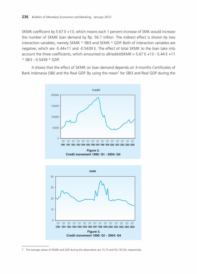
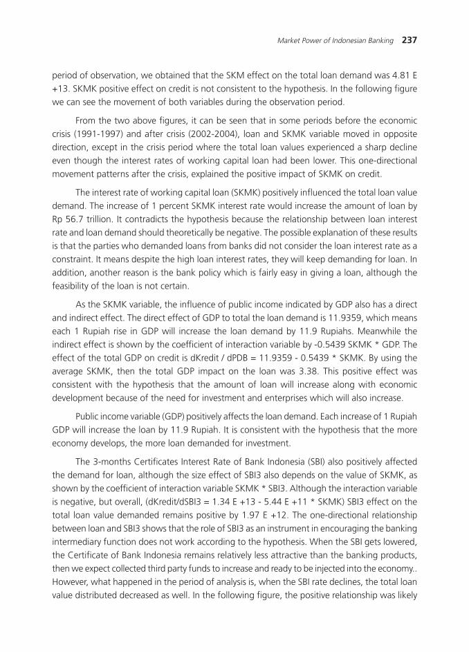
Figure 2.Credit movement 1990: Q1 - 2004: Q4
Figure 3.Credit movement 1990: Q1 - 2004: Q4
Credit
0
50000
100000
150000
200000
1990 1991 1992 1993 1994 1995 1996 1997 1998 1999 2000 2001 2002 2003 2004Q1 Q1 Q1 Q1 Q1 Q1 Q1 Q1 Q1 Q1 Q1 Q1 Q1 Q1 Q1
SKMK
1990 1991 1992 1993 1994 1995 1996 1997 1998 1999 2000 2001 2002 2003 2004Q1 Q1 Q1 Q1 Q1 Q1 Q1 Q1 Q1 Q1 Q1 Q1 Q1 Q1 Q1
0
10
20
30
40
SKMK coefficient by 5.67 E +13, which means each 1 percent increase of SMK would increase
the number of SKMK loan demand by Rp. 56.7 trillion. The indirect effect is shown by twointeraction variables, namely SKMK * SBI3 and SKMK * GDP. Both of interaction variables are
negative, which are -5.44+11 and -0.5439 E. The effect of total SKMK to the loan take into
account the three coefficients, which amounted to dKredit/dSKMK = 5.67 E +13 - 5.44 E +11* SBI3 - 0.5439 * GDP.
It shows that the effect of SKMK on loan demand depends on 3-months Certificates of
Bank Indonesia (SBI) and the Real GDP. By using the mean7 for SBI3 and Real GDP during the
7 The average values of SKMK and GDP during the observation are 15.73 and 92,135.04, respectively.
237Market Power of Indonesian Banking
period of observation, we obtained that the SKM effect on the total loan demand was 4.81 E
+13. SKMK positive effect on credit is not consistent to the hypothesis. In the following figurewe can see the movement of both variables during the observation period.
From the two above figures, it can be seen that in some periods before the economic
crisis (1991-1997) and after crisis (2002-2004), loan and SKMK variable moved in oppositedirection, except in the crisis period where the total loan values experienced a sharp decline
even though the interest rates of working capital loan had been lower. This one-directional
movement patterns after the crisis, explained the positive impact of SKMK on credit.
The interest rate of working capital loan (SKMK) positively influenced the total loan valuedemand. The increase of 1 percent SKMK interest rate would increase the amount of loan by
Rp 56.7 trillion. It contradicts the hypothesis because the relationship between loan interest
rate and loan demand should theoretically be negative. The possible explanation of these resultsis that the parties who demanded loans from banks did not consider the loan interest rate as a
constraint. It means despite the high loan interest rates, they will keep demanding for loan. In
addition, another reason is the bank policy which is fairly easy in giving a loan, although thefeasibility of the loan is not certain.
As the SKMK variable, the influence of public income indicated by GDP also has a direct
and indirect effect. The direct effect of GDP to total the loan demand is 11.9359, which meanseach 1 Rupiah rise in GDP will increase the loan demand by 11.9 Rupiahs. Meanwhile the
indirect effect is shown by the coefficient of interaction variable by -0.5439 SKMK * GDP. The
effect of the total GDP on credit is dKredit / dPDB = 11.9359 - 0.5439 * SKMK. By using theaverage SKMK, then the total GDP impact on the loan was 3.38. This positive effect was
consistent with the hypothesis that the amount of loan will increase along with economic
development because of the need for investment and enterprises which will also increase.
Public income variable (GDP) positively affects the loan demand. Each increase of 1 Rupiah
GDP will increase the loan by 11.9 Rupiah. It is consistent with the hypothesis that the more
economy develops, the more loan demanded for investment.
The 3-months Certificates Interest Rate of Bank Indonesia (SBI) also positively affectedthe demand for loan, although the size effect of SBI3 also depends on the value of SKMK, as
shown by the coefficient of interaction variable SKMK * SBI3. Although the interaction variable
is negative, but overall, (dKredit/dSBI3 = 1.34 E +13 - 5.44 E +11 * SKMK) SBI3 effect on thetotal loan value demanded remains positive by 1.97 E +12. The one-directional relationship
between loan and SBI3 shows that the role of SBI3 as an instrument in encouraging the banking
intermediary function does not work according to the hypothesis. When the SBI gets lowered,the Certificate of Bank Indonesia remains relatively less attractive than the banking products,
then we expect collected third party funds to increase and ready to be injected into the economy..
However, what happened in the period of analysis is, when the SBI rate declines, the total loanvalue distributed decreased as well. In the following figure, the positive relationship was likely
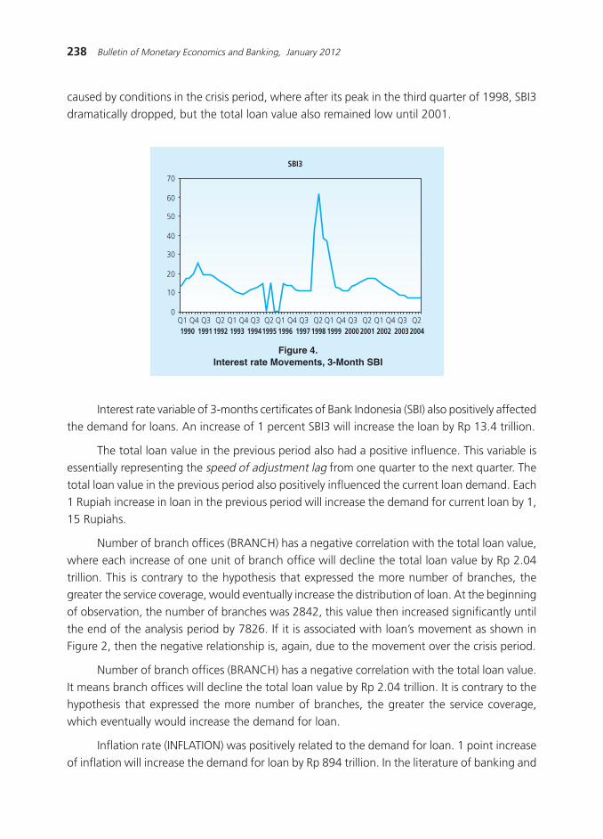
238 Bulletin of Monetary Economics and Banking, January 2012
caused by conditions in the crisis period, where after its peak in the third quarter of 1998, SBI3
dramatically dropped, but the total loan value also remained low until 2001.
Figure 4.Interest rate Movements, 3-Month SBI
SBI3
0
10
20
30
40
50
60
70
1990Q1 Q4 Q3
1991Q2
1992 1993Q1 Q4 Q3
1994Q2
1995 1996Q1 Q4 Q3
1997Q2
1998 1999Q1 Q4 Q3
2000Q2
2001 2002Q1 Q4 Q3
2003Q2
2004
Interest rate variable of 3-months certificates of Bank Indonesia (SBI) also positively affected
the demand for loans. An increase of 1 percent SBI3 will increase the loan by Rp 13.4 trillion.
The total loan value in the previous period also had a positive influence. This variable isessentially representing the speed of adjustment lag from one quarter to the next quarter. The
total loan value in the previous period also positively influenced the current loan demand. Each
1 Rupiah increase in loan in the previous period will increase the demand for current loan by 1,15 Rupiahs.
Number of branch offices (BRANCH) has a negative correlation with the total loan value,
where each increase of one unit of branch office will decline the total loan value by Rp 2.04
trillion. This is contrary to the hypothesis that expressed the more number of branches, thegreater the service coverage, would eventually increase the distribution of loan. At the beginning
of observation, the number of branches was 2842, this value then increased significantly until
the end of the analysis period by 7826. If it is associated with loan»s movement as shown inFigure 2, then the negative relationship is, again, due to the movement over the crisis period.
Number of branch offices (BRANCH) has a negative correlation with the total loan value.
It means branch offices will decline the total loan value by Rp 2.04 trillion. It is contrary to thehypothesis that expressed the more number of branches, the greater the service coverage,
which eventually would increase the demand for loan.
Inflation rate (INFLATION) was positively related to the demand for loan. 1 point increase
of inflation will increase the demand for loan by Rp 894 trillion. In the literature of banking and
239Market Power of Indonesian Banking
loan, the relationship between inflation and loan demand can be uni-direction or bi directional8.
Explanation on this positive relationship is a firm using two funding resources to finance workingcapital, i.e. money (own capital) and capital loans (from banks). The high inflation rate penalizes
the firm for using much more of its own capital; hence the loan from bank would be more
desirable.
Inflation rate (INFLATION) was positively related to demand for loan. The increase of 1
point will increase the demand for a loan by Rp 894 trillion. Meanwhile, both interaction variables
significantly influenced the demand for credit, but this will not be specifically analyzed becauseits function is to determine the market power level acquired by Bank Indonesia.
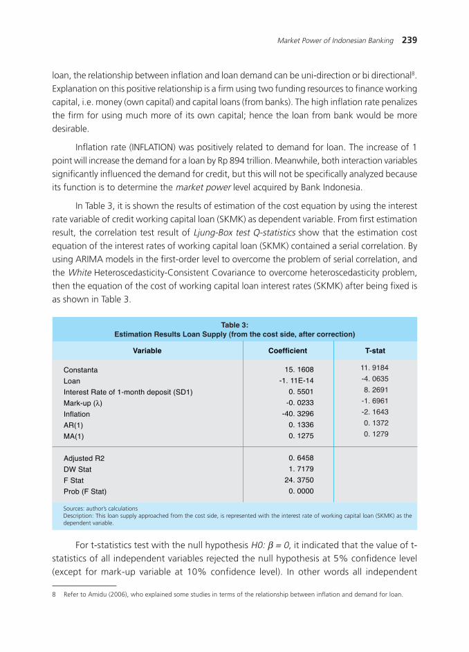
In Table 3, it is shown the results of estimation of the cost equation by using the interest
rate variable of credit working capital loan (SKMK) as dependent variable. From first estimation
result, the correlation test result of Ljung-Box test Q-statistics show that the estimation costequation of the interest rates of working capital loan (SKMK) contained a serial correlation. By
using ARIMA models in the first-order level to overcome the problem of serial correlation, and
the White Heteroscedasticity-Consistent Covariance to overcome heteroscedasticity problem,then the equation of the cost of working capital loan interest rates (SKMK) after being fixed is
as shown in Table 3.
Table 3:Estimation Results Loan Supply (from the cost side, after correction)
Sources: author»s calculationsDescription: This loan supply approached from the cost side, is represented with the interest rate of working capital loan (SKMK) as thedependent variable.
Variable
Constanta
Loan
Interest Rate of 1-month deposit (SD1)
Mark-up (λ)
Inflation
AR(1)
MA(1)
Adjusted R2
DW Stat
F Stat
Prob (F Stat)
15. 1608
-1. 11E-14
0. 5501
-0. 0233
-40. 3296
0. 1336
0. 1275
0. 6458
1. 7179
24. 3750
0. 0000
11. 9184
-4. 0635
8. 2691
-1. 6961
-2. 1643
0. 1372
0. 1279
Coefficient T-stat
For t-statistics test with the null hypothesis H0: β = 0, it indicated that the value of t-statistics of all independent variables rejected the null hypothesis at 5% confidence level
(except for mark-up variable at 10% confidence level). In other words all independent
8 Refer to Amidu (2006), who explained some studies in terms of the relationship between inflation and demand for loan.
240 Bulletin of Monetary Economics and Banking, January 2012
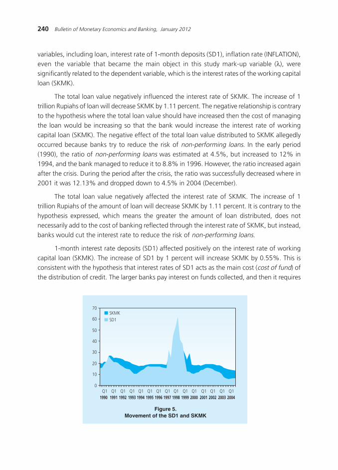
Figure 5.Movement of the SD1 and SKMK
0
10
20
30
40
50
60
70SKMKSD1
1990 1991 1992 1993 1994 1995 1996 1997 1998 1999 2000 2001 2002 2003 2004Q1 Q1 Q1 Q1 Q1 Q1 Q1 Q1 Q1 Q1 Q1 Q1 Q1 Q1 Q1
variables, including loan, interest rate of 1-month deposits (SD1), inflation rate (INFLATION),
even the variable that became the main object in this study mark-up variable (λ), weresignificantly related to the dependent variable, which is the interest rates of the working capital
loan (SKMK).
The total loan value negatively influenced the interest rate of SKMK. The increase of 1trillion Rupiahs of loan will decrease SKMK by 1.11 percent. The negative relationship is contrary
to the hypothesis where the total loan value should have increased then the cost of managing
the loan would be increasing so that the bank would increase the interest rate of workingcapital loan (SKMK). The negative effect of the total loan value distributed to SKMK allegedly
occurred because banks try to reduce the risk of non-performing loans. In the early period
(1990), the ratio of non-performing loans was estimated at 4.5%, but increased to 12% in1994, and the bank managed to reduce it to 8.8% in 1996. However, the ratio increased again
after the crisis. During the period after the crisis, the ratio was successfully decreased where in
2001 it was 12.13% and dropped down to 4.5% in 2004 (December).
The total loan value negatively affected the interest rate of SKMK. The increase of 1trillion Rupiahs of the amount of loan will decrease SKMK by 1.11 percent. It is contrary to the
hypothesis expressed, which means the greater the amount of loan distributed, does not
necessarily add to the cost of banking reflected through the interest rate of SKMK, but instead,banks would cut the interest rate to reduce the risk of non-performing loans.
1-month interest rate deposits (SD1) affected positively on the interest rate of working
capital loan (SKMK). The increase of SD1 by 1 percent will increase SKMK by 0.55%. This isconsistent with the hypothesis that interest rates of SD1 acts as the main cost (cost of fund) of
the distribution of credit. The larger banks pay interest on funds collected, and then it requires
241Market Power of Indonesian Banking
a larger income as well. That is why interest rates of SKMK would increase. This uni-directional
relationship is shown in Figure 5, where the credit interest rate (SKMK) is always higher (exceptin the period of crisis) than the 1-month deposit interest rate, and has a uni-directional movement.
The variable of 1-month interest rate of deposits (SD1) influenced positively on the Interest
Rate of working capital loan (SKMK). The increase by 1 percent on SD1 will increase SKMK by0.55%. This is consistent to the hypothesis that the SD1 interest rate serves as a major cost of
loan distribution. The more banks pay the interest from the collected fund, and then they
require a larger income as well. That is why SKMK interest rates would be increased.
Inflation rate (INFLATION) negatively influenced the interest rates of working capital loan(SKMK), in which each increase of 1 percent Inflation would decrease SKMK by 0.4 percent.
This negative relationship is contrary to the hypothesis, whereby when the inflation rate rises,
the cost of funds collected by banks would increase because the banks receive a repaymentwhich is fewer than the funds distributed at the first time. To prevent it, the banks will increase
the loan interest rate. However, in this paper, the relationship between inflation and loan interest
rates would be negative.
A possible explanation of these results is the existing positive relationship between the
risk of bad debts and the inflation rate. To reduce the risk of bad debts when inflation increases,
the bank should lower the interest rate of the loan. As in the previous description, the ratio ofbad debts was relatively high during the period of analysis and only decreased at the end of the
period of analysis.
Inflation rate (INFLATION) negatively influenced the interest rate of working capital loan(SKMK). It means the increase of INFLATION rate by 1 percent will decrease the SKMK by 0.4
percent.
What became the main object of this study is the level of market power exercised by
Indonesia»s national banks. In constructing the main hypothesis of this study, the market powerin the loan market of the Indonesian banking industry is expected to be high because it has a
high level of concentration. In other words, it estimated that the level of competition in Indonesian
banking industry is relatively low. From the result estimation of the above model, it obtainedthe level of market power (mark-up) by 0.023. With the low level of market power, it proved
that the joint hypotheses which expressed that the empowerment of market power in the
banking loan market was high, which also shows that the relatively low level of competitioncannot be accepted.
The estimation result of market power in the loan market of the Indonesian national
banking industry generated quite a low mark-up value. The table below shows a comparisonof the market power level between loan market of Indonesian banking and hypothetical oligopoly
condition.
242 Bulletin of Monetary Economics and Banking, January 2012
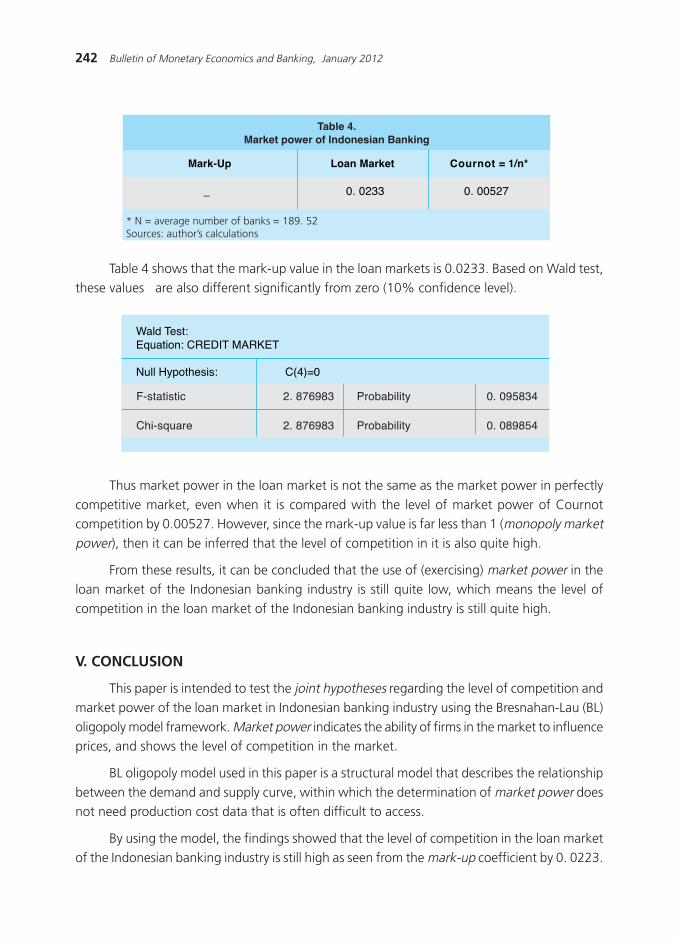
Table 4.Market power of Indonesian Banking
Mark-Up
_ 0. 0233 0. 00527
Loan Market Cournot = 1/n*
* N = average number of banks = 189. 52Sources: author»s calculations
F-statistic 2. 876983 Probability 0. 095834
Chi-square 2. 876983 Probability 0. 089854
Wald Test:Equation: CREDIT MARKET
Null Hypothesis: C(4)=0
Table 4 shows that the mark-up value in the loan markets is 0.0233. Based on Wald test,
these values are also different significantly from zero (10% confidence level).
Thus market power in the loan market is not the same as the market power in perfectly
competitive market, even when it is compared with the level of market power of Cournotcompetition by 0.00527. However, since the mark-up value is far less than 1 (monopoly marketpower), then it can be inferred that the level of competition in it is also quite high.
From these results, it can be concluded that the use of (exercising) market power in theloan market of the Indonesian banking industry is still quite low, which means the level of
competition in the loan market of the Indonesian banking industry is still quite high.
V. CONCLUSION
This paper is intended to test the joint hypotheses regarding the level of competition and
market power of the loan market in Indonesian banking industry using the Bresnahan-Lau (BL)
oligopoly model framework. Market power indicates the ability of firms in the market to influenceprices, and shows the level of competition in the market.
BL oligopoly model used in this paper is a structural model that describes the relationship
between the demand and supply curve, within which the determination of market power doesnot need production cost data that is often difficult to access.
By using the model, the findings showed that the level of competition in the loan market
of the Indonesian banking industry is still high as seen from the mark-up coefficient by 0. 0223.
243Market Power of Indonesian Banking
However, although the level of competition is high, the credit market of the Indonesian banking
industry cannot be said to be a perfectly competitive market.
The study results using BL oligopoly model estimated that the competition level of the
structural equations have different results when compared «measuring» the level of competition
based on the level of banking concentration. Based on the concentration level at the value ofCR4 estimated by 40s, it shows that banking industry remains relatively competitive. However,
with the BL oligopoly model, it is seen that the banking industry in the credit market has
already been relatively competitive.
The study uses the BL oligopoly model that estimates market power directly from thestructural equation, and implies that it is not valid to use market structural data as an indication
of the level of competition in the loan market for the Indonesian banking industry. Even though
the Indonesian banking industry in the loan market is structurally quite concentrated, thecompetitive behavior of commercial banks in distributing credits is quite high.

244 Bulletin of Monetary Economics and Banking, January 2012
Alexander, D. L., 1988. The Oligopoly Solution Tested. Economic Letters 28, 361-364.Amidu, Mohammed, 2006. The Link between Monetary Policy and Banks Lending Behavior:
The Ghanaian Case. Banks and Bank Systems.Vol.1, Issue 4.
Bikker, J., A., 2003. Testing for Imperfect Competition on EU Deposit and Loan Markets withBresnahan»s Market power Model. De Netherlandsche Bank Research Series, Amsterdam.
Bikker, J. A. and K. Haaf, 2002.Competition, Concentration and Their Relationship: An Empirical
Analysis of the Banking Industry. Journal of Banking and Finance 26, 2191-2214.Bresnahan, T. F. , 1982. The oligopoly Solution Concept is Identified. Economics Letters 10, 87-
92.
_____________. , 1989. Empirical Studies in Industries with Market power, In: Schmalensee, R.Willig, R. D. (Eds.), Handbook of Industrial Economics, vol. 2. North-Holland, Amsterdam.
Church, J. , And R. Ware, 2000. Industrial Organization: A Strategic Approach. Boston,Massachusetts, Irwin McGraw-Hill.
Cole, David C. and Betty F. Slade, 1996. Building a Modern Financial System: The IndonesianExperience, Cambridge University Press.
Lau, L. J., 1982. On Identifying the Degree of Competitiveness from Industry Price and Output
Data. Economics Letters 10, 93-99.
Layard P. R. G and Walters, A. A., 1978. Microeconomic Theory. Mac-Graw Hill.Lubis, AndiF. , 1997. Structure and Market power: Analysis of Panel on Processing Industry
from 1985 to 1994. S1 FEUI Thesis (unpublished). Depok.
Norman, G and La Manna, M (eds), 1992. The New Industrial Economics, Aldershot, EdwardElgar.
Panzar, J. and Rosse, J., 1987. Testing for «Monopoly» Equilibrium, Journal of Industrial Economics35, 443-456.
Steen, F. and Salvanes, K. G., 1999. Testing for Market power Using a Dynamic oligopoly
models. International Journal of Industrial Organization 17, 147-177.
Toolsema, L. A., 2002. Competition in the Dutch Consumer Credit Market. Journal of Bankingand Finance 26, 2215-2229.
REFERENCES

245The Impact of Excess Liquidity on Monetary Policy
THE IMPACT OF EXCESS LIQUIDITY ONMONETARY POLICY
M. Barik BathaluddinNur M. Adhi P.Wahyu A.W. 1
This paper analyzes the excess liquidity especially on banking industry and its impact on monetary
policy in Indonesia. We firstly investigate the determinants of bank behavior on their favor for excess
liquidity both for precautionary motive and involuntary. Furthermore we determine the threshold between
the low and high excess liquidity regimes. On the next step, this paper evaluates and compares the impact
of excess liquidity on monetary policy between the two regimes. The first result shows that the excess
liquidity on bank with their precautionary motive is significantly determined by the volatility of money
demand, the volatility of economic growth, the bank cost of the bank, and also by the lag of excess
liquidity, which conform its persistence. Secondly, using the Threshold-VAR approach, this paper shows
the switching regime occurs in 2005 from low to high excess liquidity. Lastly, the excess liquidity reduces
the effectiveness of monetary policy on controlling inflation.
1 M. Barik Bathaluddin ([email protected]), Nur M. Adhi P. ([email protected]), and Wahyu A.W ([email protected]) are researcher onBureau of Economic Research, Directorate of Economic and Monetary Policy Research, Bank Indonesia. We thank to Dr. IskandarSimorangkir, Prof. Dr. Ir. Hermanto Siregar, M.Ec and other researchers for valuable discussion and comments. The view on this paperare solely of the authors and do not necessarily represent any institution.
Abstract
Keywords: Excess liquidity, Threshold VAR, monetary policy transmission mechanism.
JEL Classification: B23, E5
246 Bulletin of Monetary Economics and Banking, January 2012
I. INTRODUCTION
Excess liquidity in Indonesian banking started since economic crisis 1997. At that time,
the worsen condition of national banking due to the high non-performing credit and the decline
in public confidence urged the government to provide liquidity supportfor the troubled banks.The aim was to rescue the entire banking system. However, since the government fund was not
sufficient, in 1998 Bank Indonesia provided bailout fund, known as Bank Indonesia Liquidity
Support (BLBI), by Rp 144.5 trillion. Other programsto save the banking system was bankingrestructuring and recapitalization program. For the latter program, government issued bond
for capital participation in 24 banks, to help them meet the capital requirements ruled by Bank
Indonesia. These two programs; BLBI and banking recapitalization program, started the era ofsoaring and persistent excess liquidity in national banking system, until now.
Along with the economic development, the persistency of excess liquidity often creates
problems for the central bank and for the economy in general. Excess liquidity can reduce the
effectiveness of monetary policy transmission mechanism, especially in affecting demand sideto reachthe targeted inflation. In addition, the excess liquidity in banking system will push the
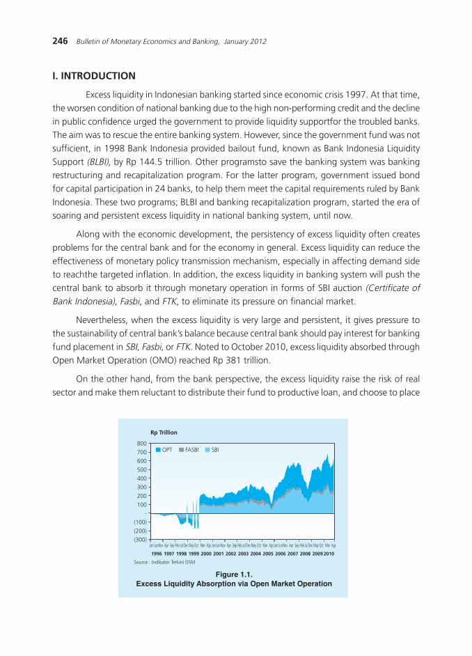
central bank to absorb it through monetary operation in forms of SBI auction (Certificate ofBank Indonesia), Fasbi, and FTK, to eliminate its pressure on financial market.
Nevertheless, when the excess liquidity is very large and persistent, it gives pressure to
the sustainability of central bank»s balance because central bank should pay interest for banking
fund placement in SBI, Fasbi, or FTK. Noted to October 2010, excess liquidity absorbed throughOpen Market Operation (OMO) reached Rp 381 trillion.
On the other hand, from the bank perspective, the excess liquidity raise the risk of real
sector and make them reluctant to distribute their fund to productive loan, and choose to place
Figure 1.1.Excess Liquidity Absorption via Open Market Operation
Rp Trillion
Source : Indikator Terkini DSM
(300)
(200)
(100)
-
100
200
300
400
500
600
700
800
1996 1997 1998 1999 2000 2001 2002 2003 2004 2005 2006 2007 2008 20092010
OPT FASBI SBI
Jan JunNov Apr Sep Feb JulDec May Oct Mar Ags Jan JunNov Apr Sep Feb JulDec May Oct Mar Ags Jan JunNov Apr Sep Feb JulDec May Oct Mar Ags

247The Impact of Excess Liquidity on Monetary Policy
it in monetary instrument. Consequently, the fund for the real sector is limited and even if it is
available, the price would be higher.
However, not all excess liquidity portions negativelyaffect the effectiveness of monetary
policy transmission mechanism. In certain portion, excess liquidity is useful as a buffer for banking
towards the uncertainty of fund withdrawal by customer and exchange rate volatility, influencethe banking capital. Within this necessaryportion, excess liquidity is called precautionary excessliquidity. The remaining excess liquidity is unnecessary and is potential to give negative impacts
for effectiveness of monetary policy. This remaining excess liquidity is called involuntary excessliquidity.
Therefore, it is necessary to determine the magnitude of precautionary and involuntary
excess liquidity. By having this knowledge, authority monetary can determine how much excess
liquidity to absorb through open market operations (OMO).
Empirical research on excess liquidity and its consequences toward the effectiveness of
monetary policy are widely available. Saxegaard (2006)2is one of the most cited references.
Saxegaard underline the necessity to quantify how much excess liquidity needed by bankingfor precautionary purpose. Using the sample of African countries in Sahara, he found that
significant amount of involuntary excess liquidity reducedthe effectiveness of monetary policy
transmission in controlling inflation. The reason is better aggregate demand increase the lendingrapidly, and then increases the risk of inflation pressure.
Absorbing excess liquidity through OMO is expensive for the central bank. On the other
hand, during cyclical downturn condition, stimulating aggregate demand would be ineffectivesince banking cannot put this unproductive excess liquidity in the form of lending or treasury
bills.
Following Saxegaard method(2006), this paper will (i) calculateprecautionary and
involuntary excess using banking excess liquidity model; (ii) estimate regime-switching modelsof monetary policy transmission mechanism, using threshold-VAR to determine the regime
period of high and low precautionary excess liquidity.In general, the objectives of this research
areto acknowledge the impact of excess liquidity persistency on monetary policyeffectiveness; and to give policy recommendation toward excess liquidity persistency
condition.
The second session of this paper covers theories and literature studies. The third sessioncovers methodology and data, while the fourth session analyzes the result and analysis.
Conclusion will be given in the last session part and close the presentation.
2 Magnus Saxegaard, IMF Working Paper, WP/06/115: Excess Liquidity and Effectiveness of Monetary Policy: Evidence from Sub-Saharan Africa.
248 Bulletin of Monetary Economics and Banking, January 2012
R + L = D
II. THEORY
Excess liquidity is the bankΩreserves deposited in central bank, plus cash for daily operational
needs (cash in vaults), minus minimum reserve requirement, (Saxegaard, 2006). In this context,
excess liquidity is used by banks as a precautionary, and representing the bank optimizationbehavior.
The sources of precautionary excess liquidity can be varied. Crisis with high uncertainty
and high default risk can be one of them, where banking tends to keep non-remunerated
liquid assets as precautionarystrategy (Agenor et.al, 2004). Another source of excess liquidity isinstitutional factor, where under developed interbank money market (IBM) will stimulate bank
to increase liquidity for precautionary, since they often find it hard to borrow in emergency
situation. Two other sources of excess liquidity are the difficulty on watching their minimumreserve requirement position; therefore the banks will hold reserves above the level set, and
also the problems in payment system.
Not all excess liquidity arises from bank precautionary behavior. In a certain condition,excess liquidity owned by banks is neither precautionary nor involuntary. In this involuntary
context, non-remunerated reserves owned by banks do receive return to balance the opportunity
cost when it is held by banks.
Banks prefer holding excess liquidity than giving loan or buy government obligation,
especially in a long run. The reason is the economic condition is in liquidity trap. Liquidity trap
is a condition where return from banking credit is too small to cover intermediation cost andbanks get higher yield in reserves than giving loans. In this condition, expansive monetary
policy will only cause increase in excess reserves.
Agenor et.al. (2000) developed theoretical model of excess liquid reserves demandby
commercial banks, where liquidity and volatility risks of real sector exist. To manage both ofthese risks, and to determine the amount liquid assets to hold, commercial banks can get fund
from interbank money market or from the central bank.
There is one representative commercial bank that collect exogenous fund from thirdparties (Deposit, D). The bank has to determine the amount of non-interest-bearing liquid asset
(reserve, R) and the amount of interest-bearing non-liquid asset (in credit form, L). The balance
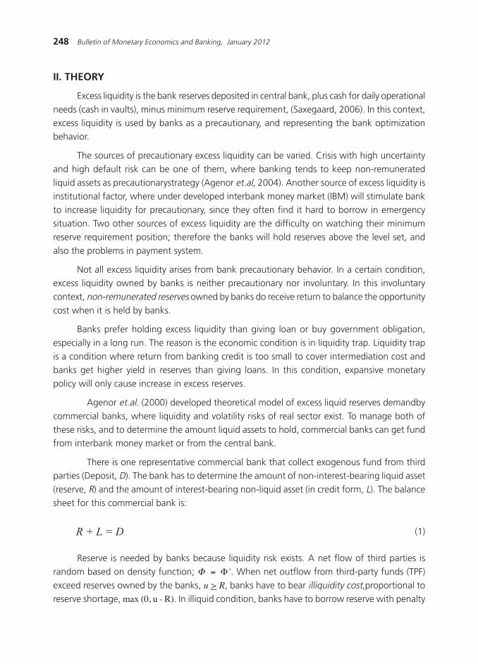
sheet for this commercial bank is:
(1)
Reserve is needed by banks because liquidity risk exists. A net flow of third parties israndom based on density function; Φ = Φ’. When net outflow from third-party funds (TPF)
exceed reserves owned by the banks, u > R, banks have to bear illiquidity cost,proportional to
reserve shortage, max (0, u - R). In illiquid condition, banks have to borrow reserve with penalty
249The Impact of Excess Liquidity on Monetary Policy
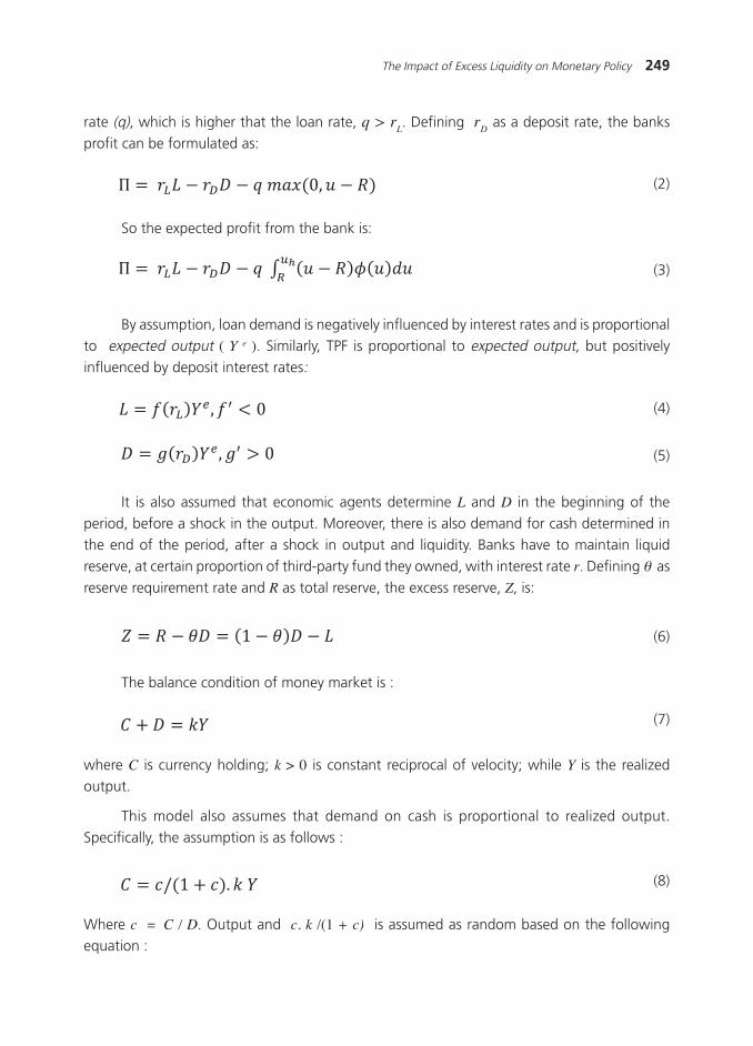
rate (q), which is higher that the loan rate, q > rL. Defining r
D as a deposit rate, the banks
profit can be formulated as:
(2)
By assumption, loan demand is negatively influenced by interest rates and is proportionalto expected output ( Y e ). Similarly, TPF is proportional to expected output, but positively
influenced by deposit interest rates:
(3)
(4)
So the expected profit from the bank is:
(5)
It is also assumed that economic agents determine L and D in the beginning of the
period, before a shock in the output. Moreover, there is also demand for cash determined inthe end of the period, after a shock in output and liquidity. Banks have to maintain liquid
reserve, at certain proportion of third-party fund they owned, with interest rate r. Defining θ as
reserve requirement rate and R as total reserve, the excess reserve, Z, is:
(6)
The balance condition of money market is :
(7)
where C is currency holding; k > 0 is constant reciprocal of velocity; while Y is the realizedoutput.
This model also assumes that demand on cash is proportional to realized output.
Specifically, the assumption is as follows :
(8)
Where c = C / D. Output and c. k /(1 + c) is assumed as random based on the followingequation :

250 Bulletin of Monetary Economics and Banking, January 2012
,
(9)
(10)
(11)
(12)
),,(+−+
= σθqZZ (13)
Where ε and ξ are random shocks.
By applying equations (8) and (9), a demand on cash is formulated as :
To fulfill the needs of unanticipated demands for cash, banks can borrow cash followed byinterest by q, and take some of the excess reserve (Z). By using equation (6), the expected
reserve deficiency is :
Based on equation (11), (4), (5), and (7), we can get the equation for expected profit
from banks as follows :
By assumption, the functions and are quasi-concave functions. We can prove the following
prepositions (the complete proofs can be seen on Agenor et. al, 2000).1. The increase of penalty rate (q) will increase the deposit interest rates, credit interest rates
and excess reserve owned by banks.
2. The increase of output»s volatility and liquidity shock causes ambiguous effects to depositinterest rates,»loan»interest rates, and excess reserve. If the initial level of penalty rate is
pretty high, the increase of this volatility will also rise up the deposit interest rates, loan
interest rates, and excess reserve.3. The increase of reserve requirement rate will increase the credit interest rates and decrease
excess reserve. If the level of volatility is not too high, an increase of reserve requirement
rate will increase the deposit interest rates.
Based on the three prepositions above, if the level of penalty rate is high, there will beinterrelationship among excess reserve (z), penalty rate (q), reserve requirement rate (θ), and
output»s volatility and liquidity shock ( σ ) as follows :

251The Impact of Excess Liquidity on Monetary Policy
By sorting excess liquidity into the precautionary and the involuntary, we have deeper
understandings about their impact on the monetary policy transmission mechanism. Oninflationary contexts, involuntary excess liquidity will be released promptly when the
aggregate demand side grows stronger. Therefore, the total liquidity in economy will
increase rapidly without involving policy rate reduction mechanism (loosen monetarypolicy), just when the liquidity should be restricted. This triggers the risk of inflation
pressure.
Furthermore, when banking has involuntary excess liquidity due to the problem indistributing loan, an effort to increase the demand by decreasing the lending cost would be
ineffective. The expansive monetary policy will only increase the excess reserve in banks and
not the loan expansion. In contrast, if tight monetary policies are chosen, banks will reducetheir unwanted reserve. O»Connell (2005)3 states that :
≈ When there is involuntary excess liquidity in the economy in equilibrium, the transmission
mechanism of monetary policy, which usually runs from a tightening or loosening of liquidity
conditions to changes in interest rates or asset demands and then to economic activity, is altered
and possibly interrupted completely. º.∆
On the other hand, monetary policy is expected to be more effective if banks have
the precautionary liquidity access. For example, when monetary policy is loosening by
decreasing minimum reserve requirement, bank liquidity will rise; hence will increase theallocation for loanwith lower interest rate. On the other hand, when the central bank
choosestight monetary policy, banking will reduce their loans to maintain the level of
expected excess reserve.
Based on the descriptions above, the analysis on the effects of excess liquidity to monetary
policy transmission mechanism requires better understanding on how consistent the policy on
reserve requirement is, on driving the excess reserve demand of bank. Moreover, theunderstanding on the sources of excess liquidity is important to decide what policy should be
taken.
There have been a lot of researches about excess liquidity in Indonesia. They focus on
different views about source and impact of the excess liquidity. Some of the researches aresummarized in the table below.
3 Stephen O»Connell, 2005, ≈A Floor and Ceiling Model of U.S. Output,∆ Journal of Economics Dynamic and Control, Vol. 21, pp.661-95.
252 Bulletin of Monetary Economics and Banking, January 2012
ln ln ln
III. METHODOLOGY
3.1. Estimation of Precautionary and Involuntary Excess Reserve
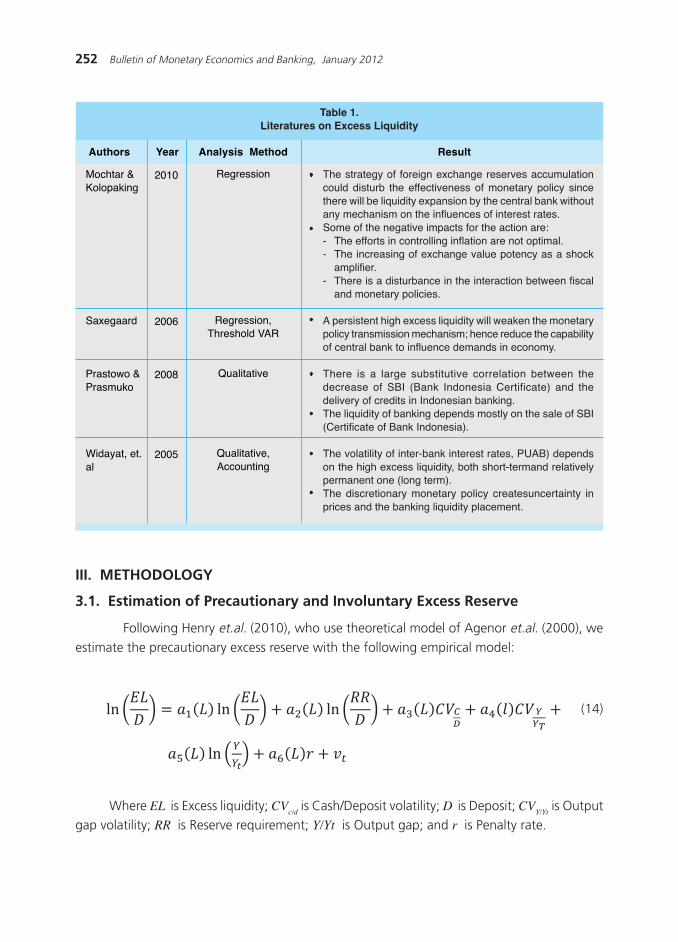
Following Henry et.al. (2010), who use theoretical model of Agenor et.al. (2000), we
estimate the precautionary excess reserve with the following empirical model:
Table 1.Literatures on Excess Liquidity
Authors Year Analysis Method Result
Mochtar &Kolopaking
Saxegaard
Prastowo &Prasmuko
Widayat, et.al
2010
2006
2008
2005
Regression
Regression,Threshold VAR
Qualitative
Qualitative,Accounting
- The strategy of foreign exchange reserves accumulationcould disturb the effectiveness of monetary policy sincethere will be liquidity expansion by the central bank withoutany mechanism on the influences of interest rates.Some of the negative impacts for the action are:- The efforts in controlling inflation are not optimal.- The increasing of exchange value potency as a shock
amplifier.- There is a disturbance in the interaction between fiscal
and monetary policies.
A persistent high excess liquidity will weaken the monetarypolicy transmission mechanism; hence reduce the capabilityof central bank to influence demands in economy.
There is a large substitutive correlation between thedecrease of SBI (Bank Indonesia Certificate) and thedelivery of credits in Indonesian banking.The liquidity of banking depends mostly on the sale of SBI(Certificate of Bank Indonesia).
The volatility of inter-bank interest rates, PUAB) dependson the high excess liquidity, both short-termand relativelypermanent one (long term).The discretionary monetary policy createsuncertainty inprices and the banking liquidity placement.
(14)
Where EL is Excess liquidity; CVc/d
is Cash/Deposit volatility; D is Deposit; CVY/Yt
is Outputgap volatility; RR is Reserve requirement; Y/Yt is Output gap; and r is Penalty rate.

253The Impact of Excess Liquidity on Monetary Policy
We use Certificate of Bank of Indonesia (SBI) owned by bank as the proxy for excess
liquidity. This is in line with Prastowo and Prasmoko (2008), which argue that banks prefer toput their excess liquidity in the form of SBI rather than in giral account in Bank Indonesia. We
use monthly data as listed on the following table:
Table 2.Data for Precautionary and Involuntary Excess Liquidity Estimation
Variable Source of Data
Excess Liquidity
Third Party Funds
Reserve Requirement
Coefficient of variation of Cash to depositratio (volatility risk)
Coefficient of variation of output from trend
Penalty rate
Output Gap (proxy for demand for Cash)
Monetary Survey - Volume of SBI which own by banks
Monetary Survey
CEIC
Moving average from standard deviation of cash ratio to
Deposit (5 month). Cash and Deposit datawere from
monetary survey
Moving average from standard deviation of output gap
(5 month)
Interest rate PUAB o/n (CEIC)
Outputis represented with Industrial Production (CEIC).
Potential output is estimated using HP Filter.
After estimatingprecautionary excess reserve using Equation (13), we proceed to estimating
involuntary excess reserve. In this step, we subtract the actual independent variables in Equation(13), which were the proxy for total excess liquidity owned by banks, with the estimated one
from Equation (13). In the other words, involuntary excess reserve is estimated with residual
from Equation (13) estimation.
3.2. The Impact of Involuntary Excess Reserve on Monetary PolicyTransmission
On this step, we test the hypothesis; that the presence of high involuntary excess reserve
in banking may weaken the monetary policy transmission mechanism. Following Saxegaard(2006), we use estimated involuntary excess reserve from the first step as a threshold variable in
analyzing VAR model, which represent the transmission of monetary policy in Indonesia. In this
stage, we allow the possibility for non-linearity in monetary policy transmission caused bydeviation of involuntary excess liquidity relative to certain threshold.

254 Bulletin of Monetary Economics and Banking, January 2012
Where and are shock vectors that are not regime dependent, representing non-
policy and policy variable respectively; is regime-dependent matrix of polynomial lag
from autoregressive parameter; is threshold variable(involuntary excess reserve), which
determine the current regime, relative to certain threshold ( τ ).
As in Bernanke and Milhov (1995), the dependent variables are divided into two groupin
reduced form VAR; non-policy variable such as GDP and inflation, and policy variable including
nominal exchange rate and BI rate policy. The data we useon this step is explained in Table 3.All variables are transformed into natural logarithm and are de-trended using HP Filter.
(15)
We estimate the reduced form two-regime TVAR below:
Table 3.Data for ThresholdVAR Estimation
Variable Source of Data
Involuntary Excess liquidity
Output
Inflation (yoy)
Exchange rate
BI rate
Estimated from step 1
Industrial production (CEIC)
Source: DSM
Source: CEIC
Source: DSM
In estimating this reduced form VAR, we apply MSVAR software (Krolzig-1998). The
existence of non-linearity in monetary policy transmission mechanism will formally be tested
using this program. Furthermore, regime-dependent impulse response will be used to analyzethe difference of economics response towards monetary policy shock between the 2 regimes.
Christiano and Echenbaum (1996) argue that one cannot identify the impact of monetary
policy shock directly using the reduced form two-regime TVAR model in Equation (14), sincethe covariance matrix of residual vector is not diagonal. This is because the monetary policy
depends on economic condition;hence response of the economic variable reflects the
combination effect between monetary policy and other variables which also changethe monetary
255The Impact of Excess Liquidity on Monetary Policy
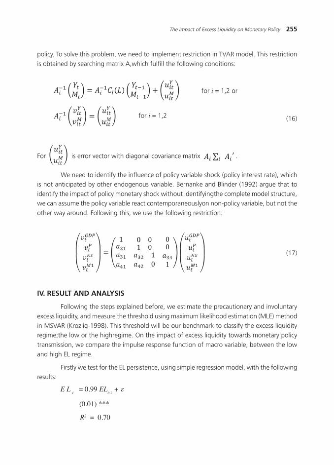
policy. To solve this problem, we need to implement restriction in TVAR model. This restriction
is obtained by searching matrix A,which fulfill the following conditions:
For is error vector with diagonal covariance matrix .
We need to identify the influence of policy variable shock (policy interest rate), whichis not anticipated by other endogenous variable. Bernanke and Blinder (1992) argue that to
identify the impact of policy monetary shock without identifyingthe complete model structure,
we can assume the policy variable react contemporaneouslyon non-policy variable, but not theother way around. Following this, we use the following restriction:
(16)
for i = 1,2 or
for i = 1,2
(17)
IV. RESULT AND ANALYSIS
Following the steps explained before, we estimate the precautionary and involuntary
excess liquidity, and measure the threshold using maximum likelihood estimation (MLE) method
in MSVAR (Krozlig-1998). This threshold will be our benchmark to classify the excess liquidityregime;the low or the highregime. On the impact of excess liquidity towards monetary policy
transmission, we compare the impulse response function of macro variable, between the low
and high EL regime.
Firstly we test for the EL persistence, using simple regression model, with the following
results:
E L t = 0.99 EL
t-1 + ε
(0.01) ***
R2 = 0.70
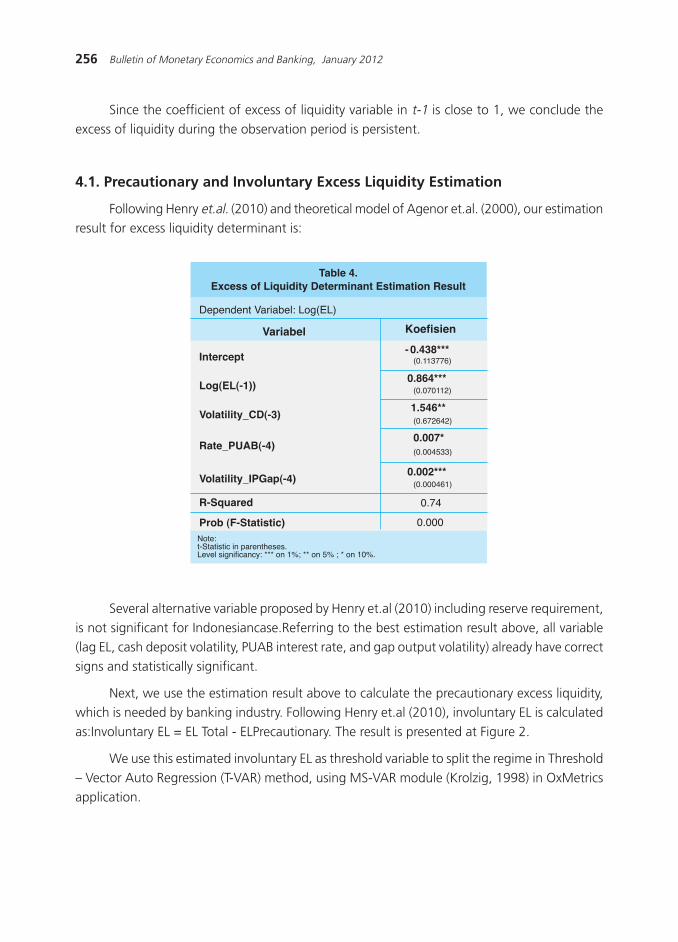
256 Bulletin of Monetary Economics and Banking, January 2012
Since the coefficient of excess of liquidity variable in t-1 is close to 1, we conclude the
excess of liquidity during the observation period is persistent.
4.1. Precautionary and Involuntary Excess Liquidity Estimation
Following Henry et.al. (2010) and theoretical model of Agenor et.al. (2000), our estimationresult for excess liquidity determinant is:
Table 4.Excess of Liquidity Determinant Estimation Result
Dependent Variabel: Log(EL)
Variabel Koefisien
Intercept- 0.438***
(0.113776)
Log(EL(-1))0.864***
(0.070112)
Volatility_CD(-3)1.546**(0.672642)
Rate_PUAB(-4)0.007*(0.004533)
Volatility_IPGap(-4)0.002***
(0.000461)
R-Squared 0.74
Prob (F-Statistic) 0.000Note:t-Statistic in parentheses.Level significancy: *** on 1%; ** on 5% ; * on 10%.
Several alternative variable proposed by Henry et.al (2010) including reserve requirement,
is not significant for Indonesiancase.Referring to the best estimation result above, all variable(lag EL, cash deposit volatility, PUAB interest rate, and gap output volatility) already have correct
signs and statistically significant.
Next, we use the estimation result above to calculate the precautionary excess liquidity,which is needed by banking industry. Following Henry et.al (2010), involuntary EL is calculated
as:Involuntary EL = EL Total - ELPrecautionary. The result is presented at Figure 2.
We use this estimated involuntary EL as threshold variable to split the regime in Threshold
√ Vector Auto Regression (T-VAR) method, using MS-VAR module (Krolzig, 1998) in OxMetricsapplication.

257The Impact of Excess Liquidity on Monetary Policy
4.2. Excess Liquidity Threshold and Regime Classification
T-VAR estimation refers to Saxegaard (2006) and Bernanke and Blinder (1992), using 4
endogenous variables; namely Production Index (GDP proxy), Inflation, Exchange Rate, and BIRate. Production Index and Inflation variable are non-policy variable, while Exchange Rate and
Figure 2.Excess Liquidity: Precautionary vs. Involuntary
2000 2001 2002 2003 2004 2005 2006 2007 2008 2009 2010-.04
.00
.04
.08
.12
.16
.20_ELTOTAL _ELPREC _ELINV
SETAR, 2001 (10) - 2010 (9)
Probabilities of Regime 1
Probabilities of Regime 2
2002 2003 2004 2005 2006 2007 2008 2009 2010
2002 2003 2004 2005 2006 2007 2008 2009 2010
2002 2003 2004 2005 2006 2007 2008 2009 2010
-5
0
5
10
0.5
1.0
0.5
1.0
IP
ER
Inf_y
BIRate_R
Figure 3.Involuntary Excess Liquidity Regime: Low vs. High

258 Bulletin of Monetary Economics and Banking, January 2012
Table 5.Estimated Threshold Value with MLE Method
Estimated Threshold
LR Test
p-values (adjusted χχχχχ2)
0.00048870
Low 2001:08 - 2005:9
High 2005:10 - 2010:9
237.7847
[0.0000]
Rezim Classification
BI Rate variable are policy variable. Again, policy variable react contemporaneously on non-
policy variable, but not the other way around. In addition, we adjustthe S-VAR structure byincluding NFA variable as exogenous variable, to suit the condition for Indonesia.NFA is also
policy variable, and potentially affects the exchange rate and inflation.
The result of T-VAR estimation is presented below. Complete result is provided inAppendix A.
We try several lag alternatives (from lag 0 to 8) for the threshold variable (EL variable),
and found lag 2to be the best choice because it provide more intuitive result. In addition, it
suits the economic condition break in 2005 due to inflation hike, a high BI rate, and reserverequirement policy.
During the period from October 2001 - September 2009, we found two excess liquidity
regime; low EL Regime for August 2001-September 2005, and high EL Regime for October2005√September 2010. Using maximum likelihood estimation (MLE) in MS-VAR module, the
estimated threshold is:
The Likelihood Ratio (LR) above is important to test the linearity of EL threshold withinthe sample range 2001:8 to 2010:9. According to that result, high LR coefficient value (237.7847)
and p-values (below 5%) confirms nonlinearity on EL, hence support our EL regime classification.
4.3. The Impact of Excess Liquidity on Monetary Policy
We use policy rate as the proxy for monetary policy and analyze its effectiveness toward
other macro variables such as production index (GDP proxy), inflation and exchange rate. On
VAR structure, we evaluate the monetary policy transmission by giving one standard deviationshock (impulse) on BI rate, then compare its impact on the two classified regime. The result is
presented below.
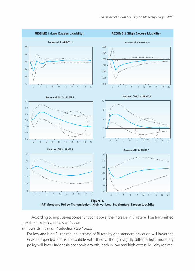
259The Impact of Excess Liquidity on Monetary Policy
Figure 4.IRF Monetary Policy Transmission: High vs. Low Involuntary Excess Liquidity
REGIME 1 (Low Excess Liquidity) REGIME 2 (High Excess Liquidity)
Response of IP to BIRATE_R
-.12
-.08
-.04
.00
.04
.08
2 4 6 8 10 12 14 16 18 20
Response of INF_Y to BIRATE_R
-1.5
-1.0
-0.5
0.0
0.5
1.0
1.5
2 4 6 8 10 12 14 16 18 20
Response of ER to BIRATE_R
-.06
-.04
-.02
.00
.02
.04
2 4 6 8 10 12 14 16 18 20
Response of IP to BIRATE_R
-.100
-.075
-.050
-.025
.000
.025
.050
2 4 6 8 10 12 14 16 18 20
Response of INF_Y to BIRATE_R
-4
0
4
8
12
2 4 6 8 10 12 14 16 18 20
Response of ER to BIRATE_R
-.20
-.15
-.10
-.05
.00
.05
.10
2 4 6 8 10 12 14 16 18 20
According to impulse-response function above, the increase in BI rate will be transmitted
into three macro variables as follow:a) Towards Index of Production (GDP proxy)
For low and high EL regime, an increase of BI rate by one standard deviation will lower the
GDP as expected and is compatible with theory. Though slightly differ, a tight monetarypolicy will lower Indonesia economic growth, both in low and high excess liquidity regime.
260 Bulletin of Monetary Economics and Banking, January 2012
b) Towards Inflation
During low EL regime (left picture), an increase of BI rate will reduce the inflation pressure,which is in line with Inflation Targeting Framework (ITF). Though it needs few lags for the
inflation to response the policy rate, the interest-based policy performs fairly well on this
regime. Nevertheless, we do not find condition during high EL regime (right picture).Interestingly, when economic is in high excess liquidity, the monetary policy transmission is
not effective to restrains inflation. In fact, in high EL regime, an increase of BI rate is responded
with an increase of inflation.One possible explanation is that over accelerated economic needs to be responded with an
increase of BI rate, which reduce the fund on market. However, in high excess liquidity
regime, the public fund remains largely available; hence the demand will be relatively highercompared to low EL regime.
This positive relationship between BI rate and inflation require further research. As for current
paper, we only focus on comparison between the two regimes, and conclude that the highexcess liquidity in economics will lower the effectiveness of BI rate to control inflation.
c) Towards exchange rate
In line with the uncovered interest parity (UIP) theory, the increase of BI rate will raise thevalue of IDR. An increase of domestic interest rate will make domestic more attractive,
therefore increase the demand for IDR. This result applies for both low and high EL regime.
The analysis of impulse response function above is based on SVAR structure with thefollowing endogenous variables: Index of Production, Inflation, Exchange rate, BI rate, and NFA
(Net Foreign Assets). As additional analysis and comparison, we specify two alternatives of
SVAR structure namely alternative A which only include Index of Production, Inflation, Exchangerate, and BI rate variables, and exclude NFA. However the result of this pure structure from
Bernanke and Blinder (1992), give inconclusive result and does not consistent with the theory.
Alternative B, we use Non-Performing Loan (NPL) variable to capture the constraint on loansupply. Likewise, this alternative also does not provide conclusive result. We report the complete
result for both alternatives on appendix.
In general, we have shown that excess liquidity affect the effectiveness of monetarypolicy. In high EL regime condition, the impact of BI rate as a monetary policy instrument in
order to reach the monetary policy objective (which is low and stable inflation), is relatively
lower than in low EL regime. Therefore, several initiative programs of Bank Indonesia related tocontrolling and managingliquidity are necessary and require further improvement.
V. CONCLUSION
This paper gives several important conclusions. First, the behavior of bank to keep excessliquidity for precautionary is affected significantly by the volatility of cash demand, the volatility

261The Impact of Excess Liquidity on Monetary Policy
of economic growth, the cost of fund for bank, and the liquidity condition in previous period.
Second, the application of Threshold-VAR (TVAR) method shows that there are two regimesof excess liquidity in Indonesia; the Low EL Regime (2001:08 √ 2005:9) and√the High EL Regime
(2005:10 √ 2010:9). The regime switch occurred in 2005, when there were significant changes
in Indonesia economics condition including the increases of inflation, BI Rate, higher openmarket operation, policy changeon minimum reserve requirement, and also the rise of foreign
reserve accumulation in Bank Indonesia.
The policy implication is straightforward. Bank Indonesia needs to control and to direct
the high excess liquidity condition. Further endorsement on several existing programs is necessary,including the conversion of SUP (Surat Utang Pemerintah) to be tradable, Treasure Single Account
(TSA) with Asset Liability Management (ALM), and the use of SPN (Surat Perbendaharaan Negara)
as monetary instrument.
This paper calls for further research, especially related to structure of SVAR, which only
consists of 4-5 variables.The model proposed by Bernanke and Blinder (1992) may be appropriate
for developed countries because of the stability of their institutional economics. On the otherhand, Indonesia is a transition country, where the policy is often adjusted to economic situation
and sometimes to the political situation. Therefore, future study should account for this issue,
using the T-VAR method.
262 Bulletin of Monetary Economics and Banking, January 2012
Ben S. Bernanke and Ilian Mihov, 1995, ≈Measuring Monetary Policy∆, NBER Working Papers
5145, National Bureau of Economic Research, Inc.
Bernanke, Ben S and Blinder, Alan S, 1992, ≈The Federal Funds Rate and the Channels ofMonetary Transmission∆,American Economic Review, American Economic Association, vol.
82(4), pages 901-21, September.
Bureau of Economic Research, 2008, ≈Menghadapi Ekses Likuiditas dalam Rangka MeningkatkanEfektivitas Kebijakan Moneter∆, Miemo.
Henry et. al, 2010, ≈The Dynamics of Involuntary Commercial Bank»s Reserves in Trinidad and
Tobago∆, 42nd Annual Monetary Studies Conference Financial Stability, Crisis Preparednessand Risk Management in the Caribbean.
Kiki NindyaAsih, 2005, ≈Telaah Sederhana Kondisi Likuiditas Perbankan dan Implikasi Kebijakan,∆
Ulasan Pojok, vol II No. 10, Juni.Krolzig, Hans-Martin, 1998, ≈Econometric Modeling of Markov-Switching Vector
Autoregressions using MSVAR for Ox∆(unpublished:Oxford, United Kingdom:University of
Oxford).Lawrence J. Christiano, Martin EichenbaumandCharles L. Evans, 1998, ≈Monetary Policy Shocks:
What Have We Learned and to What End?∆, NBER Working Papers 6400, National Bureauof Economic Research, Inc.
Magnus Saxegaard, 2006, ≈Excess Liquidity and the Effectiveness of Monetary Policy: Evidence
from Sub-Saharan Africa∆, IMF Working Papers 06/115, International Monetary Fund.
N. Joko Prastowo and Andry Prasmuko, 2008, ≈Penurunan Portfolio SBI, Pertumbuhan Kreditand Kondisi Likuiditas Perbankan,∆ Mimeo.
P.R. Agenor, J. AizenmanandA. Hoffmaister, 2000, ≈The Credit Crunch in East Asia: What can
Bank Excess Liquid Assets Tell us?∆mNBER Working Papers 7951, National Bureau ofEconomic Research, Inc.
Stephen O»Connell, 2005, ≈A Floor and Ceiling Model of U.S. Output∆, Journal of EconomicsDynamic and Control, Vol. 21, pp. 661-95.
REFERENCES
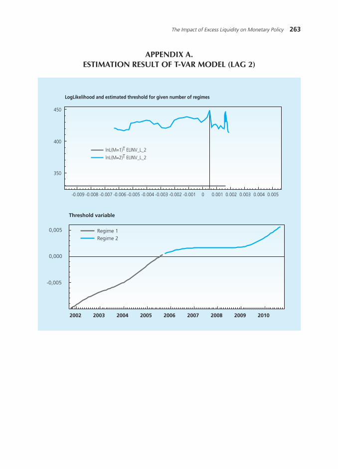
263The Impact of Excess Liquidity on Monetary Policy
APPENDIX A.ESTIMATION RESULT OF T-VAR MODEL (LAG 2)
LogLikelihood and estimated threshold for given number of regimes
350
400
450
-0.009 -0.008 -0.007 -0.006 -0.005 -0.004 -0.003 -0.002 -0.001 0 0.001 0.002 0.003 0.004 0.005
lnL(M=1)T ELINV_L_2
lnL(M=2)T ELINV_L_2
Threshold variable
-0,005
0,000
0,005 Regime 1Regime 2
2002 2003 2004 2005 2006 2007 2008 2009 2010

264 Bulletin of Monetary Economics and Banking, January 2012
Correlogram: Standard resids
0
1ACF-IPPACF-IP
1 13 25
Density : Standard resids
0,25
0,50
-2,5 2,5
IP
N (s=1)
QQ Plot : Standard resids
-2,5
0,0
2,5IP T normal
-2 0 2
Correlogram : Standard resids
0
1
1 13 25
ACF-Inf_yPACF-Inf_y
Spectral density : Standard resids
Inf_y
0,1
0,2
0,3
0,0 0,5 1,0
Density : Standard resids
0.25
0.50
Inf_yN(s=1)
-2.5 0.0 2.5
QQ Plot : Standard resids
-2,5
0,0
2,5
-2 0 2
Inf_y T normal
Spectral density: Standard resids
IP
0,1
0,2
0,0 0,5 1,0
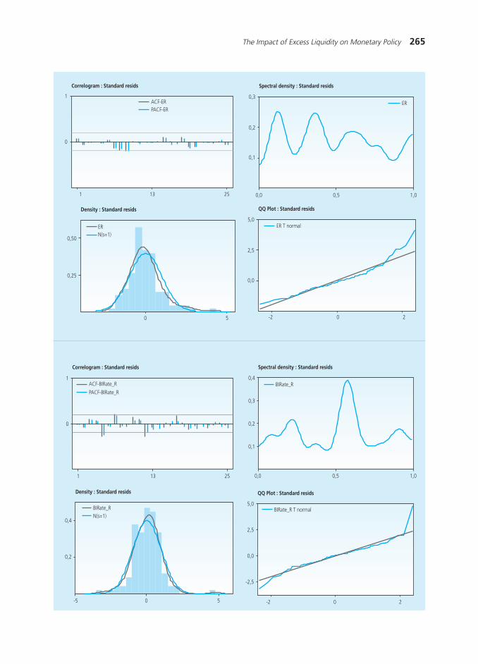
265The Impact of Excess Liquidity on Monetary Policy
Correlogram : Standard resids
0
1ACF-ERPACF-ER
1 13 25
Spectral density : Standard resids
ER
0,1
0,2
0,3
0,0 0,5 1,0
Density : Standard resids
0,25
0,50
0 5
ERN(s=1)
QQ Plot : Standard resids
0,0
2,5
5,0
-2 0 2
ER T normal
Correlogram : Standard resids
0
1
1 13 25
ACF-BIRate_R
PACF-BIRate_R
Spectral density : Standard resids
0,1
0,2
0,3
0,4BIRate_R
0,0 0,5 1,0
Density : Standard resids
0,2
0,4
-5 0 5
BIRate_RN(s=1)
QQ Plot : Standard resids
-2,5
0,0
2,5
5,0
-2 0 2
BIRate_R T normal

266 Bulletin of Monetary Economics and Banking, January 2012
APPENDIX B. IRF SVAR
IRF ALTERNATIVE A:SVAR WITHOUT NFA
REGIME 1 (Low EL) REGIME 2 (High EL)
Response of IP to BIRATE_R
-.12
-.08
-.04
.00
.04
2 4 6 8 10 12 14 16 18 20
Response of INF_Y to BIRATE_R
-1.0
-0.5
0.0
0.5
1.0
1.5
2.0
2 4 6 8 10 12 14 16 18 20
Response of ER to BIRATE_R
-.04
-.02
.00
.02
.04
.06
12 202 4 6 8 10 14 16 18
Response of IP to BIRATE_R
-.12
-.08
-.04
.00
.04
2 4 6 8 10 12 14 16 18 20
Response of INF_Y to BIRATE_R
-10
-5
0
5
10
15
2 4 6 8 10 12 14 16 18 20
Response of ER to BIRATE_R
-.12
-.08
-.04
.00
.04
.08
.12
2 4 6 8 10 12 14 16 18 20
Response to Nonfactorized One S.D.Innovations + 2 S.E.
Response to Nonfactorized One S.D.Innovations + 2 S.E.
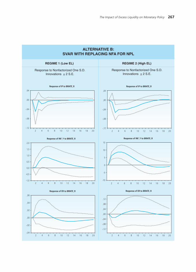
267The Impact of Excess Liquidity on Monetary Policy
ALTERNATIVE B:SVAR WITH REPLACING NFA FOR NPL
REGIME 1 (Low EL) REGIME 2 (High EL)
Response to Nonfactorized One S.D.Innovations + 2 S.E.
Response to Nonfactorized One S.D.Innovations + 2 S.E.
Response of IP to BIRATE_R
-.12
-.08
-.04
.00
.04
2 4 6 8 10 12 14 16 18 20
Response of INF_Y to BIRATE_R
-1,0
-0,5
0,0
0,5
1,0
1,5
2,0
2 4 6 8 10 12 14 16 18 20
Response of ER to BIRATE_R
-,04
-,02
,00
,02
,04
,06
2 4 6 8 10 12 14 16 18 20
Response of IP to BIRATE_R
-,12
-,08
-,04
,00
,04
2 4 6 8 10 12 14 16 18 20
Response of INF_Y to BIRATE_R
-10
-5
0
5
10
15
2 4 6 8 10 12 14 16 18 20
Response of ER to BIRATE_R
-,12
-,08
-,04
,00
,04
,08
,12
2 4 6 8 10 12 14 16 18 20

268 Bulletin of Monetary Economics and Banking, January 2012
This page is intentionally left blank
269Transmission Channel and Effectiveness of Dual Monetary Policy In Indonesia
TRANSMISSION CHANNEL AND EFFECTIVENESS OFDUAL MONETARY POLICY IN INDONESIA
Ascarya 1
This paper investigates the transmission mechanism of dual monetary system from conventional
and Islamic policy rates to inflation and output. We apply Granger Causality and VAR methods on monthly
data of Indonesian banking, during the period of January 2003 to December 2009. The result shows that
conventional policy rate is transmitted to output and inflation, while Islamic policy rate are not. In addition,
the shock of conventional interest rate, credit and interbank rate give a negative and permanent impacts
on inflation and output, except for SBI (Certificate of Bank Indonesia) with positive impact to inflation
though negativelyaffect the output. On the other hand, the shock of PLS, financing and Islamic interbank
PLS, as well as SBIS (Central Bank Shariah Certificate) give positive and permanent impacts on inflation
and output.
Keywords: Monetary transmission mechanism, Interest rate pass through, Conventional Banking,
Islamic Banking
JEL Classification: E43, E52, G21, G28
1 Researcher on PPSK √ Bank Indonesia; [email protected]. The views on this paper are solely of the author and not necessarily representthe views of Bank Indonesia. Author thanks to anonymous referees and the editors, for their constructive discussion.
Abstract
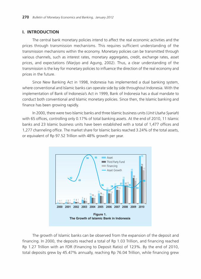
270 Bulletin of Monetary Economics and Banking, January 2012
I. INTRODUCTION
The central bank monetary policies intend to affect the real economic activities and the
prices through transmission mechanisms. This requires sufficient understanding of the
transmission mechanisms within the economy. Monetary policies can be transmitted throughvarious channels, such as interest rates, monetary aggregates, credit, exchange rates, asset
prices, and expectations (Warjiyo and Agung, 2002). Thus, a clear understanding of the
transmission is the key for monetary policies to influence the direction of the real economy andprices in the future.
Since New Banking Act in 1998, Indonesia has implemented a dual banking system,
where conventional and Islamic banks can operate side by side throughout Indonesia. With the
implementation of Bank of Indonesia»s Act in 1999, Bank of Indonesia has a dual mandate toconduct both conventional and Islamic monetary policies. Since then, the Islamic banking and
finance has been growing rapidly.
In 2000, there were two Islamic banks and three Islamic business units (Unit Usaha Syariah)with 65 offices, controlling only 0.17% of total banking assets. At the end of 2010, 11 Islamic
banks and 23 Islamic business units have been established with a total of 1,477 offices and
1,277 channeling office. The market share for Islamic banks reached 3.24% of the total assets,or equivalent of Rp 97.52 Trillion with 48% growth per year.
Figure 1.The Growth of Islamic Bank in Indonesia
AssetThird Party FundFinancingAsset Growth
5249
94 95
36 2837 36
33
48
2 1 1 3 2 2 3348 6 6
15 12 11
211615
2721 20
3728 28
50
3738
66
5247
76
68
98
2000 2001 2002 2003 2004 2005 2006 2007 2008 2009 2010
The growth of Islamic banks can be observed from the expansion of the deposit and
financing. In 2000, the deposits reached a total of Rp 1.03 Trillion, and financing reached
Rp 1.27 Trillion with an FDR (Financing to Deposit Ratio) of 123%. By the end of 2010,total deposits grew by 45.47% annually, reaching Rp 76.04 Trillion, while financing grew
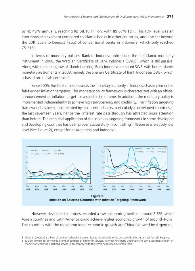
271Transmission Channel and Effectiveness of Dual Monetary Policy In Indonesia
by 45.42% annually, reaching Rp 68.18 Trillion, with 89.67% FDR. This FDR level was an
enormous achievement compared to Islamic banks in other countries, and also far beyondthe LDR (Loan to Deposit Ratio) of conventional banks in Indonesia, which only reached
75.21%.
In terms of monetary policies, Bank of Indonesia introduced the first Islamic monetaryinstrument in 2000, the Wadi»ah Certificate of Bank Indonesia (SWBI)2, which is still passive.
Along with the rapid grow of Islamic banking; Bank Indonesia replaced SWBI with better Islamic
monetary instruments in 2008, namely the Shariah Certificate of Bank Indonesia (SBIS), whichis based on Ju»alah contracts3.
Since 2005, the Bank of Indonesia as the monetary authority in Indonesia has implemented
full-fledged inflation targeting. This monetary policy framework is characterized with an official
announcement of inflation target for a specific timeframe. In addition, the monetary policy isimplemented independently to achieve high transparency and credibility. The inflation targeting
framework has been implemented by most central banks, particularly in developed countries in
the last seventeen years, hence the interest rate pass through has attracted more attentionthan before. The empirical application of the inflation targeting framework in some developed
and developing countries has been proven successfully in controlling inflation at a relatively low
level (See Figure 2), except for in Argentina and Indonesia.
Figure 2.Inflation on Selected Countries with Inflation Targeting Framework
However, developed countries recorded a low economic growth of around 2-3%, while
Asean countries and Latin America could achieve higher economic growth of around 4-6%.
The countries with the most prominent economic growth are China followed by Argentina.
18
15
12
9
6
3
0
-3
JPNGER
UKCAN
RRCS. KOR
2003Mar
2004Mar
2005Mar
2006Mar
2007Mar
2008Mar
2009Mar
2010Mar
18
15
12
9
6
3
0
-3
INAMAL
THAPHIL
ARGBRA
2003Mar
2004Mar
2005Mar
2006Mar
2007Mar
2008Mar
2009Mar
2010Mar
2 Wadi»ah (deposit) is a kind of contract whereby a person leaves his valuable in the custody of others as a trust for safe keeping.3 Ju»alah (reward for service) is a kind of contract of hiring for services, in which one party undertakes to pay a specified amount of
money for rendering a defined service in accordance with the terms negotiated between them.
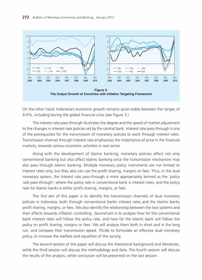
272 Bulletin of Monetary Economics and Banking, January 2012
On the other hand, Indonesia»s economic growth remains quite stable between the ranges of
4-6%, including»during the global financial crisis (see Figure 3.)
The interest rate pass-through illustrates the degree and the speed of market adjustment
to the changes in interest rate policies set by the central bank. Interest rate pass-through is oneof the prerequisites for the transmission of monetary policies to work through interest rates.
Transmission channel through interest rate emphasizes the importance of price in the financialmarkets, towards various economic activities in real sector.
Along with the development of Islamic banking, monetary policies affect not only
conventional banking but also affect Islamic banking since the transmission mechanism may
also pass through Islamic banking. Multiple monetary policy instruments are not limited tointerest rates only, but they also can use the profit sharing, margins or fees. Thus, in the dual
monetary system, the interest rate pass-through is more appropriately termed as the «policyrate pass-through», where the policy rate in conventional bank is interest rates, and the policyrate for Islamic banks is either profit sharing, margins, or fees.
The first aim of this paper is to identify the transmission channels of dual monetary
policies in Indonesia, both through conventional banks interest rates and the Islamic banksprofit sharing, margins, or fees. We also identify the relationship between the two systems and
their effects towards inflation controlling. Second aim is to analyze how far the conventional
bank interest rates will follow the policy rate, and how far the Islamic bank will follow thepolicy on profit sharing, margins or fees. We will analyze them both in short and in the long
run, and compare their transmission speed. Thirdis to formulate an effective dual monetary
policy, to increase the welfare and equalities of the society.
The second session of this paper will discuss the theoretical background and literatures,while the third session will discuss the methodology and data. The fourth session will discuss
the results of the analysis, while conclusion will be presented on the last session.
Figure 3.The Output Growth of Countries with Inflation Targeting Framework
JPNGER
UKCAN
RRCS. KOR
2003Mar
2004Mar
2005Mar
2006Mar
2007Mar
2008Mar
2009Mar
2010Mar
12
9
6
3
0
-3
-6
-9
2003Mar
2004Mar
2005Mar
2006Mar
2007Mar
2008Mar
2009Mar
2010Mar
12
9
6
3
0
-3
-6
-9
INAMAL
THAPHIL
ARGBRA
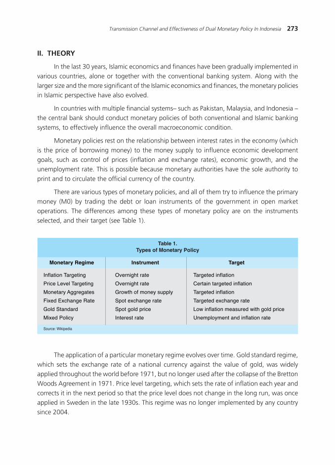
273Transmission Channel and Effectiveness of Dual Monetary Policy In Indonesia
II. THEORY
In the last 30 years, Islamic economics and finances have been gradually implemented in
various countries, alone or together with the conventional banking system. Along with the
larger size and the more significant of the Islamic economics and finances, the monetary policiesin Islamic perspective have also evolved.
In countries with multiple financial systems√ such as Pakistan, Malaysia, and Indonesia √
the central bank should conduct monetary policies of both conventional and Islamic banking
systems, to effectively influence the overall macroeconomic condition.
Monetary policies rest on the relationship between interest rates in the economy (which
is the price of borrowing money) to the money supply to influence economic development
goals, such as control of prices (inflation and exchange rates), economic growth, and theunemployment rate. This is possible because monetary authorities have the sole authority to
print and to circulate the official currency of the country.
There are various types of monetary policies, and all of them try to influence the primary
money (M0) by trading the debt or loan instruments of the government in open marketoperations. The differences among these types of monetary policy are on the instruments
selected, and their target (see Table 1).
Table 1.Types of Monetary Policy
Monetary Regime Instrument Target
Inflation Targeting Overnight rate Targeted inflation
Price Level Targeting Overnight rate Certain targeted inflation
Monetary Aggregates Growth of money supply Targeted inflation
Fixed Exchange Rate Spot exchange rate Targeted exchange rate
Gold Standard Spot gold price Low inflation measured with gold price
Mixed Policy Interest rate Unemployment and inflation rate
Source: Wikipedia
The application of a particular monetary regime evolves over time. Gold standard regime,
which sets the exchange rate of a national currency against the value of gold, was widelyapplied throughout the world before 1971, but no longer used after the collapse of the Bretton
Woods Agreement in 1971. Price level targeting, which sets the rate of inflation each year and
corrects it in the next period so that the price level does not change in the long run, was onceapplied in Sweden in the late 1930s. This regime was no longer implemented by any country
since 2004.
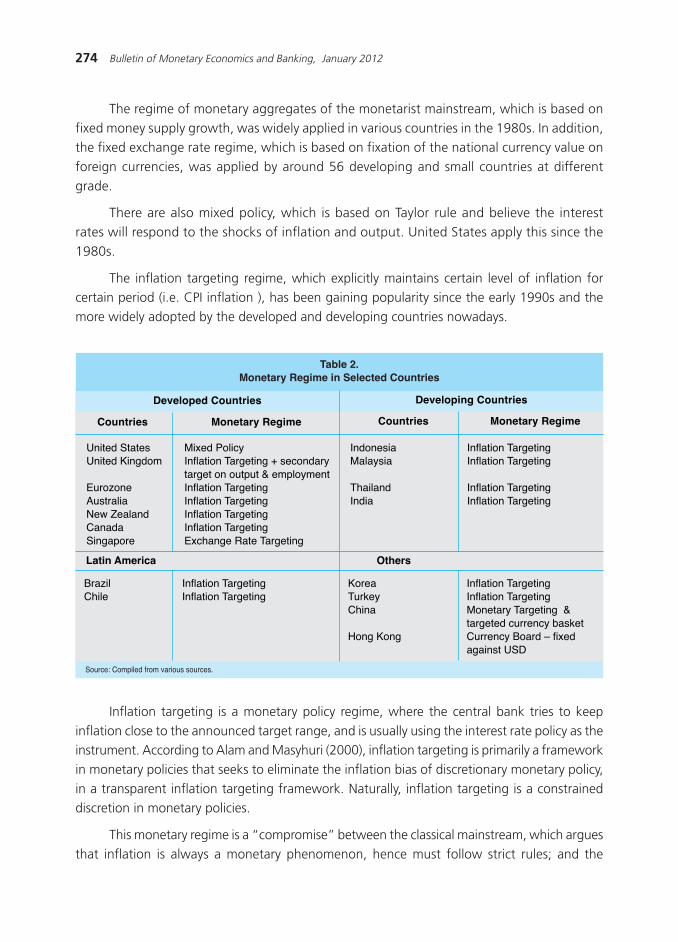
274 Bulletin of Monetary Economics and Banking, January 2012
The regime of monetary aggregates of the monetarist mainstream, which is based on
fixed money supply growth, was widely applied in various countries in the 1980s. In addition,the fixed exchange rate regime, which is based on fixation of the national currency value on
foreign currencies, was applied by around 56 developing and small countries at different
grade.
There are also mixed policy, which is based on Taylor rule and believe the interest
rates will respond to the shocks of inflation and output. United States apply this since the
1980s.
The inflation targeting regime, which explicitly maintains certain level of inflation forcertain period (i.e. CPI inflation ), has been gaining popularity since the early 1990s and the
more widely adopted by the developed and developing countries nowadays.
Inflation targeting is a monetary policy regime, where the central bank tries to keep
inflation close to the announced target range, and is usually using the interest rate policy as theinstrument. According to Alam and Masyhuri (2000), inflation targeting is primarily a framework
in monetary policies that seeks to eliminate the inflation bias of discretionary monetary policy,
in a transparent inflation targeting framework. Naturally, inflation targeting is a constraineddiscretion in monetary policies.
This monetary regime is a ≈compromiseΔ between the classical mainstream, which argues
that inflation is always a monetary phenomenon, hence must follow strict rules; and the
Table 2.Monetary Regime in Selected Countries
Countries Monetary Regime
United States Mixed Policy Indonesia Inflation TargetingUnited Kingdom Inflation Targeting + secondary Malaysia Inflation Targeting
target on output & employmentEurozone Inflation Targeting Thailand Inflation TargetingAustralia Inflation Targeting India Inflation TargetingNew Zealand Inflation TargetingCanada Inflation TargetingSingapore Exchange Rate Targeting
Source: Compiled from various sources.
Developed Countries
Countries Monetary Regime
Developing Countries
Brazil Inflation Targeting Korea Inflation TargetingChile Inflation Targeting Turkey Inflation Targeting
China Monetary Targeting &targeted currency basket
Hong Kong Currency Board – fixedagainst USD
Latin America Others

275Transmission Channel and Effectiveness of Dual Monetary Policy In Indonesia
Keynesians mainstream, which argues that inflation is not caused by the higher amount of
money than goods, but because of the number of worker seeking for job exceed the availableemployment capacity. With this context, monetary policies are responsible to ensure the
equilibrium between demand and supply of the economy, hence must be conducted wisely
(discretion) in accordance with the current development. The compromise is, in the long runthe monetary policy follow the rules, whereas in the short run the monetary policies may have
discretion.
2.1. Conventional Monetary Policy Transmission
From the conventional perspective, the monetary policy can be transmitted through interestrate channel, credit line, exchange rate, asset prices, and expectations channel. The use of
interest rate instruments in inflation targeting, put the interest through pass-through as important
topic.
Models for interest rate pass-through have been developed for a long time. The modeldeveloped by Rousseas (1985), marginal costing pricing model, argue that changes in bank
interest rates will be forwarded in the form of changes in interest rates to their customers
because it reflects the changes of bank»s marginal cost. This model is still considered as the bestmodel to explain the interest rate pass-through from policy rates to bank interest (Egert et al,
2006). The general representation of the model equation is:
(1)
Where br is interest rates set by banks; γ0 is mark-up; and mr is the marginal cost price,
substituted with the market interest rate.
Several factors can explain the spread between the retail rate and the marginal cost offunds, such as the level of competition (the higher the competition the lower the spread), the
difference in interest rates for different customers, and the asymmetric information between
borrowers and lenders. According to Bredin (2002), there are three categories of variable thatmay affect the level and speed of pass-through from policy rates to bank interest rates; monetary
policies, the level of banking competition, and other factors.
On empirical ground, some studies use a standard single equation Error Correction
Model (ECM), for example Mojon (2000), Bredin (2001), de Bondt (2002), Espinosa-Vegaand Rebucci (2003), Chmielewski (2004), Tiemen (2004), Horvath et.al. (2005), Betancourt
et.al. (2008), and van Leuvensteijn et.al. (2008). The estimated equation proposed by de
Bondt (2002) is:
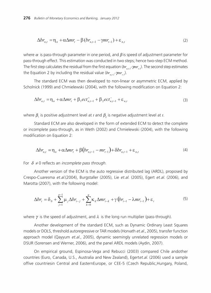
276 Bulletin of Monetary Economics and Banking, January 2012
where α is pass-through parameter in one period, and β is speed of adjustment parameter for
pass-through effect. This estimation was conducted in two steps; hence two-step ECM method.The first step calculates the residual from the first equation (br
n,t-1-γmr
t-1). The second step estimates
the Equation 2 by including the residual value (brn,t-1
-γmrt-1
).
The standard ECM was then developed to non-linear or asymmetric ECM, applied byScholnick (1999) and Chmielewski (2004), with the following modification on Equation 2:
(2)
(3)
where β1 is positive adjustment level at t and β2 is negative adjustment level at t.
Standard ECM are also developed in the form of extended ECM to detect the complete
or incomplete pass-through, as in Weth (2002) and Chmielewski (2004), with the followingmodification on Equation 2:
(4)
For δ = 0 reflects an incomplete pass through.
Another version of the ECM is the auto regressive distributed lag (ARDL), proposed by
Crespo-Cuaresma et.al.(2004), Burgstaller (2005), Lie et.al. (2005), Egert et.al. (2006), and
Marotta (2007), with the following model:
(5)
where γ is the speed of adjustment, and λ is the long run multiplier (pass-through).
Another development of the standard ECM, such as Dynamic Ordinary Least Squaresmodels or DOLS, threshold autoregressive or TAR models (Horvath et.al., 2005), transfer function
approach model (Qayyum et.al., 2005), dynamic seemingly unrelated regression models or
DSUR (Sorensen and Werner, 2006), and the panel ARDL models (Aydin, 2007).
On empirical ground, Espinosa-Vega and Rebucci (2003) compared Chile andothercountries (Euro, Canada, U.S., Australia and New Zealand), Egertet.al. (2006) used a sample
offive countriesin Central and EasternEurope, or CEE-5 (Czech Republic,Hungary, Poland,

277Transmission Channel and Effectiveness of Dual Monetary Policy In Indonesia
Slovakia, and Slovenia), while Sorensen and Werner (2006) used a sample of Euro area countries
with the dynamic data panel and ECM method.
Egert et.al.(2006) foundthat the interest rate pass-through effect in the CEE-5 was low
and decreased along years of observation, due to the absence of co-integration between the
policy rate and the bank interest rates (short and long run), and is expected to continue decliningin the future.
Sorensen and Werner (2006) found a large heterogeneity in the Euro countries
both on the long-run pass-through equilibrium and its speed of adjustment.These results
also confirm the slow and incomplete adjustment process of bank interest rate onpolicyrate.
Horvath et.al. (2005) found corporate lending rates adjusted quickly and completely to
the changes of interest rate policy, while the deposit rates and household loans adjusted slowlyand incompletely. Qayyum et.al. (2005) found the pass-through of policy rate (T-Bills rate) to
the call money rate is complete in a month, while the pass-through from policy rates to deposit
rates and bank loans take longer. Liu et.al. (2005) concluded that there is a complete long runpass-through for some interest rates in New Zealand, and generally, confirmed that the policy
rates have greater influence on short-run interest rates and that an increase in transparency
increases the effectiveness of monetary policy.
Recent studies link the interest rate pass-through to the implementation of Euro (Marotta,
2007), to the macro-economic variables that also affect interest rates (Betancourt et.al., 2008),
to the optimal monetary policy (Kobayashi, 2008), and to the competition among banks (VanLeuvensteijnet.al., 2008).
Marotta (2007) examined the structural breaks in the interest rate pass-through from
policy rates to bank lending rates and the process of unification of the Euro. The result shows
that the EU members have different speeds of adjustment to the Euro unification in the January1999, and they adjusted to the new monetary regime slowly. He also found that the interest
rate pass-through in EU countries are incomplete, which means that the uniform monetary
policy is less effective. These results are contrary to the economic intuition that thed ecline inthe volatility of policy rate (money market rate) will faster the transmission from policy rate to
the bank»s interest rate.
Betancourt (2008) conducted a study on interest rate pass-through in Colombia frommicro banking perspective with monthly data during 1999-2006, using the single equation
error correction model (EC) and the vector autoregressive model (VAR). It is based on the
microeconomic theory that the effect of interest rate policy on banking is acomplex processand also depends on the macroeconomic variables. The result of the two models supports
the hypo thesis that besides interest rate policy, macroeconomic variables also affect the
transmission mechanism of monetary policy to the banking interest rate. In addition, the EC
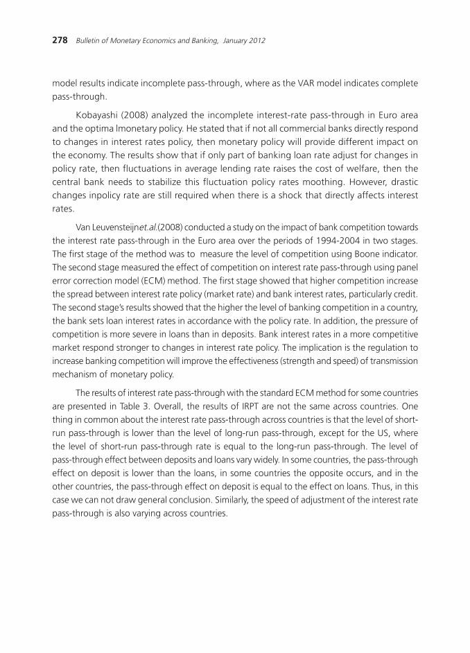
278 Bulletin of Monetary Economics and Banking, January 2012
model results indicate incomplete pass-through, where as the VAR model indicates complete
pass-through.
Kobayashi (2008) analyzed the incomplete interest-rate pass-through in Euro area
and the optima lmonetary policy. He stated that if not all commercial banks directly respond
to changes in interest rates policy, then monetary policy will provide different impact onthe economy. The results show that if only part of banking loan rate adjust for changes in
policy rate, then fluctuations in average lending rate raises the cost of welfare, then the
central bank needs to stabilize this fluctuation policy rates moothing. However, drasticchanges inpolicy rate are still required when there is a shock that directly affects interest
rates.
Van Leuvensteijnet.al.(2008) conducted a study on the impact of bank competition towards
the interest rate pass-through in the Euro area over the periods of 1994-2004 in two stages.The first stage of the method was to measure the level of competition using Boone indicator.
The second stage measured the effect of competition on interest rate pass-through using panel
error correction model (ECM) method. The first stage showed that higher competition increasethe spread between interest rate policy (market rate) and bank interest rates, particularly credit.
The second stage»s results showed that the higher the level of banking competition in a country,
the bank sets loan interest rates in accordance with the policy rate. In addition, the pressure ofcompetition is more severe in loans than in deposits. Bank interest rates in a more competitive
market respond stronger to changes in interest rate policy. The implication is the regulation toincrease banking competition will improve the effectiveness (strength and speed) of transmission
mechanism of monetary policy.
The results of interest rate pass-through with the standard ECM method for some countries
are presented in Table 3. Overall, the results of IRPT are not the same across countries. Onething in common about the interest rate pass-through across countries is that the level of short-
run pass-through is lower than the level of long-run pass-through, except for the US, where
the level of short-run pass-through rate is equal to the long-run pass-through. The level ofpass-through effect between deposits and loans vary widely. In some countries, the pass-through
effect on deposit is lower than the loans, in some countries the opposite occurs, and in the
other countries, the pass-through effect on deposit is equal to the effect on loans. Thus, in thiscase we can not draw general conclusion. Similarly, the speed of adjustment of the interest rate
pass-through is also varying across countries.

279Transmission Channel and Effectiveness of Dual Monetary Policy In Indonesia
Table 3.Interest Rate Pass-Through using Standard ECM on selected Countries
Country
Bredin et al.2001
De Bondt2002
Espinosa-Vega &Rebucci 2003
Chmielewski2004
Tieman 2004
Horvath et al.2005
Note: S is deposit; P is loan; Pdk is short term; Pjg is long term. The highlighted cell represents complete pass-through condition.
0.35-0.98
0.39-0.68
0.60-0.72
0.93-0.98
0.64-1.00
0.67-0.81
0.71-0.74
0.75-0.88
0.80 0.49
0.82 0.90
0.98 0.91
..… -0.78
1.00 1.27
1.41 1.57
0.86 0.87
AuthorShort Term
Deposit Loan
Long Term
Deposit LoanAdjustment Notes
Ireland
Euro area
Chile
Euro
Canada
US
Australia
NewZealand
Polandia
Czech
Hungary
Polandia
Romania
Slovak
Slovenia
Hungary
0.32-0.35
0.20-0.68
0.27-0.57
1.05-1.13
0.84-1.00
0.40-0.87
0.34-0.42
0.22-0.57
0.09 -0.02
0.22 0.07
0.29 0.23
..… -0.30
0.04 0.23
0.16 0.11
0.41 0.64
0.13-0.54
0.18-0.63
0.18-0.43
0.46-0.83
0.86
0.46
0.21
0.47-0.68
0.07 0.19
-0.15 0.01
0.18 0.10
-0.46 -044.
-0.02 0.07
0.16 0.15
0.05 0.67
Str Break
S≈P S<PPdk < Pjg
S≈P S<PPdk < Pjg
S>P S>PPdk < Pjg
S>P S>PPdk ≈ Pjg
S≈P S<PPdk ≈ Pjg
S≈P S<PPdk < Pjg
S>P S≈PPdk < Pjg
S<P S<PPdk < Pjg
S≈P S≈PPdk < Pjg
S≠P S≈PPdk < Pjg
S>P S≈PPdk < Pjg
S≈P S≈PPdk < Pjg
S>P S≈PPdk < Pjg
S≈P S≈PPdk < Pjg
S≈P S≈PPdk < Pjg
0.64-0.88
0.92-1.53
0.55-0.88
0.57-0.82
0.24-1.01
1.00
1.09
0.77
0.85-1.02
0.76 0.65
1.10 0.67
0.85 0.96
0.80 0.73
1.62 0.79
2.08 1.85
0.81 0.98
0.25-0.72
S 3-15 monthP 3-10 month
S 1/2-4 monthP 2/3-2 month
S 1 1/2-17 monthP 3-11 month
S ≈0 monthP _-4 month
S 0-2 monthP 0.2 month
S _-1.4 monthP 3.86 month
S 2-2_ monthP 2 month
S 1-4 monthP 1_-5 month
S 1_ 8.1 monthP 2.4 4.4 month
S 1.6 2.8 monthP 10_ 9_ month
S 36.8 2 monthP 6.4 10 month
S ..… 5_ monthP 3_ 4 month
S 6.9 22_ monthP 9_ 5.8 month
S 5_ 6_ monthP 11.2 9_ month
S 3 – 2 monthP 4 – 2 month

280 Bulletin of Monetary Economics and Banking, January 2012
Table 4 gives the variation of the level of pass-through on deposit and loans across
countries. However, in general there isa certain pattern. In the short run, the pass-throughdeposit is equal to or greater than the pass-through loans. In the long run, the pass-through
deposit is equal to or smaller than the pass-through loans. Most empirical studies show that
the level of pass-through deposit equal to the level of pass-through loans in the short andlong run.
Table 4. Interest Rate Pass-Through using Standard ECM on Selected Countries
Deposit < Loan Deposit ≈ Loan Deposit > Loan
Chile (Pjg)
Euro area (Pjg)
US (Pjg)
Australia (Pjg)
Polandia (Pdk, Pjg)
Chile (Pdk)
Euro area (Pdk)
US (Pdk)
Australia (Pdk)
New Zealand (Pjg)
Czech (Pdk, Pjg)
Polandia (Pjg)
Romania (Pdk, Pjg)
Slovak (Pjg)
Hungary (Pdk, Pjg)
Slovenia (Pdk, Pjg)
Euro (Pdk, Pjg)
Canada (Pdk, Pjg)
New Zealand (Pdk)
Polandia (Pdk)
Slovak (Pdk)
2.2. Islamic Monetary Transmission Policy
Transmission of monetary policye merged since the separation of the monetary authority
from fiscal authorities. Monetary authorities evolved in line with the development of central
bank from circulation bank (issuing paper money or fiat money), which marked by theestablishment of Bank of England (BOE) in 1694 (Capie, 1994). Because of its inflationary
paper money (since it has no intrinsic value) then the task of central bank increased, including
setting the money supply to control the value of currency or inflation. This is not necessarywhen the money has intrinsic value, like the gold Dinar and silver Dirham during Islamic
caliphate. The last Khilafah Islamiyah, the Ottoman dynasty in Turkey, collapsed in 1924
(Islahi, 2004).
In conventional economic domination with its central bank and fiat money, Islamiceconomics grow in Muslim-majority countries within the system of paper money and central
banks. Therefore, Islamic monetary system with its policies and transmission processes also
grew. A pioneer of the theory of contemporary Islamic monetary economics is MuhammadUmer Chapra in his book ΔTowards a Just Monetary System (1985)Δ.
281Transmission Channel and Effectiveness of Dual Monetary Policy In Indonesia
The setting of contemporary Islamic financial institutions are not much different from
the setting of conventional financial institutions, hence the Islamic monetary policy instrumentsare also similar with the instruments of the conventional one. Since both systems have similar
and also different instruments, the Islamic monetary policy transmission can be similar or different
from the conventional one. Chapra (1985) did not discuss specifically the issue of Islamic monetarypolicy transmission. Further development of Islamic monetary theory also does not mention it;
including pass-through or its channels (see Siddiqui, 2007).
However, few empirical studies a rise to see the Islamic monetary policy transmissioncharacteristics. Sukmana and Kassim(2010) was an initial attempt to determine the transmission
of monetary policy through financing channel to economic growthin Malaysian Islamic banking
system, which is simply defined as follows:
(6)
Where IP is industrial production index, IF is Islamic financing, ID is third party fund collectedin Islamic bank, and ONIGHT is overnight interbank interest rate, representing the monetary
policy.
The same framework has been carried out by Ascarya (2010) for the case of Indonesia inorder to determine the transmission of monetary policy to the ultimate goal of monetary policy
(namely economic growt hand stability of the money), via financing channel in Islamic banking.
The model is simply defined as follows:
(7)
(8)
Where IPI is industrial production index, CPI is consumer price index, IFIN is Islamic bankfinancing, IDEP is third party financing or funds in Islamic bank and PUAS is interest rate of
Islamic interbank money market.
In addition, Ayuniyyah, et.al.(2010) examined the multiple transmission of monetary policyin Indonesia in order to grow the economic. The model is simply formulated as:
and
(9)
282 Bulletin of Monetary Economics and Banking, January 2012
(10)
(11)
Where ibr is funding or financing yield set by Islamic banks, γ0 is mark-upand imr is the marginal
cost price, substituted with market return.
For equation to estimate, we refer Bde Bondt (2002), with the following
modification:
where IPI is industrial production index, nIFIN is total Islamic bank financing, nCCRD is total
conventional bank credit, nIDEP is financing or funds from an Islamic third part, nCDEP istotal financing or funds from a conventional bank, iIDEP is Islamic banking deposits yield,
iCDEP is conventional banking deposits yield, SBIS is the yields of Syariah Certificates of Bank of
Indonesia, and SBI is the yields of Certificates of Bank Indonesia.
The conventional interest rate pass-through model (Egerti, 2006) was modified to formulate
the Islamic pass-through rate policy model. Equation (1) is modified as follows:
Where α is pass-through parameter for one period, and β is the speed of pass-throughadjustment.
The first step is to calculate the residual of Equation 10 (ibrn,t-1
-γimrt-1
). The second step is
use the residual (ibrn,t-1
-γimrt-1
), then estimate Equation 11.
III. METHODOLOGY
This paper uses quantitative approach to analyze monetary policy in a dual financial
system; conventional and Islamic. Empirical model that is built refers to the conceptual frameworkas illustrated in Figure 4.
Dual monetary policy in Indonesia used multiple monetary policy instruments, namely
Certificate of Bank of Indonesia or SBI-based interest rates for conventional system, and Islamic
SBI or SBIS-based fee for Islamic banking, which are still referring to the SBI rate. SBI interestrate and SBIS fee are policy rates.Policy rates will affect the funding and the bank financing
through the interbank money market both in conventional and Islamic banking, then will affect
the costof fund channeling. Expansion of credit and financing will finally affect the level ofoutput and inflation.
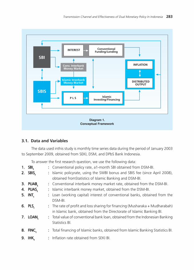
283Transmission Channel and Effectiveness of Dual Monetary Policy In Indonesia
Diagram 1.Conceptual Framework
INFLATION
INTEREST
SBI
SBIS
DISTRIBUTEDOUTPUT
P L S
ConventionalFunding/Lending
IslamicInvesting/Financing
Conv. InterbankMoney Market
Islamic InterbankMoney Market
3.1. Data and Variables
The data used inthis study is monthly time series data during the period of January 2003
to September 2009, obtained from SEKI, DSM, and DPbS Bank Indonesia.
To answer the first research question, we use the following data:
1.1.1.1.1. SBISBISBISBISBIttttt ::::: Conventional policy rate, a1-month SBI obtained from DSM-BI.
2.2.2.2.2. SBISSBISSBISSBISSBISttttt ::::: Islamic policyrate, using the SWBI bonus and SBIS fee (since April 2008),
obtained fromStatistics of Islamic Banking and DSM-BI.
3.3.3.3.3. PUABPUABPUABPUABPUABttttt ::::: Conventional interbank money market rate, obtained from the DSM-BI.
4.4.4.4.4. PUASPUASPUASPUASPUASttttt ::::: Islamic interbank money market, obtained from the DSM-BI.
5.5.5.5.5. INTINTINTINTINTttttt ::::: Loan (working capital) interest of conventional banks, obtained from the
DSM-BI.
6.6.6.6.6. PLSPLSPLSPLSPLSttttt ::::: The rate of profit and loss sharing for financing (Musharaka + Mudharabah)
in Islamic bank, obtained from the Directorate of Islamic Banking BI.
7.7.7.7.7. LOANLOANLOANLOANLOANttttt ::::: Total value of conventional bank loan, obtained from the Indonesian Banking
Statistics BI.
8.8.8.8.8. FINCFINCFINCFINCFINCttttt ::::: Total financing of Islamic banks, obtained from Islamic Banking Statistics BI.
9.9.9.9.9. IHKIHKIHKIHKIHKttttt ::::: Inflation rate obtained from SEKI BI.

284 Bulletin of Monetary Economics and Banking, January 2012
Diagram 2.Dual Monetary Transmission Channel (Conventional and Syariah)
SBI
INF/GD
PUAB
SBIS PUAS
INT
PLS
LOAN
FIN
(12)
(13)
3.2. Estimation Techniques
This study will use several estimation techniques, namely Granger Causality and Vector
Auto regression (VAR)/Vector Error Correction Model (VECM), Standard Error Correction Model
with two-steps, and descriptive analysis.
To answer the first research question (identify the dual monetary policy transmissionchannel in Indonesia, both through the conventional and Islamic system, and also their link),
we use the Granger Causality technique. Causality relationships among the variables are based
on the following conceptual framework:
To answer the second research question, we canuse the Vector AutoRegression (VAR). In
the presence of cointegration, we will usethe Vector Error Correction Model (VECM).
VAR is a system of n equation, with n endogenous variables. Each endogenous variableisexplained by its own lag, current value of other endogenous variable, and the lag of other
endogenous variables. Therefore, in the context of modern econometrics, VAR is considered as
a multivariate time-series that treat all variable endogenously since there is nocertainty if thevariable is actually exogenous, and is fully rely on the data to explain. Sims (1980) argues that
if there is a true simultaneity among a number of variables, then the variables must be treated
equally and there should be no a priori distinction between endogenous and exogenous variables.Enders (2004) formulated the simple first-order bivariate system as follows:
285Transmission Channel and Effectiveness of Dual Monetary Policy In Indonesia
Assuming that yt and z
t is stationary, ε
yt and ε
zt are white noise disturbances with standard
deviation σy and σ
z ; while εyt and ε
zt are white noise and uncorrelated disturbance. Meanwhile,we can write the standard form of the primitive model above as follows.
(14)
(15)
eyt and e
zt are the combination of ε
yt and ε
zt . The primitive form is called the structural VAR, and
the standard form is called VAR. Detail explanation on transforming the primitive to standardforms is available in Enders(2004). The general VAR model can be presented as:
(16)
xt is the (n x 1) vector of endogenous variable; μ
t is the vector of exogenous variable, including
intercept andtrend; Ai is (n x n) coefficientmatrix ; and εt is the residual vector. In a simplebivariate system of y
t and z
t , the variable y
t is influenced by the present and past value of z
t,
while zt is influenced by the present and the past value of y
t .
To overcome the shortcoming of first-differenced VAR and to regain long-run relationshipsbetween variables, we can use Vector Error Correction Model (VECM), as long as these variables
are co-integrated. Inserting the original equation in level into the new equations, we have :
(17)
(18)
a is the long-runcoefficient, b is the short run coefficient, λ is the error correction parameter,
and the term in parentheses indicate co-integration between variables y and z.
General VECM model scan be presented as follows (Achsani etal, 2005):
(19)
Π and Γ is the function ofAi . The matrixΩΠ can be decomposed into two matrices with
dimensions (n x r); ΩΠ = λβT , where λ is the adjustment matrix and β is the co-integrationvector, whereas r is the co-integration rank.
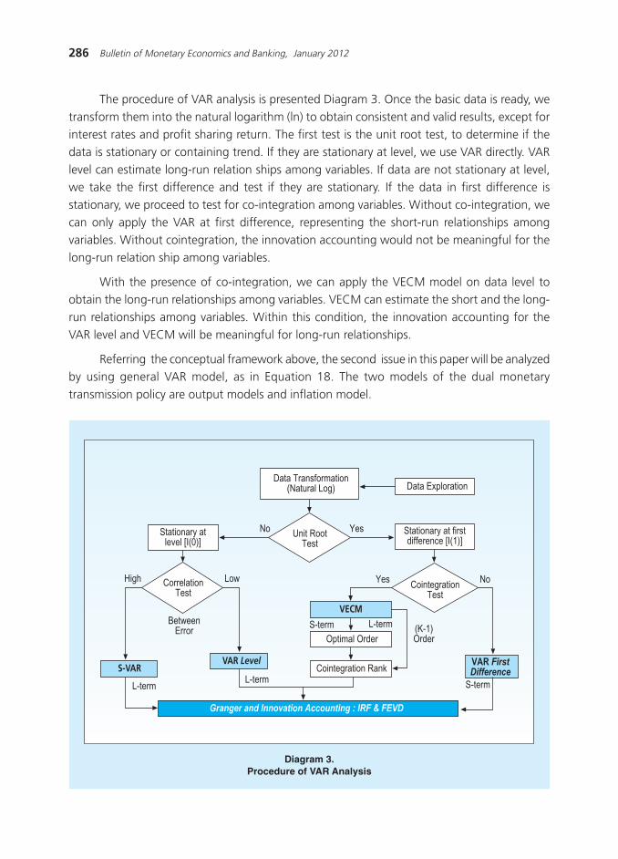
286 Bulletin of Monetary Economics and Banking, January 2012
Diagram 3.Procedure of VAR Analysis
Data Transformation(Natural Log)
Unit RootTest
Stationary atlevel [I(0)]
Stationary at firstdifference [I(1)]
CointegrationTest
VECM
VAR FirstDifference
Optimal Order
Cointegration Rank
Granger and Innovation Accounting : IRF & FEVD
Data Exploration
(K-1)Order
YesNo
Yes No
S-term
S-termL-term
L-term
CorrelationTest
VAR LevelS-VAR
High Low
BetweenError
L-term
The procedure of VAR analysis is presented Diagram 3. Once the basic data is ready, we
transform them into the natural logarithm (ln) to obtain consistent and valid results, except forinterest rates and profit sharing return. The first test is the unit root test, to determine if the
data is stationary or containing trend. If they are stationary at level, we use VAR directly. VAR
level can estimate long-run relation ships among variables. If data are not stationary at level,we take the first difference and test if they are stationary. If the data in first difference is
stationary, we proceed to test for co-integration among variables. Without co-integration, we
can only apply the VAR at first difference, representing the short-run relationships amongvariables. Without cointegration, the innovation accounting would not be meaningful for the
long-run relation ship among variables.
With the presence of co-integration, we can apply the VECM model on data level toobtain the long-run relationships among variables. VECM can estimate the short and the long-
run relationships among variables. Within this condition, the innovation accounting for the
VAR level and VECM will be meaningful for long-run relationships.
Referring the conceptual framework above, the second issue in this paper will be analyzedby using general VAR model, as in Equation 18. The two models of the dual monetary
transmission policy are output models and inflation model.
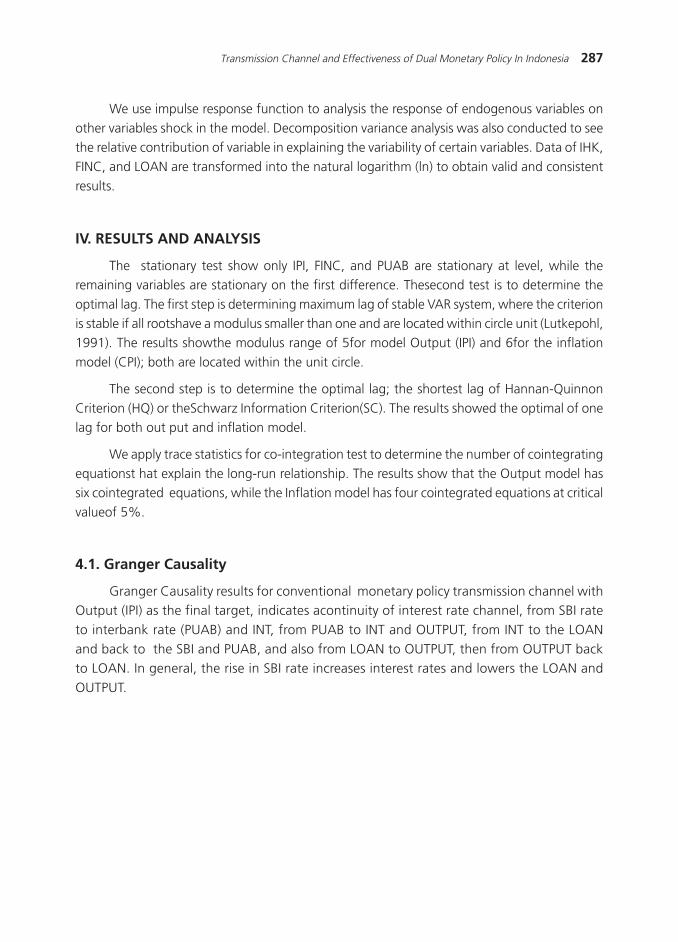
287Transmission Channel and Effectiveness of Dual Monetary Policy In Indonesia
We use impulse response function to analysis the response of endogenous variables on
other variables shock in the model. Decomposition variance analysis was also conducted to seethe relative contribution of variable in explaining the variability of certain variables. Data of IHK,
FINC, and LOAN are transformed into the natural logarithm (ln) to obtain valid and consistent
results.
IV. RESULTS AND ANALYSIS
The stationary test show only IPI, FINC, and PUAB are stationary at level, while theremaining variables are stationary on the first difference. Thesecond test is to determine the
optimal lag. The first step is determining maximum lag of stable VAR system, where the criterion
is stable if all rootshave a modulus smaller than one and are located within circle unit (Lutkepohl,1991). The results showthe modulus range of 5for model Output (IPI) and 6for the inflation
model (CPI); both are located within the unit circle.
The second step is to determine the optimal lag; the shortest lag of Hannan-Quinnon
Criterion (HQ) or theSchwarz Information Criterion(SC). The results showed the optimal of onelag for both out put and inflation model.
We apply trace statistics for co-integration test to determine the number of cointegrating
equationst hat explain the long-run relationship. The results show that the Output model hassix cointegrated equations, while the Inflation model has four cointegrated equations at critical
valueof 5%.
4.1. Granger Causality
Granger Causality results for conventional monetary policy transmission channel withOutput (IPI) as the final target, indicates acontinuity of interest rate channel, from SBI rate
to interbank rate (PUAB) and INT, from PUAB to INT and OUTPUT, from INT to the LOAN
and back to the SBI and PUAB, and also from LOAN to OUTPUT, then from OUTPUT backto LOAN. In general, the rise in SBI rate increases interest rates and lowers the LOAN and
OUTPUT.
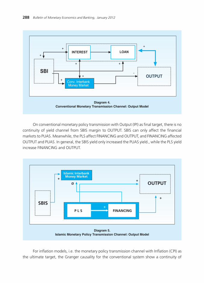
288 Bulletin of Monetary Economics and Banking, January 2012
On conventional monetary policy transmission with Output (IPI) as final target, there is nocontinuity of yield channel from SBIS margin to OUTPUT. SBIS can only affect the financial
markets to PUAS. Meanwhile, the PLS affect FINANCING and OUTPUT, and FINANCING affected
OUTPUT and PUAS. In general, the SBIS yield only increased the PUAS yield., while the PLS yieldincrease FINANCING and OUTPUT.
Diagram 4.Conventional Monetary Transmission Channel: Output Model
OUTPUT
Conv. InterbankMoney Market
INTEREST
SBI
LOAN+
+
+
+
+
+
-
+
OUTPUT
SBIS
Islamic InterbankMoney Market
P L S FINANCING
+
+
+
+
Diagram 5.Islamic Monetary Policy Transmission Channel: Output Model
For inflation models, i.e. the monetary policy transmission channel with Inflation (CPI) as
the ultimate target, the Granger causality for the conventional system show a continuity of

289Transmission Channel and Effectiveness of Dual Monetary Policy In Indonesia
interest rate from SBI to PUAB and INT, from PUAB to INT, from INT to LOAN and INFLATION
and back again to SBI and PUAB. After that, INFLATION affected SBI. In general the rise in SBincreases interest rate, lowers the LOAN and increase INFLATION.
Diagram 6.Conventional Monetary Policy Transmission Channel: Inflation Model
Conv. InterbankMoney Market
INTEREST
SBI
LOAN
+
+
+
-
+
+
+
+
+
-
INFLATION
On the other hand, for the Islamic monetary policy transmission in Inflation model (CPI),
the Granger Causality indicated the discontinuity continuous from SBIS yield to inflation. SBISonly affects the yield of PUAS Islamic financial market. Meanwhile, PLS affect FINANCING then
FINANCING affects PUAS. In contrast, PUAS, PLS and FINANCING were affected by INFLATION.
Diagram 7.Islamic Monetary Policy Transmission Channel: Inflation Model
INFLATION
SBIS
Islamic Interbank
Money Market
P L S FINANCING
-
Ø
+
+Ø
Ø
290 Bulletin of Monetary Economics and Banking, January 2012
In general, the increase of SBIS yield only increase the PUAS yield, while INFLATION lowered
the PLS and increase FINANCING.
From the Granger test results above, the conventional monetary policy transmission channel
is continuous to OUTPUT, especiallyloan, because conventional loans are parts of the real sector
activities. On the other hand, in Islamic monetary policy transmission channel, the financialsector (SBIS and PUAS) are separated from thereal sector (PLS and FINANCING), and only real
sector link to OUTPUT. Worth to note, in conventional side, the increase of SBI reduces the
output, since funds are absorbed into the financial sector rather than to the real sector.
In inflation models, the channel of conventional monetary policy transmission is continuousto inflation, while Islamic channel is not. This is possible since the conventional interest-based
economy has two dichotomous markets (financial and real sector markets), where the financial
market is inflationary. On the other hand, the Islamic one is non-interest-based and focuses onreal sector, hence non-inflationary. Therefore, the interest rate (representing the price in the
conventional financial sector) affects inflation, while the SBIS (not representing the price in real
sector and financial sector) does not affect inflation. When the Islamic system still use SWBIwith wadiah akad, the SBIS represent the price in Islamic real sector, and when it use SBIS with
ju»alah akad, (profit sharing, which is comparable tothe one-month SBI), SBIS more represent
the price of conventional financial sector.
The conventional system affect the Islamic system mainly on loan, since the monetary
and financial system in Indonesia is still dominated (97.4%) by conventional systems, and the
real sector is related to credit, not the interest rates. On the other hand, Islamic sides affect theconventional side more from the financing yields (PLS), since it is basically a real sector. Meanwhile,
conventional loan interest rates (INT) did not affect the Islamic side since INT is the price of
money in the financial sector, which is depends on many variables.
Generally, conventional monetary policy transmission is in line with the theory, while the
transmission channel of Islamic monetary policy cannot be clearly identified. However, Islamic
instruments using profit and loss sharing, such as mudharabah and musharakah in PLS financing,positively affect the OUTPUT and inflation .
4.2. Impulse Response Function
The results of Impulse Response Function (IRF) for the dual monetary policy transmissionoutput models show that all conventional variables, namely credit (LOAN), interest (INT), interbank
money market (Interbank) and the policy rate (SBI), permanently lower the output. On the
other hand, all the variables of the Islamic Policy Rate, namely financing (FINC), profit sharing(PLS), Islamic interbank money market (PUAS) and Islamic Policy Rate (SBIS), have positive
impact in terms of increasing output permanently.
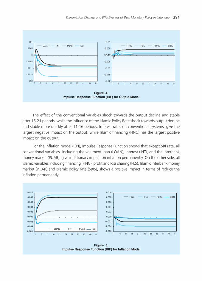
291Transmission Channel and Effectiveness of Dual Monetary Policy In Indonesia
The effect of the conventional variables shock towards the output decline and stableafter 16-21 periods, while the influence of the Islamic Policy Rate shock towards output decline
and stable more quickly after 11-16 periods. Interest rates on conventional systems give the
largest negative impact on the output, while Islamic financing (FINC) has the largest positiveimpact on the output.
For the inflation model (CPI), Impulse Response Function shows that except SBI rate, all
conventional variables including the volumeof loan (LOAN), interest (INT), and the interbankmoney market (PUAB), give inflationary impact on inflation permanently. On the other side, all
Islamic variables including financing (FINC), profit and loss sharing (PLS), Islamic interbank money
market (PUAB) and Islamic policy rate (SBIS), shows a positive impact in terms of reduce theinflation permanently.
FINC PLS PUAS SBIS
-0.02
-0.015
-0.01
-0.005
3E-17
0.005
0.01
1 6 11 16 21 26 31 36 41 46 51
LOAN INT PUAB SBI
1 6 11 16 21 26 31 36 41 46 51- 0.02
- 0.015
- 0.01
- 0.005
0
0.005
0.01
Figure 4.Impulse Response Function (IRF) for Output Model
- 0.006
- 0.004
- 0.002
0.000
0.002
0.004
0.006
0.008
0.010
1 6 11 16 21 26 31 36 41 46 51
FINC PLS PUAS SBIS
-0.006
-0.004
-0.002
0.000
0.002
0.004
0.006
0.008
0.010
1 6 11 16 21 26 31 36 41 46 51
LOAN INT PUAB SBI
Figure 5.Impulse Response Function (IRF) for Inflation Model

292 Bulletin of Monetary Economics and Banking, January 2012
The effect of conventional variables shock to inflation decline and stable after 8-21
period, while the influence of Islamic variables shock on inflation decline slightly faster andstable after 9-19 periods. Among conventional variables, the loan interest rate (INT) have the
largest negative impact (triggering) on inflation, while the Islamic profit and loss sharing (PLS)
have the largest positive impact (reduce) on inflation.
The same result applies for conventional loans (LOAN) and Islamic financing (FINC). Since
the credit is influenced by its interest rates, while the financing is affected by its profit sharing,
then the loan has a negative impact on inflation and output, while Islamic financing had apositive impact on inflation and output. This pattern also applies for the conventional interbank
rate (PUAB) and Islamic interbank yield (PUAS). Since PUAB rate as the reference of conventional
banking interest rate give negative impact on inflation and output. On the other hand PUASpositively affect to the inflation and output.
Furthermore,the Islamic monetary policy(SBIS) also showed similar behavior with other
Islamic variables; reducing inflation and encouraging the output.
Meanwhile, the effects of shock (increase) in SBI may affect (retain) inflation, but at thesame time, it also have a negative impact on output. SBI influence on inflation is the premise of
conventional economics to use the SBI as the main monetary instrument in controlling inflation.
However, it should be noted that the negative influence of the other three conventiona l variables(PUAB, and LOAN INTEREST) is much larger than the positive effect of SBI on inflation.
The impact of interest rates and inflation are in accordance with the results of empirical
studies by Ascarya (2009a and 2009b), where the interest rate is one of the causes of inflation,while profit sharing does not trigger the inflation. The impact of the interest rate and profit
sharing towards output was in accordance with Ryandono (2006) and Ascarya et.al. (2007),
where the interest rates gave negative impact to output or economic growth, while the profitsharing gave a positive impact to output or economic growth. When the interest rate increased,
investment would decrease, so that the output would decrease as well. Meanwhile, when the
profit sharing increased, the investment would increase, so that the output would increase aswell.
4.3. Forecast Error Variance Decomposition
For the model of dual monetary policy transmission channel with the final output (IPI) asthe target, the Forecast Error Variance Decomposition (FEVD) indicates that the conventional
variables with largest negative contribution (inhibitory) on output includes the interest rate
(18:13%), SBI(5:02% ), Interbank (4:57%) and LOAN(3:57%). On the other hand, the Islamicvariable sturned out to be apositive contributor on driving the output, though still small, like
the FINC (1.12%) and PLS (0.36%).
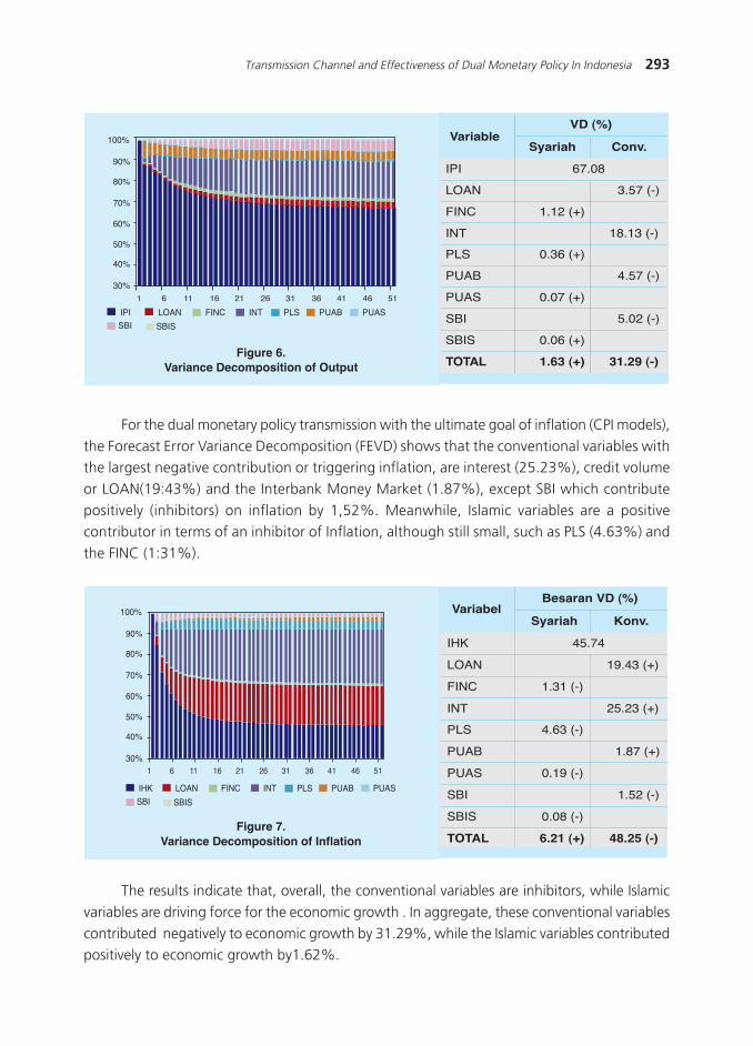
293Transmission Channel and Effectiveness of Dual Monetary Policy In Indonesia
For the dual monetary policy transmission with the ultimate goal of inflation (CPI models),
the Forecast Error Variance Decomposition (FEVD) shows that the conventional variables withthe largest negative contribution or triggering inflation, are interest (25.23%), credit volume
or LOAN(19:43%) and the Interbank Money Market (1.87%), except SBI which contribute
positively (inhibitors) on inflation by 1,52%. Meanwhile, Islamic variables are a positivecontributor in terms of an inhibitor of Inflation, although still small, such as PLS (4.63%) and
the FINC (1:31%).
Figure 6.Variance Decomposition of Output
Syariah Conv.
IPI
LOAN 3.57 (-)
FINC 1.12 (+)
INT 18.13 (-)
PLS 0.36 (+)
PUAB 4.57 (-)
PUAS 0.07 (+)
SBI 5.02 (-)
SBIS 0.06 (+)
TOTAL 1.63 (+) 31.29 (-)
VariableVD (%)
67.08
1 6 11 16 21 26 31 36 41 46 51
30%
40%
50%
60%
70%
80%
90%
100%
INTIPI LOAN FINC PLS PUAB PUAS
SBI SBIS
Figure 7.Variance Decomposition of Inflation
Syariah Konv.
IHK
LOAN 19.43 (+)
FINC 1.31 (-)
INT 25.23 (+)
PLS 4.63 (-)
PUAB 1.87 (+)
PUAS 0.19 (-)
SBI 1.52 (-)
SBIS 0.08 (-)
TOTAL 6.21 (+) 48.25 (-)
VariabelBesaran VD (%)
45.74
30%
40%
50%
60%
70%
80%
90%
100%
1 6 11 16 21 26 31 36 41 46 51
INTIHK LOAN FINC PLS PUAB PUAS
SBI SBIS
The results indicate that, overall, the conventional variables are inhibitors, while Islamic
variables are driving force for the economic growth . In aggregate, these conventional variables
contributed negatively to economic growth by 31.29%, while the Islamic variables contributedpositively to economic growth by1.62%.
294 Bulletin of Monetary Economics and Banking, January 2012
Meanwhile, in order to achieve price stability or inflation, the conventional variables
generally trigger inflation, while the Islamic variables contain it, except for SBI (conventional),which contribute 1.52% in containing inflation. For inflation targeting, totally generally, the
contribution of conventional variables on triggering inflation is 46.53%, while the Islamic variables
contain inflation with contribution of 6.21%.
The above results generally show that the conventional variables ( mainly financial sector
variables ) naturally lead to inflation and restraint economic growth, while the variables of the
Islamic Policy Rate (mainly real sector variables), naturally do not trigger inflation, whileencouraging economic growth.
The behavior of SBI in restraining the inflation accord the conventional practice of
monetary policy, but fuels inflation through an increase in lending rates and hampering
economic growth.
V. CONCLUSION
This empirical paper provides some important findings. First, based on the test GrangerCausality, overall, the flow of conventional monetary policy transmission are in accordance
with the theory, while the Islamic monetary policy transmission cannot be clearly identified and
is disconnected at PUAS. However, Islamic instruments that uses a contract of profit and losssharing, such as mudaraba and musharaka in PLS financing, positively affect the real sector»s
output and does not effect to inflation.
Second, based on the IRF result, the whole shocks from SBI, Interbank, interest rates andcredit (conventional) affect negatively and permanently the inflation and economic growth
(except SBI to inflation), and indicates of speculative behavior. On the other hand, the shock of
SBIS, PUAS, Islamic profit sharing and financing shows permanent and positive impact oninflation and economic growth, without indication of speculative behavior.
Third, referring to the variance decomposition result, the overall conventional variables,
which are primarily financial sector variables, naturally play the role in triggering inflation and
slowing the growth. An exception is for SBI (conventional), which contribute 1.52% in keepinginflation. The role of SBI in detaining inflation during monetary contraction are in accordance
with conventional practice of monetary policy over the years, but fueling inflation through an
increase in lending rates and lowered economic growth. On the other hand, the Islamic variableswhich are mainly real sector variables, naturally contributed to contain inflation and to stimulate
economic growth.
These three findings lead to the empirical conclusion that monetary policy to reduceinflation with Islamic patterns is more effective than conventional patterns. These conclusions
provide some logical implications, (i) in the dual monetary system, an alternative approach to
295Transmission Channel and Effectiveness of Dual Monetary Policy In Indonesia
monetary policy, can be conducted using a quantitative approach that is not contrary to the
conventional and Islamic Policy Rates. This is in line with the proposed strategy of Choudhury(1997), Ascarya, etal. (2007) and Ascarya and Shakti (2008); (ii) pricing approach can still be
used, but using Real Rate of Returnas a policy rate, so it can be applicable to conventional and
Islamic policies. It is also in line with Ryandono (2006), Ascarya, etal. (2007), Ascarya, etal.(2008), Ascarya (2009), and Ascarya and Yumanita (2009), so that monetary policy is not only
to control inflation, but also to eradicate inflation; (iii) in line with points (i) and (ii), then SBIS
should use sharing profit contract (or musharakah mudharabah), rather than fee-based (ju»alah),to give better effects on macroeconomic stability and inflation reduction.

296 Bulletin of Monetary Economics and Banking, January 2012
REFERENCES
Achsani, N.A., O. Holtemöller and H. Sofyan, 2005. ≈Econometric and Fuzzy Modeling of
Indonesian Money Demand.Δ in: Pavel Cizek, Wolfgang H., and Rafal W. Statistical ToolsFor Finance and Insurance. Berlin Heidelberg, Germany: Springer-Verlag.
Alamsyah, Halim and Abdul Kadir Masyhuri. 2000. ≈Inflation Targeting Sebagai Kerangka Kerja
Alternatif Bagi Kebijakan Moneter.ΔΔPaper. Mimeo.Ascarya. 2007. Akad dan Produk Bank Syariah. Jakarta, Indonesia: Rajawali Pers.
Ascarya. 2008. ≈Menuju Sinergi Optimal Kebijakan Moneter dalam Sistem Keuangan/Perbankan
Ganda.ΔΔJurnal Ekonomi dan Bisnis Indonesia Vol.23, No.1.Ascarya. 2009a. ≈Lessons Learned from Repeated Financial Crises: An Islamic Economic
Perspective.ΔΔBuletin Ekonomi Moneter dan Perbankan, Bank Indonesia, Vol.12, No.1.
Ascarya. 2009b. ≈The Determinants of Inflation under Dual Monetary System inIndonesia.ΔΔWorking Paper, Bank Indonesia.
Ascarya. 2009c. ≈Toward Optimum Synergy of Monetary Policy in Dual Financial/Banking
System.ΔΔJournal of Indonesian Economy and Business, Vol.24, No.1.Ascarya. 2010. ≈Peran Perbankan Syariah dalamTransmisi Kebijakan Moneter Ganda di
Indonesia.ΔΔIqtisodia, Republika, August 26.
Ascarya and Ali Sakti. 2008. ≈Comparing Monetary Policy Instruments under Dual FinancialSystem: interest System vs. Profit-and-Loss Sharing System.ΔΔJournal of Islamic Businessand Economics, Vol. 2, No. 1, Yogyakarta: Laboratorium Ekonomi dan Bisnis Islam.
Ascarya, Ali Sakti, Noer A. Achsani, and Diana Yumanita. 2007. ≈Towards INTegrated MonetaryPolicy under Dual Financial System: interest System vs. Profit-and-Loss Sharing
System.ΔΔWorking Paper, Bank Indonesia.
Ascarya and Diana Yumanita. 2009. ≈Formulasi Stabilitas Sistem Keuangan Ganda diIndonesia.ΔΔWorking Paper, Bank Indonesia.Δ
Ascarya, HeniHasanah, and Noer A. Achsani. 2008.Δ≈Perilaku Permintaan Uang dalam Sistem
Moneter Ganda di Indonesia.ΔΔBuletin Ekonomi, Moneter dan Perbankan Bank IndonesiaVol. 11, No. 1. Jakarta: Bank Indonesia.
Aydin, Halil Ibrahim. 2007. ≈Interest Rate Pass-Through in Turkey.Δ Central Bank of TurkeyWorking Paper.
«Ayuniyyah, Qurroh, Noer A. Achsani, and Ascarya. 2010. ≈Analisis Pengaruh Instrumen Moneter
Syariah dan Konvensional terhadap Pertumbuhan Sektor Riil di Indonesia.ΔΔIqtisodia,
Republika, August 26.Banerjee, Anindyaet al. 1998. ≈Error-Correction Mechanism Tests for Cointegration in a Single-
Equation Framework.Δ Journal of Time Series Analysis Vol. 19 No. 3. Blackwell Publishers
Ltd.
297Transmission Channel and Effectiveness of Dual Monetary Policy In Indonesia
Best, Robin. 2008. ≈An Introduction to Error Correction Models.Δ LectureNotes. Oxford Spring
School for Quantitative Methods in Social Research.Betancourt, Rocio, Hernando Vargas, and Norberto Rodriguez. 2008. ≈Interest Rate Pass-Through
in Columbia.ΔΔCuadernos de Economia Vol.45 (Mayo) pp.29-58.
Bredin, Don, Trevor Fitzpatrick, and Gerard O Reilly. 2001. ≈Retail interest Rate Pass-Through:The Irish Experience.Δ Technical Paper No.06/RT/01. Central Bank of Ireland.
Burgstaller, Johann. 2005. ≈Interest Rate Pass-Through Estimates from Vector Autoregressive
Model.ΔΔMimeo.Chapra, M. Umer. 1985. Towards a Just Monetary System. Leicester, UK: The Islamic Foundation.
Chapra, M. Umer. 1996. ≈Monetary Management in an Islamic Economy.ΔΔIslamic EconomicStudies Vol. 4, No. 1.
Chapra, M. Umer. 2000. ≈Why has Islamic Prohibited interest?ΔΔReview of Islamic Economics,No. 9.
Choudhury, Masudul Alam. 1997. Money in Islam: A Study in Islamic Political Economy, London,UK: Routledge.
Chionis, Dionysiosand Costas A. Leon.2006. ≈Interest Rate Transmission in Greece: Did EMU
Cause a Structural Break?Δ Journal of Policy Modeling No.28 pp.453-466.Chmielewski, Tomasz. 2004. ≈Interest Rate Pass-Through in the Polish Banking Sector and
Banking Specific Financial Disturbances.ΔΔMimeo. National Bank of Poland.Crespo-Cuaresma, Jesus, Balazs Egert, and Thomas Reininger. 2004. ≈Interest Rate Pass-Through
in New EU Member States: The Case of the Czech Republic, Hungary, and Poland.ΔΔWilliamDavidson Institute Working Paper No.671 May.
De Bondt, Gabe. 2002. ≈Retail Bank interest Rate Pass-Through: New Evidence at the Euro
Area Level.ΔΔEuropean Central Bank Working Paper Series No.136 April.
DirektoratPengelolaanMoneter (DPM). 2006. TinjauanPelaksanaan OPT Era BI RatedanAlternatifPenyempurnaannya.ΔΔKajian IKU. Bank Indonesia.
Egert, Balazs, Jesus Crespo-Cuaresma and Thomas Reininger. 2006. ≈Interest Rate Pass-Through
in Central and Eastern Europe: Reborn from Ashes Merely to Pass Away?ΔΔWilliam DavidsonInstitute Working Paper No.851 November.
Enders, Walter. 2004. Applied Econometric Time Series. 2nd Edition. John Wiley & Sons. USA.
Espinosa-Vega, Marco A. and Alessandro Rebucci. 2003. ≈Retail Bank interest Rate Pass-Through:Is Chile Atypical?ΔΔIMF Working PaperNo.WP/03/112.
Gujarati, Damodar N. 2004. BasicEconometrics. 4th Edition. Mc.Graw-Hill.
Horvath, Csilla, JuditKreko, and Anna Naszodi. 2005. ≈Interest Rate Pass-Through: The Case ofHungary.ΔΔMimeo.
International Islamic University Malaysia. 2002. International Conference on Stable and JustGlobal Monetary System: Viability of the Islamic Gold Dinar, Proceedings, International IslamicUniversity Malaysia, Kuala Lumpur, August 19-20.
Islahi, Abdul Azim. 1997. Konsepsi Ekonomi Ibnu Taimiyah. Binailmu.

298 Bulletin of Monetary Economics and Banking, January 2012
Karim, Adiwarman A. 2004. Sejarah Pemikiran Ekonomi Islam. Jakarta, Indonesia: Rajawali
Pers.Karim, Adiwarman A. 2007. Ekonomi Makro Islami. Jakarta, Indonesia: Rajawali Pers.
Khan, Muhammad Akram. 1999. An Introduction to Islamic Economics. KitabBhavan √ New
Delhi.Keele, Luke and Suzanna De Boef. 2004. ≈Not Just for Cointegration: Error Correction Models
with Stationary Data.ΔΔhttp://www.nuffield.ox.ac.uk/Politics/papers.Kwapil, Claudia and Johann Scharler. 2006. ≈Interest Rate Pass-Through, Monetary Policy Rules
and Macroeconomic Stability.ΔΔOesterreichische Nationalbank Working Paper No.18.
Kobayashi, Teruyoshi. 2008. ≈Incomplete Monetary Pass-Through and Optimal Monetary Policy.Δ
International Journal of Central Banking Vol.4 No.3 September.Marotta, Giuseppe. 2007. ≈Structural Breaks in the Lending interest Rate Pass-Through and
the Euro.ΔΔMimeo. Dipartimento di Economia Politica, Università di Modena e Reggio Emilia,
and CEFIN.Meera, Ahamed Kameel M. 2004. The Theft of Nations: Returning to Gold. Subang Jaya,
Malaysia: Pelanduk Publications.
Qayyum Abdul, Sajawal Khan, andIdreesKhawaja. 2005. ≈Interest Rate Pass-Through in Pakistan:Evidence from Transfer Function Approach.ΔΔThe Pakistan Development Review Vol.44 No.4
pp.975-1001.Sakti, Ali. 2007. Sistem Ekonomi Islam: Jawaban atas Kekacauan Ekonomi Modern. Jakarta,
Indonesia: Paradigma & Aqsa Publishing.
Siddiqui, Shamin Ahmad. 2008. ≈An Evaluation of Research on Monetary Policy and Stabilityof the Islamic Economic System.ΔΔPaper. 7th International Conference on Islamic Economics:
30 Years of Research in Islamic Economics, Jeddah: KAAU-IRTI, April.
Sorensen, ChristofferKokand Thomas Werner. 2006. ≈Bank interest Rate Pass-Through in theEuro Area: A Cross Country Comparison.ΔΔECB Working Paper Series No.580.
Sukmana, Raditya and Salina H. Kassim. 2010. ≈Roles of the Islamic Banks in the Monetary
Transmission Process in Malaysia.Δ International Journal of Islamic and Middle Eastern Financeand Management, Vol. 3, No. 1.
Warjiyo, Perry andJuda Agung [Eds]. 2002. Transmission Mechanisms of Monetary Policy inIndonesia. Jakarta: Bank Indonesia.
Tieman, Alexander. 2004. ≈Interest Rate Pass-Through in Romania and Other Central European
Economies.Δ IMF Working PaperNo.WP/04/211.
Van Leuvensteijn, Michiel, ChristofferKok Sorensen, Jacob A. Bikker,and Adrian ARJM van Rixtel. 2008. ≈Impact of Bank Competition on the interest Rate Pass-
Through in the Euro Area.ΔΔECB Working Paper Series No.885.
299Analysis of Sectoral Efficiency and the Response of Regional Policy
ANALYSIS OF SECTORAL EFFICIENCY ANDTHE RESPONSE OF REGIONAL POLICY
M. Abdul Majid Ikram,Andry Prasmuko,
Donni Fajar Anugerah,Ina Nurmalia Kurniati 1
This paper analyzes the contribution of capital and labor on sectoral performance in Indonesia.Using
stochastic frontier production function, this paper found the aggregate share of capital and labor is 0.20
and 0.34 respectively; representing the dominance of labor. The highest three technical efficiency is
Mining sector (88.65%), Manufacture (70.47%) and Financial (65.93%), while the lowest one is Electric,
Gas and Water (25.38%).
1 Authors are researcher on BRE √ Directorate of Economic Research and Monetary Policy, Bank Indonesia. The views on this paper aresolely of the author and not necessarily represent the views of Bank Indonesia. Authors thank to KKBI,who participate on thisresearch, and also to other researcher in BRE, for valuable discussion and comments. E-mail: [email protected],[email protected],[email protected], [email protected]
Abstract
Keywords: efficiency, stochastic frontier, productivity, Indonesia.
JEL Classification: D24, J24, O18
300 Bulletin of Monetary Economics and Banking, January 2012
I. INTRODUCTION
The growth of Gross Domestic Product (GDP) is one of domestic economic development
indicator. GDP can be viewed from three approaches; expenditure, sectoral, and income. The
Central Bureau of Statistics (BPS) has actually calculated the GDP;unfortunately they publishGDP growth only from the expenditure and sectoral sides. There are nine sectors which
contributeto GDP growth, namely Agriculture, Mining, Manufacturing, Electricity Gas and Water,
Construction, Trade Hotel and Restaurant, Transportation and Telecommunications, Finance,and Other services.
On income approach, Tjahyono (2007) analyzed the impact of the quality and the
efficiency of input factors on output, both in national and regional level. He concluded the
technology adoption is equal across regions and the technical efficiency (TE) is time varyingin Indonesia. However, these studies neither explained specifically the sectoral efficiency in
regional level, nor the dynamics of regional efficiency across periods. It is necessary to
know which sectors in each region have the highest growth over the years. On the otherhand, we should identify the sector with low efficiency; hence need regional policy to
support their development.
From sectoral approach, the regional economic structure can be distinguished intotwo; the region with similar sectoral economic structure with the national economy, and
the region with high dependency on particular sectors (e.g. Mining and Agriculture). The
changes in regional economic growth that affect the national economic growth, dependson the performance of each sector in the region, particularly their major sector. In addition,
the change of economic growth, will affect the economic cycle both in regional and
national.
This information is vital for local government to determine their priority to achieve the
economic resilience on their region. Considering the purpose of development is to achieve
sustainable economic growth, therefore it is necessary to identify the sectoral dynamics toformulate the right targeted regional policy.
This study will also beneficial for investors and bank industry. Investors can decide their
investment target by looking at the sectoral efficiency and its dynamics. Investors will certainly
prioritize investment in the most efficient sector. From the banking side, this study will assistthe sectoral allocation of the loan. A more efficient sector will absolutely be a priority for the
bank.
The first purpose of this study is to analyze the input factors that encourage the growthof national economy. Second is to measure the sectoral efficiency at national and regional level.
Third is to analyze if there are changes in the sectoral efficiency over time. Fourth is to provide
policy recommendations for local government to maintain resilience and to obtain the sustainableregional economic growth.
301Analysis of Sectoral Efficiency and the Response of Regional Policy
The second part of the paper reviews the theory and the literature study on sectoral
efficiency. The next part will review the methodology, econometric models, and data. In thefourth sectionwe present the estimation result and analysis. The fifth part provides conclusions
and suggestions, and closes the presentation.
II. THEORY
Frontier analysis refers to the Solow-Swan model, which is based on the concept of
Cobb-Douglas production function. Solow-Swan2 model is widely referred in exogenous growththeory; one of the approaches to the theory of long-run economic growth.
Solow-Swan model2 has been adopted by many economists and continuously developed
by some experts such as Mankiw-Romer Model-Weil (MRW Model) who internalize human
capital into the model. Bernanke and Guryanak also developed a MRW models by presentinglearning by doing through the balance growth path. In addition, Barro-Mankiw-Sala I Martin
(2001) also contributed by introducing the role of financial market in stimulating the economic
growth. These models are using the assumption that the growth of technological progress isexogenous; hence they are included on exogenous growth category.
2.1. Solow-Swan Model and Measurement of Efficiency
Solow-Swan model basically reflects a closed economy. This closed economy produces
one type of goods using labor and capital stock as the input factors. Solow-Swan model is a
combination of neoclassical supply-side and Keynesian demand-side, in which technologicalprogress and saving rate are assumed to be exogenous. In addition, government is excluded,
leaving only the household and corporate sectors. In the corporate sector, there are several
companies with similar technology. The prices of production factors are more flexible to ensurefull utilization, while the output price is constant.
Cobb-Douglas production function expressed that the output is affected by the input, in
which the capital stock and labor are the main components. Therefore, the Solow-Swan Modelalso focuses on the capital stock and labor as the input factors plus technological factor.
Nevertheless, the Solow-Swan models cannot present the level of efficiency in the use of
input factors. Farrell (1957) classifies efficiency into two categories, technical efficiency (TE) and
allocative efficiency (AE). Technical efficiency (TE) measures the maximum output one can obtainusing available input, whereas the allocative efficiency (AE) measure the efficiency by using
input in an optimal proportions and available input price.
2 Mankiw, N. Gregory, David Romer, and David N. Weil, ≈A Contribution to the Empirics of Economic GrowthΔ, Quarterly Journal ofEconomics, 1956
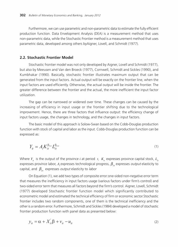
302 Bulletin of Monetary Economics and Banking, January 2012
Furthermore, we can use parametric and non-parametric data to estimate the fully efficient
production function. Data Envelopment Analysis (DEA) is a measurement method that usesnon-parametric data, while the Stochastic Frontier method is a measurement method that uses
parametric data, developed among others byAigner, Lovell, and Schmidt (1977).
2.2. Stochastic Frontier Model
Stochastic frontier model was not only developed by Aigner, Lovell and Schmidt (1977),
but also by Meeusen and Van den Broeck (1977), Cornwell, Schmidt and Sickles (1990), andKumbhakar (1990). Basically, stochastic frontier illustrates maximum output that can be
generated from the input factors. Actual output will be exactly on the frontier line, when the
input factors are used efficiently. Otherwise, the actual output will be inside the frontier. Thegreater difference between the frontier and the actual, the more inefficient the input factor
utilization.
The gap can be narrowed or widened over time. These changes can be caused by the
increasing of efficiency in input usage or the frontier shifting due to the technologicalimprovement. Hence, there are three factors that influence output: the efficiency change of
input factors usage, the changes in technology, and the changes in input factors.
The basic model of this approach is Solow-Swan based on the Cobb-Douglas productionfunction with stock of capital and labor as the input. Cobb-Douglas production function can be
expressed as:
(1)
(2)
Where Yit is the output of the province i at period t, K
it expresses province capital stock, L
it
expresses province labor, At expresses technological progress, β
1it expresses output elasticity to
capital, and β2it
expresses output elasticity to labor
On Equation (1), we add two types of composite error:one-sided non-negative error termthat measures the inefficiency in input factors usage (various factors under firm»s control) and
two-sided error term that measures all factors beyond the firm»s control. Aigner, Lovell, Schmidt
(1977) developed Stochastic frontier function model which significantly contributed toeconometric model and estimated the technical efficiency of firm or economic sector.Stochastic
frontier includes two random components, one of them is the technical inefficiency and the
other is a random error. Furthermore, Schmidt and Sickles (1984) developed a model of stochasticfrontier production function with panel data as presented below:
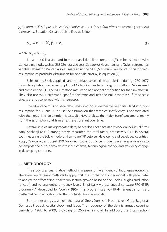
303Analysis of Sectoral Efficiency and the Response of Regional Policy
(3)
Where α 1 = α
- u
it
Equation (3) is a standard form on panel data literatures, and β can be estimated withstandard methods, such as GLS (Generalized Least Square) or Haussmann and Taylor instrumental
variables estimator. We can also estimate using the MLE (Maximum Likelihood Estimator) with
assumption of particular distribution for one side error uit in equation (2).
Schmidt and Sickles applied panel model above on airline sample data during 1970-1977
(prior deregulation) under assumption of Cobb-Douglas technology. Schmidt and Sickles used
and compare the GLS and MLE method (assuming half normal distribution for the firm effects).They also use Wu-Haussmann specification error and test the null hypothesis: firm-specific
effects are not correlated with its regressor.
The advantage of using panel data is we can choose whether to use a particular distribution
assumption for v and u or use the assumption that technical inefficiency is not correlatedwith the input. This assumption is testable. Nevertheless, the major benefitsncome primarily
from the assumption that firm effects are constant over time.
Several studies use aggregated data, hence does not necessarily work on individual firmsdata. Senhadji (2000) among others measured the total factor productivity (TFP) in several
countries using the Solow model and compare TFP between developing and developed countries.
Koop, Osiewalski, and Steel (1997) applied stochastic frontier model using Bayesian analysis todecompose the output growth into input change, technological change and efficiency change
in developing countries.
III. METHODOLOGY
This study uses quantitative method in measuring the efficiency of Indonesia»s economy.
There are two different methods to apply, first, the stochastic frontier model with panel data,to analyzethe effect of input factor on sectoral growth based on the Cobb-Douglas production
function and to analyzethe efficiency levels. Empirically we use special software FRONTIER
program 4.1 developed by Coelli (1996). This program use FORTRAN language to insertmathematical specification into the stochastic frontier models.
For frontier analysis, we use the data of Gross Domestic Product, real Gross Regional
Domestic Product, capital stock, and labor. The frequency of the data is annual, covering
periods of 1985 to 2009, providing us 25 years in total. In addition, the cross section
yit is output, X is input, v is statistical noise, and u > 0 is a firm effect representing technical
inefficiency. Equation (2) can be simplified as follow:

304 Bulletin of Monetary Economics and Banking, January 2012
identifier is nine sectors of the economy (Table 1). In total, the number of sample data is225.
We refer to the Solow-Swan model with the basic Cobb-Douglas production function.
Recall Equation (1), the function to estimate is . Where Yit is GDP or real
regional GDP of province i to time t; Kit is capital stock of province i to time t; L
it is labor of
province i to time t; At is similar to Aeξt, where ξ measures the rate of technical progress; β
1,it
is the level of output elasticity to capital; and β2, it
the level of output elasticity to labor.
We apply this model on several provinces, including North Sumatera, South Sumatera,
West Java, Central Java, East Java, Bali, South Kalimantan, and South Sulawesi.
IV. RESULTS AND ANALYSIS
4.1. Sectoral Economic Profile in Regional and National Level
The GDP growth is contributed by nine sectors. Four major sectors with the totalcontribution of 68.2% are Manufacturing, Trade Hotel and Restaurant, Agriculture, and Mining
sector with the individual share of 27.8%, 15.5%, 14.5%, and 10.4% respectively. With this
significant contribution, the movement of total GDP growth will depends mainly on these foursectors.
The regional economic growth contributes variously to national growth. Some regional
growths coincide with the national growth, and some are even higher than the national level.However, there are regions with lower growth than the national. The different growth between
regional and national may arise from different sectoral economic structure. This occur in Riau,
Table 1.Economic Sector
No S e c t o r
1 Agricultural
2 Mining sector
3 Manufacturing
4 Electricity, Gas, and Water
5 Construction
6 Trade, Hotel and Restaurant
7 Transport and Telecommunications
8 Financial
9 Service
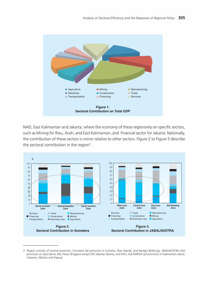
305Analysis of Sectoral Efficiency and the Response of Regional Policy
NAD, East Kalimantan and Jakarta, where the economy of these regionsrely on specific sectors,
such as Mining for Riau, Aceh, and East Kalimantan, and financial sector for Jakarta. Nationally,
the contribution of these sectors is minor relative to other sectors. Figure 2 to Figure 5 describethe sectoral contribution in the region3.
Figure 1.Sectoral Contribution on Total GDP
Agriculture Mining Manufacturing
Electricity Construction Trade
Transportation Financing Services
3 Region consists of several provinces, Sumatera (all provinces in Sumatra, Riau Islands, and Bangka Belitung); JABALNUSTRA (theprovinces on Java Island, Bali, Nusa Tenggara except DKI Jakarta) Jakarta, and KALI_SULAMPUA (all provinces in Kalimantan island,Sulawesi, Maluku and Papua)
Figure 2.Sectoral Contribution in Sumatera
Figure 3.Sectoral Contribution in JABALNUSTRA
0
10
20
30
40
50
60
70
80
90
100
%
North SumatraZone
Central SumatraZone
South SumatraZone
Services
Financing
Transportation
Trade
Construction
Electricity, Gas
Manufacturing
Mining
Agriculture
Services
Financing
Transportation
Trade
Construction
Electricity, Gas
Manufacturing
Mining
Agriculture
0
10
20
30
40
50
60
70
80
90
100
West JavaZone
Central JavaZone
East JavaZone
Bali NustengZone
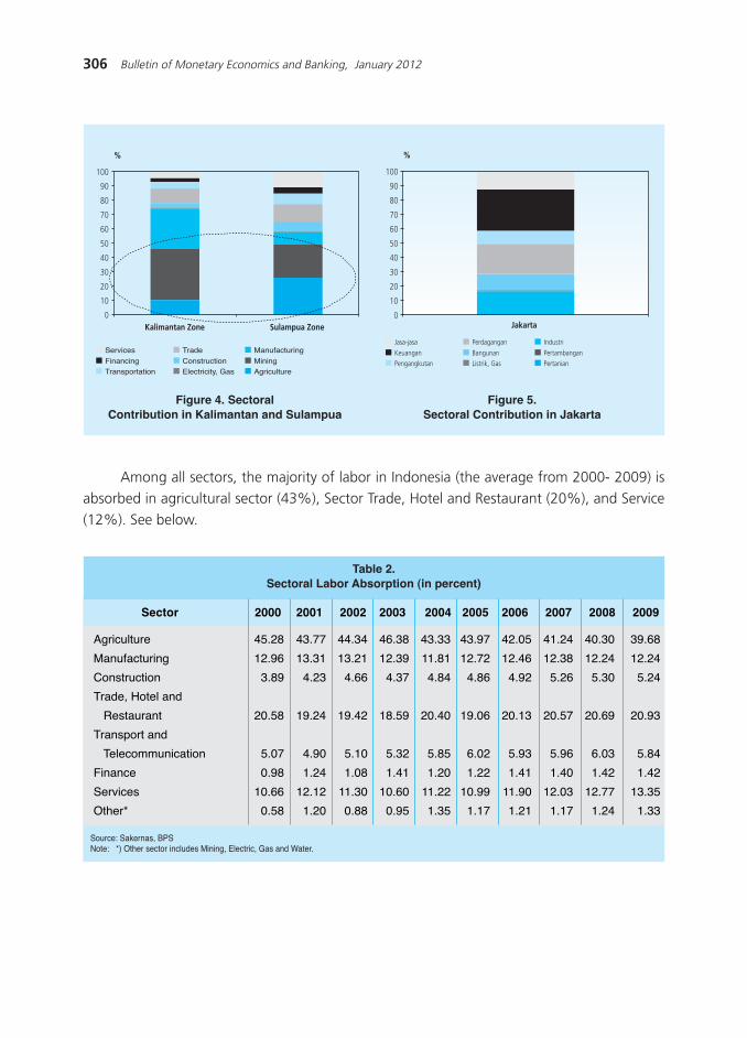
306 Bulletin of Monetary Economics and Banking, January 2012
Among all sectors, the majority of labor in Indonesia (the average from 2000- 2009) is
absorbed in agricultural sector (43%), Sector Trade, Hotel and Restaurant (20%), and Service
(12%). See below.
Figure 4. SectoralContribution in Kalimantan and Sulampua
Figure 5.Sectoral Contribution in Jakarta
%
0
10
20
30
40
50
60
70
80
90
100
Kalimantan Zone Sulampua Zone
Services
Financing
Transportation
Trade
Construction
Electricity, Gas
Manufacturing
Mining
Agriculture
Jakarta0
10
20
30
40
50
60
70
80
90
100
%
Jasa-jasa
KeuanganPengangkutan
Perdagangan
BangunanListrik, Gas
Industri
PertambanganPertanian
Table 2.Sectoral Labor Absorption (in percent)
Sector 2000 2001 2002 2003 2004 2005 2006 2007 2008 2009
Source: Sakernas, BPSNote: *) Other sector includes Mining, Electric, Gas and Water.
Agriculture 45.28 43.77 44.34 46.38 43.33 43.97 42.05 41.24 40.30 39.68
Manufacturing 12.96 13.31 13.21 12.39 11.81 12.72 12.46 12.38 12.24 12.24
Construction 3.89 4.23 4.66 4.37 4.84 4.86 4.92 5.26 5.30 5.24
Trade, Hotel and
Restaurant 20.58 19.24 19.42 18.59 20.40 19.06 20.13 20.57 20.69 20.93
Transport and
Telecommunication 5.07 4.90 5.10 5.32 5.85 6.02 5.93 5.96 6.03 5.84
Finance 0.98 1.24 1.08 1.41 1.20 1.22 1.41 1.40 1.42 1.42
Services 10.66 12.12 11.30 10.60 11.22 10.99 11.90 12.03 12.77 13.35
Other* 0.58 1.20 0.88 0.95 1.35 1.17 1.21 1.17 1.24 1.33
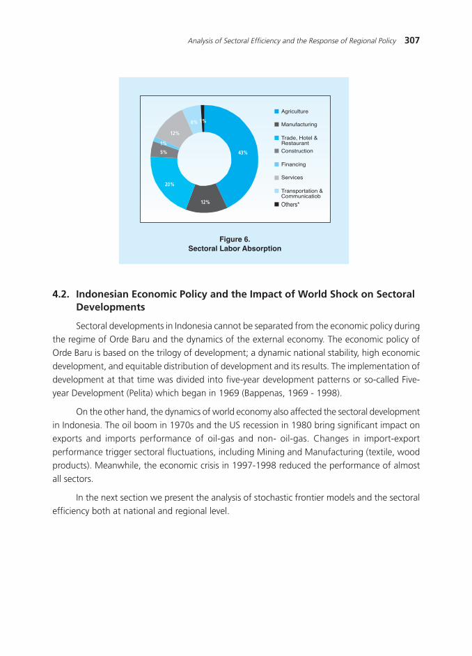
307Analysis of Sectoral Efficiency and the Response of Regional Policy
4.2. Indonesian Economic Policy and the Impact of World Shock on SectoralDevelopments
Sectoral developments in Indonesia cannot be separated from the economic policy duringthe regime of Orde Baru and the dynamics of the external economy. The economic policy of
Orde Baru is based on the trilogy of development; a dynamic national stability, high economic
development, and equitable distribution of development and its results. The implementation ofdevelopment at that time was divided into five-year development patterns or so-called Five-
year Development (Pelita) which began in 1969 (Bappenas, 1969 - 1998).
On the other hand, the dynamics of world economy also affected the sectoral developmentin Indonesia. The oil boom in 1970s and the US recession in 1980 bring significant impact on
exports and imports performance of oil-gas and non- oil-gas. Changes in import-export
performance trigger sectoral fluctuations, including Mining and Manufacturing (textile, woodproducts). Meanwhile, the economic crisis in 1997-1998 reduced the performance of almost
all sectors.
In the next section we present the analysis of stochastic frontier models and the sectoral
efficiency both at national and regional level.
Figure 6.Sectoral Labor Absorption
Agriculture
Manufacturing
Trade, Hotel &Restaurant
Construction
Financing
Services
Transportation &Communicatiob
Others*
43%
12%
20%
5%
1%
12%
6% 1%

308 Bulletin of Monetary Economics and Banking, January 2012
Figure 7.Event Analysis
Table 3.Indonesia’s Economic Policy
PELITA TARGET POLICY
I(1969-1974)
II(1974-1979
III(1979 – 1984)
IV(1984 – 1989)
V(1989-1994)
VI(1994-1998)
RPJM
The central point of development isAgriculture (food production), supported byclothing, infrastructure, and other sectors tosupport Agriculture.
Availability of food, clothing, housing, andinfrastructure
Focus on equity (world economic recession ,1980)
The agricultural sector towards food self-sufficiency and industrial development thatcan produce own machine
Food self-sufficiency and industrialdevelopment
Food self-sufficiency and industrialdevelopment
-
Focus on policies to boost rice production(agricultural intensification) and infrastruc-ture improvements, as well as the ease ofinvestment
Continuity of agricultural intensification andextensification, ease on Mining investment
the policies for Industrial development
the policy of bank liberalization,Pakto 1988
Deregulation on trade policy (1992)
-
The era of low cost carrier in air transport
1969,Intensification
and extensificationon Agriculture
1988;Deregulation
on capital andinsurance market
1980;US economic
recession
1984-1987;Trade
deregulationand investment
1969; the start of PELITA
and the ease offoreign investment.
1998;economic
crisis in Asia
1990-1993;tariff reduction
2000-2003; InflationTargeting Frameworkand trade deregulation
-15.0
-10.0
-5.0
0.0
5.0
10.0
15.0
Growth
19611963
19651967
19691971
19731975
19771979
19811983
19851987
19891991
19931995
19971999
20012003
20052007
2009

309Analysis of Sectoral Efficiency and the Response of Regional Policy
4.3. Analysis of Stochastic Frontier
By using panel data, we will outline the aggregate elasticity of input factor, while the
level of efficiency will be analyzed on sectoral level. Generally, the level of sectoral efficiency
changes over time or time varying, with an increasing trend.
4.3.1. Input Factor Analysis at National Level
This study emphasizes the role of input factors on producing the output, without analyzingtheir quality. This is consistent with the Neo Classic theory, which considers only the accumulation
of input factor (capital stock and labor). The empirical results of Stochastic Frontier with Maximum
Likelihood Estimator (MLE) method is:
Log (likelihood) = 309.37
The above is a result from panel data regression with nine economic sectors during 1985-
2009. Nationally, the elasticity of capital and labor are 0.20 and 0.34 respectively, with a fairly
high significance level ( ). These are consistent with Tjahjono and Anugrah (2006) that the roleof labor is greater than the capital stock for Indonesian economy.
The labor elasticity of 0.34 indicates a 1% increase of labor will increase the output by
0.34%. Meanwhile, an increase of 1 unit of capital will increase output by 0.2 units, which
mean to increase 1 unit of output require 5 additional units of capital. On the other hand, theIncremental Capital Output Ratio (ICOR) during 2008-2009is 4-5, which represents the needs
of 4-5 additional units of capital to increase the output by 1 unit.
4.3.2. Regional Input Factor Analysis
The results of regional input factor analysis are presented in Table 5.1. Depends on thecharacteristic of regional economy, the proportion of capital stock and labor factor varies across
region.
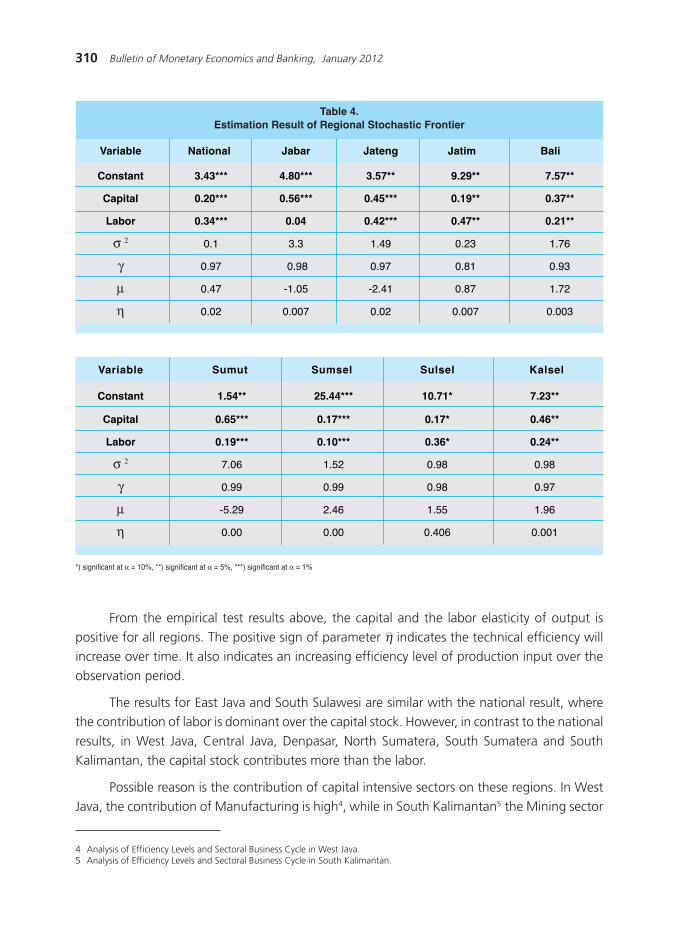
310 Bulletin of Monetary Economics and Banking, January 2012
From the empirical test results above, the capital and the labor elasticity of output is
positive for all regions. The positive sign of parameter η indicates the technical efficiency willincrease over time. It also indicates an increasing efficiency level of production input over the
observation period.
The results for East Java and South Sulawesi are similar with the national result, wherethe contribution of labor is dominant over the capital stock. However, in contrast to the national
results, in West Java, Central Java, Denpasar, North Sumatera, South Sumatera and South
Kalimantan, the capital stock contributes more than the labor.
Possible reason is the contribution of capital intensive sectors on these regions. In WestJava, the contribution of Manufacturing is high4, while in South Kalimantan5 the Mining sector
Table 4.Estimation Result of Regional Stochastic Frontier
Variable National Jabar Jateng Jatim Bali
Constant 3.43*** 4.80*** 3.57** 9.29** 7.57**
Capital 0.20*** 0.56*** 0.45*** 0.19** 0.37**
Labor 0.34*** 0.04 0.42*** 0.47** 0.21**
σ 2 0.1 3.3 1.49 0.23 1.76
γ 0.97 0.98 0.97 0.81 0.93
μ 0.47 -1.05 -2.41 0.87 1.72
η 0.02 0.007 0.02 0.007 0.003
*) significant at α = 10%, **) significant at α = 5%, ***) significant at α = 1%
Variable Sumut Sumsel Sulsel Kalsel
Constant 1.54** 25.44*** 10.71* 7.23**
Capital 0.65*** 0.17*** 0.17* 0.46**
Labor 0.19*** 0.10*** 0.36* 0.24**
σ 2 7.06 1.52 0.98 0.98
γ 0.99 0.99 0.98 0.97
μ -5.29 2.46 1.55 1.96
η 0.00 0.00 0.406 0.001
4 Analysis of Efficiency Levels and Sectoral Business Cycle in West Java.5 Analysis of Efficiency Levels and Sectoral Business Cycle in South Kalimantan.
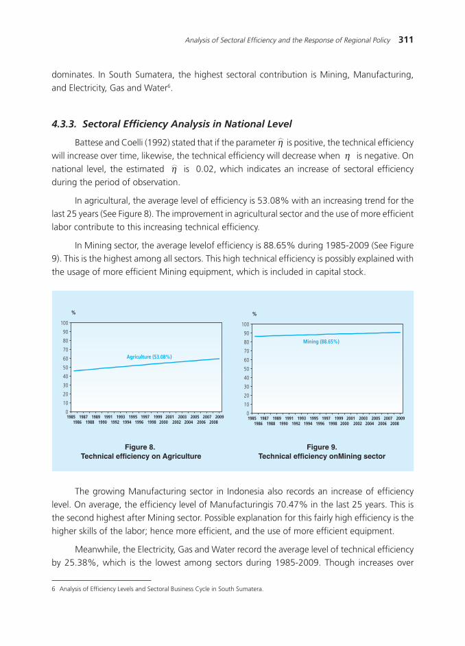
311Analysis of Sectoral Efficiency and the Response of Regional Policy
%
Mining (88.65%)
0
10
20
30
40
50
60
70
80
90
100
19851986
19871988
19891990
19911992
19931994
19951996
19971998
19992000
20012002
20032004
20052006
20072008
2009
dominates. In South Sumatera, the highest sectoral contribution is Mining, Manufacturing,
and Electricity, Gas and Water6.
4.3.3. Sectoral Efficiency Analysis in National Level
Battese and Coelli (1992) stated that if the parameter η is positive, the technical efficiencywill increase over time, likewise, the technical efficiency will decrease when η is negative. On
national level, the estimated η is 0.02, which indicates an increase of sectoral efficiency
during the period of observation.
In agricultural, the average level of efficiency is 53.08% with an increasing trend for thelast 25 years (See Figure 8). The improvement in agricultural sector and the use of more efficient
labor contribute to this increasing technical efficiency.
In Mining sector, the average levelof efficiency is 88.65% during 1985-2009 (See Figure9). This is the highest among all sectors. This high technical efficiency is possibly explained with
the usage of more efficient Mining equipment, which is included in capital stock.
6 Analysis of Efficiency Levels and Sectoral Business Cycle in South Sumatera.
Figure 8. Technical efficiency on Agriculture
Figure 9.Technical efficiency onMining sector
%
Agriculture (53.08%)
0
10
20
30
40
50
60
70
80
90
100
19851986
19871988
19891990
19911992
19931994
19951996
19971998
19992000
20012002
20032004
20052006
20072008
2009
The growing Manufacturing sector in Indonesia also records an increase of efficiencylevel. On average, the efficiency level of Manufacturingis 70.47% in the last 25 years. This is
the second highest after Mining sector. Possible explanation for this fairly high efficiency is the
higher skills of the labor; hence more efficient, and the use of more efficient equipment.
Meanwhile, the Electricity, Gas and Water record the average level of technical efficiencyby 25.38%, which is the lowest among sectors during 1985-2009. Though increases over

312 Bulletin of Monetary Economics and Banking, January 2012
%
Construction (55.17%)
0
10
20
30
40
50
60
70
80
90
100
19851986
19871988
19891990
19911992
19931994
19951996
19971998
19992000
20012002
20032004
20052006
20072008
2009
%
Trade, Hotel and Restaurant (58.50%)
0
10
20
30
40
50
60
70
80
90
100
19851986
19871988
19891990
19911992
19931994
19951996
19971998
19992000
20012002
20032004
20052006
20072008
2009
%
Manufacturing (70.47%)
0
10
20
30
40
50
60
70
80
90
100
19851986
19871988
19891990
19911992
19931994
19951996
19971998
19992000
20012002
20032004
20052006
20072008
2009
%
Electricity, gas and water (25.38%)
0
10
20
30
40
50
60
70
80
90
100
19851986
19871988
19891990
19911992
19931994
19951996
19971998
19992000
20012002
20032004
20052006
20072008
2009
time, the low efficiency level of this sector is possibly caused by the less efficient of its production
equipment.
Figure 10.Technical efficiency on Manufacturing
Figure 11.Technical efficiency on Electric, Gas and Water
The average level of technical efficiency on Construction also increases over time.The
technical efficiency in this sector is averagely 55.17% for the last 25 years. The efficiencyincrease in this sector is relatively higher as illustrated with steeper line in Figure 12.
Trading, Hotels and Restaurants records 58.50% of efficiency level for the same period;
similar with the Construction sector. The efficiency level in this sector is also changing over time
with a positive trend. The more efficient the labor, the higher the technical efficiency of thissector.
Figure 12.Technical efficiency on Construction
Figure 13. Technical efficiency
Sector on Trade, Hotel and Restaurant

313Analysis of Sectoral Efficiency and the Response of Regional Policy
%
Services (43.99%)
0
10
20
30
40
50
60
70
80
90
100
19851986
19871988
19891990
19911992
19931994
19951996
19971998
19992000
20012002
20032004
20052006
20072008
2009
%
Transport and Telecomunication (43.40%)
0
10
20
30
40
50
60
70
80
90
100
19851986
19871988
19891990
19911992
19931994
19951996
19971998
19992000
20012002
20032004
20052006
20072008
2009
%
Finance (65.93%)
0
10
20
30
40
50
60
70
80
90
100
19851986
19871988
19891990
19911992
19931994
19951996
19971998
19992000
20012002
20032004
20052006
20072008
2009
The efficiency level of Transport and Telecommunication changes over time with a positive
trend. However, the average efficiency level is quite low, 43.40% during 1985-2009. The useof inefficient supporting equipment on Transport is possible reason for its low efficiency.
In financial sector, the average level of efficiency during the period 1985-2009 is 65.93%.
Several financial policies including banking policy of Pakto 1988 increase the performance ofthis sector. In addition, the labor of this sector tends to be more efficient. Over time, the
efficiency of Financial sector also increases.
Figure 14. Technical efficiencyon Transport and Telecommunication
Figure 15.Technical efficiency on Financial Sector
Service sector also records a change in technical efficiency over time, with a positivetrend. However, the average level of efficiency for this sector is low, 43.99%, for the last 25
years. Consideringits changes rate, the technical efficiency of this sector increases rapidly, as
indicated by steeper line in Figure 16.
Figure 16.Technical efficiency on Service Sector
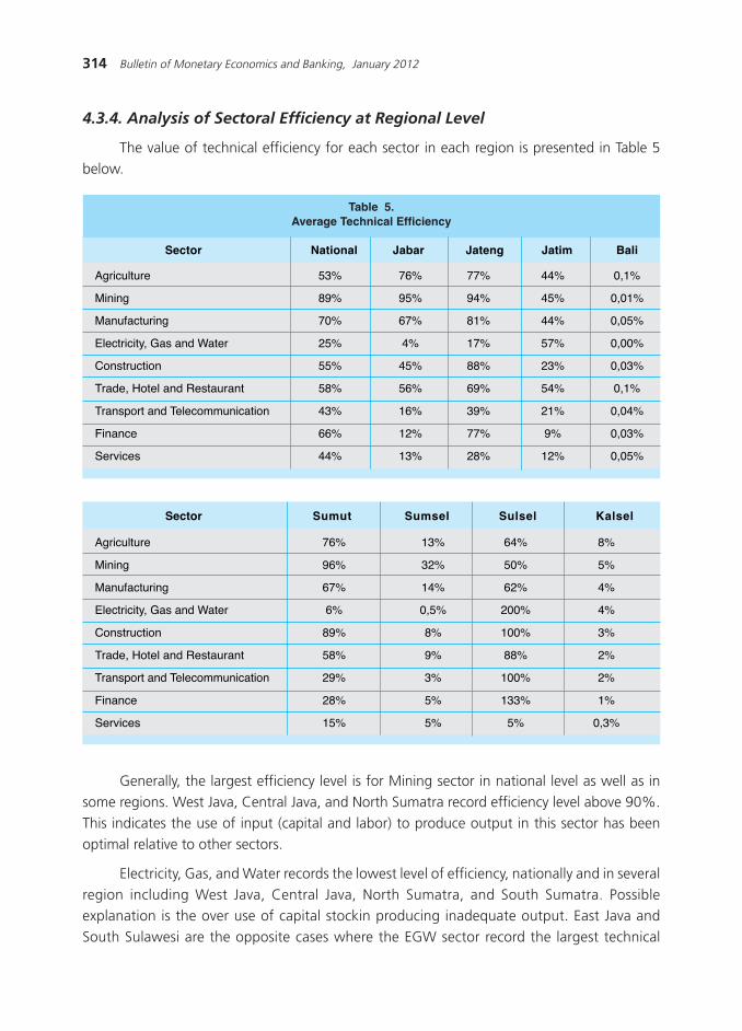
314 Bulletin of Monetary Economics and Banking, January 2012
4.3.4. Analysis of Sectoral Efficiency at Regional Level
The value of technical efficiency for each sector in each region is presented in Table 5
below.
Table 5.Average Technical Efficiency
Sector National Jabar Jateng Jatim Bali
Agriculture 53% 76% 77% 44% 0,1%
Mining 89% 95% 94% 45% 0,01%
Manufacturing 70% 67% 81% 44% 0,05%
Electricity, Gas and Water 25% 4% 17% 57% 0,00%
Construction 55% 45% 88% 23% 0,03%
Trade, Hotel and Restaurant 58% 56% 69% 54% 0,1%
Transport and Telecommunication 43% 16% 39% 21% 0,04%
Finance 66% 12% 77% 9% 0,03%
Services 44% 13% 28% 12% 0,05%
Sector Sumut Sumsel Sulsel Kalsel
Agriculture 76% 13% 64% 8%
Mining 96% 32% 50% 5%
Manufacturing 67% 14% 62% 4%
Electricity, Gas and Water 6% 0,5% 200% 4%
Construction 89% 8% 100% 3%
Trade, Hotel and Restaurant 58% 9% 88% 2%
Transport and Telecommunication 29% 3% 100% 2%
Finance 28% 5% 133% 1%
Services 15% 5% 5% 0,3%
Generally, the largest efficiency level is for Mining sector in national level as well as in
some regions. West Java, Central Java, and North Sumatra record efficiency level above 90%.
This indicates the use of input (capital and labor) to produce output in this sector has beenoptimal relative to other sectors.
Electricity, Gas, and Water records the lowest level of efficiency, nationally and in several
region including West Java, Central Java, North Sumatra, and South Sumatra. Possibleexplanation is the over use of capital stockin producing inadequate output. East Java and
South Sulawesi are the opposite cases where the EGW sector record the largest technical
315Analysis of Sectoral Efficiency and the Response of Regional Policy
efficiency; hence most efficient. Furthermore, In East Java7 the amount of labor has been
considered to be optimal.
V. CONCLUSION
Since the regime of Orde Baru, the government has been trying to encourage the sectoralgrowth as a part of the overall economic development. Some fundamental policies have
improvedthe sectoral performance, including intensification and extensification policy, which
has increased the growth on Agricultural sector, especially food which contribute 60%. Infinancial sector, the enactment of Pakto 1988 and its continuous policy package had raised the
financial sector performance, originated from banking. In Manufacturing, the policy, which
focuses on the clothes availability and supported by industrial regulation, particularly oninvestment, has increased the TPT performance.
This paper provides two important findings. First, with additional information on the
technical efficiency of input, the stochastic frontier model is better than the Solow-Swan model.
The estimated shares of capital stock and labor are 0.20 and 0.34 respectively. This indicatesthe labor dominates of the use of capital stock in Indonesia»s economy.
Second, all sectors experienced an increase of technical efficiency during period of 1985-
2009. The Mining sector on average has the highest technical efficiency (88.65%), followed byManufacturing sector (70.47%) and Financial sector (65.93%). While the Electricity, Gas, and
Water recorded the lowest average efficiency by 25.38%, for the last 25 years.
These two findings require the government role to raise the level of efficiency especiallyin some sectors with low efficiency such as Electricity, Gas, and Water. Since the government
dominate this sector, it is important to provide incentives for the state owned company to
increase their efficiency.
This research calls for further research by examining the quality of input factor for eachsector, such as human capital and the term structure of the capital. In addition, it is also important
to include the sectoral Total Factor Productivity (TFP).
7 Analysis of Sectoral Efficiency Level and Sectoral Business Cycle in East Java
316 Bulletin of Monetary Economics and Banking, January 2012
Afonso, Antonio, Davide, Furceri, 2007. Sectoral Business Cycle Synchronization in the EuropeanUnion, Portugal, UECE
Bry, Gerhard, Boschan, Charlotte, 1971. Cyclical Analysis of Time Series-Selected procedureand Computer Programs, NBER.
Burns, Arthur F and Mitchell, Wesley C, 1946. Measuring Business Cycle, New York, NBER.
Cecchetti, Stephen G et.al. 2001-2002. Assessing the Sources of Changes in the Volatility ofReal Growth, paper on Business Cycle Conference in Sydney, RBA.
Bappenas, 1969 - 1999. Dokumen Buku Rencana Pembangunan Lima Tahun (REPELITA),BAPPENAS Jakarta.
Evert, Martin, 2006. Sectoral and Industrial Business Cycles, University of Bern, Germany, MPRApaper No.1176
Harmanta, Bathaluddin M. Barik, Waluyo Jati, 2010 ARIMBI with Imperfect Credibility, Working
Paper No. WP/03/2010, Jakarta, Bank Indonesia.Hong, Kiseok, Lee, Jong-Wha, Tang, Hsiao, Chink, 2009, Crises in Asia: Historical Perspectives
and Implications, ABD Economic Working Paper Series No. 152, Asean Development Bank,
Manila.Ligaya Clarita, Majid M Abdul, Rendra Z Idris, 2004, Penyempurnaan Leading
IndikatordanPenerapan Markov Switching untuk Mendeteksi Titik balik secara Real Time,
SSR-DKMNguyen, Toan, 2007, Determinants of Business Cycle Synchronization in East Asia: An Extreme
Bound Analysis, Depocen, Kyoto-Japan.
Pindyck, Robert, Rubinfeld, Daniel, 1997, Economic Models and Econometric Forecasts, NewYork, McGraw-Hill, 4th ed.
Thimann, Christian, 2004, Real Convergence, Economic Dynamics, and the Adoption of the
Euro in the New European Union Member States, presentation at the International MonetaryFund Conference in Prague.
REFERENCES

317Analysis of Sectoral Efficiency and the Response of Regional Policy
APPENDIX: SPENCER CURVE
Spencer Moving Average is generally used as a data smoothing process, to display the
underlying pattern (signal) while reducing the random fluctuation (noise). Spencer (1904)
proposed a method to remove trends from time series data by using moving average line.Spencer formulated 15 periods moving average, with negative weight for the end of period.
The Spencer Curve is particularly calculated based on the 5x5x4x4 moving average, which is
the 4 periods moving average of original data is processed using 4 periods moving average,then 5 periods moving average and finally another 5 periods moving average by assigning
weights of -3/4, 3/4, 1, 3/4, and -3/4.
The following steps show how the Spencer Curve is formed:
1. Determine 4 periods moving average. The general form is as follows:
Which MA4i is the moving average for 4 periods and x
i is the value of i time series data.
2. Determine the 4 periods moving average using MA4 data.
The general form is as follows:
Or:
MA4_4i = ( x
i + 2x
i +1 + 3x
i +2 + 4x
i +3 + 3x
i +4 + 2x
i +5 + x
i +6 ) / 4
Where MA4-4i is the moving average for 4 periods from MA4 data.
3. Determining the 5 periods Moving Average using MA4_4 data.
The general form is as follows:
MA41 = ( x
1 + x
2 + x
3 + x
4 ) / 4
MA42 = ( x
2 + x
3 + x
4 + x
5 ) / 4
.
.
.
MA4i = ( x
i + x
i+1 + x
i+2 + x
i+3 ) / 4
MA4_4i = ( MA4
i + MA4
i+1 + MA4
i+2 + MA4
i+3 ) / 4
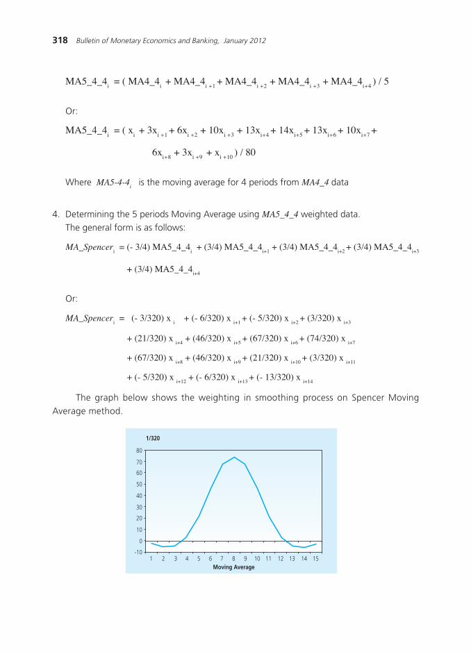
318 Bulletin of Monetary Economics and Banking, January 2012
MA5_4_4i = ( MA4_4
i + MA4_4
i +1 + MA4_4
i +2 + MA4_4
i +3 + MA4_4
i+4 ) / 5
Or:
MA5_4_4i = ( x
i + 3x
i +1 + 6x
i +2 + 10x
i +3 + 13x
i+4 + 14x
i+5 + 13x
i+6 + 10x
i+7 +
6xi+8
+ 3xi +9
+ xi +10
) / 80
Where MA5-4-4i is the moving average for 4 periods from MA4_4 data
4. Determining the 5 periods Moving Average using MA5_4_4 weighted data.
The general form is as follows:
MA_Spenceri = (- 3/4) MA5_4_4
i + (3/4) MA5_4_4
i+1 + (3/4) MA5_4_4
i+2 + (3/4) MA5_4_4
i+3
+ (3/4) MA5_4_4
i+4
Or:
MA_Spenceri = (- 3/320) x
i + (- 6/320) x
i+1 + (- 5/320) x
i+2 + (3/320) x
i+3
+ (21/320) x
i+4 + (46/320) x
i+5 + (67/320) x
i+6 + (74/320) x
i+7
+ (67/320) x
i+8 + (46/320) x
i+9 + (21/320) x
i+10 + (3/320) x
i+11
+ (- 5/320) x
i+12 + (- 6/320) x
i+13 + (- 13/320) x
i+14
The graph below shows the weighting in smoothing process on Spencer Moving
Average method.
1/320
-10
10
20
30
40
50
60
70
80
0
1 2 3 4 5 6 7 8 9 10 11 12 13 14 15Moving Average
319
WRITING GUIDANCE
1. The paper should be original and should not violate any copyrights. The submitted paper
should have never been published or not being submitted to other publisher. The copyright
of the published paper is retained to the author.
2. The Bulletin of Monetary Economics and Banking provide a financial incentive between IDR
1,000,000 to IDR 3,000,000.
3. The paper should be submitted in two formats (i) Microsoft Word (*.doc) and (ii) portable
digital file (*.PDF). These files should be sent to the following mail address:
[email protected] and Cc to: [email protected]
You may save your files in CD and send it to the following Editorial Address:
BULLETIN OF MONETARY ECONOMICS AND BANKING
Directorate of Economic Research and Monetary Policy-Bank Indonesia
Building Syafruddin Prawiranegara, 20th Floor
JI. M. H. Thamrin No.2 Central Jakarta, Indonesia
Ph. +62-21-3818202, Fax. +62-21- 3800394
4. To avoid missing fonts or other compatibility issues, any special characters or mathematical
expression (equations, symbols, matrix, etc.) must be written using Microsoft Equation.
5. The submitted paper should contain (i) an abstract of maximum one page A4, (ii) keywords
and (iii) JEL classification code. See the JEL code at http://www.aeaweb.org/journal/
jel_class_system.html.
6. The paper must contain the followings:
The background, the aim of the paper and its distinction to previous study
Theory and review of literatures
Methodology (quantitative methodology is preferred)
Result and analysis
Policy and further study implication
7. The citation should be in footnote and not in endnote.
8. The references must obey the following rule:

320 Bulletin of Monetary Economics and Banking, October 2010
a. Book:
HankeHankeHankeHankeHanke John E. John E. John E. John E. John E. and Arthur G. ReitschArthur G. ReitschArthur G. ReitschArthur G. ReitschArthur G. Reitsch, (1940), Business Forecasting, Prentice-Hall, New
Jersey.
b. Article in journal:
Rangazas, PeterRangazas, PeterRangazas, PeterRangazas, PeterRangazas, Peter. (2000) ≈Schooling and Economic Growth: A King-Rebelo Experiment
with Human Capital∆, Journal of Monetary Economics, October , 46(2), page. 397-416.
c. Article in book edited by other people:
Frankel, Jeffrey AFrankel, Jeffrey AFrankel, Jeffrey AFrankel, Jeffrey AFrankel, Jeffrey A. and Andrew K., RoseAndrew K., RoseAndrew K., RoseAndrew K., RoseAndrew K., Rose. (1995) ≈Empirical Research on Nominal Exchange
Rates∆, in Gene Grossman and Kenneth Rogoff, eds.,∆Handbook of International
Economics. Amsterdam: North-Holland, page. 397-416.
d. Working papers:
Kremer, MichaelKremer, MichaelKremer, MichaelKremer, MichaelKremer, Michael and Daniel, ChenDaniel, ChenDaniel, ChenDaniel, ChenDaniel, Chen. (2000) ≈Income Distribution Dynamics with
Endogenous Fertility∆. National Bureau of Economic Research (Cambridge, MA) Working
Paper No.7530.
e. Mimeo or unpublished work:
Knowles, JohnKnowles, JohnKnowles, JohnKnowles, JohnKnowles, John. ≈Can Parental Decision Explain U.S. Income Inequality?∆, Mimeo,
University of Pennsylvania, 1999.
f. Article from web or other electronic form:
Summers, RobertSummers, RobertSummers, RobertSummers, RobertSummers, Robert and Alan WAlan WAlan WAlan WAlan W., Heston. Heston. Heston. Heston. Heston. (1997) ≈Penn World Table, Version 5.6∆
http://pwt.econ.unpenn.edu/
g. Article in newspaper, magazine or equal periodicals:
Begley, SharonBegley, SharonBegley, SharonBegley, SharonBegley, Sharon. (1993) ≈Killed by Kindness∆, Newsweek, April 12, page. 50-56.
9. The paper should be submitted along with curriculum vitae complete with mail address and
phone number.


![Portfolio 2013 [Bayu Alfian]](https://img.pdfslide.net/doc/110x75/568bd94c1a28ab2034a686c6/portfolio-2013-bayu-alfian.jpg)