Embed Size (px)
Citation preview
Analogue and digital techniques in closed loop regulation applications
Digital systems• Sampling of analogue signals• Sample-and-hold• Parseval’s theorem
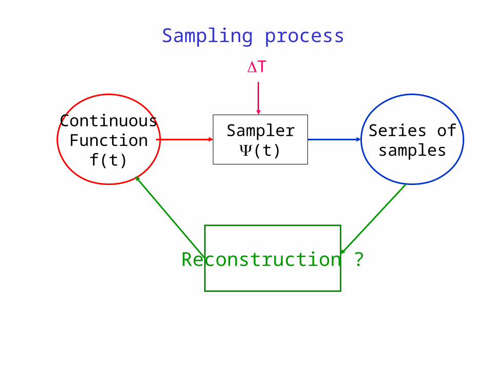
Sampling process
ContinuousFunction
f(t)
Sampler(t)
Series ofsamples
T
Reconstruction ?
From time domain to frequency domain
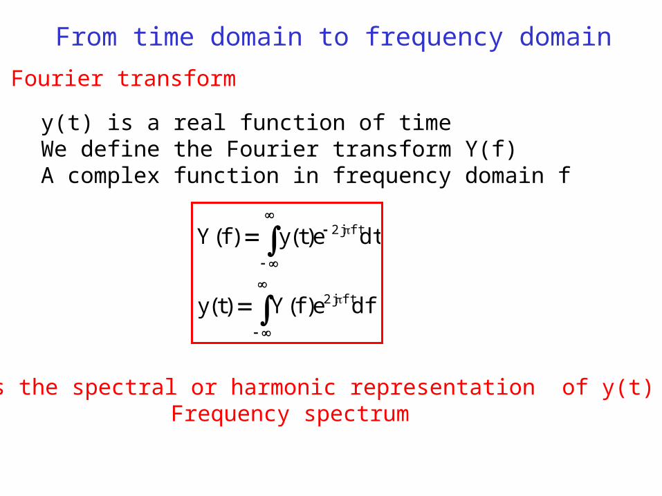
Fourier transform
y(t) is a real function of time We define the Fourier transform Y(f)A complex function in frequency domain f
dfe)f(Y)t(y
dte)t(y)f(Y
ftj2
ftj2
Y(f) is the spectral or harmonic representation of y(t) Frequency spectrum
From time domain to frequency domain
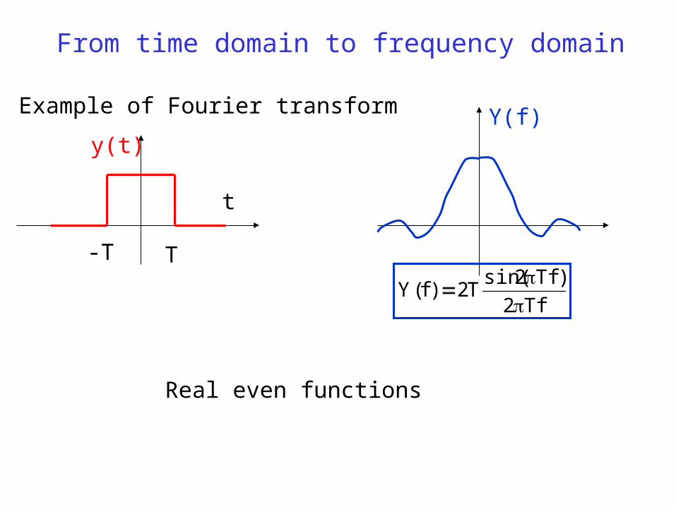
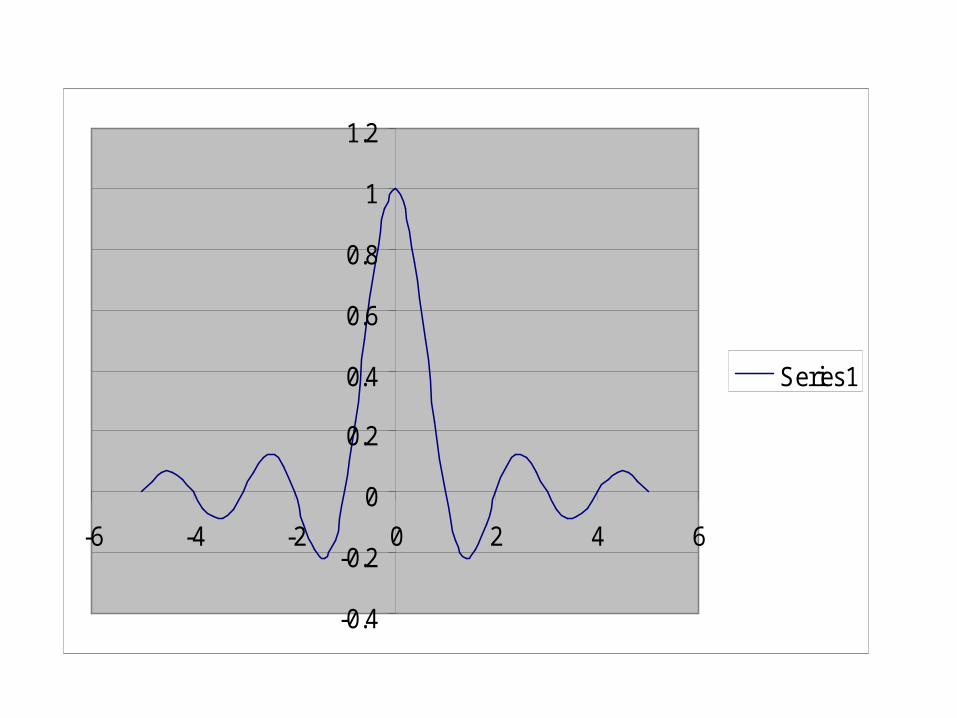
Example of Fourier transform
y(t)
t
-T T
Y(f)
Tf2
)Tf2sin(T2)f(Y
Real even functions
-0.4
-0.2
0
0.2
0.4
0.6
0.8
1
1.2
-6 -4 -2 0 2 4 6
Series1
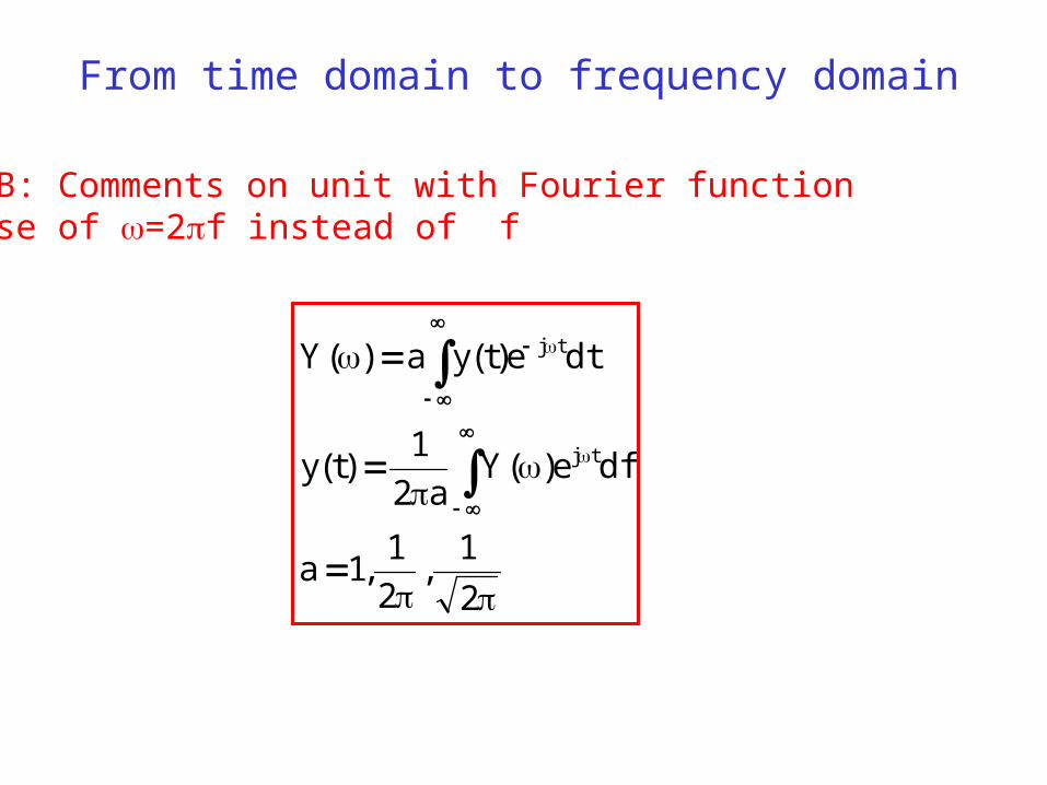
From time domain to frequency domain
NB: Comments on unit with Fourier functionUse of =2f instead of f
2
1,
2
1,1a
dfe)(Ya2
1)t(y
dte)t(ya)(Y
tj
tj
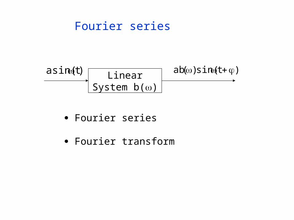
Fourier series
)tsin()(ab Linear
System b()
)tsin(a
Fourier series
Fourier transform
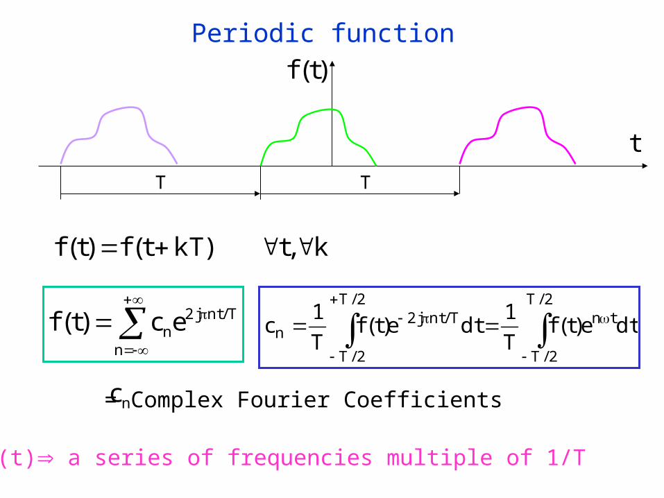
)kTt(f)t(f k,t
T/ntj2
nnec)t(f
dte)t(f
T
1dte)t(f
T
1c
2/T
2/T
tnT/ntj22/T
2/T
n
nc = Complex Fourier Coefficients
T
)t(f
t
T
Periodic function
f(t) a series of frequencies multiple of 1/T
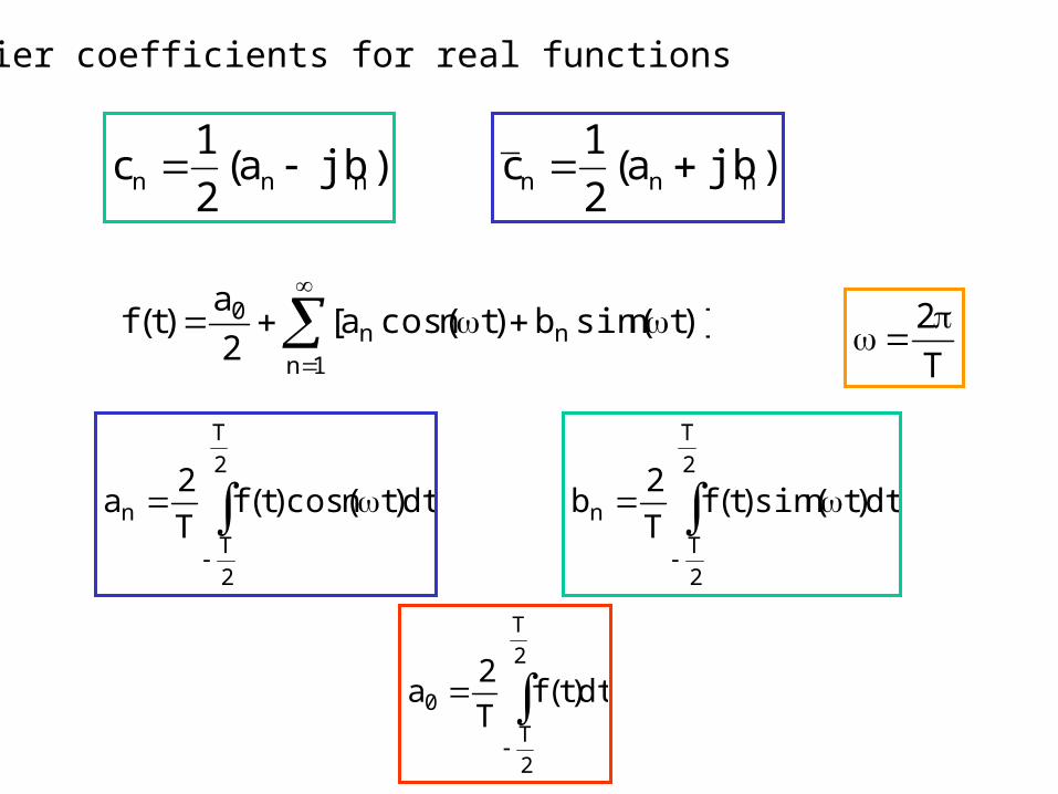
Fourier coefficients for real functions
)jba(2
1c nnn )jba(
2
1c nnn
)]tnsin(b)tncos(a[2
a)t(f n
1nn
0
dt)tncos()t(fT
2a
2
T
2
T
n
dt)t(fT
2a
2
T
2
T
0
T
2
dt)tnsin()t(fT
2b
2
T
2
T
n
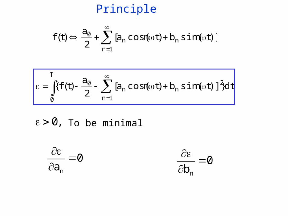
)]tnsin(b)tncos(a[2
a)t(f n
1nn
0
dt)]}tnsin(b)tncos(a[2
a)t(f{ 2
n1n
n0
T
0
,0 To be minimal
0a n
0
bn
Principle
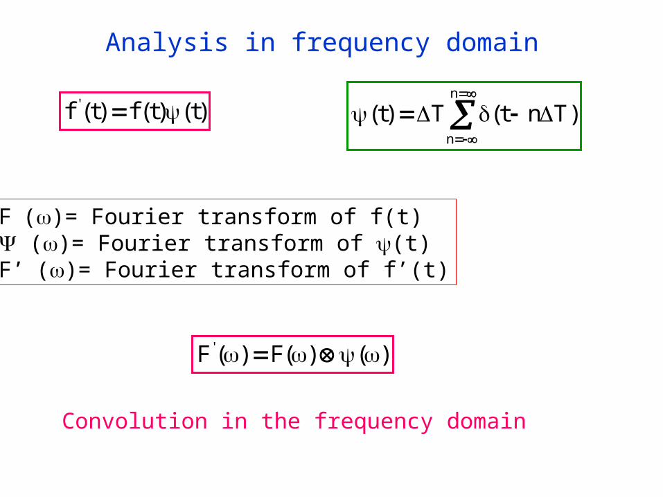
)t()t(f)t(f '
Analysis in frequency domain
n
n
)Tnt(T)t(
• F()= Fourier transform of f(t)• ()= Fourier transform of (t)• F’()= Fourier transform of f’(t)
)()(F)(F'
Convolution in the frequency domain
n
n
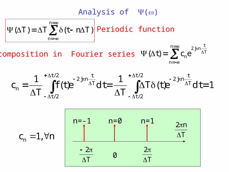
)Tnt(T)T(
Analysis of ()
1dte)t(TT
1dte)t(f
T
1c T
tnj2
2/t
2/t
T
tnj2
2/t
2/t
n
Decomposition in Fourier series
Periodic function
T
tnj2n
nnec)t(
n,1cn
n=0 n=1n=-1
T
n2
0T
2
T
2
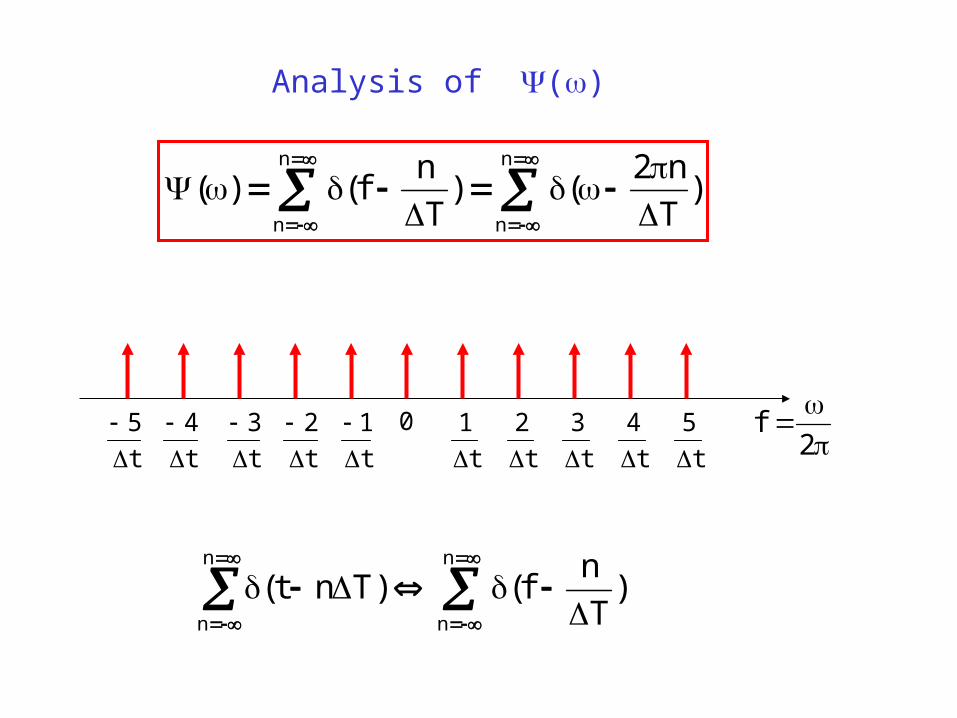
Analysis of ()
n
n
n
n
)T
n2()
T
nf()(
t
5
t
5
0
t
4
t
3
t
2
t
1
t
4
t
3
t
2
t
1
2
f
n
n
n
n
)T
nf()Tnt(
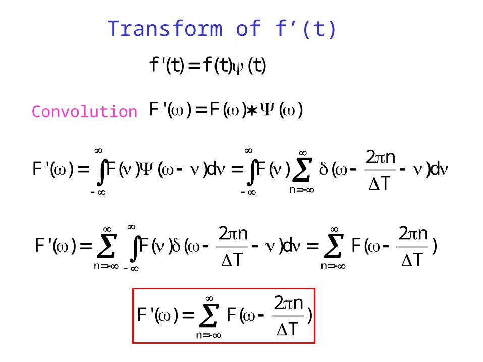
Transform of f’(t)
)t()t(f)t('f
Convolution )()(F)('F
d)T
n2()(Fd)()(F)('F
n
)T
n2(Fd)
T
n2()(F)('F
nn
)T
n2(F)('F
n
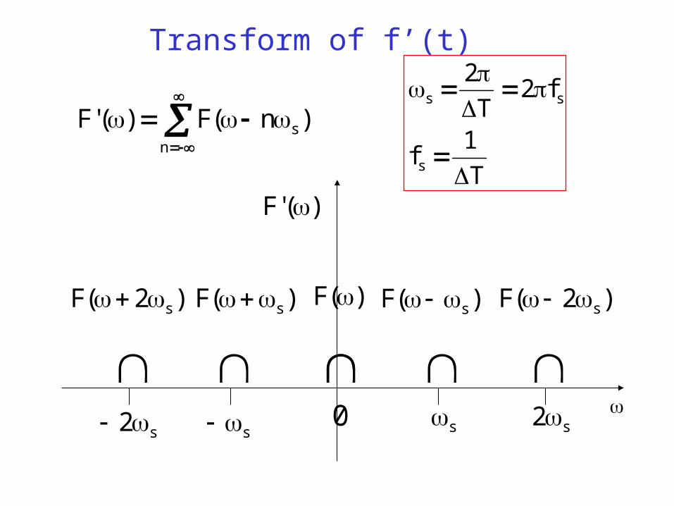
)n(F)('Fn
s
)('F
)(F )(F s
T
1f
f2T
2
s
ss
0 s
ss2 s2
)2(F s)(F s)2(F s
Transform of f’(t)
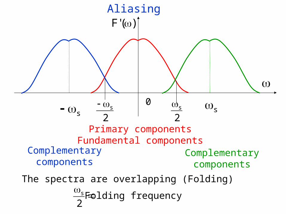
Aliasing
The spectra are overlapping (Folding)
0
Primary componentsFundamental components
ss
Complementarycomponents
Complementarycomponents
)('F
2s
2s
2
s Folding frequency
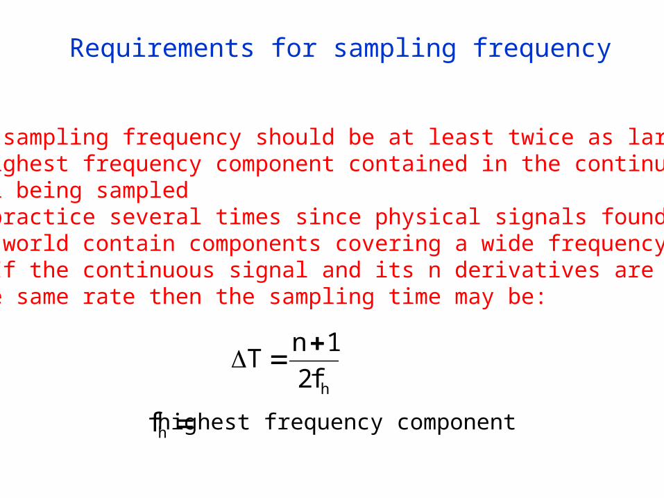
Requirements for sampling frequency
• The sampling frequency should be at least twice as large asthe highest frequency component contained in the continuoussignal being sampled• In practice several times since physical signals found in the real world contain components covering a wide frequency range •NB:If the continuous signal and its n derivatives are sampled at the same rate then the sampling time may be:
hf2
1nT
hf highest frequency component
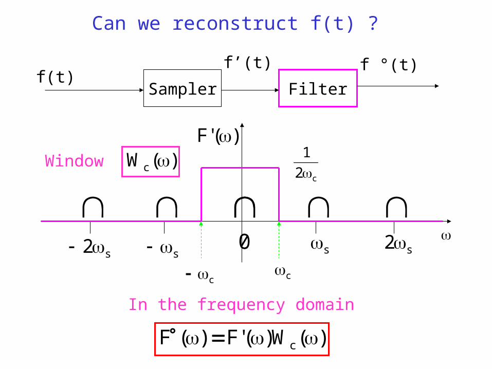
Can we reconstruct f(t) ?
Sampler Filterf(t)
f’(t) f °(t)
)(W)('F)(F c
In the frequency domain
0 s
ss2 s2
)('F
cc
Window )(Wc c2
1
)t(w)t('f)t(f c
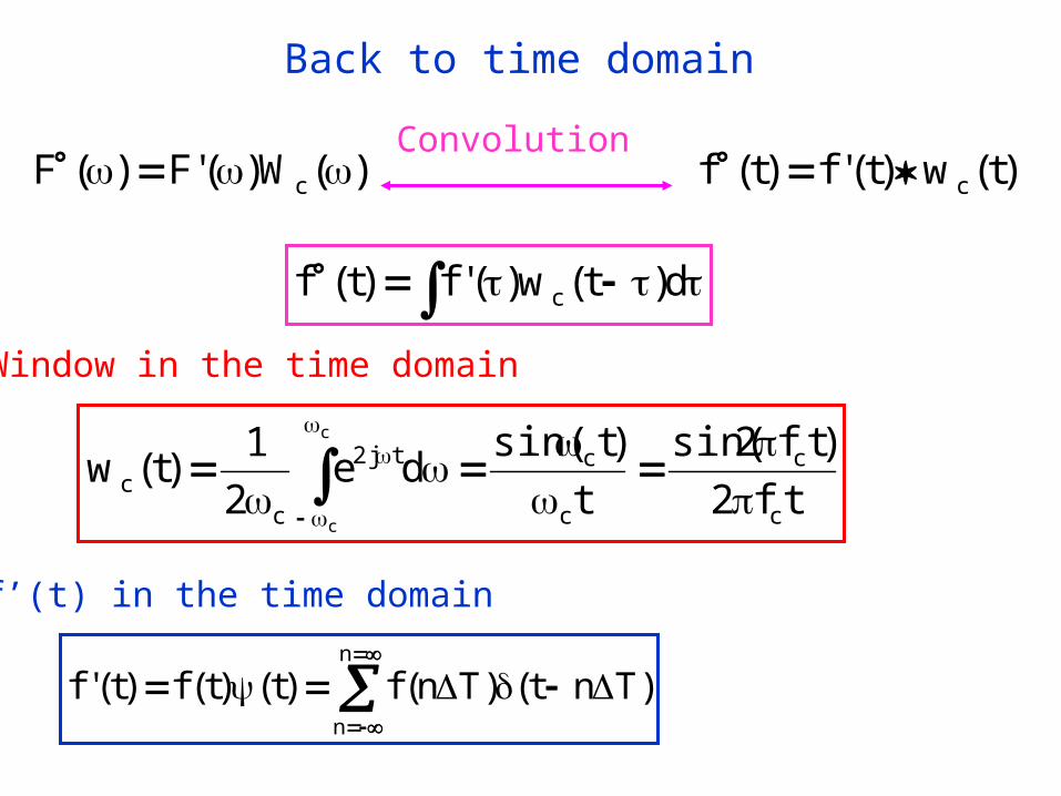
Back to time domain
)(W)('F)(F c Convolution
d)t(w)('f)t(f c
tf2
)tf2sin(
t
)tsin(de
2
1)t(w
c
c
c
ctj2
cc
c
c
Window in the time domain
n
n
)Tnt()Tn(f)t()t(f)t('f
f’(t) in the time domain
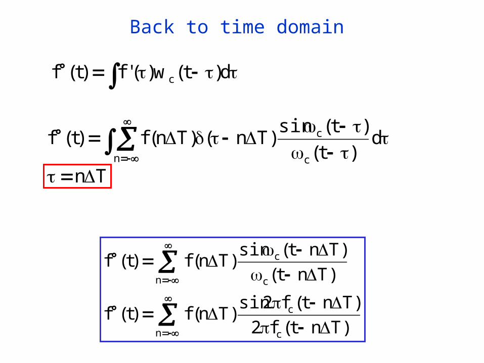
d)t(w)('f)t(f c
d)t(
)t(sin)Tn()Tn(f)t(f
c
c
n
n c
c
n c
c
)Tnt(f2
)Tnt(f2sin)Tn(f)t(f
)Tnt(
)Tnt(sin)Tn(f)t(f
Back to time domain
Tn
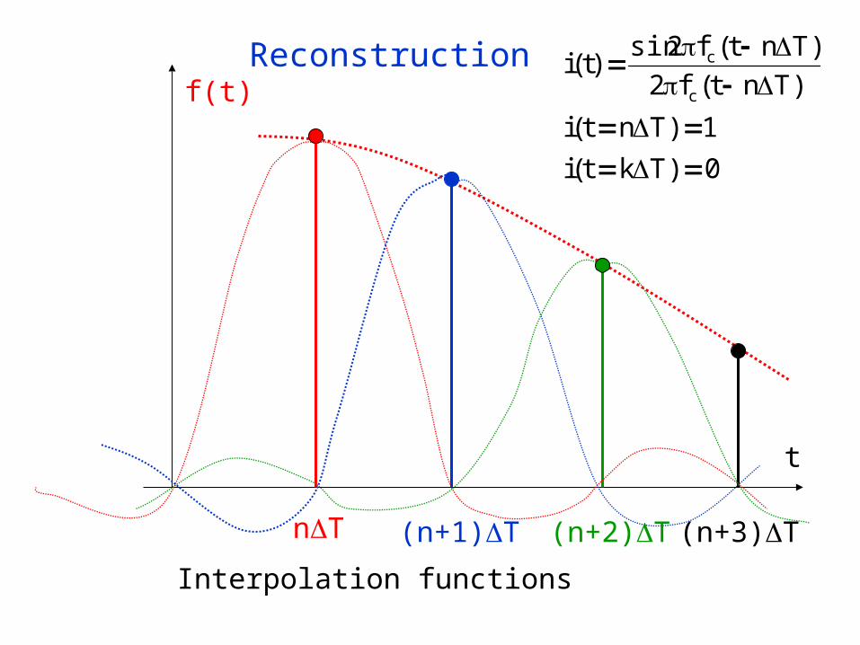
Reconstruction
t
0)Tkt(i
1)Tnt(i
)Tnt(f2
)Tnt(f2sin)t(i
c
c
f(t)
Interpolation functions
nT (n+1)T (n+2)T (n+3)T

Delayed pulse train
tT )1(T )2(T )1(T
10 T
2
n2jTnj
2
T
2
T
ntjn e
T
1e
T
1e)Tt(
T
1C
n
)Tt(jntjn
n
Tnj eee)t(
Analogue and digital techniques in closed loop regulation applications
Zero-order-hold
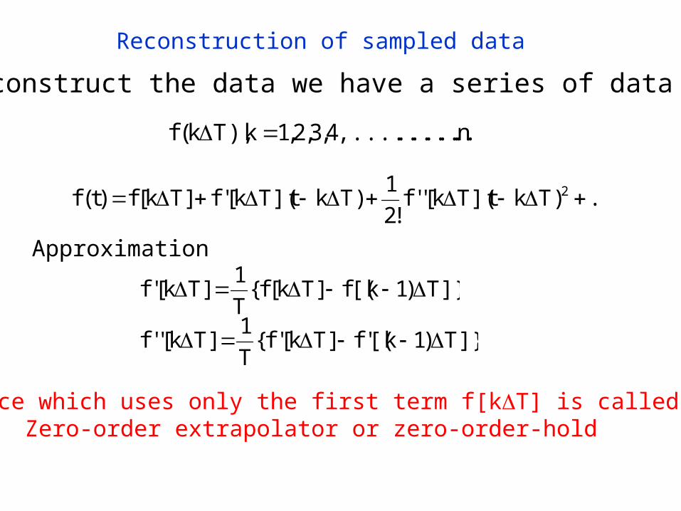
Reconstruction of sampled data
To reconstruct the data we have a series of data
n...........,.........4,3,2,1k),Tk(f
..)Tkt](Tk[''f!2
1)Tkt](Tk['f]Tk[f)t(f 2
Approximation
]}T)1k[(f]Tk[f{T
1]Tk['f
]}T)1k[('f]Tk['f{T
1]Tk[''f
A device which uses only the first term f[kT] is called aZero-order extrapolator or zero-order-hold
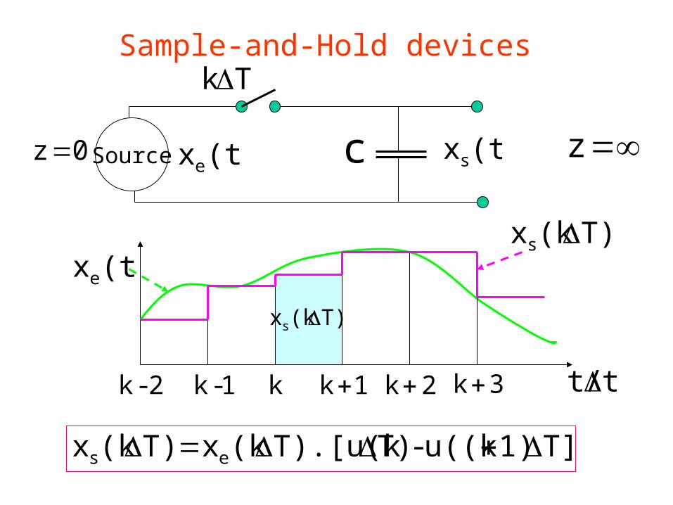
Sample-and-Hold devicesTk
Source c (t)xs z0z (t)xe
T]1)u((k-T)T).[u(k(kxT)(kx es
k1-k2-k 1k 2k 3k
(t)xe
tt/
T)(kxs
T)(kxs
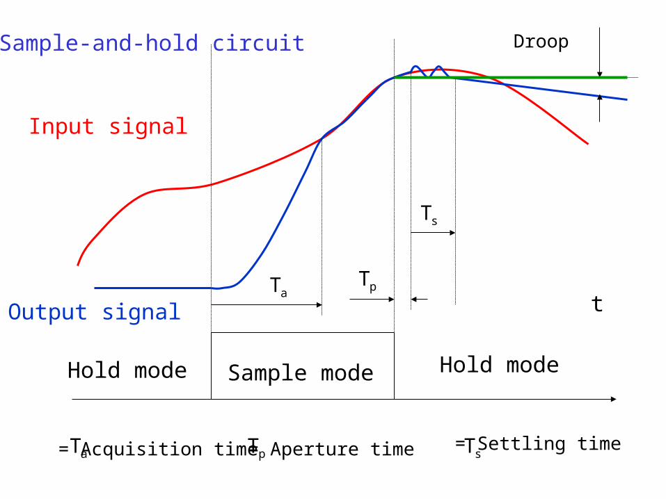
t
Sample modeHold mode Hold mode
Input signal
Output signalaT
Droop
pT
sT
= Acquisition time = Aperture time = Settling timeaT pT sT
Sample-and-hold circuit
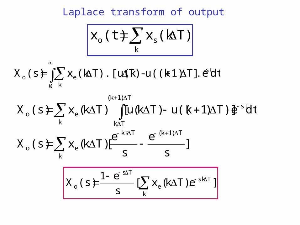
T)(kx(t)xk
so
dt.eT]1)u((k-T)T).[u(k(kx(s)X st-
0 keo
k
T)1k(
Tk
steo dte)]T)1k((u)Tk(u[)Tk(x(s)X
]s
e
s
e[)Tk(x(s)X
T)1k(Tks
keo
]e.)Tk(x[s
e1(s)X Tsk
ke
Ts
o
Laplace transform of output
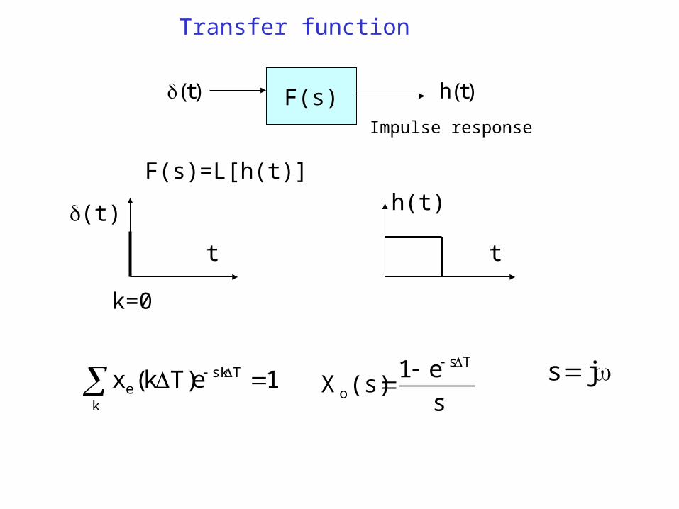
Transfer function
F(s))t( )t(h
Impulse response
F(s)=L[h(t)]
js1e)Tk(x Tsk
ke
s
e1(s)X
Ts
o
h(t)
t
(t)
t
k=0
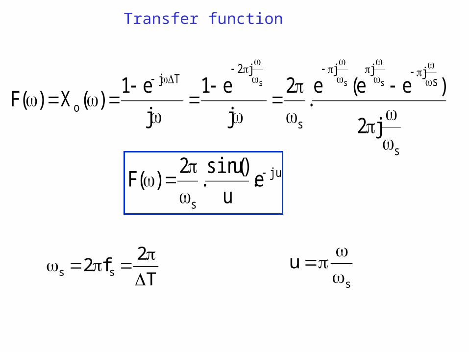
s
sjjj
s
j2Tj
o
j2
)ee(e.
2
j
e1
j
e1)(X)(F
sss
T
2f2 ss
ju
s
e.u
)usin(.
2)(F
s
u
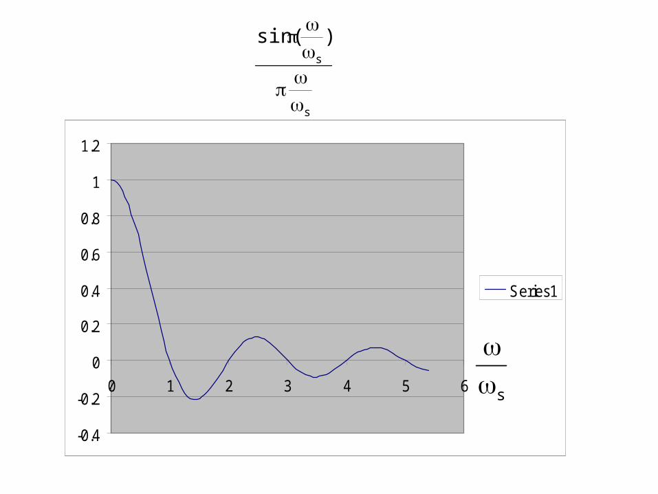
Transfer function
-0.4
-0.2
0
0.2
0.4
0.6
0.8
1
1.2
0 1 2 3 4 5 6
Series1
s
s
s
)sin(
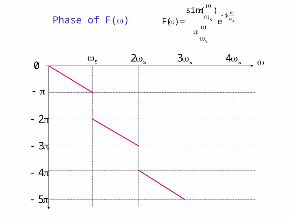
Phase of F() s
j
s
s e
)sin(
)(F
s s2 s3 s40
2
3
4
5
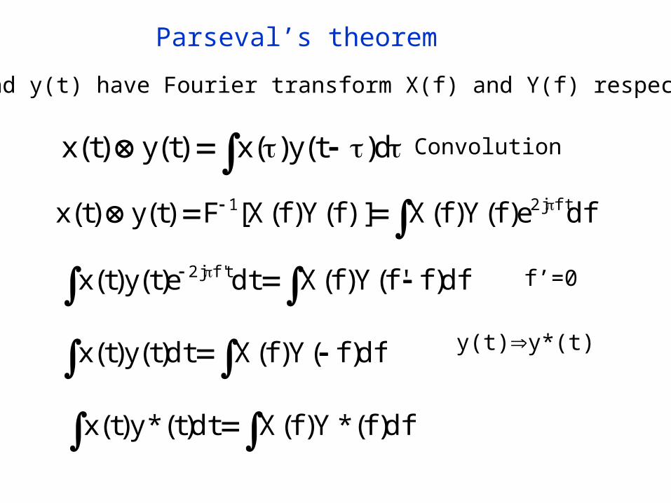
Parseval’s theorem
x(t) and y(t) have Fourier transform X(f) and Y(f) respectively
d)t(y)(x)t(y)t(x Convolution
dfe)f(Y)f(X)]f(Y)f(X[F)t(y)t(x ftj21
df)f'f(Y)f(Xdte)t(y)t(x t'fj2 f’=0
df)f(Y)f(Xdt)t(y)t(x y(t)y*(t)
df)f(*Y)f(Xdt)t(*y)t(x
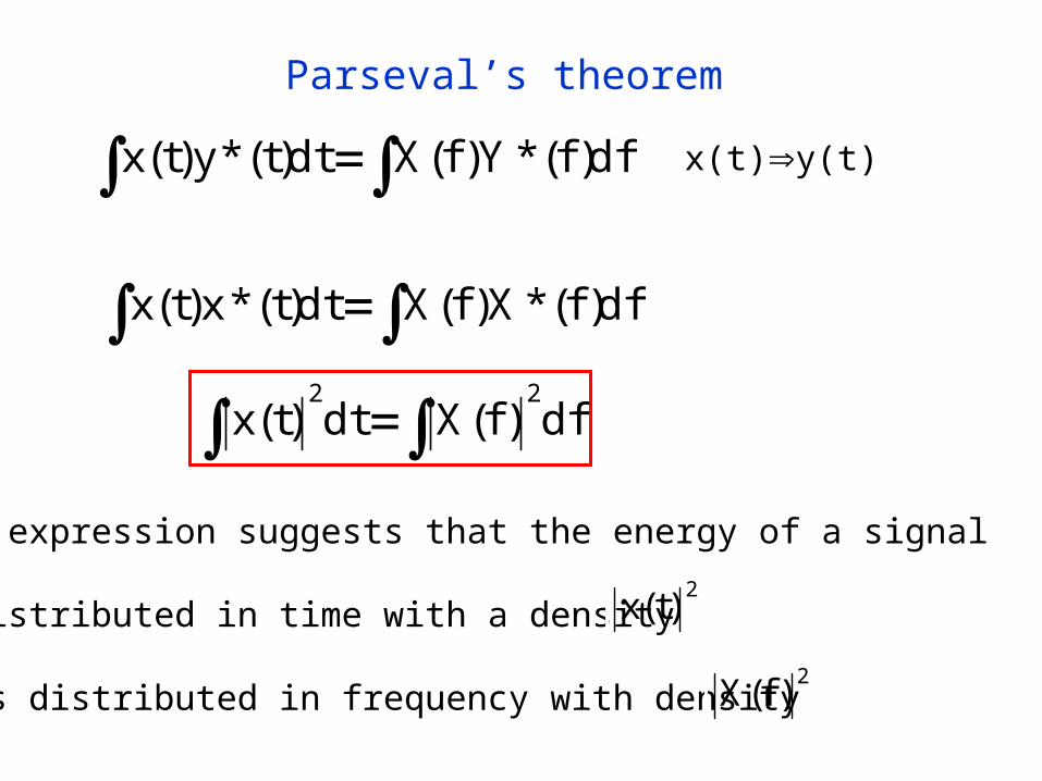
Parseval’s theorem
df)f(*Y)f(Xdt)t(*y)t(x x(t)y(t)
df)f(*X)f(Xdt)t(*x)t(x
df)f(Xdt)t(x22
This expression suggests that the energy of a signal
Is distributed in time with a density
Or is distributed in frequency with density
2)t(x
2)f(X