ANALYSES Are Slovak Retail Gasoline and Diesel Price

ANALYSES

138

Are Slovak Retail Gasoline and Diesel Price Reactions on Crude Oil Changes Asymmetric?

1 University of Economics in Bratislava, Dolnozemská 1/b, 852 35 Bratislava, Slovakia. Corresponding author: e-mail: [email protected], phone: (+421)267295822.

2 A partial output of our study has been also published in Szomolányi et al. (2019).

Abstract

The paper explains why the Slovak retail gasoline and diesel prices rise more rapidly when the price of crude oil increases and fall slowly when the price of crude oil decreases. The weekly data of Slovak retail gasoline and diesel prices and European Brent oil prices since the first week of 2009 till the second week of 2019 are used. The error correction model with irreversible behaviour of explanatory variables is specified to test asymmetric response of retail gasoline and diesel prices on changes in crude oil prices. By our assumption of linked gasoline and diesel markets, we also adopt a common co-integration relationship. Consequently, the vector error correction model is included in the analysis. An expected asymmetry in the retail fuel price reactions on crude oil changes is rejected. Our results may be informative for the future research in Slovak business cycles and in market structure of retail gasoline and diesel sellers.

Keywords

Gasoline and diesel retail prices, crude oil prices, irreversible model, co-integration,

asymmetries between the price of crude oil and the retail fuel

JEL code

C22, Q31

INTRODUCTIONThis paper answers a question if the Slovak retail gasoline and diesel prices rise more rapidly when the price of crude oil increases and fall slowly when the price of crude oil decreases.2

Our motivation comes from following macroeconomic and microeconomic issues. Macroeconomic models of business cycles often lead to the assumption that firms adjust prices infrequently. In recent years, the increasing popularity of the New Keynesian research program has bolstered a line of inquiry into various empirical features of price stickiness. One possible explanation for price rigidity is the asymmetric reaction of output prices to input prices in production. Typical example is that, the fuel prices react more rapidly, when the crude oil price increases and fall slowly when the crude oil

Karol Szomolányi 1 | University of Economics in Bratislava, Bratislava, SlovakiaMartin Lukáčik | University of Economics in Bratislava, Bratislava, SlovakiaAdriana Lukáčiková | University of Economics in Bratislava, Bratislava, Slovakia

2020

139

100 (2)STATISTIKA

price decreases (Douglas and Herrera, 2010). New Keynesian dynamic stochastic general equilibrium models have been increasingly used in the analysis of Slovak business cycles. In order to form the New Keynesian model correctly, we consider being it necessary to understand the origin of price rigidities. The price asymmetry can be caused by an imperfect market structure or an adjustment costs in production or inventory. Our result may be informative in research areas mentioned above.

A traditional approach to test asymmetric response of retail gasoline and diesel prices on changes in crude oil prices is the use of error correction models (ECM) and vector error correction models (VECM); e.g. Radchenko (2005), Grasso and Manera (2007), Honarvar (2009), Liu et al. (2010). In our paper we use this approach to test asymmetry between the price of BRENT crude oil and the Slovak retail gasoline and diesel price in the period 2009–2019. Our analysis uses weekly data. In addition to the commonly used single-equation error correction approach, it complements the multiple-equation error correction approach, as we assume that the gasoline and diesel markets in Slovakia are in the long-run interconnected and interact with each other. Therefore, we expect two co-integration relationships between the crude oil price and the retail fuel price for gasoline and for diesel. We confirm this assumption in our analysis. On the other hand, the asymmetric reactions of gasoline and diesel retail prices on changes in crude oil price are not supported in our analysis.

After the introduction in which we present motivation and brief methodology comment, the literature review follows. Section 2 presents the adopted methodology for both single-equation and multiple-equation approach. Section 3 describes the data set and it points to one significant tax change. Section 4 illustrates the results of our empirical analysis. The final section summarizes and provides conclusion.

1 LITERATURE REVIEWThere is a common belief that the retail gasoline prices rise more rapidly when the price of crude oil increases and fall slowly when the price of crude oil decreases. Borenstein et al. (1997) find the evidence of short-run asymmetry between the price of crude oil and the retail gasoline. Chen et al. (2005) find evidence of long-run and short-run asymmetries. Grasso and Manera (2007) find mixed evidence of long-run asymmetries following a crude oil shock for five European countries. Other studies indicating asymmetries between the price of crude oil and the retail gasoline are those by Radchenko (2005), Honarvar (2009), Meyler (2009), Liu et al. (2010), Rahman (2016), Sun et al. (2018), Bagnai et al. (2018), Bumpass et al. (2019).

Several explanations of the asymmetry have been proposed and tested. A short review is provided by Brown and Yücel (2000) and also Radchenko (2005). Borenstein et al. (1997) suggest three possible explanations for the asymmetric response of gasoline prices: (i) the oligopolistic coordination theory, (ii) the production and inventory cost of adjustment, and (iii) the search theory.

When the crude oil price rises in an industry with a few dominant firms, each firm is quick to raise its selling price because it wishes to signal its competitors that it is adhering to the tacit agreement by not cutting its margin. When the crude oil price falls, each firm is slow to lower its selling price because doing so runs the risk of sending a signal to its competitors that it is cutting its margin and no longer adhering to the tacit agreement.

Borenstein and Shepard (2002) argue that the costs of adjustment of production and inventory cause the asymmetric response of gasoline prices. Since the adjusting levels of production and inventory is costly, firms spread the adjustment over time. A reduction in the price of crude oil, for example, will imply some long-run increase in the supply of gasoline. But if there are adjustment costs that increase with the absolute size of adjustment per period, firms will spread the adjustment over time, gradually achieving the full quantity increase implied by the decline in cost.

ANALYSES

140

According to the search theory, an increase in the retail price of gasoline raises incentives to search for a lower priced retail outlet, while a decrease in the price lowers the incentive to search. Different search rules of consumers influence the elasticity of a retailer’s demand and this leads to the asymmetric response of gasoline prices.

A broad descriptive approach was taken by Peltzman (2000). The author examines how the measures of imperfect competition, inventory cost, inflation-related asymmetric menu costs, and input price volatility influence the degree of asymmetry. In this study, Peltzman finds a negative correlation between the degree of asymmetry and input price volatility, but he finds no relationship between the degree of asymmetry and proxies for market power, inventory cost, and asymmetric menu costs.

While there is a lot of evidence suggesting asymmetry between the price of oil and retail gasoline, on the other hand, there are many papers with opposite results. Applying a threshold regression model, Godby et al. (2000) are unable to find evidence of the asymmetric adjustment in the Canadian gasoline market. Peltzman (2000) shows that the problem of an asymmetric response of output prices to changes in input prices is not specific to the gasoline market.

Bachmeier and Griffin (2003) report no evidence of asymmetry in the U.S. wholesale gasoline market for daily spot gasoline and crude oil price data, over the period 1985–1998. Bettendorf et al. (2003) study the retail price adjustment in the Dutch gasoline market. These authors argue that conclusions on the asymmetry are dependent on the choice of the day when the prices are observed.

Venditti (2010) also reports no systematic evidence of asymmetry for the U.S. as well as Euro areas over 1999–2009, using nonlinear impulse response functions with asymmetric price adjustment, as opposed to the traditional linear impulse response functions used in previous studies.

In recent papers Bagnai et al. (2018) indicate that the relationship between the U.S. prices of gasoline and crude oil has undergone a single structural break in the late 2008, and that after the break extreme observations have a non-negligible role in shaping asymmetry. Bumpass et al. (2019) fail to reject long-run symmetry at each stage of the retail gasoline supply chain in the U.S. market.

2 METHODOLOGYWe are interested in the question as to whether a positive unit change in the oil price has an identical influence on the fuel price as a negative unit change. The error correction model with irreversible behaviour of explanatory variables is considered to be the basic tool for the analysis of the asymmetric price reaction of fuel. The reason for this is clear: if non-stationary price variables are used as the first differences in this model, it is thus easy to separate positive and negative values in the explanatory variable.

A non-stationarity of variables is tested by unit root tests. We prefer the augmented Dickey-Fuller (ADF) test (Dickey and Fuller, 1981). The conventional unit root tests are biased when the data are trend stationary with a structural break. To avoid this problem, we also test variables using the Perron breakpoint unit root procedure (Perron, 1988).

2.1 The single-equation co-integration approachThe single-equation error correction model is essentially an auto-regressive distributed lag model with rearranged terms. We can show it by the auto-regressive distributed lag model of order one with three variables (ARDL(1,1,1)):

0 1 1 0 1 1 0 1 1t t t t t t ty y x x z z uβ β γ γ δ δ− − −= + + + + + + , (1)

where yt is regressand – an average weekly price of gasoline or diesel in time t; xt is the key regressor – an average weekly price of oil in time t; zt is another relevant regressor in time t (a diesel price

2020

141

100 (2)STATISTIKA

in the gasoline equation or a gasoline price in the diesel equation for example); ut is a stochastic term in time t and β0, β1, γ0, γ1, δ0 and δ1 are unknown parameters of this regression model.

We can rewrite model (1) as the error correction (ECM) model (Engle and Granger, 1987):

( ) ( ) ( )0 1 0 1

0 0 0 1 1 1 11 1

11 1t t t t t t ty x z y x z uγ γ δ δ

β γ δ ββ β− − −

+ + ∆ = + ∆ + ∆ + − − − + − −

, (2)

which contains the original (one period lagged) variables in the levels and their first differences. This allows us to explore both the long-run equilibrium relationship and its adjustment along with the short-run dynamics. If a positive unit change of the regressor has an identical influence on the regressand as a negative unit change, we do not have to distinguish between them and we can estimate the overall response with one parameter for one regressor, as in the reversible model. But this is precisely a restriction. If this restriction is not valid, the estimation results can be improved by specifying increases (∆+xt) and decreases (∆–xt) of the explanatory variable as separate variables and also by separating the positive and non-positive deviations from the long-run equilibrium relationship.

The asymmetric form of this irreversible error correction (A-ECM) model (Granger and Lee, 1989) is:

( ) ( )0 0 0 0 1 1 1 10 0t t t t t t t t ty x x z e D e e D e uβ γ γ δ λ λ+ + − − + −− − − −∆ = + ∆ + ∆ + ∆ + × > + × ≤ +

, (3)

where: ( ) ( )0 1 0 1

1 1 1 11 11 1t t t te y x z

γ γ δ δβ β− − − −

+ += − −

− − is one period lagged deviation from the long-run

equilibrium relationship; D(et-1 > 0) is a dummy variable that equals 1 if et-1 > 0 and equals 0 otherwise; D(et-1 ≤ 0) is a dummy variable that equals 1 if et-1 ≤ 0 and equals 0 otherwise; λ+ and λ– are the corresponding adjustment parameters, β0, γ0

+, γ0– and δ0 are also parameters of this regression.

Model (2) is obtained from model (3) using restrictions λ+ = λ– and γ0+ = γ0

–. This linear hypothesis in the linear model can be tested by the F test. In cases where model (1) has a more extensive dynamic structure, both models (2) and (3) will be also more extensive and the test hypothesis will additionally include parameter comparisons for further lags. Models (2) and (3) are some of the simplest types of error correction models, because their long-run equilibrium relationship does not contain any deterministic terms. When searching for the most appropriate specification of the model, it is necessary to analyse different versions of deterministic components as a constant and trend in both long-run relationship and short-run dynamic part of the equation. This brings us to the well-known five cases of the deterministic part of the model: no constant and no trend, restricted constant and no trend, unrestricted constant and no trend, unrestricted constant and restricted trend, unrestricted constant and unrestricted trend; among these we have to decide.

The single equation error correction models are usually estimated by means of a two-step Engle-Granger procedure (Engle and Granger, 1987) and the co-integration of variables is confirmed by an ADF test of residuals from the first step with the MacKinnon (1991) critical values adjusted for the number of variables. The estimates from the static long-run equation (the first step of the Engle-Granger procedure), although consistent, can be substantially biased in small samples, partly due to serial correlation in the residuals. In the first step of Engle-Granger procedure we use fully modified ordinary least squares (FMOLS) method proposed by Phillips and Hansen (1990). The FMOLS estimator employs a semi-parametric correction to eliminate problems caused by the long run correlation between the co-integrating equation and stochastic regressors’ innovations. The FMOLS estimator is asymptotically unbiased and is efficient as other used methods e.g. dynamic ordinary least squares method.

ANALYSES

142

The bias can be reduced by allowing for some dynamics in the long-run equation. In the first stage of Engle-Granger procedure we can estimate an autoregressive distributed lag (ARDL) model and solve for the long-run equation. Its residuals are a measure of disequilibrium and a test of co-integration is a test for the stationarity residuals. As an alternative to the two-step Engle and Granger procedure with the static long-run equation, the ECM model can be estimated just using the residuals from this ARDL model.

The co-integration of variables can be also verified by bounds testing. Pesaran et al. (2001) propose a test for co-integration that is robust with regard to the fact as to whether variables of interest are stationary or integrated of order one, or mutually co-integrated. They suggest a bounds test for co-integration as a test on parameter significance in the co-integrating relationship of the conditional error correction model. Once the test statistic is computed, it is compared to two asymptotic critical values corresponding to two opposite cases: in the first case, all variables are purely stationary, in the second one they are purely integrated of order one. When the test statistic is below the lower critical value, one fails to reject the null and concludes that co-integration is not possible. In contrast, when the test statistic is above the upper critical value, one rejects the null and concludes that co-integration is indeed possible. In either of these two cases, knowledge of the co-integrating rank is not necessary. Alternatively, if the test statistic is between the lower and upper critical values, testing is inconclusive, and knowledge of the co-integrating rank is required to proceed.

After the validation of co-integration, we form the asymmetric ECM and test the appropriate restrictions. In the asymmetric ECM, we do not re-estimate the co-integration relationship which is included in the variable representing the deviation from equilibrium.

2.2 The multiple-equation co-integration approachWe expect that there are co-integrating relationships between the crude oil price and one each for the retail fuel prices, for gasoline and for diesel, either individually or jointly; therefore, we are looking for a long-term equilibrium relationship between the price of oil and the retail price of fuel with the help of the vector error correction model (VECM).

Similarly, as the single-equation error correction model is an auto-regressive model, so the vector error correction model is a vector auto-regressive model. We can show it by the vector auto-regressive model of order two:

t t 1 t-1 2 t-2 ty = ΦD +Π y +Π y +u , (4)

where: yt is the vector of variables (gasoline price, diesel price and oil price) in time t; Dt is the matrix of deterministic terms (constant, trend, …) in time t; ut is the vector of stochastic terms in time t and Φ, Π1 and Π2 are the matrices of unknown parameters of this model.

We can rewrite model (4) as the vector error correction (VECM) model of order one:

1

T∆ + ∆t t t-1 t-1 ty = ΦD +αβ y Φ y +u , (5)

where: ( ) 1 and T − −1 2 2αβ = Π +Π I Φ = Π . Model (5) contains the original (one period lagged) variables in the levels and their first differences, and allows us to explore both the long-run equilibrium relationship and its adjustment along with short-run dynamics. Matrix β is called a co-integration matrix with co-integration vectors as columns and matrix α is called a loading matrix. Again, it is necessary to analyse different versions of deterministic components ΦDt corresponding to five cases mentioned in part 2.1.

2020

143

100 (2)STATISTIKA

The asymmetric form of this irreversible vector error correction (A-VECM) model is:

( ) ( )T T T TD D− − − = × > × ≤ + + + + +

t t t-1 t-1 t-1 t-1 1 t-1 1 t-1 tΔy ΦD +α β y β y 0 +α β y β y 0 +Φ Δ y Φ Δ y u , (6)

where: βTyt-1 is the vector of one period lagged deviations from the long-run equilibrium relationships; D(βTyt-1 > 0) is the vector of a dummy variable; its element equals 1 if corresponding element of βTyt–1 is positive and equals 0 otherwise; similarly D(βTyt–1 ≤ 0) is the vector of a dummy variable; its element equals 1 if corresponding element of βTyt-1 is not positive and equals 0 otherwise; α+ and α– are the loading matrices of corresponding adjustment parameters and Φ1

+ and Φ1– are also matrices with

some pairs of the asymmetric parameters of this model. The multiplication operation in square brackets of model (6) does not represent the matrix product, but the product of elements in the same positions in corresponding vectors. Model (5) is obtained from model (6) using restrictions Φ1

+ = Φ1– and α+ = α–.

The test of co-integration in VECM is realized by Johansen’s procedure (Johansen, 1988, 1991) by the lambda trace statistics depending on the specification of the deterministic components of model (5). After the validation of co-integration, we form the asymmetric VECM and test the appropriate restrictions. In the asymmetric VECM, we do not re-estimate co-integration relationships, which are included in the variables representing the deviations from the equilibrium.

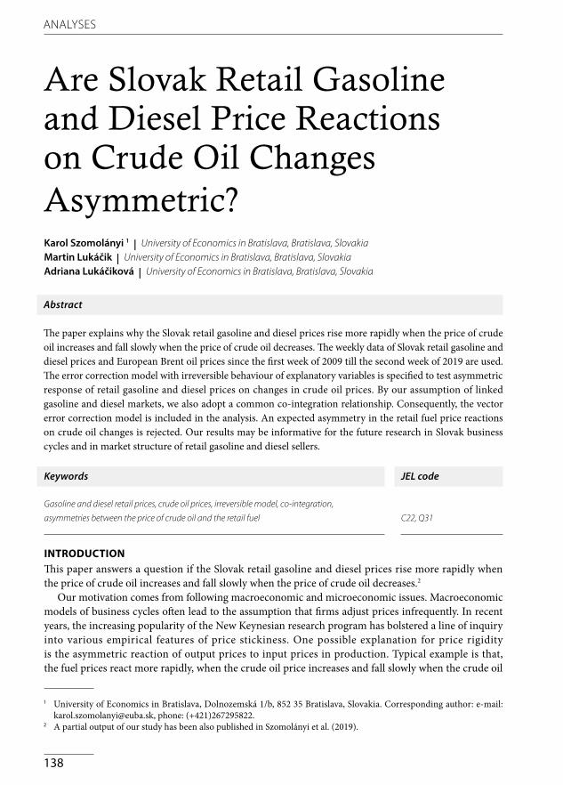
3 DATA AND TAX LEGISLATION Data of retail gasoline and diesel prices on Slovak market are gathered from the Statistical Office of the Slovak Republic. The spot prices for crude oil and petroleum products are gathered from the U.S. Energy Information Administration – the agency responsible for collecting, analysing, and disseminating energy information. Since we only have the weekly retail gasoline and diesel prices data, we can only use the weekly Europe Brent Spot Price FOB Dollars per Barrel for the analysis.

The weekly retail gasoline and diesel prices data are in euros, so we need to recalculate the crude oil prices from dollars to euros. We converted the daily oil prices in dollars by the euro exchange rate in dollars and then aggregated them into weekly averages. The daily reference exchange rate data series are gathered from the European Central Bank. All data pertains to the period from the first week

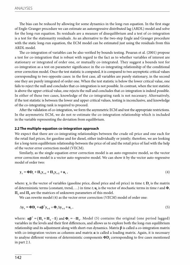
Figure 1 The Weekly Crude Oil Price and the Retail Gasoline Price (€)

Source: The Statistical Office of the Slovak Republic and the U.S. Energy Information Administration

0.000

0.200

0.400

0.600

0.800

1.000

1.200

1.400

1.600

1.800

0

20

40

60

80

100

120

2009 2010 2011 2012 2013 2014 2015 2016 2017 2018 2019

Crude OilGasoline

EUR

per l

itre

EUR

per b

arre

l

Time

ANALYSES

144

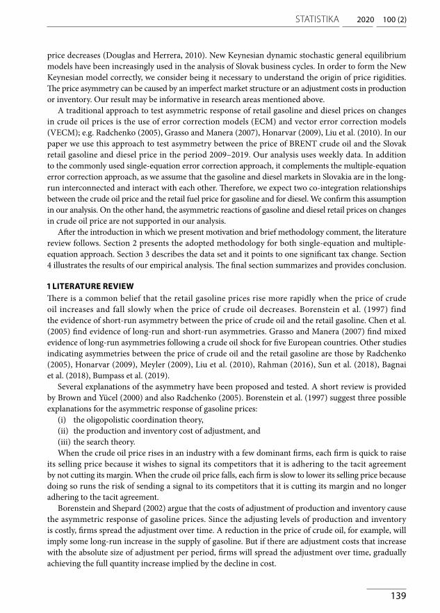
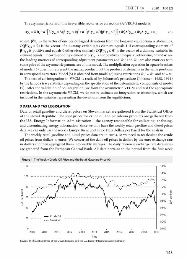
of 2009 till the second week of 2019, so we have 524 observations available. The graph of weekly crude oil price and the retail gasoline price is in Figure 1 and graph of weekly crude oil price and the retail diesel price is in Figure 2.

Liu et al. (2010) outline that taxes and levies make up a significant proportion of retail fuel prices and any changes in government taxes and levies can therefore have a significant impact on retail diesel and gasoline prices. During the period analysed, there was no significant change in consumption taxes, apart from February 2010, when almost a quarter of the consumption taxes on diesel decreased. In other cases, only the classification and categorization of fuels (due to biofuels), without significant intervention in tax rates (no more than 2%), occurred in legislative changes. The impact of the tax change on the consumption tax on diesel can be clearly seen also in the chart of the retail price for diesel. We have highlighted it by shading the graph area in Figure 2.

Figure 2 The Weekly Crude Oil Price and the Retail Diesel Price (€)

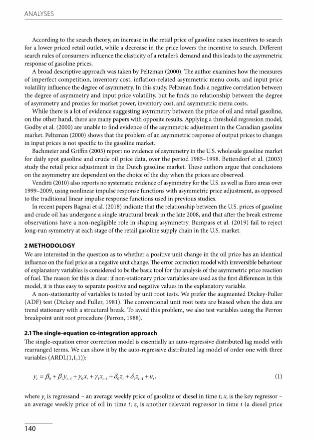
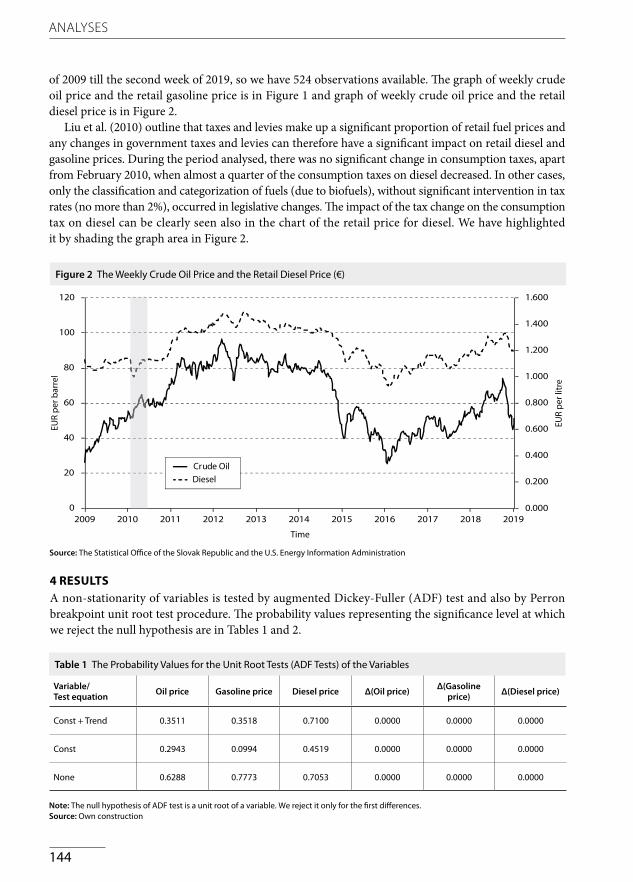
Table 1 The Probability Values for the Unit Root Tests (ADF Tests) of the Variables

Source: The Statistical Office of the Slovak Republic and the U.S. Energy Information Administration

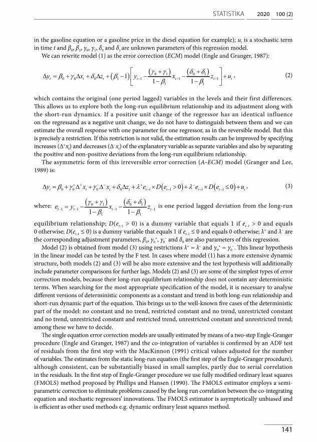
4 RESULTSA non-stationarity of variables is tested by augmented Dickey-Fuller (ADF) test and also by Perron breakpoint unit root test procedure. The probability values representing the significance level at which we reject the null hypothesis are in Tables 1 and 2.

Variable/Test equation Oil price Gasoline price Diesel price Δ(Oil price) Δ(Gasoline

price) Δ(Diesel price)

Const + Trend 0.3511 0.3518 0.7100 0.0000 0.0000 0.0000

Const 0.2943 0.0994 0.4519 0.0000 0.0000 0.0000

None 0.6288 0.7773 0.7053 0.0000 0.0000 0.0000

Note: The null hypothesis of ADF test is a unit root of a variable. We reject it only for the first differences.Source: Own construction

0.000

0.200

0.400

0.600

0.800

1.000

1.200

1.400

1.600

0

20

40

60

80

100

120

2009 2010 2011 2012 2013 2014 2015 2016 2017 2018 2019

Crude OilDiesel

EUR

per b

arre

l

EUR

per l

itre

Time

2020

145

100 (2)STATISTIKA

Variable/Break specification Oil price Gasoline price Diesel price Δ(Oil price) Δ(Gasoline

price) Δ(Diesel price)

Trend + Intercept 0.7013 0.8167 0.9670 <0.01 <0.01 <0.01

Trend 0.8933 0.7179 0.9035 <0.01 <0.01 <0.01

Intercept 0.2242 0.6018 0.7867 <0.01 <0.01 <0.01

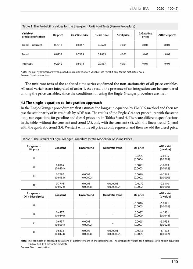
Table 2 The Probability Values for the Breakpoint Unit Root Tests (Perron Procedure)

Note: The null hypothesis of Perron procedure is a unit root of a variable. We reject it only for the first differences.Source: Own construction

The unit root tests of the analysed time series confirmed the non-stationarity of all price variables. All used variables are integrated of order 1. As a result, the presence of co-integration can be considered among the price variables, since the conditions for using the Engle-Granger procedure are met.

4.1 The single-equation co-integration approachIn the Engle-Granger procedure we first estimate the long-run equation by FMOLS method and then we test the stationarity of its residuals by ADF test. The results of the Engle-Granger procedure with the static long-run equations for gasoline and diesel prices are in Tables 3 and 4. There are different specifications in the table: without the constant and trend (A), only with the constant (B), with the linear trend (C) and with the quadratic trend (D). We start with the oil price as only regressor and then we add the diesel price.

Table 3 The Results of Engle-Granger Procedure (Static Model) for Gasoline Prices

Note: The estimates of standard deviations of parameters are in the parentheses. The probability values for τ statistics of long-run equation residual ADF test are in the brackets.

Source: Own construction

Exogenous:Oil price Constant Linear trend Quadratic trend Oil price ADF τ stat

[p-value]

A – – – 0.0205(0.0004)

–2.0835[0.2063]

B 0.8965(0.0201) – – 0.0072

(0.0003)–3.8809[0.0112]

C 0.7797(0.0153)

0.0003(0.00002) – 0.0079

(0.0002)–6.2863[0.0000]

D 0.7716(0.0124)

0.0008(0.00008)

0.000001(0.0000002)

0. 0072(0.0002)

–7.3910[0.0000]

Exogenous:Oil + Diesel price Constant Linear trend Quadratic trend Oil price ADF τ stat

[p-value]

A – – – –0.0016(0.0005)

–5.0121[0.0002]

B 0.4577(0.0840) – – 0.0027

(0.0009)–4.1931[0.0148]

C 0.6537(0.0591)

0.0003(0.00002) – 0.0065

(0.0007)–5.0738[0.0028]

D 0.6333 (0.0474)

0.0008(0.00008)

0.000001(0.0000002)

0. 0056(0.0005)

–6.1232[0.0002]

ANALYSES

146

The results of all models (except the model without the constant and trend and without another regressor) confirm the justification for using co-integration equation for modelling the long run relationships between pairs of prices. Likewise, it seems to be appropriate to include the linear trend into the long run relationships for both prices (we should not use it only in the model for diesel prices with gasoline price as regressor).

All the estimates of static co-integration equations have auto-correlated residuals. We decided to avoid them with the help of dynamic ARDL models. The presented dynamic models were selected from a wide range of models to meet the no residual autocorrelation condition. We can see the results of Engle-Granger procedure with the dynamic long-run equations for the gasoline prices in Table 5 and for the diesel prices in Table 6.

Table 4 The Results of Engle-Granger Procedure (Static Model) for Diesel Prices

Table 5 The Results of Engle-Granger Procedure (Dynamic Model) for Gasoline Prices

Note: The estimates of standard deviations of parameters are in the parentheses. The probability values for τ statistics of long-run equation residual ADF test are in the brackets.


Note: The probability values for τ statistics of ADF test and Ljung-Box Q-statistics are in the brackets.Source: Own construction

Exogenous:Oil price Constant Linear trend Quadratic trend Oil price ADF τ stat

[p-value]

A – – – 0.0189(0.0003)

–2.6352[0.0684]

B 0.7541(0.0151) – – 0.0076

(0.0002)–5.0795[0.0001]

C 0.7090(0.0171)

0.0001(0.00003) – 0.0079

(0.0002)–5.8968[0.0000]

D 0.7063(0.0172)

0.00007(0.0001)

0.0000001(0.0000002)

0. 0079(0.0003)

–5.8929[0.0001]

Exogenous:Oil + Gasoline price Constant Linear trend Quadratic trend Oil price ADF τ stat

[p-value]

A – – – 0.0021(0.0004)

–5.5634[0.0000]

B 0.4688(0.0583) – – 0.0054

(0.0005)–4.7419[0.0024]

C 0.5147(0.0755)

0.00004(0.00004) – 0.0059

(0.0008)–5.6171[0.0003]

D 0.3766(0.0873)

–0.0003(0.0001)

0.0000005(0.0000002)

0. 0049(0.0008)

–5.3886[0.0030]

Exogenous:Oil + Diesel price

ADF τ stat[p-value]

Ljung-Box Q(1)[p-value]




ARDL(2,2,1)no trend

–23.2251[0.0000]

0.7994[0.371]

0.9042[0.636]

0.9110[0.823]

0.9110[0.823]

ARDL(2,2,1)linear trend

–22.9940[0.0000]

0.7681[0.381]

0.8862[0.642]

0.8863[0.829]

0.8863[0.829]

2020

147

100 (2)STATISTIKA

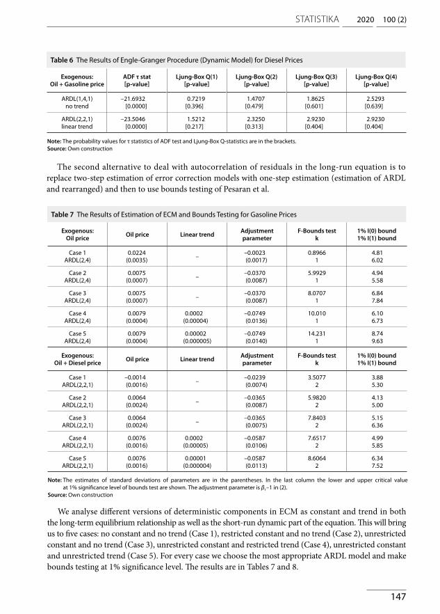
We analyse different versions of deterministic components in ECM as constant and trend in both the long-term equilibrium relationship as well as the short-run dynamic part of the equation. This will bring us to five cases: no constant and no trend (Case 1), restricted constant and no trend (Case 2), unrestricted constant and no trend (Case 3), unrestricted constant and restricted trend (Case 4), unrestricted constant and unrestricted trend (Case 5). For every case we choose the most appropriate ARDL model and make bounds testing at 1% significance level. The results are in Tables 7 and 8.

Exogenous:Oil + Gasoline price

ADF τ stat[p-value]





ARDL(1,4,1)no trend

–21.6932[0.0000]

0.7219[0.396]

1.4707[0.479]

1.8625[0.601]

2.5293[0.639]

ARDL(2,2,1)linear trend

–23.5046[0.0000]

1.5212[0.217]

2.3250[0.313]

2.9230[0.404]

2.9230[0.404]

Table 6 The Results of Engle-Granger Procedure (Dynamic Model) for Diesel Prices

Table 7 The Results of Estimation of ECM and Bounds Testing for Gasoline Prices

Note: The probability values for τ statistics of ADF test and Ljung-Box Q-statistics are in the brackets.Source: Own construction

Note: The estimates of standard deviations of parameters are in the parentheses. In the last column the lower and upper critical value at 1% significance level of bounds test are shown. The adjustment parameter is β1–1 in (2).


The second alternative to deal with autocorrelation of residuals in the long-run equation is to replace two-step estimation of error correction models with one-step estimation (estimation of ARDL and rearranged) and then to use bounds testing of Pesaran et al.

Exogenous:Oil price Oil price Linear trend Adjustment

parameterF-Bounds test

k1% I(0) bound1% I(1) bound

Case 1ARDL(2,4)

0.0224(0.0035) – –0.0023

(0.0017)0.8966

14.816.02

Case 2ARDL(2,4)

0.0075(0.0007) – –0.0370

(0.0087)5.9929

14.945.58

Case 3ARDL(2,4)

0.0075 (0.0007) – –0.0370

(0.0087)8.0707

16.847.84

Case 4ARDL(2,4)

0.0079 (0.0004)

0.0002(0.00004)

–0.0749(0.0136)

10.0101

6.106.73

Case 5ARDL(2,4)

0.0079 (0.0004)

0.00002(0.000005)

–0.0749(0.0140)

14.2311

8.749.63

Exogenous:Oil + Diesel price Oil price Linear trend Adjustment



Case 1ARDL(2,2,1)

–0.0014(0.0016) – –0.0239

(0.0074)3.5077

23.885.30

Case 2ARDL(2,2,1)

0.0064(0.0024) – –0.0365

(0.0087)5.9820

24.135.00

Case 3ARDL(2,2,1)

0.0064 (0.0024) – –0.0365

(0.0075)7.8403

25.156.36

Case 4ARDL(2,2,1)

0.0076 (0.0016)

0.0002(0.00005)

–0.0587(0.0106)

7.65172

4.995.85

Case 5ARDL(2,2,1)

0.0076 (0.0016)

0.00001(0.000004)

–0.0587(0.0113)

8.60642

6.347.52

ANALYSES

148

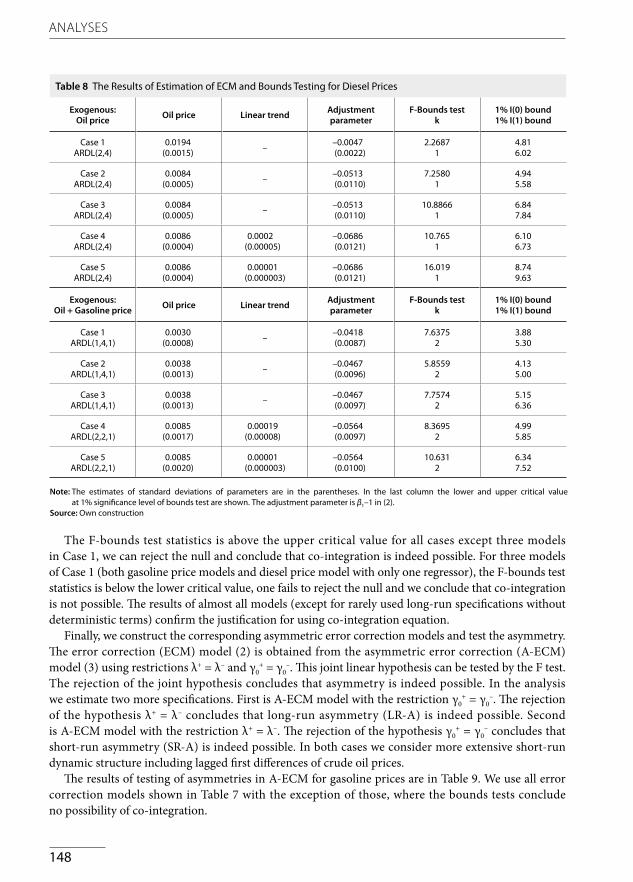
Table 8 The Results of Estimation of ECM and Bounds Testing for Diesel Prices

Note: The estimates of standard deviations of parameters are in the parentheses. In the last column the lower and upper critical value at 1% significance level of bounds test are shown. The adjustment parameter is β1–1 in (2).


Exogenous: Oil price Oil price Linear trend Adjustment



Case 1ARDL(2,4)

0.0194(0.0015) – –0.0047

(0.0022)2.2687

14.816.02

Case 2ARDL(2,4)

0.0084(0.0005) – –0.0513

(0.0110)7.2580

14.945.58

Case 3ARDL(2,4)

0.0084(0.0005) – –0.0513

(0.0110)10.8866

16.847.84

Case 4ARDL(2,4)

0.0086 (0.0004)

0.0002(0.00005)

–0.0686(0.0121)

10.7651

6.106.73

Case 5ARDL(2,4)

0.0086 (0.0004)

0.00001(0.000003)

–0.0686(0.0121)

16.0191

8.749.63

Exogenous:Oil + Gasoline price Oil price Linear trend Adjustment



Case 1ARDL(1,4,1)

0.0030(0.0008) – –0.0418

(0.0087)7.6375

23.885.30

Case 2ARDL(1,4,1)

0.0038(0.0013) – –0.0467

(0.0096)5.8559

24.135.00

Case 3ARDL(1,4,1)

0.0038(0.0013) – –0.0467

(0.0097)7.7574

25.156.36

Case 4ARDL(2,2,1)

0.0085 (0.0017)

0.00019(0.00008)

–0.0564(0.0097)

8.36952

4.995.85

Case 5ARDL(2,2,1)

0.0085 (0.0020)

0.00001(0.000003)

–0.0564(0.0100)

10.6312

6.347.52

The F-bounds test statistics is above the upper critical value for all cases except three models in Case 1, we can reject the null and conclude that co-integration is indeed possible. For three models of Case 1 (both gasoline price models and diesel price model with only one regressor), the F-bounds test statistics is below the lower critical value, one fails to reject the null and we conclude that co-integration is not possible. The results of almost all models (except for rarely used long-run specifications without deterministic terms) confirm the justification for using co-integration equation.

Finally, we construct the corresponding asymmetric error correction models and test the asymmetry. The error correction (ECM) model (2) is obtained from the asymmetric error correction (A-ECM) model (3) using restrictions λ+ = λ– and γ0

+ = γ0–. This joint linear hypothesis can be tested by the F test.

The rejection of the joint hypothesis concludes that asymmetry is indeed possible. In the analysis we estimate two more specifications. First is A-ECM model with the restriction γ0

+ = γ0–. The rejection

of the hypothesis λ+ = λ– concludes that long-run asymmetry (LR-A) is indeed possible. Second is A-ECM model with the restriction λ+ = λ–. The rejection of the hypothesis γ0

+ = γ0– concludes that

short-run asymmetry (SR-A) is indeed possible. In both cases we consider more extensive short-run dynamic structure including lagged first differences of crude oil prices.

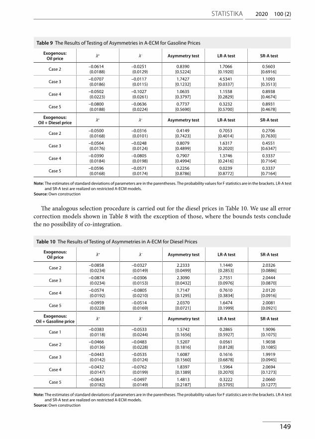
The results of testing of asymmetries in A-ECM for gasoline prices are in Table 9. We use all error correction models shown in Table 7 with the exception of those, where the bounds tests conclude no possibility of co-integration.

2020

149

100 (2)STATISTIKA

Exogenous: Oil price λ+ λ– Asymmetry test LR-A test SR-A test

Case 2 –0.0858(0.0234)

–0.0327(0.0149)

2.2333[0.0499]

1.1440[0.2853]

2.0326[0.0886]

Case 3 –0.0874 (0.0234)

–0.0306 (0.0153)

2.3090[0.0432]

2.7551[0.0976]

2.0444[0.0870]

Case 4 –0.0574 (0.0192)

–0.0805 (0.0210)

1.7147[0.1295]

0.7610[0.3834]

2.0120 [0.0916]

Case 5 –0.0959 (0.0228)

–0.0514 (0.0169)

2.0370[0.0721]

1.6474[0.1999]

2.0081[0.0921]

Exogenous:Oil + Gasoline price λ+ λ– Asymmetry test LR-A test SR-A test

Case 1 –0.0383(0.0118)

–0.0533(0.0244)

1.5742[0.1656]

0.2865[0.5927]

1.9096[0.1075]

Case 2 –0.0466(0.0136)

–0.0483(0.0228)

1.5207[0.1816]

0.0561[0.8128]

1.9038 [0.1085]

Case 3 –0.0443 (0.0142)

–0.0535 (0.0124)

1.6087[0.1560]

0.1616[0.6878]

1.9919 [0.0945]

Case 4 –0.0432 (0.0147)

–0.0762 (0.0199)

1.8397[0.1389]

1.5964[0.2070]

2.0694[0.1273]

Case 5 –0.0643 (0.0182)

–0.0497 (0.0149)

1.4813[0.2187]

0.3222[0.5705]

2.0660[0.1277]

Exogenous: Oil price λ+ λ– Asymmetry test LR-A test SR-A test

Case 2 –0.0614(0.0188)

–0.0251(0.0129)

0.8390[0.5224]

1.7066[0.1920]

0.5603[0.6916]

Case 3 –0.0707 (0.0186)

–0.0117 (0.0115)

1.7427[0.1232]

4.5341[0.0337]

1.1093[0.3513]

Case 4 –0.0502 (0.0223)

–0.1027 (0.0261)

1.0635[0.3797]

1.1558[0.2829]

0.8938 [0.4674]

Case 5 –0.0800 (0.0188)

–0.0636 (0.0224)

0.7737[0.5690]

0.3232[0.5700]

0.8931[0.4678]

Exogenous:Oil + Diesel price λ+ λ– Asymmetry test LR-A test SR-A test

Case 2 –0.0500(0.0168)

–0.0316(0.0101)

0.4149[0.7423]

0.7053[0.4014]

0.2706[0.7630]

Case 3 –0.0564 (0.0176)

–0.0248 (0.0124)

0.8079[0.4899]

1.6317[0.2020]

0.4551[0.6347]

Case 4 –0.0390 (0.0184)

–0.0805 (0.0198)

0.7907[0.4994]

1.3746[0.2416]

0.3337[0.7164]

Case 5 –0.0596 (0.0168)

–0.0571 (0.0174)

0.2256[0.8786]

0.0239[0.8772]

0.3337[0.7164]

Table 9 The Results of Testing of Asymmetries in A-ECM for Gasoline Prices

Table 10 The Results of Testing of Asymmetries in A-ECM for Diesel Prices

Note: The estimates of standard deviations of parameters are in the parentheses. The probability values for F statistics are in the brackets. LR-A test and SR-A test are realized on restricted A-ECM models.


Note: The estimates of standard deviations of parameters are in the parentheses. The probability values for F statistics are in the brackets. LR-A test and SR-A test are realized on restricted A-ECM models.


The analogous selection procedure is carried out for the diesel prices in Table 10. We use all error correction models shown in Table 8 with the exception of those, where the bounds tests conclude the no possibility of co-integration.

ANALYSES

150

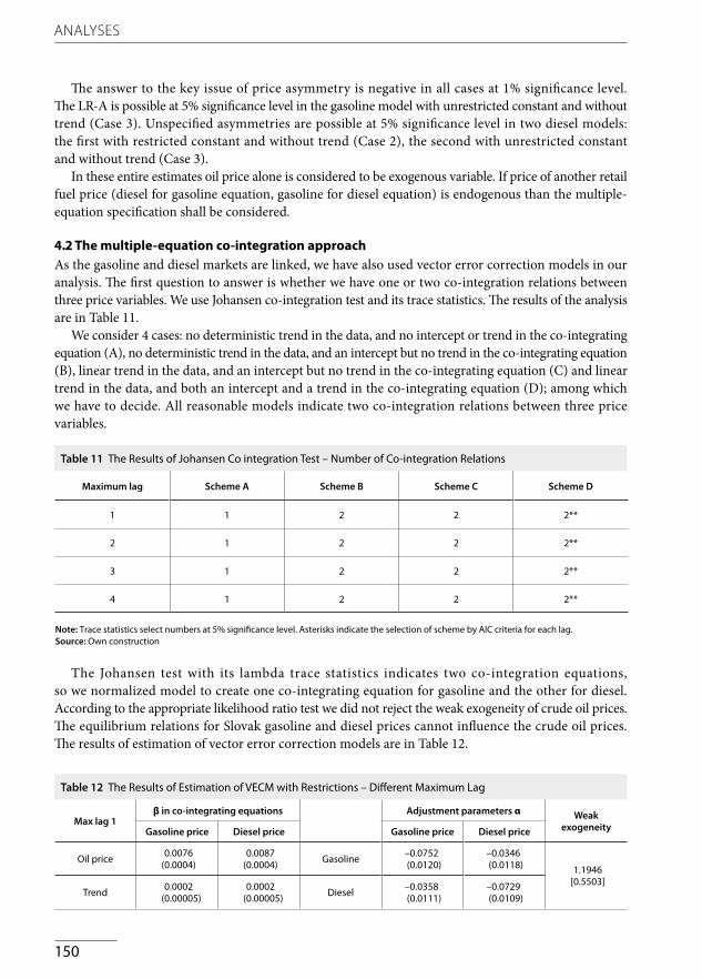
Table 11 The Results of Johansen Co integration Test – Number of Co-integration Relations

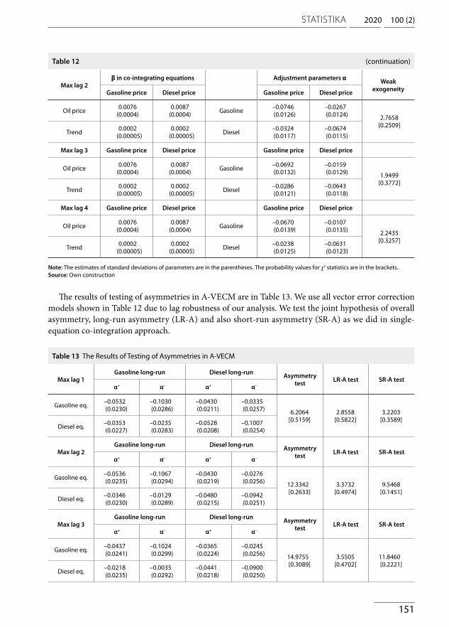
Table 12 The Results of Estimation of VECM with Restrictions – Different Maximum Lag

Note: Trace statistics select numbers at 5% significance level. Asterisks indicate the selection of scheme by AIC criteria for each lag.Source: Own construction

The answer to the key issue of price asymmetry is negative in all cases at 1% significance level. The LR-A is possible at 5% significance level in the gasoline model with unrestricted constant and without trend (Case 3). Unspecified asymmetries are possible at 5% significance level in two diesel models: the first with restricted constant and without trend (Case 2), the second with unrestricted constant and without trend (Case 3).

In these entire estimates oil price alone is considered to be exogenous variable. If price of another retail fuel price (diesel for gasoline equation, gasoline for diesel equation) is endogenous than the multiple-equation specification shall be considered.

4.2 The multiple-equation co-integration approachAs the gasoline and diesel markets are linked, we have also used vector error correction models in our analysis. The first question to answer is whether we have one or two co-integration relations between three price variables. We use Johansen co-integration test and its trace statistics. The results of the analysis are in Table 11.

We consider 4 cases: no deterministic trend in the data, and no intercept or trend in the co-integrating equation (A), no deterministic trend in the data, and an intercept but no trend in the co-integrating equation (B), linear trend in the data, and an intercept but no trend in the co-integrating equation (C) and linear trend in the data, and both an intercept and a trend in the co-integrating equation (D); among which we have to decide. All reasonable models indicate two co-integration relations between three price variables.

Maximum lag Scheme A Scheme B Scheme C Scheme D

1 1 2 2 2**

2 1 2 2 2**

3 1 2 2 2**

4 1 2 2 2**

The Johansen test with its lambda trace statistics indicates two co-integration equations, so we normalized model to create one co-integrating equation for gasoline and the other for diesel. According to the appropriate likelihood ratio test we did not reject the weak exogeneity of crude oil prices. The equilibrium relations for Slovak gasoline and diesel prices cannot influence the crude oil prices. The results of estimation of vector error correction models are in Table 12.

Max lag 1β in co-integrating equations Adjustment parameters α Weak

exogeneityGasoline price Diesel price Gasoline price Diesel price

Oil price 0.0076(0.0004)

0.0087(0.0004) Gasoline –0.0752

(0.0120)–0.0346(0.0118) 1.1946

[0.5503]Trend 0.0002

(0.00005)0.0002

(0.00005) Diesel –0.0358(0.0111)

–0.0729(0.0109)

2020

151

100 (2)STATISTIKA

Max lag 1Gasoline long-run Diesel long-run Asymmetry

test LR-A test SR-A testα+ α– α+ α–

Gasoline eq. –0.0532 (0.0230)

–0.1030 (0.0286)

–0.0430 (0.0211)

–0.0335 (0.0257) 6.2064

[0.5159]2.8558

[0.5822]3.2203

[0.3589]Diesel eq. –0.0353

(0.0227)–0.0235 (0.0283)

–0.0528 (0.0208)

–0.1007 (0.0254)



Gasoline eq. –0.0536 (0.0235)

–0.1067 (0.0294)

–0.0430 (0.0219)

–0.0276 (0.0256) 12.3342

[0.2633]3.3732

[0.4974]9.5468

[0.1451]Diesel eq. –0.0346

(0.0230)–0.0129 (0.0289)

–0.0480 (0.0215)

–0.0942 (0.0251)



Gasoline eq. –0.0437 (0.0241)

–0.1024 (0.0299)

–0.0365 (0.0224)

–0.0245 (0.0256) 14.9755

[0.3089]3.5505

[0.4702]11.8460[0.2221]

Diesel eq. –0.0218 (0.0235)

–0.0035 (0.0292)

–0.0441 (0.0218)

–0.0900 (0.0250)

Max lag 2β in co-integrating equations Adjustment parameters α Weak

exogeneityGasoline price Diesel price Gasoline price Diesel price

Oil price 0.0076(0.0004)

0.0087(0.0004) Gasoline –0.0746

(0.0126)–0.0267(0.0124) 2.7658

[0.2509]Trend 0.0002

(0.00005)0.0002

(0.00005) Diesel –0.0324(0.0117)

–0.0674(0.0115)

Max lag 3 Gasoline price Diesel price Gasoline price Diesel price

Oil price 0.0076(0.0004)

0.0087(0.0004) Gasoline –0.0692

(0.0132)–0.0159(0.0129) 1.9499

[0.3772]Trend 0.0002

(0.00005)0.0002

(0.00005) Diesel –0.0286(0.0121)

–0.0643(0.0118)

Max lag 4 Gasoline price Diesel price Gasoline price Diesel price

Oil price 0.0076(0.0004)

0.0087(0.0004) Gasoline –0.0670

(0.0139)–0.0107(0.0135) 2.2435

[0.3257]Trend 0.0002

(0.00005)0.0002

(0.00005) Diesel –0.0238(0.0125)

–0.0631(0.0123)

Note: The estimates of standard deviations of parameters are in the parentheses. The probability values for χ2 statistics are in the brackets.Source: Own construction

The results of testing of asymmetries in A-VECM are in Table 13. We use all vector error correction models shown in Table 12 due to lag robustness of our analysis. We test the joint hypothesis of overall asymmetry, long-run asymmetry (LR-A) and also short-run asymmetry (SR-A) as we did in single-equation co-integration approach.

Table 12 (continuation)

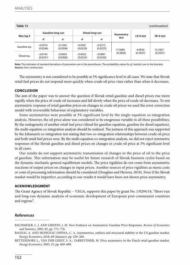
Table 13 The Results of Testing of Asymmetries in A-VECM

ANALYSES

152



Gasoline eq. –0.0374 (0.0246)

–0.1045 (0.0306)

–0.0301 (0.0229)

–0.0215 (0.0255) 17.0085

[0.3850]4.0920

[0.3937]13.1857[0.3557]

Diesel eq. –0.0143 (0.0241)

–0.0024 (0.0300)

–0.0423 (0.0224)

–0.0891 (0.0250)

Note: The estimates of standard deviations of parameters are in the parentheses. The probability values for χ2 statistics are in the brackets.Source: Own construction

The asymmetry is not considered to be possible at 5% significance level in all cases. We state that Slovak retail fuel prices do not respond more quickly when crude oil price rises rather than when it decreases.

CONCLUSIONThe aim of the paper was to answer the question if Slovak retail gasoline and diesel prices rise more rapidly when the price of crude oil increases and fall slowly when the price of crude oil decreases. To test asymmetric response of retail gasoline prices on changes in crude oil prices we used the error correction model with irreversible behaviour of explanatory variables.

Some asymmetries were possible at 5% significant level by the single-equation co-integration analysis. However, the oil price alone was considered to be exogenous variable in all these possibilities. By the endogeneity of another retail fuel price (diesel for gasoline equation, gasoline for diesel equation), the multi-equation co-integration analysis should be realized. The justness of this approach was supported by the Johansen’s co-integration test stating that two co-integration relationships between crude oil price and both retail fuel prices were. By the multi-equation co-integration analysis, we did not reject symmetric responses of the Slovak gasoline and diesel prices on changes in crude oil price at 5% significant level in all cases.

Our results do not support asymmetric transmission of changes in the price of oil to the price of gasoline. This information may be useful for future research of Slovak business cycles based on the dynamic stochastic general equilibrium models. The price rigidities do not come from asymmetric reactions of output prices on changes in input prices. Another sources of price rigidities as menu costs or costs of processing information should be considered (Douglass and Herrera, 2010). Even if the Slovak market would be imperfect, according to our results it would have been not shown price asymmetry.

ACKNOWLEDGMENTThe Grant Agency of Slovak Republic – VEGA, supports this paper by grant No. 1/0294/18, “Short-run and long-run dynamic analysis of economic development of European post-communist countries and regions“.

References

BACHMEIER, L. J. AND GRIFFIN, J. M. New Evidence on Asymmetric Gasoline Price Responses. Review of Economics and Statistics, 2003, 85, pp. 772–776.

BAGNAI, A. AND MONGEAU OSPINA, C. A. Asymmetries, outliers and structural stability in the US gasoline market. Energy Economics, 2018, 69 (January), pp. 250–260.

BETTENDORF, L., VAN DER GEEST, S. A., VARKEVISSER, M. Price asymmetry in the Dutch retail gasoline market. Energy Economics, 2003, 25, pp. 669–689.

Table 13 (continuation)

2020

153

100 (2)STATISTIKA

BORENSTEIN, S., CAMERON, A., GILBERT, R. Do Gasoline Prices Respond Asymmetrically to Crude Oil Price Changes? Quarterly Journal of Economics, 1997, 112, pp. 305–339.

BORENSTEIN, S. AND SHEPARD, A. Sticky Prices, Inventories, and Market Power in Wholesale Gasoline Markets. The RAND Journal of Economics, 2002, 33, pp. 116–139.

BROWN, S. P. A. AND YÜCEL, M. K. Gasoline and crude oil prices: Why the asymmetry? Economic and Financial Policy Review, 2000, Quarter 3, pp. 23–29.

BUMPASS, D., DOUGLAS, C., GINN, V., TUTTLE, M. H. Testing for short and long-run asymmetric responses and structural breaks in the retail gasoline supply chain. Energy Economics, 2019, 83 (September), pp. 311–318.

CHEN, L.-H., FINNEY, M., LAI, K. S. A threshold cointegration analysis of asymmetric price transmission from crude oil to gasoline prices. Economics Letters, 2005, 89, pp. 233–239.

DICKEY, D. A. AND FULLER, W. A. Likelihood Ratio Statistics for Autoregressive Time Series with a Unit Root. Econometrica, 1981, 49, pp. 1057–1072.

DOUGLAS, C. AND HERRERA, A. Why Are Gasoline Prices Sticky? A Test of Alternative Models of Price Adjustment. Journal of Applied Econometrics, 2010, 25, pp. 903–928.

ENGLE, R. F. AND GRANGER, C. W. J. Cointegration and Error Correction: Representation, Estimation and Testing. Econometrica, 1987, 55, pp. 251–276.

GODBY, R., LINTNER, A. M., STENGOS, T., WANDSCHNEIDER, B. Testing for asymmetric pricing in the Canadian retail gasoline market. Energy Economics, 2000, 22, 349–368.

GRANGER, C. W. J. AND LEE, T. H. Investigation of Production, Sales and Inventory Relationships Using Multicointegration and Non-symmetric Error Correction Models. Journal of Applied Econometrics, 1989, 4, Issue S1, pp. 145–159.

GRASSO, M. AND MANERA, M. Asymmetric error correction models for the oil-gasoline price relationship. Energy Policy, 2007, 35, pp. 156–177.

HONARVAR, A. Asymmetry in Retail Gasoline and Crude Oil Price Movements in the United States: an Application of Hidden Cointegration Technique. Energy Economics, 2009, 31, pp. 395–402.

JOHANSEN, S. Statistical Analysis of Cointegration Vectors. Journal of Economic Dynamics and Control, 1988, 12, pp. 231–254.JOHANSEN, S. Estimation and Hypothesis Testing of Cointegration Vectors in Gaussian Vector Autoregressive Models.

Econometrica, 1991, 59, pp. 1551–1580.LIU, M., MARGARITIS, D., TOURANI-RAD, A. Is there an Asymmetry in the Response of Diesel and Petrol Prices

to Crude Oil Price Changes? Evidence from New Zealand. Energy Economics, 2010, 32, pp. 926–932.LJUNG, G. M. AND BOX, G. E. P. On a Measure of Lack of Fit in Time Series Models. Biometrika, 1978, 65, pp. 297–303.MACKINNON, J. G. Critical Values for Cointegration Tests. In: ENGLE, R. F. AND GRANGER, C. W. J. eds. Long-run

Economic Relationships: Readings in Cointegration, Oxford: Oxford University Press, 1991.MEYLER, A. The pass through of oil prices into consumer liquid fuels prices in an environment of high and volatile oil

prices. Energy Economics, 2009, 31, pp. 867–881.PELTZMAN, S. Prices Rise Faster than They Fall. Journal of Political Economy, 2000, 108, pp. 466–502.PERRON, P. The Great Crash, the Oil Price Shock, and the Unit Root Hypothesis. Econometrica, 1989, 57, pp. 1361–1401.PESARAN, M. H., SHIN, Y., SMITH, R. J. Bounds Testing Approaches to the Analysis of Level Relationships. Journal

of Applied Econometrics, 2001, 16, pp. 289–326.PHILLIPS, P. C. B. AND HANSEN, B. E. Statistical Inference in Instrumental Variables Regression with I (1) Processes.

The Review of Economic Studies, 1990, 57, pp. 99–125.RADCHENKO, S. Oil Price Volatility and the Asymmetric Response of Gasoline Prices to Oil Price Increases and Decreases.

Energy Economics, 2005, 27, pp. 708–730.RAHMAN, S. Another Perspective on Gasoline Price Responses to Crude Oil Price Changes. Energy Economics, 2016, 55,

pp. 10–18.SUN, Y., ZHANG, X., HONG, Y., WANG, S. Asymmetric pass-through of oil prices to gasoline prices with interval time

series modelling. Energy Economics, 2018, 78 (February), pp. 165–173.SZOMOLÁNYI, K., LUKÁČIK, M., LUKÁČIKOVÁ, A. Analysis of Asymmetry in Slovak Gasoline and Diesel Retail Market.

In: MILKOVIĆ, M. S. et al. eds. Proceedings of the ENTRENOVA – ENTerprise REsearch InNOVAtion Conference, Rovinj, Croatia, 12–14 September 2019, IRENET – Society for Advancing Innovation and Research in Economy, Zagreb, pp. 359–366.

VENDITTI, F. Down the Non-Linear Road from Oil to Consumer Energy Prices: Not Much Asymmetry Along the Way. Bank of Italy, Economic Research Department, Temi di discussion, Economic working papers, 2010.

Documents

ANALYSES Are Slovak Retail Gasoline and Diesel Price