Analysis and Approximation ofa Fractional Differential

Equation

Marcus Webb

Supervisors:

Prof. Endre Suli

Dr David Kay

Part C Mathematics Dissertation

University of OxfordHilary Term, 2012

Abstract

A differential equation is fractional if it involves an operator that can be considered to

be between a (k − 1)th and kth order differential operator, for some positive integer k,

and it is said to be of fractional-order if this operator is the highest order operator in the

equation. The diffusion equation is of order 2, because its highest order operator is the

Laplacian, a 2nd order differential operator, but we can consider an analogous equation

of order 2s, where s ∈ (0, 1), involving the so-called fractional Laplacian operator. Such

fractional-order equations appear in a surprising number of real world models. For

example, a diffusion model used for cardiac tissue is what is known as anomalous, or

non-Fickian, because the diffusion does not satisfy Fick’s law of diffusion and is not

modelled accurately by the diffusion equation, but actually by a differential equation

of fractional order. The diffusion is also anisotropic (directionally dependent) because

diffusion along fibers happens at a different rate to that across fibers in the tissue; the

mathematical models of are harder to work with. This thesis covers some analysis for

the study of fractional-order advection-diffusion equations relevant to this anisotropic

cardiac tissue model.

The study of fractional-order equations is difficult: Firstly, fractional-order opera-

tors are nonlocal, i.e. the value of a fractional derivative of a function at a point in

the domain depends on values of the function throughout the domain; and secondly,

boundary conditions (traces) do not make sense in fractional Sobolev spaces of order

s ≤ 1/2, so constraints must be defined on a region of non-zero volume. We review

and derive some relevant results on fractional Sobolev spaces, fractional-order operators

and the nonlocal calculus developed by Du, Gunzburger, Lehoucq, Zhou (2011). We

prove well-posedness of a general class of fractional-order elliptic problems and develop

Galerkin approximations, focusing on the derivation of a-priori error bounds.

Preface

This thesis is a fourth year mathematics dissertation worth a whole unit towards the

degree of Master of Mathematics and Computer Science.

The target audience is a fourth year undergraduate at Oxford who has taken the

C5.1a Methods of Functional Analysis for PDEs and C12.2b Finite Element Methods

for PDEs courses. In particular, we assume that the reader is familiar with the following

concepts:

• For k ∈ N, 1 ≤ p ≤ ∞, and open subsets Ω of Rn, basic properties of:

– The Lebesgue spaces Lp(Ω)

– The Sobolev spaces W k,p(Ω), Hk(Ω)

– Continuous function spaces C(Ω), Ck(Ω), C∞(Ω)

– The space of infinitely differentiable functions with compact support C∞0 (Ω)

• The finite element method for second-order elliptic PDEs

• A priori and a posteriori error analysis of these methods

I would like to thank my supervisors David and Endre for their stimulating discus-

sions in our regular meetings, and for their support and encouragement throughout the

last six months.

March 16, 2012

i

Contents

1 Introduction 2

1.1 Introduction . . . . . . . . . . . . . . . . . . . . . . . . . . . . . . . . . . . 2

1.2 Fractional-order models in science and nature . . . . . . . . . . . . . . . . 4

1.3 Fractional-order elliptic problems . . . . . . . . . . . . . . . . . . . . . . . 5

2 Fractional-Order Function Spaces 7

2.1 Smoothness and Regularity . . . . . . . . . . . . . . . . . . . . . . . . . . 7

2.2 Fractional Sobolev spaces . . . . . . . . . . . . . . . . . . . . . . . . . . . 8

2.3 Fourier transform approach . . . . . . . . . . . . . . . . . . . . . . . . . . 9

2.4 Further properties of fractional Sobolev spaces . . . . . . . . . . . . . . . 13

2.5 Traces and fractional Sobolev spaces . . . . . . . . . . . . . . . . . . . . . 14

2.6 The importance of the case s ∈ (0, 12 ) . . . . . . . . . . . . . . . . . . . . . 16

3 Fractional-Order Operators 17

3.1 The Riemann-Liouville fractional derivative . . . . . . . . . . . . . . . . . 17

3.2 Fractional derivatives . . . . . . . . . . . . . . . . . . . . . . . . . . . . . . 19

3.3 Fractional Friedrichs inequality . . . . . . . . . . . . . . . . . . . . . . . . 23

3.4 The fractional Laplacian . . . . . . . . . . . . . . . . . . . . . . . . . . . . 25

4 A Nonlocal Calculus 28

4.1 Notation . . . . . . . . . . . . . . . . . . . . . . . . . . . . . . . . . . . . . 28

4.2 Nonlocal operators . . . . . . . . . . . . . . . . . . . . . . . . . . . . . . . 29

4.3 Properties of the nonlocal calculus . . . . . . . . . . . . . . . . . . . . . . 30

4.4 Inclusion of the classical vector calculus . . . . . . . . . . . . . . . . . . . 32

4.5 Anisotropic fractional Laplacian . . . . . . . . . . . . . . . . . . . . . . . . 33

5 Volume-Constrained Problems 37

5.1 Boundary value problems . . . . . . . . . . . . . . . . . . . . . . . . . . . 37

5.2 Volume-constrained problems . . . . . . . . . . . . . . . . . . . . . . . . . 38

ii

CONTENTS

6 Well-Posedness of Elliptic Problems 40

6.1 Classical statement of the Dirichlet problem . . . . . . . . . . . . . . . . . 40

6.2 Weak formulation . . . . . . . . . . . . . . . . . . . . . . . . . . . . . . . . 41

6.3 Well-posedness of the weak formulation . . . . . . . . . . . . . . . . . . . 42

7 Galerkin Approximation 46

7.1 Approximation of the problem . . . . . . . . . . . . . . . . . . . . . . . . 46

7.2 Convergence in the Hs norm . . . . . . . . . . . . . . . . . . . . . . . . . 47

7.3 Finite elements . . . . . . . . . . . . . . . . . . . . . . . . . . . . . . . . . 47

7.4 Legendre polynomials . . . . . . . . . . . . . . . . . . . . . . . . . . . . . 48

8 Conclusion 49

8.1 Aims of the project . . . . . . . . . . . . . . . . . . . . . . . . . . . . . . . 49

8.2 Further work . . . . . . . . . . . . . . . . . . . . . . . . . . . . . . . . . . 49

A The Fourier Transform 50

B Bilinear Forms on Hilbert Spaces 51

1

Chapter 1

Introduction

1.1 Introduction

A differential equation is fractional if it involves an operator that can be considered to

be between a (k − 1)th and kth order differential operator, for some positive integer k,

and it is said to be a fractional-order differential equation if this operator is the highest

order operator in the equation. What on Earth do we mean by such a vague statement?

Consider Poisson’s equation on an open subset Ω of Rn, with source function f ∈L2(Ω), for a function u ∈ H2(Ω):

−∆u = f. (1.1)

This equation is of order 2 because the Laplacian −∆ = −∑j ∂

2j is a 2nd-order differen-

tial operator. We can consider an analogous equation of order 2s, where s is a positive

real number, involving the so-called fractional Laplacian operator (−∆)s:

(−∆)su = f. (1.2)

How can we define such an operator? What types of functions u can it operate on? The

reader who is familiar with the Fourier transform (Definition A.1) will know that for

functions u ∈ H2(Rn) the Laplacian satisfies

−∆u = F−1[|ξ|2Fu

], (1.3)

so a first guess at a definition for the fractional Laplacian could be:

(−∆)su = F−1[|ξ|2sFu

]. (1.4)

This operator certainly makes sense for u ∈ C∞0 (Rn) (smooth, compactly supported),

but can it be extended to some other function space? Some kind of fractional Sobolev

space H2s(Rn) perhaps (do these spaces even exist)? Does this operator have an explicit

2

CHAPTER 1. INTRODUCTION

form? Can it be generalised to make sense within an open domain Ω ⊂ Rn? We hope

to answer some of these questions.

For a positive integer k, partial derivatives of a function u ∈ Hk(Rn) satisfy:

∂kj u = F−1[(iξj)

kFu], (1.5)

so one could define a partial derivative of order s > 0 for functions in C∞0 (Rn) by:

∂sju = F−1 [(iξj)sFu] . (1.6)

However, with this definition (−∆)s 6=∑j ∂

2sj , because in general (ξ2

1 + · · · + ξ2n)s 6=

ξ2s1 + · · · + ξ2s

n and the Fourier transform is an injective operator. We see further that

if we define a fractional Nabla operator by ∇s = (∂s1 , . . . , ∂sn), then we have (−∆)s 6=

−∇r ·∇t for any r and t; the relationship between the fractional Laplacian and fractional

derivatives of these types are not as simple as in the classical case, in which we have

−∆ = −∇ · ∇.

The classical gradient operator ∇ = (∂1, . . . , ∂n) also has the important property

that it contains all the information required to compute directional derivatives. If m is

a unit vector in Rn, the directional derivative operator in the directionm is simplym·∇.

Checking the difference betweenm·∇s and F−1 [(im · ξ)sFu], we see that this is not the

case for our naıvely defined fractional Nabla gradient ∇s. We need more than just the n

partial derivatives of order s to adequately describe fractional analogues of the gradient

and the divergence. It is for this reason that we do not call fractional-order differential

equations in n dimensions PDEs — in general they involve directional derivatives in all

directions. From now on we will use the abbreviation FDE, for Fractional Differential

Equation.

The lack of these nice properties stem from the fact that fractional-order differential

operators are nonlocal. One finds that, if L is a fractional-order operator, for x ∈ Rn

L [u] (x) depends not just on the values of u in any infinitesimally small ball around x

(as is the case for classical differential operators), but also on values of u at other points

y in the domain, not local to x. The fractional Laplacian operator defined by (1.4) turns

out to depend on the values of u at all points in Rn.

Fractional-order differential operators are not uniquely defined; we do not require

much more than that for integrer s the operator is precisely the same as the sth order

classical differential operator. The most well-known are the Riemann-Liouville fractional

derivative which we study in Chapter 3, and the Riesz symmetric fractional deriva-

tive, but there are other fractional calculi, named after authors such as Caputo [22],

Hadamard [20], Grunwald, and Letnikov [25, p. 13].

Remark 1.1.1. The term “fractional” can be misleading. It could suggest that the

values of s we are considering must be fractions, rational numbers. The name refers to

the fractional part of a positive real number r, r = r − brc.

3

1.2. FRACTIONAL-ORDER MODELS IN SCIENCE AND NATURE

1.2 Fractional-order models in science and nature

Fractional-order differential equations occur in a surprising number of real-world models.

At the heart of a lot of applications is the phenomenon of anomalous diffusion. The

isotropic1normal diffusion equation is (with time scaled to remove physical constants):

ut −∆u = 0, (1.7)

and can be derived in a number of ways: a random walk model, Fick’s law of diffusion

and the Langevin equation are discussed in [38]. The author has not studied this in

depth as part of the project, however according to Vlahos et al., the assumptions for

these models are fair for diffusion in homogeneous media, but not for a medium which

is highly heterogeneous, a particular case they discuss is when the diffusive system is far

from equilibrium.

A more general, relaxed model is the continuous time random walk (CTRW) [16,

sect. 4],[38, sect. 5]. The heterogeneity of the medium can be expressed with this model,

parametrised by a variable α ∈ [1, 2] where α = 2 corresponds to the diffusion equation

above, but other values of α give an FDE of order α:

ut + (−∆)α/2u = 0, (1.8)

where (−∆)α/2 is precisely the fractional Laplacian described above in (1.4) with s =

α/2. We call this equation the (isotropic) anomalous diffusion equation. For a short,

informal introduction to the underlying stochastic processes see [21].

Benson, Wheatcraft and Meershaert have performed experiments and theoretical

studies into contaminant transport in aquifers governed by a fractional advection-dispersion

equation, with experimental evidence giving models of orders α = 1.55, 1.65 and 1.8 for

various aquifer locations [3]. Anomalous diffusion has also been measured experimentally

in biological cell processes [39], [33]. The transport of charged particles in a magnetic

field can under some circumstances be anomalous [29]. These are just a few examples,

but the list of recorded phenomena in the literature is impressive, and growing (see [27]

and the introduction to [6]).

Not only physical phenomena can be the result of a diffusive process. Stochastic

processes in mathematical finance are often modelled by a Wiener process, or Brownian

motion, and these lead to a diffusion-type PDE, but if the stochastic process is so-called

heavy tailed as opposed to Gaussian, then the governing equations are FDEs [32].

Sometimes the diffusion is not isotropic. For example, diffusion in cardiac tissue is

anisotropic, because diffusion along tissue fibers happens at a different rate to diffusion

across fibers. A directional dependence can be modelled with the anisotropic diffusion

equation:

ut −∇ · (A(x)∇u) = 0. (1.9)

1Radially symmetric. From the Greek iso (equal) and tropos (direction)

4

CHAPTER 1. INTRODUCTION

Here A is a matrix-valued function defined for x in Rn. A fractional analogue of this can

be derived from physical models too; Meerschaert et al. formulate a similar equation to

the following using a fractional Fick’s law [26]:

ut −∇ · (J1−βM ∇u) = 0, (1.10)

where for a vector-valued function v,

J1−βM [v] = F−1

[∫|m|=1

m(im · ξ)β−1m · v(ξ)M(dm)

]. (1.11)

Here β ∈ (0, 1) and M is a probability measure on the unit sphere in Rn that describes

the anisotropy of the diffusion. This strange operator is a fractional integral operator of

differential order β − 1 < 0, which we can see from the presence the (im · ξ)β−1 term;

it counteracts the two first-order terms in (1.10), making the FDE of order 1 + β.

Note that the anisotropy doesn’t depend on x. This is an issue, since most models

only obey a constant anisotropy like this on a local scale. We will address this in the

next section.

1.3 Fractional-order elliptic problems

Often, a process one wishes to model will involve more than just diffusion. The general

PDE modelling this has some extra terms:

ut −∇ · (A(x)∇u) + b(x) · ∇u+ c(x)u = f. (1.12)

The extra terms have physical relevance and we paraphrase and modify [17, p. 313] to

describe them: u(x, t) can be considered to be the density or concentration of some

quantity at position x and time t, such as heat in a metal bar or a chemical in solution.

−∇· (A∇u) represents the diffusion of u, with any anisotropy encoded in the matrix A.

The first-order term b · ∇ corresponds to the advection or transport of the substance

due to overall motion in a particular direction described by b. The zeroth-order term

cu is called the reaction term, and describes any general increase or decrease in the

concentration and x and time t. Hence these equations are sometimes called advection-

diffusion(-reaction) equations.

This motivates the study of general second-order elliptic problems: For a bounded

open subset Ω of Rn, and functionsA ∈ C1(Ω)n×n, b ∈ C1(Ω)n, c ∈ C(Ω), f ∈ L2(Ω), g ∈C1(∂Ω),

−∇ · (A(x)∇u) + b(x) · ∇u+ c(x)u = f in Ω,

u = g on ∂Ω.(1.13)

The problem can be thought of as an advection-diffusion problem (1.12) in equilibrium,

or simply one where ut ≡ 0. In general an equation in which ut is assumed to be zero

5

1.3. FRACTIONAL-ORDER ELLIPTIC PROBLEMS

is called the time-independent version of the equation. The non-trivial analysis of the

time-independent equation can then be extended for time-dependency later.

Finally, we come to the specific aim of the project. We wish to study fractional-order

problems of the form:

D(Θ(x,y)D∗u) + b(x) · ∇u+ c(x)u = f in Ω,

u = h in Ωc ⊆ Rn \ Ω,(1.14)

developing analyses similar to those in the C5.1a and C12.2b courses [34], [35], such

as notions of a weak solution, well-posedness of the weak problem and finite element

approximations.

This FDE is similar to (1.13). The diffusion term has changed, with the intention

that it models anisotropic anomalous diffusion, and now involves an operator we denote

D. This operator is the nonlocal divergence of the nonlocal calculus we describe in

Chapter 4, with nonlocal adjoint D∗, both operators being of order s ∈ (0, 1).

The anisotropy is described by Θ, a matrix-valued function of two variables in Rn, x

and y. This may seem confusing at first, so let us be clear: u is a scalar-valued function

of one variable x, but the nonlocal operator D∗, when applied to u, gives a function of

two variables, x and y. The second variable is used to describe nonlocal properties and

is “integrated out” by the nonlocal divergence operator D (which operates on vector-

valued functions of two variables to produce a scalar-valued function of one). The Θ

operator has differential order zero, since it is merely a matrix-valued function of x and

y. That makes the operator D(ΘD∗·) of order 2s.

We also have that the constraints are not imposed over the surface ∂Ω, but over the

volume Ωc ⊆ Rn\Ω. This is because in the fractional order Sobolev space Hs(Ω), a trace

operator mapping functions defined on Ω to those defined on ∂Ω is only well-defined for

s > 12 . To generalise to problems with s ≤ 1

2 , we must consider volume-constrained

problems.

We hope the reader is intrigued rather than deterred by our vagueness, as now we

carve a rigorous path to a clearer picture. In the next chapter we define a natural

setting for functions that may be solutions to fractional-order problems like (1.14), and

proceed to discuss fractional-order operators including the Riemann-Liouville derivative

and the fractional Laplacian. We then turn to a modern development in the theory of

these operators, the nonlocal calculus developed by Du, Gunzburger, Lehoucq and Zhou

(2011) for nonlocal volume constrained problems.

Chapter 6 is concerned with a Lax–Milgram-type approach to a proof of well-posedness

of fractional-order elliptic equations (under some restrictions consistent with physically

relevant models). Chapter 7 is devoted to Galerkin approximation schemes, with a priori

error estimates discussed.

6

Chapter 2

Fractional-Order Function

Spaces

In this chapter we create a function space setting that allows us to have a domain for

our fractional order operators and a solution space for the FDEs we study later.

2.1 Smoothness and Regularity

Consider the space of continuous functions, C(Ω). For any positive integer k, we can

take the subspace of k-times continuously differentiable functions to have a function

space of differential “order” k. Which subspaces of C(Ω) can be considered to be of

order s, a positive real number, and what constraints on the elements of C(Ω) derive

them?

The subspace generated by such a constraint should be Ck(Ω) if s = k, an integer.

Ideally, it would also be endowed with a suitable norm so that it is a Banach space;

such spaces satisfy useful functional analysitic properties that incomplete spaces do not.

Holder’s solution is as follows [17, p. 255]:

Definition 2.1.1. For a bounded open subset Ω of Rn, the Holder space of order k (a

non-negative integer) with exponent σ ∈ [0, 1] is defined to be:

Ck,σ(Ω) =

u ∈ Ck(Ω) :∑|α|=k

|Dαu|C0,σ(Ω) <∞

, (2.1)

where

|u|C0,σ(Ω) = supx,y∈Ω,x 6=y

|u(x)− u(y)||x− y|σ

. (2.2)

Functions in Ck,σ(Ω) are k times continously differentiable with the highest order

derivatives satisfying condition (2.2). It is easy to see that C0,1(Ω) is the space of

7

2.2. FRACTIONAL SOBOLEV SPACES

Lipschitz continuous functions on Ω, C0,0(Ω) is the space of continuous functions, and

C0,σ(Ω) for σ ∈ (0, 1) is something in between.

Remark 2.1.2. If a function u is Holder continuous with exponent σ > 1, then for all

x, z ∈ Ω: ∣∣∣∣ limh→0

u(x+ hz)− u(x)

h

∣∣∣∣ ≤ limh→0

hσ−1 · |z| = 0,

so u is constant.

Theorem 2.1.3. Let Ck,σ(Ω) be endowed with the norm:

‖u‖Ck,σ(Ω) =∑|α|≤k

‖Dαu‖∞ +∑|α|=k

|Dαu|C0,σ(Ω), (2.3)

where ‖v‖∞ = supx∈Ω |v(x)|. Then Ck,σ(Ω) is a Banach space.

Proof. The proof is a straightforward exercise consequence of the fact that Ck(Ω) is

complete with the norm ‖u‖ =∑|α|≤k ‖Dαu‖∞. The case k = 0 was a set problem in

the C5.1a course.

Functions in Ck,σ(Ω) are said to have kth order smoothness with Holder regularity σ.

We can consider Ck,σ(Ω) to have order s = k+ σ, but note Ck,1(Ω) 6= Ck+1,0(Ω); these

spaces are a bit more complicated than what we required, because of the subtle difference

between smoothness and regularity. In the next section we remove the smoothness

component entirely, for a fractional-order space parametrised by a single real number s.

2.2 Fractional Sobolev spaces

As we saw in the C5.1a and C12.2b courses, [34],[35], for the study of differential equa-

tions, which is classically performed in Ck(Ω), it can be much more fruitful to study

weaker forms of equations in Sobolev spaces W k,p(Ω), where notions of smoothness are

relaxed to require only the existence of weak derivatives. For the fractional version, we

constrain functions in a Lebesgue space using a quotient similar to that used for Holder

spaces.

According to Di Nezza et al. [9], our main reference for this chapter, the following

approach is due to Aronsajn, Gagliardo and Slobodeckij.

Definition 2.2.1. For s ∈ (0, 1), p ∈ [1,+∞) and Ω ⊆ Rn open, the Sobolev space of

order s with Lebesgue exponent p is defined by:

W s,p(Ω) :=

u ∈ Lp(Ω) :

((x,y) 7→ |u(x)− u(y)|

|x− y|np+s

)∈ Lp(Ω× Ω)

, (2.4)

endowed with norm:

‖u‖W s,p(Ω) =

(∫Ω

|u|p dx+

∫Ω

∫Ω

|u(x)− u(y)|p

|x− y|n+psdy dx

) 1p

, (2.5)

8

CHAPTER 2. FRACTIONAL-ORDER FUNCTION SPACES

and semi-norm (sometimes called the Gagliardo semi-norm):

|u|W s,p(Ω) =

(∫Ω

∫Ω

|u(x)− u(y)|p

|x− y|n+psdy dx

) 1p

. (2.6)

Theorem 2.2.2. W s,p(Ω) is a Banach space intermediate between Lp(Ω) and W 1,p(Ω)

Proof. See Adams, Sobolev Spaces for a proof [1, 7.36]. It is quite technical.

The following fact is troublesome: Definition 2.2.1 cannot be used for s ≥ 1 [9]. This

is due to the fact that for such s and any measurable function u : Ω→ Rn, if∫Ω

∫Ω

|u(x)− u(y)|p

|x− y|n+psdy dx <∞,

then u is constant on each connected subset of Ω [5, Proposition 2]. Nevertheless, there

is a natural way to define fractional Sobolev spaces for all s > 0. If k is the unique

integer such that k − 1 < s ≤ k and k − s = σ,

W s,p(Ω) =

u ∈W k,p(Ω) :∑|α|=k

‖Dαu‖Wσ,p(Ω) <∞

. (2.7)

We endow this linear space with the natural norm and seminorm.

We are most interested in the case when p = 2, as weak formulations for differential

equations can be expressed using the L2 inner product. In this case the fractional

Sobolev space is also a Hilbert space and we can define an inner product

〈u, v〉 = 〈u, v〉L2(Ω) +

∫Ω

∫Ω

u(x)− u(y)

|x− y|n2 +s· v(x)− v(y)

|x− y|n2 +sdy dx, (2.8)

which the reader can easily check satisfies all of the properties of an inner product. As

is customary for integer-order Sobolev spaces, we donote this Hilbert space by Hs(Ω).

In the next section, we exploit properties of the Fourier transform in L2(Rn) to give

simple characterisation of Hs(Rn), and prove some useful results about these spaces.

2.3 Fourier transform approach

Theorem 2.3.1 (Fourier transform characterisation of H1(Rn)). Define the space:

H1(Rn) = u ∈ L2(Rn) : (ξ 7→ |ξ|u(ξ)) ∈ L2(Rn), (2.9)

endowed with the norm:

‖u‖H1(Rn) :=

(∫Rn

(1 + |ξ|2)|u(ξ)|2 dξ) 1

2

, (2.10)

and semi-norm:

|u|H1(Rn) =

(∫Rn|ξ|2|u(ξ)|2 dξ

) 12

. (2.11)

Then H1(Rn) = H1(Rn) with equal norms and semi-norms.

9

2.3. FOURIER TRANSFORM APPROACH

Proof. By Plancherel’s Theorem A.2 and Proposition A.4, for any u ∈ H1(Rn):

‖∂ju‖2L2(Rn) =∥∥∥∂ju∥∥∥2

L2(Rn)=

∫Rn|ξj |2|u(ξ)|2 dξ. (2.12)

Therefore,

|u|2H1(Rn) =

n∑j=1

‖∂ju‖2L2(Rn)

=

∫Rn

n∑j=1

|ξj |2 |u(ξ)|2 dξ

=

∫Rn|ξ|2|u(ξ)|2 dξ

= |u|2H1(Rn)

. (2.13)

It follows by another application of Plancherel’s Theorem that the norms are also equal.

So u is also a member of H1(Rn).

Conversely, suppose that u ∈ H1(Rn). Then,

‖(iξj)u(ξ)‖L2(Rn) ≤ ‖|ξ|u(ξ)‖L2(Rn) <∞, (2.14)

and we can define u(j) := F−1[(iξj)u(ξ)] ∈ L2(Rn). We find, using Parseval’s Theorem

A.3, that u(j) is the weak derivative of u in the jth component:∫Rnu(j)v dx =

∫Rn

(iξj)u¯v dξ

=

∫Rnu(−iξj)v dξ

= −∫Rnu∂jv dξ

= −∫Rnu∂jv dx ∀v ∈ C∞0 (Rn). (2.15)

Therefore u ∈ H1(Rn) and this completes the proof.

Remark 2.3.2. This proof is easily extended to show that Hk(Rn) can be characterised

by:

Hk(Rn) =u ∈ L2(Rn) : (ξ → |ξ|ku(ξ)) ∈ L2(Rn)

, (2.16)

with the norm:

‖u‖Hk(Rn) =

(∫Rn

(1 + |ξ|2)k|u(ξ)|2 dξ) 1

2

, (2.17)

and semi-norm:

|u|Hk(Rn) =

(∫Rn|ξ|2k|u(ξ)|2 dξ

) 12

. (2.18)

10

CHAPTER 2. FRACTIONAL-ORDER FUNCTION SPACES

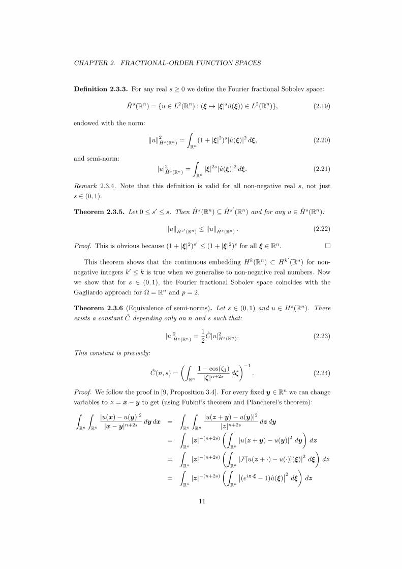
Definition 2.3.3. For any real s ≥ 0 we define the Fourier fractional Sobolev space:

Hs(Rn) = u ∈ L2(Rn) : (ξ 7→ |ξ|su(ξ)) ∈ L2(Rn), (2.19)

endowed with the norm:

‖u‖2Hs(Rn) =

∫Rn

(1 + |ξ|2)s|u(ξ)|2 dξ, (2.20)

and semi-norm:

|u|2Hs(Rn)

=

∫Rn|ξ|2s|u(ξ)|2 dξ. (2.21)

Remark 2.3.4. Note that this definition is valid for all non-negative real s, not just

s ∈ (0, 1).

Theorem 2.3.5. Let 0 ≤ s′ ≤ s. Then Hs(Rn) ⊆ Hs′(Rn) and for any u ∈ Hs(Rn):

‖u‖Hs′ (Rn) ≤ ‖u‖Hs(Rn) . (2.22)

Proof. This is obvious because (1 + |ξ|2)s′ ≤ (1 + |ξ|2)s for all ξ ∈ Rn.

This theorem shows that the continuous embedding Hk(Rn) ⊂ Hk′(Rn) for non-

negative integers k′ ≤ k is true when we generalise to non-negative real numbers. Now

we show that for s ∈ (0, 1), the Fourier fractional Sobolev space coincides with the

Gagliardo approach for Ω = Rn and p = 2.

Theorem 2.3.6 (Equivalence of semi-norms). Let s ∈ (0, 1) and u ∈ Hs(Rn). There

exists a constant C depending only on n and s such that:

|u|2Hs(Rn)

=1

2C|u|2Hs(Rn). (2.23)

This constant is precisely:

C(n, s) =

(∫Rn

1− cos(ζ1)

|ζ|n+2sdζ

)−1

. (2.24)

Proof. We follow the proof in [9, Proposition 3.4]. For every fixed y ∈ Rn we can change

variables to z = x− y to get (using Fubini’s theorem and Plancherel’s theorem):∫Rn

∫Rn

|u(x)− u(y)|2

|x− y|n+2sdy dx =

∫Rn

∫Rn

|u(z + y)− u(y)|2

|z|n+2sdz dy

=

∫Rn|z|−(n+2s)

(∫Rn|u(z + y)− u(y)|2 dy

)dz

=

∫Rn|z|−(n+2s)

(∫Rn|F [u(z + ·)− u(·)](ξ)|2 dξ

)dz

=

∫Rn|z|−(n+2s)

(∫Rn

∣∣(eiz·ξ − 1)u(ξ)∣∣2 dξ) dz

11

2.3. FOURIER TRANSFORM APPROACH

=

∫Rn

(∫Rn

|eiz·ξ − 1|2

|z|n+2sdz

)|u(ξ)|2 dξ

=

∫Rn

(∫Rn

(eiz·ξ − 1)(e−iz·ξ − 1)

|z|n+2sdz

)|u(ξ)|2 dξ

= 2

∫Rn

(∫Rn

1− cos(z · ξ)

|z|n+2sdz

)|u(ξ)|2 dξ. (2.25)

Now consider the rotation matrixR for whichR(|ξ|e1) = ξ and perform the substitution

ζ = |ξ|RTz. Then

z · ξ = |ξ|−1Rζ ·R(|ξ|e1) = RTRζ · e1 = ζ1.

Hence, ∫Rn

1− cos(z · ξ)

|z|n+2sdz =

∫Rn

1− cos(ζ1)

|ζ/|ξ||n+2s

1

|ξ|ndζ

= |ξ|2s∫Rn

1− cos(ζ1)

|ζ|n+2sdζ

= |ξ|2sC(n, s)−1. (2.26)

Combining (2.25) and (2.26) gives:

|u|2Hs(Rn) = 2C(n, s)−1|u|2Hs(Rn)

, (2.27)

which completes the proof.

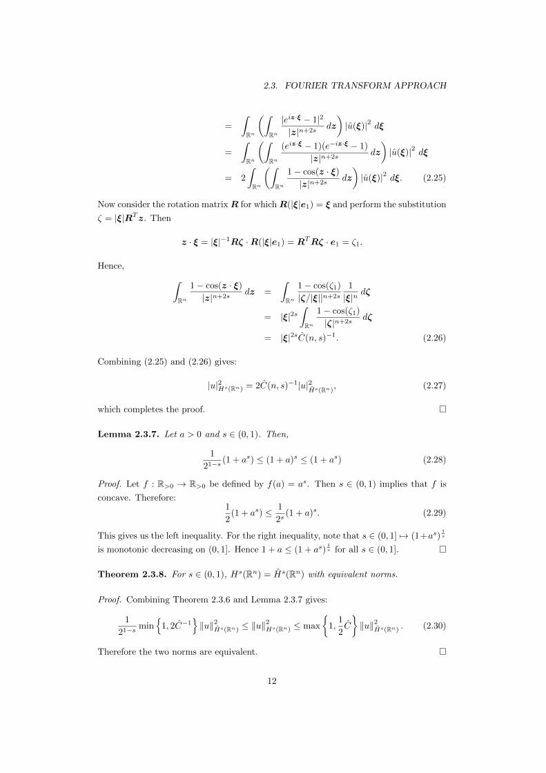
Lemma 2.3.7. Let a > 0 and s ∈ (0, 1). Then,

1

21−s (1 + as) ≤ (1 + a)s ≤ (1 + as) (2.28)

Proof. Let f : R>0 → R>0 be defined by f(a) = as. Then s ∈ (0, 1) implies that f is

concave. Therefore:1

2(1 + as) ≤ 1

2s(1 + a)s. (2.29)

This gives us the left inequality. For the right inequality, note that s ∈ (0, 1] 7→ (1+as)1s

is monotonic decreasing on (0, 1]. Hence 1 + a ≤ (1 + as)1s for all s ∈ (0, 1].

Theorem 2.3.8. For s ∈ (0, 1), Hs(Rn) = Hs(Rn) with equivalent norms.

Proof. Combining Theorem 2.3.6 and Lemma 2.3.7 gives:

1

21−s min

1, 2C−1‖u‖2Hs(Rn) ≤ ‖u‖

2Hs(Rn) ≤ max

1,

1

2C

‖u‖2Hs(Rn) . (2.30)

Therefore the two norms are equivalent.

12

CHAPTER 2. FRACTIONAL-ORDER FUNCTION SPACES

Corollary 2.3.9. Let 0 < s′ ≤ s < 1. Then Hs(Rn) ⊆ Hs′(Rn) and for u ∈ Hs(Rn):

‖u‖2Hs′ (Rn)

≤ ‖u‖2Hs(Rn) , (2.31)

where Cemb(s′, s) = 21−s max

1, 12 C(n, s′)

max

1, 1

2 C(n, s)

.

Remark 2.3.10. Continuous embeddings of this form can be proved for general W s,p(Ω)

spaces, if Ω is a bounded Lipschitz domain in Rn[9, Props. 2.1, 2.2, 2.3]. However, the

constants in the more general inequalities are difficult to find explicitly, which we value

highly for the computation of error bounds for approximation schemes.

2.4 Further properties of fractional Sobolev spaces

Here we present more theorems that will be of use to us later.

Theorem 2.4.1. For any s ≥ 0, C∞0 (Rn) is dense in W s,p(Rn)

Proof. See Sobolev Spaces, by Adams [1, Thm. 7.38].

Theorem 2.4.2. Let b ∈ W 1,∞(Ω). Then b is Lipschitz continuous with Lipschitz

constant ‖∇b‖∞.

Proof. Evans remarks that for general open subsets Ω of Rn, b ∈ W 1,∞loc (Ω) if and

only if b is Lipschitz continuous [17, p. 295]. Since W 1,∞(Ω) ⊆ W 1,∞loc (Ω) we have the

theorem.

Lemma 2.4.3. Let u ∈ Hs(Rn) and b ∈ W 1,∞(Rn). Then there exists a constant Cb,s

depending on s, n and b such that:

‖bu‖Hs(Rn) ≤ Cb,s ‖u‖Hs(Rn) . (2.32)

Further, the constant can be explicitly stated:

Cb,s = ‖b‖∞ ·

(1 +

2πn2

Γ(n2 )

(4

s+

1

1− s

(‖∇b‖∞‖b‖∞

)2)) 1

2

. (2.33)

Proof. This proof takes ideas from [9, Lemma 5.3]. It is straightforward to prove

‖bu‖L2(Rn) ≤ ‖b‖∞ ‖u‖L2(Rn). Now for the semi-norm:

|u|2Hs(Rn) =

∫Rn

∫Rn

|b(x)u(x)− b(y)u(y)|2

|x− y|n+2sdy dx

≤ 2

∫Rn

∫Rn

|b(x)u(x)− b(x)u(y)|2

|x− y|n+2sdy dx

+2

∫Rn

∫Rn

|b(x)u(y)− b(y)u(y)|2

|x− y|n+2sdy dx

13

2.5. TRACES AND FRACTIONAL SOBOLEV SPACES

≤ 2

(‖b‖2∞|u|2Hs(Rn) +

∫Rn

∫Rn|u(x)|2 |b(x)− b(y)|2

|x− y|n+2sdy dx

).

We used the inequality (a+ b)2 < 2a2 +2b2 for the second line. Now we can do a change

of variables z = y − x, and use the Theorem 2.4.2 for |z| ≤ 1:∫Rn

∫Rn|u(x)|2 |b(x)− b(y)|2

|x− y|n+2sdy dx =

∫Rn|u(x)|2

∫Rn

|b(x)− b(z + x)|2

|z|n+2sdz dx

≤ ‖u‖2L2(Rn) ‖∇b‖2∞

∫|z|≤1

|z|−n+2(1−s) dz

+ ‖u‖2L2(Rn) 22‖b‖2∞∫|z|>1

|z|−n−2s dz

= ‖u‖2L2(Rn) ‖∇b‖2∞

2πn2

Γ(n2 )

∫ 1

0

r2(1−s)−1 dr

+4 ‖u‖2L2(Rn) ‖b‖2∞

2πn2

Γ(n2 )

∫ ∞1

r−2s−1 dr

= ‖u‖2L2(Rn) ‖∇b‖2∞

πn2

Γ(n2 )

1

1− s

+ ‖u‖2L2(Rn) ‖b‖2∞

πn2

Γ(n2 )

4

s.

We used the formula for the surface area of the unit hypersphere in Rn for a change of

variables to hyperspherical coordinates. Collecting these inequalities:

‖bu‖2Hs(Rn) ≤ ‖u‖2L2(Rn)

(‖b‖2∞ + 2‖∇b‖2∞

πn2

Γ(n2 )

1

1− s+ 2‖b‖2∞

πn2

Γ(n2 )

4

s

)+2‖b‖2∞|u|2Hs(Rn)

≤ C2b,s ‖u‖

2Hs(Rn) .

For the final step we have used the fact that:

2πn2

Γ(n2 )

4

s≥ 1.

This completes the proof.

2.5 Traces and fractional Sobolev spaces

A linear operator T , which maps a function u defined on Ω to u∂Ω, its restriction to the

boundary, is called a trace operator. For continuous functions this is a trivial operation

as there is a natural embedding C(Ω) → C(∂Ω).

Now, for a function in W 1,p(Ω), the interpretation of a trace operator isn’t so sim-

ple. Sobolev spaces are a subspace of Lebesgue spaces, so firstly its elements are not

necessarily continuous and secondly they are not necessarily defined everywhere on Ω.

14

CHAPTER 2. FRACTIONAL-ORDER FUNCTION SPACES

Consider the operator T : C1(Ω) → Lp(∂Ω) defined as above. Recall from the C5.1a

course [34], that if this operator is continuous, then we can extend T uniquely to the clo-

sure of C1(Ω) in W 1,p(Ω), namely the space itself, W 1,p(Ω), giving us the a continuous

trace operator T : W 1,p(Ω)→ Lp(∂Ω). We need the following definition.

Definition 2.5.1 ([9]). Let Ω be an open subset of Rn. We say that Ω is of class Ck,σ

for k ∈ N, σ ∈ [0, 1] if the exists a positive constant M such that for every x ∈ ∂Ω, there

exists r > 0 and an isomorphism S : C → B(x; r) such that:

S ∈ Ck,σ(C), S−1 ∈ Ck,σ(B(x; r)),

B(x; r) ∩ Ω = S(C+), B(x; r) ∩ ∂Ω = S(C0),

‖S‖Ck,σ(C) + ‖S−1‖Ck,σ(B(x;r))

≤M,

where C is the cylinder:

C :=x = (x, xn) ∈ Rn−1 × R : |x| < 1 and |xn| < 1

,

and

C+ := x ∈ C : xn > 0 , C0 := x ∈ C : xn = 0 .

Essentially, if Ω is a domain described above, we can transplant any theorem for

the boundary ∂Ω to a theorem for the flat boundary C0 of the domain C+, with the

smoothness and regularity assumptions for S controlling how “nice” the transformation

is.

We learned in the C5.1a course that if Ω is a C1,0 domain with bounded boundary,

then there is a continuous trace operator from W 1,p(Ω) to Lp(Ω). Domains with C1,0

boundary cannot have any sharp edges, which is restrictive because for approximation

schemes we often solve on a polygonal domain.

Thankfully, the result extends to bounded Lipschitz domains (i.e. C0,1 domains).

These domains are allowed to have sharp edges like a polygon, but not cusps. It also

extends to fractional values of s: The following theorem for the special case of p = 2 is

due to Gagliardo (1957) [18].

Theorem 2.5.2 (The trace theorem). Let 12 < s ≤ 1 and let Ω be a bounded Lipschitz

domain. Then there exists a continuous, surjective trace operator

T : Hs(Ω)→ Hs− 12 (∂Ω). (2.34)

Remark 2.5.3. The theorem is in fact true for 12 < s < 3

2 (see [10]).

For s ∈ (0, 12 ], we have no such theorem. There is no continuous trace operator on

Hs(Ω) into a Lebesgue space for any Ω ⊆ Rn. Therefore, boundary conditions such as

u = g on ∂Ω (2.35)

15

2.6. THE IMPORTANCE OF THE CASE S ∈ (0, 12 )

do not make sense for any measurable function g on ∂Ω. Therefore when s ∈ (0, 12 ],

we must extend our notion of a boundary condition for the case s < 12 . We introduce

volume-constrained problems in Chapter 5.

2.6 The importance of the case s ∈ (0, 12)

One reason one may wish to study FDEs with weak solutions in the space Hs(Ω) for

s ∈ (0, 12 ), despite the difficulties with boundary conditions is that they may have jump

discontinuities [11, Sec. 1.1]. Discontinuous solutions occur in many modelling problems

(e.g. shocks) and it may be that the discontinuities arise due to the regularity of the

modelled function being less than 12 . Consider the following simple example:

Proposition 2.6.1. χ[0,1] ∈ Hs(R) if and only if s ∈ (0, 12 ).

Proof. An exercise for the reader.

This gives us some intuitive reason as to why there are no continuous trace operators

on Hs(Ω) with s < 12 . Consider a hypothetical trace operator T from Hs(0, 1) to 0, 1,

let fn = χ[1/n,1] ∈ Hs(0, 1) for n = 1, 2 . . . and let f = χ[0,1] ∈ Hs(0, 1). Then, noting

that f = fn on [ 1n , 1] and fn = 0 on [0, 1

n ], we have:

‖f − fn‖2Hs(0,1) =

(1

n

)2

+ 2

∫ 1n

0

∫ 1

1n

1

(y − x)1+2sdy dx

=

(1

n

)2

+2

2s

∫ 1n

0

1

( 1n − x)2s

− 1

(1− x)2sdx

=

(1

n

)2

+2

2s(1− 2s)

((1

n

)1−2s

− 11−2s − 01−2s +

(1− 1

n

)1−2s)

→ 0 as n→ 0.

Therefore fn → f , but T (fn)(0)→ 0 6= 1 = T (f)(0). So T is not continuous.

16

Chapter 3

Fractional-Order Operators

The main aim of this chapter is to note some useful results for operators with fractional

order, and to prove the fractional Friedrichs inequality with an explicit constant.

3.1 The Riemann-Liouville fractional derivative

Here we briefly give motivation behind the notion of fractional integration and differenti-

ation due to Riemann and Liouville (independently [31, p. 116]). This section will leave

a lot to the reader, should they decide to prove all the propositions. We use phrases like

“it is an easy exercise” because we merely want to motivate the technical discussion in

the next section, and the proofs are straightforward anyway.

Let f ∈ C∞([a, b]) for some real numbers a < b and define the integration operator,

Ja : C∞([a, b])→ C∞([a, b]):

Jaf =

∫ x

a

f(t)dt. (3.1)

It is an easy exercise to show that Ja is a continuous linear operator with ‖Ja‖ = b−a. It

is also an easy exercise, using Fubini’s theorem, to prove Cauchy’s formula for repeated

integration:∫ x

a

∫ x1

a

. . .

∫ xk−1

a

f(xk) dxk . . . dx2 dx1 =1

(k − 1)!

∫ x

a

(x− t)k−1f(t) dt. (3.2)

In fact, the proof of (3.2) was a set problem in the B4a Banach Spaces course in 2010.

So we can define an operator J (−k)a : C∞([a, b])→ C∞([a, b]), for each integer k > 0, by

J (−k)a f =

1

(k − 1)!

∫ x

a

(x− t)k−1f(t) dt. (3.3)

We use −k to denote the differential order of J (−k)a = J ka .

17

3.1. THE RIEMANN-LIOUVILLE FRACTIONAL DERIVATIVE

Now we would like to generalise this to obtain a fractional integral operator. Recall

the definition of Euler’s Gamma function,

Γ(s) =

∫ ∞0

ts−1e−t dt, (3.4)

which extends the factorial function to all positive integers (and in fact, to the complex

plane minus the non-positive integers). We have that Γ(1) = 1 and sΓ(s) = Γ(1 + s) for

all s > 0, so for s ∈ N, Γ(s) = (s− 1)!1.

Now we can define, for s > 0,

J (−s)a f =

1

Γ(s)

∫ x

a

(x− t)s−1f(t) dt. (3.5)

This integral is finite because we are on a bounded domain, and the operator coincides

with that in (3.3) for integer values of s. We call (3.5) the Riemann-Liouville fractional

integral of order s.

What about fractional derivatives? We cannot simply use the same formula for

negative values of s; the integral is not finite. However, there is nice trick we can use.

If we want a fractional derivative of order s ∈ (0, 1), then we can define the operator as

the composition of a fractional integral of order 1− s and a first-order derivative:

J (s)a f =

1

Γ(1− s)d

dx

∫ x

a

(x− t)−sf(t) dt, (3.6)

and similarly for any non-integral s > 0, if k is the unique integer such that k−1 < s < k,

we can define:

J (s)a f =

1

Γ(k − s)dk

dxk

∫ x

a

(x− t)k−s−1f(t) dt. (3.7)

This is called the Riemann-Liouville fractional derivative of order s. For integral s we

must use the classical definition of a derivative. Notice the nonlocality we discussed in

the introduction: J (s)a f(x) depends on all the values of f in the range [a, x].

It turns out that we can simplify a lot of the theory that stems from such a definition

by setting a = −∞, but still only considering functions on a compact domain. If we

want to extract the integral or derivative with arbitrary a, we can use the fact that:

J (−s)a f(x) = J (−s)

−∞ f(x)− J (−s)−∞ f(a). This setting also allows us to make the following

link between the Gamma function and the fractional derivative. A change of variables

in (3.5) gives:

J (−s)−∞ f =

1

Γ(s)

∫ ∞0

ts−1f(x− t) dt. (3.8)

If we let f(x) = ex, then

J (−s)−∞ ex =

ex

Γ(s)

∫ ∞0

ts−1e−t dt = ex, (3.9)

1It therefore isn’t technically an extension of the factorial function. According to Wikipedia, this

quirk is due to Legendre, for reasons that are unclear.

18

CHAPTER 3. FRACTIONAL-ORDER OPERATORS

and the same holds for the fractional derivatives. So we can consider the division by

Γ(s) to be a normalisation of the fractional integral and derivative in order to make ex

invariant under such operations.

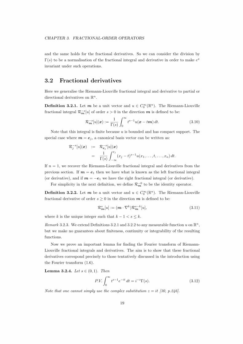
3.2 Fractional derivatives

Here we generalise the Riemann-Liouville fractional integral and derivative to partial or

directional derivatives on Rn.

Definition 3.2.1. Let m be a unit vector and u ∈ C∞0 (Rn). The Riemann-Liouville

fractional integral R−sm [u] of order s > 0 in the direction m is defined to be:

R−sm [u](x) :=1

Γ(s)

∫ ∞0

ts−1u(x− tm) dt. (3.10)

Note that this integral is finite because u is bounded and has compact support. The

special case where m = ej , a canonical basis vector can be written as:

R−sj [u](x) := R−sej [u](x)

=1

Γ(s)

∫ xj

−∞(xj − t)s−1u(x1, . . . , t, . . . , xn) dt.

If n = 1, we recover the Riemann-Liouville fractional integral and derivatives from the

previous section. If m = e1 then we have what is known as the left fractional integral

(or derivative), and if m = −e1 we have the right fractional integral (or derivative).

For simplicity in the next definition, we define R−0m to be the identity operator.

Definition 3.2.2. Let m be a unit vector and u ∈ C∞0 (Rn). The Riemann-Liouville

fractional derivative of order s ≥ 0 in the direction m is defined to be:

Rsm[u] := (m · ∇k)Rs−km [u], (3.11)

where k is the unique integer such that k − 1 < s ≤ k.

Remark 3.2.3. We extend Definitions 3.2.1 and 3.2.2 to any measurable function u on Rn,

but we make no guarantees about finiteness, continuity or integrability of the resulting

functions.

Now we prove an important lemma for finding the Fourier transform of Riemann-

Liouville fractional integrals and derivatives. The aim is to show that these fractional

derivatives correspond precisely to those tentatively discussed in the introduction using

the Fourier transform (1.6).

Lemma 3.2.4. Let s ∈ (0, 1). Then

P.V.

∫ ∞0

ts−1e−it dt = i−sΓ(s). (3.12)

Note that one cannot simply use the complex substitution z = it [30, p.246].

19

3.2. FRACTIONAL DERIVATIVES

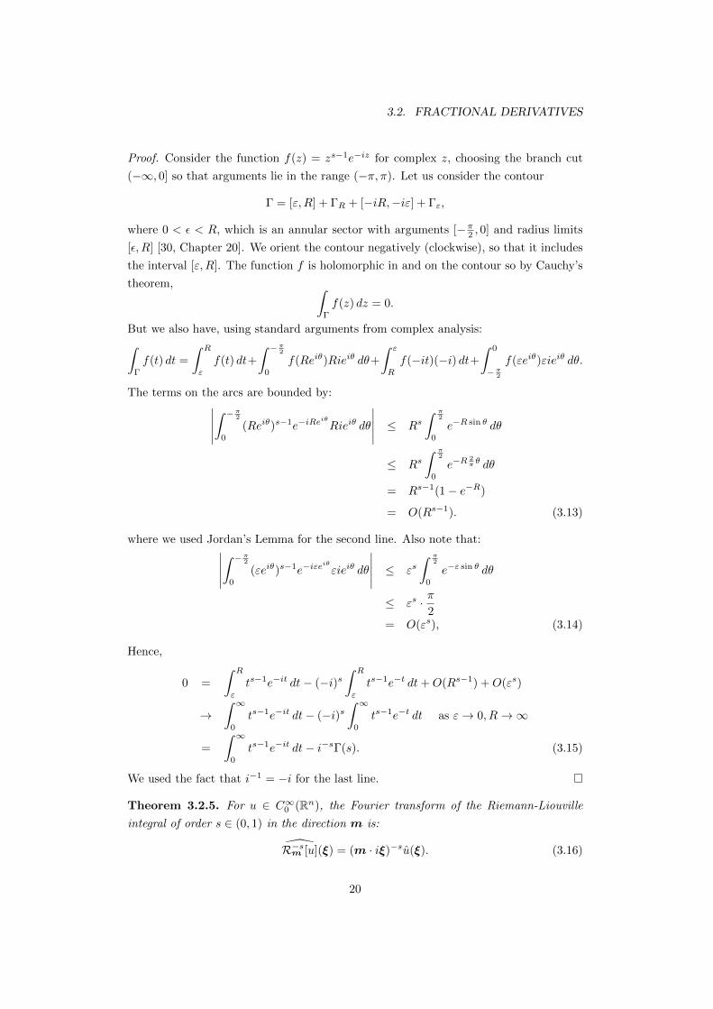
Proof. Consider the function f(z) = zs−1e−iz for complex z, choosing the branch cut

(−∞, 0] so that arguments lie in the range (−π, π). Let us consider the contour

Γ = [ε,R] + ΓR + [−iR,−iε] + Γε,

where 0 < ε < R, which is an annular sector with arguments [−π2 , 0] and radius limits

[ε, R] [30, Chapter 20]. We orient the contour negatively (clockwise), so that it includes

the interval [ε,R]. The function f is holomorphic in and on the contour so by Cauchy’s

theorem, ∫Γ

f(z) dz = 0.

But we also have, using standard arguments from complex analysis:∫Γ

f(t) dt =

∫ R

ε

f(t) dt+

∫ −π20

f(Reiθ)Rieiθ dθ+

∫ ε

R

f(−it)(−i) dt+∫ 0

−π2f(εeiθ)εieiθ dθ.

The terms on the arcs are bounded by:∣∣∣∣∣∫ −π2

0

(Reiθ)s−1e−iReiθ

Rieiθ dθ

∣∣∣∣∣ ≤ Rs∫ π

2

0

e−R sin θ dθ

≤ Rs∫ π

2

0

e−R2π θ dθ

= Rs−1(1− e−R)

= O(Rs−1). (3.13)

where we used Jordan’s Lemma for the second line. Also note that:∣∣∣∣∣∫ −π2

0

(εeiθ)s−1e−iεeiθ

εieiθ dθ

∣∣∣∣∣ ≤ εs∫ π

2

0

e−ε sin θ dθ

≤ εs · π2

= O(εs), (3.14)

Hence,

0 =

∫ R

ε

ts−1e−it dt− (−i)s∫ R

ε

ts−1e−t dt+O(Rs−1) +O(εs)

→∫ ∞

0

ts−1e−it dt− (−i)s∫ ∞

0

ts−1e−t dt as ε→ 0, R→∞

=

∫ ∞0

ts−1e−it dt− i−sΓ(s). (3.15)

We used the fact that i−1 = −i for the last line.

Theorem 3.2.5. For u ∈ C∞0 (Rn), the Fourier transform of the Riemann-Liouville

integral of order s ∈ (0, 1) in the direction m is:

R−sm [u](ξ) = (m · iξ)−su(ξ). (3.16)

20

CHAPTER 3. FRACTIONAL-ORDER OPERATORS

Proof. We can directly calculate:

R−sm [u](ξ) =1

(2π)n/2

∫Rne−ix·ξ

1

Γ(s)limR→∞

∫ R

0

ts−1u(x− tm) dt dx

=1

Γ(s)

1

(2π)n/2limR→∞

∫Rn

∫ R

0

e−ix·ξts−1u(x− tm) dt dx,

by the Dominated Convergence Theorem because u has compact support. In fact, if u

has support in the ball B(0, T ) for some T > 0 then we have that u(x− tm) has support

in B(0, T +R) for all t ∈ [0, R], so we have∫Rn

∫ R

0

∣∣e−ix·ξts−1u(x− tm)∣∣ dt dx ≤ |B(0, T +R)| · ‖u‖∞ ·

Rs

s<∞.

We can therefore use Fubini’s theorem to change the order of integration:

R−sm [u](ξ) =1

Γ(s)limR→∞

∫ R

0

ts−1 1

(2π)n/2

∫Rne−ix·ξu(x− tm) dx dt

=1

Γ(s)limR→∞

∫ R

0

ts−1F [u(x− tm)] dt

=

(1

Γ(s)limR→∞

∫ R

0

ts−1e−i(m·ξ)t dt

)u(ξ)

=

(1

Γ(s)limR→∞

∫ R

0

ts−1e−it dt

)(m · ξ)−su(ξ)

=

(1

Γ(s)P.V.

∫ ∞0

ts−1e−it dt

)(m · ξ)−su(ξ)

= (m · iξ)−su(ξ), (3.17)

using Lemma 3.2.4 for the last line.

Theorem 3.2.6. For u ∈ C∞0 (Rn), the Fourier transform of the Riemann-Liouville

derivative of order s ≥ 0 in the direction m is

Rsm[u](ξ) = (m · iξ)su(ξ). (3.18)

Proof. Let k be the unique integer such that k − 1 < s ≤ k. Then

Rsm[u](ξ) = F [(m · ∇k)Rs−km [u]](ξ)

= (m · iξ)kRs−km [u](ξ)

= (m · iξ)k(m · iξ)s−ku(ξ)

= (m · iξ)su(ξ).

21

3.2. FRACTIONAL DERIVATIVES

Remark 3.2.7. The Fourier transform of the integrals of order s ≥ 1 are of the same

form. It follows easily from the semi-group property of the fractional integral operator:

R−smR−s′

m = R−s−s′m for all s, s′ > 0 (see [16, Thm. 2.1]), which we won’t prove here.

The identity holds when applied to any measurable function u.

Theorem 3.2.8. The Riemann-Liouville fractional derivative Rsm for s ≥ 0 can be

extended to a continuous linear map from Hs(Rn) to L2(Rn).

Proof. First consider u ∈ C∞0 (Rn). Then, by Theorem 3.2.6 we have:

‖Rsm[u]‖L2(Rn) = ‖|m · ξ|su‖L2(Rn)

≤ ‖|ξ|su‖L2(Rn)

= |u|Hs(Rn). (3.19)

By Theorem 2.3.8 we have that ‖Rsm[u]‖L2(Rn) ≤ C ‖u‖Hs(Rn) for some constant C. By

the density Theorem 2.4.1 we can extend Rsm to a continuous linear operator on the

whole space Hs(Rn) with the same norm and the same bound as in (3.19).

Corollary 3.2.9. For u ∈ Hs(Rn), s ≥ 0, the Fourier transform of the Riemann-

Liouville fractional derivative is the same as in Theorem 3.2.6.

Proof. Let u ∈ Hs(Rn). Then, there is a sequence φj ⊂ C∞0 (Rn) such that φj → u in

Hs(Rn). Then we have∥∥∥(m · iξ)su− Rsmu∥∥∥L2(Rn)

≤∥∥∥(m · iξ)s(u− φj)

∥∥∥L2(Rn)

+∥∥∥Rsmφj − Rsmu∥∥∥

L2(Rn)

≤ 2|u− φj |Hs(Rn)

→ 0 as j →∞. (3.20)

We used the bound from (3.19) to get the second line.

Theorem 3.2.10 (Inversion property). Let s ≥ 0 and u ∈ C∞0 (Rn). Then,

R−smRsmu = u. (3.21)

Proof. For u ∈ C∞0 (Rn), we can justifiably differentiate under the integral sign in the

definition of the fractional derivative to have:

R−smRsmu = R−sm (m · ∇k)Rs−km u

= R−smRs−km (m · ∇k)u.

Then, by the semi-group property mentioned in Remark 3.2.7, we have:

R−smRsmu = R−km (m · ∇k)u

= u,

with the last line being a classical fact.

22

CHAPTER 3. FRACTIONAL-ORDER OPERATORS

3.3 Fractional Friedrichs inequality

Recall from the C5.1a course [34, Lemma 6.14] the following Friedrichs inequality:

Theorem 3.3.1 (Friedrichs inequality). Let u ∈W k,p0 (Ω). Then

‖u‖Lp(Ω) ≤dk

k!|u|Wk,p(Ω), (3.22)

where d = diam(Ω).

We prove an analogue of this for fractional orders and p = 2. We denote (x, xn) :=

(x1, x2, . . . , xn) and begin with some lemmata.

Theorem 3.3.2. Let, f ∈ L1(a, b) and g ∈ Lp(a, b) where p ≥ 1 and −∞ ≤ a < b ≤ ∞.

Then f ∗ g ∈ Lp(a, b) and

‖f ∗ g‖p ≤ ‖f‖1‖g‖p. (3.23)

Proof. The inequality follows by a straightforward application of Fubini’s theorem and

Holder’s inequality.

Lemma 3.3.3. Let u ∈ L2(Rn) and x ∈ Rn be such that supp(u(x, ·)) ⊆ [0,∞). Then

for any d > 0 and any s ≥ 0,

‖R−sn [u](x, ·)‖L2(0,d) ≤ds

Γ(1 + s)‖u(x, ·)‖L2(0,d). (3.24)

Proof. The idea for this proof comes from [15, Lemma 2.6]. We use remark 3.2.3 since

u is not necessarily in C∞0 (Rn). Let us define, for t > 0:

Is(t) =ts−1

Γ(s). (3.25)

Then we have, using the fact that u(x, t) = 0 for t < 0:

R−sn [u](x) =1

Γ(s)

∫ xn

−∞(xn − t)s−1u(x, t) dt

=

∫ xn

0

1

Γ(s)(xn − t)s−1u(x, t) dt

= (Is ∗ u(x, ·))(xn), (3.26)

where the convolution is over the interval (0, d). Hence, using Theorem 3.3.2,

‖R−sn [u](x, ·)‖L2(0,d) = ‖Is ∗ u(x, ·)‖L2(0,d)

≤ ‖Is‖L1(0,d)‖u(x, ·)‖L2(0,d)

=ds

sΓ(s)‖u(x, ·)‖L2(0,d)

=ds

Γ(1 + s)‖u(x, ·)‖L2(0,d). (3.27)

23

3.3. FRACTIONAL FRIEDRICHS INEQUALITY

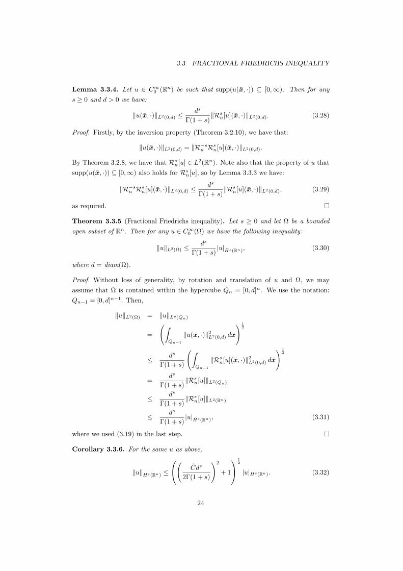
Lemma 3.3.4. Let u ∈ C∞0 (Rn) be such that supp(u(x, ·)) ⊆ [0,∞). Then for any

s ≥ 0 and d > 0 we have:

‖u(x, ·)‖L2(0,d) ≤ds

Γ(1 + s)‖Rsn[u](x, ·)‖L2(0,d). (3.28)

Proof. Firstly, by the inversion property (Theorem 3.2.10), we have that:

‖u(x, ·)‖L2(0,d) = ‖R−sn Rsn[u](x, ·)‖L2(0,d).

By Theorem 3.2.8, we have that Rsn[u] ∈ L2(Rn). Note also that the property of u that

supp(u(x, ·)) ⊆ [0,∞) also holds for Rsn[u], so by Lemma 3.3.3 we have:

‖R−sn Rsn[u](x, ·)‖L2(0,d) ≤ds

Γ(1 + s)‖Rsn[u](x, ·)‖L2(0,d), (3.29)

as required.

Theorem 3.3.5 (Fractional Friedrichs inequality). Let s ≥ 0 and let Ω be a bounded

open subset of Rn. Then for any u ∈ C∞0 (Ω) we have the following inequality:

‖u‖L2(Ω) ≤ds

Γ(1 + s)|u|Hs(Rn), (3.30)

where d = diam(Ω).

Proof. Without loss of generality, by rotation and translation of u and Ω, we may

assume that Ω is contained within the hypercube Qn = [0, d]n. We use the notation:

Qn−1 = [0, d]n−1. Then,

‖u‖L2(Ω) = ‖u‖Lp(Qn)

=

(∫Qn−1

‖u(x, ·)‖2L2(0,d) dx

) 12

≤ ds

Γ(1 + s)

(∫Qn−1

‖Rsn[u](x, ·)‖2L2(0,d) dx

) 12

=ds

Γ(1 + s)‖Rsn[u]‖L2(Qn)

≤ ds

Γ(1 + s)‖Rsn[u]‖L2(Rn)

≤ ds

Γ(1 + s)|u|Hs(Rn), (3.31)

where we used (3.19) in the last step.

Corollary 3.3.6. For the same u as above,

‖u‖Hs(Rn) ≤

( Cds

2Γ(1 + s)

)2

+ 1

12

|u|Hs(Rn). (3.32)

24

CHAPTER 3. FRACTIONAL-ORDER OPERATORS

Remark 3.3.7. This result also holds for the closure of C∞0 (Ω) with respect to the Hs(Rn)

norm. For integer-valued s = k ≥ 1 this space is Hk0 (Ω) and we recover the standard

Friedrichs inequality. we discuss this space for fractional values of s in Chapter 5.

Remark 3.3.8. Ervin and Roop prove the fractional Friedrichs inequality in one dimen-

sion in [15, Cor. 2.15] and two dimensions in [16, Cor. 5.3], but do not specify the

constant as we do.

3.4 The fractional Laplacian

Here we discuss the fractional Laplacian operator. For our definition of the fractional

Laplacian and derivation of the Fourier transform we follow [9, Sec. 3].

Definition 3.4.1. For u ∈ C∞0 (Rn) Laplacian of order s ∈ (0, 1) is:

(−∆)su := C(n, s) · P.V.∫Rn

u(x)− u(y)

|x− y|n+2sdy, (3.33)

where the principle value is taken as the limit of the integral over Rn \Bε(x) as ε→ 0.

Remark 3.4.2. The principle value is necessary in the definition if s ≥ 12 . For the integral

to be a Lebesgue integral for a given x, we require that in a neighbourhood Bε(x) of x

the following holds for some C, δ > 0:

|u(x)− u(y)| ≤ C|x− y|2s+δ, (3.34)

for then:

|u(x)− u(y)||x− y|n+2s

≤ C · χBε(x)(y) · |x− y|δ−n + χRn\Bε(x)(y) · 2‖u‖∞ · |x− y|−n−2s,

which is integrable over y ∈ Rn. Conversely, if (3.34) does not hold for any ε, then the

integrand is not integrable over any Bε(x). If s ∈ (0, 12 ) then (3.34) is satisfied by the

fact that u is Lipschitz. If s ≥ 12 , then as we noted in Remark 2.1.2, (3.34) implies that

u is constant in Bε(x). Having this for every x ∈ Rn implies u ≡ 0.

Now, by two changes of variables, z = y−x and z′ = x−y, we can rewrite (−∆)su

as:

(−∆)su =1

2C

(P.V.

∫Rn

u(x)− u(x+ z)

|z|n+2sdz + P.V.

∫Rn

u(x)− u(x− z′)|z′|n+2s

dz′)

=1

2C · P.V.

∫Rn

2u(x)− u(x+ y)− u(x− y)

|y|n+2sdy.

Using Taylor’s theorem to the second order, we have:

|2u(x)− u(x+ y)− u(x− y)| ≤ |y|2 · max|α|=2

maxy∈Rn

|Dαu(y)|. (3.35)

25

3.4. THE FRACTIONAL LAPLACIAN

Since u has compact support and |y|−n−2s+2 is integrable near 0 in Rn, we have the

Lebesgue integral:

(−∆)su =1

2C

∫Rn

2u(x)− u(x+ y)− u(x− y)

|y|n+2sdy. (3.36)

We proceed to compute the Fourier transform, but first we need a technical lemma:

Lemma 3.4.3. The integrand for the fractional Laplacian of u ∈ C∞0 (Rn) is integrable

over Rn × Rn:((x,y) 7→ 2u(x)− u(x+ y)− u(x− y)

|y|n+2s

)∈ L1(Rn × Rn). (3.37)

Proof. In the 19 November 2011 preprint of [9], the authors attempt a proof of this with

the following (quoted) argument:

|u(x+ y) + u(x− y)− 2u(x)||y|n+2s

≤ 4

(χB1

(y) · |y|2−n−2s · supB1(x)

|D2u|+ χRn\B1(y) · |y|−n−2s sup

Rn|u|

)≤ C

(χB1(y) · |y|2−n−2s

(1 + |x|n+1

)−1+ χRn\B1

(y) · |y|−n−2s)

∈ L1(Rn × Rn).

This argument is invalid, as the penultimate line is not integrable over the x variable.

They do not assume that u has compact support (they are working in what is known

as the Schwarz space on Rn, not C∞0 (Rn)). We do, so let u have support in the ball

B(0;T ) ⊂ Rn for some T > 0. Then∫Rn

|u(x+ y) + u(x− y)− 2u(x)||y|n+2s

dx

≤ |B(0;T + 1)| · χB1(y) · |y|2−n−2s · sup

B1(x)

|D2u|

+χRn\B1(y) · |y|−n−2s · 4 ·

∫Rn|u(x)| dx

≤ C(χB1

(y) · |y|2−n−2s + χRn\B1(y) · |y|−n−2s

)∈ L1(Rn). (3.38)

Then by Fubini’s Theorem [23, p. 25], we have the desired result.

Theorem 3.4.4. The Fourier transform of the fractional Laplacian of u ∈ C∞0 (Rn) is:

F [(−∆)su] (ξ) = |ξ|2su(ξ). (3.39)

Proof. We use a similar argument to the proof of Theorem 2.3.6, using the previous

lemma to switch the order of integration for the second line:

F [(−∆)su] =1

2C

∫Rn

∫Rne−ix·ξ

2u(x)− u(x+ y)− u(x− y)

|y|n+2sdy dx

26

CHAPTER 3. FRACTIONAL-ORDER OPERATORS

=1

2C

∫Rn|y|−n−2s

∫Rne−ix·ξ(2u(x)− u(x+ y)− u(x− y)) dx dy

=1

2C

∫Rn

F [2u(·)− u(·+ y)− u(· − y)]

|y|n+2sdy

=1

2C

∫Rn

(2− cos(y · ξ))u(ξ)

|y|n+2sdy.

We showed in Theorem 2.3.6 that:∫Rn

2− cos(y · ξ)

|y|n+2sdy = 2C−1|ξ|2s. (3.40)

This gives us the desired result.

Corollary 3.4.5. For s ∈ (0, 1), fractional Laplacian operator can be extended to a

continuous linear operator on H2s(Rn) with the same formula for the Fourier transform

as above.

Proof. The proof is based on using the technique in Theorem 3.2.8 and Corollary 3.2.9.

Remark 3.4.6. This theorem (and corollary) shows us that our “first attempt” at a

fractional Laplacian operator in the Introduction does indeed have an explicit form, and

it is a continuous operator on the fractional Sobolev space H2s(Rn).

Remark 3.4.7. The operator can be generalised to functions on any open subset Ω of

Rn, by taking the integral to be over Ω rather than Rn. However, the analysis of such

an operator is much harder because we cannot use the Fourier transform.

A finite element method for an isotropic anomalous advection-diffusion FDE, involv-

ing the fractional Laplacian operator (−∆)s, is discussed by Burrage et al. in [6].

Now, as we said in the introduction, we would like to have fractional-order oper-

ators that describe anisotropy, and also, operators with which we can create a weak

formulation of the advection-diffusion FDE. In the next chapter we describe a frame-

work developed by Du, Gunzburger, Lehouzq and Zhou (2011) [12] which enables us to

describe nonlocal, fractional-order operators of this sort.

27

Chapter 4

A Nonlocal Calculus

In this chapter we describe the nonlocal calculus of Du, Gunzburger, Lehoucq and Zhou

[12]. The point of the calculus is to define a general class of operators that behave like

the classical divergence, gradient and curl operators. To this end they satisfy nonlocal

analogues of the standard calculus theorems such as: integration by parts, Green’s

identities and Gauss’ divergence theorem.

In the classical calculus, these properties are essential for the weak formulation of

PDE problems. The main difference will be that the classical theorems involve functions

on the boundary of a domain, whereas these nonlocal versions involve functions on a

volume complementary to the domain which may or may not include the boundary.

Throughout this chapter we will consider the operators algebraically, and discuss

which spaces they act on and their analytical properties such as continuity later. For

the sake of argument one could assume all functions are infinitely differentiable with

compact support. We will let Ω be an open subset of Rn throughout, with its regularity

and smoothness discussed when necessary.

4.1 Notation

In the nonlocal calculus we consider two types of functions: those we call point functions,

that take one variable x from Rn, and those we call two-point functions, that take two

variables x and y from Rn. These functions can map to scalars, vectors or matrices,

and so things can become confusing as it is not always clear which domains functions

are mapping from or to. A carefully designed notational convention was used in [12],

which we follow also. For our purposes their guidelines can be reduced to the following

simplified system, which is also summarised in the table:

• Point vectors are denoted x,y, z ∈ Rn.

28

CHAPTER 4. A NONLOCAL CALCULUS

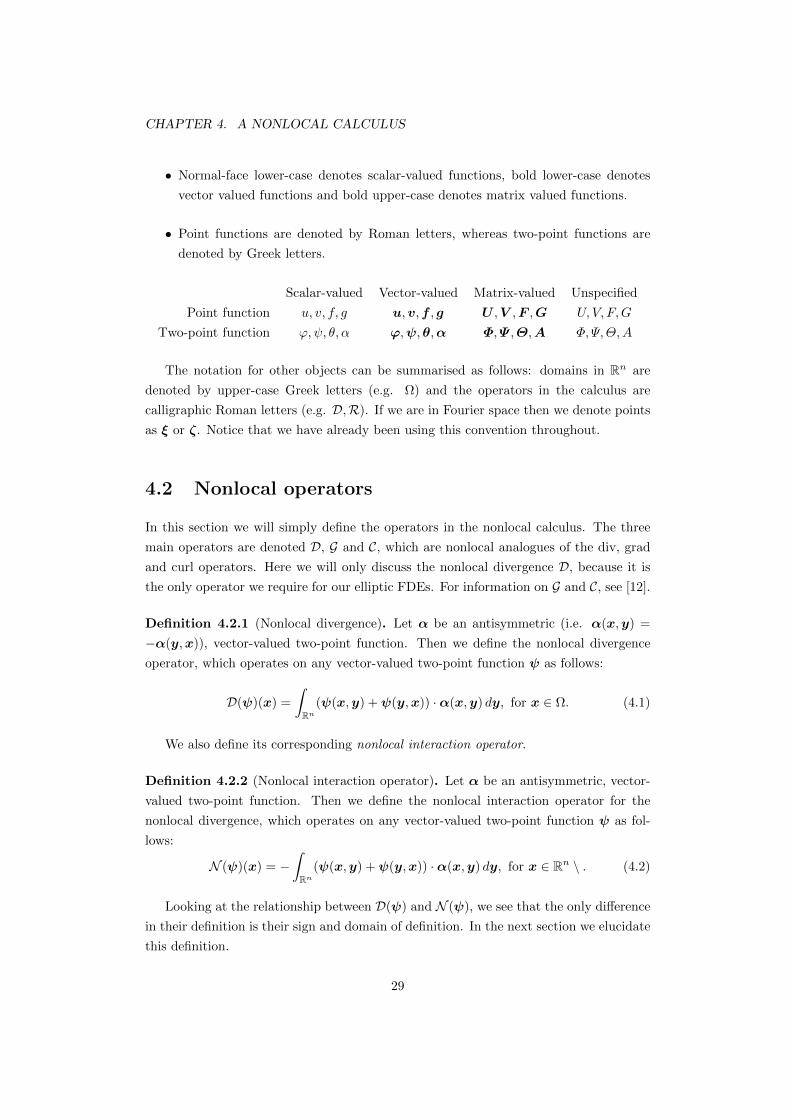
• Normal-face lower-case denotes scalar-valued functions, bold lower-case denotes

vector valued functions and bold upper-case denotes matrix valued functions.

• Point functions are denoted by Roman letters, whereas two-point functions are

denoted by Greek letters.

Scalar-valued Vector-valued Matrix-valued Unspecified

Point function u, v, f, g u,v,f , g U ,V ,F ,G U, V, F,G

Two-point function ϕ,ψ, θ, α ϕ,ψ,θ,α Φ,Ψ ,Θ,A Φ, Ψ,Θ,A

The notation for other objects can be summarised as follows: domains in Rn are

denoted by upper-case Greek letters (e.g. Ω) and the operators in the calculus are

calligraphic Roman letters (e.g. D,R). If we are in Fourier space then we denote points

as ξ or ζ. Notice that we have already been using this convention throughout.

4.2 Nonlocal operators

In this section we will simply define the operators in the nonlocal calculus. The three

main operators are denoted D, G and C, which are nonlocal analogues of the div, grad

and curl operators. Here we will only discuss the nonlocal divergence D, because it is

the only operator we require for our elliptic FDEs. For information on G and C, see [12].

Definition 4.2.1 (Nonlocal divergence). Let α be an antisymmetric (i.e. α(x,y) =

−α(y,x)), vector-valued two-point function. Then we define the nonlocal divergence

operator, which operates on any vector-valued two-point function ψ as follows:

D(ψ)(x) =

∫Rn

(ψ(x,y) +ψ(y,x)) ·α(x,y) dy, for x ∈ Ω. (4.1)

We also define its corresponding nonlocal interaction operator.

Definition 4.2.2 (Nonlocal interaction operator). Let α be an antisymmetric, vector-

valued two-point function. Then we define the nonlocal interaction operator for the

nonlocal divergence, which operates on any vector-valued two-point function ψ as fol-

lows:

N (ψ)(x) = −∫Rn

(ψ(x,y) +ψ(y,x)) ·α(x,y) dy, for x ∈ Rn \ . (4.2)

Looking at the relationship between D(ψ) and N (ψ), we see that the only difference

in their definition is their sign and domain of definition. In the next section we elucidate

this definition.

29

4.3. PROPERTIES OF THE NONLOCAL CALCULUS

4.3 Properties of the nonlocal calculus

The Gauss-Green Divergence Theorem for a vector-valued function f ∈ H1(Ω) is as

follows [17, p. 711]: ∫Ω

∇ · f dx =

∫∂Ω

m · f dS, (4.3)

where m is the outward unit normal vector for the C1 domain Ω. The following lemma

shows how the nonlocal operators are defined specifically to satisfy an analogous theorem.

Lemma 4.3.1 (Fundamental lemma of the nonlocal calculus). Any two-point function

Ψ ∈ L1(Rn × Rn), which is antisymmetric, has the following property:∫Rn

∫Rn

Ψ(x,y) dy dx = 0. (4.4)

Proof. First we use antisymmetry, then using Fubini’s theorem [23, p. 25] we can the

order of integration:∫Rn

∫Rn

Ψ(x,y) dy dx = −∫Rn

∫Rn

Ψ(y,x) dy dx

= −∫Rn

∫Rn

Ψ(y,x) dx dy

= −∫Rn

∫Rn

Ψ(x,y) dy dx. (4.5)

The last step is a relabelling of dummy variables.

Corollary 4.3.2 (Nonlocal divergence theorem). For D and N defined as in section

4.2 and any vector-valued two-point function ψ we have:∫Ω

D(ψ) dx =

∫Rn\Ω

N (ψ) dx. (4.6)

Proof. Note that α is antisymmetric and ψ(x,y) +ψ(y,x) is symmetric, so ψ(x,y) +

ψ(y,x)) ·α(x,y) is antisymmetric. Hence,∫Ω

D(ψ) dx−∫Rn\Ω

N (ψ) dx =

∫Rn

∫Rn

(ψ(x,y) +ψ(y,x)) ·α(x,y) dy dx = 0.

Rearranging gives us the desired equation.

For the classical calculus, we also have the integration by parts formula. For scalar-

valued u ∈ H1(Ω) and vector-valued v ∈ H1(Ω), this is the following:∫Ω

u(∇ · v) dx+

∫Ω

(−∇u) · v dx =

∫∂Ω

u(m · v) dS, (4.7)

where m is the outward unit normal vector for the C1 domain Ω. This equation can be

interpreted as saying that the negative gradient −∇ is a formal adjoint to the divergence

operator ∇·. Let us define the adjoint of a nonlocal operator in this way, and find it

explicitly, to have a nonlocal integration by parts formula.

30

CHAPTER 4. A NONLOCAL CALCULUS

Definition 4.3.3 (Nonlocal adjoint). For a nonlocal operator E with associated inter-

action operator X , its nonlocal adjoint is an operator E∗ such that, for functions Φ and

P : ∫Ω

PE(Φ) dx−∫Rn

∫RnE∗(P )Φdy dx =

∫Rn\Ω

PX (Φ) dx. (4.8)

Here Φ and P can be scalar- or vector-valued, depending on E .

Proposition 4.3.4 (Adjoint for nonlocal divergence). For D and N as defined in Sec-

tion 4.2, the adjoint for the nonlocal divergence is the operator D∗ such that for all

scalar-valued functions u:

D∗(u)(x,y) = (u(x)− u(y))α(x,y) ∀x,y ∈ Rn. (4.9)

Proof. Let ψ be a vector-valued two-point function. Then, using the fundamental

Lemma 4.3.1 to get the penultimate line,∫Ω

uD(ψ) dx−∫Rn\Ω

uN (ψ) dx

=

∫Rn

∫Rnu(x)(ψ(x,y) +ψ(y,x)) ·α(x,y) dy dx

=

∫Rn

∫Rn

(u(x)ψ(x,y)− u(y))ψ(x,y)) ·α(x,y) dy dx

+

∫Rn

∫Rn

(u(x)ψ(y,x) + u(y)ψ(x,y)) ·α(x,y) dy dx

=

∫Rn

∫Rn

(u(x)− u(y))α(x,y)ψ(x,y) dy dx

=

∫Rn

∫RnD∗(u)ψ(x,y) dy dx.

This completes the proof.

Corollary 4.3.5. [Nonlocal integration by parts] Let u be a scalar-valued one-point

function and let ψ be a vector-valued two-point function; then:∫Ω

uD(ψ) dx−∫Rn

∫RnD∗(u) ·ψ dy dx =

∫Rn\Ω

uN (ψ) dx. (4.10)

Proof. This is a restatement of Proposition 4.3.4.

From the integration by parts formula for classical derivatives, we can derive Green’s

first identity by setting v = A∇w for a matrix-valued function A ∈ C1(Ω) and a scalar-

valued function w ∈ H2(Ω):∫Ω

u(∇ ·A∇w) dx+

∫Ω

(−∇u) ·A∇w dx =

∫∂Ω

um ·A∇w dS, (4.11)

For the nonlocal calculus we can do the same by setting φ = ΘD∗(v) in the in-

tegration by parts formula, where v is a scalar-valued two-point function and Θ is a

matrix-valued two-point function (because D∗(v) is a two-point function).

31

4.4. INCLUSION OF THE CLASSICAL VECTOR CALCULUS

Theorem 4.3.6 (Nonlocal Green’s identity). Let D and N be the nonlocal divergence

and interaction operators as defined in Section 4.2, u and v scalar-valued one-point

functions and Θ a matrix-valued two-point functions. Then:∫Ω

uD(ΘD∗(v)) dx−∫Rn

∫RnD∗(u) ·ΘD∗(v) dy dx =

∫Rn\Ω

uN (ΘD∗(v)) dx (4.12)

Proof. Let ψ = ΘD∗(v) in Corollary 4.3.5.

Remark 4.3.7. Note that we use the entire complement of Ω (which is Rn \ Ω) for the

domain of the interaction function N (ψ). This means that in general there is no upper

limit on the distance of a nonlocal interaction. This need not be the case; for example if

α has support in the strip (x,y) : |x− y| < ε then nonlocal interactions are confined

within balls of radius ε. Then the interaction function N (ψ) has support in an ε-thin

strip surrounding Ω.

Given the theorems discussed in this section, we see a direct correspondence between

the operators of the nonlocal calculus: D, D∗ and N ; and those of the classical calcu-

lus: div, grad and the normal flux operator. In the next section we discuss how this

correspondence can be taken further.

4.4 Inclusion of the classical vector calculus

Du et al. showed that this nonlocal calculus generalises the classical vector calculus in

a distributional sense [12]. In other words, there is a choice of α (which is a distribu-

tion rather than a function) such that the nonlocal operators are effectively the classical

differential operators. By effectively we mean that this correspondence will not be per-

fect, because nonlocal operators involve two-point functions whereas classical differential

operators only involve one-point functions.

We try to be brief here to avoid losing focus; we include this discussion because we

take a slightly different approach to the one given in the original paper. Define the

antisymmetric α kernel to be the distribution:

α(x,y) = −∇yδ(y − x). (4.13)

This is “physicist’s notation” [34, p. 26] for the distribution Tα(x,·) such that for all

w ∈ C∞0 (Rn),

Tα(x,·)(w) = ∇ ·w(x) (4.14)

Again in physicist’s notation:

Tα(x,·)(w) =

∫Rnw(y) ·α(x,y) dy

=

∫Rnw(y) · (−∇y)δ(y − x) dy

32

CHAPTER 4. A NONLOCAL CALCULUS

=

∫Rn

(∇ ·w)δ(y − x) dy

= ∇ ·w(x).

We also define for each one-point function v a unique two-point function ϑv by the

formula:

ϑv(x,y) =1

2(v(x) + v(y)) . (4.15)

This next proposition shows that for any u,v ∈ C∞0 (Rn), we can desribe the diver-

gence, gradient and boundary conditions using the nonlocal opearators with the above

distributional definition for α.

Proposition 4.4.1. Let the divergence kernel α be defined by (4.13). Then for each

scalar-valued u ∈ C∞0 (Rn) and each vector-valued v ∈ C∞0 (Rn), the following hold in a

distributional sense:

∇ · v = D(ϑv), (4.16)

−∇u =

∫RnD∗(u) dy, (4.17)∫

∂Ω

u(m · v) dS =

∫Rn\Ω

uN (ϑv) dx, (4.18)

Proof. These identities can be proven in physicist’s notation by formal manipulations,

using the theorems discussed in the previous section in a distributional sense, along with

classical calculus theorems.

4.5 Anisotropic fractional Laplacian

In this section we describe the nonlocal operator we call the anisotropic fractional

Laplacian. Throughout, we let Θ be a matrix-valued symmetric two-point function

i.e. Θ(x,y) = Θ(y,x) for all x,y ∈ Rn.

Consider the following composition of nonlocal operators:

D(ΘD∗u)(x) =

∫Rn

2(u(x)− u(y))α(x,y) ·Θα(x,y) dy. (4.19)

The symmetry of Θ and the antisymmetry of α are essential for this identity. If we let

Θ be the identity matrix, and α be such that:

2|α(x,y)|2 =C(n, s)

|x− y|n+2s,

then the following holds:

D(D∗u)(x) = C(n, s)

∫Rn

u(x)− u(y)

|x− y|n+2sdy. (4.20)

33

4.5. ANISOTROPIC FRACTIONAL LAPLACIAN

We would like to deduce that the fractional Laplacian operator (−∆)s can be expressed

in the nonlocal calculus. However, we have a problem. The fractional Laplacian operator

is defined to be the principle value of this integral for u ∈ C∞0 (Rn) (see Definition 3.4.1)

and as we noted in Remark 3.4.2, the fractional Laplacian is only the proper Lebesgue

integral for each x ∈ Rn if s ∈ (0, 12 ), or u ≡ 0. This fact has been overlooked by Du et

al. in their discussion of the fractional Laplacian in the nonlocal calculus [11, A1], (or

perhaps they know of a trivial workaround).

In order to include the fractional Laplacian for s ≥ 12 in the nonlocal calculus, we

must make a modification: We change the integrals to principal value integrals. So let

us redefine the nonlocal divergence D to be as follows:

D(ψ)(x) = limε→0

∫Rn\Bε(x)

(ψ(x,y) +ψ(y,x)) ·α(x,y) dy, (4.21)

and the negative of this for N . This makes the nonlocal divergence and interaction

operators well-defined for the case ψ = D∗u, but not much more than this. All of the

theorems in Section 4.2 rely on the fundamental lemma, which itself relies on the use

of Fubini’s theorem, a theorem for Lebesgue integrable functions. In fact, consider the

two-point function ψ : R× R→ R defined by:

ψ(x, y) = χ[1,∞)×[1,∞)(x, y) · x2 − y2

(x2 + y2)2. (4.22)

This two-point function is antisymmetric, but is also a standard integration example

(see Part A Integration course) with:

0 6=∫R

∫Rψ(x, y) dy dx = −π

46= π

4=

∫R

∫Rψ(x, y) dx dy. (4.23)

Here the integrals are the principal value. We cannot even directly prove the Green’s

identity as a special case of the fundamental lemma; as we can see from the proof the

nonlocal adjoint (Proposition 4.3.4), we rely on the identity:∫Rn

∫Rn

(u(x)ψ(y,x) + u(y)ψ(x,y)) ·α(x,y) dy dx = 0 for all u, v, (4.24)

which, by setting ψ = D∗v for Green’s identity and α = αs, we have:∫Rn

∫Rn

(u(x) + u(y))(v(x)− v(y))

|x− y|n+2sdy dx = 0 for all u, v (4.25)

We cannot see any way to prove this, even if we assume u, v ∈ C∞0 (Ω). This technical

issue came to our attention very near to the submission date for this thesis, and we

have not been able to resolve it. Everything is well-defined and as it should be for

s ∈ (0, 12 ), but there certainly is a problem with using the nonlocal calculus for the

fractional Laplacian with s ∈ [ 12 , 1). Nonetheless we can still define the anisotropic

34

CHAPTER 4. A NONLOCAL CALCULUS

fractional Laplacian with the principal value version of the nonlocal divergence and

have a well-defined operator. Let us define the fractional kernel of order s ∈ (0, 1):

αs(x,y) =x− y

|x− y|n2 +s+1. (4.26)

Definition 4.5.1 (Anisotropic fractional Laplacian). Let Θ be a matrix-valued two-

point function, continuous and symmetric in its two arguments and satisfying the fol-

lowing ellipticity condition for some constants cΘ and CΘ:

∃cΘ, CΘ > 0 such that ∀x,y, z ∈ Rn, cΘ |z|2 ≤ zTΘ(x,y)z ≤ CΘ |z|2 . (4.27)

Let D be the nonlocal divergence operator with kernel αs, with principal values taken if

s ∈ [ 12 , 1). The anisotropic fractional Laplacian operator for Θ is the following operator:

u 7→ D(ΘD∗u). (4.28)

Remark 4.5.2. Note that the ellipticity condition on Θ implies that Θ(x,y) is a sym-

metric, positive definite matrix for every x and y. Therefore Θ defines a real inner

product matrix for each x and y. We can thence use the Cauchy-Schwarz inequality to

find:

zTΘz′ ≤ (zTΘz)12 (z′

TΘz′)

12 ≤ CΘ|z||z′| ∀z, z′ ∈ Rn. (4.29)

Explicitly, the definition of the anisotropic fractional Laplacian can be written:

D(ΘD∗u)(x) = P.V.

∫Rn

u(x)− u(y)

|x− y|n+2s· (x− y) ·Θ(x− y)

|x− y|2dy. (4.30)

As we can see, this operator generalises the fractional Laplacian by including a positive

weighting in the integral. It is difficult to find a space of functions within which 4.30 is

well defined and continuous, even for s ∈ (0, 12 ); for further work one could try to follow

a similar line of argument as in Theorem 3.4.4.

Since we cannot use the nonlocal Green’s identity for s ≥ 12 , we are going to have to

define the weak form of the anisotropic fractional Laplacian directly:

Definition 4.5.3. We define the anisotropic fractional Laplacian weakly on an open set

Ω for u ∈ Hs(Rn) by:∫Ω

vD(ΘD∗u) dx =

∫Rn

∫RnD∗v ·ΘD∗u dy dx for all v ∈ C∞0 (Ω). (4.31)

We can see that this weak operator is bounded on Hs(Rn) since:∫Rn

∫RnD∗v ·ΘD∗u dy dx ≤ CΘ ‖D∗v‖L2(Rn) ‖D

∗u‖L2(Rn) = CΘ|v|Hs(Rn)|u|Hs(Rn).

We can also see that for s ∈ (0, 12 ), the weak operator coincides with the anisotropic

fractional Laplacian in Definition 3.4.1 The nonlocal Green’s identity implies:∫Ω

vD(ΘD∗u) dx =

∫Rn

∫RnD∗v ·ΘD∗u dy dx+

∫Rn\Ω

vN (Θu) dx,

35

4.5. ANISOTROPIC FRACTIONAL LAPLACIAN

=

∫Rn

∫RnD∗v ·ΘD∗u dy dx. (4.32)

The following is a useful fact we use in Chapter 6:

Proposition 4.5.4. For the nonlocal divergence operator D with kernel αs, s ∈ (0, 1),

we have that D∗ is a continuous linear mapping from Hs(Rn) to L2(Rn × Rn).

Proof. Explicitly, for a scalar-valued one-point function u,

D∗u(x,y) = (u(x)− u(y))x− y

|x− y|n2 +s+1,

so: ∫Rn

∫Rn|D∗u(x,y)|2 dy dx =

∫Rn

∫Rn

|u(x)− u(y)|2

|x− y|n+2sdy dx = |u|2Hs(Rn). (4.33)

Therefore, for any u ∈ Hs(Rn), ‖D∗u‖L2(Rn×Rn) ≤ ‖u‖Hs(Rn).

36

Chapter 5

Volume-Constrained Problems

In this chapter we discuss the general form of some volume-constrained problems, and

reduce proving existence and uniqueness of solution to the non-homogeneous Dirichlet

volume-constrained problem to that of an homogeneous one.

5.1 Boundary value problems

This section will be slightly vague, as we use it just to motivate our treatment of the

volume-constrained problems. Dirichlet boundary-value problems on a bounded domain

Ω ⊂ Rn take the form of finding u in a function space V such that:

Lu = f in Ω,

u = g on ∂Ω.(5.1)

Here f and g are some prescribed functions defined on Ω and ∂Ω respectively, and Lis a differential operator. One way to start the analysis of such problems is to prove

that there exists a function g ∈ V defined on Ω such that g∂Ω = g. This follows from

surjectivity of a trace operator from V onto a space containing g (see Theorem 2.5.2).

Then we can rewrite the problem as follows:

Lu0 = f0 in Ω,

u0 = 0 on ∂Ω,(5.2)

where u0 = u− g and f0 = f −Lg [17, p. 315]. If we can prove existence and uniqueness

of a weak solution for this problem, then we have existence of a weak solution to problem

(5.1), which is u = u0 + g. By linearity of L, we also have uniqueness so long as 0 is

the unique solution to (5.1) with f ≡ 0 and g ≡ 0 (which follows from coercivity of the

bilinear form for the weak formulation).

37

5.2. VOLUME-CONSTRAINED PROBLEMS

For the particular case of V = H1(Ω), where Ω is a bounded Lipschitz domain, the

weak solutions to the homogeneous problem lie in the space:

H10 (Ω) :=

u ∈ H1(Ω) : Tu ≡ 0

. (5.3)

This is the space of zero-trace functions, where T is the trace operator on H1(Ω). One

can prove that for the case where Ω is a Lipschitz domain, this space is equal to the

closure of C∞0 (Ω) with respect to the H1(Ω) norm, which is denoted H10 (Ω) [17, p. 273].

Problems can then be tackled for C∞0 (Ω) functions before generalised to the whole of

the solution space by density.

We would like to do something similar for volume constrained problems: reduce the

problem to the homogeneous case and show that the homogeneous solution space has

dense subspace C∞0 (Ω).

5.2 Volume-constrained problems

Let Ω be a bounded open Lipschitz domain and let Ω be an open set containing the

closure of Ω. We denote Ωc = Ω\Ω ⊆ Rn\Ω. Let L be a differential operator of order 2s

where s ∈ (0, 1), f ∈ L2(Ω) and h ∈ Hs(Ωc). Consider the Dirichlet volume-constrained

problem:

Lu = f in Ω,

u = h in Ωc.(5.4)

As in the previous section, we would like to reduce this problem to the homogeneous

case where h ≡ 0. The volume Ωc shares some of it’s boundary with Ω by the way

we defined Ω, Ω and Ωc, which is Lipschitz by assumption. This is sufficient for the

existence of an extension of h into the whole of Ω by [9, Thm. 5.4]. Let this extension

be h ∈ Hs(Ω). Then we can restate the problem as:

Lu0 = f0 in Ω,

u0 = 0 in Ωc,(5.5)

where u0 = u − h and f0 = f − Lh. If we can prove existence and uniqueness of weak

solutions to this homogeneous Dirichlet problem (5.5) with u0 ∈ Hs(Ω) then we have

existence of the solution to the non-homogeneous problem (5.4) which we take to be

u = u0 + h. Further, if 0 is the unique solution to the homogeneous problem with f ≡ 0

then we have uniqueness of this solution u by linearity of L.

Weak solutions of the homogeneous problem (5.5) lie in the closed subspace:

HsΩ(Ω) :=

u ∈ Hs(Ω) : u = 0 on Ω \ Ω

. (5.6)

Now, before we go any further, we prove a result which reduces the problem further:

38

CHAPTER 5. VOLUME-CONSTRAINED PROBLEMS

Theorem 5.2.1. The space HsΩ(Ω) is isomorphic to Hs

Ω(Rn).

Proof. Define the linear operator T1 : HsΩ(Rn)→ Hs

Ω(Ω) by T1u = uΩ. This is a contin-

uous restriction mapping and therefore demonstrates that HsΩ(Rn) can be continuously

embedded into HsΩ(Ω).

Conversely consider the linear operator T2 : HsΩ(Ω)→ Hs

Ω(Rn) defined by:

T2u =

u in Ω,

0 in Rn \ Ω.(5.7)

Then we have ‖T2u‖L2(Rn) = ‖u‖L2(Ω) and using the fact that T2u = 0 in Rn \ Ω:

|T2u|2Hs(Rn) =

∫Ω

∫Ω

|u(x)− u(y)|2

|x− y|n+2sdy dx+ 2

∫Ω

∫Rn\Ω

|u(x)|2

|x− y|n+2sdy dx

≤ |u|2Hs(Ω)

+ 2

∫Ω

|u(x)|2∫Rn\Ω

1

dist(y,Ω)n+2sdy dx

≤ |u|2Hs(Ω)

+ 2‖u‖2L2(Ω)

∫Rn\Ω

1

dist(y,Ω)n+2sdy

≤ C(n, s, Ω) · ‖u‖2Hs(Ω)

. (5.8)

The last line is follows from the fact that Ω contains the closure of Ω, so since both

are open sets, dist(y,Ω) ≥ δ > 0 for all y ∈ Rn \ Ω. Hence, T2 is a continuous linear

operator demonstrating that HsΩ(Ω) can be continuously embedded into Hs

Ω(Rn).

By transitivity, all of the homogeneous Dirichlet volume-constrained spaces for Ω are

isomorphic. We see that for pure analysis these homogeneous problems, we can choose

whichever volume for Ω we want. In particular, we can choose the space HsΩ(Rn), which

has the useful Fourier transform characterisation.

Now, just as in the case of boundary value problems, we have that infinitely differ-

entiable functions with compact support in Ω is dense in our solution space:

Theorem 5.2.2. C∞0 (Ω) is dense in HsΩ(Rn) for s ∈ (0, 1).

Proof. This theorem can be found in Interpolation theory, function spaces and differen-

tial operators by Trievel, [37, p. 317,318]. Trievel uses Besov spaces, a generalisation of

fractional Sobolev spaces, so has different notation: HsΩ(Rn) is denoted by Bs2,2(Ω). By

Section 4.3.2, Theorem 1(b), C∞0 (Ω) is dense in Bs2,2(Ω), and so we have the result.

Remark 5.2.3. Trievel proves the theorem assuming the Ω is bounded with C∞ boundary.

This is so that he can consider all s in R (yes, including negative values!) without having

special cases for certain ranges of s. We have not checked fully, but we assume that a

bounded Lipschitz domain is sufficient for the theorem in the case s ∈ (0, 1).

In the next chapter we prove well-posedness of a general class of Dirichlet volume-

constrained elliptic problems of order 2s for s ∈ (0, 1).

39

Chapter 6

Well-Posedness of Elliptic

Problems

In this chapter we study a general class of elliptic FDEs of order 2s with s ∈ (0, 1). We

state the classical form for the homogeneous Dirichlet volume-constrained problem on

a bounded Lipschitz domain Ω ⊂ Rn, derive a weak formulation of the problem on the

space HsΩ(Rn) and prove existence and uniqueness of its solution. As explained in the

previous chapter, this implies existence and uniqueness for the nonhomogeneous case

too, if 0 is the unique solution to the completely homogeneous problem.

6.1 Classical statement of the Dirichlet problem

Let D(ΘD∗·) be an anisotropic fractional Laplacian operator defined as in Definition

4.5.3. Let f ∈ L2(Ω), b = (b1, . . . , bn)T ∈ C1(Ω), and c ∈ C(Ω). We consider two

separate cases:

• s ∈ [ 12 , 1), if b 6= 0

• s ∈ (0, 1), if b = 0

We wish to find a function u defined on Rn which satisfies the following problem at least

in a weak sense:

Lu := D(Θ(x,y)D∗u) + b(x) · ∇u+ c(x)u = f on Ω,

u = 0 on Rn \ Ω.(6.1)

The reason for the constraint on s is that the first-order advection term, which is present

if and only if b 6= 0, forces a weak solution u to require a regularity of at least 12 for our

well-posedness proof.

40

CHAPTER 6. WELL-POSEDNESS OF ELLIPTIC PROBLEMS

6.2 Weak formulation

In this section we define a bilinear operator on the Dirichlet volume-constrained Sobolev

space HsΩ(Rn) (Definition 5.6) which corresponds to (u, v) 7→

∫ΩvLu dx.

Let u be a weak solution to (6.1) and v ∈ C∞0 (Ω), then:∫Ω

vD(ΘD∗u) dx+

∫Ω

vb · ∇u dx +

∫Ω

cvu dx =

∫Ω

vf dx. (6.2)

By Definition 4.5.3, ∫Ω

vD(ΘD∗u) dx =

∫Rn

∫RnD∗v ·ΘD∗u dy dx. (6.3)

For the advection term, first note that v = 0 on Rn \ Ω, so:∫Ω

vb · ∇u dx =

∫Rnvb · ∇u dx

=n∑j=1

∫Rnvbj

∂u∂xj

dx. (6.4)

Now, using Parseval’s Theorem (A.3) along with the fact that vb is a real-valued function,

and then the Fourier transform of a partial derivative (Theorem A.4) we have:

n∑j=1

∫Rnvbj

∂u∂xj

dx =

n∑j=1

∫Rnvbj

∂u∂xj

dx

=

n∑j=1

∫Rnvbjiξj u dξ

=

n∑j=1

∫Rn

(−iξj)12 vbj(iξj)

12 u dξ. (6.5)

Here we used the following:

(iξj)12 = −i(iξj)

12 = (−i) 1

2 (−i2)12 (ξj)

12 = (−iξj)

12 . (6.6)

Using Corollary 3.2.9, we can express this in terms of Riemann-Liouville fractional

derivatives:n∑j=1

∫Rn

(−iξj)12 vbj(iξj)

12 u dξ =

n∑j=1

∫Rn

R

12−j(vbj)

R

12j (u) dξ

=

n∑j=1

∫RnR

12−j(vbj)R

12j (u) dx

=

n∑j=1

∫RnR

12−j(vbj)R

12j (u) dx. (6.7)

R12j is fractional derivative operator (3.2.2) of order 1

2 in the direction of the canonical

basis vector ej and that which we denote R12−j is that in the opposite direction, −ej .

Now we are ready to define a bilinear form to express the weak formulation of (6.1).

41

6.3. WELL-POSEDNESS OF THE WEAK FORMULATION

Definition 6.2.1. Let D(ΘD∗·) be an anisotropic fractional Laplacian operator defined

as in Definition 4.5.3. Let b ∈ W 1,∞(Ω) and c ∈ L∞(Ω). We define the bilinear form

for u, v ∈ HsΩ(Rn) by:

a(u, v) :=

∫Rn

∫RnD∗v ·ΘD∗u dy dx+

n∑j=1

∫RnR

12−j(vbj)R

12j (u) dx+

∫Ω

cvu dx, (6.8)

and for f ∈ L2(Ω), the linear functional l on HsΩ(Rn):

l(v) :=

∫Ω

vf dx. (6.9)

Definition 6.2.2 (Weak solution). Let a and l be as defined in (6.8) and (6.9). We call

u ∈ HsΩ(Rn) a weak solution to (6.1) if the following holds:

a(u, v) = l(v) ∀v ∈ HsΩ(Rn). (6.10)

6.3 Well-posedness of the weak formulation

Lemma 6.3.1. The bilinear form a is continuous.

Proof. By Theorem B.1 we only need to show that there exists a constant c1 such that

|a(u, v)| ≤ c1 ‖u‖Hs(Rn) ‖v‖Hs(Rn) for all u and v. Using the inequality derived in Remark

4.5.2 and the continuity of D∗ (Proposition 4.5.4), the diffusion term is controlled by

Sobolev semi-norms:∫Rn

∫Rn|D∗v ·ΘD∗u| dy dx ≤ CΘ

∫Rn

∫Rn|D∗v||D∗u| dy dx

≤ CΘ‖D∗v‖L2(Rn×Rn)‖D∗u‖L2(Rn×Rn)

= CΘ|v|Hs(Rn)|u|Hs(Rn). (6.11)

If b 6= 0, then by continuity of the Riemann-Liouville derivatives (Theorem 3.2.8) the

advection term is controlled by Sobolev norms:

n∑j=1

∫Rn|R

12−j(vbj)R

12j (u)| dx ≤

n∑j=1

(∫Rn|R

12−j(vbj)|

2 dx

) 12(∫

Rn|R

12−j(u)|2 dx

) 12

≤n∑j=1

|bjv|H

12 (Rn)

|u|H

12 (Rn)

=1

2C

(n,

1

2

) n∑j=1

|bjv|H

12 (Rn)

|u|H

12 (Rn)

≤ 1

2C

(n,

1

2

) n∑j=1

‖bjv‖H

12 (Rn)

‖u‖H

12 (Rn)

42

CHAPTER 6. WELL-POSEDNESS OF ELLIPTIC PROBLEMS

≤ 1

2C

(n,

1

2

) n∑j=1

Cbj , 12 ‖v‖H 12 (Rn)

‖u‖H

12 (Rn)

≤ C(b, n, s) ‖v‖Hs(Rn) ‖u‖Hs(Rn) , (6.12)

where

C(b, n, s) = Cemb

(s,

1

2

)C

(n,

1

2

) n∑j=1

Cbj , 12 . (6.13)

The constants and inequalities here come from Theorem 2.3.6, Theorem 2.4.3 and the

embedding Corollary 2.3.9. Finally, the reaction term is controlled by L2 norms:∫Ω

|cvu| dx ≤ ‖c‖∞∫

Ω

|vu| dx

≤ ‖c‖∞ ‖v‖L2(Ω) ‖u‖L2(Ω)

= ‖c‖∞ ‖v‖L2(Rn) ‖u‖L2(Rn) . (6.14)

Combining these bounds, we have:

a(u, v) ≤ CΘ|v|Hs(Rn)|u|Hs(Rn) + C(b, n, s) ‖v‖Hs(Rn) ‖u‖Hs(Rn) + ‖c‖∞ ‖v‖L2(Rn) ‖u‖L2(Rn)

≤((CΘ|v|Hs(Rn)

)2+(C(b, n, s) ‖v‖Hs(Rn)

)2

+(‖c‖∞ ‖v‖L2(Rn)

)2) 1

2

·(|u|2Hs(Rn) + ‖u‖2Hs(Rn) + ‖u‖2L2(Rn)

) 12

≤ c1 ‖v‖Hs(Rn) ‖u‖Hs(Rn) , (6.15)

where

c1 = 212 ·(max

C2Θ, ‖c‖2∞

+ C(b, n, s)2

) 12 . (6.16)

Note that we have derived an explicit form for this constant, which depends on Θ, b, c,

n, s, but not Ω.

Lemma 6.3.2. If c − 12∇ · b ≥ 0 then the bilinear functional a is coercive in Hs

Ω(Rn),

i.e. ∃c2 > 0 such that a(v, v) ≥ c2 ‖v‖2Hs(Rn) for all v ∈ HsΩ(Rn).

Proof. Assume for now that v ∈ C∞0 (Ω). We deal with the advection term with a

standard argument using integration by parts:

n∑j=1

∫RnR

12−j(vbj)R

12j (v) dx =

∫Ω

vb · ∇v dx

=

∫Ω

b · 1

2∇v2 dx

=

∫Ω

(−1

2∇ · b

)v2 dx. (6.17)

Then we directly show coercivity:

a(v, v) =

∫Rn

∫RnD∗v ·ΘD∗v dy dx+

n∑j=1

∫RnR

12−j(vbj)R

12j (v) dx+

∫Ω

cv2 dx.

43

6.3. WELL-POSEDNESS OF THE WEAK FORMULATION

=

∫Rn

∫RnD∗v ·ΘD∗v dy dx+

∫Ω

(c− 1

2∇ · b

)v2 dx

≥ cΘ

∫Rn

∫Rn|D∗v|2 dy dx

= cΘ|v|2Hs(Rn)

≥ c2 ‖v‖2Hs(Rn) . (6.18)

The last step is by the corollary of the fractional Friedrichs inequality for C∞0 (Ω) ⊂Hs

Ω(Rn) (Corollary 3.3.6). Note that we have derived an explicit form for the constant

c2, which depends on Θ, b, c, s and d, the diameter of Ω, but not n.

Now consider v ∈ HsΩ(Rn). C∞0 (Ω) is dense in Hs

Ω(Rn) (Theorem 5.2.2), so we have

a sequence vm∞m=0 ⊂ C∞0 (Ω) such that vm → v in Hs(Rn). By Lemma 6.3.1, a is

continuous, so:

a(v, v) = a( limm→∞

(vm, vm))

= limm→∞

a(vm, vm)

≥ c2 limm→∞

‖vm‖2Hs(Rn)

= c2 ‖v‖2Hs(Rn) . (6.19)

Therefore we have coercivity.

Lemma 6.3.3. The linear functional l is continuous.

Proof. Let v ∈ HsΩ(Rn). Then:

|l(v)| = |∫Ω

vf dx|

≤∫Ω

|vf | dx

≤ ‖f‖L2(Ω)‖v‖L2(Ω)

≤ ‖f‖L2(Ω)‖v‖Hs(Rn). (6.20)

Theorem 6.3.4 (Existence and uniqueness). If c− 12∇·b ≥ 0, then there exists a unique

weak solution to the homogeneous Dirichlet volume-constrained problem (6.1).

Proof. Collecting Lemmata 6.3.1, 6.3.2 and 6.3.3 gives us satisfaction of the conditions

for the Lax-Milgram Theorem (B.2). Therefore problem (6.10) has a unique solution.

Theorem 6.3.5 (Well-posedness). The weak formulation (6.10) is well-posed problem

in the sense of Hadamard [19], i.e. there exists a unique solution u in HsΩ(Rn) that

depends continuously on the data, f .

44

CHAPTER 6. WELL-POSEDNESS OF ELLIPTIC PROBLEMS

Proof. We showed in Theorem 6.3.4 above that there exists a unique solution to this

problem. For continuity, let uj be the solution to (6.10) with data fj for j = 1, 2. Then

by linearity u1 − u2 is the solution to (6.10) with l(v) =∫Ωv(f1 − f2) dx and so:

‖u1 − u2‖Hs(Rn) ≤|a(u1 − u2, u1 − u2)|c2‖u1 − u2‖Hs(Rn)

=|l(u1 − u2)|

c2‖u1 − u2‖Hs(Rn)≤ c−1

2 ‖f1 − f2‖L2(Ω).

(6.21)

Remark 6.3.6. Ervin and Roop [16, Sec. 6] study elliptic FDEs in two dimensions and

have a similar proof for existence and uniqueness of solution. The differences are: the

problems they study are boundary value problems, they only consider the case s ∈ ( 12 , 1)

and they use a different operator for the order 2s term, which is anisotropic, but the

anistropy does not depend on the location in the domain.

45

Chapter 7

Galerkin Approximation

7.1 Approximation of the problem

We wish to approximate the the weak formulation of the problem (6.10) by restricting

our consideration for our solution u and test functions v to a k-dimensional subspace Vk

of HsΩ(Rn) (for s ∈ (0, 1)), calling the approximate solution uk. We would then like to

prove that as k tends to infinity, these approximate solutions converge to the solution of

the actual problem in some suitable norm. This is a general approach called Galerkin’s

method [8, p. 36].

For now, we will assume nothing about Vk except its dimension and that it is a

subspace of HsΩ(Rn). Firstly, recall the weak formulation of our problem: Find u ∈

HsΩ(Rn) such that

a(u, v) = l(v) for all v ∈ HsΩ(Rn). (7.1)

Definition 7.1.1. We say that uk ∈ Vk is the Galerkin approximation to the solution

to (7.1) if:

a(uk, vk) = l(vk) for all vk ∈ Vk. (7.2)

Theorem 7.1.2. There exists a unique Galerkin approximation to u for each k.

Proof. We can use the Lax-Milgram Theorem (B.2), because the fact that a and l satisfy

the conditions for the theorem on HsΩ(Rn) imply they satisfy them on the subspace

Vk.

Remark 7.1.3. Recall from the C12.2b course that since Vk is finite dimensional, it has

a basis, and therefore the Galerkin approximation uk can be found by solving a system

of linear equations.

46

CHAPTER 7. GALERKIN APPROXIMATION

Definition 7.1.4. We say that the Galerkin approximation uk converges to the solution

u of (7.1) in the norm ‖ · ‖ on HsΩ(Rn) if:

‖u− uk‖HsΩ(Rn) → 0 as k →∞. (7.3)

7.2 Convergence in the Hs norm

The following lemma will give us a sufficient condition for convergence of the finite

element approximation in the Hs(Rn) norm.

Lemma 7.2.1 (Cea’s lemma). Let uk be the finite element approximation of (7.1),

and let c1 and c2 be the constants found in Lemmas 6.3.1 and 6.3.2 respectively for the

bilinear form a. Then:

‖u− uk‖Hs(Rn) ≤c1c2

infvk∈Vk

‖u− vk‖Hs(Rn) . (7.4)

Suppose futher that a is symmetric (i.e. b = 0). Then:

‖u− uk‖Hs(Rn) ≤√c1c2

infvk∈Vk

‖u− vk‖Hs(Rn) . (7.5)

Proof. See Finite Element Methods for Elliptic Problems, by Ciarley [8, Thm. 2.4.1,

Rmk. 2.4.1].

Theorem 7.2.2. A sufficient condition for convergence of the finite element approxi-

mation uk to the solution of (7.1) in the Hs(Rn) norm is that there exists a sequence of

operators Pk : HsΩ(Rn)→ Vk such that:

‖v − Pk(v)‖Hs(Rn) → 0 as k →∞, for all v ∈ HsΩ(Rn). (7.6)

Now we discuss examples of subspaces Vk and operators Pk such that this sufficient

condition holds.

7.3 Finite elements

As seen in the C12.2b course, we can consider the finite element spaces. We assume that

Ω is a polygonal domain, and triangulate it as usual with h > 0 being the length of the

longest side of any triangle in the mesh. The finite element space Vh ⊂ HsΩ(Rn) is the

space of all continuous, piecewise polynomials of degree m on the triangulation, where

m is a positive integer.

Theorem 7.3.1. Let s ∈ (0, 1), u ∈ HsΩ(Rn)). Then for real σ such that 0 ≤ s ≤ σ ≤ m

there exists a constant CI depending only on Ω such that:

‖u− Ihu‖Hs(Rn) ≤ CIhρ−s‖u‖Hσ(Ω) (7.7)

47

7.4. LEGENDRE POLYNOMIALS

Proof. See [4, Sec. 14.3] for a proof of:

‖u− Ihu‖Hs(Ω) ≤ Chρ−s‖u‖Hσ(Ω), (7.8)

for some constant C > 0. Then consider the theorem in [24, Thm. 11.4]. This theorem

implies that there exists a constant CΩ such that for any u ∈ HsΩ(Rn)

‖u‖Hs(Rn) ≤ CΩ‖u‖Hs(Ω). (7.9)

This gives the desired result with CI = C · CΩ.

The authors of [16] seem to have overlooked this issue. They quote the result (7.8),

but then use it as if the Hs(Ω) norm is equivalent to their Hs0(Ω) norm without justifi-

cation, which they define with the Fourier transform on R2.

7.4 Legendre polynomials

Let us consider the special case where Ω = [−1, 1], b = 0 and s ∈ (0, 12 ). The case s < 1

2

is interesting because the galerkin approximation need not be zero on the boundary (see

Section 2.6). It also simplifies matters because we don’t have to force our approximations

to have roots at −1 and 1. We can define the space Pk of polynomials of degree at most

k ∈ N and the operator Pk is the polynomial interpolant in k+ 1 Legendre points in Ω.

Theorem 7.4.1. Let s ∈ (0, 1), u ∈ HsΩ(Rn). Then for any real σ such that 0 ≤ s ≤ σ,

there exists a constant CP such that

‖u− Pku‖Hs(R) ≤ CPk3s/2−σ‖u‖Hσ(Ω). (7.10)

Proof. See [7, Thm. 2.4] for the bound:

‖u− Pku‖Hs(Ω) ≤ Ck3s/2−σ‖u‖Hσ(Ω), (7.11)

for some C > 0. Then note, as in Theorem 7.3.1, the continuous embedding of Hs(Ω)

into HsΩ(Rn) from [24, Thm. 11.4]. This gives the required inequality.

Corollary 7.4.2. Suppose that u is the solution to (7.1) for Ω = [−1, 1], b = 0 and

s ∈ (0, 12 ). Suppose further that u ∈ Hσ(Ω) where σ > 3s/2. Then the Galerkin

approximation uk to the problem (7.1) in the space Pk converges, and satisfies:

‖u− uk‖Hs(Rn) ≤√c1c2CPk

3s/2−σ‖u‖Hσ(Ω) (7.12)

Proof. Combine Cea’s Lemma 7.2.1 with the interpolation error estimate in Theorem

7.4.1.

48

Chapter 8

Conclusion

8.1 Aims of the project

When we proposed this project, we had an aim to develop a-posteriori error estimates

for a finite element method for an anomalous diffusion-type equation using the nonlocal

calculus. With these computable error estimates we wanted to implement an efficient

adaptive mesh algorithm.

However, the analysis of FDEs turned out to be much tougher than expected, pri-

marily because of the nonlocality of the fractional-order norms and operators, but it

certainly is interesting and it gave us a lot to study and write about. As a result, the

majority of this dissertation is devoted to the analytical side of FDEs, with just one

chapter devoted to approximation considerations.

8.2 Further work

We present ideas for further work in the form of a list:

• The issue with the nonlocal calculus for expressing the fractional Laplacian for

s ∈ [ 12 , 1) needs to be resolved. It is very frustrating that the authors have not

clarified this issue in their paper.

• The extension of the theoretical work to the time dependent case.

• Consider nonlocal Neumann-type volume constraints, as in [11].

• Practical implementation issues for Galerkin approximation of FDEs.

• Elliptic regularity estimates for fractional-order elliptic problems.

• Aubin-Nietsche argument for error bounds in the L2 norm.

49

Appendix A

The Fourier Transform

In this appendix we make clear which definition of the Fourier transform we use and

state some useful properties. We follow Partal Differential Equations, by Evans [17, p.

187-190]. We consider all functions to be complex-valued.

Definition A.1. For u ∈ L1(Rn) we define its Fourier transform F [u] = u and its

inverse Fourier transform F−1[u] = u by:

u(ξ) :=1

(2π)n/2

∫Rne−ix·ξu(x) dx, (A.1)

u(x) :=1

(2π)n/2

∫Rneiξ·xu(ξ) dξ, (A.2)

For u ∈ L2(Rn), the Fourier transform and inverse Fourier transform is defined using

the density of L1(Rn) ∩ L2(Rn) in L2(Rn) (see [17, p. 189]).

Theorem A.2 (Plancherel). Assume u ∈ L2(Rn). Then u, u ∈ L2(Rn) and

‖u‖L2(Rn) = ‖u‖L2(Rn) = ‖u‖L2(Rn) . (A.3)

Theorem A.3 (Parseval’s identity). Assume u, v ∈ L2(Rn). Then∫Rnuv dx =

∫Rnu¯v dξ. (A.4)

Proposition A.4 (Fourier transform of directional derivatives). Assume u ∈ Hk(Rn)

for some integer k ≥ 1 and m a unit vector in Rn. Let (m · ∇k) denote the kth-order

directional derivative in the direction m. Then

F[(m · ∇k)u

]= (m · iξ)ku (A.5)

50

Appendix B

Bilinear Forms on Hilbert

Spaces

Lemma B.1 (Criterion for continuity). Let H be a real Hilbert space and let a : H×H →R be a bilinear functional. Then a is continuous with respect to the product norms on

H ×H if and only if there exists a constant C > 0 such that:

a(u, v) ≤ C‖u‖H‖v‖H for all u, v ∈ H. (B.1)

Proof. Taught in the B4b Hilbert Spaces course, Hilary Term 2011.

Theorem B.2 (Lax-Milgram). Let H be a real Hilbert space, let l : H → R be a

continuous linear functional, and let a : H×H → R be a continuous bilinear functional,

that is also coercive i.e. there exists a constant c > 0 such that:

a(v, v) ≥ c‖v‖2H for all v ∈ H. (B.2)

Then there exists a unique solution to the problem of finding u ∈ H such that:

a(u, v) = l(v) for all v ∈ H. (B.3)

Proof. See Finite Element Methods for Elliptic Problems, by Ciarlet [8, p. 8] or Partial

Differential Equations, by Evans [17, p. 316].

51

Bibliography

[1] R. Adams, Sobolev Spaces, Academic Press, 1975.

[2] D. Benson, S. Wheatcraft, and M. Meerschaert, Application of a fractional

advection-dispersion equation, Water Resources Research, 36 (2000).

[3] , The fractional-order governing equation of levy motion, Water Resources

Research, 36 (2000), pp. 1413–1423.

[4] S. Brenner and L. Scott, The Mathematical Theory of Finite Element Methods,

Springer-Verlag, New York, 1994.

[5] H. Brezis, How to recognize constant functions. connections with sobolev spaces,

Russian Mathematical Surveys, 57 (2002), p. 693.

[6] K. Burrage, N. Hale, and D. Kay, An efficient implementation of an im-

plicit FEM scheme for fractional-in-space reaction-diffusion equations, Numerical

Analysis Technical Report, Oxford, (2011).

[7] C. Canuto and A. Quarteroni, Approximation results for orthogonal polyno-

mials in sobolev spaces., Math. Comput., 38 (1982), pp. 67–86.

[8] P. Ciarlet, The Finite Element Method for Elliptic Problems, North-Holland,

Amsterdam, 1978.

[9] E. Di Nezza, G. Palatucci, and E. Valdinoci, Hitchhiker’s guide to the frac-

tional Sobolev spaces, Arxiv preprint arXiv:1104.4345, (2011).

[10] Z. Ding, A proof of the trace theorem of sobolev spaces on lipschitz domains, Pro-

ceedings of the American Mathematical Society, 124 (1996), pp. 591–600.

[11] Q. Du, M. Gunzburger, R. LeHoucq, and K. Zhou, Analysis and approxi-

mation of nonlocal diffusion problems with volume constraints, to appear in SIAM

Review, (2012).

[12] Q. Du, L. Ju, L. Tian, and K. Zhou, A nonlocal vector calculus, nonlocal

volume-constrained problems, and nonlocal balance laws, Mathematical Institute,

University of Oxford Eprints Archive, (2011).

52

BIBLIOGRAPHY

[13] , A posteriori error analysis of finite element method for nonlocal diffusion

problems and peridynamic models, preprint unavailable, (2012).

[14] H. Elman, D. Silvester, and A. Wathen, Finite elements and fast itera-

tive solvers: with applications in incompressible fluid dynamics, Oxford University

Press, USA, 2005.

[15] V. Ervin and J. Roop, Variational formulation for the stationary fractional ad-

vection dispersion equation, Numerical Methods for Partial Differential Equations,

22 (2006), pp. 558–576.

[16] , Variational solution of fractional advection dispersion equations on bounded

domains in Rd, Numerical Methods for Partial Differential Equations, 23 (2007),

pp. 256–281.

[17] L. Evans, Partial Differential Equations, American Mathematical Society, 2 ed.,

2010.

[18] E. Gagliardo, Caratterizzazioni delle tracce sulla frontiera relative ad alcune

classi di funzioni in n variabili, Rend. Sem. Mat. Univ. Padova, 27 (1957), pp. 284–

305.

[19] J. Hadamard, Sur les problemes aux derivees partielles et leur signification

physique, Princeton University Bulletin, 13 (1902), p. 28.

[20] A. Kilbas, Hadamard-type fractional calculus, Journal of the Korean Mathematical

Society, 38 (2001), pp. 1191–1204.

[21] J. Klafler and I. Sokolov, Anomalous diffusion spreads its wings, Physics

world, 18 (2005), p. 29.

[22] C. Li, D. Qian, and C. Y.Q., On riemann-liouville and caputo derivatives, Dis-

crete Dynamics in Nature and Society, (2011).

[23] E. Lieb and M. Loss, Analysis, American Mathematical Society, 2 ed., 2001.

[24] J. Lions, E. Magenes, and P. Kenneth, Non-homogeneous boundary value

problems and applications, (1972).

[25] A. Loverro, Fractional calculus: history, definitions and applications for the en-

gineer, (2004).

[26] M. Meerschaert, J. Mortensen, and S. Wheatcraft, Fractional vector cal-

culus for fractional advection–dispersion, Physica A: Statistical Mechanics and its

Applications, 367 (2006), pp. 181–190.

53

BIBLIOGRAPHY

[27] R. Metzler and J. Klafter, The restaurant at the end of the random walk: re-

cent developments in the description of anomalous transport by fractional dynamics,

Journal of Physics A: Mathematical and General, 37 (2004), p. R161.

[28] J. Munkhammar, Fractional calculus and the taylor–riemann series, Undergrad J

Math, 6 (2005), pp. 1–19.

[29] P. Pommois, G. Zimbardo, and P. Veltri, Anomalous, non-gaussian trans-

port of charged particles in anisotropic magnetic turbulence, Physics of plasmas, 14

(2007), p. 012311.

[30] H. Priestley, Introduction to complex analysis, Oxford University Press, USA,

2003.

[31] B. Ross, Fractional calculus, Mathematics Magazine, 50 (1977), pp. pp. 115–122.

[32] E. Scalas, R. Gorenflo, and F. Mainardi, Fractional calculus and continuous-

time finance, Physica A: Statistical Mechanics and its Applications, 284 (2000),

pp. 376–384.

[33] G. Schutz, H. Schindler, and T. Schmidt, Single-molecule microscopy on

model membranes reveals anomalous diffusion, Biophysical Journal, 73 (1997),

pp. 1073–1080.

[34] G. Seregin, Methods of functional analysis for partial differential equations. C5.1a

Oxford mathematics course, Michaelmas Term, 2011.

[35] E. Suli, Finite element methods for partial differential equations. C12.2b Oxford

mathematics course, Hilary Term, 2012.

[36] E. Suli and D. Mayers, An introduction to numerical analysis, Cambridge Univ

Pr, 2003.

[37] H. Triebel, Interpolation Theory, Function Spaces, Differential Operators (Second

Edition), Joh. Ambrosius Barth Publ., Heidelberg/Leipzig, 1995.

[38] L. Vlahos, H. Isliker, Y. Kominis, and K. Hizanidis, Normal and anomalous

diffusion: A tutorial, in ‘Order and Chaos’, 10th volume, T. Bountis (ed.), Patras

University Press, (2008).

[39] M. Weiss, M. Elsner, F. Kartberg, and T. Nilsson, Anomalous subdiffusion

is a measure for cytoplasmic crowding in living cells, Biophysical journal, 87 (2004),

pp. 3518–3524.

54