Analysis and Simulations of the Effects of Non-linearity

International Journal of Computer Applications (0975 – 8887)

Volume 116 – No. 5, April 2015

33

Analysis and Simulations of the Effects of Non-linearity

on the Radio Frequency Power Amplifier Modelling

Rajbir Kaur Assistant Professor

ECE Deptt., Punjabi University Patiala, Punjab, India

Manjeet Singh Patterh, Ph.D. Professor

ECE Deptt., Punjabi University Patiala, Punjab, India

ABSTRACT

Radio frequency power amplifiers play a key role in

transceivers for mobile communications and their linearity is a

crucial aspect. In order to meet the linearity requirements

dictated by the standard at a reasonable efficiency, the usage

of a linearization technique is desired. For effective

implementation of any linearization technique, accurate

modelling of power amplifier is required. Due to its less

complexity, memory polynomial has been widely used for

modelling non-linear system with memory. So in this paper,

memory polynomial has been used to model the wideband

power amplifier. The effects of nonlinearity order and

memory depth on the power amplifier modeling have also

been simulated.

Keywords

Power amplifier; non-linearity; memory polynomial;

predistortion; intermodulation products; bit error rate.

1. INTRODUCTION In new generation mobile communication systems (LTE,

WiMAX, WCDMA, CDMA2000 etc.), where spectrum

efficient linear modulation formats are used, power amplifier

(PA) linearity is a key requirement. As PA is one of the major

sources of nonlinearity in communication systems, and its

nonlinearity can significantly affect system performance.

Since the linearity of a transmitter has to meet stringent

spectral emission requirements, one has to accurately predict

and compensate for the nonlinearities of the PA [1-2]. The

transfer characteristic of PA is not linear up to the saturation

point. The amplification decreases as the input power

increases. There are many ways to express the nonlinear

relationship mathematically. Here polynomials have been

considered, such that a power series describes the relationship

as,

2 3

1 2 3( ) ( ) ( ) ( )out in in inV t aV t a V t a V t (1)

The transfer characteristic now includes not only the linear

term but also the higher order terms. In the equation 1, a third

order polynomial represents the nonlinear transfer function.

The second-order coefficient is positive and the third-order

coefficient negative, which result in a compressive

characteristic of the curve. The more the input signal grows,

the larger the influence of the higher-order powers. Feeding

an amplifier with a signal of some frequency, the output

signal will include unwanted frequency components. This is

referred to as AM/AM distortion [3], since the output

amplitude will be distorted in relation to the input amplitude.

The amplitude of the input signal affects the output signal

phase. Increasing amplitude levels will introduce an

increasing phase distortion on the output signal. The

conversion of input power to output phase is called AM/PM

distortion. Peaks will be clipped even with ideal amplifier if

input exceeds maximum input power. With enough clipping,

it appears as Gaussian noise at the receiver. The effects of

clipping gives in-band distortion, degradation of bit error rate

(BER) and higher error vector magnitude (EVM). Out of band

radiations give adjacent channel interference (ACI) problems,

like adjacent channel leakage ratio (ACLR) degradation,

adjacent channel power ratio (ACPR) spreading etc. One of

the most important measurements on RF signals for digital

communication systems is the leakage power in the adjacent

channels. Leakage power influences the system capacity as it

interferes with the transmission in adjacent channels.

Therefore it must be rigorously controlled to guarantee

communication for all subscribers in a network. Thus the

problem of peak to average power ratio (PAPR) is the major

concern. Always there is tradeoff for the design and

optimization of the PAPR reduction algorithm within the

context of the EVM and ACLR.

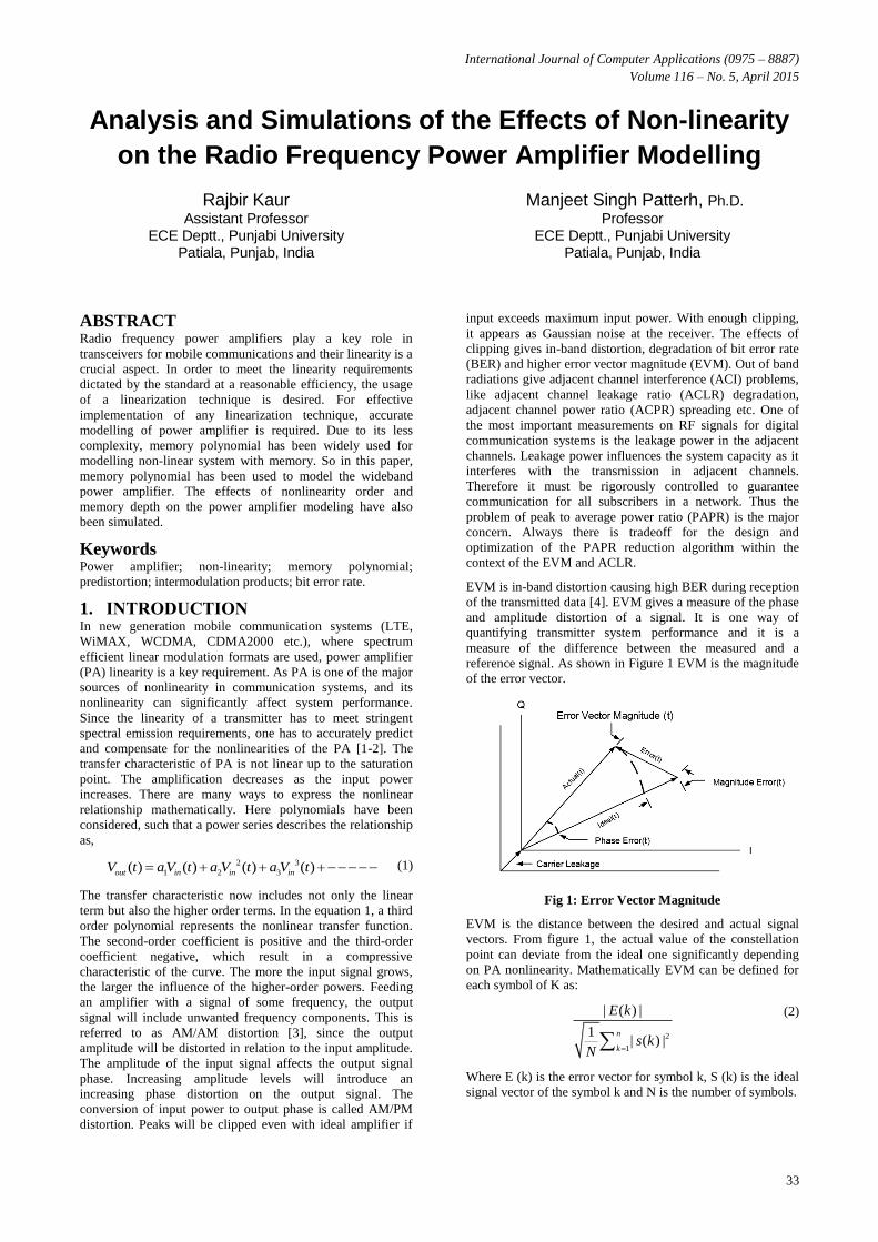
EVM is in-band distortion causing high BER during reception

of the transmitted data [4]. EVM gives a measure of the phase

and amplitude distortion of a signal. It is one way of

quantifying transmitter system performance and it is a

measure of the difference between the measured and a

reference signal. As shown in Figure 1 EVM is the magnitude

of the error vector.

Fig 1: Error Vector Magnitude

EVM is the distance between the desired and actual signal

vectors. From figure 1, the actual value of the constellation

point can deviate from the ideal one significantly depending

on PA nonlinearity. Mathematically EVM can be defined for

each symbol of K as:

2

1

| ( ) |

1| ( ) |

n

k

E k

s kN

(2)

Where E (k) is the error vector for symbol k, S (k) is the ideal

signal vector of the symbol k and N is the number of symbols.



34

Therefore some linearization techniques are required to

minimize the distortion on the transmit signal. Among all the

linearization techniques, digital predistortion (DPD) is the

most efficient and cost effective technique [5]. Memory

polynomial PA model is a simplified model based on indirect

learning architecture. This model is able to capture some of

the memory effects, while reducing the number of parameters

describing the model. Proposed memory polynomial model

can be used for any wideband PA data. In this paper for

modelling PA, the degree and order of memory polynomial

can be varied to obtain the optimum result. The paper is

organized as follows: section I provides the introduction to

PA and non-linearity problem in PA, section II gives

nonlinearity analysis of PA using Single-tone stimulus and

Two-Tone stimulus analysis, section III gives memory

polynomial model using indirect learning architecture, section

IV gives the results for memory polynomial model and

section V concludes the paper.

2. NON-LINEARITY IN POWER

AMPLIFIER Memory Polynomial model for power amplifier shows the

non-linearity with memory effects [6]. This model can be

designed with unity time delay taps and also with non-

uniform time delay taps. Modelling is done by using data in

discrete time domain. Signal is first converted from

continuous to discrete by a method of sampling. If ( )V tin is

the input signal to the sampler, then the output of sampler is:

( ) ( . )V i V i Tout in , Where T is the sampling period and

sampling frequency is1

FsamplesT

.

Let the baseband signal is

( ) ( ). ( ( )in cZ t V t Cos t t

(3)

Here c is the angular carrier frequency, V(t) is the amplitude

and ( )t is the phase of the signal. The envelop band width of

this signal is much lower than the carrier frequency. This

signal can be written in terms of in-phase and quadrature

components as:

( ) ( ). ( ) ( ).sin( )in c cZ t I t Cos t Q t t (4)

Where ( ) ( ). ( )I t V t Cos t

( ) ( ). ( )Q t V t Sin t (5)

Equation (4) can be re-written in complex form as:

( ) ( ). ( ) . ( ) ( ). ( ) .sin( )in c cZ t V t Cos t Cos t V t Sin t t (6)

( ) Re ( ). cj t

inZ t A t e (7)

Here ( )A t is a base band signal and

( )( ) ( ). j tA t V t e

(8)

2.1 Nonlinearity Analysis of Power

Amplifier using Single-Tone Stimulus For a linear amplifier the output can be described as:

( ) . ( )o Lin inZ t G Z t (9)

where GLin is a time independent linear amplifier gain.

Practically due to non-linearity, the output of amplifier

saturates at some value as the input signal amplitude is

increased. Due to non-linearity, amplifier has a non-constant

gain and non-linear phase. These amplifiers are called quasi-

memory-less amplifiers and described by the polynomial as

0

( ) . ( )K

k

o k in

k

Z t a Z t

(10)

2

0 1 2( ) . ( ) . ( ) . ( )k

o in in k inZ t a a Z t a Z t a Z t (11)

In equation (11), k is the maximum polynomial order which

shows the non-linearity of the amplifier.

, ,0 1 2a a a ak are complex polynomial coefficients,

which determine the exact shape of the input-out-put

characteristics. For memory-less case, these polynomials are

real values. By using trigonometric formulas, the quasi-

memory-less amplifier will produce new frequency

components which are located at the harmonics (

2 , 3 , K ) of the input signal.

From equation (7)

( ) ( ). ( )in cZ t V t Cos t t (12)

By substituting this value in equation 10,

0

( ) . ( ). ( ( ))K

k

o k c

k

Z t a V t Cos t t

(13)

When time constant of the amplifier is very small compared to

the amplitude ( )V t and phase ( )t , then for narrow band

application i.e <1.2 MHz, these amplitude and phase

variations can be neglected and assuming it to be constant [7],

But for high memory amplifiers it comes in the form of

memory effects. Memory effects can be described as changes

in the amplitude and phase of the output signal as function of

the input signal amplitude and can be expressed as

0 ) )( ) ( .cos (o in c out inZ t V V t V (14)

Whose complex envelop will be

)(

)( ) ( . out inj V

out out inA t V V e

(15)

This AM/AM conversion is used to evaluate the 1-db

compression point.

2.2 Nonlinearity of Power Amplifier in

Two-Tone Analysis Let the two-tone input signal to the power amplifier is

1 2( ) cos ( ) cos ( )in in inZ t V t V t (16)

1 2 , 2 1



35

2 1 2 1( ) 2 cos( ).cos( )2 2

in inZ t V t t

(17)

Here frequency2 1

( )

2

is the modulating frequency m ,

which is half of the frequency spacing between two tones.

2 1( )

2

t

is the RF center frequency. So equation (17) can

be written as:

( ) 2 cos( ).cos( )in in m cenZ t V t t (18)

This two tone signal is recognized as double sideband

suppressed carrier signal having carrier frequency cen and

modulating frequency m . When this signal is applied to PA,

the output signal can be expressed as:

1 2

0

( ) . ( ). ( )cosK

k

o k

k

Z t a V t Cos t V t t

(19)

By expanding equation (19), new frequency components will

appear, which shows the non-linearity of the device and called

inter-modulation distortion [7]. In two-tone signal these are

computed as:

1 2. .new (20)

Where and are positive integers including zero.

k denotes the order of the inter-modulation distortion.

To examine inter-modulation products, two frequencies 1

and 2 , some of the orders of intermodulation products have

been considered. To define the order, harmonic multiplying

constants have been added with two frequencies producing the

inter-modulation product. For example ( 1 2 ) is second

order, ( 2 1 2 ) is third order, ( 3 21 2 ) is fifth order,

& so on. For 1 and 2 to be two frequencies of 200 kHz

and 201 kHz which are 1 kHz apart, table 1 is showing the

inter-modulation products.

Table 1-Intermodulation products

Order Freq. 1 Freq. 2 Freq. 1

(kHz)

Freq. 2

(kHz)

First ω1 ω2 200 201

Second ω1 + ω2 ω2 - ω1 401 1

Third 2ω1 - ω2 2ω2 - ω1 199 202

Fourth

2ω1 + ω2 2ω2 + ω1 601 602

2ω1 + ω2 2ω2 - 2ω1 802 2

Fifth

3ω1 - ω2 3ω2 - 2ω1 198 203

3ω1 + 2ω2 3ω2 + 2ω1 1002 1003

From table 2, only the odd order inter-modulation products

are close to the two fundamental frequencies 1 and 2 . One

third order product (2 )1 2 is 1 kHz lower in frequency

than 1 and another third order product (2 )2 1 is 1 kHz

above 2 . One fifth order product (3 2 )1 2 is 2 kHz

below 1 and another (3 2 )2 1 is 2 kHz above 2 .

Table 2-Odd order products

Order Freq. 1 Freq. 2 Freq. 1

(kHz)

Freq. 2

(kHz)

Third 2ω1 - ω2 2ω2 - ω1 199 202

Fifth 3ω1 - ω2 3ω2 - 2ω1 198 203

Seventh 4ω1 - 3ω2 4ω2 - 3ω1 197 204

Ninth 5ω1 - 4ω2 5ω2 - 4ω1 196 205

In fact the odd order products are closest to the fundamental

frequencies 1 and 2 . The in-band IMD products cannot be

easily filtered out [8]. The most commonly used measure of

IMD is the ratio of the largest IMD (almost third order IMD)

to the one of the two tone. For complex input signals non-

linearity appears over a continuous band of frequencies and is

referred as spectral regrowth.

3. INDIRECT LEARNING

ARCHITECTURE The basic algorithm taken for this work is memory

polynomial model. There are two methods to extract the

power amplifier coefficients. One method is to model the

power amplifier and then find its inverse. Since memory

effects are also considered, so it is not possible to extract the

exact inverse of the non-linear system. Second method is to

use indirect learning architecture directly because it eliminates

the assumptions about the model parameter estimation of the

PA. The general form of a baseband memory polynomial PA

model can be written as:

2 1

0 1

. ( )Q K

k

out kq n

q k

Z n W x n q

(21)

where Wkqare complex memory polynomial coefficients. An

integer value is given to k as k=0, 1, 2, 3----K. xn and

Z nout are the measured discrete input and output complex

envelope signals of nth sample. q = 0,1,2,3-----Q is the

memory interval and equal to sampling interval T. Q is the

maximum memory and K is the maximum polynomial order

[9]. Since even terms are far away from the center frequency,

only odd terms are considered.

Let

2 1( ) ( ) k

kq nU n q x n q (22)

By substituting equation (22) in equation (21),



36

0 1

( )Q K

out kq kq

q k

Z n W U n q

(23)

Let

1

( )K

q kq kq

k

U W U n q

(24)

By using equation (22)

2 1

1

( )K

k

q kq n

k

U W x n q

(25)

After substituting this value in equation (23),

0

( )Q

out q

q

Z n U n q

(26)

Equation (21) can be represented as memory polynomial

model with unity delay taps as shown in figure 2. The unity

delay taps are denoted by the symbol1

Z

. When 1

Z

delay

tap is applied to the sequence of discrete digital values [10-

11]; the tap gives the previous value in the sequence and

introduces a delay of one sampling interval q. Apply the value1

Z

to the input value xn gives the previous input 1x nn .

Fig 2: Memory Polynomial Model with Unity Delay

1 ( ) 1nZ x x n q x n (27)

Substitute value of q in equation (23)

0 0 1 1

1 1

1

( ) ( 1) ....

( )

K K

out k k k k

k k

K

kQ kQ

k

Z n W U n W U n

W U n Q

(28)

0 1 2out QZ n U U U U

(29)

By substituting values of k & q in equation (23),

10 10 20 20

0 0 11 11 21 21

1 1

1 1 2 2

( ) ( ) .....

( ) ( ) ( ) .....

( 1) .....

( ) ( ) ....

( )

out

k k

k k

Q Q Q Q

kQ kQ

Z n W U n W U n

W U n W U n W U n

W U n

W U n W U n

W U n Q

(30)

Equation (30) can be written in matrix form as

.outZ U W (31)

Where

0 , 1 , 2 1T

out out out out outZ Z Z Z Z n (32)

10 20 0

11 21 1,

1 2 ,

, , ,

, , ,

, ,

T

k

k

Q Q kQ

W W W

W W WW

W W W

10 20 0

11 21 1,

1 2 ,

, , ,

, , ,

, ,

k

k

Q Q kQ

U U U

U U UU

U U U

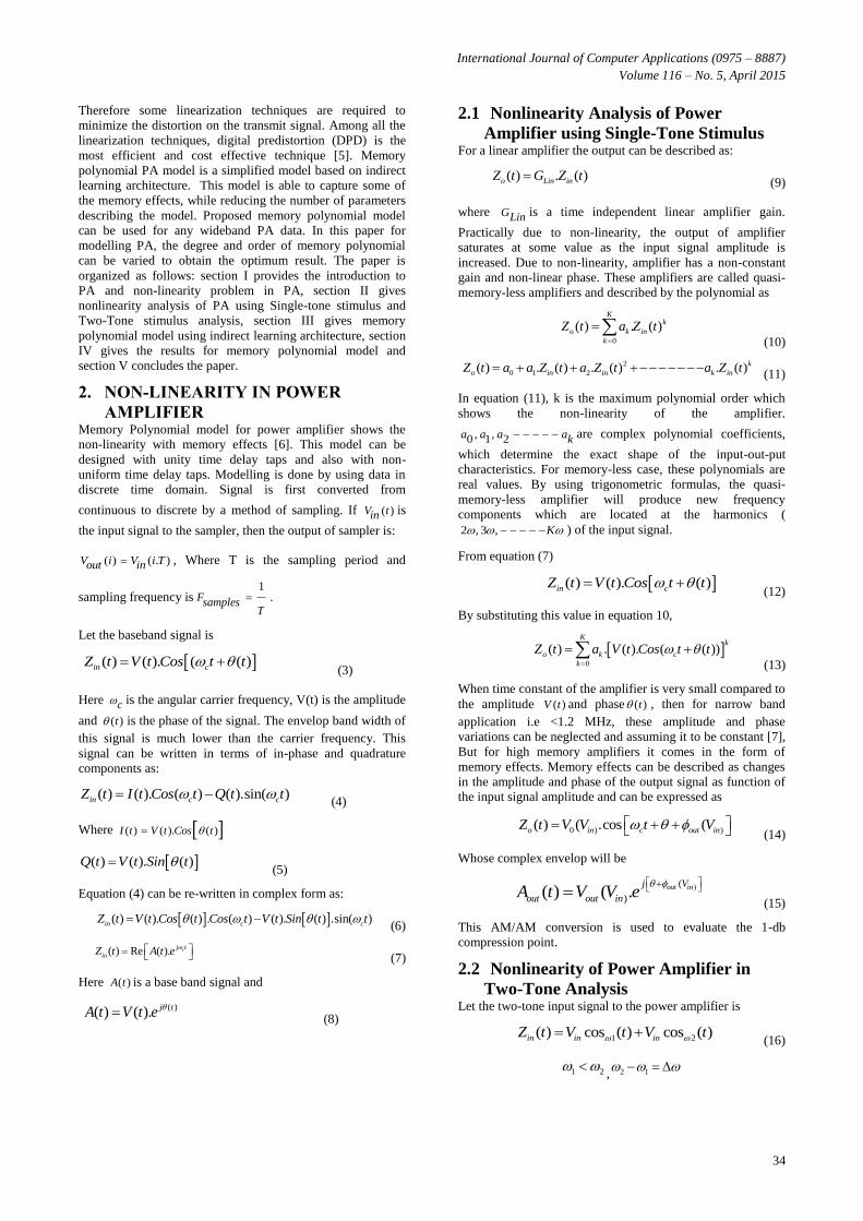
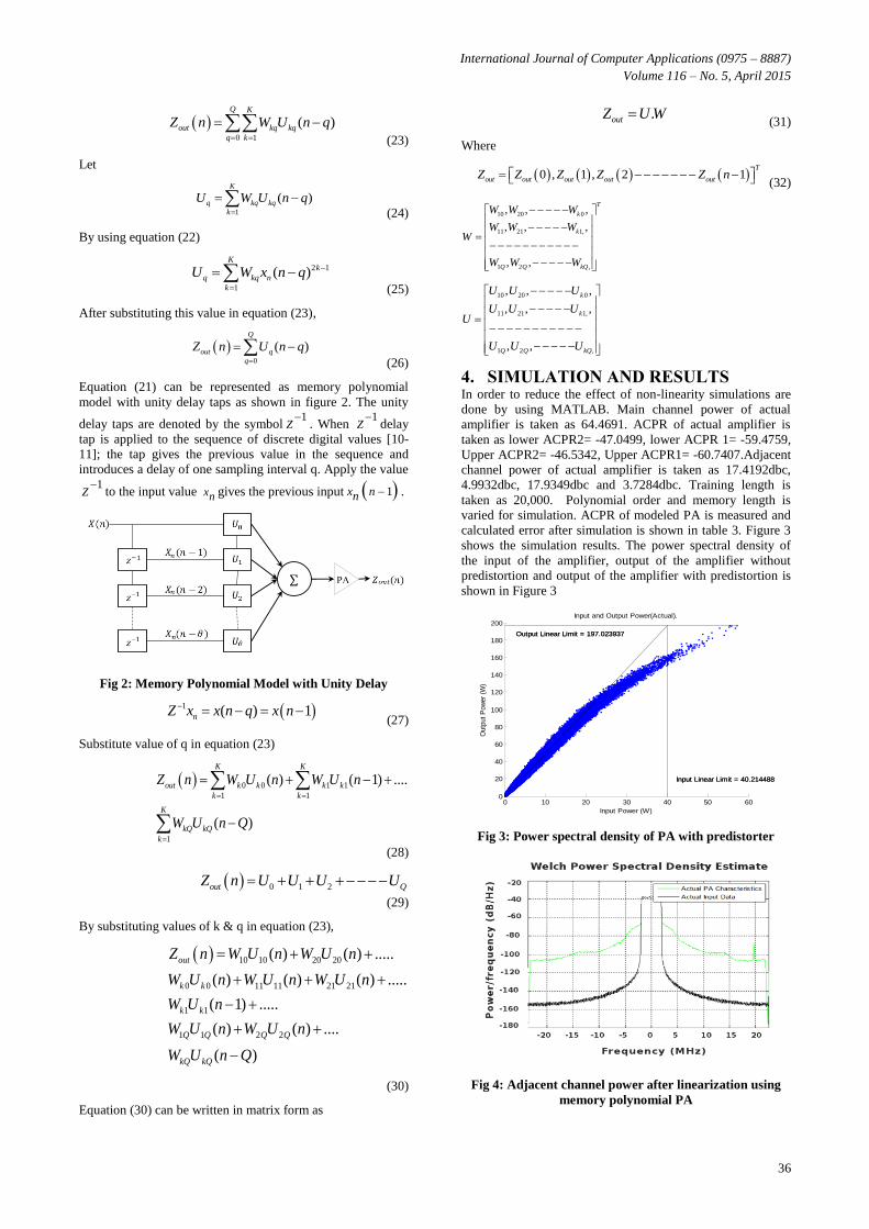
4. SIMULATION AND RESULTS In order to reduce the effect of non-linearity simulations are

done by using MATLAB. Main channel power of actual

amplifier is taken as 64.4691. ACPR of actual amplifier is

taken as lower ACPR2= -47.0499, lower ACPR 1= -59.4759,

Upper ACPR2= -46.5342, Upper ACPR1= -60.7407.Adjacent

channel power of actual amplifier is taken as 17.4192dbc,

4.9932dbc, 17.9349dbc and 3.7284dbc. Training length is

taken as 20,000. Polynomial order and memory length is

varied for simulation. ACPR of modeled PA is measured and

calculated error after simulation is shown in table 3. Figure 3

shows the simulation results. The power spectral density of

the input of the amplifier, output of the amplifier without

predistortion and output of the amplifier with predistortion is

shown in Figure 3

Fig 3: Power spectral density of PA with predistorter

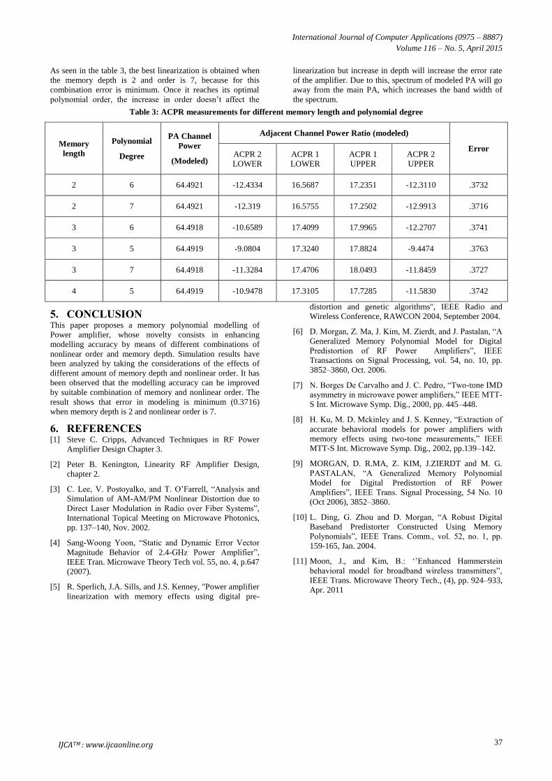
Fig 4: Adjacent channel power after linearization using

memory polynomial PA

0 10 20 30 40 50 600

20

40

60

80

100

120

140

160

180

200Input and Output Power(Actual).

Input Power (W)

Outp

ut

Pow

er

(W)

Input Linear Limit = 40.214488

Output Linear Limit = 197.023937

Input Linear Limit = 40.214488

Output Linear Limit = 197.023937



37

As seen in the table 3, the best linearization is obtained when

the memory depth is 2 and order is 7, because for this

combination error is minimum. Once it reaches its optimal

polynomial order, the increase in order doesn‟t affect the

linearization but increase in depth will increase the error rate

of the amplifier. Due to this, spectrum of modeled PA will go

away from the main PA, which increases the band width of

the spectrum.

Table 3: ACPR measurements for different memory length and polynomial degree

Memory

length

Polynomial

Degree

PA Channel

Power

(Modeled)

Adjacent Channel Power Ratio (modeled)

Error ACPR 2

LOWER

ACPR 1

LOWER

ACPR 1

UPPER

ACPR 2

UPPER

2 6 64.4921 -12.4334 16.5687 17.2351 -12.3110 .3732

2 7 64.4921 -12.319 16.5755 17.2502 -12.9913 .3716

3 6 64.4918 -10.6589 17.4099 17.9965 -12.2707 .3741

3 5 64.4919 -9.0804 17.3240 17.8824 -9.4474 .3763

3 7 64.4918 -11.3284 17.4706 18.0493 -11.8459 .3727

4 5 64.4919 -10.9478 17.3105 17.7285 -11.5830 .3742

5. CONCLUSION This paper proposes a memory polynomial modelling of

Power amplifier, whose novelty consists in enhancing

modelling accuracy by means of different combinations of

nonlinear order and memory depth. Simulation results have

been analyzed by taking the considerations of the effects of

different amount of memory depth and nonlinear order. It has

been observed that the modelling accuracy can be improved

by suitable combination of memory and nonlinear order. The

result shows that error in modeling is minimum (0.3716)

when memory depth is 2 and nonlinear order is 7.

6. REFERENCES [1] Steve C. Cripps, Advanced Techniques in RF Power

Amplifier Design Chapter 3.

[2] Peter B. Kenington, Linearity RF Amplifier Design,

chapter 2.

[3] C. Lee, V. Postoyalko, and T. O‟Farrell, “Analysis and

Simulation of AM-AM/PM Nonlinear Distortion due to

Direct Laser Modulation in Radio over Fiber Systems”,

International Topical Meeting on Microwave Photonics,

pp. 137–140, Nov. 2002.

[4] Sang-Woong Yoon, “Static and Dynamic Error Vector

Magnitude Behavior of 2.4-GHz Power Amplifier”,

IEEE Tran. Microwave Theory Tech vol. 55, no. 4, p.647

(2007).

[5] R. Sperlich, J.A. Sills, and J.S. Kenney, "Power amplifier

linearization with memory effects using digital pre-

distortion and genetic algorithms", IEEE Radio and

Wireless Conference, RAWCON 2004, September 2004.

[6] D. Morgan, Z. Ma, J. Kim, M. Zierdt, and J. Pastalan, “A

Generalized Memory Polynomial Model for Digital

Predistortion of RF Power Amplifiers”, IEEE

Transactions on Signal Processing, vol. 54, no. 10, pp.

3852–3860, Oct. 2006.

[7] N. Borges De Carvalho and J. C. Pedro, “Two-tone IMD

asymmetry in microwave power amplifiers,” IEEE MTT-

S Int. Microwave Symp. Dig., 2000, pp. 445–448.

[8] H. Ku, M. D. Mckinley and J. S. Kenney, “Extraction of

accurate behavioral models for power amplifiers with

memory effects using two-tone measurements,” IEEE

MTT-S Int. Microwave Symp. Dig., 2002, pp.139–142.

[9] MORGAN, D. R.MA, Z. KIM, J.ZIERDT and M. G.

PASTALAN, “A Generalized Memory Polynomial

Model for Digital Predistortion of RF Power

Amplifiers”, IEEE Trans. Signal Processing, 54 No. 10

(Oct 2006), 3852–3860.

[10] L. Ding, G. Zhou and D. Morgan, “A Robust Digital

Baseband Predistorter Constructed Using Memory

Polynomials”, IEEE Trans. Comm., vol. 52, no. 1, pp.

159-165, Jan. 2004.

[11] Moon, J., and Kim, B.: „‟Enhanced Hammerstein

behavioral model for broadband wireless transmitters”,

IEEE Trans. Microwave Theory Tech., (4), pp. 924–933,

Apr. 2011

IJCATM : www.ijcaonline.org

Documents

Analysis and Simulations of the Effects of Non-linearity