I /~ / .--

\ .; I . !

(

i:

!',

J.

SOUTHWEST RESEARCH INSTITUTE Po~t Office Drawer 28510, 6220 Culebra Road

San Antonio, Texas 78284

~;.s~rl r\Jf)

!~- ()OW I) IN f.

t~ ('C'

c

Analysis and Testing of Pipe Response to Buried Explosive Detonations

by PeterS. Westine

Edward D. Esparza

Alex B. Wenzel

for The Pipeline Research Committee

American Gas Association

.July 1978

Approved:

' H. Norn~an Abramson, Vice President

Engineering Scier~ces Division

'·

I

i /

/

ACKNOVJLEDC::HENTS

This program was sponsored by the Pipeline Research Committee of the

American Gas Association and conducted by Southwest Research Institute.

The authors thank the supervisory committee for their guidance and direction,

suggestionst and cooperation during the conduct of the program. Members of

this committee are:

Mr. Osborne Lucas - Chairman, Columbia Gas Transmission Corp.

Mr. J. M. Holden, American Gas Association

Mr. J. S. Taylor, Consumers Power Company

Mr. J. D. McNorgant Southern California Gas Company

Mr. R. L. Penning, Panhandle Eastern Pipe Line Company

Mr. C. P. Hendrickson, Northern Illinois Gas Company

Mr. H. E. Russell, Transcontinental Gas Pipe Line Corp.

Mr. J. T. Sickman, Texas Eastern Transmission Corp.

Mr. G. J. Bart, Texas Gas Transmission Corp.

In addition, the authors are very grateful for the support, assistance and

cooperation provided by Panhandle Eastern Pipe Line Co.t and the Texas Gas

Transmission Corp. in conducting the field experiments at the Kansas City

and Kentucky remote test sites respectively. Furthermore, funding of

part of this program was also provided by Texas Gas Transmission Corp. to

conduct the field experiments at the Kentucky site.

At Southwest Research Institute the authors are especially indebted

to the following personnel:

Messrs. E. R. Garcia, Jr. and A. C. Garcia - for performing the

field experiments

Dr. W. E. Baker - technical consultation and review of analysis

Mr. J. J. Kulesz -assistance in conducting the model experiments

Mr. R. A. Cervantes - assistance in performing model experiments

Mr. J. C. Hokanson- programming of data reduction codes

Mses. T~ K. Moseleyt P. A. Huggt andY. R. Martinez- data reduction

Mr. V. J. Hernandez - final drawing of illustrations

iii

I Mmes E. Hernandez, J. Cooke and C. W. Dean- typing of interim and

final reports.

Ms. D. J. Stowitts, - for editing and proofing the final report.

The assistance and cooperation of these individuals is greatly appreciated.

iv

,.,t

•,. I

,,

j I'

EXECUTIVE SUMMARY

This final report describes experimental tests and analytical solutions

in a research program to develop procedures for predicting the maximum cir­

cumferential and longitudinal stresses in pipelines caused by nearby buried

explosive detonations. This study was conducted over a period of 2.5 years

by Southwest Research Institute for the Pipeline Research Committee of the

American Gas Association.

The approach followed in developing a final solution evolved from a

combination of experimental and theoretical studies, specifically:

• Similitude theory

• Model tests on small buried pipes

• Approximate energy procedures based on assumed deformed

pipe shapes

• Conservation of mass and momentum principles for shock fronts

• Empirical observation based on past investigations

• Full scale experimental data generated during this study.

To develop this final relationship for predicting pipe stresses, the

problem was divided into two parts. The first problem was to estimate the

maximum soil particle velocities and displacements at various distances from

either buried single detonations (point sources) or multiple detonations (line

sources) . These ground motions provide the forcing function imparted to the

buried pipe. The second problem was to estimate both maximum circumferential

and longitudinal stresses in buried pipe caused by these maximum ground mo­

tions. After the results of the first solution were substituted into the

results of the second solution, pipe stress solutions for circumferential

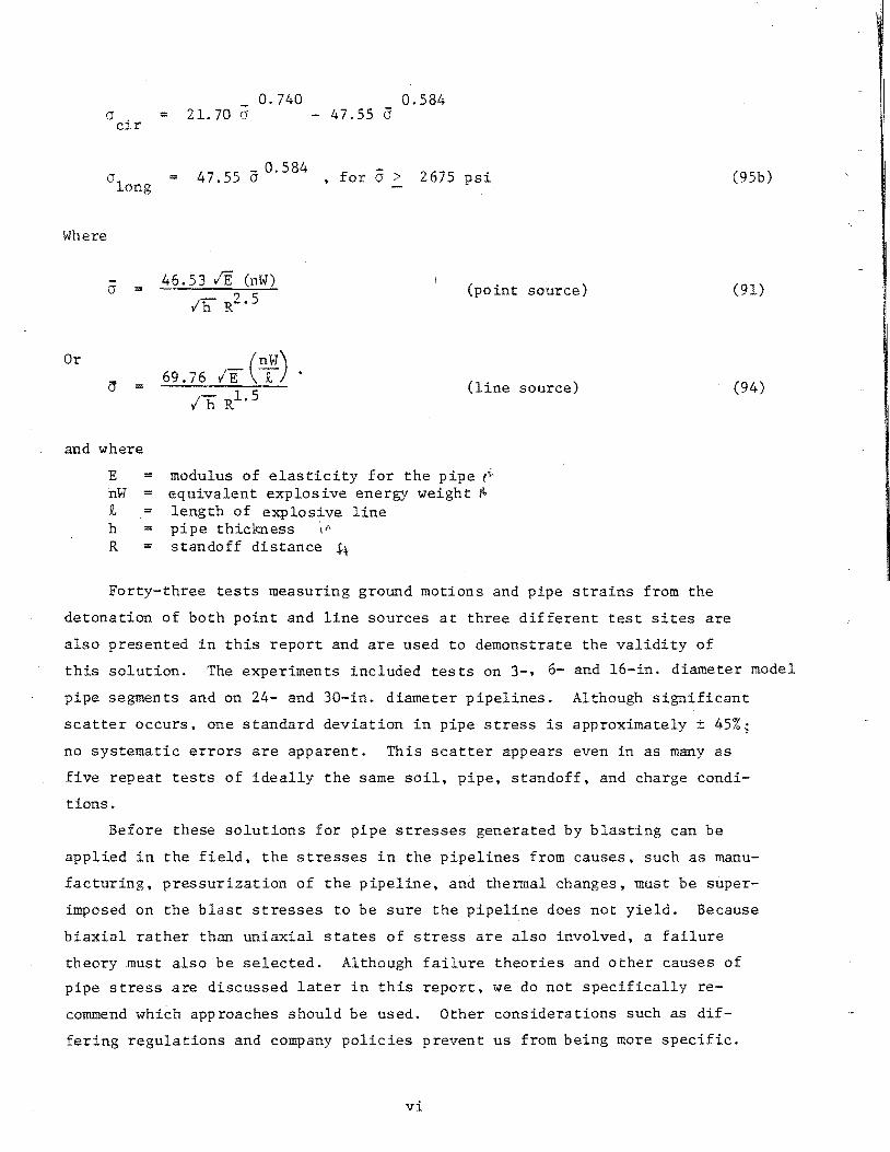
stress cr • and longitudinal stress a1

were obtained and computed from c1r · ong · the equations:

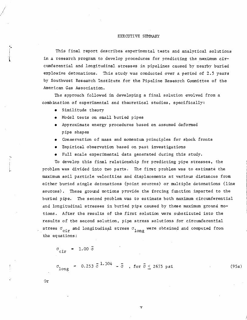
-a . = 1. 00 a c1r

a = long o. 25 3 a 1. 304 - 0 • for a < 2675 psi (95a)

Or

v

a cir

a long

Where

a =

Or

(j =

and where

E = n~T = ~

h = R

- o. 740 0.584 = 21.70 a - 47,55 0

47.55 - 0. 584 for > 2675 psi = a , a

46.53 IE (nW) (point source)

/h R2.5

(n~T) 69.76 IE" T

/h Rl.S (line source)

modulus of elasticity for the pipe ri· equivalent explosive energy weight 1.1.

length of explosive line pipe thickness ·," standoff distance S-t

Forty-three tests measuring ground motions and pipe strains from the

detonation of both point and line sources at three different test sites are

also presented in this report and are used to demonstrate the validity of

(95b)

(91)

(94)

this solution. The experiments included tests on 3-, 6- and 16-in. diameter model

pipe segments and on 24- and 30-in. diameter pipelines. Although significant

scatter occurs, one standard deviation in pipe stress is approximately ± 45% .;

no systematic errors are apparent. This scatter appears even in as many as

five repeat tests of ideally the same soil, pipe, standoff, and charge condi­

tions.

Before these solutions for pipe stresses generated by blasting can be

applied in the field, the stresses in the pipelines from causes, such as manu­

facturing, pressurization of the pipeline, and thermal changes, must be super­

imposed on the blast stresses to be sure the pipeline does not yield. Because

biaxial rather than uniaxial states of stress are also involved, a failure

theory must also be selected. Although failure theories and other causes of

pipe stress are discussed later in this report, we do not specifically re­

commend which approaches should be used. Other considerations such as dif­

fering regulations and company policies prevent us from being more specific.

vi

..

These factors eventually will require each pipeline company to use this re­

search report only as a guide in writing their individual corporate procedures

for determining how close to their pipelines blasting can be conducted.

This report is a research report and not a field manual. To help guide

corporate development of an appropriate field manual. we present six alter­

nate ,;.;ays that these equations ca.n be presented, illustrated, and discussed

for possible use in field manuals. Tables, nomographs, and figures are

used to illustrate different approaches which might be considered in decid­

ing which technique is easier for personnel to apply in computing pipe stresses

from blasting.

A sensitivity analysis was also conducted which indicated that pipe

stresses from blasting are most sensitive to standoff distance Rand least/

sensitive to the modulus of elasticity of the pipe E and pipe thickness h.

Surprisingly, the pipe stresses are independent of the soil density p • the -~~-~---~------~~---- ~ ~-~ ~~ ~ ~------~-~ ~ . ---~-~~-----~~-~----~- -~---- ~----- -- ---~- ~- . s----

soil seismic propagation velocity c, and the pipe diameter D. The mathema-/..-...----------·--·-··-·-··,~···. ··- ·- .

tics of the solution must be studied to understand why these parameters fall

out of the analysis. The experimental tests also verified these observations.

Dynamic analysis procedures and not static ones must be used to understand

these or other conclusions.

As with any analysis procedure, this solution is based upon assumptions

which limit its applicability. Three considerations for additional work are

suggested in the conclusions and recommendations which could lead to an im­

proved solution. The most important of these is that the explosive is

idealized as either a point or a line source. Most problems which will be

encountered in the field come from the detonation of an explosive grid .. More

model tests in this area would be beneficial. Until this work is performed,

engineering judgment will be required in order to apply these results to

field conditions.

vii

•,

..

Figure

1

2

3

4

5

6

7

8

9

10

11

12

13

14

15

16

17

18

19

20

21

22

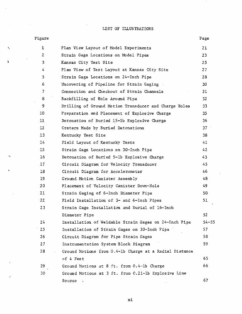
LIST OF ILLUSTRATIONS

Plan View Layout of Model Experiments

Strain Gage Locations on MOdel Pipes

Kansas City Test Site

Plan View of Test Layout at Kansas City Site

Strain Gage Locations on 24-Inch Pipe

Uncovering of Pipeline for Strain Gaging

Connection and Checkout of Strain Channels

Backfilling of Hole Around Pipe

Drilling of Ground Motion Transducer and Charge Holes

Preparation and Placement of Explosive Charge

Detonation of Buried 15-lb Explosive Charge

Craters Made by Buried Detonations

Kentucky Test Site

Field Layout of Kentucky Tests

Strain Gage Locations on 30-Inch Pipe

Detonation of Buried 5-lb Explosive Charge

Circuit Diagram for Velocity Transducer

Circuit Diagram for Accelerometer

Ground Motion Canister Assembly

Placement of Velocity Canister Down-Hole

Strain Gaging of 6-Inch Diameter Pipe

Field Installation of 3- and 6-Inch Pipes

23 Strain Gage Installation and Burial of 16-Inch

Diameter Pipe

24

25

26

27

28

29

Installation of Weldable Strain Gages on 24-Inch Pipe

Installation of Strain Gages on 30-Inch Pipe

Circuit Diagram for Pipe Strain Gages

Instrumentation System·Block Diagram

Ground Motions from 0.4-lb Charge at a Radial Distance

of 4 Feet

Ground Motions at 8 ft. from 0.4-lb Charge

30 Ground Motions at 3 ft. from 0.21-lb Explosive Line

Source

xi

Page

21

23

25

27

28

30

31

32

33

35

36

37

38

41

42

43

45

46

48

49

50

51

52

54-55

57

58

59

65

66

67

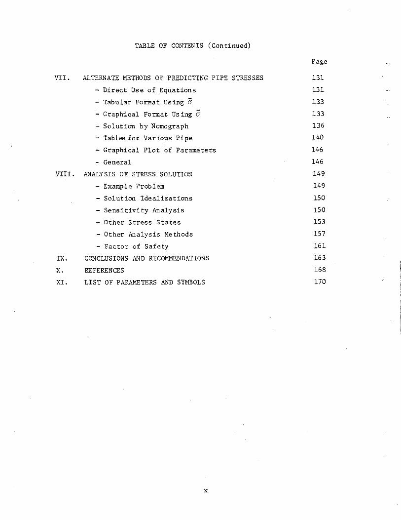
TABLE OF CONTENTS (Continued)

VII. ALTERNATE METHODS OF PREDICTING PIPE STRESSES

- Direct Use of Equations

Tabular Format Using a - Graphical Format Using a - Solution by Nomograph

- Tables for Various Pipe

- Graphical Plot of Parameters

- General

VIII. ANALYSIS OF STRESS SOLUTION

- Example Problem

IX.

X.

XI.

- Solution Idealizations

- Sensitivity Analysis

- Other Stress States

- Other Analysis Methods

- Factor of Safety

CONCLUSIONS AND RECOMMENDATIONS

REFERENCES

LIST OF PARAMETERS AND SYMBOLS

X

Page

131

131

133

133

136

140

146

146

149

149

150

150

153

157

161

163

168

170

Figure

31

32

33

34

35

36

37

38

39

40

41

42

43

44

45

LIST OF ILLUSTRATIONS (Continued)

Horizontal Velocities from 0.05-lb. Charge

Radial Ground Motions at 12 ft. from 15-lb. Charge

Radial Soil Motions at 12 ft. from a 5-lb Charge

Radial Soil Motions at 12 ft. from a 5-lb. Charge

Radial Soil Motions at 12 ft. from a 3-lb Charge

Circumferential Strain Measurements on 3-Inch

Diameter Pipe

Strain Measurements for 6-Inch Pipe

Blast Strain Records for 24-Inch Pipe

Test No. 6 Blast Strains on 24-Inch Pipe

Test No. 6 Blast and Internal Pressure Strains on

24-Inch Pipe

Test No. 4 Strains on 30-Inch Pipe

Ground Displacement in Rock and Soil No Coupling

Particle Velocity in Rock and Soil No Coupling

Coupled Displacement in Rock and Soil

Coupled Particle Velocity in Rock and Soil

46 Radial Soil Displacement from Line Charge

Detonations

47 Maximum Soil Particle Velocity from Line Charge

Detonations

48

49

50

51

52

53

•54

55

56

57

58

59

60

Equation 46 Compared to Displacement Test Data

Assumed Distribution of Impulse Imparted to a Pipe

Circumferential Pipe Stress

Longitudinal Pipe Stress

Graphical Solution Using a

Pipe Stress Nomograph for Point Sources

Pipe Stress Nomograph for Line Sources

Graphical Plot of Blasting Pipe Stresses

Plan View of an Example Field Blasting Problem

Stress States for Different Yield Theories

Simplified Yield Theories

Qualitative Ground Shock Model

Battelle Circumferential Stress Formula

xii

Page

68

71

72

75

76

78-79

80-81

85-86

87-88

89-90

93-94

100

102

105

106

109

110

112

115

125

128

135

137

138

147

151

155

156

157

160

'·

/',

Table

I

II

III

IV

v

VI

VII

VIII

IX

X

XI

XII

XIII

XIV

XV

XVI

XVII

XVIII

XIX

XX

LIST OF TABLES

Scale Factors for a Replica Modeling Law

Summary of Test Conditions for Model Experiments

Tests Conducted at Kansas City Test Site

Kentucky Tests

Summary of Horizontal Ground Motion Data from Model

Tests

Radial Soil Motion Data from Kansas City Tests

Ground Notion Data

Maximum·Strains from Model Experiments

Maximum Blast Pipe Stresses for Model Test

Maximum Strains from Blast Loading on 24-Inch Pipe

Combined Blast and Internal Pressure Strains

Maximum Blast Stresses on 24-Inch Pipe

Maximum Blast Strains Measured on 30-Inch Pipe

Maximum Blast Stresses in 30-Inch Pipe

Measured Durations and Computer Periods

Equivalent Energy Release

Stresses in Pipes from Blasting

Stress in Buried Pipe from Point Source Blasting

Stresses Used in Extrapolation

Results of Sensitivity Analysis

xiii

Page

15

20

26

39

63

70

73

82

83

91

91

91

95

95

118

129

134

141-144

145

152

\

'·

,.

I. INTRODUCTION

This final report describes a research program to develop functional

relationships for predicting the stress in pipelines caused by nearby blast­

ing. This program was conducted during the period of 1975 through 1977 by

Southwest Research Institute (SwRI) for the Pipeline Research Committee of

the American Gas Association (A.G.A.), under Project No. PR 15-76 . . To accomplish the above objective, the program was divided and funded

in three phases which had several tasks in each phase. The Phase I effort

to formulate an analysis procedure included tasks to:

• Review the literature on ground shock propagation and effects of shock

loading on buried pipe-like structures; and

• Qualitatively plan an analytical approach and limited test program for

predicting the change in pipe stresses from buried detonations.

The Phase II effort to conduct limited experiments to generate the necessary

data for developing a solution included tasks to:

• Quantify procedures for estimating the loads on pipes from both single

sourc~ and multi-source buried detonations;

• Quantify procedures for predicting the maximum dynamic circumferential

and longitudinal stresses in pipe from blast loads; and

• Use model tests on various pipe to experimentally generate and validate

the ground shock and pipe stress solutions.

The Phase III effort to validate the solution by conducting actual pipeline

tests included tasks to:

• Conduct several field evaluations by measuring additional stresses and

ground motions at actual pipeline sites to enhance the solution and

demonstrate its validity;

• Present alternate methods for the pipeline industry to use the result­

ing stress from blasting solution; and

• Complete an engineering report on these efforts.

The resulting solution interrelates type of explosive, amount of explo­

sive, standoff distance, pipe size, pipe properties, and the resultant

lon tudinal and circumferential pipe stresses caused by blasting. In order

to create such a solution. the general problem had to be divided into two

separate parts. The first part estimated maximum particle velocity and

maximum soil displacement at various distances from either single detonations

(point sources) or multiple detonations (line sources). The second problem

was then the estimate of both circumferential and longitudinal maximum dyna­

mic pipe stresses caused by the previously determined maximum ground motions.

This division of the general problem into these two separate parts is apparent

throughout the report until such time as the solutions are combined to give

a final interre}ationship.

The solution which finally evolved is in an explicit closed form which

can be solved using graphs, tables, or a hand calculator. To accomplish this

task, similitude theory had to be combined with theoretical approaches using

energy procedures, conservation of mass and momentum principles for shock

fronts, and empirical observation before a final solution evolved. The ground

shock propagation problem was solved by using similitude theory to create pi

terms, empirical observation to combine two of these pi terms, and a vast

quantity of test data from both the literature and tests conducted in this

study to interrelate scaled energy release and standoff distance to scaled

ground motion. The ground motion solution which results from this effort

works for small energy releases such as 0.03 lbs. of explosive to large

kiloton nuclear blasts. Peak particle displacement predicted from this solu­

tion is then combined with the Hugoniot equations for conservation of mass

and momentum to estimate the impulse imparted to a buried pipeline. Finally,

assumed deformed shapes, a conservation of energy solution, and empirical

observation using measured strains on actual buried pipe segments are used

to develop the final stress solution.

Forty-three tests measuring ground motions and pipe strains from the

detonation of both point and line sources at three different test sites are

also described. These experiments include tests on 3-, 6- and 16-in. dia­

meter model pipe segments as well as experiments on actual 24- and 30-in.

diameter pipelines. The test results are used to both develop the previous­

ly mentioned ground motion and pipe stress solutions and demonstrate the

validity of the resulting analyses.

This report is organized into eleven sections, Section II describes the

analytical basis using similitude theory for the design of the experiments.

The model analysis presented in this section concentrates on developing func­

tional relationsh.ips to determine 1) soil particle velocity and displacement

2

..

,.

for both a point and line explosive source, and 2) pipe stresses caused by

these ground motions. The purpose of this section is to show why model

tests could be used in place of full-scale prototype experiments to accumu­

late the major quantity of test data.

Section III describes the test sites, the experiments performed at each

site. and measurement systems used. Model tests using 3-, 6-, and 16-in. dia­

meter pipe were tested at SwRI. Full scale tests on a 24-in. diameter pipe

were conducted outside Kansas City, Missouri, and other full scale tests on

a 30-in. diameter pipe were conducted in Kentucky. Similar instrumentation

and test procedures were used at all sites.

Section IV contains examples of ground motion and pipe strain data

traces. In addition, Section IV shows an experiment by experiment compila­

tion of all measured soil particle velocities, soil displacements, circum­

ferential pipe strains, and longitudinal pipe strains.

Section V presents the analyses of ground motions using the test data

summarized in Section IV plus additional data from the literature as pre­

sented by the Atomic Energy Commission (now part of the Department of Energy)

and the Bureau of Mines. These data use explosive energy releases ranging

from 0.03 lbs. to 19.2 kilotons (nuclear blast equivalency) to develop em­

pirical relationships for estimating the maximum radial soil particle velocity

and displacement from both point and line explosive sources.

The maximum ground motion relationships developed in Section V became

the forcing function applied to the pipe in Section VI. Section VI also

uses energy procedures to develop an approximate solution for longitudinal

and circumferential pipe stresses. Finally, in Section VI the pipe stresses

summarized in Section IV are used to empirically perfect a more accurate

general pipe solution.

Section VII covers several alternate methods of applying the solution

developed in Section VI for predicting pipe stresses in the field. This

section is presented to suggest possible field procedures which pipeline com­

panies might consider as better methods for use by their field crews.

Section VIII discusses in greater depth the significance of the pipe

stress solution. This section points out that the problem frequently en­

countered in the field is not simply that of a single source or line source,

but rather is that of a matrix of blast holes of some width and depth. Also

3

in this section is a sensitivity analysis to show how circumferential and

longitudinal stresses from blasting vary because another parameter is

changed. To place the analysis in perspective, it is emphasized that blast­

ing stresses are not the only ones present. Other stress states caused by

internal pipe pressurization, thermal expansion, overburden or surcharge,

and from welding or other assembly processes must be superimposed on the

blasting stresses to determine the correct state of stress. Also a biaxial

rather than a uniaxial state of stress exists in a pipe, so some failure

theory must be chosen to decide when yielding begins. It is not specified

which failure theory should be selected, but six theories which are in use

are shown. Also found in Section VIII is a discussion of present procedures

based on other research work and regulatory codes which limit particle

velocities. Finally, the section ends with a discussion of safety factors

and how they should be chosen.

Conclusions and recommendations for future work are given in Section IX.

A list of references is given in Section X, and a list of all the parameters

used in this report is given in the foldout sheet, Section XI.

4

II. ANALYTICAL BAS IS FOR THE EXPERUfENTS

General

The objective of this study was to develop an accurate analysis proce­

dure for predicting maximum longitudinal and circumferential stresses in

a pipe caused by nearby buried explosive detonations. Although subsequent

results arrived at after several years of study infer that soil properties

such as density and seismic propagation velocity are relatively unimportant,

this observation could not be made initially. At first, it was thought that

the soil problem should be approached using either 1) a finite difference

or finite element computer code. or 2) an empirical approach. The analy­

tical computer program was rapidly ruled out for two reasons. First, no

generally accepted equation-of-state exists for various soils exposed to

severe ground shock from nearby detonations. Any equation used would be

subject to criticism and in general might compromise the study. Secondly,

a computer program which had to be exercised every time a new problem was

encountered would not be used by field crews and engineers concerned with

day to day pipeline operations. This line of reasoning rapidly indicated

that an empirical approach was attractive.

An empirical method was used; however, it was supplemented with appro~i­

mate analysis procedures. Experimental testing to obtain data on actual

pipelines would have been very expensive. Hence, the approach became a

compromise in which model experiments were conducted on 3-, 6-, and 16-in.

diameter pipe using sma·ll charges buried at shallow depths as a stimulation of

large full scale pipeline conditions. A large amount of data was accumu­

lated using models. A limited number of full scale or prototype experiments

were conducted on a 24-in. diameter pipeline near Kansas City, Missouri and

on a 30-in. diameter pipeline in Kentucky to demonstrate that actual pipe­

line conditions.

The solution was divided into two parts. One part was to determine

the peak radial particle velocity U and radial maximum displacement X in

the soil when a detonation occurs in the vicinity. This ground motion solu­

tion was subdivided into two problems--(1) ground motion from a single source

(point source solution) and (2) a multi-source detonation (line source solu­

tion). The other solution was a pipe stress solution for determining both

5

circumferential and longitudinal stresses in a pipe because of ground mo­

tions. In Section VI these two solutions are combined to give an overall

solution.

In the beginning of this study, model tests and the associated simili­

tude theory were an important part in both the ground shock and pipe stress

solutions. Therefore, this section provides at least a minimal modeling

background so that the test program is properly understood.

Pi Theorem and Its Significance

Many parameters must be combined through testing or analysis if a solu­

tion is to be developed in any study. Dimensional analysis or similitude

theory provides a technique for combining any complete list of parameters

into a smaller list of dimensionless combinations of these parameters. If

these dimensionless ratios, often called pi terms, should remain invariant

between model and full-scale (prototype) tests, the two systems are equiva­

lent. Note that each parameter does not have to be the same for the systems

to be equivalent, only the pi terms (~ terms) need to be equal in equivalent

systems. The implications of this rule are that if all pertinent physical

parameters are indeed identified in defining a physical problem and further,

if all ~ terms are kept invariant between model and prototype, then tests on

small size models will truly predict results for full-scale items. The set

of u terms for any given problem defines the model law in the mathematical

form:

( l)

where f 1

is an unknown funct1ional form. Alternatively, Equation (1) can

be written:

1T. 1

= 'IT. • 1

(2)

where again f2

is some unkn~ functional form different from f 1 . Equation

(2) can be stated as follows:

"Any dimensionless group (1T term) can be expressed as

some function of all of the other dimensionless groups

defining the problem."

6

\,

In addition to establishing that the functional relationships such as

those of Equations (1) and (2) do indeed exist, the model law also establishes

certain interrelations between scale factors for all of the physical para­

meters involved. It does not, however, irrevocably fix individual scale

factors unless other assumptions are made. In a model law involving a num­

ber of TI terms, a set of interrelations equal to the number of TI terms is

defined.

Other attributes of the sets of dimensionless groups resulting from

dimensional analysis are:

(1) The number of such groups usually equals the number of original

dimensional parameters minus the number of fundamental physical

dimensions (usually thr.ee).

(2) No given set of TI terms is unique for the problem. New terms

may be generated by such manipulations as inverting, taking to

powers or roots, multiplying or dividing one or more terms to­

gether, etc. The total number of TI terms is not altered by such

manipulations.

(3) Although different sets of dimensionless groups can be easily

generated for the same problem, the final implications of the

resulting model law are the same regardless of which set is

chosen.

In order to understand similitude methods, one must know the limita­

tions, or apparent limitations, of dynamic modeling. The first of these is

readily apparent: one must be able to identify and list the physical di­

mensions of the parameters governing the problem. No model analysis is'

possible unless this first step can be taken. A corollary to the first

limitation is that no information can be obtained on scaling of a physical

.parameter if that parameter. is not originally included .in the analysis.

(Strictly speaking, these "limitations" are not truly limitations on simili­

tude theory, but instead only indicate poor or incomplete definition of the

problem.) The most important true limitation is that model law cannot, by

itself, determine the actual functional form of dependence of one dimension­

less parameter on others. That is, forms f1

and f 2 in Equations (1) and (2)

must be determined in some other way. The methods for such determination are

7

two fold: (1) mathematical analysis (including numerical solution by com­

puter codes). and (2) experimen.tatf:ion. Only by using one or both of these

methods can the actual functional forms be determined. The strength of the

dimensional analysis, on the other hand, lies in the generalization of the

results obtained by experimental or mathematical solution.

The major advantages for using model analysis are:

(1) The number of quantities being interrelated can be greatly re­

duced. This means that fewer experiments are needed, or, in

the case where enough experimental data exist, one can develop

.a more extensive solution, provided the dimensional data are

appropriately interpreted.

(2) If experiments are conducted, it becomes less expensive because

physically smaller items can be tested. These financial advan­

tages of scale are achieved because the TI terms can be identi­

cal in both large and small systems, making these systems equiva­

lent even though they differ in physical size.

In this program, we took full advantage of the above features, resulting in

a general solution to a very complicated problem, with a limited number of

experiments.

This introduction about modeling and its advantages is short by necessi­

ty. For additional reading, we recommend references 1 through 4.

Modeling of Ground Shock Propagation

For a single concentrated explosive source, assume that a buried energy

release W is instantaneously detonated at some standoff distance R from a

location in the soil where we wish to know the peak radial velocity U and

the maximum radial soil displacement X. The soil is assumed to be a semi­

infinite, homogeneous, isotropic medium of mass density p and seismic P-wave s

propagation velocity c. These two parameters account for both inertial and

compressibility effects in the soil. Finally, later observation infers that

perhaps atmospheric pressure p0

or some other pressure quantity also in­

fluences ground motions. This definition of the problem leads to six-parameter

spaces of dimensional variables which, in functional format, can be written

as:

8

( 3)

X = fX (R, W, p , c, p ) s 0

(4)

Our task for attempting to experimentally interrelate all six parameters

in the above solution is simplified by conducting a similitude analysis.

Begin this analysis by writing an equation of dimensional homogeneity

with an engineer's system for fundamental units of measure of force F,

length L, and timeT. The exponents a1

, a2, a3

, a4

, aS and a6

in this equa­

tion of dimensional homogeneity are as yet undetermined integers.

d (S)

d The symbol = means •'dimensionally equal to." This equation of dimen-

sional homogeneity states that, if all parameters are listed so that the

problem is completely defined, various products of these parameters exist

that will be nondimensional. The next step is to substitute the fundamental

units of measure for each parameter in Equation (S).

(6)

Then collect exponents for each of the fundamental units of measure to ob­

tain:

Equating exponents on the left- and right-hand sides of Equation (7) then

yields three equations interrelating the five a coefficients:

L: al + a2 + a3 - 4a

F: a3 + a4 + a6 = 0

T: -,al + 2a4 - as =

+ as -4

0

9

2a6

= 0 (8-a)

(8-b)

(8-c)

Solving for a 2 and a 4 and aS in terms of the other two coefficients yields:

a2 :::: -3a 3 (9-a)

a4 :::: -a a6 3 (9-b)

as = -a - 2a - 2a6 1 3 (9-c)

Substituting Equations (9) into the original equation of dimensional homo­

geneity, Equation (5) then gives:

(10)

Finally, collecting parameters with similar exponents yields:

(11)

Because the products and quotients inside each parenthesis in Equation (11)

are nondimensional, the a1

, a3

, and a6

exponents are undetermined and can

conceptually take on any value. These three nondimensional ratios in Equa­

tion (11) are called pi terms. Equation (11) restates the more complex

Equation (3) as:

= [point source] (12) u c

The functional format for Equation (12) cannot be explicitly written

until either experimental test data or theoretical analyses furnish addi­

tional information. The major advantage in conducting this model analysis

was that the six-parameter space given by Equation (3) has been reduced to

a three-parameter space of nondimensional numbers.

The same procedure can next be applied to Equation (4) for maximum

radial soil displacement. Algebraic procedures are not repeated as these

10

are almost the same as those followed in Equations (5) through (11) with

the exception that X is in the analysis rather than U. The nondimensional

equation which results from this application of similitude theory to Equa­

tion (21) is:

[point source] (13)

To complete the shock propagation efforts, relationships for particle

velocity and soil displacement when line sources generate the shock were

needed. Precisely the same procedure was used as described, except now the

source is characterized by the energy release per unit length W/~ rather

than by the total energy release W. The line charge counterparts to the

point source dimensional Equations (3) and (4) are:

U = fU (R, W/2, p , d, p ) s 0

(14)

X = fX (R, W/~, p , c, p ) s 0 (15)

A similitude analysis applied to Equations (14) and (15) yields the

following two nondimensional equations for shock wave propagation from a

line source.

u c

X R

= ~line source] (·16)

[line source] (17)

The derivations of equations (12), (13), (16) and (17) do not give a final

functional format. This was done in Section V by applying experimental test

data on explosive sources ranging from 0.03 lbs. to 19.2 kilotons (nuclear

bla,st equivalency). The experimental data for explosive sources ranging from

0.03 lb to 15 lb were obtained by SwRI through experiments conducted under

11

this program. Data for charge weights up to 19.2 kilotons were obtained from

published literature by the Atomic Energy Commission (AEC) and the Bureau of

Mines. The data applied for the derivation of the final functional format

of the above equation covered nine orders of magnitude in scaled charge weight

W/P c2

R3

. A more detailed description of the SwRI experiments as well as the s

derivation of the final functional equation for soil particle velocity and

displacement is given in Sections II. IV and V of this report. This final

functional equation empirically derive.d became the forcing function for the

pipe structural response solution described below.

Modeling Stresses in Pipes

Similitude theory was also applied to determine the state of stresses

in the buried pipes resulting from underground detonations. Tests were con­

ducted on small models rather than large pipes because more information could

be accumulated for a given outlay of money. Small-scale testing means test

sites do not have to be as remote, smaller quantities of explosive can be

used, excavation problems are greatly reduced, and test crews can be smaller

because equipment is not large and bulky. On the other hand, these finan­

cial advantages would only be meaningful provided the experiments on

smaller test systems were indeed representative of structural response con­

ditions in large prototype gas mains. To demonstrate that small structural

response models could represent large-scale prototype conditions and provide

data, this model analysis was conducted.

Assume that an infinitely long circular pipe of radius r, wall thick­

ness h. mass density p , and modulus of elasticity E is exposed to ground p

shock motions of particle velocity U and displacement X from either line or

point explosive sources. The explosive source is located at a standoff dis­

tance R in a soil with a mass density ps and a seismic P-wave propagation

velocity c. The response of interest to us, is the maximum elastic change

in circumferential and longitudinal stresses a caused by the passage of max

this shock over the buried pipe. No need exists for simulating the state

of stress in the pipe from internal pipe gas pressures, as these elastic

stresses can be superimposed on those caused by a shock loading. This defi­

nition of the problem accounts for the load imparted to the pipe, inertial

plus compressibility effects in both pipe as well as soil, the geometry of

all major aspects of this problem, and for any effective mass of earth that

might vibrate with a deforming pipe segment. All the parameters later in­

cluded in this theoretical pipe response calculations are included in this

12

definition of the problem. In functional format, the stress in the pipe

would be given by:

o = f0

(R, h, r, E, p , p , c, U, X) m~ p s (18)

Writing a statement of dimensional homogeneity gives the equation:

(19)

Substituting the fundamental units of measure gives:

(20)

Collecting exponents for each of the fundamental units of measure gives the

result:

(21)

X

Equating exponents on the left and right sides of Equation (21) yields:

L: - 2Ct.l + Ct.2 + ~3 + Ct.4 - 2Ct.s - 4Ct.6 - 4Ct.7 + Ct.8 + Ct.9 + c:t.lO = 0 (22-a)

F: al + as. + Ct.6 + ~ (22-b)

T: 2c:t.6 + 2c:t.7 - Ct. - Ct. 8 9 (22-c)

Solving for a2

, a7

, and a8

in terms of the other seven coefficients in Equa­

tions (22) gives:

13

·I ~ 1:

'

a2 = -a - a + alO 3 4 (23-a)

a7 = -a - a. -a 1 5 6 (23-b)

as = -2a - 2a - a 1 5 9 (23-c)

Substituting Equations (23) into Equation (19) then gives:

-2a -2a -a 1 5 9

c

(24)

Finally, gathering terms with like coefficients gives the seven pi terms:

In nondimensional format, Equation (25) permits us to rewrite Equation (18)

as:

(::~- (26)

As was the case in the previous section the functional format of Equation

(26) could not be explicitly written until experimental test data were

generated to measure the maximum circumferential stress and the maximum

longitudinal stress in the pipe from the ground motions associated with a

buried detonation.

Design of Experiments

For experimental design, Equation (12) for U/c and Equation (13) for

X/R were substituted into Equation (26). This substitution means that:

14

'·

(::;). f 2 [h r E ~ cr /P c R ' R ' 2 ' ps max s p c

s

Po --2 p c

s

• wz 3] p c R

s (27)

Tests were conducted on several different sizes of pipe including diameters

of 3-, 6-, and 16-in. and eventually 24- and 30-in. Equation (27) can

be the same in a 3-in. diameter pipe as in a 30-in. diameter pipe, if the

other parameters are scaled correctly. A replica model in particular makes

model and prototype systems equivalent by scaling all geometries h, R, and

r by a geometric scale factor X and all soil and pipe properties remain the

same or have a scale factor of 1.0. The pi term W/p c2R3 indicates that the

s energy release or size of the charge W must be scaled as x3 if this pi term

is to be invariant, and the term cr /p c2

indicates that the measured stress-max s

es will be the same in both model and prototype systems. Table I summarizes

the scale factors which can satisfy Equation (27) for stress or, in a similar

manner, Equations (12) and (13) for ground motion.

TABLE I. SCALE FACTORS FOR A REPLICA MODELING LAW

Symbols

h, R, r, X

c, u w

Parameters

geometric lengths or distances

mass density

modulus of elasticity

atmospheric pressure

velocity

explosive energy release

Scale Factor

X

1.0

1.0

1.0

1.0

x3

Equation (27) is shown· to be invariant by substituting the scale factors

from Table I for a model system. A bar over each symbol indicates that Equa­

tion (27) is being written for a second system. This substitution gives:

1 -

t~: . ~~ 1 p (J 1 E max

f(J 0 = , • '' - (lc) 2 - - 2 - - 2 ' 1 Ps max lp (!c) 1 p lp (lc) s s s

(28)

15

Or after factoring out the A's which are constants and canceling:

G:~)- fa max

--2 p c

s

h -R

-r E !:.£

, - -2 ' -R psc ps

w , - -2-3

p c. R s

(29)

Note that Equation (29) is exactly the same as Equation (27). This obser­

vation means that the systems are equivalent; they have the same equation,

provided properties are scaled as in Table I.

To illustrate how a 3-in. diameter steel pipe with a wall thickness

of 0.060 in. buried 6 in. and loaded with single explosive charge weighing

0.05 lb located 1.5 ft away could be used to correspond to some prototype

30-in. diameter pipe. the 30-in. prototype would also be made of steel.

have a 0.60-in. wall thickness, be buried 60 in. (5 ft) deep. would be

loaded with a 50-lb charge. and would be located 15 ft away. The maximum

longitudinal and circumferential stresses in both of these pipes would be

the same.

In addition to the strain measurements made on pipes to record stress,

ground motion transducers were installed to measure maximum particle velo­

city and soil displacement. These motions also scale according to the para­

meters in Table I. At the pipe or any other scaled location, the velocity

would be the same and the displacements scale as the geometric scale factor

A. Both ground motions and pipe strains were recorded in experiments so in­

formation would be obtained for studying and generating both the ground motion

and the pipe stress solutions.

Actually, any one model test simulates a variety of different prototype

conditions. A test on a 3-in. diameter pipe models a certain set of condi­

tions on a 24-in .• 60-in., or any other size pipe at the same time that it

is simulating a 30-in. pipe. This type of generalized thinking emphasizes

that a whole spectrum of conditions is being studied provided the results

of a test are interpreted properly. The final variations for charge weights,

standoff distances, etc., were selected to give several orders of magnitude

variation in any given prototype condition. Different sizes of pipe were

tested to emphasize that indeed the solution is a general one. In particular,

as results are studied in Section V for ground motion and Section VI for

16

pipe stress, the reader will become aware that the scaled standoff distances

are closer to the charge than in other earlier ground motion and pipe stress

studies. The reader will realize that a buried pipe is a strong structure

capable of withstanding much more severe buried blasting conditions than

have generally been accepted in the past. Furthermore, the results given

in Section IV and analyzed in Sections V and VI clearly demonstrate that the

approach selected and the solutions obtained are valid for a wide range of

explosive weights, materials, energies and geometries, as well as standoff

distances and soil properties.

17

III. THE EXPERIMENTS

General

Tests were conducted to record ground motion and pipe strain data from

different scale model as well as full scale experiments, to. generate and

validate the ground shock and pipe stress solutions which are presented in

Sections II, V and VI of this report. The experiments were divided into

three groups and were performed at three different test sites. Tne first

group of tests were fired at SwRI and consisted of 31 experiments using

three different sized scaled model pipes (nominal 3-~ 6-, and 16-in. diameter).

Pipe strains, as well as soil particle velocities and displacements, were

obtained for different charge weights, distances from charge to pipe, and

for single and multiple explosive charges.

The second group of tests (eight experiments) were conducted at a site

near Kansas City, Missouri using an out-of-service length of 24-in. diameter

pipe made available by Panhandle Eastern Pipe Line Company (PEPLC). On three

of these tests using the full-scale pipe, there was zero gage pressure with­

in the pipe, the same as in the first group of scaled experiments performed

at SwRI. On the other five full-scale experiments, the pipe length was

pressurized with air to 300 psig. Similar ground motion and pipe strain

data were gathered as in the smaller scale experiments with the exception

that only single (point) explosive charges were used on all full scale tests.

The third and final group of four tests were fired at a site near

Madisonville, Kentucky in a joint effort between Texas Gas Transmission Com­

pany (TGTC), the A.G.A. and SwRI. These experiments used one of TGTC's opera­

tional 30-in. pipelines with a reduced gas pressure of 400 psig. Ground

motion and pipe strain measurements on a full~scale pipeline were again made

on these tests to record the loading from a point explosive source.

Tests on Model Pipes

Three different pipes were used in performing the 31 model tests in this

program to obtain data using three different geometric scales. These pipes

were nominally 3-in. diameter by 24-ft long, 6-in. diameter by 40-ft long,

and 16-in. diameter by 7-ft long. The 3-in. and 6-in. diameter pipes were

to have been 1/8- and 1/4-scale models of a 24-in. diameter, 3/8-in. thick

18

gas pipe buried 4 ft (2 pipe diameters) to its center line. However, after

grinding the exterior surface of the two scaled pipes, the inaccuracies in

this process caused the 3-in. diameter pipe to be slightly thicker. The

16-in. pipe had a thickness-to-diameter ratio that was twice that ratio in

the other pipes in order to obtain data on pipe which was not geometrically

similar or a model of the other pipes. Both single and multiple explosive

charges, (to simulate a line source) buried to the same depth as the center

line of the pipe, were used to generate the ground shock loading on these

pipes and the ground motion transducers used. The center of the pipe was

arbitrarily located at a depth of two diameters below the surface of the

ground. The length of the two smaller pipes was selected to simulate a

semi-infinite length as would be encountered in the field. Because of the

line explosive sources used to load these pipes, a sufficient length of pipe

was required so that the ends of the pipe would remain sufficiently anchored

during the loading as would be the case in a real line.

The experiments were conducted in a relatively homogeneous, semi-infinite

field of sandy loam on the grounds of SwRI during the summer and early fall

of 1976. At five locations, cores were taken down to 6 ft in depth to en­

sure that the soil was in fact homogeneous over the test area and to relative­

ly large depths. Table II summarizes the pipe and explosive charge parameters

used in each of the model experiments. In this table, each test is identi­

fied, and the pipe description is given by the outside diameter, thickness,

and burial depth measured from the ground surface to the center of the pipe.

This same depth applied to the charge, whether point or line source. The

standoff distance was measured horizontally from the center of the charge to

the center of the pipe. To be able to make the small spherical charges in

single or multiple configuration, a plastic explosive, C-4, was used.

In most of the 31 model tests, four velocity transducers and one accel­

erometer (mounted at the same location as .the closer-in velocity sensor) were

used to obtain horizontal ground·motion data. In some cases a second acceler­

ometer.was also used. Figure 1-a shows a sketch of the plan view of a typical.

field setup using a concentrated point explosive source. Figure 1-b shows a

similar sketch for a line explosive source. Note that three different trans­

ducer lines were used to minimize interference as the shock waves propagated

through the ground. Although the spacing varied between canisters for different

19

TABLE II. SUMMARY OF TEST CONDITIONS FOR MODEL EXPERIMENTS

Depth Pipe ·Pipe of Charge Type

Test Diameter Thickness Burial Weight of No. (in.) (in.) (in.) (lb) Source

1 2.95 0.059 6 0.05 point 2 2.95 0.059 6 0.05 point 3 2. 95 0.059 6 0.05 point 4 ~5 0.059 6 1.00 point 5 5.95 0.093 12 0.40 pol.nt 6 5.95 0.09 3 12 0.40 point 7 5.95 0.093 12 1.00 point 8 5.95 0.093 12 0.03 point 9 5.95 0.09 3 12 0.03 point

------w 2.95 0.059 6 0.03 point 11 5.95 1L093 12 o·. 35 line 12 5.95 0.093 12 2.80 line 13 5.95 0.093 12 2.80 line 14 5.95 0.09 3 12 2.80 line

2. 95 ~-·-··~-~···

15 0.059 6 0.35 line 16 2.95 0.059 6 0.35 line 17 2.95 0.059 6 0.21 line 18 2.95 0.059 6 2. 80 line

·----rg· 5.95 0.09 3 12 0.21 line ~-----·~-~-.

- 20 16.0 0.515 32 0.63 point 21 16.0 0.515 32 0.03 point 22 16.0 0.515 32 0.03 point 23 16.0 0.515 32 0.03 point 24 16.0 0.515 32 0.06 point 25 16.0 0.515 32 0.06 point 26 - 2:-gs-- 0.059 6 0. 35 line 27 2.95 0.059 6 0. 35 line 28 2.95 0.059 6 0.05 point

Line Standoff Length Distance (ft) (ft)

1.5 1.5 1.5

11.0 3.0 3.0

(;---'~ 11.0 2.0 1.0 0.75

10.5 5.0 14.4 8.0

9.0 5.0 9 . Q_____5 • 0 4.5 2.5 4.5 2.5 9.0 5.0 5.4 3.0 2.7 1.5 ··-------' r' N --

3.0 1.5 1.0 1.0 1.5 1.25

19.8 8.0 19.8 8.0

1.5 29 2.95 0.059 6 -~-__Q_._Q_,S ____ P_?~~ t __ __:_:__ __ 1.5

--·:m 5.95 u.o93 12 0.40 point 3.0 (,r\f'l 31 5.95 0.093 12 0.40 point 3.0

20

Strain Gages ------t-- Pipe Center Line

Explosive Charge

(A) FoR PoiNT SouRcE

Strain Gages

I Pipe Center Line

Explosive Charges

(B) FoR LINE SouRcE

FIGURE 1. PLAN VIEW LAYOUT OF MoDEL ExPERIMENTS

21

test conditions, the first canister was usually buried at the same distance

from the charge (or charge line) as the pipe being tested.

To measure the response of these pipes, strain gages were epoxy-bonded

at five different stations along the upper half-circumference of each pipe.

Two-element strain gage rosettes were used so that both circumferential and

longitudinal measurements were possible at each station. Each pipe was

gaged with a set of five rosettes at the longitudinal center of the pipe.

In addition, an extra set of gages was mounted 1 ft from the center so that

in case a gage malfunctioned, or was damaged from the blast load or the en­

vironment, another one could be substituted without having to unbury the pipe

to remount a strain gage. Figure 2 shows the strain gage locations and their

sensing axes (circumferential and longitudinal) on the pipe.

A typical model experiment was conducted after the pipe had been strain

gaged and buried in the ground. For a given charge type and weight, and its

standoff distance from the pip~ the motion transducer locations were selected.

Estimates of the expected peak ground motions and pipe strains were then

made using the ground motion data from the literature and some engineering

judgment for the strains. From these estimate~ the amplifier gains and

record levels of the instrumentation used to record the data were computed

and set. Once each motion measurement channel was completely wired end-to­

end and checked for proper operation, the transducer was buried by hand to

its proper depth. The holes were backfilled and the soil tamped to approxi­

mately the same compactness. Water content in the soil and density were

checked prior to testing. An electrical calibration was then recorded to

facilitate playback and data reduction and then a countdown sequence was

recorded on the voice channel of the tape recorder. The explosive charge

was then buried. the hole backfilled and soil tamped in a similar fashion as

the motion transducer locations. The tape recorder was started and the

charge was fired at the end of the countdown sequence. The datawere played

back into an oscillograph recorder for quick-look analysis of the records

before setting the whole system for the following test. The area around the

hole made by the charge in the soil was dug, back filled and tamped before

making a new hole for the test that followed.

22

N w

SS ,SlO

S3, 98

Ground Surface

Sl, S6

Gages Sl-SS Sense Circumferentially

Gages S6-Sl0 Sense Longitudinally

FIGURE 2.· STRAIN GAGE LocATIONS ON MonEL PIPES

Twice Pipe 0. D.

• I

Tests on Full-Scale Pipe - Kansas City

Twelve experiments were conducted using full-scale pipelines in the

operating field environment. Eight of these experiments were done on a 98-ft

length of 24-in. diameter pipe located near Kansas City,Mo., during the summer

of 1977. This section of pipe, with a thickness of~ and buried 5 ft

to its center, had recently been taken out of service by PEPLC due to re­

routing of a transmission line near new highway construction. Prior to com­

plete removal of this section of line, it was made available for conducting

the first group of full-scale verification experiments. The location of the

test pipe was surveyed. and soil samples taken by PEPLC. The section tested

was adjacent and parallel to a small creek. Figure 3 shows pictures of the

test area. The soil samples taken from two test holes indicated a 2-ft

upper layer of black loam, followed by 6 ft of sandy clay, and clay mixed

with small sandstone for the bottom 3 ft of the test holes. Subsequent

digging around the pipe, and augering of holes for soil instrumentation and

charges confirmed the uniformity of the layering in the test area soil.

Two types of experiments were fired using single charges buried to the

same depth as the pipe: one set without any line pressure and the other with

an air pressure of 300 psig. The section of test pipe was capped at both

ends and connections welded for air pressurization. High pressure air cylin­

ders were used to raise the pressure in the pipe. Two sizes of charges were

used in these tests; 5 and 15 lb of ammonium nitrate fuel oil ~-~ ex­

plosive. Table III shows the tests performed at the Kansas City test site.

The original test plan called for conducting on~y five tests. However, con­

ditions in the field indicated that some revisions to the test plan would

provide additional data which would increase the confidence level of the field

measurements. Therefore two tests, Nos. 2 and 4, were repeated as Tests 3

and 6, respectively. In addition, Test 7 was conducted on a second set of

strain gages which were installed 6 ft from a coupling in the line. This

test was included to determine if a difference in strain levels could be de­

tected on measurements made near a coupled joint in the pipe. As had

originally been planned, the final test was designed to yield the pipe from

the higher loading of a closer-in charge.

24

(a) View looking west from across bend of creek.

(b) View looking south from record van location.

FIGURE 3. KANSAS CITY TEST SITE

25

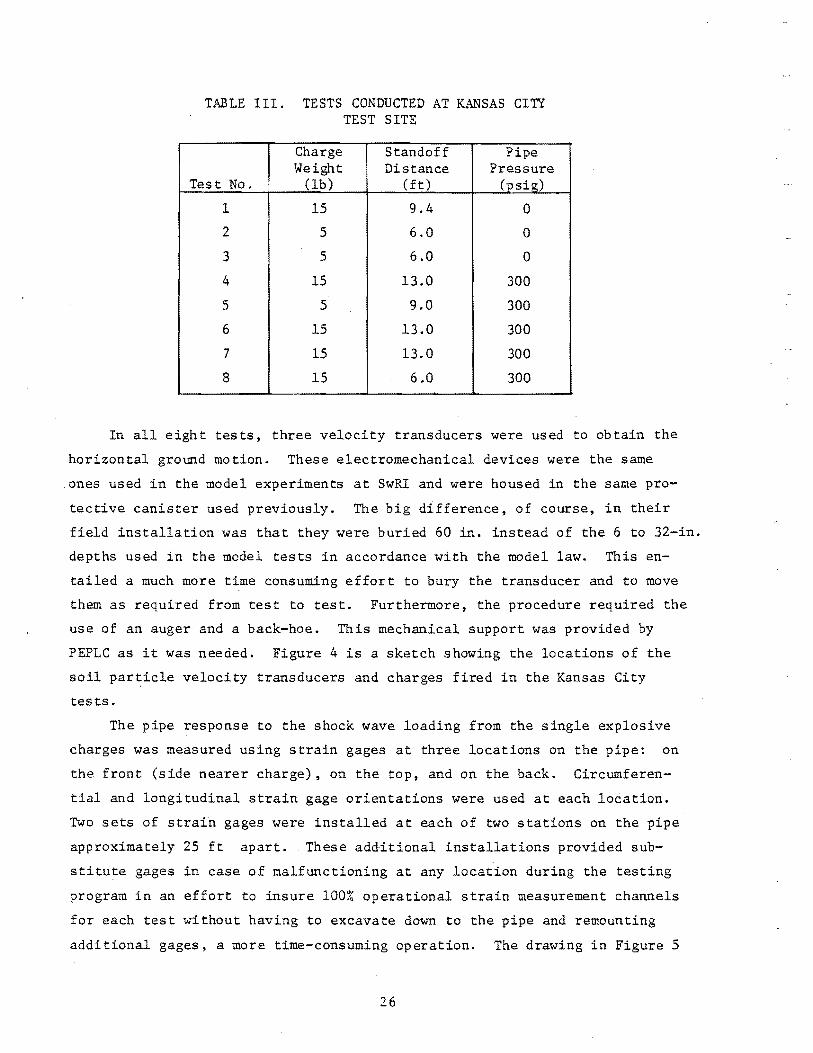
TABLE III. TESTS CONDUCTED AT KANSAS CITY TEST SITE

Charge Standoff Pipe Weight Distance Pressure

Test No. (lb) (ft) (psig)

1 15 9.4 0

2 5 6.0 0

3 5 6.0 0

4 15 13.0 300

5 5 9.0 300

6 15 13.0 300

7 15 13.0 300

8 15 6.0 300

In all eight tests, three velocity transducers were used to obtain the

horizontal ground motion. These electromechanical devices were the same

.ones used in the model experiments at SwRI and were housed in the same pro­

tective canister used previously. The big difference, of course, in their

field installation was that they were buried 60 in. instead of the 6 to 32-in.

depths used in the model tests in accordance with the model law. This en­

tailed a much more time consuming effort to bury the transducer and to move

them as required from test to test. Furthermore, the procedure required the

use of an auger and a back-hoe. This mechanical support was provided by

PEPLC as it was needed. Figure 4 is a sketch showing the locations of the

soil particle velocity transducers and charges fired in the Kansas City

tests.

The pipe response to the shock wave loading from the single explosive

charges was measured using strain gages at three locations on the pipe: on

the front (side nearer charge), on the top, and on the back. Circumferen­

tial and longitudinal strain gage orientations were used at each location.

Two sets of strain gages were installed at each of two stations on the pipe

approximately 25 ft apart. These additional installations provided sub­

stitute gages in case of malfunctioning at any location during the testing

program in an effort to insure 100% operational strain measurement channels

for each test without having to excavate down to the pipe and remounting

additional gages, a more time-consuming operation. The drawing in Figure 5

26

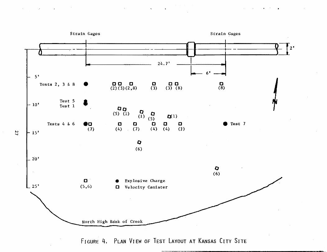
N ......

Strain Gages Strain Gages

-' 1 D - - -

24.7' T r- 5'

L 6'

Tests 2, 3 &. 8 • 00 0 0 00 0 {2) {3)(2 ,8) (3) {3) (8) {8)

Test 5 • 1- 10' Test 1 oo -

{ ..... , 0 Velocity Canister

North High Bank of Creek

FIGURE 4. PLAN VIEW OF TEST LAYOUT AT KANSAS CITY SITE

(} } EJ2'

, ~ ,,

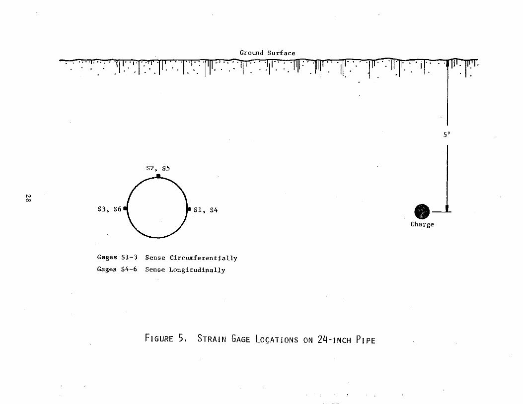
N CD

S2, SS

S3. S6 Sl. S4

Gages Sl-3 Sense Circumferentially

Gages S4-6 Sense Longitudinally

Ground Surface

FIGURE 5. STRAIN GAGE LOCATIONS ON 24-INCH PIPE

. 1

5'

• Charge

' '

'.

details the locations of one set of strain gages. All other sets of gages

were installed at similar points around the pipe.

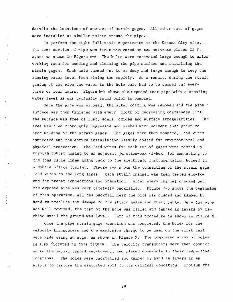
To perform the eight full-scale experiments a.t the Kansas City site,

the test section of pipe was first uncovered at two separate places 25 ft

apart as shown in Figure 6-a. The· holes were excavated large enough to allow

working room for sanding and cleaning the pipe surface and installing the

strain gages. Each hole turned out to be deep and large enough to keep the

seep~ng water level from rising too rapidly. As a result, during the strain

gaging of the pipe the water in the hole only had to be pumped out every

three or four hours. Figure 6-b shows the exposed test pipe with a standing

water level as was typically found prior to pumping.

Once the pipe was exposed, the outer coating was removed and the pipe

surface was then finished with emery cloth of decreasing coarseness until

the surface was free of rust, scale~ oxides and surface irregularities. The

area was then thoroughly degreased and washe.d with solvent just prior to

spot welding of the strain gages. The gages were then mounted, lead wires

connected and the entire installation heavily coated for environmental and

physical protection. The lead wires for each set of gages were routed up

through rubber hosing to an adjacent junction-box (J-box) for connecting to

the long cable lines going back to the electronic instrumentation housed in

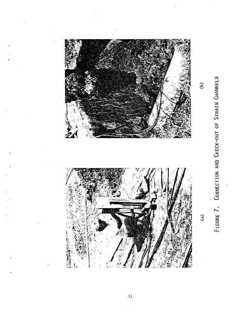
a mobile office trailer. Figure 7-a shows the connecting of the strain gage·

lead wires to the long lines. Each strain channel was then tested end-to­

end for proper connections and operation. After every channel checked out,

the exposed pipe was very carefully backfilled. Figure 7-b shows the beginning

of this operation. All the backfill near the pipe was placed and tamped by

hand to preclude any damage to the strain gages and their cable. Once the pipe

was well covered, the rest of the hole was filled and tamped in layers by ma­

chine until the ground was level. Part of this procedure is shown in Figure 8.

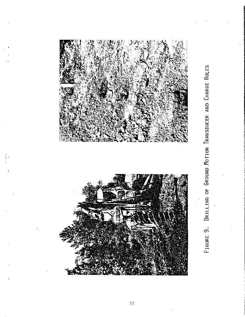
Once the pipe strain gage operation was completed, the holes for the

velocity transducers and the explosive charge to be used on the first test

were made using an auger as shown in Figure 9. The completed array of holes

is also pictured in this figure.. The velocity transducers were then connect­

ed to the J-box, tested end- to-end, and placed dmvn-ho le in their res pee ti ve

locations. The holes 111ere backfilled and tamped by hand in layers in an

effort to restore the disturbed soil to its original condition. Knowing the

29

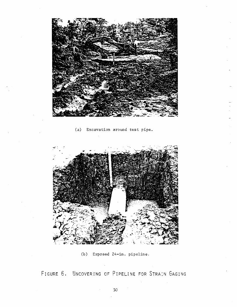
(a) Excavation around test pipe.

(b) Exposed 24-in. pipeline.

FIGURE 6. UNCOVERING OF PIPELINE FOR STRAIN GAGING

30

31

.-.. ..0 -

(/)

....I U.J z z <t: :I:

u z <t: 0:: 1-

C/.)

1.1. 0

1-=:l 0 I

::.I! u U.J

t3 0 z <t: z 0 -1-u U.J z z 0

u

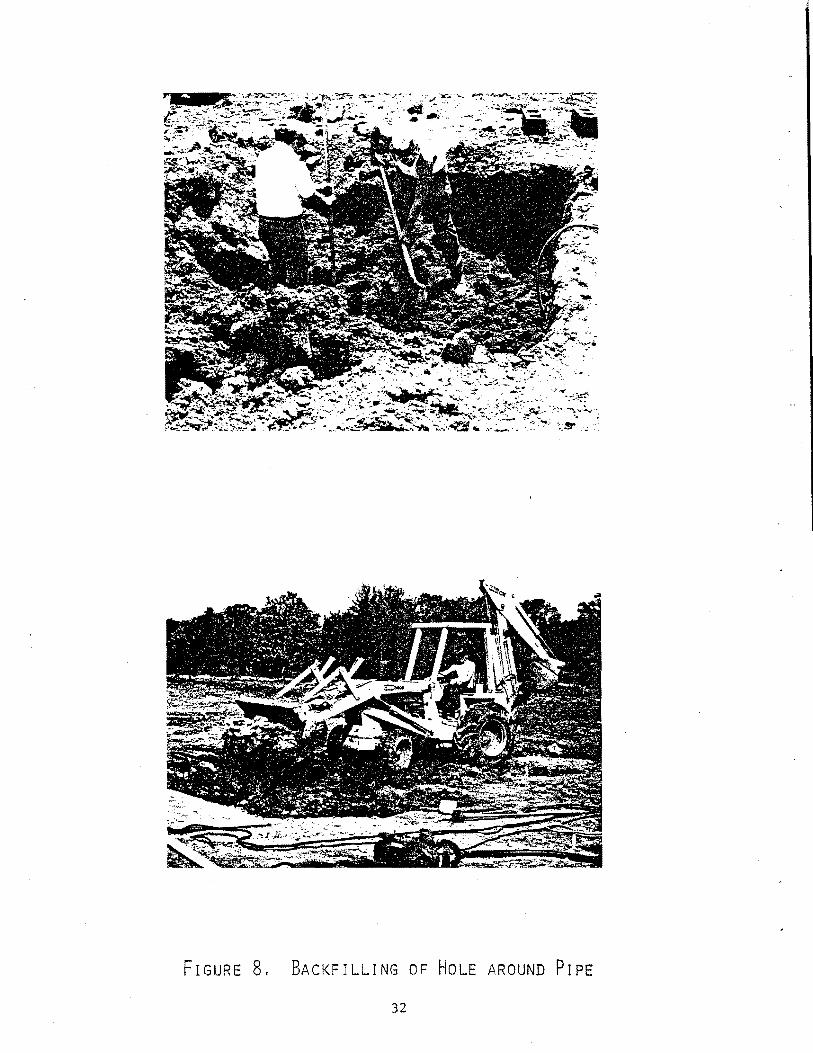
FIGURE 8. BACKFILLING OF HOLE AROUND PIPE

32

en LU .....J 0

:::I:

LU (.!)

a:: <:( :I:

u 0 z <:(

a:: LU u :::> 0 en z <:( a::

1-

z 0 -1- I 0

:E: I 0 z i => 1 0 t a:: I (...!:)

i u. I 0

(.!) I z I - l .....J .....J -a::

0

0'1

LU a:: => (.!) -LJ._

33

charge weight and its standoff from the pipe, the ground motions and pipe

strains expected were estimated using the results of the model experiments.

The gains and recording levels were then set for each measurement channel.

A countdown sequence and electrical calibration voltages were then recorded

for each measurement channel on the magnetic tape recorder. Once the com­

plete measurement system was ready for testing, the AN-FO explosive charge

was prepared by placing the cap, booster and the required amount of explosive

in a thin plastic container to protect it from any water or moisture. The

plastic bag was then sealed and placed down-hole as shown in Figure 10. At

the same time the site area was cleared of all personnel except for the

ordnance technician, and danger signs and audible flashers were placed at the

entrance road to the site to warn any unexpected visitors. Once the charge

hole was backfilled with tamped soil, the firing circuit was checked one last

time for continuity, and the power supply turned on for charging the firing

capacitor. The tape recorder was then started and the countdown sequence

played back. At time-zero, the charge was detonated. Figure 11 is a photo­

graph of one of the tests being fired using a 15-lb explosive charge. The

following two photographs, Figure 12, show the craters made by a 15-lb charge

and a 5-lb charge. After each test, the area around the crater was excavated

out about 2-ft past visible cracks in the soil and down 2 ft below the

location of the charge. The hole was then refilled in layers and tamped in

an effort to restore the ground back to its undisturbed condition. Velocity

transducers which required moving to a new location were dug.up and the hole

refilled and tamped. The velocity transducer and explosive hole layout for

the next experiment was then layed out and the holes redrilled. The same

procedures were followed for each subsequent test until all eight experiments

were completed.

Tests on Full-Scale Pipe-Kentucky

The last four experiments using a full-scale pipeline were conducted dur­

ing late fall of 1977, on an operational 30-in. diameter line near Madisonville,

Kentucky. The site was located on the TGTC right-of-way on the edge of a

cornfield and adjacent to a soybean field. Figure 13 shows two photographs

of the test site. The last mile to the site was accessible most of the time

only by foot or tracked vehicles because of the snow and rain making the soft

34

,• ~i I I.

I' .,

35

IJJ (!) a:: < :I:

u IJJ > (J)

0 _J 0... X

LJ.J

u.. 0

1-:z: IJJ :E: IJJ u < _J

0...

Cl :z: < :z: 0 -1-< a:: < 0... IJJ a::

0...

IJJ a:: :::J (!) -

FIGURE 11. DETONATION OF BURIED 15-LB, EXPLOSIVE CHARGE

36

UJ (,!) 0::: <( :::c u

IXl (j) ...J z

0 Ltl -1-......... <(

IXl z - 0 1-UJ

Cl

Q UJ

0::: ::::>

Q:l

>-IXl

UJ Q <(

::E: (j) 0::: UJ 1-<( 0:::

w

UJ N (,!) r-i 0::: <( UJ :::c 0::: u ::::>

(,!) -!XI LJ_ ...J

Ltl r-i

......... <( -

37

(a) View looking northwest from corn field.

(b) View looking east toward entrance to site.

FIGURE 13. KENTUCKY TEST SITE

38

ground extremely muddy. The pipe at the test site is buried approximately

5.5 ft to its centerline and its thickness is(cr:54~~The excavation

around the test pipe indicated a very uniform l~o~soft, reddish clay

down to at least 7.5 ft in depth. Although four tests were fired, five were

actually setup. Test No. 5 resulted in a misfire in the booster used which

precluded detonation of the AN-FO explosive. A subsequent rain made condi­

tions in the field impossible for setting up the test again the following

day. An ensuing snowstorm and extremely cold weather forecast for the week,

plus the necessity of placing the 30-in. line back in service prompted TGTC

to cancel a try for a fifth test and declare the program complete. The test

plan for the Kentucky site as originally outlined called for five point source

experiments with the charge (5 lb) buried to the same depth as the pipe on

three of them, and with the charge buried much deeper on the other two. How­

ever, the plan was slightly modified in the field. The charge weights used

were decreased on some tests so that a test at the closer standoff distance

could be conducted without loading the pipe past a maximum combined blast and

pressure stress set by TGTC. Also because of the extremely muddy conditions

and very soft soil in the test area, the holes for the explosive charges had

to be dug using a post hole digger. Consequently, a maximum charge depth of

only 7.5 ft could be obtained. Therefore, only one deeper charge test was

attempted. Unfortunately, it was to have been Test No. 5, which had the mis­

fire. Table IV lists the tests performed at the Kentucky test site.

TABLE IV. KENTUCKY TESTS

Charge Standoff Line Test Weight Distance Pressure No. (lb) (ft) (psig)

1 5 15 400

2 4 15 400

3 3 9 400

4 3 15 400

At least two ground motion transducers and six strain gages were record­

ed on each test in a similar way as was done in the Kansas City experiments.

Field support for uncovering the pipe, burying the transducers, and preparing

39

the ground after each test was provided by TGTC. The location of the velo­

city transducers and the explosive charges used in these tests are shown in

Figure 14. Circumferential and longitudinal strain gages were installed

at the locations shown in Figure 15. One set of gages, plus a back-up set!O

were installed as in the Kansas City tests: on the front, top and back of

the pipe. A second set of gages were mounted and rotated 45° from the first

to be used on the deeper charge tests.

To instrument this 30-in. pipe, a similar procedure was followed as in

the Kansas City tests. The pipe was first uncovered and an area of pipe

cleaned down to the bare metal for mounting the strain gages. Water in the

hole was again a problem and it was pumped out several times during the day

while installation of gages took place. The gages were then coated and the

clean section of pipe recovered prior to back-filling. After all the strain

gage channels were connected and checked out with their electronics, the hole

was filled and tamped. The holes were then dug for installing the velocity

transducers and the first charge. These channels were also checked end-to­

end before back-filling. The record instrumentation was then set--up, cali­

brated and a countdown sequence recorded. The AN-FO charge, properly water­

proofed, was then buried and at time-zero it was detonated. Figure 16 shows

the 5-lb charge being fired. As in all the other full-scale tests, after

each test the area around the crater was excavated with a back-hoe, and the

hole back-filled and tamped before the charge hole for the following test

was dug. This same procedure was followed until the testing program was com­

pleted.

Ground Motion Transducers

The preliminary analysis for predicting pipe response to buried explosive

detonations indicated that maximum horizontal soil particle velocity and dis­

placement were required to determine the forcing function. To measure these

two parameters, motion transducers were required to be placed at the locations

of interests in both the model and full-scale experiments. Because this pro­

gram was primarily designed for conducting tests using available technology

for making the required measurements, no efforts were undertaken to develop

new measurement methods or hardware. Existing transducers and techniques were

modified for application in this program. Most commercially available motion

40

• Strain Gages

I 2.5' l I 0 Pipe Ci

{\ I }

f I ~

0\

~ L. c

~~6'j ~

"' }-c • Explosive Charge

c Velocity Canister ~

"'

* CJ

PLAN VIEW

Ground Surface

:I ji ·I

ELEVATION VIE'I-7

FIGURE 14. FIELD LAYOUT OF KENTUCKY TESTS

41

~ N

S2, S5

S3, S6 Sl, S4

Gages Sl-3 and Sll-13 are circumferential.

Gages S4-6 and Sl4-16 are longitudinal.

5.5 1

e Charge

FIGURE 15. STRAIN GAGE LOCATIONS ON 30-INCH PIPE

'• ... ; ...

FIGURE 16. DETONATION OF BURIED 5-LB. ExPLOSIVE CHARGE

43

transducers are not designed for an environment of high-pressure or external

stress exerted on the transducer housing, as in the case of a high-explosive

generated stress wave in soil. Therefore, the transducers were installed in

a protective canister which also simplified placement procedure in the field

and provided weatherproofing. From data in the literature, a range of magni­

tudes and rise times of particle velocity and displacement that could be ex­

pected in these tests were obtained. Bell and Howell Type 4-155 piezoelectric

velocity transducers were chosen as the primary sensor for making the soil

velocity measurements. Peak displacement measurements were obtained by in­

tegrating the velocity trace using a manual digitizer and plotter with a

Hewlett-Packard Model 9830 microcomputer. The Type 4-155 transducer is a

small, rugged vibration transducer with .a high natural frequency which allows

a linear response over a wide frequency range. The high sensitivity makes it

desirable for low level velocity measurements which can be externally inte­

grated to provide displacement signals. Each unit combines within its housing

a piezoelectric accelerometer, an electrical impedance which allows the use

of long interconnecting cables between the sensor and the recording instru­

mentation. The usable velocity range of this type of sensor is 0.2 to 100

ips, with a dynamic frequency response of 1 to 2000Hz. The velocity trans­

ducer can withstand a shock acceleration of 100 g's peak without damage and

is sealed water tight. Figure 17 shows how this velocity sensor was connected

in all the tests performed to a power supply and a magnetic tape recorder

used to record the data. By recording the data at 15 or 30 ips and playing

it back at 1-7/8 ips, a time amplification factor of 16 allowed good time

resolution for recording the playback data on oscillograph recorder.

Since some of the scale model experiments required detonations very close

to the pipes and measurement of ground motions were wanted at comparable dis­

tances, a second type of sensor was also used in these experiments. These

transducers were piezoelectric accelerometers, PCB Model 302M46, with a full­

scale range of 2500 g's and a frequency response of 0.05 to 10,000 Hz. Since

the velocity transducers previously described can withstand only 100 g's of

shock acceleration, the accelerometers were used to determine how close to

the explosives ground motion measurements could be made without damaging the

velocity gage. The accelerometers were connected to the tape recorder as

shown in Figure 18. The canisters used to house the velocity gages were

44

J::­\..11

v T

,

....

.-II I

~·

..

Instrumentation Trailer

J-Box 1 J-Box 2

3-Conductor Cabl Power Supply

~ e - . - - - ,.. - + 30 v I I

I I I DC 't::_ ~ ''L., ~

.....

~ ..... .... Tape Recorder

Oscillogra ph

I Recorder I

tt-t -., + 1'-

FIGURE 17. CIRCUIT DIAGRAM FOR VELOCITY TRANSDUCER

.j::--0"

Accelerometer

J-Box 1 J-Box 2

I I

Instrumentation Trailer

Tape Recorder

Power Unit and Coupler

FIGURE 18. CIRCUIT DIAGRAM FOR AccELEROMETER

Oscillograph Recorder

designed so that an accelerometer could also be mounted at the same time.

The canisters were similar to some previously designed, tested, and used by

the U. S. Army Waterways Experiment Station to make ground motion measure­

ments. A sketch showing how a velocity gage and an accelerometer were

mounted in a canister is shown in Figure 19. A hose and fitting were used

to route the interconnecting cable from the canister to a junction-box above

ground. The hose provided physical and environmental protection to the cable.

The accelerometer data were also played back onto oscillograph paper, then

digitized and integrated to obtain velocity data to compare to that of the

velocity transducer. In some tests, an accelerometer was used by itself close­

in to the explosive charge. In these cases a similar, though smaller, canis­

ter was used since no velocity transducer was included. Because most of the

acceleration measurements and their integrated velocities were made to deter­

mine whether the velocity gage could be used at a given close-in standoff

distance, the data were not used in checking the analysis. Instead, the

direct velocity measurements, which are more accurate, and ~heir integrated

displacements were used. In the case of the displacements, which turned out

to be the controlling parameter in the analysis for most detonations near gas

lines, a double integration would have been required on the acceleration data,

thus increasing errors and inaccuracies. Consequently, no double integra­

tions were attempted.

The placement of the motion transducers in the field experiments re­

quired the digging of holes of the proper depth and slightly larger than the

canister used. Each velocity transducer and accelerometer was first inspect­

ed when received from the manufacturer by checking the factory calibration

over a frequency range of 20to 400Hz using a shake table at SwRI. Then it

was placed in a canister and the whole assembly mounted on the shake table

again to insure that the s~nsitivity remained constant. Then it was taken

to the field for placement. On the full-scale experiments the holes made

were up to 6 ft in depth. Figure 20 shows a typical canister placement down­

hole for the full-scale experiments.

Strain Gages

To measure the response of the pipes tested, strain gages were used at

various locations on the surface of each pipe. Two primary techniques for

47

PCB Accelerometer

Section A-A

Bell & Howell Velocity Transducer

1/32 Neoprene Gasket

1/4-20 UNC 1-in.-long Flathead Screws

Scale: 1/2" == 1'

FIGURE 19. GRoUND MoTION CANISTER AssEMBLY

48

I

. . l

I

! •

FIGURE 20. PLACEMENT OF VELOCITY CANISTER DowN-HOLE

mounting strain gages on specimens are available to the user: adhesive bond­

ing and spot welding. For most applications adhesive bonding of strain gages

is the common technique used, particularly if the size of the structure is

such that it can be taken inside during the installation. On the three pipes

used in the model scale experiments the Micro-Measurements Type CEA-06-125UT-

350. two element. 90° strain gage rosettes were bonded with M-BOND ··AE-10 epoxy

adhesive. Because all the gages were mounted along a longitudinal or circum­

fe~ential sensing direction, an orthogonal rosette was chosen to decrease in­

stallation time. Each rosette was connected to a four-conductor shielded cable,

with one pair of conductors attached to each gage element. After the rosette in­

stallation was complete it was protected against the environment using M-COAT F

coating. Figure 21 shows the 6-in. pipe with one set of strain gages in­

stalled and wired. and with the protective coating in pla.ce. After all the

gages were tested for proper operation, the instrumented pipes were placed

in the ground as shown in Figure 22 for the 3- and 6-in. pipes. In a similar

fashion. the last of the model pipes was instrumente·d. Figure 23 shows the

49

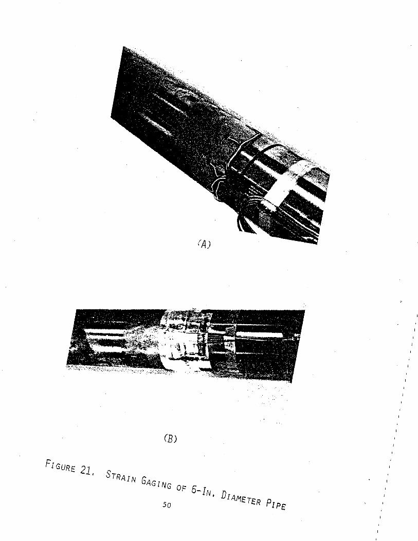
STRAIN GAGING OF 6-JN, DIAMETER PIP£ so

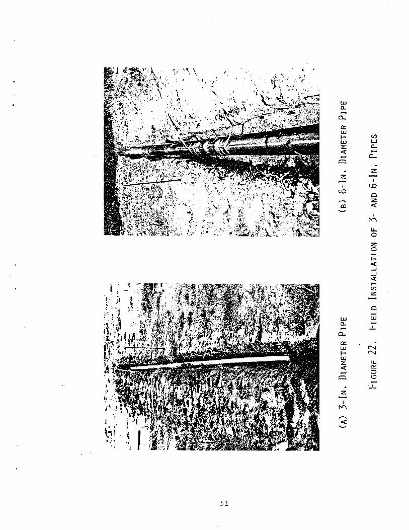
' ' , ' . l

"

51

LU a.. -0..

0::: LU en 1- LU LU a.. :E: .... <( 0.. -0

z -Z I - lD I lD Q

z - <( 1=0 .......,. I

LU a.. -0..

r-t'\

u.. 0

z 0 -1-<(

-' -' <( l­en z -Q -' LU -

0::: N LU N f-LU LU :E: 0::: <( ::::> ..... (.!)

0 ..... u_

z -I !'<\ -<( .......

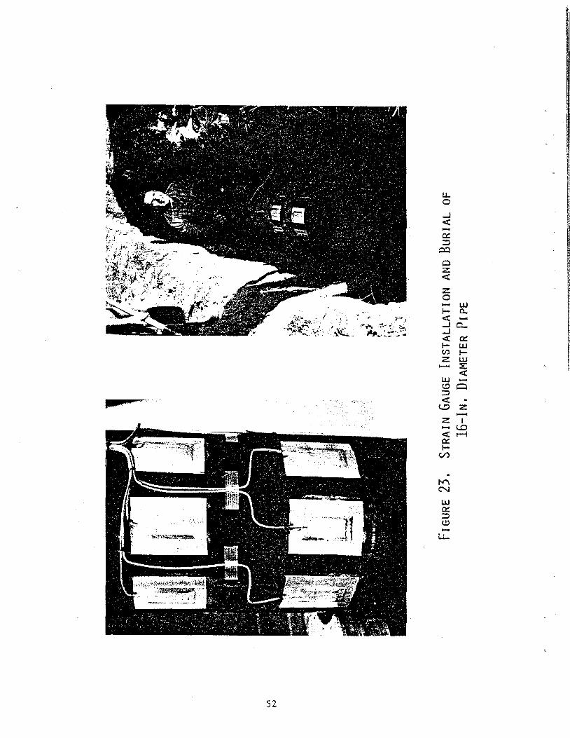
52

u... 0

...J <t ...... c::: :::::> ~

0 z <t

z 0 ...... 1-

~ ...J <t 1-CI)

z -

U.l 0..

a_

c::: U.l 1-U.I ::E: <t -0

z -z I - <..0 <t .....-i c::: 1-

(1')

-

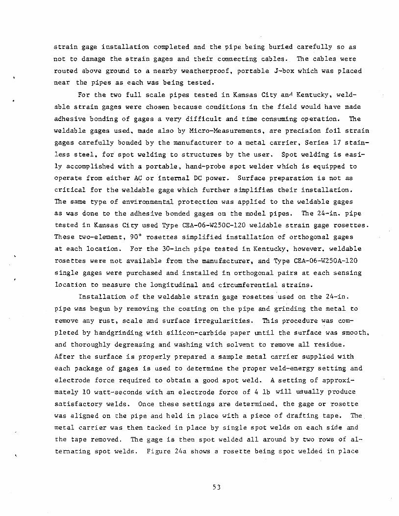
strain gage installation completed and the pipe being buried carefully so as

not to damage the strain gages and their connecting cables. The cables were

routed above ground to a nearby weatherproof, portable J-box which was placed

near the pipes as each was being tested.

For the two full scale pipes tested in Kansas City an~ Kentucky, weld­

able strain gages were chosen because conditions in the field would have made

adhesive bonding of gages a very difficult and time consuming operation. The

weldable gages used, made also by Micro-Measurements, are precision foil strain

gages carefully bonded by the manufacturer to a metal carrier, Series 17 stain­

less steel, for spot welding to structures by the user. Spot welding is easi­

ly accomplished with a portable, hand-probe spot welder which is equipped to

operate from either AC or internal DC power. Surface preparation is not as

critical for the weldable gage which further simplifies their installation.

The same type of environmental protection was applied to the weldable gages

as was done to the adhesive bonded gages on the model pipes. The 24-in. pipe

tested in Kansas City used Type CEA-06-W250C-120 weldable strain gage rosettes.

These two-element, 90° rosettes simplified installation of orthogonal gages

at each location. For the 30-inch pipe tested in Kentucky, however, weldable

rosettes were not available from the manufacturer, and Type CEA-06-W250A-120

single gages were purchased and installed in orthogonal pairs at each sensing

location to measure the longitudinal and circumferential strains.

Installation of the weldable strain gage rosettes used on the 24-in.

pipe was begun by removing the coating on the pipe and grinding the metal to

remove any rust, scale and surface irregularities. This procedure was com­

pleted by handgrinding with silicon-carbide paper until the surface was smooth,

and thoroughly degreasing and washing with solvent to remove all residue.

After the surface is properly prepared a sample metal carrier supplied with

each package of gages is used to determine the proper weld-energy setting and

electrode force required to obtain a good spot weld. A setting of approxi­

mately 10 watt-seconds with an electrode force of 4 lb will usually produce

satisfactory welds. Once these settings are determined, the gage or rosette

was aligned on the pipe and held in place with a piece of drafting tape. The

metal carrier was then tacked in place by single spot welds on each side and

the tape removed. The gage is then spot welded all around by two rows of al­

ternating spot welds. Figure 24a shows a rosette being spot welded in place

53

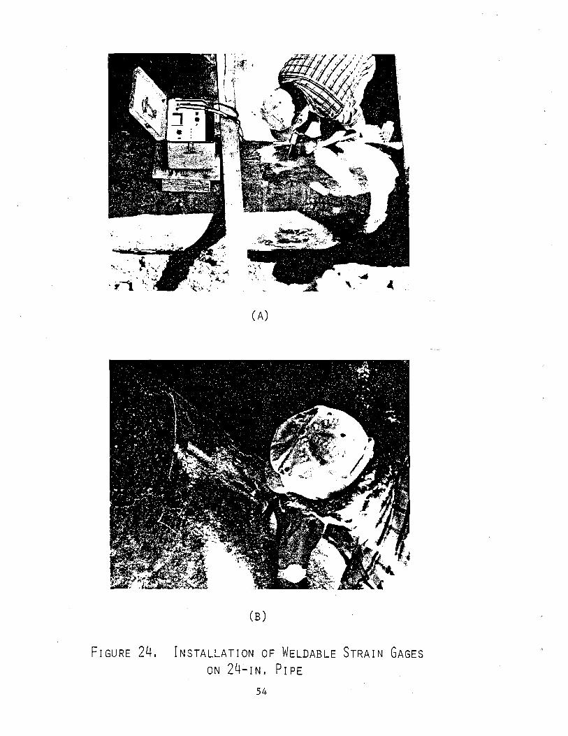
. ,, '1;,

(A)

(B)

FIGURE 24. INsTALLATioN oF vJELDABLE STRAIN GAGEs

ON 24-IN, PIPE

54

and the portable welder. Figure 24-b is a closer view of the welding opera­

tion. After the rosette was installed, cable leads were soldered to each

strain gage element and the element electrically checked before the complete

installation was covered with protective coating starting with a layer of

butyl-rubber, one of the components of theM-COAT F. This operation is

shown in Figure 24-c. For mechanical protection a patch of neoprene rubber

is placed over the butyl-rubber before aluminum tape is used as the final

cover. A liquid sealant is then used around all the edges of the aluminum

tape. Figure 24-d shows two complete installations of a pair of rosettes.

This figure also shows the lead wires completely sealed and placed into a

rubber hose for additional protection. This hose routed the cables to a

near-by J-box.

For the individual weldable gages used on the 30-in. pipe in Kentucky,

the installation of the gages was about the same as the rosettes in Kansas

City. However, because individual gages were used alignment at each loca­

tion prior to spot welding took more time. And, the one installation re­

quired down 45° from horizontal was more difficult to do than the rest.

Figure 25-a shows the spot welding of the gages at this location. The attach­

ment of cables and environmental protection, as shown on Figure 25b was

essentially the same.

Regardless of whether bondable or weldable gages were being used, each

element of the strain rosettes or individual gage was connected as a single

active arm of a Wheatstone bridge, using a three-wire hook-up and remote

electrical calibration connections. B&F Model 1-700 SG signal conditioner

units provided bridge completion and balance, excitation voltage to the

bridge, and a two-point electrical calibration. The output of each bridge

was amplified with a B&F Model 702A-10D differential, wide-band amplifier

and recorded on the same tape recorder used for the ground motion measure­

ments. Figure 26 shows the circuit diagram for the strain gages.

Record and Playback System

For the majority of the experiments, six recording tracks of a tape re­

corder were allocated for strain measurements as shown on Figure 27. Two to

four tracks were used for velocity channels and in some of the scale model

experiments two accelerometer channels were recorded also. Two of the 14

56

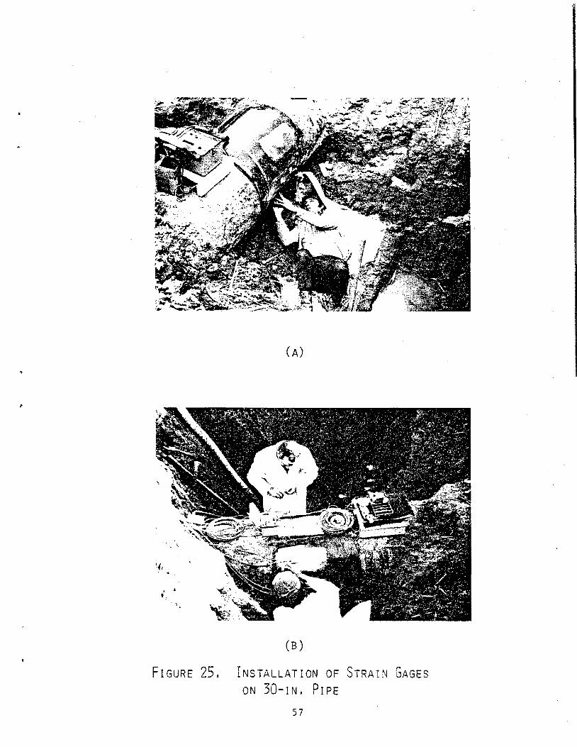
I'

(A)

(B)

FIGURE 25. INSTALLATION OF STRAIN GAGES

ON 30-IN. PIPE

57

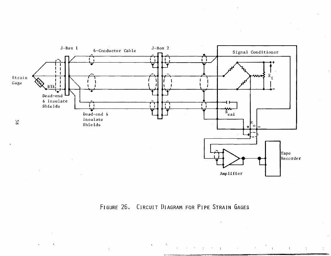
J-Box 1 J-Box 2 6-Conductor Cable • Signal Conditioner

t+

~!;:'" ~ _: : l f\: ( \ :"~lj( j ( ) I . /I""] Et

& Insulate 1 ~ - 1 1 .- 1 Shields ~

Dead-end & ~ J-.1 T I Real \J1 Insulate ()J Shields

Amplifier

fiGURE 26. CIRCUIT DIAGRAM FOR PIPE STRAIN GAGES

Tape Recorder

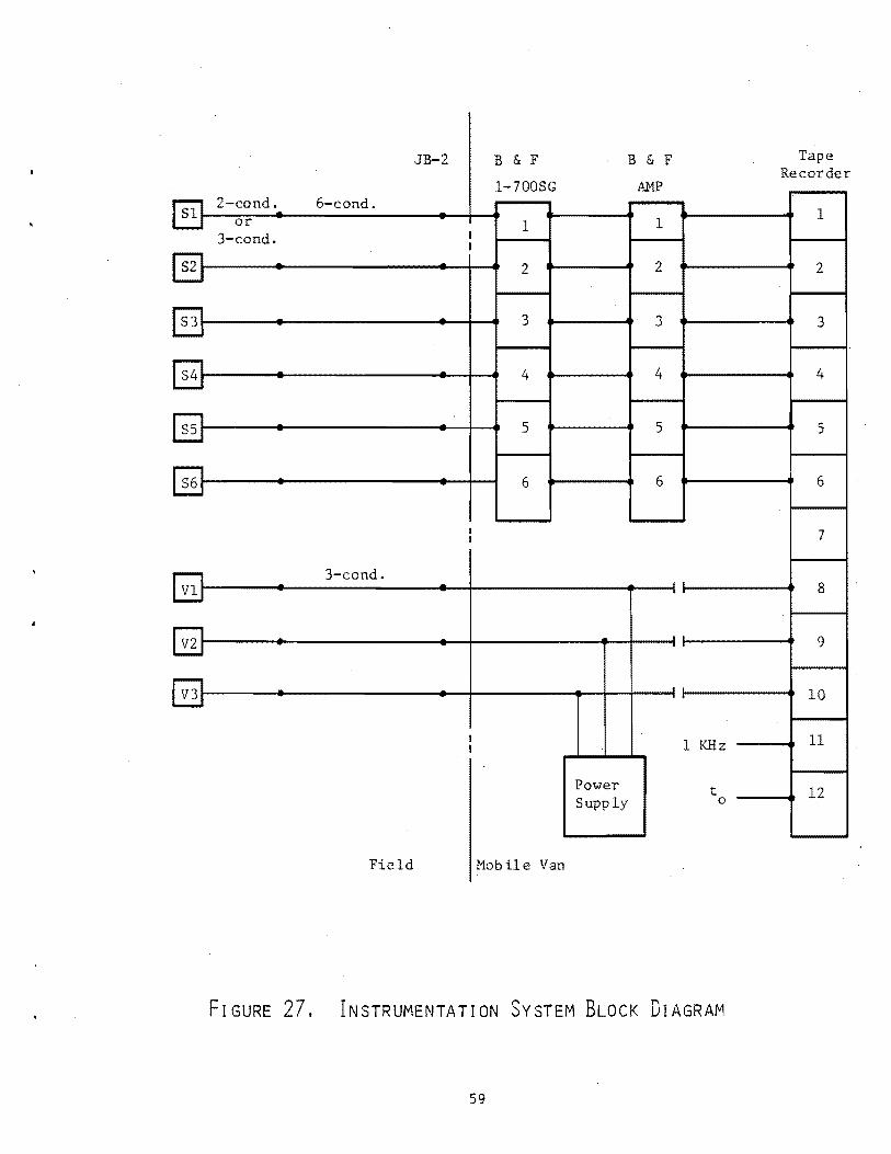
JB-2 B & F B & F Tape Recorder

l-700SG AMP

.. 2-cond. 6-cond.

Sl 1 or 1 1 3-cond. I

I

S2 2 2 2

S3 3 3 3

S4 4 4 4

ss 5 5 5

S6 6 6 6

I 7 I

3-cond. Vl

I 8

V2 l .. 9

V3 .

10 '

I 1 KHz 11 I

Power t 12 Supply 0

Field Hobile Van

FIGURE 27, INSTRUMENTATION SYSTEM BLOCK DIAGRAM

59

tracks available were reserved in all cases for recording time-zero and a

real-time reference signal. The data for the scale model experiments were

recorded on an Ampex FR-1900 tape recorder. The field data taken in the

Kansas City and Kentucky tests were recorded on a Honeywell Model 5600C sys­

tem. The recorded data were played back into a Bell & Howell Model 5-164

oscillograph system for quick-look data analysis and subsequent data reduc­

tion. The data were time extended on playback by factors of 16 or 32, and

using galvanometers having at least an 1,000 Hz upper frequency response

the data were not attenuated below a frequency of 16 kHz.

The oscillograph records were digitized at SwRI, manipulated, scaled

and plotted using a Hewlett-Packard Model 9830 microcomputer system. From

these plots, peak particle velocity, computed particle displacement and pipe

strain data were obtained for use in the analysis.

60

IV. EXPERIMENTAL RESULTS

The experimental data obtained from this program are presented in

this section. For each set of experiments conducte~ the horizontal ground

motion data and pipe strain data are presented separately. For most of

the 31 model-scale experiments,four velocity transducers, one accelero­

meter and six strain gage elements were recorded. Twenty of these experi­

ments used a single explosive charge as the source for loading the pipes.

On the remaining eleven model experiments, multiple charges representing

a line source were used. For the eight full-scale experiments done at

the Kansas City test site, single explosive charges were· used in all cases

to shock load the pipe tested with and without internal pressure. The

other four full-scale tests, which were conducted at the Kentucky test site,

used an operational pipeline with internal pressure, and single explosive

charges were detonated. Two to three velocity transducers and six strain

gages were recorded on the full-scale tests. In addition to the ground

motion and pipe strain measurements, other data such as average seismic

velocity in the soil, spot checks of soil water content, and small soil

sample densities were also measured throughout the testing programs. These

data will also be presented.

Ground Motions

To determine the forcing function which causes buried transmission

lines to be stressed due to nearby buried explosive detonations, maximum

horizontal soil particle velocity and displacement were measured in all

field experiments conducted in this program. In most of the 31 model tests

conducted, four velocity transducers and one accelerometer (mounted or1 the

same canister as the closer-in velocity sensor) were used to obtain the

ground motion data. In some cases a second accelerometer was also used

in a separate canister. Figure 1 (section III) shows the location of

these transducers in both the single and multicharge tests. Note that three

different transducer lines were used to minimize interference as the shock

waves propagated through the ground. Although the spacing varied between

canisters for different test conditions, the first canister was usually

61

buried at the same distance from the charge (or charge line) as the pipe

being tested.

The type and size of explosive used, and ground motion data obtained

in the 31 model experiments are summarized in Table V. This table lists

each test by number, the total charge weight used, whether the charge was

a point or a line source, and if a line source, the length of the line.

The line sources were composed of seven equal weight charges spaced equi­

distant, the center charge aligned with the center of the pipe, and the

charge line parallel to the pipe. Each charge was buried below the surface

the same distance as the center of the pipe in a given test. This distance

from the surface of the ground to the center of each charge is also listed

in the table. All the ground motion data are radial horizontal measure­

ments for the point sources and horizontal measurements along lines perpen­

dicular to the line sources. The headings in the table used to identify

each measurement correspond to those shown in Figure 1. For example, R1

is

the distance between the charge and the first ground motion canister contain­

ing a velocity transducer, u1 , and sometimes also an accelerometer, A1

•

The displacement ~l was obtained by integrating the velocity-time trace

of u1

. The velocity UAl was obtained by integrating the acceleration-time

trace of A1

• As previously mentioned, the data from A1 were primarily to

insure that the first velocity gage had not been exposed to a shock

environment that would have damaged and invalidated its data, and as a

check for the peak velocity measured. The second, third, and fourth (when

used) velocity sensors are listed in the table with their corresponding

distances from the charge and displacements obtained by integration. A

second accelerometer, A2

, was used in some tests primarily to monitor

close-in accelerations for determining whether the first velocity transducer

could be placed closer to the explosive source. Integrated velocities were

also obtained for these very close-in measurements and are reported here

for completeness, even though it was felt that they were not accurate enough

to be used in the analysis. In many cases these measurements were so close

to some of the line charges that the shock waves had not traveled a suffi­

cient distance to have formed a line source. Therefore, the data could not

have been used in the analysis anyway.

The last column lists the average seismic velocity obtained in each

test. This propagation velocity was obtained by determining the arrival time

62

TABLE V. SUMMARY OF HORIZONTAL GROUND MOTION DATA FROM MODEL TESTS

Ueptb Average • Charge Type Line of R U X A1 U R U X 8. U X R U X R A2 U Scismir

Test llelght of Length llurial 1 1 Ul 2

A1 2 2 U2 l 3 Ul 4 4 ··u4 A2 2

A2 V"1ocity No. _ill.L Source ~L ~:l .!!!J. ~ .i.!!!d_ .!!_eD ~ .li!l. ~ l!.!!..:l 1f.!:l ..lil>.ll .. li!!.:l 1f.!:l i!..e& J!!l!l 1f.!:l .{ie!Q_ i!..e& _j..!I>_I!.L ....

1 0.05 point -- 6 3.0 -- 4,437 9.5 -- -- -- -- -- -- -- -- -- -- -- --2 0.05 point -- 6 3.0 12.4 0.042 6,491 9.2 4.5 1.0 0.012 6.0 2.26 0.013 -- -- -- -- -- -- 958 3 0.05 point 6 3.0 -- -- -- -- -- -- -- -- -- -- -- -- -- --4 1.00 point 6 7.0 23.0 0.234 8,000 18.3 U.O 5.8 0.056 15.0 2.47 0.030 -- -- -- -- -- -- 922 5 0.40 point -- 12 4.0 13.0 0.105 5,900 10.0 8.0 5.8 0.050 12.0 2.1 0.016 -- -- -- -- -- -- 929 6 0.40 point -- 12 4.0 24.2 0.150 14,200 27.0 8.0 8.9 0.066 12.0 3.0 0.022 -- -- -- -- 895 7 1.00 point -- 12 7.0 15.4 0.160 -- -- 11.0 10.3 0.118 15.0 2.7 0.038 -- -- -- 3.0 31,230 54 1038 8 0.03 point -- 12 2.0 10.9 0.053 -- -- 4.0 2.3 0.018 6.0 0.8 0.005 -- -- -- 1.0 34,000 48 958 9 0.03 point -- 12 2.0 7.4 0.031 -- -- 4.0 1.7 0.011 6.0 0.92 0.006 -- -- -- 1.0 46,000 45 751

10 0.01 point -- 6 1.0 33.4 0.050 46,000 41.0 3.0 4.3 0.019 5.0 1.6 0.007 -- -- -- 0.5 290,000 90 1014 II 0.35 line 10.5 12 2.0 19.2 0.195 15,500 22.0 2.0 18.9 0.130 4.0 13.0 0.110 6.0 6.4 0.073 1.0 63,500 48 1110 !2 2.80 Uut> 14.4 12 5.0 25.9 0.41 -- -- 8.0 12.3 0.195 11.0 11.5 0.16 14.0 5.8 0.094 -- -- -- 738 13 2.80 lin" 9.0 12 5.0 36.3 1.35 -- -- 10.0 9.1 0.166 15.0 3.2 0.065 20.0 1.6 0.025 -- -- -- 679 14 2.80 llne 9.0 12 5.0 39.6 1.46 -- -- 10.0 9.1 0.136 15.0 2.2 0.044 20.0 1.6 0.023 3.0 24,400 72 780

0'\ 15 0.35 line 4.5 6 2.5 50.1 0.48 14,850 57.0 5.0 14.1 0.200 7.5 5.8 0.082 10.0 1.5 0.023 1.5 57,100 90 945 W 16 0.15 line 4.5 6 2.5 72.8 0.55 -- -- 5.0 17.2 0.240 7.5 7.9 0.108 10.0 2.0 0.031 1.5 110,000 128 711

ll 0.21 line 9.0 6 3.0 21.'fJ 0:19 7,003 18.0 5.0 8.1 0.114 7.0 5.0 0.051 - 10.0 0.011 -- -- -- , 829} 18 2.80 line 5.4 6 5.0 5i.s 1.49 -- -- 10.0 6.8 O.ll 15.0 4.6 0.075 20.0 1.0 0.043 1.0 54,800 130 734 19 0.21 lin<.: 2.7 12 1.5 66.5 0.52 -- 3.0 19.8 0.27 6.0 6.1 0.12 9.0 1.8 0.035 1.0 140,000 150 564 20 0.03 point -- 32 1.5 14.0 0.029 10,300 13.0 3.0 4.7 O.Oll 4.0 2.13 0.005 5.0 1.3 0.003 1.0 32,100 27.5 U38 21 0.03 point -- 32 1.5 10.4 0.039 -- 3.0 3.0 O.Oll 4.5 1.49 0.005 6.0 0.82 0.003 1.0 15,050 33 964 22 0.03 )>oint -- 32 1.0 57.4 0.185 47,050 60.0 2.5 2.2 0.010 4.0 1.50 0.004 5.5 0.51 0.001 0.5 270,000 140 llOO 23 O.OJ I>Dlot 32 1.0 44.2 O.ll3 40,620 46.0 2.5 3.3 0.01) 4.0 1.4 0.0057 5.5 0.69 0.003 0.5 200,000 124 975 21• 0.06 !J<>int 32 1.5 57.7 0.19 16,200 69.0 3.0 5 • .5 0.030 4.5 3.1 0.0018 6.0 1.33 0,006 1.0 95,500 97 86b 2) 0.06 point -- 32 1.75 40.5 0.187 24,050 50.0 3.2 5.1 0.029 4.75 3.0 0.0187 6.2 1.1 0.007 1.0 140,000 123 675 26 0.'15 lin" 19.8 !i 5.0 4.5 0.0415 -- -- 8.0 2.53 0.021 11.0 2.0 0.014 14.0 1.8 O.Oll -- -- -- 701 n 0.35 lin<! 19.8 6 5.0 4.11 0.041 -- -- 8.0 3.0 0.0225 11.0 2.5 0.018 14.0 2.0 0.013 -- -- -- 645 28 0.05 !>oint -- 6 1.5 44.2 0.270 -- 3.0 9.0 0.085 4.5 3.9 0.040 6.0 2.0 0.021 1.0 120,000 UO 568 29 0.05 point -- 6' 1.5 46.0 0.230 65,700 56.0 3.0 12.2 0.110 4.5 5.) 0.056 6.0 2.9 0.028 1.0 102,000 91 612 30 0.40 point -- 12 3.0 60.0 0.670 19,100 49.0 6.0 8.6 0.179 12.0 1.0 0.011 18.0 0.7 0.009 · -- -- 592 11 0.40 point -- 12 3.0 52.0 0.480 -- -- 6.0 8.2 0.180 12.0 0.8 -- 18.0 0.75 2.0 150,000 128 447

* Su~ exvlal)acion in t~Xt.

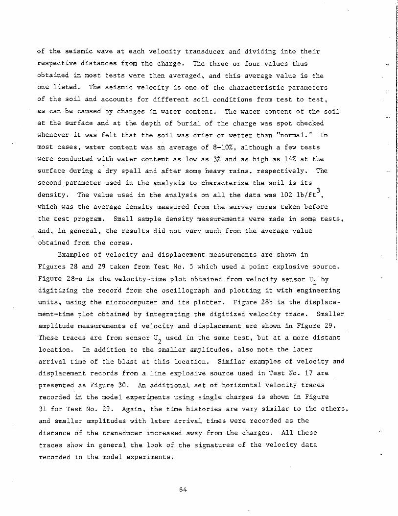
of the seismic wave at each velocity transducer and dividing into their

respective distances from the charge. The three or four values thus

obtained in most tests were then averaged, and this average value is the

one listed. The seismic velocity is one of the characteristic parameters

of the soil and accounts for different soil conditions from test to test,

as can be caused by changes in water content. The water content of the soil

at the surface and at the depth of burial of the charge was spot checked

whenever it was felt that the soil was drier or wetter than "normal." In

most cases, water content was an average of 8-10%, although a few tests

were conducted with water content as low as 3% and as high as 14% at the

surface during a dry spell and after some heavy rains, respectively. The

second parameter used in the analysis to characterize the soil is its

density. The value used in the analysis on all the data was 102 lb/ft 3 ,

which was the average density measured from the survey cores taken before

the test program. Small sample density measurements were made in some tests,

and, in general, the results did not vary much from the average value

obtained from the cores.

Examples of velocity and displacement measurements are shown in

Figures 28 and 29 taken from Test No. 5 which used a point explosive source.

Figure 28-a is the velocity-time plot obtained from velocity sensor u1 by

digitizing the record from the oscillograph and plotting it with engineering

units, using the microcomputer and its plotter. Figure 28b is the displace­

ment-time plot obtained by integrating the digitized velocity trace. Smaller

amplitude measurements of velocity and displacement are shown in Figure 29.

These traces are from sensor u2

used in the same test, but at a more distant

location. In addition to the smaller amplitudes, also note the later

arrival time of the blast at this location. Similar examples of velocity and

displacement records from a line explosive source used in Test No. 17 are

presented as Figure 30. An additional set of horizontal velocity traces

recorded in the model experiments using single charges is shown in Figure

31 for Test No. 29. Again, the time histories are very similar to the others,

and smaller amplitudes with later arrival times were recorded as the

distance of the transducer increased away from the charges. All these

traces show in general the look of the signatures of the velocity data

recorded in the model experiments.

64

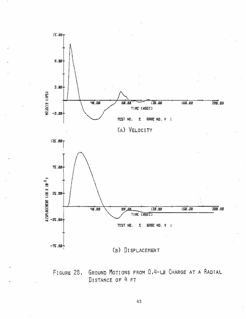
1;:.ea

!UlB

3 . .B.B ..... U"'

= .... >-..... c -l 1..1 -3 . .i!I.B >

7s:.BB

>c:

:;: 2S • .BB .... 8 ~ a: -l 1:1.. U"'

;;;; -2S.BB

-7s:.l1JB

!2B.BB TIHE: CHSEO

TEST NO. i 6R6t ND. V I

(A) VELOCITY

TEST NO. ~ 6Rst ND. V I

(B) DISPLACEMENT

20B.3B

FIGURE 28. GRoUND MoTIONS FROM 0.4-LB CHARGE AT A RADIAL DISTANCE OF 4 FT

65

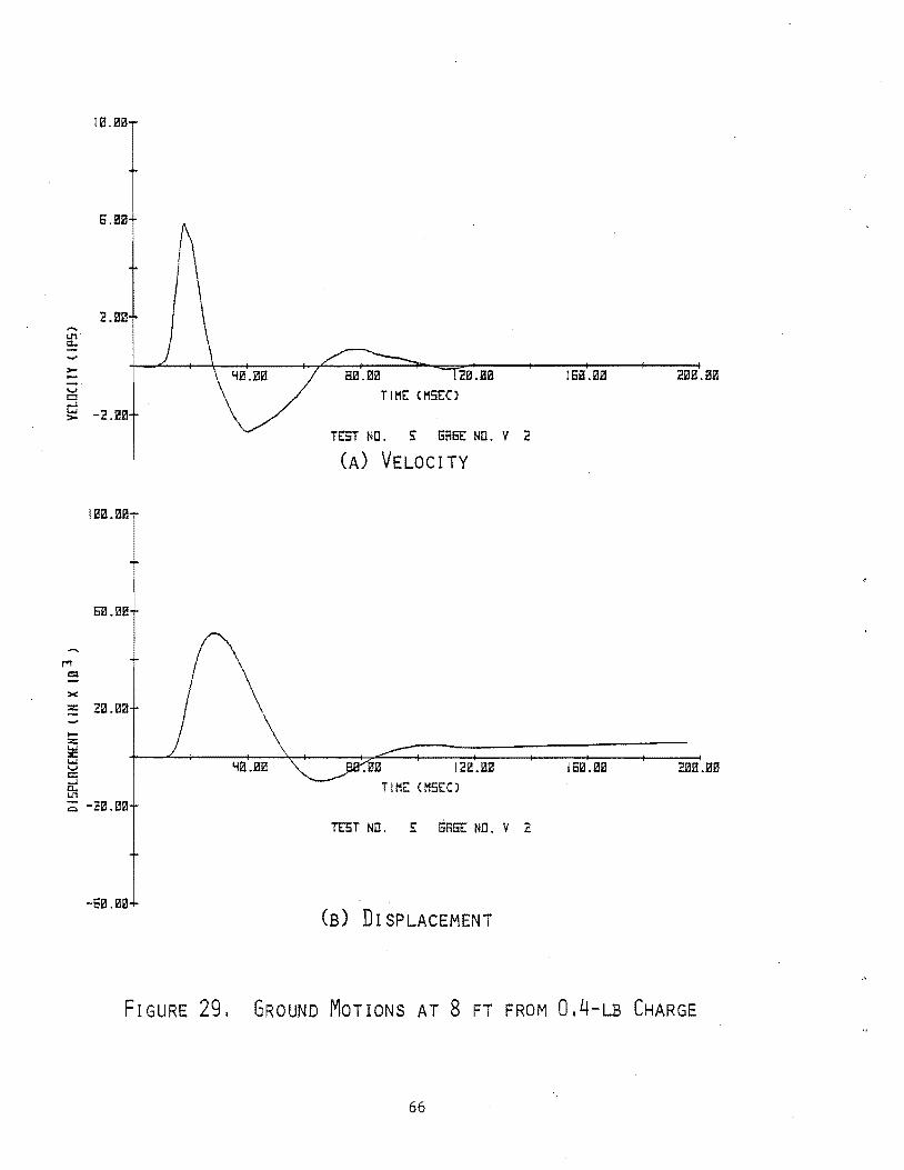
IB.Bl:'l

S.BB

2.Bii! ,..., Ln c.. -->-..... ._. t:l -l I..J -2JU:l >

IBB.l!U:l

Ei1U3B

z 21:3 .Bii!

...... :z: t....l z: L.W ._. c: -l c.. U"l

;;:::; -21um

-61LB0

!2EUIB

TIME <MSEO

TEST NO. s: GR6E ND. V

(A) VELOCITY

!21:U!IB

TIME CMSEO

2

TEST NO. S: GAEE NO. V 2

(B) DISPLACEMENT

tSB.lilB :i!BB .BPJ

ISIUIB :i!BfU!B

FIGURE 29. GROUND i~OTIONS AT 8FT FROM 0.4-LB CHARGE

66

VI1RX • 21.EB

IS.SB

S:.ml ... In !!:: oJ

>-.... ISUIB 2iliU1B .... s oo£.i2 1m ND. 17 liE Nil. V I

-IS.ml

(A) VELOCITY

lliB.i!B

1m NO. 17 !ifiEE Nil. V I

(B) DISPLACEMENT

FIGURE 30. GRoUND MoTIONS AT 3 FT FRoM 0.21-LB ExPLOSIVE LINE SouRcE

67

I<.SBI

1 7 .Slll

2.~ -"" ~ ..., >-1- sa.aa ~~~.aa l6~.BB v Q .--1

TIME Cl15EO w -2.5:3 >

TEST NO. 29 GnG'E: NO. V 2

(A) 3-FT LOCATION -7.::a

1um

~

2.ZZ I :J'l ::: ~

~ ,_ __.)2Z.Zfl a:!i!.lm ..... C7 TIME OiSEO --1 .... -?:.f!H, >

~ TE57 HD. a EREiE Nil. V J

I (B) 4.5-FT LOCATION ...t: ggl ~. T

FIGURE 31. HoRIZONTAL VELOCITIES FRoM 0.05-LB CHARGE

68

In the eight experiments conducted at the Kansas City test site.three

velocity transducers were used to obtain the horizontal ground motion data.

These transducers were placed in the ground at the same depth as the center

of the pipe, as was the case in all the model experiments. They were

located as shown in Figure 4 such that the first two transducers would

bracket the horizontal distance between the center of pipe and the

explosive. The third transducer used was then located further out to

obtain data over a reasonable range of distance. The peak soil velocities

and displacements obtained from the Kansas City experiments are shown in

Table VI by test number and distance of the velocity transducers from the

single charge sources used. For example in Test No. 4. which used a 15-lb

charge, the second canister containing velocity transducer u2 was located

a distance R2 of 12 ft away from the charge. The velocity-time trace

recorded by this channel is shown in Figure 32 along with its integration

to obtain the displacement. An example of the ground motions recorded from

a 5-lb charge is given in Figure 33.

Note that these data examples show particle velocities of the same

order of magnitude as those measured in the model experiments, an expected

result since the larger distances used for placing the transducers in the

full-scale tests were selected so that similar velocity amplitudes would

result. However, the velocity pulse durations would necessarily become

longer on the larger scale experiments. This was confirmed by the data.

Likewise, displacement amplitudes and durations were of larger magnitude

in the full-scale experiments.

The seismic wave propagation was also determined in the Kansas City

tests from the time of arrival of the wave at each canister location.

The average value for each test is also given in Table VI. Small soil

samples near the surface from the holes made for placing the charge and

velocity transducers on each test were checked for water content and density.

The water content was measured to be between 10-12% on all the Kansas City

tests and the density averaged close to 100 lb /ft3• m

The soil particle velocity and displacement data recorded in the four

full-scale tests conducted at the Kentucky test site were of similar nature

as those obtained in Kansas City. Table VII shows the peak values recorded.

The transducers were placed so as to obtain data at approximately the same

distance as that between the charge and the ~enter of the pipe. At leas.t

69

TABLE VI. RADIAL SOIL MOTION DATA FROM KANSAS CITY TESTS

Charge Rl ul ~1 R2 u2 XU2 R3 u3 XU3

Seismic Weight Velocity

Test No. (lb) (ft) (ips) (in) (ft) (ips) (in) (ft) (ips) (in) (fps)

1 15 7.0 55.4 0.92 10.0 14.3 0.28 15.0 3.6 0.057 900

2 5 5.0 159.7 2.62 8.0 80.0 2.18 -- -- -- 573

3 5 6.0 88.0 2.17 12.0 8.7 0.33 15.0 3.0 0.70 519

4 15 6.0 118.8 1.96 12.0 47.7 1.86 14.0 36.0 1. 21 1232

5 5 6.0 82.4 2.04 12.0 10.4 0.35 14.0 3.4 0.11 582

6 15 10.0 76.3 2.35 14.0 13.0 0.51 23.5 2.5 0.032 735

....... 7 15 8.0 98.6 5.5 16.0 8.2 0.25 24.0 3.6 0.11 792 0

8 15 8.0 138.0 4.78 16.0 6.2 0.34 24.0 1.24 0.049 622

Motion away from the charge is positive.

I .

TIME CHSE:O

-3!1!.~!1!

61:1.0111 121:1.01:1 18!1!.0111

TlHE C11SEO

TEST NO. 4 GAGE NO. V 2

FIGURE 32. RADIAL GROUND MOTIONS AT 12 FT FROM 15-LB CHARGE

71

Charge Rl ul Weight

Test No. (lb) (ft) (ips)

"1 5 6 --2 4 6 80.7

3 3 6 12.5

4 3 6 93.0

~ Motion away from charge is positive. ~

~

TABLE VII. GROUND MOTION DATA

XUl ~ u2 Xu2 R3 u3 ~3 Seismic Velocity

(in) (ft) (ips) (in) (ft) (ips) (in) (fps}

-- 12 22.0 0.29 1,230

1.51 12

0.79 12 14.1 0.33 18 2.1 0.036 974

1.57 12 18.8 0.25 1,480

2.~~ ....... Ll1 a.

>-t-

v r::::J -I w -2.~0 >

-7.~3

...... 1""'1

>< :z t0H.mil

t­:z w X:' w v c: -I a. U'1

;;;-rmum

-300.00

3£11:1.£11:1

TIME CHSEO

TEST NO. ~ EAGE NO. V 2

TlHE CHSEO

TEST NO. ~ GAGE NO. V 2

FIGURE 33. ~ADIAL SoiL MoTIONS AT 12 FT FRoM A 5-LB CHARGE

72

two measurements were attempted on each test as shown in Figure 14. However,

two data points were lost due to over-ranging the transducer in one case, and

severing of a cable splice in the second before data had been recorded.

Seismic velocity when obtainable is also shown in this table. Water content

in the soil measured near the surface ranged from 14-16% and soil density

averaged right at 101 lb /ft 3• Two examples of the soil motion data are m

shown as Figures 34 and 35. Both of these measurements were at the same

distance of a similar size charge as the ones in Figure 33 from the Kansas

City tests. However, the Kentucky data seems to have a higher peak velocity

with a much smaller duration. Because of the difference in seismic velocities

in these two sets of tests and because the data are plotted in dimensionless

form, the differences in amplitudes become small. This will be shown in a

later section of this report. Furthermore, the parameter that controls the

pipe response in the realm of interest is the soil displacement which, in its

dimensionless form,also plots well regardless of the test site.

Pipe Strains and Stresses

Strain measurements were made on both the model and full scale experi~

ments conducted in this program to quantitatively determine the response of

pipelines to nearby underground detonations. For use as the 3- and 6-inch

pipes, MT-1020 carbon steel tubing with a manufacturer specified minimum ul­

timate tensile strength of 65,000 psi was used. The specified minimum yield

strength (SMYS) was 55,000 psi. However, tensile tests performed on coupons

from these pipes at SwRI showed the ultimate tensile strength to be about

80,000 psi which would give an estimated yield strength of about 68,000 psi.

The 16-in. pipe used was ASTM A53, Grade B with a SMYS of 35,000 psi. Because

the principal modes of pipe response were not known, the 31 model experiments

used five different strain gage locations around the upper half-circumference

of each model pipe as shown in Figure 2. Two-element rosettes were used so

that both circumferential and logitudinal strain measurements would be possi­

ble at each location.

The testing program was begun by recording the five circumferential

strains since it was felt that these would be the larger·strains. Also,

the mode of the pipe response in this direction needed to be determined so

that those gages recording redundant or lower peak strains could be dropped

74

-~ -,.. 1-

~ -I 1.1 ;llo

-..., lSI

IS.ml

s.aa

~.as

-IS.iil

-:as:.aa

IB.ILBB

FIGURE 34. RADIAL

.213 TII'IE CMS£0

TEST NO. 6'flE NO. V 2

l8iUI111

Tl HE <115EO

TEET NO. EMEE: NO. V 2

(jA c;,\1 '/

!

SorL MoTIONS AT 12 FT FROM A 5-LB CHARGE 75

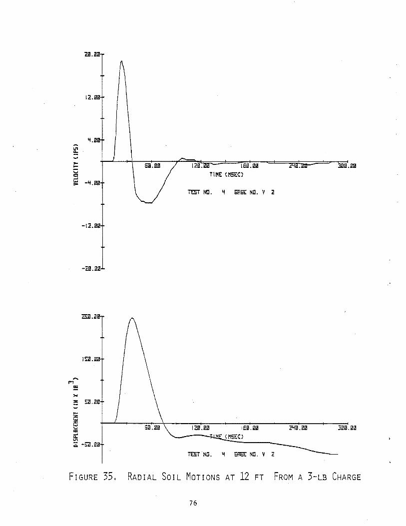
2B . .a

12.BB

-12.B9

-auua

I~.D

113iUli TIME (M5E<:)

TE:iT ND. "i SE!EiE ND. V 2

TEST ND • 1.1 EifE" ND . V 2

FIGURE 35. RADIAL SoiL MoTIONS AT 12 FT FROM A 3-LB CHARGE

76

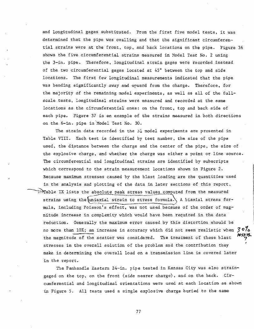
and longitudinal gages substituted. From the first five model tests, it was

determined that the pipe was ovalling and that the significant circumferen­

tial strains were at the front, top, and back locations on the pipe. Figure 36

shows the five circumferential strains measured in Model Test No. 2 using

the 3-in. pipe. Therefore, longitudinal strain gages were recorded instead

of the two circumferential gages located at 45° between the top and side

locations. The first few longitudinal measurements indicated that the pipe

was bending significantly away and upward from the charge. Therefore, for

the majority of the remaining model experiments, as well as all of the full­

scale tests, longitudinal strains were measured and recorded at the same

locations as the circumferential ones: on the front, top and back side of

each pipe. Figure 37 is an example of the strains measured in both directions

on the 6-in. pipe in Model Test No. 30.

The strain data recorded in the Jl model experiments are presented in

Table VIII. Each test is identified by test number, the size of the pipe

used, the distance between the charge and the center of the pipe, the size of

the explosive charge, and whether the charge was either a point or line source.

The circumferential and longitudinal strains are identified by subscripts

which correspond to the strain measurement locations shown in Figure 2.

Because maximum stresses caused by the blast loading are the quantities used

in the analysis and plotting of the data in later sections of this report,

~able IX lists the absolute peak ~~ss,_~~.~~tt~S9.!!J.PUted from the measured

strains using the~ial st~ to stress f~rmul~ A biaxial stress for­

mula, including Poisson's effect, was not used because of the order of mag­

nitude increase in complexity which would have been required in the data

reduction. Generally the maximum error caused by this distortion should be

no more than 10%; an increase in accuracy which did not seem realistic when J 0 'fo the magnitude of the scatter was considered. The treatment of these blast AO$~~ stresses in the overall solution of the problem and the contribution they

make in determining the overall load on a transmission line is covered later

in the report.

The Panhandle Eastern 24-in. pipe tested in Kansas City was also strain­

gaged on the top, on the front (side nearer charge), and on the back. Cir­

cumferential and longitudinal orientations were used at each location as shown

in Figure 5. All tests used a single explosive charge buried to the same

77

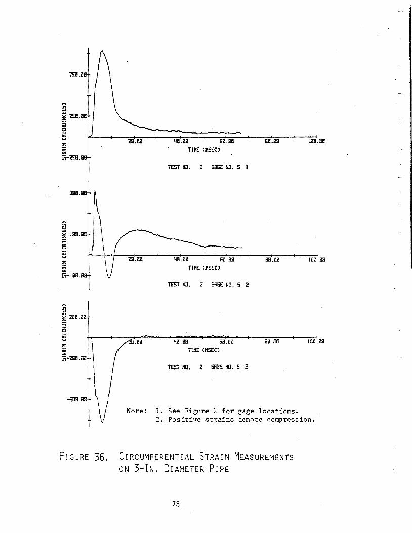
7SB.BS

-~ ~ 2SB.BB

e z: -:r.: a: g:

t:;;-2SB.BB

3i!IB.B

c:; f5 i:

= a: a:: tii-li!lil.9If

-U"l I..J

~ 2BB.BB Cl a:: .... :IC

= a: a: tii·2BB . .Bil

...ena.aa

aUB

.za

5B.BB BB.BB IBIU!B

TIKE CHSEO

TEST ND. 2 Ell'6'E NO. 5

~B.i!B SB.aa 8H.mJ I~B.lilB

TillE Cl15£()

TEST NO. 2 Eiil6E N!J. 5 2

~B.mJ 5iU!a BB • .IJB l.il.iLHB Tl11E 015£()

T£5T ND • 2 EflGE Ntl. 5 3

1. See Figure 2 for gage locations. 2. Positive strains denote compression.

FIGURE 36, CIRCUMFERENTIAL STRAIN MEASUREMENTS ON 3-IN. DIAMETER PIPE

78

12.H.BB

z: - 21'1.l!B SB.i!B SB • .BB IBB.mt

2 G:IEE: NO • 5 'i

-12B.ii!

Note: 1. See Figure 2 for gage locations. 2. Positive strains denote compression.

EiiUUUl

-~ 2BB.f.l3

5 z: - 21'1.118 liB JlS liB • .BB aa . .aa IBiU!B

Tl HE: ( 115£()

Tt5T Nil. 2 6FlEiE ND. 5 S:

-61!8 • .1!11

FIGURE 36, CIRCUMFERENTIAL STRAIN MEASUREMENTS ON 3-IN. DIAMETER PIPE CCoNT'o.)

79

smua

IUl.il TIM£ U!SE<:)

mrr liD. :m SHSE 11!1. s

2m! .mt ::miUifl Tl!!£ CI1SE()

n:sr liD. :m 6flt:i£ N.D • s J

Note: 1. See Figure 2 for gage locations. 2. Positive strains denote compression.

TIM£ (:15£0

n:sT ND. :ill 6i1EE N.D • 5 S:

(A) CIRCUMFERENTIAL STRAINS

FIGURE 37, STRAIN MEASUREMENTS FOR 6-!N. PIPE

80

-U1

liml.

~ 2m!. C't e r. ... ~

~ tii-2mt.

-~ ~ 1ruum C'l

e r. ....

-EUR

n:5T ND. JB EiiiEE Nil. 5 S b

2m1. ms :ma • .aa Lim! • .as TillE 015[ <:)

miT Nll. JB SREE !«1. 5 a ~

2m! • .as ::ma • .aa t.mi:UIB TillE(!&<:)

TE5T NO. :m 6RE£ Nil. 5 I.IJ t 0

(B) LONGITUDINAL STRAINS

FIGURE 37. STRAIN MEASUREMENTS FOR 6-IN. PIPE CCONT'D.)

81

sruum

srul.l!B

TABLE VIII. MAXIMUM STRAINS FROM MODEL EXPERIMENTS

Standoff Charge Type - Circumferential Strains Longitudinal Strains o.o.

Test Pipe Distance Weight of Sl S2 S3 S4 S5 S6 sa SlO No. (in) (ft) (lb) Source (l-!E) (IJd (llE) (lle;) (IJd (pt) ().IE:) (lld

1 2.95 1.5 0.05 pt. 474 -- -360 -175 253 2 2.95 1.5 0.05 pt. 1,039 311 -830 -158 612 3 2.95 1.5 0.05 pt. 844 443 -590 -- 875 4 2.95 11.0 1.00 pt. 80.7 74.9 -80 -37 112 5 5.95 3.0 0.40 pt. 466 171 -590 241 608 6 5.95 3.0 0.40 pt. 707 -90 -930 849 592 -520 7 5.95 11.0 1.00 pt. 90.6 -120 102 127 -44 -137 8 5.95 2.0 0.03 pt. 156 -135 106 169 -73 -117 9 5.95 1.0 0.03 pt. 996 -600 629 548 -2:18

10 2.95 0.75 0.03 pt. 1,075 -980 1,217 580 -215 868 11 5.95 5.0 0.35 line 140 .:.230 -- 239 -76 12 5. 95 8.0 2.8 line 302 -360 339 276 -190 -285

(X) 13 5;95 5.0 2.8 line 673 -850 942 724 -338 -825 N

14 5.95 5.0 2.8 line 424 -520 713 734 -435 -850 15 2.95 2.5 0.35 line 1,355 -1,025 1,084 600 -480 -535 16 2.95 2.5 0.35 line 1,395 -1,080 998 620 -570 -583 17 2.95 5.0 0.21 line 109 -67 115 140 -51 18 2.95 3.0 2.8 line 3,898 -2,640 2,308 1,550 -1,780 -1,396 19 5.95 1.5 0.21 line 1,14 7 -1,750 1,371 1,304 -255 -1,125 20 16.0 3.0 0.03 pt. 27 .It -15.0 19.4 16.7 -5.0 21 16.0 1.5 0.03 pt. 477 -240 238 205 -105 70 22 16.0 1.0 0.03 pt. 312 -168 155 158 -85 23 16.0 1.0 0.03 pt. -- -865 572 -- -270 246 24 16.0 1.5 0.06 pt. 214 -152 119 -85 25 16.0 1. 25 0.06 pt. 564 -330 298 -153 26 2.95 8.0 0.35 line 42 -27 37 48 46 -42.4 27 2.95 8.0 0.35 line 43 -29 42 54 -51 -61 28 2.95 1.5 0.05 p ':. 337 -200 192 490 -263 -410 29 2.95 1.5 0.05 pt. 463 -380 342 620 -260 -565 30 5. 95 3.0 0.40 pt. 564 -620 574 666 . -390 -620 31 5.95 3.0 0.40 pt. 473 -560 518 627 -410 -560

Positive strains denote compression.

~- _ ~'-- _L:o·:~-1-" j T''"!"?'??'ni!Cll·

TABLE IX. MAXIMUM BLAST PIPE STRESSES FOR MODEL TESTS

Standoff Charge Type Circumferential Longitudinal Test Pipe Distance Weight of Stress Stress No. (in) (ft) (lb) Source (psi) (psi)

1 2.95 1.5 0.05 pt. 14,200

2 2.95 1.5 0.05 pt. 31,200

3 2.95 1.5 0.05 pt. 26,300

4 2.95 11.0 1.00 pt. 3,400

5 5.95 3.0 0.40 pt. 18,200

6 5.95 3.0 0.40 pt. 27,900 17,800

7 5.95 '11.0 1.00 pt. 3,600 4,100

8 5.95 2.0 0.03 pt. 4,700 5,100

9 5.95 1.0 0.03 pt. 29,900 16,400

10 2.95 0.75 0.03 pt. 36,500 26,000

11 5.95 5.0 0.35 line 6,900 7,200

12' 5.95 8.0 2.8 line 10,800 8,600

13 5.95 5.0 2.8 line 28,300 24,800

14 5.95 5.0 2.8 line 21,400 25,500

15 2.95 2.5 0.35 line 40,700 18,000

16 2.95 2.5 0.35 line 41,900 18,600

17 2.95 5.0 0.21 line 3,500 ~ 4,200

18 2.95 3.0 2.8 line plastic yield 53,400

19 5.95 1.5 0.21 line 52,500 39,100

20 16.0 3.0 0.03 pt. 820 500

21 16.0 1.5 0.03 pt. 14,300 6,200

22 16.0 1.0 0.03 pt. 9,400 4,700

23 16.0 1.0 0.03 pt. 26,000 8,100

24 16.0 1.5 0.06 pt. 6,400 3,600

25 16.0 1.25 0.06 pt. 16,900 8,900

26 2.95 8.0 0.35 line 1,300 1,400

27 2.95 8.0 0.35 line 1,300 1,800

28 2.95 1.5 0.05 pt. 10,100 14' 700

29 2.95 1.5 0.05 pt. 13 '900 18,600

30 5.95 3.0 0.40 pt. 18,600 20,000

31 5.95 3.0 0.40 pt. 16,800 18,800

83

depth as the center of the pipe. This out-of-service length of pipe was

tested with no internal pressure on the first three tests, and with a pres­

sure of 300 psig for the last five tests. Typical strain data recorded

in the unpressurized full-scale experiments are shown in Figure 38 for ·

Test No. 3 in which three circumferential and three longitudinal measure­

ments were made. Note that the character of these time histories are very

similar to those from the model experiments shown earlier except that time

durations are longer.

For the pressurized tests, the recorded strains for each test were

also blast-induced because each strain channel was reset before each test.

Howeve.r, the strain gages had been recorded during the pressurization pro­

cess to determine the strain levels seen by each strain gage due to the

internal pressure only right after pressurization. The three circumferen­

tial channels recorded an average tensile strain of about 310~E and the

three longitudinal channels an average tensile strain of about 75~E.

Allowing for some restraint to the ~ipe by the soil around it, these strains

· agree well with the levels that would be expected from the 300 psig internal

pressure. Therefore, these strains can be superimposed on those resulting

from the blast loading to obtain a composite strain-time history. For

example, Figure 39 shows the strains recorded on Test No. 6 from the blast

only while Figure 40 shows the composite strains due to the blast and

internal pressure load.

The blast strain measurements made in the Kansas City full-scale

experiments are listed in Table X by test number. The size of the single

charge used and its distance to the pipe are also given. The circumferential

and longitudinal strains are identified by subscripts which are defined in

Figure 5. In a similar way, the combined peak strains from the blast loading

and the '!11t~~~J..~ pressure are presented in Table XI for

Test Nos. 4-8. The absolute value of the maximum stresses due to the blast

loading only computed from the measured peak strains are listed in Table XII.

These data points are also used in developing the solution for predicting

pipe response to buried detonations in later sections of this report.

Finally, the last set of strain measurements were made on a Texas Gas

Transmission Corporation 30-in. operational line with a specified minimum

yield strength of 52,000 psi located in Kentucky. This pipe was strain

gaged in a similar fashion as the Kansas City line. Circumferential and

84

""' Ll'l w

531!.013

~ 20t'U'!!il t::l cr::: v ::s::: .... :z r::c cr::: tii-21313 . liUJ

""' Ll'l

!:!:! ~ '2S:B.£JfJ Cl cr::: v ::s::: .... :z: a: a: tii-2S:IiU1121

5Biil.l:ll3

..... Ll'l

tx! ~ 2\?Ja.flfl

31ala.BI3

TIHE CHSEO

TEST NO. 3 GAGE NO. 5 I

10lil.kl0 S:B!il.Bii! --------TEST NO. 3 GAGE NO. 5 2

Note: 1. See Figure 5 for gage locations. 2. Positive strains denote compression.

t::l 0::

~ llr---~--~~----~----~----~----+-----+-----+-----+---~

t ... J !HI:U'l111 2liUl.H111 JBI:l.ml 'iflH.xm s:~m .lUl

TIHE: (HSEO

I TEST NO. 3 GAGE NO. s 3

(A) CIRCUMFERENTIAL

FIGURE 38. BLAST STRAIN RECORDS FOR 24-INCH PIPE 85

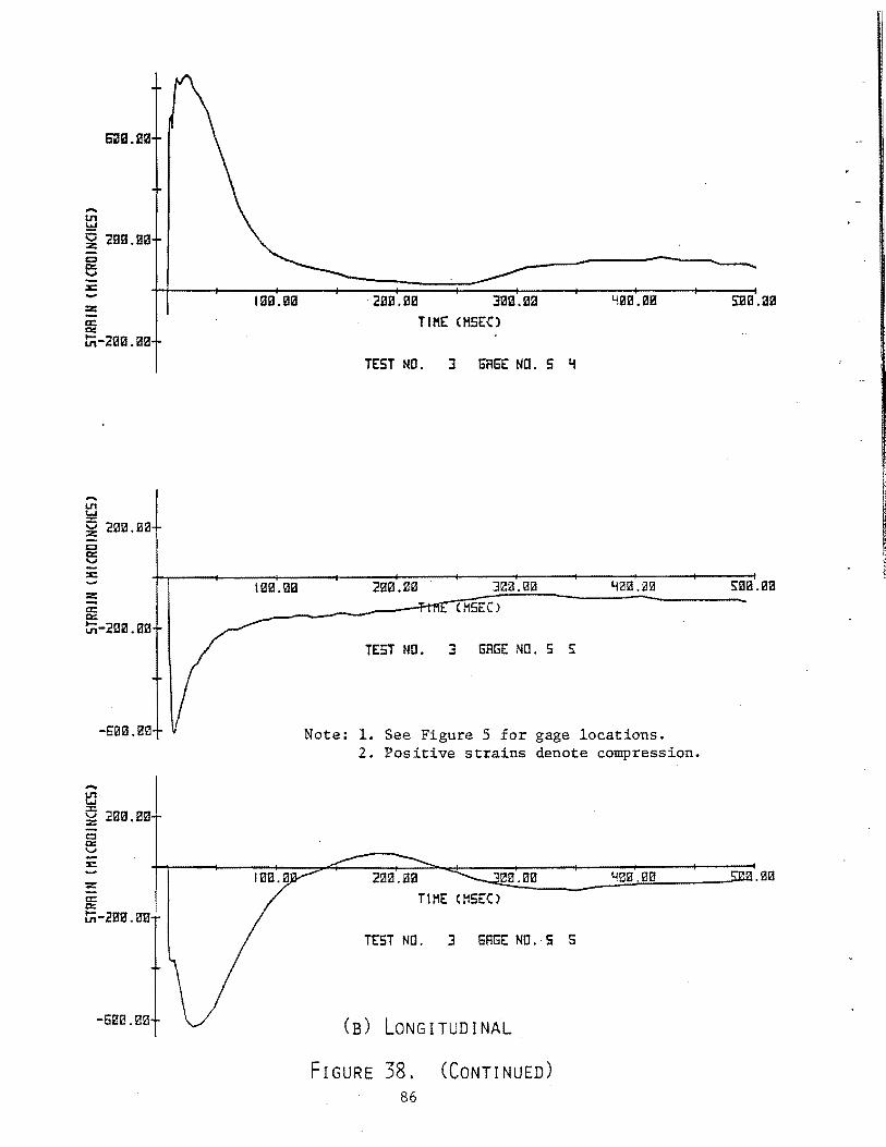
.... U'1 w ~ 21UUIB c 13 .::c ....

.... 1.11 w :c

. ?.iE 2mL a a c 13 .::c

z a: 0::.

l:ii-2Biil.Biil

.... U'1' w ::c ~ 21il3.B3 c::::l 0:: v :s::

:z: a: 0::

tn-23B .BB

IBB.BB 2BB.BB 30B.BB TIME CHSEO

TEST NO. 3 GAGE NO. 5 Y

TEST NO. 3 GAGE NO. 5 S

Note: 1. See Figure 5 for gage locations. 2. Positive strains denote compression •

TEST NO. 3 GAGE N0.-5 5

(B) LoNGITUDINAL

FIGURE 38. 86

(CONTINUED)

......

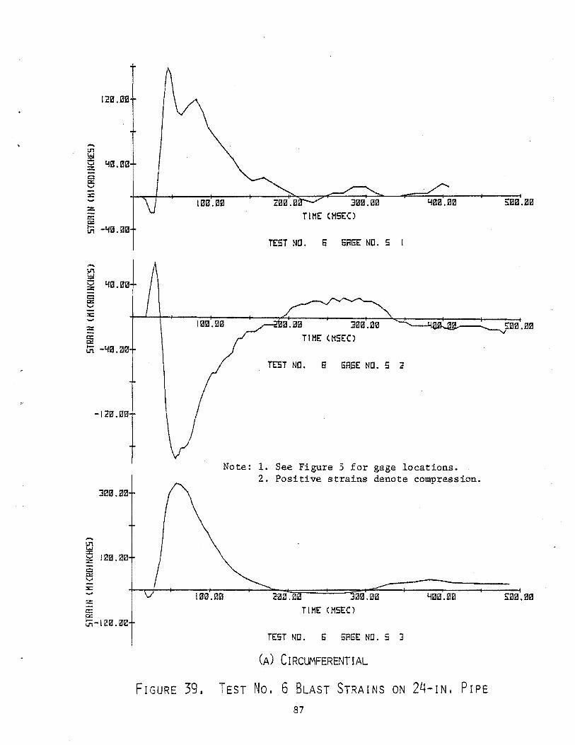
i r;~:um 0 a:: v :a:: .....

..... 1:!.1

-1211UI3

3313.133

0 13I:UU:l :z: 0

5 :a::

TIHE (115E()

TEST NO. 6 6RGE NO. 5

1313.fHil I:J.BB 3313.33 TIHE (HSE:O

TEST NO. E GAEE NO. 5 2

Note: 1. See Figure 5 for gage locations. 2. Positive strains denote compression.

.:~313.BB

TIME CMSEO

TEST NO. 6 GAGE NO. S 3

(A) CIRCUMFERENTIAL

FIGURE 39. TEST No. 6 BLAST STRAINS ON 24-IN, PIPE

87

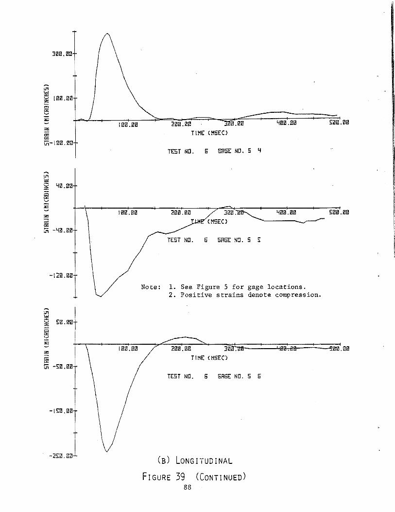
'""' L1'l !:::! c lBfUJa z c:::l 0:: v ::c

z c: 0::

tn-l flfl . fiB

..... L1'l w = l.!fi.BI:'! v z c:::l 0:: v ::c

::z: c: 0:::

tn -YB.kl121

..... L1'l w = v z c::::1 0:: v ::c ..... ::z: c: 0:::

-12B.!i13

S:B.fll:'!

tn -s:a .BB

-l~.!ilfl

l Bfl. Qllil

11:1fl.fll:1

::~nuu~ I.!Bfi.Bfl

TIM£ CMSEO

TEST NO . 5 tmGE NO. 5 y

YI:'!B.BB

5 GAGE NO. 5 s:

Note: 1. See Figure 5 for gage locations. 2. Positive strains denote compression .

TEST NO. 5 SAGE NO. 5 6

(B) LoNGITUDINAL

FIGURE 39 (CoNTINUED) 88

S:f!B.f!B

s:aa.aa

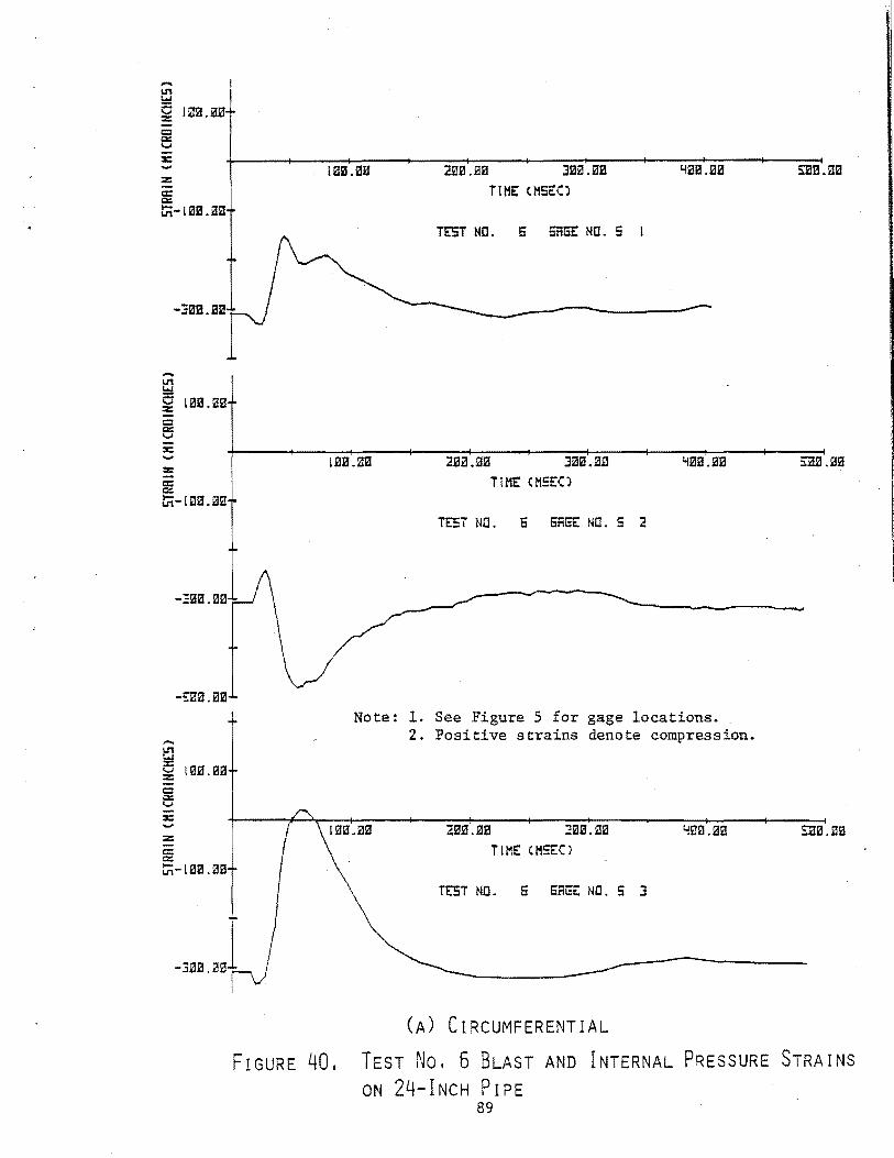
..... t

~ nm.a~J ::z:: c::::! e s:

-::aa.sa

..... ~ ~ li!UUIB c::::! e s:

HliU!B 2flB . aB Jilkl . BB SEI3.m!l

TIHE' CHS£0

TEST Nil . Ei 5REE' NO . 5 1

ZBB.Bil Jilii.ZB YliUUJB

TIME CM!:EO

TEST NC. E 6REE' NO. 5 2

Note: 1. See Figure 5 for gage locations. 2. Positive strains denote compression.

2BB.ZB TIME CHSEO

TEST NO. E 6RGE NO. 5 J

(A) CIRCUMFERENTIAL

FIGURE 40. TEsT No. 6 BLAST AND INTERNAL PRESSURE STRAINS ON 24-INCH PIPE

89

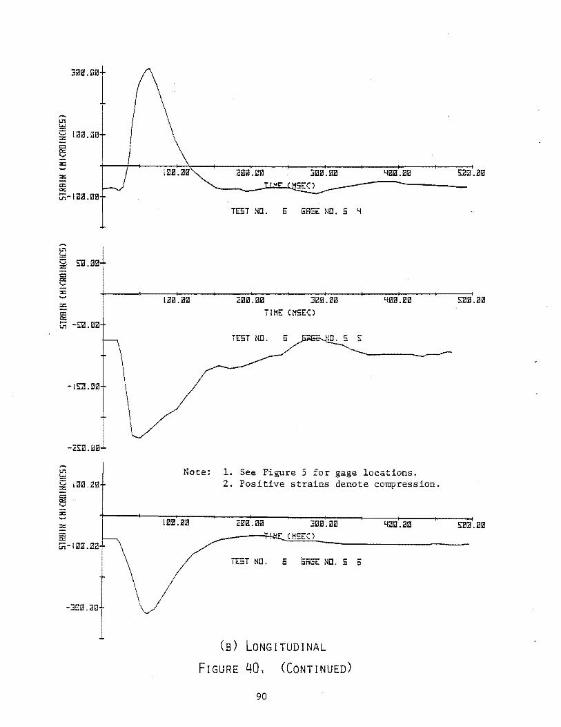
JBB.£B!

-IJ'I !:I Ci lt!B • .JEI :c

\ Cl

i Q::; ...... ::c

z = Q::;

t;;-103.BB

1 TEST NO. 6 GnE£ NC. S ~

-IJ'I !:I ~ SE.Ba Cl

e ::c ...... z 2B~.aa 30H.0B c.: TIME C!'!SEO Q::;

tii -s:B .fiE

TEST NO.

-<>a.e.l - I t;1 Ci

IBB.BBI :c c Q::; ...... :c ......

Note: 1. See Figure 5 for gage locations. 2. Positive strains denote compression.

I :c :J'!B. ma

taa.aai TEST NO • 6 SiiGF.: NO • S 6

-m •oj (B) LONGITUDINAL

FIGURE 40, (CONTINUED)

90

TABlE X. MAXIMUM STRAINS FROM BLAST LOADING ON 24-IN. PIPE

Charge Standoff r~~ Circumferential ~ (1. Longitudinal p1t;C

Test ~

Weight Q Distance Sl S2 -yd S3 11AtJ 84 s5 rd s6 No. (lb) \) (ft) (]..le:) (w::) (]..!E) (]..!E:) (]..le:) (]..le:) ~. ./ ~

1 \'~-·"- 15 lq~ 11 9.4 219 -268 352 360 -229 -309 1· ~~

2 )\.'1 5 6.0 856 -974 -933

3 \[.~ 5 6.0 708 -586 917 854 -615 -628

4 (ll\ 15 13.0 264 -214 537 588 -303 -786

5 ~.~~ 5 9.0 248 -219 404 454 -280 -492

6 \4."1 15 13.0 159. -175 330 390 -159 -243

7 \1.~ 15 13.0 150 -149 274 336 -183 -317

8 '{:J-\,. 15 6.0 -2800 1352 3815 5865 -1283 -6783

Positive strains denote compression

TABLE XI. COMBINED BLAST AND INTERNAL PRESSURE STRAINS

Circumferential Longitudinal

Test Sl S2 S3 S4 S5 86 No. (]..le:) (]..le:) (]..le:) (]..!E:) (]..!E) (]..!E:)

4 -405 -531 -342 513 -378 -861

5 -429 -534 -332 379 -355 -567

6 -335 -476 -348 315 -234 -313

7 -383 -470 -342 261 -258 -392

8 -2,875 -1,052 3,478 5,790 -1,358 -6,858

TABLE XII. MAXIMUM BLAST STRESSES ON 24-IN. PIPE

Charge Standoff Circumferential Longitudinal Test Weight Distance Stress Ssts~ Stress No. (lb) (ft) (£Si) (£Si)

1 15 9.4 10,600 . J ol1oo 10,800

2 5 6.0 29.200 1 28,000

3 5 6.0 27,500 )i~ 25,600

4 15 13.0 16,100 23.600

5 5 9.0 12,100 14,800

6 15 13.0 9,900 11.700

7 15 13.0 8,200 10,000

8 15 6.0 Beyond elastic limit

91

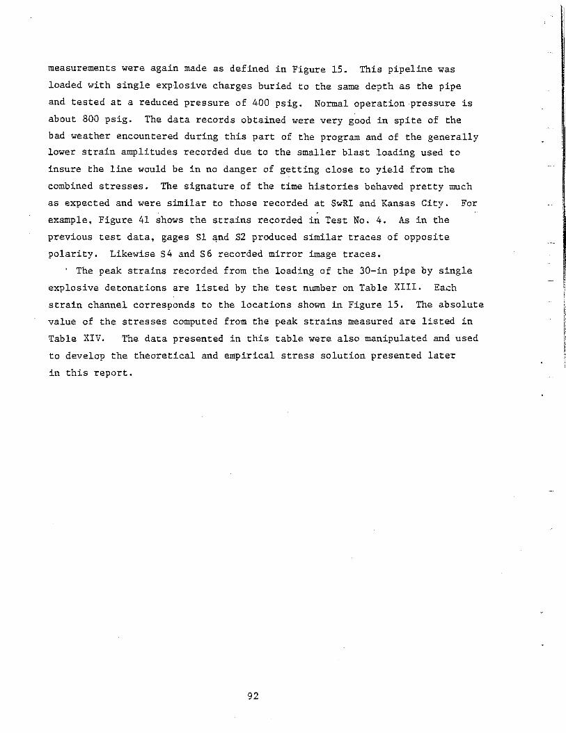
measurements were again made as defined in Figure 15. This pipeline was

loaded with single explosive charges buried to the same depth as the pipe

and tested at a reduced pressure of 400 psig. Normal operation pressure is

about 800 psig. The data records obtained were very good in spite of the

bad weather encountered during this part of the program and of the generally

lower strain amplitudes recorded due to the smaller blast loading used to

insure the line would be in no danger of getting close to yield from the

combined stresses. The signature of the time histories behaved pretty much

as expected and were similar to those recorded at SwRI and Kansas City. For

example, Figure 41 shows the strains recorded in Test No. 4. As in the

previous test data, gages Sl qnd S2 produced similar traces of opposite

polarity. Likewise S4 and S6 recorded mirror image traces.

· The peak strains recorded from the loading of the 30-in pipe by single

explosive detonations are listed by the test number on Table XIII. Each

strain channel corresponds to the locations shown in Figure 15. The absolute

value of the stresses computed from the peak strains measured are listed in

Table XIV. The data presented in this table were also manipulated and used

to develop the theoretical and empirical stress solution presented later

in this report.

92

•·

%

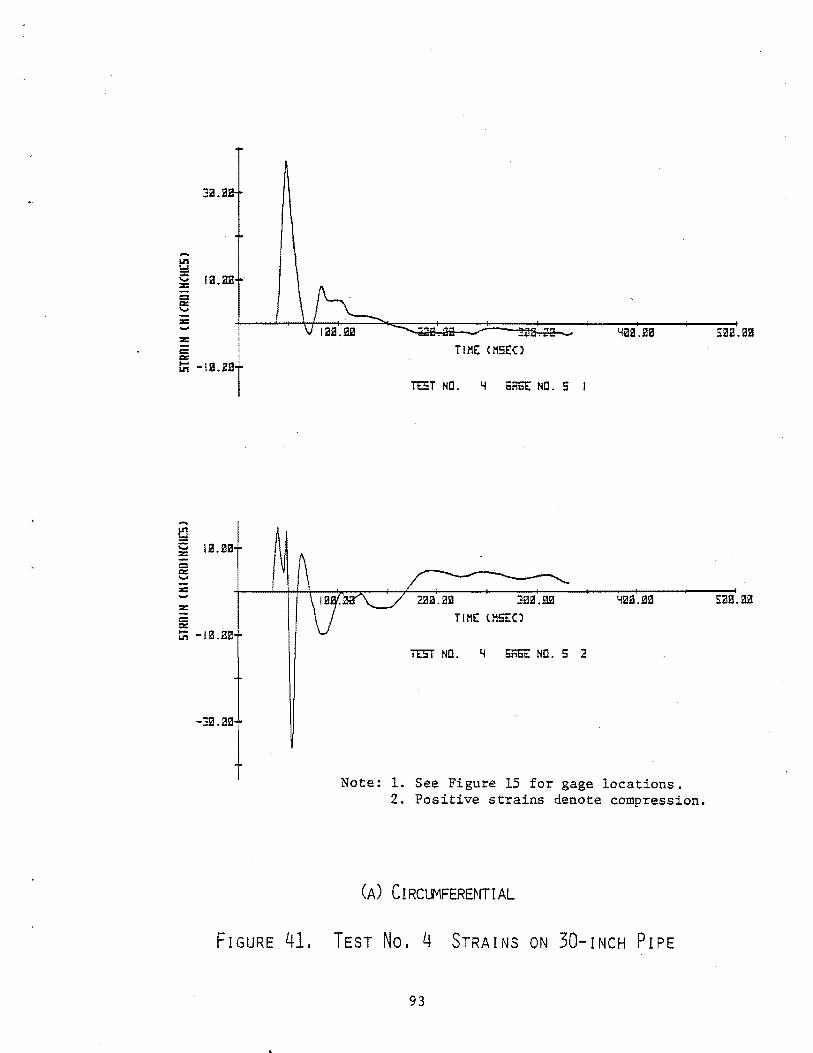
c: c::

3B.li1B

tii -lrl. ZB

t:l C i.B.EIB :z: c:l c:: .... :z:

%

c: c:: ::;; - 1 z . .aa

Tll1£ CMSEO

TEST NC. ~ 5MEE NC. 5 I

YBiUlB

TEST NO. ~ 5net NO. 5 2

Note: 1. See Figure 15 for gage locations. 2. Positive strains denote compression.

(A) CIRCLMFERENTIAL

FIGURE 41, TEST No. 4 STRAINS ON 30-INCH PrPE

93

S:lail..B!!l

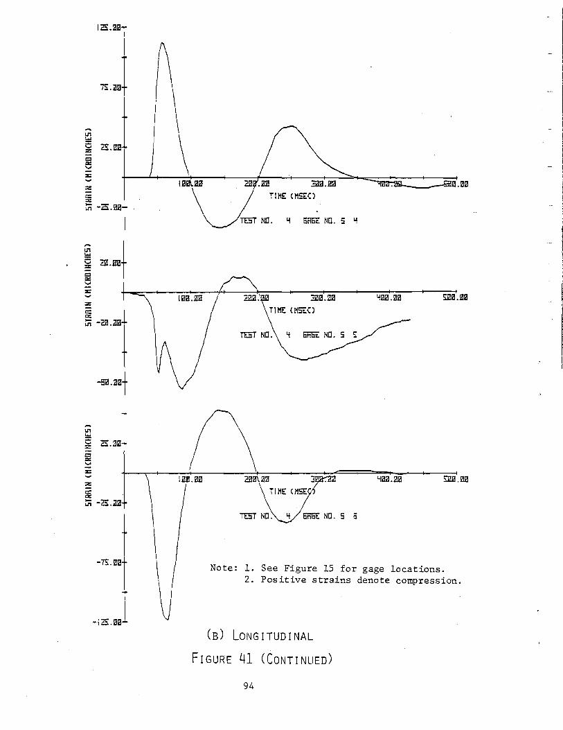
lc.ru!T l

1 U'1 ,J !:=! Ci :z: c 0:: ...... :c

:z:

a: t:n -2S. rul I

U'1 !:=! Ci 3UIB :z: c ct: ...... :c

:z: a: ct: t:n -CB .rul

-sum

...... ! U'1 ..... a 2S.aa :;;::

:z: a: 0::

t:n -c: .IDJ

-~.001

I

-io.lllll

~ \ \ lmlru!

TlHE Cl'ISEO

Y 6MEE NO. 5 Y

TEST NO. Y EREE NO. 5 6

Note: 1. See Figure 15 for gage locations. 2. Positive strains denote compression.

(B) LONGITUDINAL

FIGURE 41 (CONTINUED)

94

~j ,7~~

TABLE XIII. MAXIMUM BLAST STRAINS MEASURED ON 30-INCH PIPE

~ Charge Standoff Circumferential Longitudinal

Test 1 Weight &·, .. Distance '() Sl S2 Sl3 S4 S5 S6 No. ' (lb) (ft) c10 .-- (llE) (}.IE) (}.IE) (}.IE:) (}.IE) (f,IE)

---·-1 ~~.1 5 1,$1> 15 ~o-"' 101 -34 126 -88 -166

I

2 4 /,04 15 (,':.>

40 -31 73 -40 -80 t),(p

3 3 {,,';~

9 5·1-

251 -195 186 389 -141 -235 1~.~ ,, 4 ?Y·'~- 3 15 'fi·1 37 -36 39 112 -64 -123

TABLE XIV. MAXIMUM BLAST STRESSES ON 30-INCH PIPE

Charge Standoff Circumferential Longitudinal Weight Distance Stress Stress

Test No. (lb) (ft) (psi) (psi)

1 5 15 3,000 5,000

2 4 15 1,200 2,400

3 3 9 7,500 11,700

4 3 15 1,200 3,700

95

V. GROUND MOTION RELATIONSHIPS

Introduction

New empirical relationships were developed for predicting maximum.radial

soil velocity and displacement when buried explosive charges are detonated

in soil or rock. These relationships are needed because the ground motion

defines the forcing function applied to a buried pipe from blasting. In

addition, some state laws have a safe blasting criteria for any structure

(buildings, pipes, houses, etc.) which is based on limiting the maximum soil

particle velocity to less than 2.0 in/sec. Th{s statement does not say we

agree with the basis for such laws; however, these laws are used. The relation­

ships which will be discussed for explosive point sources are given by

Eq~ation 30, radial displacement, and. Equation 31, radial particle velocity.

p 1/2 X (__£_) R 2

0.04143 ( w 1.105 2 3)

c R = ------------~~~--~~~-1 5 w 0.2367

where

X

u R

w

p

c

pc

=

= =

-=

tanh • [18.24 ( 2 3

) ] pc R

3 w 0.8521 6.169 X 10- ( 2 3

)

c --------------~p~c~R=-~~---W 0.30

tanh [26.03 ( 2 3) ] pc R

maximum radial soil displacement

peak radial soil particle velocity

standoff distance

eXplosive energy release (use radio-chemical energy release for nuclear sources)

mass density of the soil or rock

seismic P-wave velocity in the soil or rock

atmospheric pressure

96

(30)

(31)

-·,

__ ; 1

Any self consistent set of units may be used in applying these relation­

ships for all terms; X/R (p /pc2) 112 , U/c (p /pc2) 1/ 2 , and W/pc 2R3 are 0 0

nondimensional. Experimental test data on explosive sources ranging from

0.03 lbs to 19.2 Kt (nuclear blast equivalency) will be used in subsequent

discussion to demonstrate the validity of these relationships. The data

used in substantiating the validity of these results cover nine orders of

magnitude in scaled explosive energy release, the quantity W/pc 2R3 from -11 -2 approximately 4.4 x 10 to 4.4 x 10 •

Major differences separate these empirical equations from others that

predict ground motions. This new procedure is not log linear; test results

cover more orders of magnitude, and a coupling term (pc 2/p ) 1/ 2 is divided 0

into the scaled displacement and velocity. The presence of atmospheric

pressure in the prediction relationships does not mean atmospheric pressure

is a physical phenomena influencing the result~ The quantity pc 2 is a

measure of the compressibility of the shock propagation media. Hence, the

quantity p is a standard (compressibility of air) and introduces empirically 0

relative compressibilities for different media such as soil and rock. This

point will be elaborated later.

Historical Background

Two different groups of ground shock propagation procedures have been

used in the past for empirical relationships interrelating charge weight,

standoff distance and ground motion. The approach generally used by

statisticians was to propose a propagation law of the form

where

A = is the peak amplitude for either velocity or displacement

n's = are constant exponents

K = is a constant

(32)

This format is popular because the logarithm can be taken of both sides to

obtain:

[ln A] = [ln K] + ~ [ln W] + nR [ln R] (33)

97

Because this equation is linear, a least squares curve fit can be made to

obtain the three coefficients ln K, nW, and nR. The weakness of this

statistical approach is that this format is assumed regardless of what

happens physically. The resulting equations are dimensionally illogicaL

A serious problem is the statistician's use of an incomplete expression.

Other parameters enter the ground shock propagation problem, especially

soil properties, which are ignored. Because these properties are ignored,

the definition of the problem is incomplete, and the results do not represent

a general solution.

Using the statistical approach, various investigators obtain different

results depending upon the amount and range of their data. Typical values

found in the literature[S-l5] have a range for ~ from 0.4 to 1.0 and for

nR from -1 to -2 with A as particle displacement or velocity. This situa­

tion arises because investigators use data from different segments of the

curve as given by Equations 30 and 31).

The second group of individuals, usually these associated with the

Atomic Energy Commission, present their results in the format:

U a

n 1/3 w

(-w-) R

n 1/3 X w

_x_a(-R-) wl/3

(34)

(35)

This approach is an extension of the Hopkinson-Cranz scaling law for air

blast waves, and is a dimensional version of a model analysis. If soil

properties such as p and c are treated as constants; and dropped from the

resulting pi terms in a model analysis, the dimensional versions as presented

in Equations (34) and (35) are obtained. An example of curve fits for

displacement and velocity to Equations (34) and (35) is given in Murphey.[lS]

= constant (36)

= constant (37)

98

..

Murphey's data were all obtained for chemical explosive detonations in

Halite (salt domes) and cover scaled charge weight over three orders of

magnitude. The authors certainly agree with Murphey and other AEC

investigators on using modeling principles. These curve fits will be

expanded by including data obtained over nine orders of magnitude and by

including an additional parameter.

Problems With The Conventional Modeling Approach

If the soil properties p and c are listed in a model analysis together

with the explosive energy release W, standoff distance R, and either of

the response parameters U or X, then two dimensionless pi terms are

obtained for either displacement or velocity as in the following functional

relationships:

X fx - =

R (38)

(39) u fu

w - = ( 2 3) c

pc R

Experienced modelers can readily see that with p and c considered as

invariant, these equations amount to Equations (36) and (37). No reason

exists to presume that the general but unspecified functional format given

by Equations (38) and (39) should be log linear. The functional format

can be obtained by nondimensionalizing experimental test data and plotting

the results provided the analysis is completely defined.

Figures 41 and 42 are plots of scaled deformation and scaled velocity

using limited amounts of test data for chemical explosive detonations.

The displacement data seen in Figure 42 come from only two sources,

References 15 and the test results obtained in this program at the SwRI

test site. Murphey (Reference 15) describes two types of Halite experiments.

In one group of tests, the soil is in contact with the explosive charge.

In another group of tests, 6- to 15-ft cavities placed an air gap between

the soil and the explosive charge. These tests described by Murphey called

"Cowboy" used 200, 500, and 1000 pound charges. The tests denoted by

circles in Figure 42 were conducted in this program at the SwRI test site.

99

ui 1

:

- 'V HALITE, NO CAVITY, AEC

A HALITE, CAVITY. AEC 0 0 ~0 0

u52 0 SOIL. NO CAVITY. SwRI 0 F oo -

. 0

0 0 0

ol¢o 0 0 0

0

1()3 00 0

..... -0 o o Oo

1- cP 0 00

1- 0 eeo

0 O'a ooo .0.

ui4 ..... co oo -'¥ 0~0

.0. 1-

~ 4 X 1--R-

~ ~ 0

.0.

105 1":- '¥ -

'¥ .0. '¥ . '¥

.0.

'¥ ~ .

'¥ .0. <l. w

'¥ 106 - f1

'¥ -- If" '¥

ft .0.

'¥ '¥

'¥ a '¥ '¥

107 A A .. -A

!-.0.

A .0.

.0.

108 I

Hi9 ui8 107 106 J65 Hi4 10

3 Jti2 Hi1

P 'R3 s

FIGURE 42. GROUND DISPLACEMENT IN RocK AND SOIL No CouPLING 100

All of these tests were in silty clay soils with various moisture contents.

The charges ranged from 0.03 to 1.00 lb of explosive. Although more data

could be plotted in Figure 42, correlation will not occur. Obviously some

phenomena are present in Figure 42 which are not reflected in a solution as

given by Equation (38).

The same lack of correlation which became apparent in Figure 42 for

displacement is also apparent in Figure 43 for peak particle velocity.

An additional compilation of data not contained in Figure 42, has been

included in the Figure 43 velocity plot. Harry Nicholls, et al [16]

summarize velocities obtained from blasting in stone quarries. If only

single explosive source detonations are used in this compilation, approxi­

mately 50 data points can be obtained for a variety of charge weights, site

locations and standoff distances. In addition to this new data, the peak

particle velocity data corresponding to halite, both with and without cavity,

and soil tests are included in Figure 43.

Although the data in both Figures 42 and 43 fail to correlate, they do

show some systematic tendencies. Increasing values of W/pc2R3 result in

increasing values of scaled ground motion, and the slopes associated with

the various data points are almost identical. The figures infer that some

phenomena not included in the analysis should be added. In particular, both

figures indicate that a different coupling must exist between different

soils or rock and the explosive source. Obviously the poorest coupling

exists when an air gap or cavity separates the transmitting media from the

explosive source as in some of Murphey's halite experiments. Figures 42

and 43 show that the resulting ground motions are less for experiments with

a cavity in halite. However, a weak rock, such as halite, should have a

better coupling than soil when both are in contact with explosives. Figures

42 and 43 indicate that ground motions are greater for detonations in rock

than for similar detonations in soil. From these detonations, a coupling

tena could be added to Equations (38) and (39) to achieve better correlation.

Addition Of An Impedance Term

The term which was added to either the scaled displacement X/R or the

scaled velocity U/c terms was the square root of the soil compressibility

relative to a standard compressibility, the compressibility of air. This

101

u c

102

0

\1

6.

103 0

ROCK, NO CAVITY, DENVER MINING RESEARCH CENTER

HALITE, NO CAVITY. AEC

HALITE, CAVITY, AEC

SOIL, NO CAVITY, SwRI

<>

v

vv v

v

t..

~

v v

a l!t.t,.

t..t:;. t..

t..

t..

!:A

0

8<9 0 0

0

w

FIGURE 43. PARTICLE VELOCITY IN RocK AND SoiL No CouPLING

102

quantity /pc2/p was divided into the nondimensionalized ground motions

to obtain the f~nctional equations, (40) and (41).

X p 1/2

(-0-) R 2

PC

U p 1/2

(.....£.._) c 2 pc

=

=

2 1/2 2 1/2 Creation of the terms (X/R) (p /pc ) and (U/c) (p /pc ) was based

0 0

entirely on empirical observation. A functional format could also be

created by plotting the dependent and independent variables in Equations

(40) and (41). In addition to using the no cavity data presented in

(40)

(41)

Figures 42 and 43, the ground motion data obtained in this program at the

Kansas City and Kentucky test sites, and additional AEC data were plotted

using results from some buried nuclear detonations. The cavity test results

in halite were not replotted because this empirical approach does not

account for ground shock propagation when charges are placed in cavities.

The AEC data, which were also plotted, come from References 17 and 18.

Both soil displacement and maximum particle velocity were reported in

Reference [17] on Project Salmon, a nuclear blast yield of 5.3 kilotons;

hence, this data will appear in both scaled velocity and displacement plots.

Reference [18] is a summary of displacement and acceleration, but not velocity,

for numerous large AEC buried detonations. Maximum scaled displacement data

are included for such projects as a 19.2 kiloton detonation named Blanca, a

77 ton detonation named Tamalpais, a 13.5 ton detonation named Mars, a 30

ton detonation named Evans, and a 5.0 kiloton detonation named Logan. The

writers in References 17 and 18 are not clear; we believe they are quoting

equivalent blast yields for nuclear detonations. Test results indicate

that for buried nuclear detonations the radio chemical yield is more appro­

priate than the equivalent air blast yield. The radio chemical yield is

twice as great as the equivalent air blast yield, so all of the blast yields

listed in this paragraph were doubled before plotting any data points. In

addition, the energy W had to be converted to foot pounds of energy by

103

multiplying explosive weight by 1.7 x 10+6 ft-lbs/lb, or the appropriate

conversion factor, so the quantity W/pc2R3 would be nondimensional. The

density is a bulk mass (not weight) density, a total density of the media,

and c is the seismic P-wave propagation velocity .. Other soil data might·

exist, but only results in which c was measured and reported could be used

in this evaluation. Obviously, the gas industry has little interest in

nuclear explosions, however, the inclusion of this data emphasizes the broad

applicability of these results.

Figures 44 and 45, respectively, are plots of nondimensionalized dis­

placement and nondimensionalized velocity as given by Equations (40) and

(41). Because the data appear to collapse into a unique function, these

results give a graphical solution. Scatter does exist; however, no experi­

ments or test site appears to Yield systematic errors. The range in any test

condition is larger than ranges in

reports. The scaled charge weight

magnitude from approximately 4.4 x

any previous ground shock propagation 2 3 W/pc R ranges

-11 10 to 4.4 x

over nine orders of

10-2 . The charge weight

itself ranges from 0.03 lb of chemical explosive to the radio chemical yield

of 38.4 kilotons in Blanca, a factor of over one billion. The range in soil

or rock densities is small because nature offers only a/small variation, but

the wave velocity c ranges from approximately 50~ fps to 15,000 fps, a factor

of 30. The soil data measured in this program are at much closer standoff

distances to the charge than other results, but the transition does seem to

be a continuous one.

The continuous lines placed through the data in Figures .44 and 45 were

presented as Equations (30) and (31). Both are the result of "eye-balling"

curve fits to the test data. One standard deviation for the test results

about either line is approximately ±50%. Although straight lines can be

curve fit to segments of the results in Figures 44 and 45, the rate of

change for either X or U with respect to either W or R varies dependent upon

the scaled charge weight W/pc 2R3 • These variations are reasonably close

to those given by others and discussed in the historical background

presented earlier in this section. Closest to the charge where these slopes

are greatest, are slightly larger exponents than those which were previously

reported; however, the earlier observations did not include data obtained in

this study.

104

1-' 0 Vl

112

(f)(:,~)

10-ll

S YMOOL I'ROJECI 'il COWBO'I' o SwRI X SAlll'£lN C. BlANCA A TAMALPAIS + MARS 0 EVANS 0 lOGAN lt SwRI Q . SwRI- KY

CHARGE SIZE 200 lo IOOJ lb

0.03 lo 1.0 lb 5.3 kf

19.2 kf 111

13.5 T lOT

500J T 5 to 15 lb 3 lo 51b

FIGURE 44.

0

10-l I0-6

w pc2Rl

1,...------------:r-rTTTTr- -.,----.-rTTT l"ll

c.

10-s

"

0

" lt

(.X.)(.!J!_}I/2 0.04I43 ( W } 1.105 R pc2 • ~

lallllu[ 18.24 (-w }0.2367] pc2Rl

I0-4

CouPLED DISPLACEMENT IN RocK AND SoiL

102

I-' 0 0\

U ( Po c pc2

S VMBOL PROJECT '<l COY/BOY o SwRI X SALNON 0 BUREAU ol MINES () SwRI Q SwRl- KY

CHARGE SIZE 200 lo 1000 lb

0.03 lo 1.0 lb 5.3 kT

VARIOUS 5 lo 151b 3 to Sib

I I !!ttl I I 10-10 I I 1 t I I pi ~-u·~~~~~~~~~~~~~~tU!li~--L-1~1-J I

FIGURE 45.

1lt v

()

0

0

w )0.8521 6.169 X l0·3(;z;l

(UX~)11

: w )0.3] c pc2 lanh [ 26.03 ( pc2R3

I I I I i! I """: __ ....J..._Jic..J!...l.l .ll II t i1 I I ---::::1-LI LI~I~IJ~I,.._LI-'-'-''";:c.o--'--'-'""-":.;;--''-'-'""'"",--"-'-'-'''': I I I II ltl I I 1 • I I tJ I I I I I f I t! I t 1 I ) I I I If

w pc2R3

CouPLED PARTICLE VELOCITY IN RocK AND SoiL

Discussion Of Coupling Term

The term (pc2/p )

112 which is divided into the scaled velocity term

0

U/c and scaled displacement term X/R is an empirical factor which seems to

work. The fact that the compressibility of the soil (pc 2) is proportional

to a modulus of elasticity (E) is related to the compressibility of air,

does not mean that atmospheric pressure is actually a parameter physically

entering this problem. If these ground shocks were to be propagated on

the moon where essentially no atmosphere exists, the amplitudes of the

response would be finite rather than infinite as inferred by this solution.

The atmospheric pressure p was just a convenient constant which non-2 0

dimensionalized pc .

Perhaps p enters pore pressure considerations and actually does belong 0

in these calculations; however, this is doubtful. Other parameters which

have the dimensions of pressure could be considered, but those parameters

would essentially have to be constants in all soils. Examples of possible

substitutes for p could include: (1) n (the density times the heat of 0

fusion) if one believes significant amounts of energy are dissipated in

phase changes, (2) pc e (the heat capacity times an increase in tempera-p

ture) if thermal heating is important, (3) the energy per unit volume (area

under a stress-strain curve) in a hysteresis loop if material damping is

important, and (4) others or combinations of all of these effects. No

satisfactory explanation has been drawn. The point which makes all hypo­

theses difficult to accept is that p or its counterpart must be essentially 0

constant in all soil and rock tests. A numerical value other than 14.7 psi

does not invalidate this solution; a different constant only translates all

curves.

Ground Shock Around Line Sources

Sometimes more than one buried charge is detonated simultaneously. If

many equally spaced charges are strung along a line as in explosive ditch

digging, the ground motion must be predicted for a line rather than point

source. The major difference in these line solutions is that the term

W/pc 2R3 becomes W/~/pc2R2 where W/~ is the energy release per unit length

of line. The ground motion equations in functional format then become:

107

X R

u c

p 1/2 (-0-)

2 pc

p 1/2 (-0-)

2 pc

= fx (w/ t ) 2R2 pc

(W/£ ) 2R2 pc

(42)

. (43)

Experimental test data were needed to complete the functional format

for these line source·equations. Not every experiment is applicable because ··

these solutions are for infinitely long lines. The standoff distance

cannot be much greater than the length of the line, and must be large

relative to the spacing between successive charges if an infinitely long

line source is to be approximated. In this program a large amount of line

source displacement and velocity data were obtained for experiments in soil.

Reference 16 supplements the velocity data (no displacement data) at an

en~irely different range of scaled standoff distances with measurements at

the Littleville Dam construction site. Although other multiple detonation

data is reported in Reference 16, it cannot be used as line sources because

either successive charges were delayed or the standoff distances were much

larger than the length of the explosive train.

Figure 46 for radial soil displacement from line sources and Figure 47

for maximum particle velocity from line sources present this data in the

formats suggested by Equations (42)and (43). Straight lines have been curve

fitted to this data. The functional formats are given by Equations (44) and

( 45).

X p 1/2

(W/fJ. .) 1.125

(-0-) = 0.0792 (44) R 2 2R2 pc pc

p 1/2 1.010 u (-0-) 0.7905 (W/£ ) ( 45) = c 2 2R2 pc pc

108

N --.............. N

'-' Q. -0 Q. .............

c:::: N -X

10-4

w~s

X/R(pJp c2 ) 112 • 0. 0792( W/ J.fp c2R 2 )l.l2S

e SwRI DATA

•

• • • • •

• • •

•

FIGURE 46. RADIAL SOIL DISPLACEMENT FROM LINE CHARGE DETONATIONS

109

U/c (p0/pc2) 112 " 0. 7905(Wil/ pc2R2) l.OlO

e SwR I DATA

~ BUREAU OF MINES DATA REFERENCE 16

•

•

FIGURE 47. MAXIMUM SoiL PARTICLE VELOCITY FRoM LINE CHARGE DETONATIONS

110

Ideally, more data would be available over a wider range in scaled charge

weights and at several sites so more confidence would exist in Equations

(44) and (45) as prediction equations. The range of validity is not as

great, and c was estimated rather than measured at the Littleville Dam site.

Equations_ (44) and (45) although helpful, should be given only tentative

acceptance.

Further Approximation For Displacement

The results presented in this discussion are those which will be used

to determine the load imparted to a buried pipe. Equations (30) and (31)

for buried point sources and Equations (44) and (45) for buried line sources

are more accurate than other curve fits which were discussed earlier in this

section. One further simplification can be made as an approximation to Equa­

tion (30). Over a limited range in i 3 of from 1 x 10-7 to 4 x 10-2 , Equa-pc R

tion (46) is the most accurate log-linear relationship.

X R

p 1/2 (-0-)

2 PC

= 0.025 w ( 2 3) pc R

(46)

Equation (46) is a fairly accurate prediction equation. When in error,

it generally overestimates the displacement X; thus, is conservative. At w -7 values of 2 3

less than 1 x 10 , Equation (46) begins to underestimate pc R

the displacement, and becomes dangerous. For conventional pipeline applica-W -7 tions, the use of Equation (46) for values of 2 3

less than 1 x 10 presents pc R

no problems as the associated scaled displacements are too small to threaten

a pipeline. Only if blasting charges exceed 100 tons, as in large nuclear

simulations, would the use of Equation (46) present problems. Equation (46)

is a much simpler equation to use than Equation (30) with its hyperbolic form. w All of the blasting performed in this program was for values of 2 3 greater

4 pc R than 1 x 10- . This observation means that the simpler form given by Equation

(46) can be used. Figure 48 shows Equation (46) plotted versus the test re­

sults from Figure 44, and indicates that these conclusions are correct. In

analytical derivations, Equation (46) rather than Equation (30) is used. Many

simplifications will result in the final solution because of this approximation.

111

!-' !-' N

{f}~c~} Ill

:"

~ .ffiQlKl CHARG£ SIZE v COWBOY zm to 1000 lb 0 SwRI 0.03 to 1.0 lb X SALMJH 5.3 kT Q BLANCA 19.2 kT A JAMIILPAIS 171 + rMRS 13.5 t 0 EVANS lOT 0 lOGAN 5000 I U/!:f~ (t

0 SwRI S lo 15 lb

0

0

0

a

Q )(

0

0

)f( 0

)(

10·10 tli9

FIGURE 48.

108 I0-1 106

w pc2R3

Jo5 ui4

EQUATION 46 COMPARED TO DISPLACEMENT TEST DATA

-~=~--~~~~~~~--~--~~-s~~~~~

VI. ANALYTICAL DERIVATION OF PIPE STRESS FORMULA

Introduction

The ground motions predicted in the previous chapter impart a shock

loading to a buried pipe. Basically, this load takes the form of an impulse

imparting kinetic energy to a buried pipe. This kinetic energy is dissi­

pated by changing to strain energy. Significant strains were recorded and

are reported in Section IV in both circumferential and longitudinal

directions. The purpose of this analysis is to derive an approximate form­

ula to interrelate maximum pipe stress in both directions to the various

pipe, soil, and explosive parameters of importance.

The solution which follows uses both approximate analysis procedures to

interrelate variables and empirical test results to develop the final func­

tional format. Only elastic analysis procedures will be used because it is

considered unacceptable to permit any stress to exceed yield in a pipeline.

All pipe stress data used in this derivation comes from the data reported

in Section IV. These data are used to both derive and evaluate the accuracy

of the resulting expressions.

Predicting Impulse Imparted to Pipes

Before structural calculations can be made, the impulse distribution

imparted to a pipe from a ground shock must be estimated. This load becomes

the forcing function needed in structural calculations.

The side-on pressure and subsequent impulse must be determined without

a pipe present before the impulse imparted to a pipe can be determined.

Fortunately, soil particle velocity and displacement, predicted in Section V,

relate directly to free-field or side-on pressures and impulses. To cal­

culate pressure from particle velocity, we use the Rankine-Hugoniot rela­

tionships for conservation of mass and momentum. For a stationary coordinate

system with a shock front moving at velocity V, these equations are:

-p V = p (U - V) s a

Ps vz = P + P (u - V)z s a

113

(47)

(48)

where p is the density behind the shock front and p is the side-on a s

overpressure. Multiplying both sides of Equation (47) by (U - V) and then

substracting the new Equation (47) from Equation (48) gives:

(49)

Equation (49) states that peak side~on overpressure is the product of

soil density, shock front velocity, and peak particle velocity. In a fairly

imcompressible medium such as soil with its massive particles, the shock ··

front propagation velocity V very rapidly decays to c. Substitution of c

for V is a common practice in hydraulic shock studies and would appear to

be equally valid in soil. This final substitution yields the equation which

will be used to relate side-on overpressure and particle velocity.

P = p c u s s

(50)

Either Equation (46) for point sources or Equation (44) for line

sources can be substituted into Equation (50) to determine p . To deter­s

mine the side-on specific impulse i , we will treat p and c as constants s s and integrate Equation (SO). Because the time integral of pressure is

impulse and the time integral of velocity is displacement, integrating

Equation (50) gives:

i s

(51)

Equation (51) also can be used for values of X from either point or

line charges. Next, the distribution of impulse imparted to a buried pipe

by side-on impulses must be estimated. Figure 49 shows a pipe loaded by

an assumed distribution of applied impulse. It is known that at the top

and bottom of the pipe, the applied impulse will be i • Also, that at a s

lower limit at the front of the pipe the impulse will equal at least 2 i . s

Between the top and front edge of the pipe, some distribution will exist

which is not known. Therefore assuming some distribution, a convenient

mathematical expression, Equation (52), which reaches the correct limits,

was selected.

114

0 < e < n 2

i = is [ 1 -2 ~ 9

) tor 0 > a > - ~

FIGURE qg, AssuMED DISTRIBUTION oF IMPULSE IMPARTED TO A PIPE

115

BACK

i = is ( 1 + ~8 ) for 0 < 8 < ;r/2 (52)

The back side of the pipe will also be loaded by the shock wave dif­

fracting around the pipe. At 8 = -;r/2, on the very rear surface of the

pipe, the impulse could very easily exceed i ; however, no one knows the s

exact magnitude. This was solved by assuming that the applied specific

impulse equals (1 + m)is at the back of the pipe where m is some number be­

tween 0 and 1. Experimentally measured stresses will be used later to assign

a constant numerical value to m. The distribution of impulse over the back

surface of the pipe is similar to that used over the front surface and is

. _ . (l 2 m 8 ) ~ - ~ -s iT

for 0 > 8 > -'TT/2 (53)

A minus sign appears in Equation (53) because the angle 8 is measured in a

negative direction.

The total impulse I imparted to a pipe by the specific impulse distri­

butions given in Equations (52) and (53) can now be computed. For a dx

differential length of pipe, this impulse is given by:

;r/2 I

(dx) = 2 J (sin 8)r d8 - 2

0

Or, after simplifying algebraically:

I (dx) =

4(1 - m) . ~

iT s r

Performing the required integration gives:

;r/2

f 0

;r/2

f 0

e sin 8 d8

I = i (1 - m) i r (dx) iT s

116

(sin e)r d8

(54)

(55)

(56)

Equation (56) is the total impulse imparted to a ring segment. This

equation can also be written as:

where

I = CD is A

A s 2 r (dx), the projected area

2 CD=; (1-m), a diffraction coefficient

(57)

Equation (57) states that the total impulse is the specific impulse times

the project areas times a constant diffraction coefficient. The constant

diffraction coefficient will be determined empirically from test results.

Determining CD amounts to determining m, as they are both related through

the definition of CD. It should be emphasized that CD as created in this

analysis is not a drag coefficient and is specifically called a diffraction

coefficient because it is associated with a diffraction process.

Derivation of Pipe Stress Formulae

To determine pipe stresses, calculate kinetic energy and strain

energy. The first of these, kinetic energy (KE), is given by:

2 I2 9../2

I2

L L f KE = mV == -= 2 2 0 2m 2m

pipe pipe 0

(58)

Substituting Equation (57) for I and assuming that an effective mass of

earth from the center of the charge to the center of the pipe moves with

the pipes gives the result:

9../2

KE = f 0

c~ i! (2r)2

(dx)2

p (2r) R (dx) s

(59)

This assumption of a large effective mass of earth moving with the pipe

causes the mass of the pipe itself to be insignificant. It is based on

117

empirical observations made during pipe tests reported in Section IV. For

bending in a ring, the fundamental natural frequency w is given by:

(60)

where 1 3

J = 12 (dx) h , the second moment of area

~ = the mass per unit length

When it was assumed that the mass of earth was p (dx) R, rather than the s

mass of the pipe~ substituting this mass in Equation (60) and computing

the period T from the frequency w gave:

(61)

Calculated periods using Equation (61) agreed well with observed dur­

ations in the pipe strain records on early model tests, as shown in

Table XV. These strain records also showed pipe ovalling; hence, inferring

that pipe bending is a correct mode of response.

TABLE XV. MEASURED DURATIONS AND COMPUTED PERIODS

Test Observed Durations Calculated Periods No. (m.s.) (m. s.)

1 16 11.7 2 11 11.7 3 13 11.7 4 25 31.6 5 35 34.8 6 36 34.8 7 71 66.8

If we now return to Equation (59) and perform the required integration,

we obtain:

KE (62)

118

Substituting Equation (51) for i in Equation (62) finally yields: s

2 2 2 CD ps c r fL X

KE=--"--.;;_,----R

(63)

Next, the strain energy SE must be calculated because of the pipe

responding in either a longitudinal bending mode or a circumferential mode.

For longitudinal bending, this computation is done by assuming a deformed

shape given by:

where

Y .. ( 'ITX) = w0

cos T

W = mid-span deformation 0

t = total length of the deforming pipe

Differentiating Equation (64) twice and substituting into the elastic

moment-curvature relationship gives:

d2 y 'IT2 EJ W o ( ) M = -EJ _d_x_2_ = --t"=-2_;;;.. cos 'ITt

But the strain energy is given by:

SE = 2

JL/2

J 0

M2

dx 2 EJ

Substituting Equation (65) into Equation (66) gives:

t/2

f 2 ('ITX) cos T dx

0

119

(64)

(65)

(66)

(67)

Which after integrating gives:

rr4 EJ w2 SE = ----0

"-

4 t3

. (68)

Next we wish to substitute for J and w • The second moment of area J 0

for a pipe is given by:

(69)

Substituting (r.+h) for r , this becomes: ~ 0

J = (70)

Using the binomial expansion and retaining only the first two terms because

h/r. is small gives: ~

(71)

Equation (71) reduces to:

(72)

The deformation w is related to the maximum stress by substituting into: 0

M c max cr = max J

(73)

But M occurs when the rrx 1.0 in Equation (65)' hence: max cosT equals

2 EJ 1T w

0 r cr = max t2 j

(74)

120

Which gives, when solved for w: 0

(J max

w = ----0 ·iE r

(75)

Substituting Equations (72) and (75) into Equation (68) finally gives the

longitudinal strain energy:

SE long.

cr 2 r h t 'IT max = - ----"----4 E

(76)

If it is assumed that the pipe goes into an ovalling bending mode as

was indicated by the recorded strains and by the calculated and observed

durations associated with vibrating pipes, the strain energy in the circum­

ferential direction is computed from an assumed deformed shape given by:

y = w cos 2e 0

(77)

The elastic bending moment, as computed from two derivatives of Equation (77),

is:

d2 y 4 EJ w M = -EJ = ----~2~

0 cos 2e r

2 de

2 r

The strain energy SE is given by:

'IT/4

SE = 8 f 0

M2

r de 2 EJ

Which, after substitution of Equation (78) into Equation (79), yields:

64 EJ w2 0 SE = ---:::---

'IT/4

f 0

121

2 cos (2e) de

(78)

(79)

(80)

Integration of Equation (80) gives the result:

8 1T EJ w2

SE = ----;;:-..;....0

3 r

(81)

Substitution of the maximum moment from Equation (78) when cos 26 equals

1.0 into Equation (73) gives:

Or, after solving for w: 0

4 EJ wo h/2 crmax = 2 T

r

2 cr r - .:::m:.:::a;::x;___ w = o 2 E h

(82).

(83)

The second moment of area J in the circumferential direction is given by:

(84)

Finally, substituting Equations (83) and (84) into Equation (81) gives for

the circumferential strain energy:

2 cr

1T max r h t S E = - _;;;;;::;;:.::......;;;.....~...;,.

cir 6 E (85)

Approximate solutions which interrelate the variables are obtained by

equating the kinetic energy, Equation (63), to the strain energy, Equation

(76) for longitudinal stress or Equation (85) for circumferential stress.

This computation gives the result:

Or:

cr2 CD2 ps c2 X2 (r £) 1T long h ( r £) = _,;;;;,_..;;..__ ____ _ 4 E R

cr long

122

(86)

(87)

Similarily, this procedure for circumferential stress yields the result:

6 CD E ps c X (

2 )112

1/2 1/2

(88) a . c~r = -1T- hl/2 Rl/2

Notice that in Equation (86) the quantity (r 2) on the strain energy

or left hand side of the equation cancels with (r 2) on the kinetic energy

or right hand side of this equation. This observation means that the stresses

will be independent of both the pipe length 2 and the pipe radius r. Static

analysis procedures do not yield this conclusion, and cannot be used to

draw valid conclusions in this dynamic problem. Dynamically, this solution

infers that doubling the radius r or size of the pipe doubles the kinetic

energy imparted to the pipe; however, this process doubles the amount of

material available for absorbing the input energy through strain energy.

The net result is that the pipe radius r cancelsout of the analysis and the

stresses are independent of pipe radius. The experimental data obtained in

this program on 3-in, 6-in, 16-in, 24-in, and 30-in diameter pipes will be

used later in comparisons which uphold this analytical observation.

The other major observation which should be made concerning Equations

(87) and (88) is that in both orthogonal directions the maximum stress

appears (

El/2 pl/2 c X) to equal the same quantity h112 : 112

times a constant which

differs for maximum circumferential stress a . and longitudinal stress c~r

a • This observation suggests that the final solution can be obtained long

by two plots, one for circumferential stress of a . c~r

and the other for

This procedure is precisely the one which was followed to develop the final

quantitative functional formats for predicting pipe stresses from buried

detonations.

123

Use of Data to Complete the Solution

In Section IV, pipe stresses from buried detonations are reported for

tests at SwRI, Kansas City, and in Kentucky. Experiments were conducted

using both line and point sources for explosive charge sizes varied by

greater than 2 orders of magnitude. All of these stress results are tabu­

lated in Tables IX, XII, and XIV from Section IV. These results are used

to empirically complete this derivation pecause formuli are needed in terms

of charge size rather than in terms of soil displacement. Equation (46)

from Section V was substituted into Equation (88) to obtain:

(J • c~r

lEw (89)

Equation (89) is nondimensional; however, it was written in a dimen­

sional format because R is inches and W is in-lbs of energy release and is

not very convenient for users in the field. Using the quantity (n W) as

equivalent lbs of AN-FO in place of an energy release, substituting 14.7 psi

for p , and making the appropriate substitutions so R would be in feet, E 0

in psi, and h in inches gives:

o . (psi) c~r

IE (psi) [n W (lbs AN-FO)] = [333.8 CD] /h (in) [R (ft)]2.5

(90)

Now plot the left hand of Equation (90) against the right hand side of

this equation. Figure 50 is this plot with the open symbols, the points

for a single explosive source. The shaded symbols are the test results

for line sources which will be discussed later. The line through the data

in Figure 50 has a slight curve but if the straight segment was associated

with the smaller values of crcir' it would have CD in Equation (90) equal to

0.1394 so Equation (90) could be written as:

a (psi) = [46. 53] IE (psi) [n w (lbs AN-FO)] v'h (in) [R (ft)] 2 ' 5

124

(91)

"cir (psi)

1000CO~--.--.-.~~~~---.--~~~on----~~~~~~~~

0 1000 s • 0. 46

LINE • 6" SwRI LINE • 3" SwRI POINT o 24" KC POINT ~ 16" SwRI POINT o 6" SwRI POINT ¢ 3" SwRI POINT 0 30" KENTUCKY

100 100 1000 10000 100000

69.76 vr(~w) 46.53 ff (nw) or

Vh R 3/2 Vh R2.5

FIGURE 50. CIRCUMFERENTIAL PIPE STRESS

125

The symbol a has been substituted for the maximum circumferential stress

cr . in Equation 91 because cr only equals a . for values of a less than c1r c1r

2675 psi. For larger values of cr, a . almost equals cr but not quite. The c1r

line actually drawn through the data points in Figure 50 is given by: ·

cr . c1r

c . = 1.0 cr c1r for cr < 2675 psi

= 21. 7 0' 0. 7 40 47.55 a 0 •584 for o > 2675 psi

(92a)

(92b)

The fact that the line curves in Figure SO is not distressing. The

analytical solution was created by assuming a deformed shape. In addition,

it is assumed that other modes of response do not occur and that the deformed

stlaped does not change with the intensity of the loading. Any or both of

these effects would cause transitions which have been handled in this solu­

tion by using empirical observation.

Experimental tests on the 3- and 6-in diameter pipe also used explosive

line sources. These data points are the shaded symbols in Figure SO. Equa­

tion (88) applies to line or point explosive sources, however, a different

ground motion relationship must be used in substituting for ground motion X.

For the point source solution we used Equation (46) as an approximation for

the more complex Equation (30), and substituted Equation (46) into Equation

(88) to eventually obtain Equation (91). Similarly for a line source solution,

we wrote Equation (93) as an approximation to the more complex Equation (lS).

1/2

= 0.0375

Given that a series of equal weight charges are spaced in a straight

line with an equal gap between each charge and are detonated, then a

(93)

line source solution is applicable if ~ (the length of the explosive line)

is greater than 2/3R and ~ is also less than NR. Equation (9] for a line

source was then substituted into Equation (88) and the proper dimensional

substitutions were made to obtain the following dimensional equation.

126

a (psi)= [69.76] IE (psi) [( ¥- lbs f'tFO) J

lh (in) [R (ft)]l. 5 (94)

Equation (94) is the line source counterpart to Equation (91) for point

sources. All of the observations made about Equation (91) pertain to Equa­

tion (94). For values of a less than 2675 psi, the quantity a in Equation

(94) for a line source equals a .. c1.r For large values of a the solution for

the line source also diverges slightly from Equation (94) as it did for

point sources. Hence, Equations (92) pertain to either point or line

sources provided the correct equation for a is applied.

In addition, to predicting circumferential stress, we also need to

predict maximum longitudinal stress from blasting a1

• Because Equation ong

(87) for longitudinal stress is similar to Equation (88) for circumferential

stress except for a constant, longitudinal stress a1

should plot as only ong

a slightly different function of cr. Figure 51 is this longitudinal stress

plot using the longitudinal stress test data also summarized in Section IV.

Both point source and line source data may also be seen in Figure 51. The

same symbol shapes are used in Figure 51 as in Figure 50. The abscissa in

both Figures 50 and 51 use the same equations and format for determining

a. The major difference seen in Figures 50 and 51 is that a more pronounced

break in the curve appears at a a of 2675 psi in the longitudinal stress

curve, Figure 51.

The equations which have been curve fitting to the data in Figure 51

are given by:

= 0.253 - 1. 304 for :£ 2675 psi (95a) a a - a a long

a = long 47.55 - 0. 584 for a (j ::: 2675 psi (95b)

Equations (95) for longitudinal stress are the counterparts to Equations

(92) for circumferential stress. The more pronounced break in longitudinal

stress infers that a change in mode of pipe response occurs around a a of

2675 psi which has a very pronounced effect on longitudinal response and

only a small effect on circumferential response. Probably this change in

127

along ( psi )

40000

20000

10000

4000

2000

1000

400

200

1000

• 0 0

?"' \'? • .0.

0

~ .0.

o ~ e~l\ r1 ,, \ \; s • 0.44

LINE LINE POINT POINT POINT POINT POINT

2000 4000 10000

69.76 -vE ( Df) ;fh R 3/2

• 6'' SwRI

• 3" SwRI 0 30 II KY 0 24" KC A 16 II SwRI CJ 6" SwRI <> 3" SwRI

20000 40000 100000

or 46.53 -vf ( nW) -vti R2.5

FIGURE 51. LoNGITUDINAL PIPE STRESS

128

mode is the difference between shock fronts with little or no curvature

enveloping a long cylindrical pipe, and shock fronts with very pronounced

curvature for close in changes diffracting around the same long cylindrical

pipe. Our analysis procedure assumed that shock fronts with little or no

analysis also comes the closest to predicting stresses for cr less than

2675 psi, the plane wave condition. Empirical procedures were used to esti­

mate the effects of the more difficult procedures associated with extremely

close in changes.

Equations (92) and (95) or their graphical representations in Figures

(50) and (51) are the pipe stress solutions which are used in all further

discussion in Sections VII and VIII. This section ends with two supple­

mental discussions concerning two details in this solution.

Supplemental Analysis Observations

Most explosives which are chemical energy releases have almost the

same explosive energy per unit weight. This observation permits us to write

a quantity such as (n W) in place of W. The quantity n relates other chem­

ical explosives to the energy release in AN-FO (94/6). AN-FO has ann of

1.00; whereas, these explosives which are more energetic have n greater than

1.00, and those which are less energetic haven less than 1.00. Table XVI

lists values of n for some common as well as commercial explosives. Notice

that n varies little more than a factor of ±20% from the smallest n of 0.83

to the larges of 1.16. This observation means that if n is not known, a

pipe stress can still be calculated whose answer will be essentially correct.

Only small increases in accuracy occur by knowing what explosive is to be

used.

TABLE XVI. EQUIVALENT ENERGY RELEASES

Pentolite (50/50) TNT RDX Comp B (60/40) HBX-1 NG Dynamite (40%) NG Dynamite (60%) AN Low Density Dynamite AN-FO (94/6)

129

_n __

1.11 0.98 1.16 1.12 0.83 1.05 1.12 0.99 1.00

Because Figures (50) and (51) have lines through the data, standard

deviations were calculated for the scatter in data about these lines. The

standard deviations were calculated by dividing an observed stress by ·its

calculated value to create a fraction and increase the sample size. By

assuming that this new distribution is a normal one, one standard deviation

S can then be calculated by:

(96) (n - 1)

Both the circumferential stress and longitudinal stress are estimated

using Equations (92) and (95) to essentially be the same degree of accuracy.

One standard deviation for the circumferential stress equalled 46%, whereas,

it equalled 44% for the longitudinal stress. Irrespective of the size of

the pipe or of the test site location, data points for any one condition

fall below as well as above the lines in Figures 50 and 51. This observa­

tion infers that the scatter is random rather than systematic. Additional

discussion about standard deviation, its meaning, and its inferences with

respect to selections of a safety factor are presented in Section VIII.

The closest charges to the pipe were at standoff distances of only 0. 75 pipe

diameters from the center of a pipe. These two shots exhibited large scat­

ter, so we are inclined to limit this solution to standoff distances of

1.5 or greater pipe diamters from the center of a pipe.

This report will now proceed by showing different methods of present­

ing this solution in company field manuals.

130

VII. ALTERNATE METHODS OF PREDICTING PIPE STRESSES

Eventually the solution which has been developed must be applied in the

field. Thi~ report is not a field manual; however, it seems appropriate that

some alternate ways of predicting the pipe stress solutions should be pre­

sented, illustrated and discussed so each corporation can elect for itself

a procedure which is best for its personnel. All of the procedures which

will be illustrated use the same relationships to compute stress. Each

approach is nothing more than a different sequence for arriving at the same

answers. Six different procedures are presented.

Direct Use of Equations

This approach is the most obvious one. It states that one of two dif--ferent equations must be used to compute cr. Once a is obtained, the circum-

ferential stress and longitudinal stress from blast are obtained by substituting

into one of two different groups of equations dependent ~pon whether a is

less than or greater than 2675 psi. The equations being used are those that

have already been used in discussions.

And

Or

- 46.53 IE (nW) . cr = ' lh R2.5

nW 69.76 IE 9,

cr = lh Rl.5

-cr . = 1.0 cr c1r

(Point Source)

(Line Source)

cr = long

0.253 oL 304 - cr -for cr < 2675 psi

cr . c1r =

cr = long

21. 7o a- o. 74o 47.55 0°• 584

47.55 0°• 584 for cr > 2675 psi

131

(91)

(94)

(95a)

(95b)

To illustrate the use of these equations assume that a single AN-FO

explosive charge weighing 40 lb is placed 32 ft from a steel pipe 24-in.

in diameter and 0.5-in. thick. Find the maximum circumferential stress a . c~r

and longitudinal stress a1

caused by the blast wave ong

propagated through +6 the soil. The modulus of elasticity for steel is 29.5 x 10 psi.

First look up the equivalent energy release for AN-FO in a table of ex­

plosive energy releases. Because all computations in this report have been

based on AN-FO (94/6), the energy equivalency n equals 1.0, and we have a

single 40-lb energy release for the product (nW). All parameters needed

to compute a have been listed in the previous paragraph. Using Equation (91)

for a point source gives:

a = 46.53 vf9.5Xl0+6 (40)

...o:s (32)2.5 = 2468 psi

Because a is less than 2675 psi, we use Equation

along· These quantitites equal:

a . c~r

= 1.0 (2468) = 2468 psi

(97)

(95a) to obtain a . and c~r

(98)

a = long 0.253 (2468) 1• 304 - (2468) = 4242 psi

These stresses are the elastic contributions due to blast loading. To de­

termine the total state of stress in the pipe, the stresses due to pressuri­

zation, temperature changes, pipe settlement, and other causes must be

superimposed and some biaxial failure theory used to determine if the pipe

yields.

The advantage to this approach is that fairly simple relationships exist

which are easily accessible and can be substituted into the equation to calcu­

late blasting stress contributions. In the field, crews might have difficulty

using these equations because they will not know how to compute stresses us­

ing exponents such as 1.304, 0.740, and 0.584. In addition, if field crews

were forced to transform these equations so that a charge weight or standoff

distance had to be determined, most would find this task to be an impossible

one.

132

-Tabular Format Using cr

Table XVII is the solution to Equations (9Sa) and (,95b) presented in

tabular format. The solution is applied by using Equation (91) to compute

cr, and Table XVII to read off cr . and cr1 for some specific value of cr. c~r ong

Naturally, ~xtrapolation must be used whenever cr falls between tabulated

values.

In this example a 40-lb charge of AN-FO was placed 32 ft. from a steel

pipe 0.5-in thick. Using Equation (91) for a point source to compute a gives:

-cr = 46.53 /29.5Xl0+6 (40) = v03 (32)2.5

2468 psi (99)

-Table XVIIgives a circumferential stress cr . of 2000 psi for cr equal to c~r

2000 and 3000 psi for a equal to 3000 psi. Extrapolation means that the

circumferential stress cr . equals 2468 psi as given by Equation (100). c~r

cr .. = c~r

2000 + (2468 - 2000 ) (3000 - 2000) = 2468 . (3000 - 2000) ps~ (100)

Similarly extrapolation gives 4036 psi for the longitudinal stress as indi­

cated by Equation (101).

cr = long 3097 + (2468 - ZOOO) (5103 - 3097)

(3000 - 2000) = 4036 psi (101)

These answers are close to those given by the previous procedure, though

the longitudinal stresses from blasting differ slightly. The procedure is

easier for those capable of taking relatively easy roots such as 0.5, 1.5,

and 2.5. In addition, the energy release or standoff distances can be solved

for directly without using an iteration procedure. Problems may arise in

attempts to extrapolate, .and perhaps field personnel will have difficulty

taking the 1.5 or 2.5 roots of standoff distance.

-Graphical Format Using cr

Figure 52 is a graphical rather than tabular solution to Equations (95a)

and (95b). Every data point tabulated in Table XVIIwould appear to fall

133

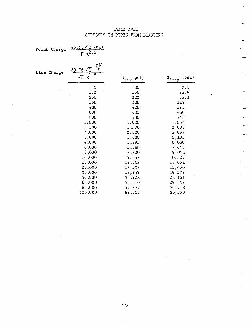
TABLE XVII STRESSES IN PIPES FROM BLASTING

Point Charge 46.53 IE (ftW) lh R2.5

nW

Line Charge 69.76 IE t /h Rl.S cr . (psi) cr

1 (psi)

cJ.r On!:\

100 100 2.5 150 150 23.9 200 200 53.1 300 300 129 400 400 225 600 600 460 800 800 743

1,000 1,000 1,064 1,500 1,500 2,003 2,000 2,000 3,097 3,000 3,000 5,103 4,000 3,993 6,036 6,000 5,888 7,648 8,000 7,700 9,048

10,000 9,447 10,307 15,000 13,603 13,061 ,•

20,000 17,537 15,450 30,000 24,949 19,579 40,000 31,928 23,161 60,000 45,010 29,349 80,000 57,277 34.718

100,000 68,957 39,550

134

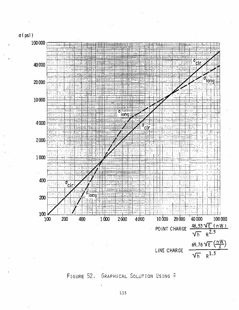
a ( psi )

100 ooo. i-----+-----+---+!-

POINT CHARGE

LINE CHARGE

FIGURE 52. GRAPHICAL SoLuTION UsiNG cr

135

40 000 100 000 46.53VE(nWl Vh R2.5

69.76 -VE (.IJf) Vh Rl.S

exactly on either the longitudinal stress o or circumferential stress long

lines in Figure 52.

As in the example used throughout previous discussions, a 40-lb charge

of AN-FO is placed 32 ft from a steel pipe 0.5-in. thick. Using Equation

(91) for a point source to compute cr gives:

cr = 46.53 ~9.5Xl0+6 (40)

Yb--::-s-( 32) 2 . 5 = 2468. psi (102)

.. Now we enter Figure 52 for a o of 2468 and read off of the ordinate that the circumferential stress

o1 equals 4200 psi. ong

cr • equals 2450 psi, and the longitudinal stress c~r

These answers differ slightly from the actual ones

be·cause of the accuracy which may be obtained from such a graph.

Most of the advantages and disadvantages remain the same as in the pre­

vious presentation. Probably the one added advantage is that no extrapola­

tion procedure needs to be learned to use Figure 52. Both axes in Figure

52 are, of necessity, log axes. Some engineers in the field might have

difficulty in using this type of graph paper.

Solution by Nomograph

The previous solutions all required that some computation be done before

obtaining the blasting stresses from a graph, table, or computation. It is

possible to present a nomograph with all the parameters shown separately.

Figures 53 and 54 are these nomographs for point and line explosive sources

respectively. One begins in these nomographs by finding the modulus of

elasticity for pipe material on the vertical line. A horizontal line is

then run from this modulus over to the appropriate pipe thickness in the

contours in the lower left of the figures. From the pipe thickness, a verti­

cal line is run up to the appropriate equivalent energy release (lbs. of

AN-FO) in the contours in the upper left of these figures. From the energy

release, a horizontal line is run over to the appropriate standoff distance

in the contours in the upper right of the figures. Finally the circumferen­

tial stress from blasting and the longitudinal stress are read by dropping

a vertical line from the standoff distance to intersect the circumferential

stress and longitudinal stress axes.

136

'·

..

11))) 2!m «lXl 71))) !01))) EQUIVALENT ENERGY RELEASE nW f lbs ANFO l STANDOFF 0 !STANCE 200

Rifll 140 100 70

700

200

100

10

40

20

10

4

2

0.1

0.4

0.2

0.1

32

14

10

5.5

4

3.2

2.5

2

I 1hL 1 qmu!uuuudtw!unbnd !I ddt! 1 ! J! !!!t!luutqhwftw!!mp I d! I!! 1 1 1 I ptpl"mlflrll! !!"!l.!Ufd 1 I

100 200 om tl)l) 2!mi .mo 101))) 20000 40000

I CIRCUt.'fl!RENTIAL STRESS acir I Jl$1!

2 luwn'W'M*+''II!!MuuqwluuluJqeltwl 1 I 1 f tit! 1 1, t 1,11 d!ll!!lwf 1,, d

100 200 om 1000 .mo fm! 10 ooo 201))) 4001:1

4 LONGinJOINAL STRESS 11!ong ( Jl$1 l

10"

4

6

1lf TABLE OF EQUIVALENT ENERGY RELEASES EXPlOSIVE _n_

Pt:NTOliTE I 50150 I TNT ROX __ ...,_ _____ .,.._ .,.-.

COMP B I 60140 I HBX-1

1.11 0.98 1.16 1.12 0.83 1.00 I. 05 1.12 0.99

1110 114112 I 2 PIP£ THICI<N£SS htinl

.wlDUlUS Of

ELASTICITY

AN-FO ( 9416) NG DYNAMITE I 40'- I NG DYNAMITE I 60'11 I AN lCNI DENSITY DYNAMITE

FIGURE 53. PIPE STRESS NoMOGRAPH FOR PoiNT SouRcEs

137

0. 7

0.4

0. 2

0. I

0.07

0.04

0.01

0.01

0.001

0.004

0.002

0.001

0. 0007

0. 0004

7 10 20

1110 !14 112 I 1

ENERGY RELEASE nW ( lbl ANfO) * 40 PER UNIT lENGTH OF liNE T II

3/16 318 314 312

PI Pt: THICKNESS hi 1n I

I 1, 11 11 , 11 :~mwudl!ll'!!"hV.C", "!.',,, l!!l"!:."*!l"whm'""'' 1 '"'", , , 11 " ll'"w"ll' I! !!I"!!""','

100 200 400 100l 2000 j 4000 IOOOl 2000l <llOOl I CIRCUMm!EHTIAt S'mESS ocir 1 psi 1

6

Jo"~'l

4 MJOULUS

Of 'IASTitiTY

!"'"'U .. MPWd,!•btlu!!"";''ll'hwt .. !"'!, !,l,J,!,,, ''''''''Ill!"!!''''''

100 200 «Xl lOOl 4000 6COl !OOOl 2000l <llOOl LONGITUDINAl S'mESS o!onq l psi I

*Total weight of explosive divided by total length of line.

TABU: OF EOU I VAlENT ENERGY RELEASES EXPlOSIVE ...!!._

PENTOLITE I 50150 I TNT RDX COMP & I 601<1!1 H&X·l AN·fO 194161 NG DYNAMITE I <ll'lo I NG DYNAMITE I 60'1o I AN li;WI DENSITY DENSITY

1.11 0.98 Ll6 1.12 0.83 1.00 1.05 1.12 0.99

FIGURE 54, PrPE STREss NoMOGRAPH FOR LINE SouRcEs 138

..

Both nomographs represent graphical solutions to Equations (91), (95a),

and (95b). Basically, logarithms are being added and subtracted until the

quantity a is computed. For a point source, Figure (53) is using Equation

(91) in the form:

[log a] 1 1 ' 5 = 2[log E] - 2[log h] + [log n.W] - 2[log R] + [log 46.53] (103)

The vertical line which finally descends to intersect the two stress axes

is the [log cr]. Both of the stress axes are not log scales because Equations

(95a) and (95b) are not log linear. But in both of these equations a . and c1.r al are unique functions of only cr. ong This observation means that a stress

axis can be computed from equations, and drawn from Equations (95a) and (95b).

Although portions of this line may be approximated by log scales, all seg­

ments of this line will not maintain the same proportions.

The same illustrative example of a 40-lb charge of AN-FO placed 32ft

from a steel pipe 0.5-in. thick is presented in the point source solution,

Figure 53. From this figure, one would estimate the circumferential stress

as 2450 psi and the longitudinal stress as 4050 psi. Once again graphical

accuracy prevents the solution from having the precision of an answer obtained

by substituting into equations.

The illustrative example presented in the line source nomograph,

Figure 54, is for a steel pipe, 0.5 in. thick, with 8 AN-FO explosive

charges weighing 0.5 lb each spaced 5.0 ft apart in a line 7 ft from a

pipeline which is parallel to the explosive line. The quantity nW/i

equals 8(0.5)/8(5.0) or 0.1 lb/ft. In this example, the circumferential

stress is 2800 psi, and the longitudinal stress equals 4850 psi.

Both of these nomographs have the added advantage that they can easily

be solved for limiting values of other parameters if a maximum stress is

specified. For example, suppose that the longitudinal stress from blasting

had to be limited to 4050 psi for a steel pipe 0.5 in. thick which had been

buried in the ground. The crews in the field might wish to know which com­

binations of explosive charge \veight and standoff distances constituted an

acceptable threshold. In this case, a vertical line would be drawn from the

4050 longitudinal stress axis on the right hand side of Figure 53 if point

sources were to be used. The same horizontal line would be drawn from E to

139

h, and a vertical line would also be drawn from h on the left hand side of

Figure 53. Now the correct answer relating acceptable values of nW to R

would be all horizontal lines intersecting the vertical lines on the left and

the right of Figure 53. The horizontal line which is drawn connecting an ruW

of 40 lb to an R of 32 ft is but one answer. For a 20-lb charge, an R of

25 ft is acceptable; for a 2-lb charge, an R of 10 ft is acceptable; et­

cetera.

The great advantage of these nomographs is their simplicity once they

are learned. No multiplications of powers have.to be taken to read stresses

or other quantities di~ectly. Their weaknesses are that their use must be

learned, inaccuracy can result if' lines are not drawn carefully, and field

personnel still have to read a graph which looks somewhat like. a log scale.

These nomographs have been drawn on a sheet of paper. Another presentation

which might be more attractive in the field would be to make a linear or a cir­

cular slide rule for performing these same computations.

Tables for Various Pipe

This format could be applied for a particular company application. A

field manual could be created in which all possible conditions had already

been precalculated. The following four pages are such a table for a point

source charge against a steel pipe which is 0.5-in. thick. This pipe may be

of any diameter; however, as soon as a line source is used instead of a point

source, a PVC pipe is used instead of a steel one, or if a pipe with a wall

thickness other than 0.5-in. is used, four more pages of tables would be re­

quired. Listed in Table XVIII are circumferential stress (SC) and longitudi­

nal stress (SL) for various equivalent charge weights (nW) in pounds of AN-FO

and standoff distances (R). Use is very simple provided the conditions needed

are included in the compilation.

For our example problem of 40-lb of AN-FO located 32 ft from a 0.5-in.

steel pipe, the tables which we have compiled can be used provided the read­

er extrapolates. The following four conditions shown below can be found in

Table XVIII.

140

TABLE XVIII

~iREj~ lrl 8URIED PIPE FROM POINT SOURCE BLASTING

1. t101~H3~~1E+C1(1 1. (1(H)(H)EH30 1, (H~H30t1E +0~3 1. (1(1[H](1E+OO 1. oo~:11~n~1E+0o 1 • (HZH] ~3 ~~1 E + (H]

1. 0(H3r!h::)E +00 1. O~J~::n:10E H](1 1. (H]00~3E+00 1. ~Z10~~H)(1EH30 i. (HJCH::H~E+(10 1. o~:::100~~1E+O~J 1 • (H~H) ~~H) E + (H]

1. 00~30~~1E+0~:::1 1. (1(H](1[1E H~H) 1. ooo~~n3E+tH3 i. (1(H](1~2IE+OO i. ~~H]~)I~H?,iE +00 1 • ~::HJ ~::HJ (1 E H) (1

1, ~~H~10(H~1E +00 1, 0CH30(1E+fH~ 1. 00(1~30EH~H3

2:. 0(H3[H3E+OO 2. (1l.h3~3~3E +~30 2. ~ZH3~Zi0~3E +0~) 2. ~3 (HJ(10E H) I) 2. ~)(10(10E+(I(1 2. ~)(H3t::10E +~'3~J 2, 0~JI2tt'30E +00 2. 0[HJ00E+CH3 2. Ot10{:)1~1E +0(:1 2. (H)(i(H3E+(H] 2 • fH:n3 ~::HJ E HJ (1 2. 00~JO~JE+~:.10 2, (H)(1(10 ~)[I

2. 0~::1(H30E +[H) 2 • (H~10 (HJ E HH~1 2, ~](1000E +0~~1 2. ~3000~JE H~n:1 2. ~J>JO~:n3EH)0 2' 000[1(1 (1~~1 2. 00~~H](1E+(H) 2. (H](H)~~1E +00 2. ~30~J(H)E+0~;:1

5. ~:::10(100E+~J~J ::i. o~:100~~1 t~0 5 , 0 C1 ~::1 ~71 0 E + 0 0 '5, OC,~:-iiJOE·+-;:)~.:1 c; , ~J >:.1 t i 11 ~:.1

f;.: < FT>

2.6::::7 E+~31 2.:31:2?1E+01 2. ~Z12758E+(11 1. ???60[~+0 1 1. 55:344E+O 1 1. ::::6630E·+·O 1 1. 1'3?B5E+fH 1,[150l?EH~11 9' 20 6')6[ tl21~21 :::. [1?1:::sE+00 ? . ~3?66:::E+121121 6. 2C1421E+12t0 5. 4:3 9:3~JE +00 4. ?6:::69E+0~:1 4.1:::[f??E+~:::10 :3 • :s ::;: 3 E + 0 (:) :::, 21 ::::4:3E+iJI21 2.:31 ?25E+121(D 2. 46 ·::~·;.t2E+·I210 2. 16:54[1[+~30 1. :::9:::4:3E+UO 1. 664J:::E+[H)

3. 4:::07?[+1211. 3.05163E+t31 2. 6754~~1[+(i:i. 2.34555E+Ol 2. 0563?E +121 J. 11l ::aZ1;2:35t:::+l211 1 , 5 ::: 1J 5 :::: 1:: + (11. 1. :::::::57J.E+·01 1.214:::7r~+ot 1. ~365~39E+O 1 ·:;t. :~:::::?7.:~E+O(t ::: • 1 ::: r.:: 5 (1 E + [I ~:1 7. 177201:-:+[11] 6. 2'3:233[+(~10 5. 51656E+Iali:l 4. ::::~:64:~:E+(t1;:1 4. 24 ~:115E +00 :3.71 ?:39E+OO ::::. 25'3!07E:+cn:'l 2" :;::5'?27E+I~il;;) 2 • 5 0 5 [H;.1 E +· ()1:~1 2.1'3616[+00

5. (12171E+(I:l 4. 40259t=:+IJ 1 :::: ~ !:: 5 '31 ::: ~~ E + 1211 :~: ~ :~: :::::: '3 :~: E +(t 1 2 .. 9667JE+~3l

:;:;C( I)

1, (100~~1f::IE+CI2 1. 3:::·;:;t50EH];2 :t. 9J~~1? :l E+·0:2 2. 6:::272E+(12 :3. ?2'?64E+02 5.:1.7956[+02 ? • 196'39E H12 :l. 001)(1;2[ .. 1-03 1.,J :~:1::1-~)J

1. 9:312175E+03 :2. ::;:1?.15[:.+ (1:::: :] • 6 ::! ~::.~ 1::: + ~z1 :3 ~i. l~~~~;::~~E+~)J 1:: n 9!::: :l5:::E + 0:~: ').4471'?E+03 :1.. :27069E+04 1. ~1:3::::E+04 :~~. 265::::2E+1~14 ::::: .. 00634E+f34 :3" 9 '? 6 2 ::::E ·1 .. f14 ;5R 24:34~:5E+~:::1.:.} 6 • :::: '316 HH.:: H] 4

1 " I~H.::II) (H3 E H12 1. :::::::::950E+~32 1. 930? :l E+l212 ~:~II 6:~:;2?;2[·+·~32 :::::. ?2:?64E·+·~]2 ~:3. 17 6E·t .. ~32 ? . l96'::.t9E ·+· 02 l. f3CIOO::~E +~:1:::: 1 • :3 ::: '31 5 :::: E ·+· ~] :~: l. 9::::0?~5[+~.::13 ;2 II 6 ::: :~:: ~~~ 5 E ., .. tl :~; :::II ?26:39E +~jJ 5.1:22:::4E+~J:~: 6 • ~::~~ ::: l 5 :::: [ ··t- ~J :::: 9. ·'+4? 1"?E+ 1 ':27[16'~4 1::+£14 1.. ?~?:1(13::::[+1~14 2. 265:3 ·+·e4 ::::. 0(~16:::::4[+04 3. ';t?62::::::E+~:14 ~) ' 3 ·+ ~:) [ + 04 6. :::961 OE ·r- (14

1. 00121~~~01:::+02 1. • ::::::::: '31 ~51:)[+ 02 :[ • ') J ~~I (' 1 [ + (1 ~=: ;;::: w ~~; ::: 2 7 2 E + 0 ::~: II ? ~:~ ? 6 4 E ·+· ~3 2

141

2. 51254E+(H~1 1. 84717E+t11 4.B6711?.1E+(11 1. 02'~55E +02 1, 9 £14E +(12 ::::. 57461 E +(12 6.2461'3E+ 1. (164:36E H33 1. 7:::[16(1E HZ13 2. 93741EH:13 4 • 7 :;:: ~H ::: E + 0 :::: 5. ?'326~~1E H33 ? . 0 1945E +0:::: :::. 50614E +(1::=.: 1 , ~3Jt177E +(14 1. 249~]::;:[+>~14 1. 5136::::E+t14 1. ::::::421 E H34 2. 269E+(14 2. IS'31:34~3 E +,~14 3, 26::::91 E +04 :;: ' 9551•:)E HZ14

2. 51254EHH3 1. ::;:4717EH~11 4' :::67 H1E H~11 1, 02955E +0:2 1, '37J04EHJ2 3.57461E+C12 6.24619E+~Z12 1. f"%4:36E+0:3 l. 7:::060E+O:::: 2. 9::::741E+(I:3 4. 7::H~1:3E+ 5. ?'3260E H~1:3 7. ~31945E Hr:: :::. s~?t614E+o:::: 1,[1::::~:17?EH.H

1. 2·::J.9(1:3E+04 1,51J63E+04 1 , ::: :3 4 2 1 E + 0 4 2.22269E+04 2 It 69345 ~~14 ::::. 26:391 E +04 3. 95~519E +[14

2. 512:i4EH.W 1 • ::::4 71 7E +01 4, ~::671 OE H::11 1. C129:55E·H~I;~~ 1 .. ·::.~ ~ :3 [14 E +· ~1 ?

5. (;O~~;(;OE +~)0 5. ooo~:;£;EHHJ 5 • (H) (H) [1 E HZH) 5. ~:n:nJt10E H)0 5. (t(1(H~H3E+0~) 5. 00~:n:u~1E+0~) 5. 0~30~:uJEH30 5 • ~::m 0 E:n:; E + ~~n:; 5. 0(H30~3EHJ~:; 5. [1(H](HJE+0~3 5. ~3~3(H)(1E H)(; 5. ~3~J~:;£;0E+~3~3 5 • 0 ~J ~:H:n::; E + (n) 5. ~3~:1tH30EHH3 5. o~:u)~)~JE H)(i 5. 0£n:;(uJEH30 5. 00(H)(iEH3~:1

1. ~3~3~30~3E+O 1 1 • ~:u:u:n:3 0 E + (11 1. ~::H:100~)EH31 1. 0~3~300E+£11 1. ~:n3~3~3~:;E +D 1 1 > ~3 (h) ~:H3 E H:1 1 1. CH)0~:u3E+01 1. ~:1t1000E +01 1.(H)(i(H)EH)1 1. (H~U)~)~:;E+01 1 • 0 (H:HJ ~) E H:1l 1. 00tn:H3E+01 1. [1(Hj(HZ1E +0 1 1 • ~:nJ 0 (1 0 E H:1l 1. ~J(H300E H) 1 1. (1(1[H)(1E+(11 1. 0~3~3~H:1E+~:11 1. ~3~3[1(H)E+01 1. (1tH:H::HJE +(11 1 • 0 ~:u:; tH3 E Hill 1. ~3~J~:::H:nz;E+(11 1. 0(Hj~J~)E+01

2. ~::H30~:1(1E H31 2. 00[HJ~:iEH31 2. (H:i(H30EHH 2. (1(H)0(1E +0 1 2 • ~:10 ~:nJ (! E H:11 2. ~J000~3E+01 2. (;~:1~:;0~~1E+[11 2 • 1:10 ~~a:u:; E + (11 2. f;0~300E +01 2. (HJ00(1EH:::11 2 • (1 (H) (n:; E H~11 2. 0~30~3~3E +01 2. (1Cn:1(10E +01 2. 1)(10~:;~:1E+~J1 2. 0(H)(u:;E + 01 2. (1(1(1(H3E+(11 ,::, u~:::o.j~:.;c · •.t:. 2- 01~10lj!j[ :.~i i

2. 6~:nJ•??EHH 2. 2::: 03~3E +0 1 1. 9'3916E+131 1.75269E+01 1. 5366~3EHH 1.34716EH~11 1. H: H17E+E11 1. ~3:3545E+fH 9. 07794E+~]I~ 7. 95:373EHH.::t 6. '?7751EHJ0 6.11726E+€H] 5. :~:6:::::f17E+00 4. 7~3 1 ::: 7E -H::H~1 4.1221:3E+€H':.1 3. 61396EHH3 :~:.1684~31::+00

6.62619E+01 5.:30925E+01 5. (19:304EH~11 4. 46512E+t11 :::;: • '? 1462EHH 3. 4:~:2[1(1EH31 ::::. m:::t::::::7E+01 2. 6:::::791 EHH 2. 3126:3EH31 2.02756£+01 1' 7775:::1::+01 1. 55:::4:~:E·H11 1. 36629EH~1l. 1. 1'37S4E+01 1. ~:15016E+t1l 9. 2t16::::::E Hh~! S. ~371 7SE +€10 7. 07662EH30 6. 2~~1415E+0[1 5. 43925EH30 4. 76:::t::5EH](; 4 • 1 ::a3 7:~: E H3 ~.:.'!

S. 74331E+~Z1l 7. 66536E+fZ11 6. 72t131E+01 5. B';.t 177E+[11 5.16 :::E+Ol 4. 52:::s5E+~:n 3. 97023E+~31 :;: • 4::: t174E HH :::;:, 05161EHH 2. 675:~::::E+(11 2.34553E+01 2. (15636E +C11 1 . ::a3 2:::3E H:11 1. 5C:0:i6E+Ol 1. 3:;:570E+O 1 1. 214::::6E+~H 1. ~365~]:::E+€11 '}. 33?f:5E+[1~)

142

5. 17956E+€12 7. 196'?9E+02 1 • ~.:.h:u3 ~~~ :2 E + 0 :3 1. :3:::·~53E·+-0-:3 1. 93~~75E+03 2. 6::::3~~15 E + o:~: :;: • 726::::9E + E1:~: 5.122:::~tE+~J:~: 6. ·~::: 1 ~s;::E -1- ~3:3

9.4471?E+03 1. 27069E+t14 t •. ?t1~:::t:::::::E+~34 2. 265:32E + ~34 :~:. [I~ZI6:~:4E ·H:::t4 :;: • '3 762:::E + (14 5 • 2 4 :~: ·4'5 E HZ14 6. :396H1E+~34

1. [H]0~]CtE+~32 1. :~::::9~5~JE+€12 1. 9::H~171 E + €12 2~~ 6:::~~72E+~32 :3. 72764E + 02 5. 17956E+€12 7. 196~~9E+~~12 1, (10C102E+~Z1:3 1 ~~ :3::: E+~~13 1. 075EH:t:3 2. 6 05E+(13 ::;:. ?~::~s:::9E+€1:3 5.122:::4E+~]:~: 6. ~:,t:;::t:i:::E+£1:3 ·:;t. 44? 17E+(1:3 1.2?069E+04 1 • 7 ~H] :?:: :::: E ·+· 0 4 2. 265:~:2E·+04 :~:. t10634E +(14 :3 • *3 ? 6 2 ~:: [~ + ~3 4 !:i. 2434~5EHH 6. ::::'36 HiE H)4

1. OI210~7:1~3E+~Z12 1. :3:::·350E+02 1 • 9 :::n~f? 1 E ·H~i :2 c~. 6:::~~~:?2E+02 ~3. '?2 ?1:~4E + (12 5. 1 ?·::~st::l::+€12 7.19699E+02 1. f3tH~H32EH:13 1 • :~: ::: ';:!i 5 :3 E ., .. ~~1 :~: 1. 930?'5E+~3:::: 2. t.:=.:::::::05E+t13 :3. 726::::':~E+(1:~: ::5 II 1 2 ;~:~ :::: 4 E + (1 :~: 6. lt:5::::E+O:::: '3 • 4 4? 1 ? E + 0 :::: 1. ~=:?Ot:~·:::•E+~34 1. 7(W H34 ~-:_:. 26 2E+04

:3. 5!'46 1 E +02 6. 24619E+'J2 1. ~36436EHn 1. 7:::(16t1EHZ13 2. '3:;:741E+~Z1:::: 4. 7::a:::11 :::E +0:~: 5. 7926(1E+0:3 7. (11 '345E+t1:3 :::. 50614E+t1:3 1. ~33~377EH)4 1. 249E1:3E+04 1. 51:363E+04 1. ::::3421E+f14 2. 22269E +~Z14 2. 69:345E+t14 ::::. 26:3'31 E +~34 ::::.95519E+04

2. 51254EH3~3 1. :::4717EH31 4. :::67 H1E +t11 1. D2955EH32 1.97304E+02 J. 57461EH32 6.24619E+02 1, ~::164:36E·H~;:3 1. 7:::060EH):3 2. '?:3741 EHB 4. 7:::~31f:E+0:3 5. 79260E H~;:::: 7. [11945E+t13 :::. 5~~1614E +(1:::: 1. cno77E+t14 1. 24908E+(14 1. 5136:3E+D4 1. ::::~:421 E H)4 2. 22269E +(14 2.69:345E+04 3. 26:3'? 1 E +04 :3. 95519EH34

2.51254 ~]~) 1. ::::4717E+Ol 4. :::67 U3E +01 1. (12955E +02 1. '?7:304E+C12 :3. 57461E+l12 6.24619E+02 1.064:36E+0:3 1 .7::.: [16~~; E + t)3 2. ·?::::741 E +tn 4 • 7' ::H.::11 :3 E H.r::: 5. 7')260E +0:::: 7. C11':;;45E H~;:::: ::: • 5 ~J 6 l 4 E + 0 :3 1. 03~J77EHH 1 • :~: 4 '3 0 ::: E + t14 1, 51363E +~:j4 1 • ::: :;: 4 :,~ 1 E: + 1~14

2. t1 o~:::1~J~Z1E ·i-(11

2. 0(10t~HJE +0 1 2, ~30~)00EH~11 2. t1(H;.H)(1E +01

5, 0tH)(1~)E H) 1 5, (1(1(H)0E +~) 1 s·. 0£1(HZ10E HZ11 5 • ~] ~)(1 (H) E H~11 5, ~ZHZ1 00~:1E H) 1 s . ~~1 £n) ~::wE + ~:::11 5. ~Jm3~~H3E+t11 5. 0[H)00EHH 5. (1(10~:10EH31 5. (I(H)(H)E H] 1 5. 0(H)00E+01 5. (1(H)0(1E+~) 1 5. 0[1(HZH)EH) 1 5. ~Z1t10(n)E+01 5. ~)fH300E HH

. ''''5 ..• 000(1(1E+(i 1 5 :·t~HJ00~~1E+01 5. ~)[H)(H)E +~] 1 5. 0~J[H)~)E+(11 5. 0~~B)fj(1E+01 5. [1(H300E+(11 5. ~)(1(H)~]EH) 1

1. ~)0~ZH3t1EH32 1. (1(1(H30E+02 1. ~)[H3mJEH)2 1. (1[H)(H3EHJ2 1. 0~Z1(H)~Z1E+02 1. ~)~J~:::nJ(1EH~12 1 • ~:::10 ~3 0 ~~1 E H:12 1. (H)~)~)t1E+02 1. (1(U)0~Z1E+t12 1. 0~Z1(HJ0E+02 1 • fHZnJ ~) ~:::1 E H::12 1. o~:1oo~:::tE+o2 1. (H)~J~30EHJ2 1. 01ZH3~J~JE+02 1. (H3000EH:12 1. 00(H30E H:::12 1. 000~:::10E+~32 1. (10(H)~]E+t12 1. ~3~:1(H30E+t12 1. 000~)(1E H:::12 1 • ~ZH~h:H) (1 E H:::12 1. (H)(HJ(1E+02

2. (1(n:::nJ(1E+~32 2. ~300£H.::1E+02 2. ~)(H=H~10EHJ2 2. 00[H3f1E+02 2. 0(n:nJ~:::1E HZ12 2. ~:::1(1 OO~JE +(1 ~: 2. ~J~:.HJOOE H:::12 :::: • 0 0 ~J 0 0 E + 0 2

8.1:3642E+(H~1 7.17713EHX1 6. 2'3227E+£1(1 5. 5165t1E+(H]

1. 26 14~3E +(12 1. HJ5::::::EHZ12 9. 69538E+£1l :::. 5~3~3~~15E+01 7. 452(19E+I2t1 6 • 5 :3 :~: :::: :3 E + ~z1 1 5. 727:::5E+t11 5. ~~12167EH:::11 4. *~1255EH:11 :~:· • ::: 5 ·~ 7 7 E + 1~1 1 :3. ::::::: :3'3~Z1 E +01 2. 9667t1EHH 2. 60~:::194E+~:11 2. 2:3~J2:3E+01. 1. '3'3914E+~11 1. 75267EH3 1 1. 53659E +(t1 1.34714EH)1 1. 1:::1 06EH3 1 1. ~):35441::HJ1 9.~17 6E+~~HJ 7. '35S66E+1211~1

1. 66442E-H:12 1. 45922E+~~12 1 • 2 7 ';J :3 1 E + t12 1. 1215'3E+~Z12 '3. :3:3309E+~1l :::. 62 ~)7:::E +(11 7. 55794E·H11 6. 626t:;:EHZ11 5. ::;:(1':.42~:1E H) 1 5. ~39299E+[1J. 4. 465~~t:3E+01 ::::. 91459E H:11 3.431'316E+01 :;:, 0(1::::::4E+O:l 2. 6:37:::9EHZ11 2. :~: 1266E+~31 2~02754E+01 1. 77757EHH 1. 55:::41 E+f) 1 1. :3662SE+01 1. 197:::3EH31 1.~35015EHJ1

2. 1 '3622E+~~12 1. '32545EH:12 1. 6~::::(16E+02 1. 47'395EH:12 1. 2974:::E+~:1~: 1. 1:3752EH~12 9. 97276E +~) 1 :::. ?432::::E+O 1

143

:3. 0(16::::4E+~34 :3. •;.762~::E+~J4 5. 24:34~3E+04 6. :::9610E+04

1. ~30(100E+02 1. :;::::950E+~::12 1, '3:3(17 :l E H32 2. 68272E+~32 :3. ?2'?'64E+l12 5. 1 ?•;j56E H~12 7. 196':.•·~~EHJ2 1. f~112H3~32E+03 1. :~::;::95:3E+(1:~: 1. 9:3[175E+O:::: 2. 6::::::::~J5E+~:1:3 :3. 726:::·:~E+(1:3 5. 122:::4E + Et:3 r;;. 9~:::L5t~:E+~3:~: 9. 44717EH3:3 1. 2706'31EH34 1. ?0~J::::::E+~J4 2.26 2EHJ4 ::::. 12l~:t6:~:4E+~Z14 3. '3t'7~:~2::::E+~J4 5. 24:345EHJ4 f.::~. :;::·~~61 (1E + t14

1. 00\~H]~~IE+t2t2 1. :::::::·~50E+02 1. '3::::~Z17:lE+02 2. 6:::272E + (12 :::: ~ 72?64E+t12 5.:l7956E+02 7. :t·~•69':3EH32 1. 0[101~1,:;:E+03

1. 9:3075E -H:n ~~~ . t: ::: :~: [15 E ·+- ~3 :;: 3. 15:::9E H:::(3 5.12284E+0:3 6. ·~815:::E + ~z1:~: 9.4471?E+t1J 1.2?069E+04 1 , 7 0 ~~ ::;: :;:: E + 0 4 2. 2t~:5:::::21:>t-(i4 :3. ~;)0634f~··l-04 :3.9?6 E+~:14 5. 24:34~5E+t14 6. :;::·:;:~6 HJE+ 04

1. 0J)I2100E+02 1. :;::=::·~5~)E+t12 1. 9:::1::171 E+02 2. 6:::27:2E·+·t.]2 :3. 72?64E+t12 5. 1 ?·:~56E+02 7. 1 '3699EH~12 1. 1,}00\::1;::E+03

2. 2:2269E+~J4 2. 69345E H?.14 3. 26:391 E +04 :3. 95519E+04

2. 51254E H3~:1 1. :::4717EHH 4.:::671 ~3E+~31 1. ~~12'355E H32 1. 973t14E+f]2 ::::. 57461E+t12 6. 2461'~E +~32 1. ~Z164:36EH:1:~: 1 • 7 ::: ~:16 ~~~ E + en 2. ~;t:3741E+~Z1:~: 4. 7:::ot:::E+£1:3 5. 7926~:1E+(1:::: 7. ~:11945E·Hj:;: ::: • 5 ~J 6 1 4 E H] :::: 1. 0:3~J77E H]4 1. 9~3:3E+~~14 1. 51363E+C14 1.:::3421 EH:14 2. 2226·::4 E+~~14 2.69345E+04 :;:, 26391EH:14 :;: • '3551 '3EHH

2. 51 ;~54E HZHZ1 1.S4717EH]1 4. :367H1E+t]1 1. 12t2955E +02 1. 973~Z14E+~212 :;: , 57461 EH:12 6.24619E+(12 1 • (16 4 3 6 E + (1 :~: 1. 7:::o6~~1E+OJ 2. 9::3741 E +(1:~: 4. 7:::~~118E+(i:3 5. 7'326(1EH:J:;: 7. t11945E+0:3 :::. 5(1614E Hr;: 1. 03t177E+(14 1. 249t1:3E+C14 1 • 51 :36:3E +(14 1. :::3421 E H]4 2. 2226 13E+(1.:.1· 2. 69J45E+(14 ::;: • 26:391 E H34 3. 95519E+~34

2 •. 51254E+(n;:1 1. :::4717EH:11 4. :::671~3E+Ol 1. ~32955E H:12 1. '37:3t14EH:12 :3.57461 E+C12 6.24619E+02 1 • 0 6 4 :?: 6 E ·r \?! :::

2. ;)(il~i>3E1E+~J2 2. 0>3000E+02 2. 0000~3E H);2 2 I ~1(H;:h)(1E H)2 2. 000•3•3E+•:12 2 • (H) £n:nz1 E H) 2 2. ~30CB30E+•:12 2. ~::HJ•XH3E+02 2. ~)(H;H30EH32 2. •ZU:30(H)E+02 2~ ~)(n:10~3E+02 2. 0•30tn)E+•:12 2. [100•J0EH32 2. DOOD•Z1EH:12

5. •J•J•J•)f1E +02 5. ~::Wt1[10E+02 5. (H)•J(H)E+02 5 • >)0 (1t~H3 E H) 2 5. •::1[H)[1(1E H)~

. 5. Ot112H£HJE+02 5. •J[H300EH32 5~ 0000f1E+02 5. 0(10•:nJE+02 5. (1[1000E +02 5, >)[H)(10E H)2 5. 00(H;.h]E+02 5. 0>)00(1EH}2 5. >)0(HZHJE H::12 5. (H)(i(H)E +02 5. (1t1000E+t12 5, [H)~::HZH3E +02 5. (H)>)[1(1E H)2 5. >3[1000E +02 5. 0000(1EH32 5, 0(HZ100E +02 5. EHZH)(1[1E +02

1. •J0>:1[1(1E +03 1. (1(1(1(10EHJ:::;: 1. •Z1>:100>:1E +o:::: 1. [100>Z10E +>~13 1 • (1 ~::1 >J>:1•:1 E + 0 3 1. (10>3tH:1E+0:3 1. •JOOOOE +>::1::;: 1. >:)0(1>:10E+>:13 1. (1(1(100E+0:;: 1. >::100>:::1f1E +>:::13 1. 0>:::11210(1E+03 1. O>JOOOE +0:3 1. >30t100E+O:::: 1, 00•30(1E+(13 1. 0>:100>3E+O:~: 1. >)0000EH}:;: 1. >J•J(nJ•JE+03 1, OOOOOE+~J:::: 1. (100>::1>;)E+03 1. [10000E+O:;: 1. ~30(100E H;:1:::: 1. >3>:100f1E+03

7. 6652'3EH~11 6. 72>324E+[11 5. :::'3 1 71 E HH 5. 165:3:3EH~11 4. 52 :::5(1E H~11 :::: • '3 7 ~~11 '3 E + 0 1 :3. 48>~171E+01 3.0515:::E+01 2. 675:35EH]1 2.::N551E+01 2. [156:34EH~11 1. 8~3281EH~11 1. 5:3055EH)1 1 • :3 ::: 5 6 ::~ E + ~!11

~:. 16:::4'3EH32 2. 777:::5E+02 2. 4:35:37E+~32 2. 1:3~:i12E+~~;2 1. :::71:3SE+€12 1. 64110E+02 1. 4:3:::77E+~32 1. 261 3'31E H)2 1. 105:::7E+02 '3, 6'35:3[1E+01 :::. 4'39'37E+~~1l ? • 4.5202EH.11 6. 5:;:::::27E+~Z11 5. 7277~~E+~)l 5. ~J2162EHZ11 4. 4~~1251E+01 J . ::: 5 ~:;t 7 :3 E + ~] 1 3. :~:::::~::::?E+€11 2. 9666:3E+01 2.60>:1 E+01 2. 2:3~J26E+~3 1 1. '3991:3E+C11

4. H:0:::4EH~12 :~:. 665Jt~E+t12 3. 21 ::::49E +(12 2. :::17~:::t~1E+~]2 2 • 4 6 '3 '3 6 E + ~:12 2. 16544E+(12 1 • ::: ~3 ::: 4 7 E + [12 1.66441E+02 1.45921E+02 1.279:30E+02 1. 1215:::E +02 9. :;:::;:JOOEHJ1 :::. 62071E+01 7. 557::~7E+~31 6.62607E+01 5. :::(1915E+01 5. 0'3295E+01 4.46504E+01 3. 91455EH~11 3. 4:::: 1'3::::E +0 1 ::::. 0(1 :::::::1 E +a 1 2 • 6:3 7 8 6 E + [11

144

1. :~::::'~5:3E·+0:3 1. 9::.::~375E+·~]:3 2. 6:3:305E+0:::: :3. 726~:9E+~;):~: 5.122B4E+~J:~: 6. ~3::: 15:::E·+tt3 '). 44 71 7E+(1:3 1. 2?~ZH5':::<E+04 1 • 7 1~1 ~ZI :3 ::: E "I· >3 4 2. 265:~:2E + ~)4 :3. 0(1634E + 04 ::~. 9762::::E+04 5.:24345E+04 ,;:.;,::: 10E+(14

1. ~30~~~~3>3E+(12 1 • :~;::: '' 5 ~~1 E + (t2 1. ·~::::•:171EH:)2 2. 6S272E+€t2 :3. 72764E +02 5. 17956E+02 ? • 196'39E+02 1. ~)~~1~.:HJ2EH33 1. :3::: 4'5:3E+~):~: 1. ·3::::12175E+t1:3 2. E:~:::::::05E+~~1:3 :3. 726:::~3E +~]:3 ~5.12:~:::4E+0:3 r:~ It 9 ::: 1 5 :::: t:: + €1 :::: '3. 44'?' 17E+(13 1. 2?06'3EH34 1. '?(1~1:;::::E-H34 2. 26~5:~:2E+-~34 :;: • 0 t~H; :;: 4 E + (14 ::::.976 EH}4 5. 24::::4::5E+>34 6. :::·::16 H1E + 04

1. OO~J~:10E+(12 l~a :~::::95(tE+~3:2

1. -:.<::::(171E+02 2. 6:::272E+~12 :~:. ·7:;:~ ?64E + t12 5. 17956E H]2 7. 191::99E+(12 1. 00002E·H1:::: 1 • :~; :::·3 5 :;: E + 0:::: 1. 9:~:(1'{5[+0:3 2. t.:::::305E + ~3:3 :3. 72(3:::9E+~Z1:3 5.12~~::~4E+~]:~: r.:;. ~31;:~ 15SE + ~]3 9. 44'?1?EH~1:] 1. 27~36'3EH:::14 1. '?00:::::3E+04 2 .. 21:::s:3~::E ·+· ~]4 :3. 00 4E-:+(14 :;: • ~~ 7 6 2 ~:: E + ~) 4 5.24345E+04 6. :::::'361 OE + ~Z14

1. 7S~36(1E +>JJ 2 • 9 :;: ? 4 1 E + (1 :3 4. 7::a31:::E+~J:::: 5. 7'3260E+03 7,(11945EH)2: 8. 5>J614E +(13 1. 0:::a377E+04 1. 2490:::E+04 1, 51 :36:3E H)4 1. :3:3421 E H)4 2.22269E+04 2. 6'3:345E + 04 :3. 26:391 E +04 :3. 95519E+(14

2.51254E+[10 1. :34 71 7E +01 4.:36710EH31 1. (12955E H)2 1. 97:304EHJ2 :3.57461E+02 6.24619EH:12 1. 064:36E +0:3 1. 7:3>J60E +£1:.::: 2. 9::::741E+(1:3 4. 7:::(11 :::E + 0:::: 5. 7'3~::60E +03 7. >::.li '34'5E+£13 8, 50614EH;:13 1. 0:3~]77E+04 1. 249~Z1:::E+t14 1. 51 J6::::E H.H 1. ::::3421 E +(14 2.22269E+04 2. 6'3345E+04 :3. 26:3'511 E H)4 ::::. '3551 '3E HZ14

2. 51254EHJ~J 1.84717E+01 4. 86710EHH 1. 02'355E+l12 1.'37:304E+02 3. 57461E+~~12 6. 24619E+~J2 1. 06436E HZ13 1 I 7 ::: 0 6 >::1 E + >:1 :::: 2. 9:3741EHZ13 4 • 7 ::: 0 1 ::: E + ~J :~: 5. 7'326>)EH~13 7. 01 '345E H~n :3. 5~~1614EHZ13 1. >33077E HH 1. 24'30:::E+04 1. 51 :~:6:3E +04 1. ::;::3421EH}4 2. 2226'~E +[14 2. 6'3::::45E+t14 :3.26391EH:14 ::::. 9551 '3E +04

TABLE XIX. STRESSES USED IN EXTRAPOLATION

n·w R sc SL

20 34.8 1000 1064 20 30.5 1390 1781 50 33.8 2683 4780 50 29.7 3727 5793

Extrapolating first on standoff distance gives:

= 1390 - 1390 - 1000 1136 psi a = cir20 lb 34.8 - 30.5

(104a)

a 3727 - 3727 - 2683 (33.8 - 32.0) 3269 psi = = cir50 lb 33.8 - 29.7

(104b)

a 1781 - 1781 - 1064 ( 34 . 8 - 32 . 0) 1314 psi = = long20 lb 34.8- 30.5 (104c)

= 5793 - 5793 - 4780 (33.8- 32.0) 5348 psi a = long 50 lb 33.8 - 29.7

(104d)

And finally extrapolating on charge size gives:

a = -(3269 - 1136) (50 - 40) + 3269 = 2558 psi cir40 lb (50 - 20)

(105a)

a = -(5348 - 1314) (50 - 40) + 5348 = 4003 psi long40 lb (50 - 20)

(105b)

These answers are close but not exact because of the extrapolation pro­

cedure. The advantage is that error might be prevented because items have

been precalculated. The disadvantage is the extrapolations which are required.

This computation required a double extrapolation--the standoff distance, and

the charge size. A third extrapolation could be required if the appropriate

pipe thickness was not listed. In addition, the number of tables which could

be required rapidly becomes very bulky especially if many pipe sizes, pipe

materials, and line as well as point sources are to be considered.

145

Graphical Plot of Parameters

All of the information contained in the previous table, Table XVIII,can

be displayed in a single graph plotting either o . or o1

versus (nW) and R c~r ong

for constant values of h and E. A series of these figures would be required

for various values of h and E. Figure 55 is one of these figures drawn for

a modulus of elasticity E in the pipe of 29.5 X 106 psi and a pipe wall

thickness h of 0.5 in. The dashed lines in Figure 55 are for predictions

of longitudinal stress o1 , and the solid lines are for estimating cir-ong cumferential stress o . . The abscissa is the standoff distance R and the

c~r · various isoclines are for constant values of equivalent energy release nW.

No extrapolating is needed for the standoff distance R, and any extrapolation

on energy release nW can be eyed. These are the major advantages in using . this approach over the use of tables.

The example of a single 40=lb AN-FO charge located 32 ft from a 0.05-

in. thick steel pipe can be accomplished by directly reading Figure 55 after

judging where the 40-lb charge line should fall between the 20 and 50-lb

charge contours. From Figure 55, we would fjs timate that the longitudinal

stress o1 was approximately 4000 psi and the circumferential stress was ong approximately 2400 psi.

The major advantage to using Figure 55 is that no computations are re­

quired. Several disadvantages are that no one figure or table suffices. and

field people must know how to read a graph and log scales.

The entire family of figures has not been drawn because pipe sizes and

charge ranges can vary from company to company. In general if this approach

is used, a complete set would be required. The equations being used are

the ones used throughout this chapter, Equations (91) through (95b).

General

In creating a company field manual, any of these approaches can be used

to obtain essentially the same result. Notice that essentially the same

estimates of circumferential and longitudinal stresses from blasting were

obtained using all approaches because the same problem and equations were

being solved.

Perhaps greater difficulties will be encountered when decisions are made

as to how longitudinal and circumferential stresses from other environments

146

cr( psi I h • 0.5 in

40000

20000

10000

4000

2000

1000

400

200

LONGITUDINAL STRESS n W ( lb I ( Dashed lines I

R ( ft l

FIGURE 55. GRAPHICAL PLoT OF PoiNT SouRCE BLASTING PIPE STRESSES

147

are included. The solutions presented in this section give only those com­

ponents of stress which are obtained from blasting. In addition,stresses

from: 1) thermal expansion or contraction. 2) differential settlement of

the pipe, 3) weight of overburden, and 4) internal pipe pressurization all

add or subtract from the stresses caused by blasting. In addition, the

subject of safety factors has not been discussed in detail and must reflect I

state laws and company policy. These added points are mentioned once again

to emphasize that this solution for stresses from blasting near pipelines

is only a partial one. The overall state-of-s~ress depends upon many

factors, and to represent all in a field manual could be a very difficult

task.

148

VIII. ANALYSIS OF STRESS SOLUTION

Example Problem

The solution for pipe stress which has just been presented is idealized.

In reality problems are not point sources or line sources parallel to a

pipeline. A problem which is more typical of a realistic field problem

might be defined as follows:

1) A pipeline is 30-in.in diameter with a 0.250-in.wall thickness,

and a SMYS of 60,000 psi. This pipeline is operated at a stress

level of 50% of yield in the hoop direction.

2) Ammonium nitrate/fuel oil is to be used as an explosive in

a 20 ft by 50 ft rectangular grid. The grid is rotated 30

degrees to the pipeline so that the nearest corner is 50 ft

from the pipeline. The next corner which is 20 ft away is

61.5 ft from the pipeline. This charge configuration is

illustrated in Figure 56. The parameter consists of fourteen

30-lb charges spaced 10 ft apart. These charges are to be

detonated simultaneously. Four 50-lb charges lie within this

parameter and are to be detonated with a delayed fuze (assumed

to be 1.0 millisecond).

3) Soil conditions are unknown. Solve to see if this blasting will

endanger the pipe.

The point made by this discussion is that real problems never corres­

pond precisely with idealizations which are made for computational pur­

poses. Engineering judgment is almost always required. There is no one

answer to a problem such as this. Probably the best approach would be to

solve this problem several different ways and use the answers giving the

highest stresses.

One assumption might be to say all 620-lb of explosive detonates

simultaneously as if it were located at a point in the geometric center

of this array. Answers of the correct magnitude should result from this

type of approximation, and might infer that no problem, a serious problem,

or uncertainty exists as to the pipeline's safety for such a blasting operation.

By sketching out a problem such as this one, additional ideas also can

be generated. For example, a delay-fuzing sequence should not be run towards tl:e

pipeline. Lower stresses would certainly occur if the charge nearest the

149

pipeline were detonated first and all delays progressed away from the pipe.

Such a suggestion should automatically be company policy so shock waves

from different sources have less chance of "shocking up" to form a more

severe shock front at the pipeline.

This problem will not be solved because: 1) different quantitative

numbers enter any problems and 2) various engineering judgments can be

justified. Problems such as this one will.be encountered and have to be

faced by each individual pipeline company.

Solution Idealizations

Another reason for presenting the previous example was to emphasize

that solutions are idealizations. No solution is properly understood unless

the'se limitations are understood. Among the many limitations to these

stress solutions are:

1) The charge and the center-line of the pipe are at the same depths.

2) A line charge is a continuous line rather than a series of point

charges. A point source has no shape or finite size.

3) Any line source r-.1ns parallel to the pipeline.

4) The pipeline is straight without elbows or valves.

5) Wrapping, sand beds, and other potential shock isolation layers

between the pipe and the soil have no effect.

6) The solution gives only the elastic stress contributions from

blasting. No inelastic behavior is included in this solution.

7) Explosive sources always detonate instantly.

8) Reflections from the surface of the ground are insignificant.

9) No explosive energy (or at least a constant percentage of the

energy) goes into cratering, air blast, and other phenomena.

Sensitivity Analysis

One of the best ways to determine how a solution responds to a change

in some variable is to perform a sensitivity analysis. The variables which

determine the circumferential stress acir and the longitudinal stress along

from blasting are the modulus of elasticity for the pipe E, the charge size

nW, the pipe wall thickness h, and the standoff distance R. For a line

source, the energy release n~ for a point source is replaced by an energy

150

• • •

• • •

• • • 50'

• • •

• • •

/L:o.j """"

f 50' .....

'

• 30 lb Charge

I • 50 lb Charge 30 in.

FIGURE 56. PLAN VIEW OF AN EXAMPLE FIELD BLASTING PROBLEM

151

n"W release per unit length ~· Although the influence of E and h remain the

same in both point and line source solutions, the standoff distance Rand

the energy releases nW for a point source and ~ for a line source have

different influences on pipe stresses for point and line sources.

The solutions which have been developed can be seen in Figure 52.

Whereas the circumferential stress solution is almost a straight line in

Figure 52, the longitudinal stress solution has a sharp break at 2675 psi.

This observation means that the influence of the various parameters E, h,

nW, and R on stress· differ for longitudinal stresses dependent upon o being·

larger or smaller than 2675 psi. Probably this break is caused by the pipe

responding in different modes. This influence on circumferential stresses

is .not great enough for a separate circumferential stress evaluation.

Table XX presents the results of a sensitivity analysis. In this table

each parameter E, n"W, h, and R are doubled independently. The number in

the table shows how much o . and o1

increase or decrease because the c~r ong

parameter was double. If the number is greater than 1.0 as for E and n"W,

the stress increases. If the number is less than 1.0 as for h and R, the

stress decreases. Two rows are used to present o1 results, and are ong dependent upon o being less than or greater than 2675 psi.

TABLE XX

Results of Sensitivity Analysis

Stress PiEe ProEerties Point Sources Line Sources n"W Com:eonent E h nW R £ R

o cir 1.41 0.71 2.00 0.18 2.00 0.35

o long large 1. 22 0.82 1.50 0.37 1.50 0.55

o long small 1. 75 0.57 3.08 0.06 3.08 0.19

Table XX indicates that stresses are most sensitive to standoff distance

R and least sensitive to the pipe properties E and h. Changes in the stand­

off distance also have a greater influence on point than line sources.

The list of parameters in Table XX, may seem small; however, these

parameters are the main ones which determine the change in stress in a buried

pipe from blasting. Particularly obvious by their omission are the pipe

152

diameter, the soil density, and the seismic propagation velocity in the soil.

These parameters are absent because the solution is independent to them.

In the case of larger diameter pipes, more kinetic energy is imparted to

the pipe as its diameter increases, but more strain energy can also be

stored in pipes with larger diameters. Because of the increase in kinetic

energy and strain energy, both are increased by the first power of the

pipe diameter. The pipe diameters cancel when these quantities are equated,

and the resulting response becomes independent of pipe diameter. Experi­

mental tests on 3-, 6-, 16~, 24- and 30-in pipe all yield results that show

this observation is a correct one. X p 1/2

In a similar manner, the approximation that R (~2 ) is proportional

to ( ~ 3) eventually leads to p and c falling out o~cthe analysis. If the

morePEo~plex hyperbolic tangent relationship is used, the circumferential

stress and the longitudinal stress become weak functions of p and c. The

simpler format was used, because adequate engineering answers were obtained

without appreciable benefit from added complexity.

Other Stress States

A knowledge of the state of stress caused by blasting is necessary but

not sufficient information to determine if a buried pipe will yield. Other

loading mechanisms also cause a pipe to be stressed. Because of symmetry,

circumferential and longitudinal stresses from blasting and other effects

are principle stresses. This observation means that an accurate estimate of

the elastic state of stress can be made by superposition through addition of

stresses with their signs considered. The purpose of this program does not

include a discussion of states of stress ~from other causes. These stresses

can be very significant, so readers should consider including longitudinal

and circumferential stresses from such causes as:

1) Internal pipe pressurization

2) Thermal expansion or contraction

3) Surcharge or overburden

4) Residual stresses from welding and

other assembly processes

After the resultant longitudinal and circumferential stresses have been

obtained, a failure theory will have to be selected to determine if the pipe

153

yields. In this discussion we will only mention some of the theories which

might be chosen. Actual selection of an appropriate failure theory must be

left up to engineers in each company. Sometimes state law, politics, and

other considerations beyond our control dictate the choice or selection of

a particular process for determining yield. We will illustrate some of the

theories which might be selected.

A biaxial state of stress may be plotted on a graph with one stress

such as the circumferential one on the X axis and the other such as the

longitudinal one on the Y axis. Figure 57 is such a plot, with the circum­

ferential and longitudinal stresses normaliz~d by dividing by a uniaxial

yield stress cry. Four different quadrants exist in the solution shown in

Figure 57 because these are the different combinations of tension and

eompression which could exist in the two orthogonal resultant stresses.

Different yield theories have been applied by various investigators to

determine what combinations of these resultant stresses constitute the

onset of yield. Five of these different theories are illustrated in Figure

57. To determine if the pipe yields because of blasting and the other

applied stresses, the reader will have to select one of these yield theories.

The five theories shown in Figure 57 are: 1) the maximum stress theory,

2) the maximum strain theory, 3) the maximum shear theory, 4) the maximum

energy theory, and 5) the distortion energy theory. Additional details and

discussions of these theories can be found in Section X of Timashenko

(Reference 19). All of the lines in Figure 57 represent the threshold of

yield. If any biaxial combination of stresses fall within the envelopes,

no yield occurs, but if stresses fall outside the envelopes, yielding will

occur. Notice that all theories agree on the yield criteria for a uniaxial

state of stress; however, they differ for biaxial states of stress and also

have different envelopes whenever the signs are the same and when the signs

differ.

For all of these theories, the worse conditions occur in quadrants II

and IV where the signs of the resultant stresses differ. Often regulations

and specifications simplify yield criteria by taking absolute values of

the resultant stresses, and use a yield criteria from a worse state quad­

rant such as quadrant II. Figure 58 is this plot for the five yield theories

shown in Figure 57.

154

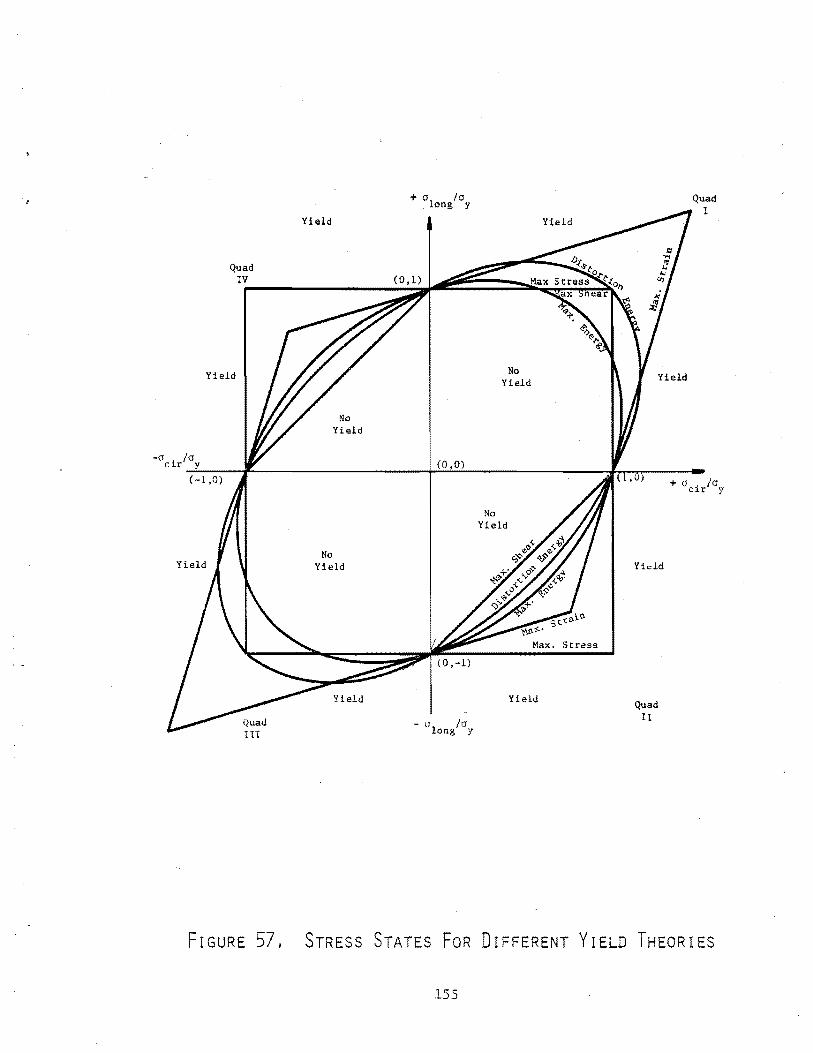
+ a1

Ia ong y

Yield Yield

Quad

IV~------------~~~~====~~~~~

1 /a

r Y

Yield

( -1,0)

No Yield

No Yield

(0,0)

- n 1 Ia ong y

No Yield

No Yield

Max. Stress

Yield

Quad 1

Yield

Yidd

Quad II

+a . /a c:~r Y

FIGURE 57, STRESS STATES FoR DIFFERENT YrELD THEORIES

155

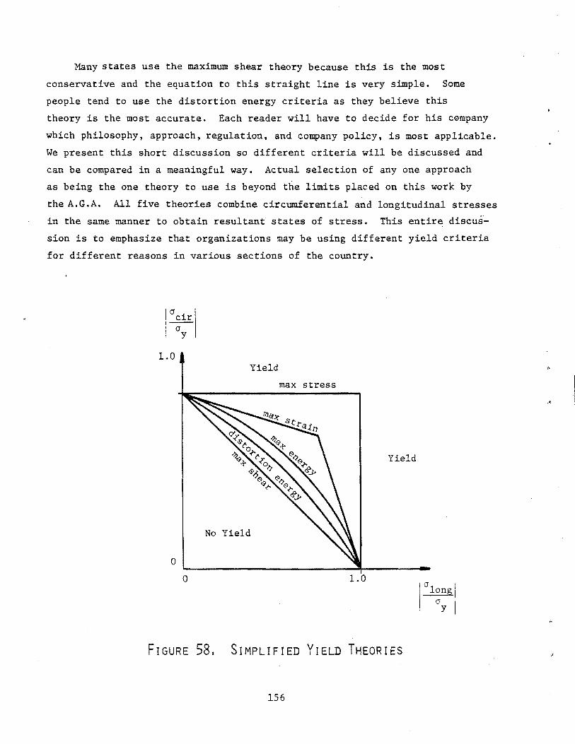
Many states use the maximum shear theory because this is the most

conservative and the equation to this straight line is very simple. Some

people tend to use the distortion energy criteria as they believe this

theory is the most accurate. Each reader will have to decide for his c0mpany

which philosophy, approach, regulation. and company policy, is most applicable.

We present this short discussion so different criteria will be discussed and

can be compared in a meaningful way. Actual selection of any one approach

as being the one theory to use is beyond the limits placed on this work by

the A.G.A. All five theories combine circumferential and longitudinal stresses

in the same manner to obtain resultant states of stress. This entire discus·­

sion is to emphasize that organizations may be using different yield criteria

for different reasons in various sections of the country.

!.

0

cir I' ' (J ; y

1.0 Yield

max stress

Yield

No Yield

0

0 1.0

I (J I

longi

. cry I

FIGURE 58. SIMPLIFIED YIELD THEORIES

156

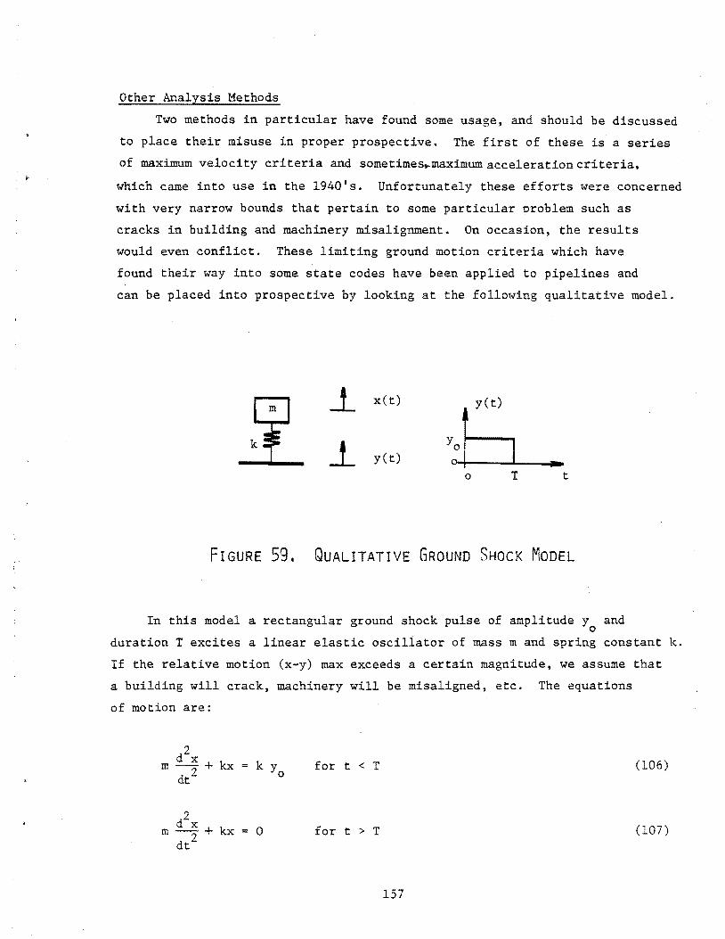
Other Analysis Methods

Two methods in particular have found some usage, and should be discussed

to place their misuse in proper prospective. The first of these is a series

of maximum velocity criteria and sometimes~maximumaccelerationcriteria,

which came into use in the 1940's. Unfortunately these efforts were concerned

with very narrow bounds that pertain to some particular problem such as

cracks in building and machinery misalignment. On occasion, the results

would even conflict. These limiting ground motion criteria which have

found their way into some state codes have been applied to pipelines and

can be placed into prospective by looking at the following qualitative model.

_l x(t) y(t)

j_ y(t) 0 T t

FIGURE 59. QuALITATIVE GRoUND SHOCK MoDEL

In this model a rectangular ground shock pulse of amplitude y and 0

duration T excites a linear elastic oscillator of mass m and spring constant k.

If the relative motion (x-y) max exceeds a certain magnitude, we assume that

a building will crack, machinery will be misaligned, etc. The equations

of motion are:

2 m d x + kx k y for t < T (106)

dt2 0

2 m d x + kx = 0 for t > T (107)

dt 2

157

dx The initial conditions are at time t=O, x=O, and = 0. Solving these dt

equations for these initial conditions gives:

y 0

(x-y) max

y 0

(x-y) max

= 0.5 esc

= 0.5

if/F T < IT m

(108)

if/K T > II m -

(109)

For short durations esc jFT · 1 1~ 2 d m 2 approxl.Illate y equa s k T an :

II (Y T) m o

(x-y)max = 1.0 if r:E_" T < II m -3

(110)

.For a specific structure k, m, and (x-y) are constants. This means that if

~ T >IT then y is equal to a constant and is a threshold for damage and for ~T:ll o V~ - 3, (y

0T) is equal to another constant and is also this threshold.

Usually investigators present what amounts to these same results by present-

ing results 180° out of phase.

velocity corresponds to the time

made by multiplying and dividing

In 1942 the Bureau of Hines

Acceleration corresponds to displacement and

integral of displacement if this shift is

by k, a constant for a specific structure. m , [13] conducted experiments because of

damage and litigation arising from blasting. In these tests, displacements

were recorded for 10- to 10,000-lb charges at standoff distances from 100

to 6000 ft. Criterion for failure in surface buildings were the development

of cracks in plaster. The Bureau of Mines investigators concluded that

ground accelerations less than 0.1 g's would not cause damage, accelerations

between 0.1 and 1.0 g's were in a caution range, and accelerations greater

than 1.0 g's were dangerous. These were fairly long dura~i~~esults with

frequencies up to 10 cps. As already noted, an acceleration criterion applies

for long duration results.

In 1949, Crandell [20] proposed a constant velocity (short duration)

criterion for protecting structures from blasting. His lower limit for

158

•J

caution to structures correponds to a peak soil particle velocity of 3.0 in/sec.

Crandell then created an arbitrary formula to relate this velocity to standoff

distance, charge weight, and a ground transmission constant.

The present U. S. Bureau of Mines criteria [21] for blasting safety

involve both a limiting soil particle velocity of 2 in/sec below 3 H~ and

limiting ground acceleration of 0.10 g's above 3 Hz. Obviously these criteria

are an effort to meet both low frequency and high frequency limiting conditions.

These criteria developed for buildings have been applied to pipelines

under the assumptions that it does not matter if the structure is buried

(incorrect because of the mass of soil which acts with the structure) and a

pipe can be considered as a structure similar to a building (a very crude

assumption).

By way of summary, this first velocity and acceleration criteria have

some validity for building, but none at all for buried p.ipe. They also are

often misapplied because people often ignore the ~Tor frequency limitations. m

The second effort in common use is called the Battelle formula [22].

It uses the Morris [10] equation for ground motion, and assumes that the

pipeline movements equal those of the surrounding soil. These assumptions

lead to a~ analysis and permits no diffraction of the shock front

around the pipe. The equation for circumferential stress is given by

where

C1 cir

K is

E is

w is

R is

D is

h is

C1 cir

= 4 • 26 K E h f"W R D2

a site factor to account

pipe modulus (psi)

charge weight (lbs)

standoff distance (ft)

pipe diameter (in)

pipe thickness (in)

is circumferential stress

(111)

for soil conditions

(psi)

Figure 60 shows a plot of test data versus this equation. To be perfectly

fair, this evaluation is not a proper one because the authors state that

Equation (111) is not valid for standoff distances less than 100 ft.

159

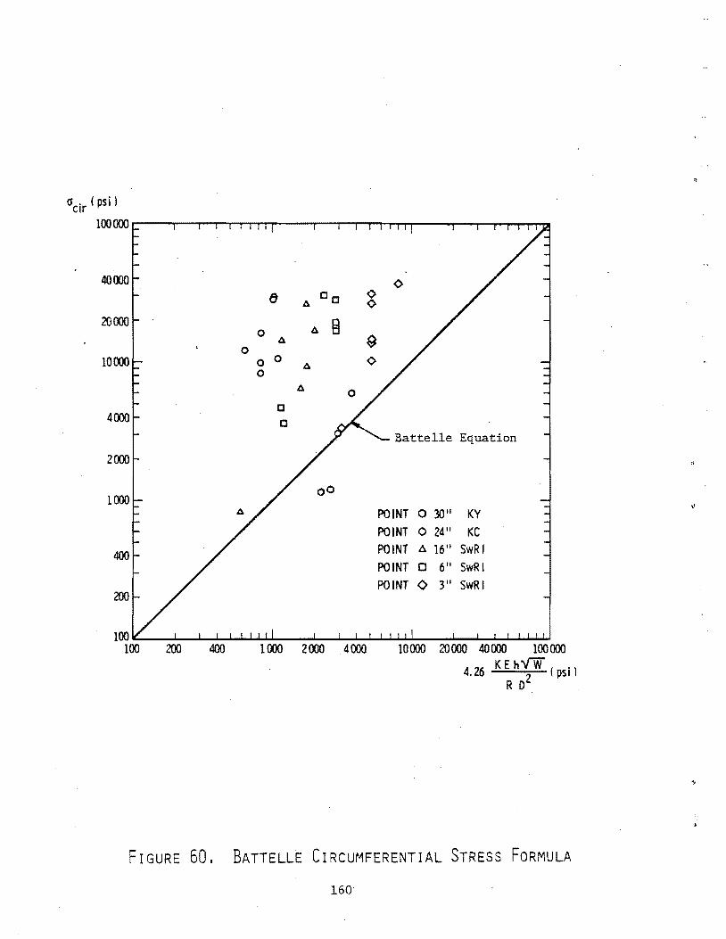
FIGURE 60. BATTELLE CIRCUMFERENTIAL STRESS FORMULA

160

Nevertheless this comparison is made because users have ignored the author's

qualifying statement and have used the results. Equation (111) is not as

accurate as our new relationships. In addition, misuse does not give

conservative results as Figure 60 shows, as the measured stresses are

higher than the predicted ones. Even if this formuli were applied for

standoff distances greater than 100 feet, its use would be questionable.

Equation (111) shows that doubling the pipe thickness while keeping every­

thing else constant doubles the stress in the pipe. This conclusion cannot

be explained. Increases in pipe thickness h are expected to reduce the

stress cr . . c~r

A company's ability to use the results in this report may be restricted

by regulations based on ground motion limitations or other criteria. When

these circumstances arise, the reader should probably use both this report

and the regulations, so blasting conditions can at least be limited to which­

ever gives the most conservative result.

Factor of Safety

The second question which must be faced by each company is "what factor

of safety will we use?" This report will not answer this question either, but

some guidance will be given.

No one number should be used as a factor of safety because many interac­

tions are involved. Most newer pipes are manufactured from ductile materials,

but some older pipes were manufactured from brittle materials. A ductile

material can strain well beyond yield and still exhibit very little deforma­

tion. On the other hand, a brittle pipe material cannot exceed yield at all

or the pipe will crack. Obviously the consequence of yielding is much more

severe in a brittle than in a ductile pipeline, so much larger safety factors

should be used in brittle as opposed to ductile pipelines.

One standard deviation for predicting both circumferential and longi­

tudinal stresses from blasting equals essentially 45% of the predicted value

(46% for circumferential stress and 44% for longitudinal stress). This

statement infers that were the same blasting against pipeline experimental

conditions repeated a large number of times, approximately 68% of the

results would fall between [1±0.45] times the predicted value, and 95% of

the results would fall between [1±0.90] times the predicted value. This

161

prediction of scatter assumes a normal distribution of test results which

is not quite true, and it applies only to those stress components caused

by blasting.

Knowing a standard deviation for the blasting components of stress

helps, but it alone cannot determine the safety factor. Another key

consideration is the magnitude of the blasting stresses relative to the

total stresses. For example, in a pipeline with a yield stress of 60 ksi,

a blasting stress of 10 ksi means one standard deviation is ± 4.5 ksi;

whereas, a blasting. stress of 40 ksi means one standard deviation is 18 ksi ..

Obviously one standard deviation of 4.5 ksi is fairly insignificant relative

to a 60 ksi yield point especially when compared to one standard deviation

of 18 ski relative to 60 ksi. The magnitude of the blasting stress relative

to the total state of stress must be considered in selecting an appropriate

safety factor.

One final consideration in the selection of a safety factor is some

concept of the consequences of failure. Loss of service in a major pipeline

serving an entire region of the United States has to be more serious than

loss of service in an artery into some building development. This observation

implies that factor of safety might be presented as a function of pipe

diameter because the larger lines are usually the most important ones.

As should be apparent by this discussion, factor of safety is not a

one answer question. We must leave this consideration up to each individual

company as regulations and company policy can also differ in various sections

of the country.

162

. i

. (

••

IX CONCLUSIONS AND RECOMMENDATIONS

The following conclusions are reached from this program:

(1) The functional relationships developed in this report represent a

general solution to predict the maximum stress of a buried pipe to

nearby point and line explosive sources in various types of soils.

The final solution derived in Section VI uses both approximate

analyses procedures to interrelate variables and empirical test

results to develop the final functional format. Only elastic procedures

were used because it was considered unacceptable to permit any stress

to exceed yield in a pipeline.

(2) The general solution to predict the pipe stresses from underground

detonation requires knowledge of the maximum radial soil displacement.

This relationship is needed because the ground motion defines the forc­

ing function applied to a buried pipe from blasting.

(3) Equations for predicting soil particle velocity and displacement for

a wide range of single underground explosion energies (i.e. point

sources), soils, and standoff distances were derived empirically

applying SwRI as well as other investigation data, and are given

in equations (30) and (31).

(4) Equations (44) and (45) give the functional relationships for particle

velocity and soil displacement for line sources (i.e. multiple

detonation). Again, these equations were obtained empirically using

SwRI measurements reported in Section IV.

(5) Functional relationships to predict the pipe response to near under­

ground detonations were derived for point and line sources and are

presented in equations (91), (94) (95a) and (95b), for circumferential

and longitudinal stresses. These close form solutions were obtained

from the experiments reported in Section III and IV of this report.

163

(6) The empirical data used to derive equation (95a) and (95b) infer that

a change in mode of pipe response occurs around a cr of 26 7 5 psi, which

has a very pronounced effect on longitudinal response and only a small

effect on circumferential response.

(7) Analytical and experimental observations on 3-, 6-, 16-, 24- and

30-in.diameter pipe revealed that stresses were independent of both

the pipe length and the pipe radius. Static analysis procedures do

not yield this conclusion, and cannot be used to draw valid conclusions

in this dynamic problem.

(8) The sensitivity analysis given in Section VIII, Table XX indicated

that pipe stresses are most sensitive to standoff distance R and least

sensitive to pipe properties (i.e. modulus of elasticity E and

thickness h). Changes in the standoff distance also have a greater

influence on the stress for a point source than a line source.

(9) The general solution is also independent of soil density p, and seismic

P-wave velocity c, in the soil. These soil properties mathematically

cancel out of the analysis in Section VI because a simplified linear

approximation was used to interrelate soil displacement, soil proper­

ties, standoff distance and energy release. Had the more complex

hyperbolic tangent relationship given in equation (30) been used, the

circumferential and longitudinal stresseswould become weak functions of p

and c. The simplified format was used because adequate engineering

answers were obtained without appreciable benefit from added complexity.

(10) From the experimental data and analysis presented in this report, it

was shown that ground motions and pipe response parameters from

transient pulses can be scaled or modeled. This observation was

verified with experiments at three different test sites in three

different states using pipes with diameters ranging from 3 to 30 in.

(11) A knowledge of the state of stress caused by blasting is necessary but

not sufficient information to determine if a buried pipe will yield.

164

•I

/"

/

Other stresses such as those caused by internal pipe pressurization,

thermal expansion or contraction, surcharge or overburden, and

residual stress from welding and other assembly processes can be

very significant. This program does not include a discussion of states

of stress from other cause. However, an accurate estimate of the

elastic state of stress can be made by superposition through additions

of stresses with their signs considered. After the resultant

longitudinal and circumferential stresses have been obtained a

failure theory for yielding will have to be selected to determine if

the pipe survives. Some of these theories are discussed in Section VIII.

(12) Other analytical methods have been used in the past to predict struc­

tural response from underground detonation. Two methods in particular

have found some usage. The first of these is a series of maximum

soil velocity criteriat and sometimes acceleration criteria. The

second is called the Battelle formula, which is based on Morris'

equation for ground motion, and assumes that the pipeline movements

equal those of the surrounding soil. The first criteria have some

validity for surface structures such as buildings, but none at all for

buried pipes. It is often misused because people find it easy to

apply in spite of its limited applicability. The second criteria bv

the author's own admissions are not valid for standoff distances of

less than 100 ft. However, users have ignored this limitation and have

applied the results for much closer standoff distance, thereby predict­

ing quite often lower stresses than those measured in this program.

The Batelle formula (e~ 111) is also suspect since it yields the

questionable conclusion that doubling the pipe thickness while keeping

everything else constant doubles the stress in the pipe.

(13) The use of the results from this report may be restricted by regulatory

codes based on either ground motion limitations and/or Batelle formula.

When this circumstance arises, the reader should use both this report

and regulatory codes, so blasting conditions can at least be limited

to whichever gives the most conservative results.

165

(14) What factors of safety can be used in applying these results is not

answered, because many interactions are involved. The following

factors interplay:

a. Pipe ductility b. Magnitude of the blasting stresses relative to the total ·stress c. Failure theories used d. Consequences of failure e. Regulations and codes f. Company policy g. The charge should be buried at a standoff distance of 1.5

or greater pipe diameters from the center of the pipe.

Factor of safety considerations are to be determined by individual

users.

(15) One standard deviation for predicting both circumferential and longi­

tudinal stresses from blasting equals essentially ± 45% of the

predicted value (46% for circumferential stress and 44% for longi­

tudinal stress). This statistic infers that if a large number of the

same blasting conditions were to be repeated, approximately 68% of

the results would fall between [1 ± 0.45] times the predicted value,

and 95% of the results would fall between [1 ± 0.90] times the

predicted value. This calculation assumes a normal distribution of

the test results and applies only to those stress components caused

by blasting.

(16) Assumptions and limitations associated with the general solution are:

(a) The charge and the center-line of the pipe are at the same depth.

(b) A line charge is a continuous line rather than a series of point charges. A point source has no shape or finite size.

(c) Any line source runs parallel to the pipeline.

(d) The pipeline is straight without elbows or valves.

(e) Wrapping, sand beds, and other potential shock isolation layers between the pipe and the soil have no effect.

(f) The solution gives only the elastic stress contributions from blasting. No inelastic behavior is included in this solution.

(g) Explosive sources always detonate instantly.

(h) Reflections from the surface of the ground are insignificant.

(i) No explosive energy (or at least a constant percentage of the energy) goes into cratering, air blast, and other phenomena.

166

·'

, ..

.{

(j) Explosive charge and pipe are embedded in the same soil medium.

(k) Some conclusions for minimum standoff for application.

Because of the above limitations the following recommendations are

made for additional investigation to improve the validation of these

program results and broaden the usefulness of the data.

(1) Conduct additional scale model tests to examine the results of blasting when the explosive charge is well below the center line of the pipe and no energy is vented to the atmosphere.

(2) Conduct model tests in which the charge and pipeline are in different soil mediums to determine if any ground shock reflections occur which appreciably invalidate the analysis.

(3) Develop procedures to model an explosive grid system and verify through model tests.

167

X. REFERENCES

1. Wilfred E. Baker, Peter S. Westine, and Franklin T. Dodge, Similarity Methods in Engineering Dynamics, Spartan Division of Hayden Books, Rochelle Park, N.J., 1978.

2. H. L. Langhaar, Dimensional Analysis and Theory of Models, John Wiley and Sons, New York, 1951.

3. G. Murphy, Similitude in Engineering, Ronald Press, New York, 1950.

4. L. I. Sedov, Similarity and Dimensional Methods in Mechanics, Edited .. by Maurice Holt, translated from Russian to English by Morris Feldman, Academic Press, New York, 1959.

5. D. S. Carder and W. K. Cloud, "Surface Motion from Large Underground Explosions," Journal of Geophysical Research, Vol. 64, No. 10, October 1959, pp. 1471-1487.

6. F. J. Crandell, "Transmission Coefficient for Ground Vibrations Due to Blasting," Journal of Boston Society of Civil Engineering, Vol. 47, No. 2, April 1960, pp. 152-168.

7. G. M. Habberjam and J. T. Whetton, "On the Relationship Between Seismic Amplitude and Charge of Explosive Fired to Routine Blasting Operations," Geophysics, Vol. 17, No. 1, January 1952, pp. 116-128.

8. D. E. Hudson, J. L. Alford, and W. D. Iwan, "Ground Accelerations Caused by Large Quarry Blasts," Bulletin of the Seismic Society of America, Vol. 51, No. 2, April 1961, pp. 191-202.

9. Ichiro Ito, "On the Relationship Between Seismic Ground Amplitude and the Quantity of Explosives in Blasting," reprint from Memoirs of the Faculty of Engineering, Kyoto University, Vol. 15, No. 11, April 1953, pp. 579-587.

10. G. Morris, "The Reduction of Ground Vibrations from Blasting Operations, Engineering, April 21, 1950, pp. 430-433.

11. N. Ricker, "The Form and Nature of Seismic Waves and the Structure of Seismograms," Geophysics, Vol. 5, No. 4, October 1940, pp. 348-366.

12. G. A. Teichmann and R. Westwater, "Blasting and Associated Vibrations," Engineering, April 12, 1957, pp. 460-465.

13. J. R. Thoenen and S. L. Windes, "Seismic Effects of Quarry Blasting," Bureau of Mines Bulletin 442, 1942, pp. 83.

14. D. E. Willis and J. T. Wilson, "Maximum Vertical Ground Displace­ment of Seismic Waves Generated by Explosive Blasts," Bulletin of the Seismic Society of America, Vol. 50, No. 3, July 1960, pp. 455-459.

168

15. B. F. Murphey, nParticle Motions Near Explosions in Halite,'' Journal of Geophysical Research, Vol. 66, No. 3, March 1961, pp. 947ff.

16. H. Nicholls, C. Johnson, and W. Duvall, "Blasting Vibrations and Their Effects on Structures," Final Report 1971, Denver Mining Research Center for Bureau of Mines, BuMines Report No. B 656, PB 231 971.

17. Anon., Project Dribble Salmon, nAnalysis of Ground Motion and Containment, Roland F. Beers, Inc. report to Atomic Energy Commission on Tests in Tatum Salt Dome, Mississippi, Final Report VUF-1026, November 30, 1965.

18. W. M. Adams, R. G. Preston, P. L. Flanders, D. C. Sachs, and W. R. Perret, "Summary Report of Strong-Motion Measurements, Underground Nuclear Detonations," Journal of Geophysical Research, Vol. 66, No. 3, March 1961, pp. 903ff.

19. Stephen Timoshenko, Strength of Materials, Part II: Advanced Theory and Problems, Third Edition, Van Nostrand Company, Princeton, New Jersey, March 1956.

20. F. J. Crandell, "Ground Vibrations Due to Blasting and Its Effect Upon Structureslf, Journal Boston Soc. Civil Engineers, Vol. 36, 1949, p 245.

21. J. F. Wiss, "Effects of Blasting Vibrations on Buildings and People", Civil Engineering, July 1968, pp. 46-48.

22. George M. McClure, Thomas V. Atterbury, and Noah A. Frazier, "Analysis of Blast Effects on Pipelines", Journal of the Pipeline Division, Proceeding of the American Society of Civil Engineers, November 1964.

169

English

A

CD

c (ft/sec)

D (in)

d

dx

E (psi)

F,L,T

I

i

i s

J (in 4)

K

KE

k

i (ft)

m

n

XI. LIST OF PARAMETERS AND SYMBOLS

Projected pipe area; peak amplitude for either velocity or displacement

Acceleration

Diffraction coefficient

Seismic P-wave velocity in soil

Pipe diameter

"Dim,ensionally equal to"

Differential length of pipe

Modulus of elasticity for the pipe material

Fundamental units of measure; force, length and time, respectively

Symbol for function of

Pipe wall thickness

Total applied impulse

Any applied specific impulse

Side-on specific impulse

Second moment of area

Site factor for soil condition; a constant

Kinetic energy

Spring constant in the qualitative structural response model

Length of explosive line (for uniform charges spaced equal distances apart, this length is the spacing between charges times the number of charges)

Ratio of impulse or pressure on the back of the pipe relative to impulse or pressure at the front of the pipe; also mass in the qualitative structural response mode.

Numerical constants

170

English

nW

p 0

(psf)

Ps

R (ft)

R1

, ~ (ft)

r (in)

s

SC (psi)

SE (in-lb)

SE . (in-lb) c~r

SE long

SL (psi)

T

t

U (ft/sec)

U/C

v

w (ft-lb)

W/9-~ft;tlb) w

0

X (ft)

X/R

Equivalent explosive energy release, see Equation (90) (lb AN-FO) and pp. 124 and 129.

Atmospheric pressure

Side-on pressure

Standoff distance from the center of the pipe to the charge

Distance between charge and ground motion canister

Pipe radius

One standard deviation as a percentage

Circumferential stress

Strain energy

Circumferential strain energy

Longitudinal strain energy

Longitudinal stress

Time constant associated with duration of the load

Variable constant

Maximum radial peak particle velocity of the soil

Maximum radial particle velocity of the soil at location 1, 2 ... (in/sec)

Particle velocity of soil obtained from accelerometer measure­ment at location 1

Scaled velocity

Velocity of shock front

Energy released in an explosive point source; charge weight

Energy released per unit length in an explosive line source

Mid-span deformation

Maximum radial displacement of the soil

Scaled displacement

171

English

X (in)

x-y (in)

y (in)

y (in) 0

Maximum radial displacement of the soil obtained by inte­grating the velocity at location 1

Displacement in the qualitative structural response model

Relative motion

Assumed deformed shape

Ground shock pulse of amplitude; threshold for damage

172

'I

.. \

. ;,)•

1'.!

- .

Greek Symbols

I Ct.l ... ' Ct.lQ

P' 8

A

J1

JlE;

1T term

( lb-sec2) P' Ps' 4

Pa (lb-sec~) pc2

ft4 (psf)

Pcp8 (psf)

pp

cr (psi)

cr cir(psi)

along (psi)

crmax (psi)

cr obs (psi)

cr cal (psi)

cry (psi)

T (sec)

w (rad/sec)

ll (psf)

• '

Exponents on parameters in the equation of dimensional homogeneity

Ang.le (see Figure 49)

Geometric scale factor

Mass per unit length

Micro strains

Dimensionless group

Mass density of soil or rock

Density behind the shock front

Compressibility of the soil

Heat capacity times temperature increase

Mass density of pipe

Maximum circumferential stress for values <2675 psi

Maximum circumferential stress in the pipe

Maximum longitudinal stress in the pipe

Maximum pipe stress; may be either the longitudinal or circumferential direction

Observed stress

Calculated v~lue

Yield point for the pipe

Period of pipe response

Fundamental natural frequency

Density times the heat of fusion

173