Embed Size (px)
Citation preview
Analysis of Alfalfa Production in a Water-Stressed Region:
A Dynamical Modeling Approach
by
Booyoung Kim
A Thesis Presented in Partial Fulfillment of the Requirements for the Degree
Master of Arts
Approved April 2015 by the Graduate Supervisory Committee:
Rachata Muneepeerakul, Chair
Benjamin Ruddell Rimjhim Aggarwal
ARIZONA STATE UNIVERSITY
May 2015
i
ABSTRACT
Alfalfa is a major feed crop widely cultivated in the United States. It is the fourth
largest crop in acreage in the US after corn, soybean, and all types of wheat. As of 2003,
about 48% of alfalfa was produced in the western US states where alfalfa ranks first,
second, or third in crop acreage. Considering that the western US is historically water-
scarce and alfalfa is a water-intensive crop, it creates a concern about exacerbating the
current water crisis in the US west. Furthermore, the recent increased export of alfalfa
from the western US states to China and the United Arab Emirates has fueled the debate
over the virtual water content embedded in the crop. In this study, I analyzed changes of
cropland systems under the three basic scenarios, using a stylized model with a
combination of dynamical, hydrological, and economic elements. The three scenarios are
1) international demands for alfalfa continue to grow (or at least to stay high), 2) deficit
irrigation is widely imposed in the dry region, and 3) long-term droughts persist or
intensify reducing precipitation. The results of this study sheds light on how distribution
of crop areas responds to climatic, economic, and institutional conditions. First,
international markets, albeit small compared to domestic markets, provide economic
opportunities to increase alfalfa acreage in the dry region. Second, potential water
savings from mid-summer deficit irrigation can be used to expand alfalfa production in
the dry region. Third, as water becomes scarce, farmers more quickly switch to crops that
make more economic use of the limited water.
ii
ACKNOWLEDGMENTS
I have a lot of people to thank for their help in the past two years. Above all, I
would like to sincerely thank my advisor Dr. Rachata Muneepeerakul for his tremendous
encouragement and effort. This thesis would never have been completed without the
exceptional help from him.
I would also like to sincerely thank Drs. Ben Ruddell and Rimjhim Aggarwal for
sitting on my thesis committee. Your input and insight was always invaluable and
sharpened my thinking. I appreciate your time and patience.
Thanks so much my friends and family, all for your support!
iii
TABLE OF CONTENTS
Page
LIST OF TABLES ..................................................................................................................... iv
LIST OF FIGURES .................................................................................................................... v
CHAPTER
1 INTRODUCTION ................. ....................................................................................... 1
2 BACKGROUND ................... ....................................................................................... 9
3 METHOD ....................... ........................................................................................... 15
3.1 Model Framework .............................................................................. 15
3.2 Model Description.............................................................................. 16
4 RESULTS ...................... ............................................................................................ 27
4.1 Baseline Model .................................................................................. 28
4.2 Three Scenarios ................................................................................. 30
4.3 Simulation Results ............................................................................. 33
5 CONCLUSION AND DISCUSSION .......................................................................... 36
REFERENCES....... ............................................................................................................... 40
APPENDIX
A LIST OF SYMBOLS AND DEFAULT PARAMETER VALUES ............................. 43
B MATLAB CODE ....................................................................................................... 46
iv
LIST OF TABLES
Table Page
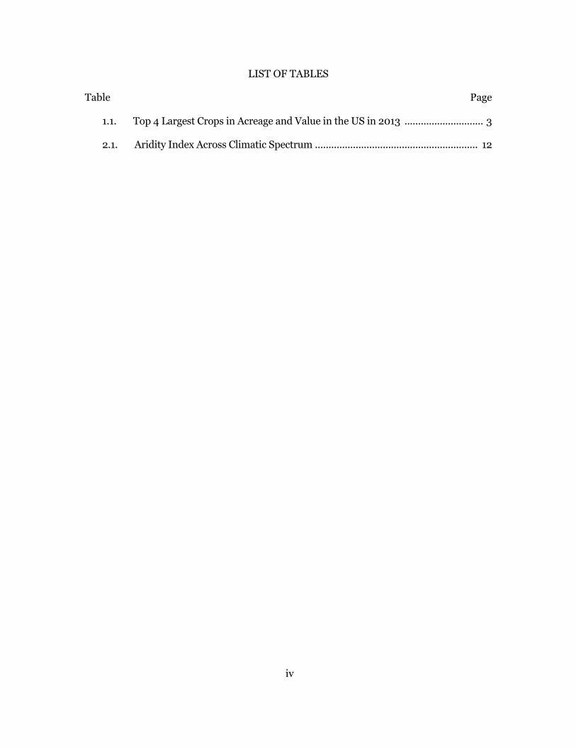
1.1. Top 4 Largest Crops in Acreage and Value in the US in 2013 ............................. 3
2.1. Aridity Index Across Climatic Spectrum ............................................................ 12
v
LIST OF FIGURES
Figure Page
1.1. Harvested Acres of Alfalfa Hay in 2012 ........................................................ 1
1.2. Acreage of Irrigated Harvested Cropland as Percent of All Harvested Cropland
Acreage in 2012 .......................................................................................... 4
1.3. Harvested Acreages of Irrigated Alfalfa Hay in 2012 ................................... 4
1.4. Partitioning of Green and Blue Water Consumption of Alfalfa ................... 4
1.5. Alfalfa Acreage Changes in the Western States and Non-Western States from
2003 to 2014 .............................................................................................. 7
1.6. Change in Alfalfa Hay Acreage Harvested from 2007 to 2012 .................... 8
2.1. Acreage Change Devoted to Corn for Grain and Soybeans for Beans from 2007
to 2012 ....................................................................................................... 11
2.2. Harvested Acres of Vegetables in 2012 ....................................................... 11
3.1. Cropland-use Change Framework .............................................................. 16
3.2. Partition of Precipitation into Stream Runoff and Evapotranspiration ... 23
3.3. Budyko Curves of Alfalfa (𝑣𝐴=3) and Other Crops (𝑣𝐵=1.5) ..................... 24
4.1. Time Series of Fractions of Crop Areas and Crop Prices and Phase Plane of
Fractions of Crop Areas of the Baseline Case .......................................... 28
4.2. Alfalfa Hay Exports from 2007 to 2013 ..................................................... 30
4.3. Yield Response to Evapotranspiration for Alfalfa, Corn, Soybeans, Sunflowers,
and Winter Wheat .................................................................................... 32
4.4. Phase Portraits of Different Levels of International Demands for Alfalfa 33
4.5. Phase Portraits of Different Levels of Midsummer Deficit Irrigation in the Dry
Region ....................................................................................................... 34
4.6. Phase Portraits of Different Levels of Precipitation in the Dry Region .... 35
1
CHAPTER 1
INTRODUCTION
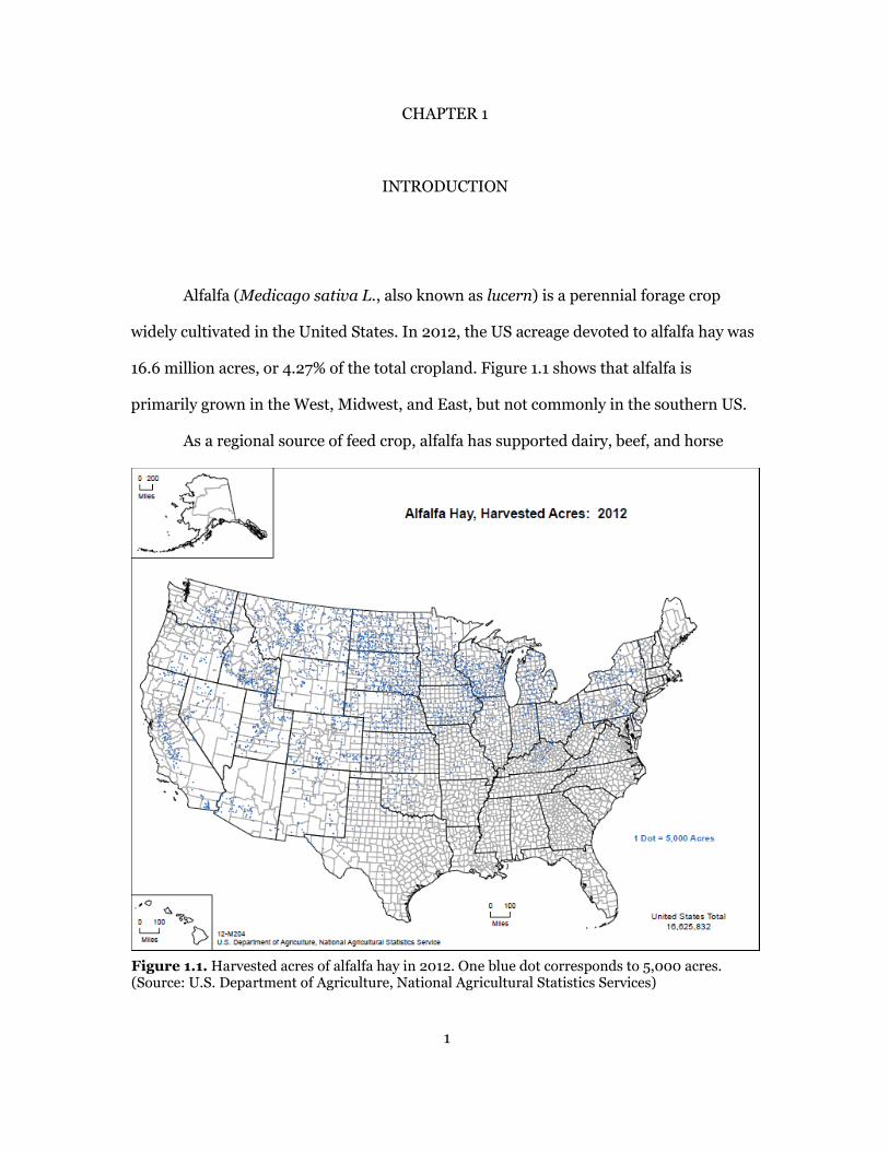
Alfalfa (Medicago sativa L., also known as lucern) is a perennial forage crop
widely cultivated in the United States. In 2012, the US acreage devoted to alfalfa hay was
16.6 million acres, or 4.27% of the total cropland. Figure 1.1 shows that alfalfa is
primarily grown in the West, Midwest, and East, but not commonly in the southern US.
As a regional source of feed crop, alfalfa has supported dairy, beef, and horse
Figure 1.1. Harvested acres of alfalfa hay in 2012. One blue dot corresponds to 5,000 acres. (Source: U.S. Department of Agriculture, National Agricultural Statistics Services)
2
industries in the US (Martin, Mertens, & Weimer, 2004). In particular, it has been an
important feed for dairy farms due to its high levels of protein and low fiber (Glennon,
2009; Robinson, 2014). According to Robinson (2014), alfalfa hay has the combination
of nutritional features beneficial for milk cows that most other feedstuffs do not possess.
Furthermore, when fed low-quality alfalfa, a dairy cow produces at least less than 50% of
its potential milk (Glennon, 2009). For this reason, alfalfa production is closely
associated with the dairy industry. Alfalfa utilization by dairy cows is about 75 – 80 % of
alfalfa usage in the leading dairy states such as California and Wisconsin (Summers et
al., 2008). As alfalfa will likely remain an irreplaceable portion of the diets for high milk
producing cows, the dairy industry is likely to drive alfalfa production in the future.
Apart from alfalfa’s role for dairy cows, it has several traits that make it attractive
to farmers. First, it is drought tolerant. Its deep root system allows it to draw on soil
moisture reserves in water-limited settings while improving soil structure (Confalonieri
& Bechini, 2004). Also, it has the ability to enter dormancy under continued dry
conditions. Once it is relieved from moisture stress, alfalfa recovers its normal growth
stage. These traits make it less susceptible than other crops to loss of yield caused by
extended dry periods (Bauder, Hansen, Lindenmeyer, Bauder, & Brummer, 2011).
Second, alfalfa is moderately salt tolerant. Soil salinity restricts crop growth and
subsequently reduces crop yield (Tanji & Kielen, 2002). Because farmers need to use
less water to leach salts from the soils when growing alfalfa, alfalfa is better adapted to
dry conditions with high soil salinity than other salt sensitive crops. Third, alfalfa has
high yields among other forage crops (Confalonieri & Bechini, 2004). In 2013, Arizona’s
alfalfa yield was 8.1 tons per acre, followed by California’s 6.8 tons per acre, while the
national average was 3.24 tons per acre. Fourth, alfalfa fixes nitrogen with its roots,
which improves soil fertility. Putnam et al. (2001) conservatively estimated that about
3
20% of alfalfa acreage is rotated to another crop each year in the US. In particular, it is
typically rotated with corn, wheat, and barley, as well as high-value crops such as
tomatoes and lettuce (Putnam et al., 2000). Moreover, because alfalfa can self-produce
nitrogen for itself, it does not require extra nitrogen fertilizer for optimal growth
(Putnam et al., 2001). Lastly, alfalfa is a key rotation crop capable of suppressing plant
disease. In general, alfalfa’s high level of adaptability and versatility is central to its wide
cultivation.
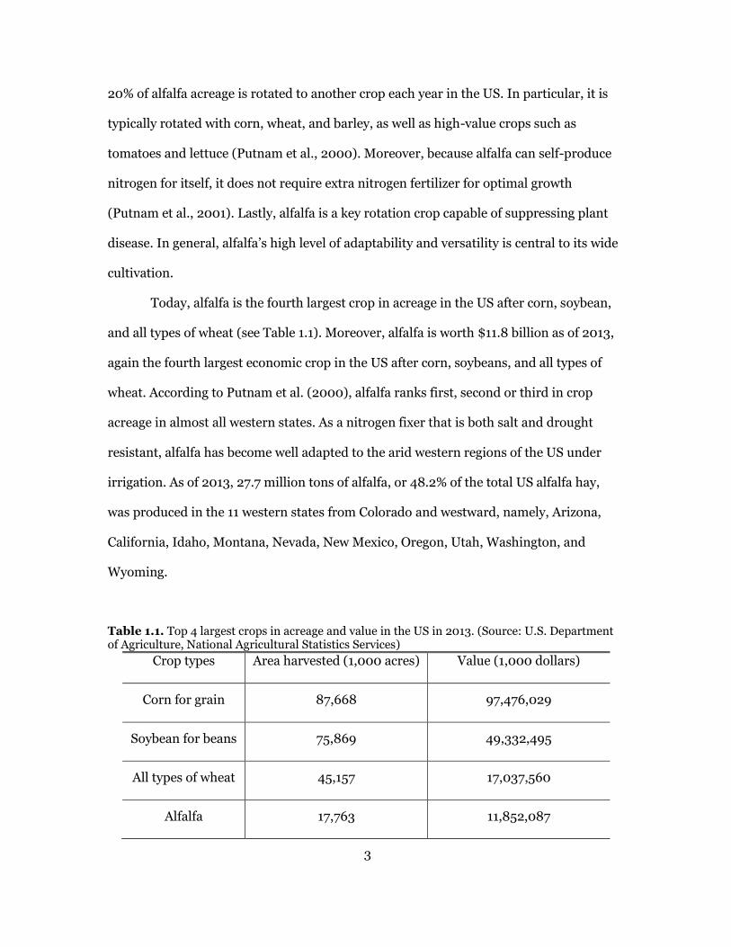
Today, alfalfa is the fourth largest crop in acreage in the US after corn, soybean,
and all types of wheat (see Table 1.1). Moreover, alfalfa is worth $11.8 billion as of 2013,
again the fourth largest economic crop in the US after corn, soybeans, and all types of
wheat. According to Putnam et al. (2000), alfalfa ranks first, second or third in crop
acreage in almost all western states. As a nitrogen fixer that is both salt and drought
resistant, alfalfa has become well adapted to the arid western regions of the US under
irrigation. As of 2013, 27.7 million tons of alfalfa, or 48.2% of the total US alfalfa hay,
was produced in the 11 western states from Colorado and westward, namely, Arizona,
California, Idaho, Montana, Nevada, New Mexico, Oregon, Utah, Washington, and
Wyoming.
Table 1.1. Top 4 largest crops in acreage and value in the US in 2013. (Source: U.S. Department of Agriculture, National Agricultural Statistics Services)
Crop types Area harvested (1,000 acres) Value (1,000 dollars)
Corn for grain 87,668 97,476,029
Soybean for beans 75,869 49,332,495
All types of wheat 45,157 17,037,560
Alfalfa 17,763 11,852,087
4
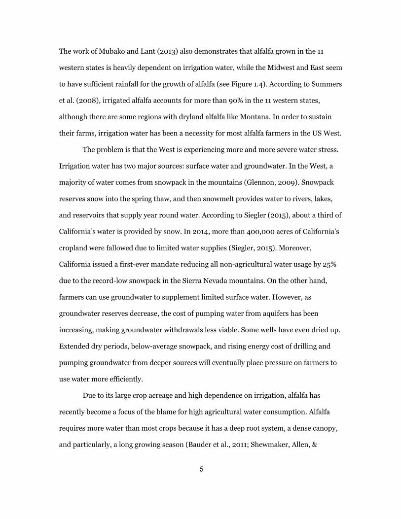
In most arid western states, however, the farming is almost impossible without
irrigation. Nationally, about 16.5% of the total harvested cropland was irrigated in 2012.
Figure 1.2 indicates that the majority of the western region relies on irrigation, along
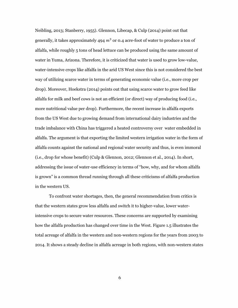
with the west side of the Mississippi River and some parts of Florida. In the case of
alfalfa, it was grown on 10.4% of irrigated land in the US in 2012, and most irrigated
alfalfa hay production was concentrated in the 11 western states (see Figure 1.3).
Figure 1.2. Acreage of irrigated harvested cropland as percent of all harvested cropland acreage in 2012. The relative magnitude is denoted by the progression of shades. As the percentage increases, the color deepens. (Source: U.S. Department of Agriculture, National Agricultural Statistics Services)
Figure 1.3. Harvested acreages of irrigated alfalfa hay in 2012. One blue dot corresponds to 2,000 acres. (Source: U.S. Department of Agriculture, National Agricultural Statistics Services)
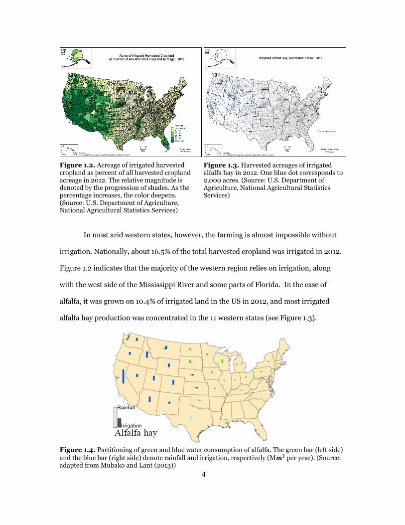
Figure 1.4. Partitioning of green and blue water consumption of alfalfa. The green bar (left side)
and the blue bar (right side) denote rainfall and irrigation, respectively (M𝒎𝟑 per year). (Source: adapted from Mubako and Lant (2013))
5
The work of Mubako and Lant (2013) also demonstrates that alfalfa grown in the 11
western states is heavily dependent on irrigation water, while the Midwest and East seem
to have sufficient rainfall for the growth of alfalfa (see Figure 1.4). According to Summers
et al. (2008), irrigated alfalfa accounts for more than 90% in the 11 western states,
although there are some regions with dryland alfalfa like Montana. In order to sustain
their farms, irrigation water has been a necessity for most alfalfa farmers in the US West.
The problem is that the West is experiencing more and more severe water stress.
Irrigation water has two major sources: surface water and groundwater. In the West, a
majority of water comes from snowpack in the mountains (Glennon, 2009). Snowpack
reserves snow into the spring thaw, and then snowmelt provides water to rivers, lakes,
and reservoirs that supply year round water. According to Siegler (2015), about a third of
California’s water is provided by snow. In 2014, more than 400,000 acres of California’s
cropland were fallowed due to limited water supplies (Siegler, 2015). Moreover,
California issued a first-ever mandate reducing all non-agricultural water usage by 25%
due to the record-low snowpack in the Sierra Nevada mountains. On the other hand,
farmers can use groundwater to supplement limited surface water. However, as
groundwater reserves decrease, the cost of pumping water from aquifers has been
increasing, making groundwater withdrawals less viable. Some wells have even dried up.
Extended dry periods, below-average snowpack, and rising energy cost of drilling and
pumping groundwater from deeper sources will eventually place pressure on farmers to
use water more efficiently.
Due to its large crop acreage and high dependence on irrigation, alfalfa has
recently become a focus of the blame for high agricultural water consumption. Alfalfa
requires more water than most crops because it has a deep root system, a dense canopy,
and particularly, a long growing season (Bauder et al., 2011; Shewmaker, Allen, &
6
Neibling, 2013; Stanberry, 1955). Glennon, Libecap, & Culp (2014) point out that
generally, it takes approximately 494 𝑚3 or 0.4 acre-foot of water to produce a ton of
alfalfa, while roughly 5 tons of head lettuce can be produced using the same amount of
water in Yuma, Arizona. Therefore, it is criticized that water is used to grow low-value,
water-intensive crops like alfalfa in the arid US West since this is not considered the best
way of utilizing scarce water in terms of generating economic value (i.e., more crop per
drop). Moreover, Hoekstra (2014) points out that using scarce water to grow feed like
alfalfa for milk and beef cows is not an efficient (or direct) way of producing food (i.e.,
more nutritional value per drop). Furthermore, the recent increase in alfalfa exports
from the US West due to growing demand from international dairy industries and the
trade imbalance with China has triggered a heated controversy over water embedded in
alfalfa. The argument is that exporting the limited western irrigation water in the form of
alfalfa counts against the national and regional water security and thus, is even immoral
(i.e., drop for whose benefit) (Culp & Glennon, 2012; Glennon et al., 2014). In short,
addressing the issue of water-use efficiency in terms of “how, why, and for whom alfalfa
is grown” is a common thread running through all these criticisms of alfalfa production
in the western US.
To confront water shortages, then, the general recommendation from critics is
that the western states grow less alfalfa and switch it to higher-value, lower water-
intensive crops to secure water resources. These concerns are supported by examining
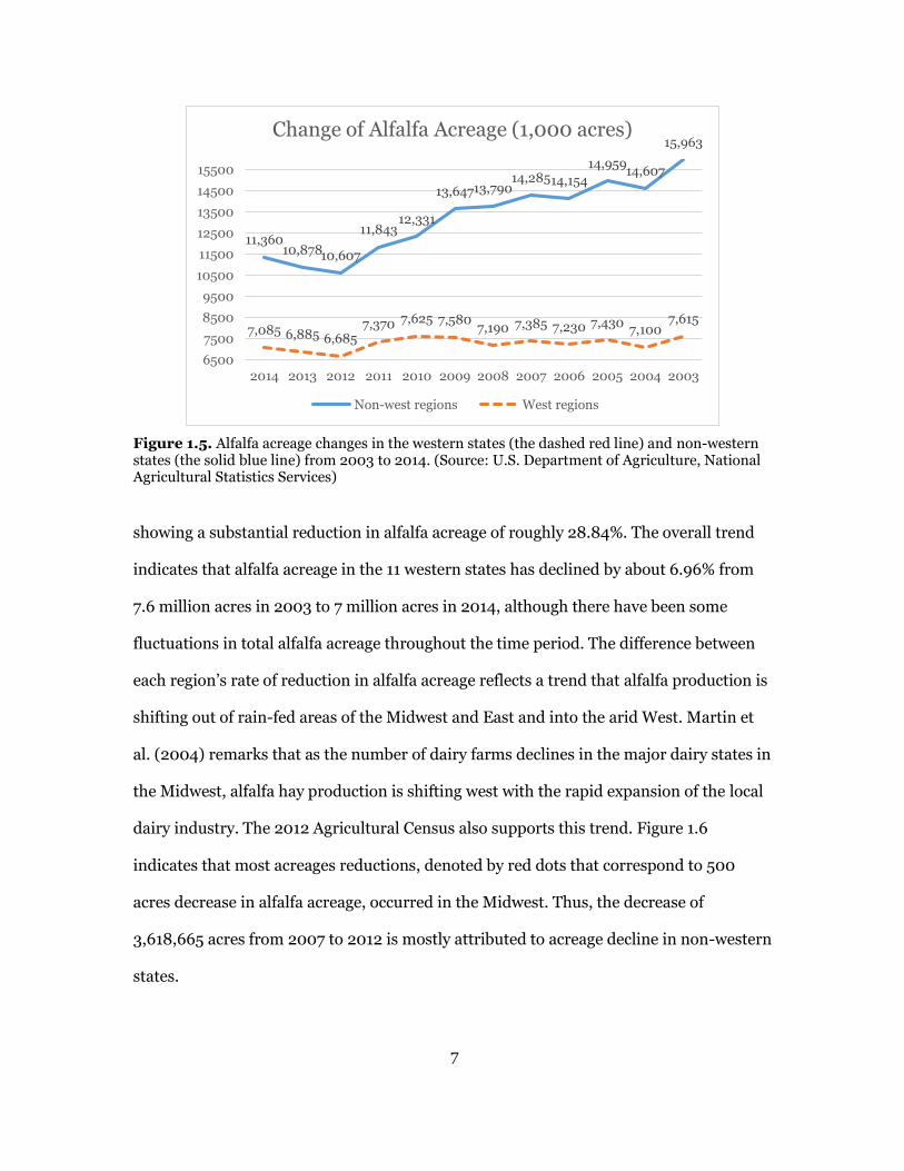
how the alfalfa production has changed over time in the West. Figure 1.5 illustrates the
total acreage of alfalfa in the western and non-western regions for the years from 2003 to
2014. It shows a steady decline in alfalfa acreage in both regions, with non-western states
7
showing a substantial reduction in alfalfa acreage of roughly 28.84%. The overall trend
indicates that alfalfa acreage in the 11 western states has declined by about 6.96% from
7.6 million acres in 2003 to 7 million acres in 2014, although there have been some
fluctuations in total alfalfa acreage throughout the time period. The difference between
each region’s rate of reduction in alfalfa acreage reflects a trend that alfalfa production is
shifting out of rain-fed areas of the Midwest and East and into the arid West. Martin et
al. (2004) remarks that as the number of dairy farms declines in the major dairy states in
the Midwest, alfalfa hay production is shifting west with the rapid expansion of the local
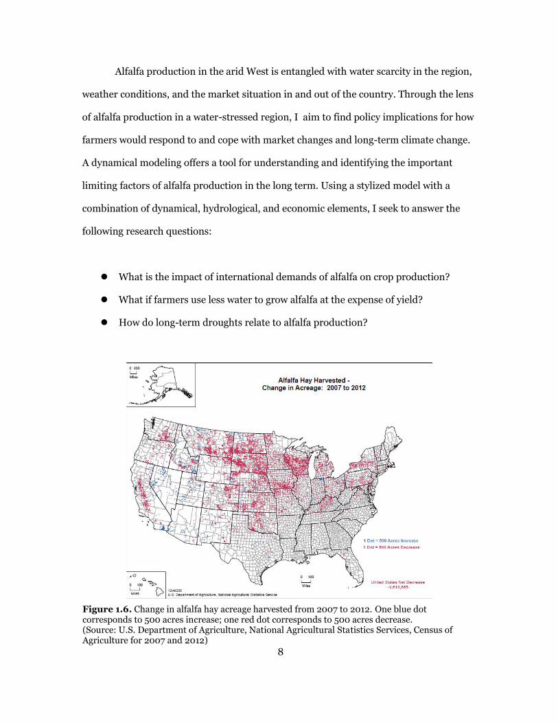
dairy industry. The 2012 Agricultural Census also supports this trend. Figure 1.6
indicates that most acreages reductions, denoted by red dots that correspond to 500
acres decrease in alfalfa acreage, occurred in the Midwest. Thus, the decrease of
3,618,665 acres from 2007 to 2012 is mostly attributed to acreage decline in non-western
states.
11,360 10,878 10,607
11,843 12,331
13,647 13,790 14,285 14,154
14,959 14,607
15,963
7,085 6,885 6,685 7,370 7,625 7,580
7,190 7,385 7,230 7,430 7,100
7,615
6500
7500
8500
9500
10500
11500
12500
13500
14500
15500
2014 2013 2012 2011 2010 2009 2008 2007 2006 2005 2004 2003
Change of Alfalfa Acreage (1,000 acres)
Non-west regions West regions
Figure 1.5. Alfalfa acreage changes in the western states (the dashed red line) and non-western states (the solid blue line) from 2003 to 2014. (Source: U.S. Department of Agriculture, National Agricultural Statistics Services)
8
Alfalfa production in the arid West is entangled with water scarcity in the region,
weather conditions, and the market situation in and out of the country. Through the lens
of alfalfa production in a water-stressed region, I aim to find policy implications for how
farmers would respond to and cope with market changes and long-term climate change.
A dynamical modeling offers a tool for understanding and identifying the important
limiting factors of alfalfa production in the long term. Using a stylized model with a
combination of dynamical, hydrological, and economic elements, I seek to answer the
following research questions:
What is the impact of international demands of alfalfa on crop production?
What if farmers use less water to grow alfalfa at the expense of yield?
How do long-term droughts relate to alfalfa production?
Figure 1.6. Change in alfalfa hay acreage harvested from 2007 to 2012. One blue dot corresponds to 500 acres increase; one red dot corresponds to 500 acres decrease. (Source: U.S. Department of Agriculture, National Agricultural Statistics Services, Census of Agriculture for 2007 and 2012)
9
CHAPTER 2
BACKGROUND
In this chapter, I contextualize the assumptions underlying the analysis.
Factors affecting alfalfa production
Alfalfa production is influenced by alfalfa price expectations, the profitability of
alternative crops, milk prices, the prices for corn and soybeans, and water availability
and costs (Butler, 2010). These factors are all incorporated into the model, except for the
expected prices of crops. In this study, farmers make production decision by maximizing
the profit from the use of a given cropland area. Profitable milk prices induce an increase
in the demand and price for alfalfa. Corn and soybeans are considered as the alternative
crops. Water availability and costs are major limiting factors of alfalfa production.
Only market valuation of alfalfa (i.e., value in exchange) is taken into
consideration for the purpose of this study. Alfalfa hay fed on farms (i.e., value in use) is
not considered in the model, which means that all produced alfalfa is marketed off the
farm. Because most alfalfa grown in the Midwest and East is fed on farms, this explains a
huge underestimation of alfalfa acreage in these regions in my analysis results. In
addition, the non-market values, such as rotation value for subsequent crops, scenic
value, and other environmental values, are excluded in the analysis. Thus, the model
results will be underestimated compared to actual data.
10
High/low-value crops
Alfalfa is, in general, classified as a low-value crop. That is, it is presumed that
alfalfa generates lower income per unit of land area than other crops such as specialty
crops (e.g., almond, lettuce, or broccoli). Provided that economics is the driving force of
cropping decisions, one would expect the initial response to be the dominance of high-
value crops over agricultural land. However, in reality, both low- and high-value crops
are grown on farms in tandem with each other. It reflects heterogeneity of various
conditions like climate and market risk, which enables alfalfa to “compete economically
for water and land resources directly and equally with all crops” even without subsidy
(Putnam, 2010). In economics, this coexistence of low- and high-value crops occurs
where marginal profit of producing low-value crops equals marginal profit of producing
high-value crops. In the analysis, high/low-value criterion is based on the comparison of
crop prices in relative terms, rather than using the conventional presumption of alfalfa as
a low-value crop in an absolute sense.
Alternative crops
The change in alfalfa acreage depends on the existence of profitable alternative
crops. Because virtually any crops cannot compete economically with urbanization and
industries for limited land and water resources, I exclude non-agricultural sectors from
the land-use change analysis. Only the agricultural sector competes for limited resources
in the model.
11
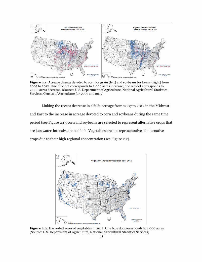
Linking the recent decrease in alfalfa acreage from 2007 to 2012 in the Midwest
and East to the increase in acreage devoted to corn and soybeans during the same time
period (see Figure 2.1), corn and soybeans are selected to represent alternative crops that
are less water-intensive than alfalfa. Vegetables are not representative of alternative
crops due to their high regional concentration (see Figure 2.2).
Figure 2.1. Acreage change devoted to corn for grain (left) and soybeans for beans (right) from 2007 to 2012. One blue dot corresponds to 2,000 acres increase; one red dot corresponds to 2,000 acres decrease. (Source: U.S. Department of Agriculture, National Agricultural Statistics Services, Census of Agriculture for 2007 and 2012)
Figure 2.2. Harvested acres of vegetables in 2012. One blue dot corresponds to 1,000 acres. (Source: U.S. Department of Agriculture, National Agricultural Statistics Services)
12
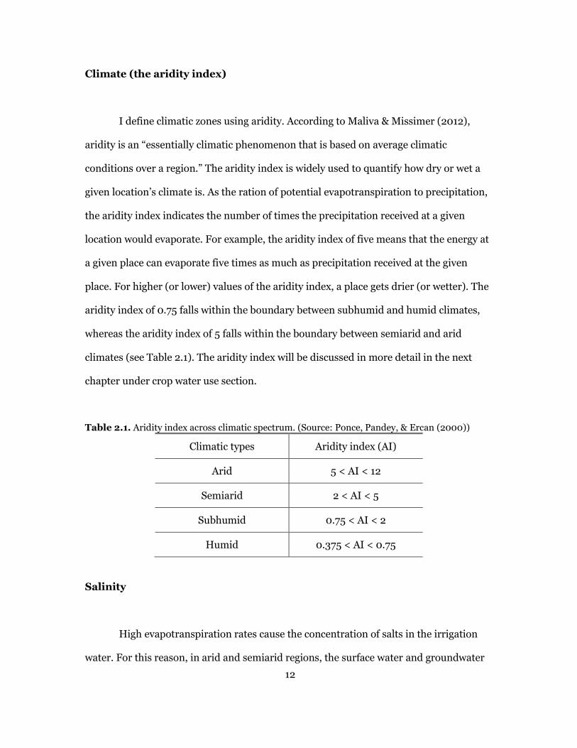
Climate (the aridity index)
I define climatic zones using aridity. According to Maliva & Missimer (2012),
aridity is an “essentially climatic phenomenon that is based on average climatic
conditions over a region.” The aridity index is widely used to quantify how dry or wet a
given location’s climate is. As the ration of potential evapotranspiration to precipitation,
the aridity index indicates the number of times the precipitation received at a given
location would evaporate. For example, the aridity index of five means that the energy at
a given place can evaporate five times as much as precipitation received at the given
place. For higher (or lower) values of the aridity index, a place gets drier (or wetter). The
aridity index of 0.75 falls within the boundary between subhumid and humid climates,
whereas the aridity index of 5 falls within the boundary between semiarid and arid
climates (see Table 2.1). The aridity index will be discussed in more detail in the next
chapter under crop water use section.
Table 2.1. Aridity index across climatic spectrum. (Source: Ponce, Pandey, & Ercan (2000))
Climatic types Aridity index (AI)
Arid 5 < AI < 12
Semiarid 2 < AI < 5
Subhumid 0.75 < AI < 2
Humid 0.375 < AI < 0.75
Salinity
High evapotranspiration rates cause the concentration of salts in the irrigation
water. For this reason, in arid and semiarid regions, the surface water and groundwater
13
generally contain more salts than in humid and subhumid regions. Also, saline soils are
naturally found in arid and semiarid regions. Soil salinity is a limiting factor of crop yield
because soluble salts at the root zone are harmful to plant growth (Shahid, Taha, &
Abdelfattah, 2013). Plants maintain their normal yield up to a certain threshold level of
root zone salinity, but after exceeding it, crop yield declines linearly with the increase in
the level of soil salinity. The degree of soil salinity is measured by using the electrical
conductivity of soil saturation extract (in units of deci-siemens per meter, 𝑑𝑆/𝑚).
Salinity issues will be explored in more detail in the next chapter under yield section.
The salt resistant characteristic of alfalfa is factored in the model as one of the
advantages of growing alfalfa in the arid regions. According to Tanji & Kielen (2002),
however, both alfalfa and corn are designated as moderately sensitive crops with salinity
threshold values of 2 𝑑𝑆/𝑚 and 1.7 𝑑𝑆/𝑚, respectively. Even though alfalfa is slightly
more salt tolerant than alternative crops of this study, the effect of soil salinity on crop
yield would not make a major difference in crop distribution.
Water costs
As discussed in the previous chapter, irrigation is generally necessary for alfalfa
production in arid western states, while irrigation is not widely used in humid
midwestern and eastern agricultural regions (see Figures 1.2, 1.3, and 1.4). Glennon
(2009) mentions that farmers in the West usually pay a few pennies for a thousand
gallons of water due to federally subsidized water and low-cost energy. In order to reflect
the underpriced water in the model, the cost of irrigation water is designed to be around
$15 per acre-foot, or $0.0006 per gallon of water in the West, while the water cost is set
to be close to zero in the rain-fed areas.
14
In this framework, because water is used on a farm, private goods aspect of water
is focused on the surface. First, more water consumption by one crop reduces the
amount of water available for other crops. This rivalry over water is coupled with
competition for land. In particular, it has a special significance in dry regions having
scarce water. Second, it is possible to effectively exclude farmers who do not pay for
water from water use. That is, farmers should pay for water whenever they use it,
otherwise, they cannot use it. However, by setting market water rates to a relatively low
level, public goods aspect of water is implicitly incorporated into the model. For the wet
region where precipitation is sufficient for plant growth, water is actually treated as
public goods coming down from the sky. In short, although water used on a farm is
fundamentally private goods, it, in effect, counts as public goods through policy
interventions for agriculture. This feature of water is reflected in the model by assuming
that 1) crops are always fully irrigated (i.e., non-rivalry) and 2) farmers pay market water
prices that are close to zero (i.e., non-excludability).
15
CHAPTER 3
METHOD
In this chapter, I introduce the land-use change model to analyze the causes and
effects of alfalfa production dynamics. The model represents a cropland system of two
climatic zones having different levels of aridity, i.e. dry and wet. Farmers are the only
agents of decision-making in the model. They make crop-switching decisions by seeking
the maximization of their net profits from cultivation (i.e., the most efficient use of the
given cropland). They have the option of growing either alfalfa or other crops but do not
leave the cropland fallow. Depending on their decision-making, spatial dynamics of the
distribution of the two types of crops will change over time. The temporal trajectories of
this crop distribution change are the main object of analysis in this study.
3.1 Model Framework
In this section, I address the interactions and feedbacks between the cropland-
use system and the economic and ecological subsystems. The decision of crop-switching
is based on benefit-cost comparisons between alfalfa and other crops. The price and yield
of crops determine the benefit; water and labor are the major components of the cost of
growing crops. By changing the demand of irrigation water and the supply of crops, the
cropland-use system creates feedback loops with the price models of water and crops.
Crop exports and climate (i.e., aridity) are the critical exogenous forces of cropland-use
16
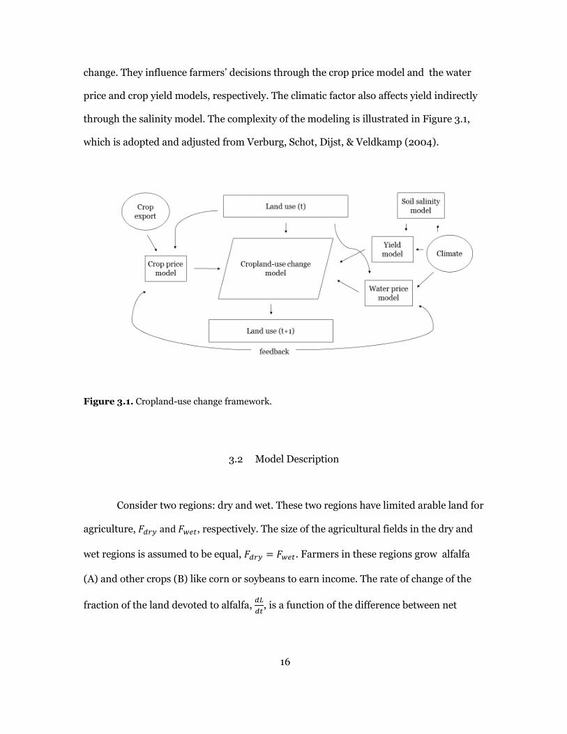
change. They influence farmers’ decisions through the crop price model and the water
price and crop yield models, respectively. The climatic factor also affects yield indirectly
through the salinity model. The complexity of the modeling is illustrated in Figure 3.1,
which is adopted and adjusted from Verburg, Schot, Dijst, & Veldkamp (2004).
Figure 3.1. Cropland-use change framework.
3.2 Model Description
Consider two regions: dry and wet. These two regions have limited arable land for
agriculture, 𝐹𝑑𝑟𝑦 and 𝐹𝑤𝑒𝑡, respectively. The size of the agricultural fields in the dry and
wet regions is assumed to be equal, 𝐹𝑑𝑟𝑦 = 𝐹𝑤𝑒𝑡. Farmers in these regions grow alfalfa
(A) and other crops (B) like corn or soybeans to earn income. The rate of change of the
fraction of the land devoted to alfalfa, 𝑑𝐿
𝑑𝑡, is a function of the difference between net
17
revenues that farmers receive from growing A and B, on a per acre basis. The equation is
given below.
𝑑𝐿
𝑑𝑡= 𝑟𝐿(1 − 𝐿)[(𝑃𝐴𝑌𝐴 − 𝐶𝐴) − (𝑃𝐵𝑌𝐵 − 𝐶𝐵)]
where 𝐿 is a fraction of the land devoted to alfalfa;
𝑡 and 𝑟 denote a time variable and a time-adjusting parameter, respectively;
𝐿(1 − 𝐿) represents a stabilizing factor that constraints a range of change;
𝑃𝐴 and 𝑃𝐵 are prices per ton of alfalfa and other crops (dollars/ton), respectively;
𝑌𝐴 and 𝑌𝐵 are average annual yields per acre of alfalfa and other crops (tons/acre),
respectively;
𝐶𝐴 and 𝐶𝐵 are costs per acre of growing two crops respectively, measured in dollars
(dollars/acre).
A positive value of 𝑑𝐿
𝑑𝑡 represents the amount of land originally devoted to other
crops, but converted to growing alfalfa in the next year; a negative value means the
opposite.
Price function (𝑷)
Price of an agricultural commodity is assumed to be determined by the quantities
demanded and supplied of the market. As the quantity demanded increases, price
increases (i.e., ↑D → ↑P); as the quantity supplied increases, price decreases (i.e., ↑S →
↓P).
𝑃 = 𝜇𝐷𝑏1𝑆𝑏2
𝜇 is the price coefficient for a specific agricultural crop;
𝐷 is the quantity demanded of the crop;
18
𝑆 is the quantity supplied of the crop;
𝑏1 is demand elasticity of a crop price, the degree of responsiveness of the crop price to a
change in the quantity demanded of the crop (𝑏1 > 0);
and 𝑏2 is supply elasticity of a crop price, the degree of responsiveness of the crop price
to a change in the quantity supplied of the crop (𝑏2 < 0).
In this model, for simplicity’s sake, it is assumed that the demand elasticity of
price is identical to the supply elasticity of price, regardless of the type of a crop (i.e.,
𝑏1 = −𝑏2 = 𝑏).
𝑃 = 𝜇 (𝐷
𝑆)
𝑏
So the price becomes a function of the relative quantity (or quantity ratio) of demand
and supply.
Quantity supplied (𝑆) of a crop is the total amount of the crop that farmers
produce and sell in the market. Because there are no agricultural imports from foreign
countries, it is obtained by summing the quantities supplied by all farmers in both the
dry and wet regions. The quantity supplied of each crop is:
𝑆𝐴 = 𝐹𝑑𝑟𝑦𝐿𝑑𝑟𝑦𝑌𝐴,𝑑𝑟𝑦 + 𝐹𝑤𝑒𝑡𝐿𝑤𝑒𝑡𝑌𝐴,𝑤𝑒𝑡
𝑆𝐵 = 𝐹𝑑𝑟𝑦(1 − 𝐿𝑑𝑟𝑦)𝑌𝐵,𝑑𝑟𝑦 + 𝐹𝑤𝑒𝑡(1 − 𝐿𝑤𝑒𝑡)𝑌𝐵,𝑤𝑒𝑡
where the type of crop is denoted by subscripts 𝐴 and 𝐵, while the type of region is
denoted by subscripts 𝑑𝑟𝑦 and 𝑤𝑒𝑡
19
Analogous to quantity supplied, quantity demanded (𝐷) of a crop is the total
amount of the crop that consumers, directly and indirectly, purchase in the regional and
international markets:
𝐷 = 𝐷(𝑅) + 𝐷(𝐼)
where 𝐷(𝑅) and 𝐷(𝐼) are the regional and international quantities demanded of the crops,
respectively. Please note that international demands are factored into the model by
assuming net exports of the crops.
Because milk production depends on the quantity and quality of feed (i.e., alfalfa
hay) that dairy cows consume, the regional quantity of alfalfa demanded (𝐷𝐴(𝑅)
) is derived
from the demand for dairy products. This is supported by Glennon (2009) who mentions
that alfalfa is directly used to produce milk in the dairy industry. Here, it is implicitly
assumed that 1) the dairy industry is the only consumer of alfalfa, and 2) dairy cows are
fed on alfalfa hay alone. In short, the demand for alfalfa is estimated by dividing the
demand for milk by alfalfa productivity of producing milk. Alfalfa productivity of
producing milk equals milk cows’ efficiency of converting alfalfa into milk.
In order to estimate regional demands for each crop, it is assumed that there are
only two agricultural goods that people can choose to buy for their food consumption:
other crops (B) and dairy products (C) (certainly, not alfalfa). People acquire utility from
consuming a particular set of those two goods. Through utility maximization under a
budget constraint, I derive Marshallian regional demand functions of the two goods.
People’s preferences are represented in utility functions. Assuming that dairy products
and other crops are independent goods, I use the Cobb-Douglas utility function. This
indicates that quantity demanded of each good depends only on the price of that good,
and not on the price of the other good.
20
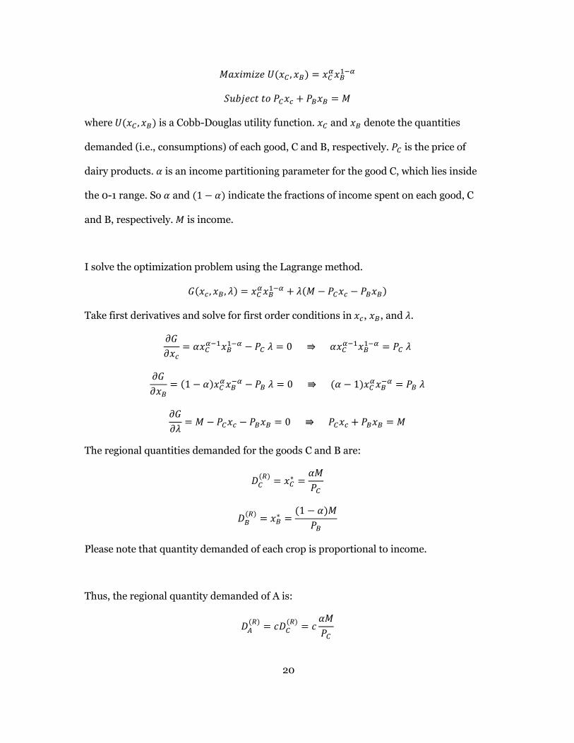
𝑀𝑎𝑥𝑖𝑚𝑖𝑧𝑒 𝑈(𝑥𝐶 , 𝑥𝐵) = 𝑥𝐶𝛼𝑥𝐵
1−𝛼
𝑆𝑢𝑏𝑗𝑒𝑐𝑡 𝑡𝑜 𝑃𝐶𝑥𝑐 + 𝑃𝐵𝑥𝐵 = 𝑀
where 𝑈(𝑥𝐶 , 𝑥𝐵) is a Cobb-Douglas utility function. 𝑥𝐶 and 𝑥𝐵 denote the quantities
demanded (i.e., consumptions) of each good, C and B, respectively. 𝑃𝐶 is the price of
dairy products. 𝛼 is an income partitioning parameter for the good C, which lies inside
the 0-1 range. So 𝛼 and (1 − 𝛼) indicate the fractions of income spent on each good, C
and B, respectively. 𝑀 is income.
I solve the optimization problem using the Lagrange method.
𝐺(𝑥𝑐 , 𝑥𝐵, 𝜆) = 𝑥𝐶𝛼𝑥𝐵
1−𝛼 + 𝜆(𝑀 − 𝑃𝐶𝑥𝑐 − 𝑃𝐵𝑥𝐵)
Take first derivatives and solve for first order conditions in 𝑥𝑐, 𝑥𝐵, and 𝜆.
𝜕𝐺
𝜕𝑥𝑐= 𝛼𝑥𝐶
𝛼−1𝑥𝐵1−𝛼 − 𝑃𝐶 𝜆 = 0 ⇛ 𝛼𝑥𝐶
𝛼−1𝑥𝐵1−𝛼 = 𝑃𝐶 𝜆
𝜕𝐺
𝜕𝑥𝐵= (1 − 𝛼)𝑥𝐶
𝛼𝑥𝐵−𝛼 − 𝑃𝐵 𝜆 = 0 ⇛ (𝛼 − 1)𝑥𝐶
𝛼𝑥𝐵−𝛼 = 𝑃𝐵 𝜆
𝜕𝐺
𝜕𝜆= 𝑀 − 𝑃𝐶𝑥𝑐 − 𝑃𝐵𝑥𝐵 = 0 ⇛ 𝑃𝐶𝑥𝑐 + 𝑃𝐵𝑥𝐵 = 𝑀
The regional quantities demanded for the goods C and B are:
𝐷𝐶(𝑅)
= 𝑥𝐶∗ =
𝛼𝑀
𝑃𝐶
𝐷𝐵(𝑅)
= 𝑥𝐵∗ =
(1 − 𝛼)𝑀
𝑃𝐵
Please note that quantity demanded of each crop is proportional to income.
Thus, the regional quantity demanded of A is:
𝐷𝐴(𝑅)
= 𝑐𝐷𝐶(𝑅)
= 𝑐𝛼𝑀
𝑃𝐶
21
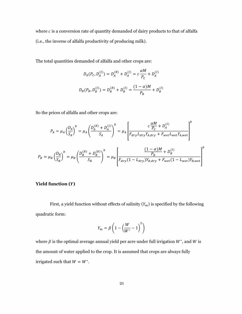
where 𝑐 is a conversion rate of quantity demanded of dairy products to that of alfalfa
(i.e., the inverse of alfalfa productivity of producing milk).
The total quantities demanded of alfalfa and other crops are:
𝐷𝐴(𝑃𝐶 , 𝐷𝐴(𝐼)
) = 𝐷𝐴(𝑅)
+ 𝐷𝐴(𝐼)
= 𝑐𝛼𝑀
𝑃𝐶+ 𝐷𝐴
(𝐼)
𝐷𝐵(𝑃𝐵, 𝐷𝐵(𝐼)
) = 𝐷𝐵(𝑅)
+ 𝐷𝐵(𝐼)
=(1 − 𝛼)𝑀
𝑃𝐵+ 𝐷𝐵
(𝐼)
So the prices of alfalfa and other crops are:
𝑃𝐴 = 𝜇𝐴 (𝐷𝐴
𝑆𝐴)
𝑏
= 𝜇𝐴 (𝐷𝐴
(𝑅)+ 𝐷𝐴
(𝐼)
𝑆𝐴)
𝑏
= 𝜇𝐴 [𝑐
𝛼𝑀𝑃𝐶
+ 𝐷𝐴(𝐼)
𝐹𝑑𝑟𝑦𝐿𝑑𝑟𝑦𝑌𝐴,𝑑𝑟𝑦 + 𝐹𝑤𝑒𝑡𝐿𝑤𝑒𝑡𝑌𝐴,𝑤𝑒𝑡]
𝑏
𝑃𝐵 = 𝜇𝐵 (𝐷𝐵
𝑆𝐵)
𝑏
= 𝜇𝐵 (𝐷𝐵
(𝑅)+ 𝐷𝐵
(𝑅)
𝑆𝐵)
𝑏
= 𝜇𝐵 [
(1 − 𝛼)𝑀𝑃𝐵
+ 𝐷𝐵(𝐼)
𝐹𝑑𝑟𝑦(1 − 𝐿𝑑𝑟𝑦)𝑌𝐵,𝑑𝑟𝑦 + 𝐹𝑤𝑒𝑡(1 − 𝐿𝑤𝑒𝑡)𝑌𝐵,𝑤𝑒𝑡]
𝑏
Yield function (𝒀)
First, a yield function without effects of salinity (𝑌𝑚) is specified by the following
quadratic form:
𝑌𝑚 = 𝛽 (1 − (𝑊
𝑊∗− 1)
2
)
where 𝛽 is the optimal average annual yield per acre under full irrigation 𝑊∗, and 𝑊 is
the amount of water applied to the crop. It is assumed that crops are always fully
irrigated such that 𝑊 = 𝑊∗.
22
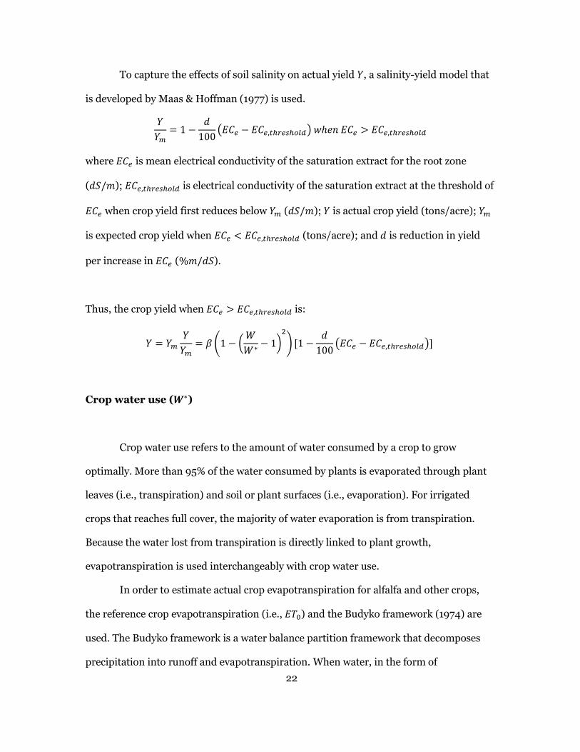
To capture the effects of soil salinity on actual yield 𝑌, a salinity-yield model that
is developed by Maas & Hoffman (1977) is used.
𝑌
𝑌𝑚= 1 −
𝑑
100(𝐸𝐶𝑒 − 𝐸𝐶𝑒,𝑡ℎ𝑟𝑒𝑠ℎ𝑜𝑙𝑑) 𝑤ℎ𝑒𝑛 𝐸𝐶𝑒 > 𝐸𝐶𝑒,𝑡ℎ𝑟𝑒𝑠ℎ𝑜𝑙𝑑
where 𝐸𝐶𝑒 is mean electrical conductivity of the saturation extract for the root zone
(𝑑𝑆/𝑚); 𝐸𝐶𝑒,𝑡ℎ𝑟𝑒𝑠ℎ𝑜𝑙𝑑 is electrical conductivity of the saturation extract at the threshold of
𝐸𝐶𝑒 when crop yield first reduces below 𝑌𝑚 (𝑑𝑆/𝑚); 𝑌 is actual crop yield (tons/acre); 𝑌𝑚
is expected crop yield when 𝐸𝐶𝑒 < 𝐸𝐶𝑒,𝑡ℎ𝑟𝑒𝑠ℎ𝑜𝑙𝑑 (tons/acre); and 𝑑 is reduction in yield
per increase in 𝐸𝐶𝑒 (%𝑚/𝑑𝑆).
Thus, the crop yield when 𝐸𝐶𝑒 > 𝐸𝐶𝑒,𝑡ℎ𝑟𝑒𝑠ℎ𝑜𝑙𝑑 is:
𝑌 = 𝑌𝑚
𝑌
𝑌𝑚= 𝛽 (1 − (
𝑊
𝑊∗− 1)
2
) [1 −𝑑
100(𝐸𝐶𝑒 − 𝐸𝐶𝑒,𝑡ℎ𝑟𝑒𝑠ℎ𝑜𝑙𝑑)]
Crop water use (𝑾∗)
Crop water use refers to the amount of water consumed by a crop to grow
optimally. More than 95% of the water consumed by plants is evaporated through plant
leaves (i.e., transpiration) and soil or plant surfaces (i.e., evaporation). For irrigated
crops that reaches full cover, the majority of water evaporation is from transpiration.
Because the water lost from transpiration is directly linked to plant growth,
evapotranspiration is used interchangeably with crop water use.
In order to estimate actual crop evapotranspiration for alfalfa and other crops,
the reference crop evapotranspiration (i.e., 𝐸𝑇0) and the Budyko framework (1974) are
used. The Budyko framework is a water balance partition framework that decomposes
precipitation into runoff and evapotranspiration. When water, in the form of
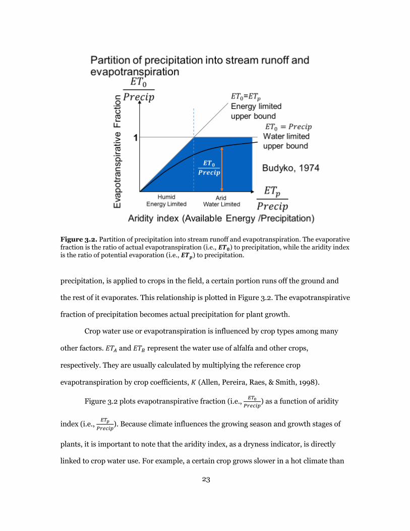
23
precipitation, is applied to crops in the field, a certain portion runs off the ground and
the rest of it evaporates. This relationship is plotted in Figure 3.2. The evapotranspirative
fraction of precipitation becomes actual precipitation for plant growth.
Crop water use or evapotranspiration is influenced by crop types among many
other factors. 𝐸𝑇𝐴 and 𝐸𝑇𝐵 represent the water use of alfalfa and other crops,
respectively. They are usually calculated by multiplying the reference crop
evapotranspiration by crop coefficients, 𝐾 (Allen, Pereira, Raes, & Smith, 1998).
Figure 3.2 plots evapotranspirative fraction (i.e., 𝐸𝑇0
𝑃𝑟𝑒𝑐𝑖𝑝) as a function of aridity
index (i.e., 𝐸𝑇𝑝
𝑃𝑟𝑒𝑐𝑖𝑝). Because climate influences the growing season and growth stages of
plants, it is important to note that the aridity index, as a dryness indicator, is directly
linked to crop water use. For example, a certain crop grows slower in a hot climate than
Figure 3.2. Partition of precipitation into stream runoff and evapotranspiration. The evaporative fraction is the ratio of actual evapotranspiration (i.e., 𝑬𝑻𝟎) to precipitation, while the aridity index is the ratio of potential evaporation (i.e., 𝑬𝑻𝒑) to precipitation.
24
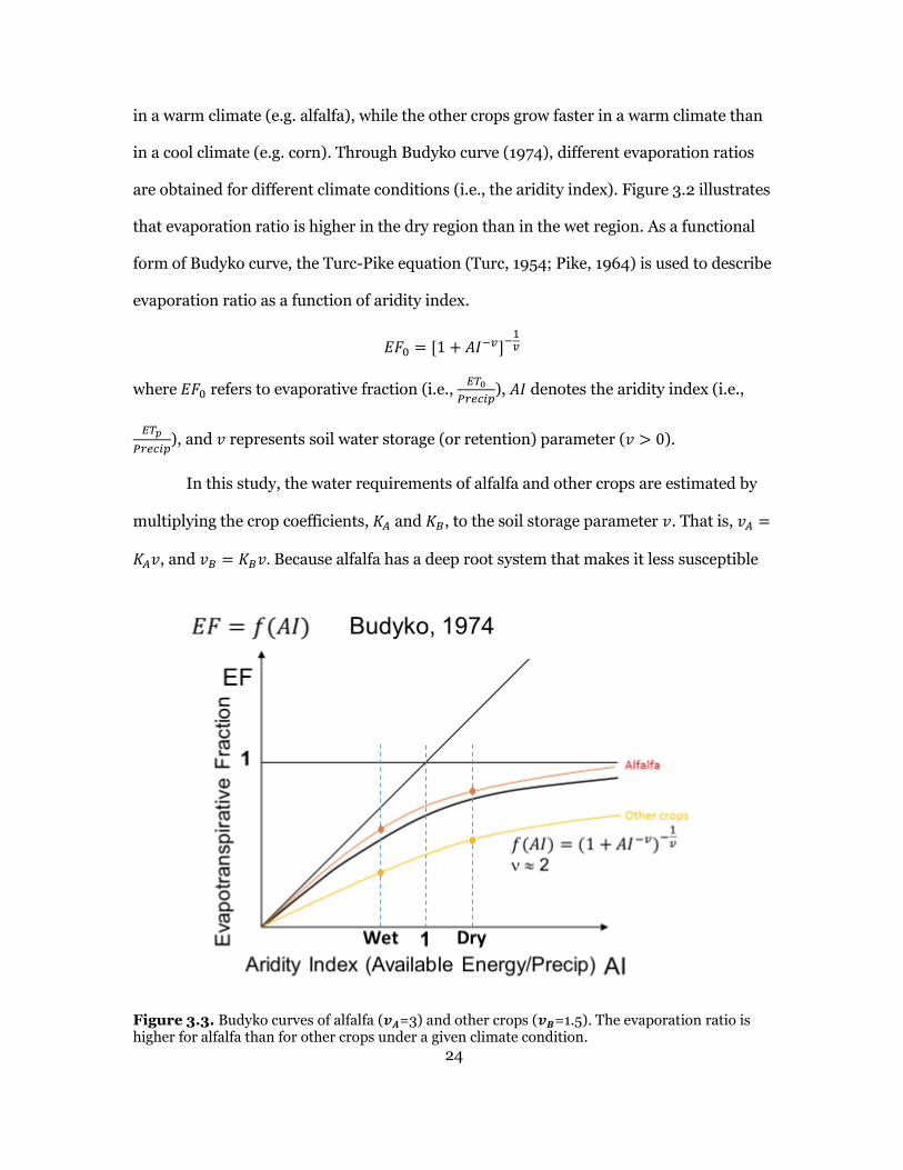
in a warm climate (e.g. alfalfa), while the other crops grow faster in a warm climate than
in a cool climate (e.g. corn). Through Budyko curve (1974), different evaporation ratios
are obtained for different climate conditions (i.e., the aridity index). Figure 3.2 illustrates
that evaporation ratio is higher in the dry region than in the wet region. As a functional
form of Budyko curve, the Turc-Pike equation (Turc, 1954; Pike, 1964) is used to describe
evaporation ratio as a function of aridity index.
𝐸𝐹0 = [1 + 𝐴𝐼−𝑣]−1𝑣
where 𝐸𝐹0 refers to evaporative fraction (i.e., 𝐸𝑇0
𝑃𝑟𝑒𝑐𝑖𝑝), 𝐴𝐼 denotes the aridity index (i.e.,
𝐸𝑇𝑝
𝑃𝑟𝑒𝑐𝑖𝑝), and 𝑣 represents soil water storage (or retention) parameter (𝑣 > 0).
In this study, the water requirements of alfalfa and other crops are estimated by
multiplying the crop coefficients, 𝐾𝐴 and 𝐾𝐵, to the soil storage parameter 𝑣. That is, 𝑣𝐴 =
𝐾𝐴𝑣, and 𝑣𝐵 = 𝐾𝐵𝑣. Because alfalfa has a deep root system that makes it less susceptible
Figure 3.3. Budyko curves of alfalfa (𝒗𝑨=3) and other crops (𝒗𝑩=1.5). The evaporation ratio is higher for alfalfa than for other crops under a given climate condition.
25
to water stress during dry periods, 𝐾𝐴 is assumed to be greater than 𝐾𝐵, and therefore
𝑣𝐴 > 𝑣𝐵. Graphically, the crop coefficients shift the Budyko curve close to or away from
the water and energy limited upper bounds, making it a plant-specific Budyko curve (see
Figure 3.3).
Crop water uses per acre for A and B, 𝑊𝐴∗ and 𝑊𝐵
∗, are calculated by multiplying
the optimal yield by their virtual water content. Virtual water content represents the
volume of water used to produce a unit of crop yield.
𝑊𝐴∗ = 𝑌𝐴𝑉𝑊𝐶𝐴
𝑊𝐵∗ = 𝑌𝐵𝑉𝑊𝐶𝐵
where 𝑉𝑊𝐶𝐴 and 𝑉𝑊𝐶𝐵 are virtual water contents of alfalfa and other crops, respectively
(𝑚3/ton); 𝑌𝐴 and 𝑌𝐵 are yields of alfalfa and other crops, respectively (tons/acre).
Precipitation and irrigation water are the two main sources of crop water use.
Particularly, in the dry region, irrigation is necessary to supplement insufficient rainfall.
The irrigation water requirement, 𝐼𝑟𝑟𝑖, can be derived by subtracting actual
precipitation, 𝑃𝑟𝑒𝑐𝑖𝑝 × 𝐸𝐹, from crop water requirement, 𝑊∗.
𝑊∗ = 𝑃𝑟𝑒𝑐𝑖𝑝 × 𝐸𝐹 + 𝐼𝑟𝑟𝑖
𝐼𝑟𝑟𝑖 = 𝑊∗ − 𝑃𝑟𝑒𝑐𝑖𝑝 × 𝐸𝐹
where 𝑃𝑟𝑒𝑐𝑖𝑝 and 𝐼𝑟𝑟𝑖 denote the amounts of precipitation and irrigation water per acre
(𝑚3/acre).
So the irrigation water requirements are:
𝐼𝑟𝑟𝑖𝐴 = 𝑊𝐴∗ − 𝑃𝑟𝑒𝑐𝑖𝑝 × 𝐸𝐹𝐴
𝐼𝑟𝑟𝑖𝐵 = 𝑊𝐵∗ − 𝑃𝑟𝑒𝑐𝑖𝑝 × 𝐸𝐹𝐵
26
Cost function (𝑪)
The cost function primarily consists of irrigation water costs and labor costs, and
a cost of land is implicitly embodied in the model setup even though land is not a
limiting factor in the model.
𝐶 = 𝑃𝑊 × 𝐼𝑟𝑟𝑖 + 𝑃𝑈 × 𝑈 + 𝐸 = 𝑃𝑊 × (𝑊∗ − 𝑃𝑟𝑒𝑐𝑖𝑝 × 𝐸𝐹) + 𝑃𝑈 × 𝑈 + 𝐸
where 𝑃𝑊 is the price of water (dollars/𝑚3); 𝑃𝑈 is hourly wage rate(dollars/hour); 𝑈 is
average labor hours per acre needed to grow crops (hours/acre); and 𝐸 is a crop-specific
extra lump sum cost (dollars/acre).
Analogous to crop prices, the water price is specified as a function of relative ratio
between available water supplies and current water demands.. However, the water rates
are not assumed to be equal between the dry and wet regions to reflect the different
water situation in each region. Water demands in the dry and wet regions correspond to
the total amount of water needed for irrigating alfalfa and other crops in each region.
The aridity index is assumed to determine the short-term water supply. Then, the
functional form of water rates in each region is specified as:
𝑃𝑊 = 𝜋 [exp (𝑊𝑎𝑡𝑒𝑟 𝑑𝑒𝑚𝑎𝑛𝑑
𝑊𝑎𝑡𝑒𝑟 𝑠𝑢𝑝𝑝𝑙𝑦) − 1]
= 𝜋 [exp (𝐹[𝐿(𝑊𝐴
∗ − 𝑃𝑟𝑒𝑐𝑖𝑝 ∙ 𝐸𝐹𝐴) + (1 − 𝐿)(𝑊𝐵∗ − 𝑃𝑟𝑒𝑐𝑖𝑝 ∙ 𝐸𝐹𝐵)]
1010 ∙ 0.5𝐴𝐼 ) − 1]
where 𝜋 is a decelerating parameter.
27
CHAPTER 4
RESULTS
In this chapter, I first develop a baseline scenario to which other scenarios are
compared. The three scenarios are then described. Then I explore a range of parameters
in each of the three scenarios to address the research questions posed. The model with
default parameter values illustrates the baseline projections for alfalfa acreage changes
in the dry and wet regions for the next hundred years. To validate the baseline model, I
use the current trend in cropland-use change.
Time Frame
The model uses an annual time scale from year zero to year 100 in the
calculations. The land-use change decisions are made on a yearly basis as farmers
usually schedule their farming activities based on the information from the previous year
(e.g., lagged prices) and one year is naturally suitable for a growing season for most of
crops. In this context, short-term decisions like monthly cropping of alfalfa are assumed
to aggregate to annual changes.
Alfalfa acreage changes
Crop areas are expressed as fractions of the total land area devoted to each crop
within each region. Because the amount of agricultural land is assumed to be the same
28
across the regions, fractions of cropland devoted to certain crops can be interpreted as
land areas devoted to those crops in absolute terms. It is only a matter of scaling.
4.1 Baseline Model
The cropland area devoted to alfalfa has steadily diminished from 1993 to 2013 in
the United States. In the last two decades, it has decreased by nearly 6.8 million acres
throughout the western and eastern US as a whole. In the east, the amount of land
devoted to alfalfa has declined by about 31.5% in the last decade, while it has dropped by
about 9.5% in the west for the same time period (see Figure 1.5). These figures show that
alfalfa is more quickly fading out of rain-fed areas (i.e., the midwestern and eastern US)
0 20 40 60 80 1000
0.05
0.1
0.15
0.2
0.25
Time
Ld, L
w
0 20 40 60 80 100150
200
250
300
Time
Pa, P
b
0.16 0.18 0.2 0.220
0.01
0.02
0.03
0.04
Ld
Lw
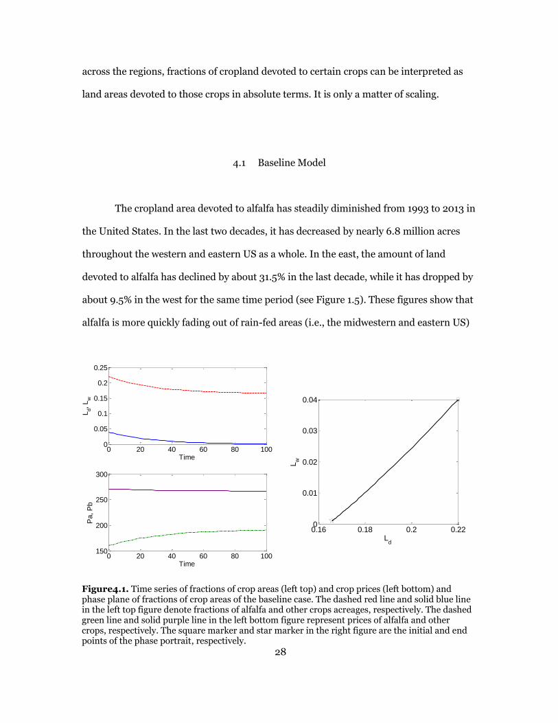
Figure4.1. Time series of fractions of crop areas (left top) and crop prices (left bottom) and phase plane of fractions of crop areas of the baseline case. The dashed red line and solid blue line in the left top figure denote fractions of alfalfa and other crops acreages, respectively. The dashed green line and solid purple line in the left bottom figure represent prices of alfalfa and other crops, respectively. The square marker and star marker in the right figure are the initial and end points of the phase portrait, respectively.
29
than in dry areas (i.e., the western US). However, due to pressure for land-use change for
urbanization and other profitable crops, the overall trend of both regions is the decline of
alfalfa acreages. As of 2013, the fractions of acreage planted with alfalfa to the total
principle crops acreage are approximately 21.8% and 4% for the western and non-
western US, respectively. These numbers were used as default values of the initial alfalfa
acreage fractions for the dry and wet regions in the model. That is, 𝐿𝑑𝑟𝑦(0) = 0.22 and
𝐿𝑤𝑒𝑡(0) = 0.04.
The top-left panel of Figure 4.1 shows the time series of percentage changes of
alfalfa acreage in the dry and wet regions. Under the baseline assumptions, the model
predicts that percentages of alfalfa acreages will decrease constantly in both regions,
with the rapid rate of change for the wet region compared to the dry region (see Figure
4.1). Therefore, the results from the baseline scenario are consistent with the overall
trend of alfalfa acreage changes.
Prices of alfalfa and other crops
Depending on conditions at a given location, crop prices vary widely across
regions. However, I invoke the law of one price for simplicity and clarity in result
interpretation. In other words, there is only one price of alfalfa or other crops throughout
the dry and wet regions.
As the supply of alfalfa becomes tighter as a result of the overall decrease in
alfalfa acreages, the average annual price of alfalfa hay almost doubled from $102.5 per
ton in 2005 to $205.8 per ton in 2013. On the demand side, the rise in alfalfa price is
partly due to the rapid increase in alfalfa hay exports to foreign countries, including the
United Arab Emirates and China, over the past 5 years since 2007. The bottom-left panel
30
of Figure 4.1 shows that alfalfa hay prices steadily increase as fractions of cropland
devoted to alfalfa decline in both regions. Thus, the model prediction of alfalfa price is
compatible with the current rising trend of alfalfa prices. For prices of other crops, I refer
to the future USDA’s projections for corn and soybean prices.
4.2 Three Scenarios
First Scenario: International demands for alfalfa continue to grow (or at least stay
high).
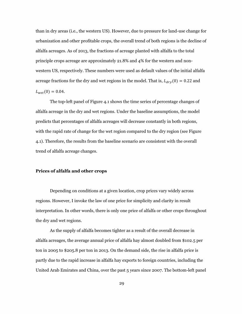
According to Putnam, Mathews, & Sumner (2013), the percentage of alfalfa hay
exports has increased from 1.5% in 2007 to 4.3% in 2012, while the percentage of exports
of alfalfa hay grown in western states has soared from 5% in 2007 to 12.5% in 2012.
748,505
1,973,748
0
500,000
1,000,000
1,500,000
2,000,000
2,500,000
2007 2008 2009 2010 2011 2012 2013
Volume of Alfalfa Hay Exports (MT)
Figure 4.2. Alfalfa hay exports from 2007 to 2013. (Source: Foreign Agricultural Service U.S. Trade)
31
Figure 4.2 shows that the volume of alfalfa hay exported has more than doubled in the
2007-2013 period from 0.7 million metric tons in 2007 to 1.9 million metric tons in
2013. While Japan and Korea have been the regular major importers of US alfalfa hay,
this rapid increase is mainly due to the United Arab Emirates and China. The United
Arab Emirates imported 27,946 metric tons of alfalfa hay in 2007 and increased more
than 23 times to 661,569 metric tons in 2013. China’s alfalfa hay imports have increased
about 250 times from 2,321 metric tons in 2007 to 576,652 metric tons in 2012.
Although there are many factors that make it difficult to accurately predict the
future international market demands for alfalfa hay, it is anticipated that overseas
demands for alfalfa will grow due to increasing demand for dairy products and scarce
land and water resources in the Middle East and Asia (Fuller, Huang, Ma, & Rozelle,
2006; Putnam et al., 2013). In the simulation, alfalfa hay exports are increased 2 times, 5
times, and 10 times compared to the baseline scenario to see how increasing overseas
demand for alfalfa will impact the distribution of crop production across the dry and wet
regions.
Second Scenario: Deficit irrigation is widely imposed in the water-scarce dry region.
Alfalfa is a “good candidate for deficit irrigation” because it is well adapted to dry
climates (i.e., drought resistant) as discussed in the introductory chapter and has the
ability to go dormant when crop water use or evapotranspiration cannot be fully satisfied
(Bauder et al., 2011). Furthermore, because alfalfa is a cool season crop, it “grows slowly
and blooms quickly” during the hot and dry summer, which reduces both the quantity
and quality of alfalfa harvested (Glennon, 2009). For this reason, turning irrigation of
alfalfa fields off during midsummer (usually July and August) seems a reasonable choice
32
under limited water situations. In short, due to these characteristics, alfalfa can be deficit
irrigated to conserve water under severe water stress, freeing up water for other
purposes.
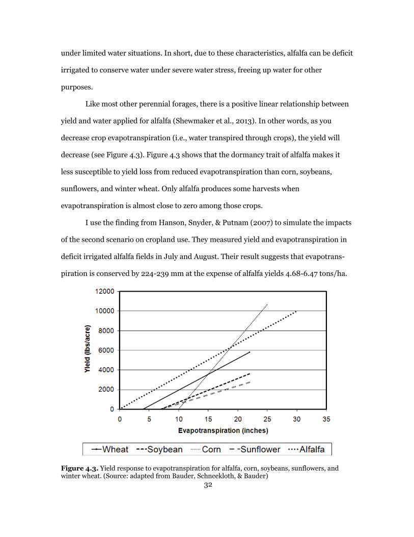
Like most other perennial forages, there is a positive linear relationship between
yield and water applied for alfalfa (Shewmaker et al., 2013). In other words, as you
decrease crop evapotranspiration (i.e., water transpired through crops), the yield will
decrease (see Figure 4.3). Figure 4.3 shows that the dormancy trait of alfalfa makes it
less susceptible to yield loss from reduced evapotranspiration than corn, soybeans,
sunflowers, and winter wheat. Only alfalfa produces some harvests when
evapotranspiration is almost close to zero among those crops.
I use the finding from Hanson, Snyder, & Putnam (2007) to simulate the impacts
of the second scenario on cropland use. They measured yield and evapotranspiration in
deficit irrigated alfalfa fields in July and August. Their result suggests that evapotrans-
piration is conserved by 224-239 mm at the expense of alfalfa yields 4.68-6.47 tons/ha.
Figure 4.3. Yield response to evapotranspiration for alfalfa, corn, soybeans, sunflowers, and winter wheat. (Source: adapted from Bauder, Schneekloth, & Bauder)
33
Third Scenario: Long-term droughts persist or intensify, leading to reduced
precipitation.
According to Maliva & Missimer (2012), drought refers to a “temporary,
recurring reduction in the precipitation” at a given place in a broad sense. Because
aridity is a long-term climate condition, both the dry and wet regions have drought
periods. However, due to the higher variation in precipitation in dry regions, dry regions
are more vulnerable to droughts than wet regions, causing severe consequences in the
dry regions.
Drought is one of the major reasons for water scarcity in the dry regions. To
investigate how farmers cope with the water-limited situation, I reduce the precipitation
of the dry region by 2 inch, 5 inch, and 10 inch compared to the baseline scenario.
4.3 Simulation Results
First scenario results:
0.12 0.13 0.14 0.15 0.16 0.17 0.18 0.19 0.2 0.21 0.220.005
0.01
0.015
0.02
0.025
0.03
0.035
0.04
Ld
Lw
Phase portraits of different levels of international demands
0.35 times (2007)
baseline (2013)
2 times
5 times
10 times
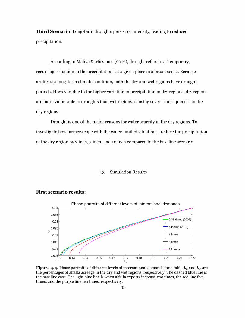
Figure 4.4. Phase portraits of different levels of international demands for alfalfa. 𝑳𝒅 and 𝑳𝒘 are the percentages of alfalfa acreage in the dry and wet regions, respectively. The dashed blue line is the baseline case. The light blue line is when alfalfa exports increase two times, the red line five times, and the purple line ten times, respectively.
34
The increase in alfalfa exports slows down the rate of reduction in the percentage
of alfalfa acreage in the dry region. The percentage of land devoted to alfalfa at the end
point is 13.5% for the ten times increase in international demand for alfalfa, while it is
12% for the baseline scenario. For the wet region, there is not much difference shown in
the cropland percentage change.
Second scenario results:
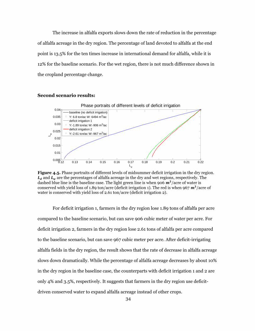
For deficit irrigation 1, farmers in the dry region lose 1.89 tons of alfalfa per acre
compared to the baseline scenario, but can save 906 cubic meter of water per acre. For
deficit irrigation 2, farmers in the dry region lose 2.61 tons of alfalfa per acre compared
to the baseline scenario, but can save 967 cubic meter per acre. After deficit-irrigating
alfalfa fields in the dry region, the result shows that the rate of decrease in alfalfa acreage
slows down dramatically. While the percentage of alfalfa acreage decreases by about 10%
in the dry region in the baseline case, the counterparts with deficit irrigation 1 and 2 are
only 4% and 3.5%, respectively. It suggests that farmers in the dry region use deficit-
driven conserved water to expand alfalfa acreage instead of other crops.
0.12 0.13 0.14 0.15 0.16 0.17 0.18 0.19 0.2 0.21 0.220.005
0.01
0.015
0.02
0.025
0.03
0.035
0.04
Ld
Lw
Phase portraits of different levels of deficit irrigation
baseline (no deficit irrigation)
Y: 6.8 ton/ac W: 6494 m3/ac
deficit irrigation 1
Y:-1.89 ton/ac W:-906 m3/ac
deficit irrigation 2
Y:-2.61 ton/ac W:-967 m3/ac
Figure 4.5. Phase portraits of different levels of midsummer deficit irrigation in the dry region. 𝑳𝒅 and 𝑳𝒘 are the percentages of alfalfa acreage in the dry and wet regions, respectively. The
dashed blue line is the baseline case. The light green line is when 906 𝒎𝟑/acre of water is conserved with yield loss of 1.89 ton/acre (deficit irrigation 1). The red is when 967 𝒎𝟑/acre of water is conserved with yield loss of 2.61 ton/acre (deficit irrigation 2).
35
Third scenario results:
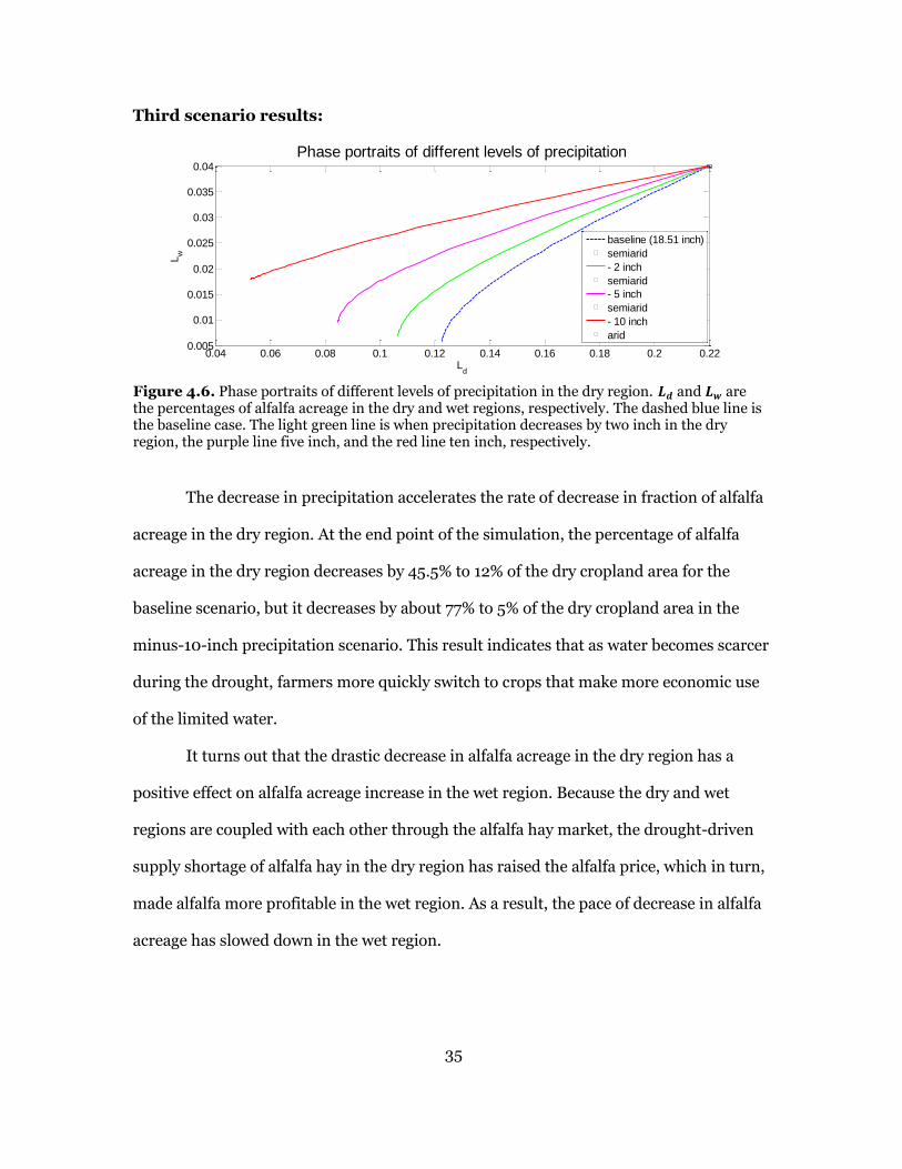
The decrease in precipitation accelerates the rate of decrease in fraction of alfalfa
acreage in the dry region. At the end point of the simulation, the percentage of alfalfa
acreage in the dry region decreases by 45.5% to 12% of the dry cropland area for the
baseline scenario, but it decreases by about 77% to 5% of the dry cropland area in the
minus-10-inch precipitation scenario. This result indicates that as water becomes scarcer
during the drought, farmers more quickly switch to crops that make more economic use
of the limited water.
It turns out that the drastic decrease in alfalfa acreage in the dry region has a
positive effect on alfalfa acreage increase in the wet region. Because the dry and wet
regions are coupled with each other through the alfalfa hay market, the drought-driven
supply shortage of alfalfa hay in the dry region has raised the alfalfa price, which in turn,
made alfalfa more profitable in the wet region. As a result, the pace of decrease in alfalfa
acreage has slowed down in the wet region.
0.04 0.06 0.08 0.1 0.12 0.14 0.16 0.18 0.2 0.220.005
0.01
0.015
0.02
0.025
0.03
0.035
0.04
Ld
Lw
Phase portraits of different levels of precipitation
baseline (18.51 inch)
semiarid
- 2 inch
semiarid
- 5 inch
semiarid
- 10 inch
arid
Figure 4.6. Phase portraits of different levels of precipitation in the dry region. 𝑳𝒅 and 𝑳𝒘 are the percentages of alfalfa acreage in the dry and wet regions, respectively. The dashed blue line is the baseline case. The light green line is when precipitation decreases by two inch in the dry region, the purple line five inch, and the red line ten inch, respectively.
36
CHAPTER 5
CONCLUSIONS AND DISCUSSION
Land and water are the limited resources that are fundamentally essential to
meet our demands for food, housing, and other basic necessities. In this study, I
investigated the different pathways of cropland development under different water
situations. By simplifying the United States into a binary world of the arid West and the
humid East, the impact of water scarcity on crop production was clearly exposed. The
results of this study suggest that 1) in order to cope with the water limited situation,
farmers will shift to less water-intensive crops that hold higher economic values and 2)
in drought years, farmers can deficit-irrigate their alfalfa fields, leaving more water to be
used for other purposes. The first finding implies that when water is scarce, the limited
land will be used for the purpose of creating higher values with less water. This further
implies that, if the scope of the study is not restricted only to agriculture, removing
agricultural fields from production and converting the land and conserved water to
urban and industrial sectors would be the most likely future. The second finding implies
that without the removal of agricultural land from production, there could be multiple
ways of meeting (or alleviating) water demands from various sectors. Apart from deficit
irrigation, farmers might be able to continue farming by increasing irrigation efficiency,
e.g., switching from gravity irrigation to micro-irrigation. Also, the model results
generally suggest that alfalfa production gradually shifted out of wet regions into arid
regions under the three scenarios. This implies that the limited western irrigation water
37
used to grow alfalfa is the price for the consumption of dairy products such as milk,
cheese, butter, ice cream, and yogurt.
Results from the cropland-use change model in this study are fundamentally
driven by relative advantages that alternative crops have over alfalfa in terms of cash
value and crop water use. For this reason, every scenario in this study shows a general
trend of decline in alfalfa acreage (or rise in alternative crop acreage) in both the dry and
wet region. It explains why the model generally predicts long-term outcomes where the
fraction of alfalfa acreage in the wet region goes to zero and the equivalent of the dry
region goes to some point below the original point over the study period. The fraction of
land devoted to alfalfa in the dry region does not go up until the system has an extreme
demand for alfalfa. This finding suggests that a combination of rise in dairy demand and
growing water shortages around the world could eventually lead to the expansion of
alfalfa acreage in a region like the western US.
There is great uncertainty regarding how global climate change will affect
regional weather conditions. That said, it is highly probable that arid and semiarid
regions will experience more frequent and prolonged droughts in the future. As
demonstrated in the third scenario, the fraction of land devoted to alfalfa (or the total
alfalfa acreage) in a region can be used, in conjunction with other trends, as a signal of
aggravated water scarcity or competition for water in the region. Moreover, the model
shows that with extended droughts, the alfalfa acreage decrease in the wet region is
suppressed to some extent. Theoretically, this provides an opportunity for virtual water
transfer from wet regions to dry regions, which makes sense in terms of water use
efficiency.
As the US is often seen as a microcosm of a variety of climate regions in the
world, the model developed in this study may be generalized to represent the dry and wet
38
parts of the world and their land-use change. Regardless of whether water is scarce or
not, in order to sustain the population and regional economies, every climate region is
required to produce food, which relies on freshwater resources. That is, either self-
growing or exporting regions have to pay the price for land and water to provide food.
Water-stressed arid regions (e.g., the Middle East and some parts of Asia) strategically
seek to supplement local water deficit through the import of forage crops like alfalfa from
other regions. In recompense for export proceeds, these exporting regions (e.g., the arid
western US) should bear the cost of water for crop production. Therefore, the increase in
alfalfa exports shown in the first scenario reflects not only newly available economic
opportunities for local farmers in exporting regions, but also the changing land and
water situations among arid and wet regions in the world. As a globalized commodity,
alfalfa—as well as other water-intensive, low-value crops—may potentially be used, in
conjunction with other factors, to study patterns of how much we pay for food security in
regards with the limited water and how this payment changes around the world over
time.
This stylized model involves a number of simplifying assumptions with an aim for
clarity in result interpretation. However, as typical in such a model, its caveats and
limitations must be properly recognized. For example, crop prices and fractions of land
devoted to crops are based on 2013 levels, which have been influenced by a special
period that includes the 2007-2008 world food and global finance crises. In that period,
major world crop prices soared, including alfalfa, and housing prices plummeted in the
aftermath of the financial crisis. In the following recession, the pressure for land use was
lessened and crop price rises provided economic opportunities for farmers (usually
large-scale farmers who have access to farm loan); the combination of these two events
decelerated land-use change from agriculture to urban uses. Such unusual historical
39
events can have lasting impacts on land use. Therefore, explicitly incorporating these
types of events into the model can significantly alter the results.
Another important caveat is that the model assumes homogeneity in alfalfa
production processes within each region. This masks significant regional heterogeneity
in reality. Discrepancies in climate, soil types, water availability, regional markets, and
transportation costs within the dry and wet regions can create bias in estimating the
production of crops. In addition, by assuming fully-irrigated agricultural fields and a
uniform and flat water price structure, the model does not capture the fact that farmers
face wildly different degrees of surface water shortage and varying groundwater pumping
costs due to declining water levels. Furthermore, the model does not include temporal
fluctuations in crop prices and precipitation levels, which could also significantly change
the model results.
The water scarcity problem in arid regions will not be easy to address since it
entails a complex set of issues such as food security, increasing demand from urban and
industrial use, and uncertain climate changes. Among those issues, only some specific
aspects of the problem are addressed in this study. Taking this as a stepping stone, I have
identified several potential areas of the model extension. For example, formulating the
structure of relative advantages for selected crops differently will further our
understanding of multiple regimes in a coupled ecological-economic system of land use.
In addition, by addressing variability of prices and climate conditions, bimodal surface
water and groundwater cost structure, and heterogeneous characteristics of the climate
zones in the model, I will be able to improve the model results and gain more insights on
crop production in a water-stressed region.
40
REFERENCES
Allen, R. G., Pereira, L. S., Raes, D., & Smith, M. (1998). Crop evapotranspiration-Guidelines fo computing crop water requirements-Irrigation and drainage paper 56. Rome.
Bauder, T., Hansen, N., Lindenmeyer, B., Bauder, J., & Brummer, J. (2011). Limited
irrigation of alfalfa in the Great Plains and Intermountain West. Retrieved from http://region8water.colostate.edu/PDFs/limited_irr_alfalfa_greatplains_final.pdf
Bauder, T., Schneekloth, J., & Bauder, J. (n.d.). Principles and practices for irrigation
management with limited water. Budyko, M.I. (1974). Climate and life, Orlando, FL: Academic Press. Butler, L. J. (2010). Global economic trends: Forage, feeds, and milk. In Proceedings of
2010 California Alfalfa & Forage Symposium and Corn/Cereal Silage Mini-Symposium. Visalia, CA.
Confalonieri, R., & Bechini, L. (2004). A preliminary evaluation of the simulation model
CropSyst for alfalfa. European Journal of Agronomy, 21(2), 223–237. http://doi.org/10.1016/j.eja.2003.08.003
Culp, P. W., & Glennon, R. (2012). Parched in the West, but shipping water to China,
bale by bale. Wall Street Journal. NY. Fuller, F., Huang, J., Ma, H., & Rozelle, S. (2006). Got milk? The rapid rise of China’s
dairy sector and its future prospects. Food Policy, 31(3 SPEC. ISS.), 201–215. http://doi.org/10.1016/j.foodpol.2006.03.002
Glennon, R. (2009). Unquenchable: America’s water crisis and what to do about it.
island Press. Glennon, R., Libecap, G., & Culp, P. W. (2014). Shopping for water: How the market
can mitigate water shortages in the American West. Retrieved from http://www.brookings.edu/~/media/research/files/papers/2014/10/20 thp us water p
Hanson, B., Snyder, R., & Putnam, D. (2007). Deficit irrigation of alfalfa as a strategy for
providing water for water-short areas. Agricultural Water Management, 93, 73–78. http://doi.org/10.2495/SI080121
Hoekstra, A. Y. (2014). Water for animal products: a blind spot in water policy.
Environmental Research Letters, 9(9), 091003. http://doi.org/10.1088/1748-9326/9/9/091003
Maas, E. V., & Hoffman, G. J. (1977). Crop salt tolerance-current assessment. American
Society of Civil Engineers.
41
Maliva, R., & Missimer, T. (2012). Arid lands water evaluation and management.
Springer. http://doi.org/10.1007/978-3-642-29104-3 Martin, N. P., Mertens, D. R., & Weimer, P. J. (2004). Alfalfa: Hay, haylage, baleage, and
other novel products. In Proceedings of the Idaho Alfalfa and Forage Conference. Idaho. Retrieved from http://www.extension.uidaho.edu/forage/Proceedings/2004 Proceedings pdf/Alfalfa hay_haylage--Martin.pdf
Mubako, S. T., & Lant, C. L. (2013). Agricultural virtual water trade and water footprint
of U.S. states. Annals of the Association of American Geographers, 103(2), 385–396. http://doi.org/10.1080/00045608.2013.756267
Pike, J. G. (1964). The estimation of annual run-off from meteorological data in a
tropical climate. Journal of Hydrology, 2(2), 116–123. http://doi.org/10.1016/0022-1694(64)90022-8
Ponce, V. M., Pandey, R. P., & Ercan, S. (2000). Characterization of drought across
climatic spectrum. Journal of Hydrologic Engineering, 5(2), 222–224. Putnam, D. (2010). Evaluating the value of field crops: An environmental balance sheet
for alfalfa. In Proceedings of 2010 California Alfalfa & Forage Symposium and Corn/Cereal Silage Mini-Symposium. Visalia, CA.
Putnam, D., Brummer, J., Cash, D., Gray, A., Griggs, T., Ottman, M., … Todd, R. (2000).
The importance of western alfalfa production. In Proceedings of 29th National Alfalfa Symposium and 30th CA Alfalfa Symposium (pp. 10–12). Las Vegas, NV: Alfalfa Council and UC Cooperative Extension.
Putnam, D., Mathews, B., & Sumner, D. (2013). Hay exports and dynamics of the
western hay market. In Proceedings of 2013 Western Alfalfa & Forage Symposium. Reno, NV.
Putnam, D., Russelle, M., Orloff, S., Kuhn, J., Fitzhugh, L., Godfrey, L., … Long, R.
(2001). Alfalfa, wildlife, and the environment: The importance and benefits of alfalfa in the 21st century. Novato, CA.
Robinson, P. H. (2014). Are there unique features of alfalfa hay in a dairy ration ? In
Proceedings of 2014 California Alfalfa, Forage, and Grain Symposium. Long Beach, CA.
Shahid, S. A., Taha, F. K., & Abdelfattah, M. A. (2013). Developments in Soil
Classification, Land Use Planning and Policy Implications. Springer, New York. Shewmaker, G. E., Allen, R. G., & Neibling, W. H. (2013). Alfalfa irrigation and drought. Siegler, K. (2015). Scary times for California farmers as snowpack hits record lows. NPR
News. Retrieved from http://www.npr.org/blogs/thesalt/2015/04/01/396780035/scary-times-for-california-farmers-as-snowpack-hits-record-lows
42
Stanberry, C. O. (1955). Irrigation practices for the production of alfalfa. Summers, C., Putnam, D., Bali, K., Canevari, M., Cangiano, C., Castillo, A., … Godfrey, L.
(2008). Irrigated alfalfa management for Mediterranean and desert zones. ANR University of Califrornia.
Tanji, K. K., & Kielen, N. C. (2002). Agricultural drainage water management in arid
and semi-arid areas (No. 61). Turc, L. (1954). Calcul du bilan de l’eau: évaluation en fonction des précipitations et des
températures. IAHS Publ, 37, 88-200. Verburg, P. H., Schot, P. P., Dijst, M. J., & Veldkamp, A. (2004). Land use change
modelling: current practice and research priorities. GeoJournal, 61(4), 309–324. http://doi.org/10.1007/s10708-004-4946-y

43
APPENDIX A
LIST OF SYMBOLS AND DEFAULT PARAMETER VALUES
44
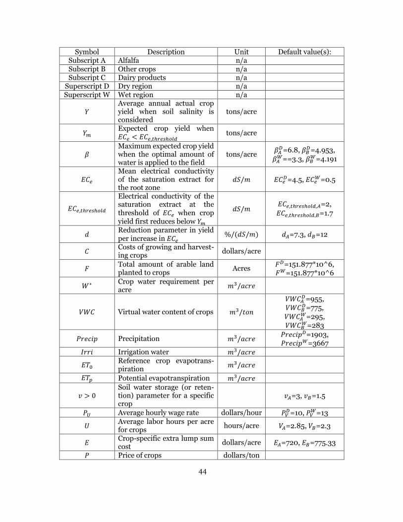
Symbol Description Unit Default value(s): Subscript A Alfalfa n/a Subscript B Other crops n/a Subscript C Dairy products n/a
Superscript D Dry region n/a Superscript W Wet region n/a
𝑌 Average annual actual crop yield when soil salinity is considered
tons/acre
𝑌𝑚 Expected crop yield when 𝐸𝐶𝑒 < 𝐸𝐶𝑒,𝑡ℎ𝑟𝑒𝑠ℎ𝑜𝑙𝑑
tons/acre
𝛽 Maximum expected crop yield when the optimal amount of water is applied to the field
tons/acre 𝛽𝐴
𝐷=6.8, 𝛽𝐵𝐷=4.953,
𝛽𝐴𝑊==3.3, 𝛽𝐵
𝑊=4.191
𝐸𝐶𝑒 Mean electrical conductivity of the saturation extract for the root zone
𝑑𝑆/𝑚 𝐸𝐶𝑒𝐷=4.5, 𝐸𝐶𝑒
𝑊=0.5
𝐸𝐶𝑒,𝑡ℎ𝑟𝑒𝑠ℎ𝑜𝑙𝑑
Electrical conductivity of the saturation extract at the threshold of 𝐸𝐶𝑒 when crop yield first reduces below 𝑌𝑚
𝑑𝑆/𝑚 𝐸𝐶𝑒,𝑡ℎ𝑟𝑒𝑠ℎ𝑜𝑙𝑑,𝐴=2, 𝐸𝐶𝑒,𝑡ℎ𝑟𝑒𝑠ℎ𝑜𝑙𝑑,𝐵=1.7
𝑑 Reduction parameter in yield per increase in 𝐸𝐶𝑒
%/(𝑑𝑆/𝑚) 𝑑𝐴=7.3, 𝑑𝐵=12
𝐶 Costs of growing and harvest-ing crops
dollars/acre
𝐹 Total amount of arable land planted to crops
Acres 𝐹𝐷=151.877*10^6, 𝐹𝑊=151.877*10^6
𝑊∗ Crop water requirement per acre
𝑚3/𝑎𝑐𝑟𝑒
𝑉𝑊𝐶 Virtual water content of crops 𝑚3/𝑡𝑜𝑛
𝑉𝑊𝐶𝐴𝐷=955,
𝑉𝑊𝐶𝐵𝐷=775,
𝑉𝑊𝐶𝐴𝑊=295,
𝑉𝑊𝐶𝐵𝑊=283
𝑃𝑟𝑒𝑐𝑖𝑝 Precipitation 𝑚3/𝑎𝑐𝑟𝑒 𝑃𝑟𝑒𝑐𝑖𝑝𝐷=1903, 𝑃𝑟𝑒𝑐𝑖𝑝𝑊=3667
𝐼𝑟𝑟𝑖 Irrigation water 𝑚3/𝑎𝑐𝑟𝑒
𝐸𝑇0 Reference crop evapotrans-piration
𝑚3/𝑎𝑐𝑟𝑒
𝐸𝑇𝑝 Potential evapotranspiration 𝑚3/𝑎𝑐𝑟𝑒
𝑣 > 0 Soil water storage (or reten-tion) parameter for a specific crop
𝑣𝐴=3, 𝑣𝐵=1.5
𝑃𝑈 Average hourly wage rate dollars/hour 𝑃𝑉𝐷=10, 𝑃𝑉
𝑊=13
𝑈 Average labor hours per acre for crops
hours/acre 𝑉𝐴=2.85, 𝑉𝐵=2.3
𝐸 Crop-specific extra lump sum cost
dollars/acre 𝐸𝐴=720, 𝐸𝐵=775.33
𝑃 Price of crops dollars/ton
45
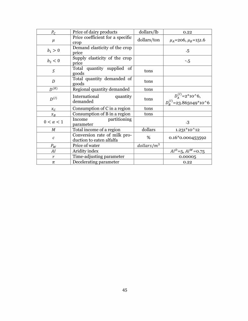
𝑃𝐶 Price of dairy products dollars/lb 0.22
𝜇 Price coefficient for a specific crop
dollars/ton 𝜇𝐴=206, 𝜇𝐵=151.6
𝑏1 > 0 Demand elasticity of the crop price
.5
𝑏2 < 0 Supply elasticity of the crop price
-.5
𝑆 Total quantity supplied of goods
tons
𝐷 Total quantity demanded of goods
tons
𝐷(𝑅) Regional quantity demanded tons
𝐷(𝐼) International quantity demanded
tons 𝐷𝐴
(𝐼)=2*10^6,
𝐷𝐵(𝐼)
=23.865049*10^6
𝑥𝐶 Consumption of C in a region tons
𝑥𝐵 Consumption of B in a region tons
0 < 𝛼 < 1 Income partitioning parameter
.3
𝑀 Total income of a region dollars 1.231*10^12
𝑐 Conversion rate of milk pro-duction to eaten alfalfa
% 0.16*0.000453592
𝑃𝑊 Price of water 𝑑𝑜𝑙𝑙𝑎𝑟𝑠/𝑚3
𝐴𝐼 Aridity index 𝐴𝐼𝐷=5, 𝐴𝐼𝑊=0.75
𝑟 Time-adjusting parameter 0.00005
𝜋 Decelerating parameter 0.22

46
APPENDIX B
MATLAB CODE
47
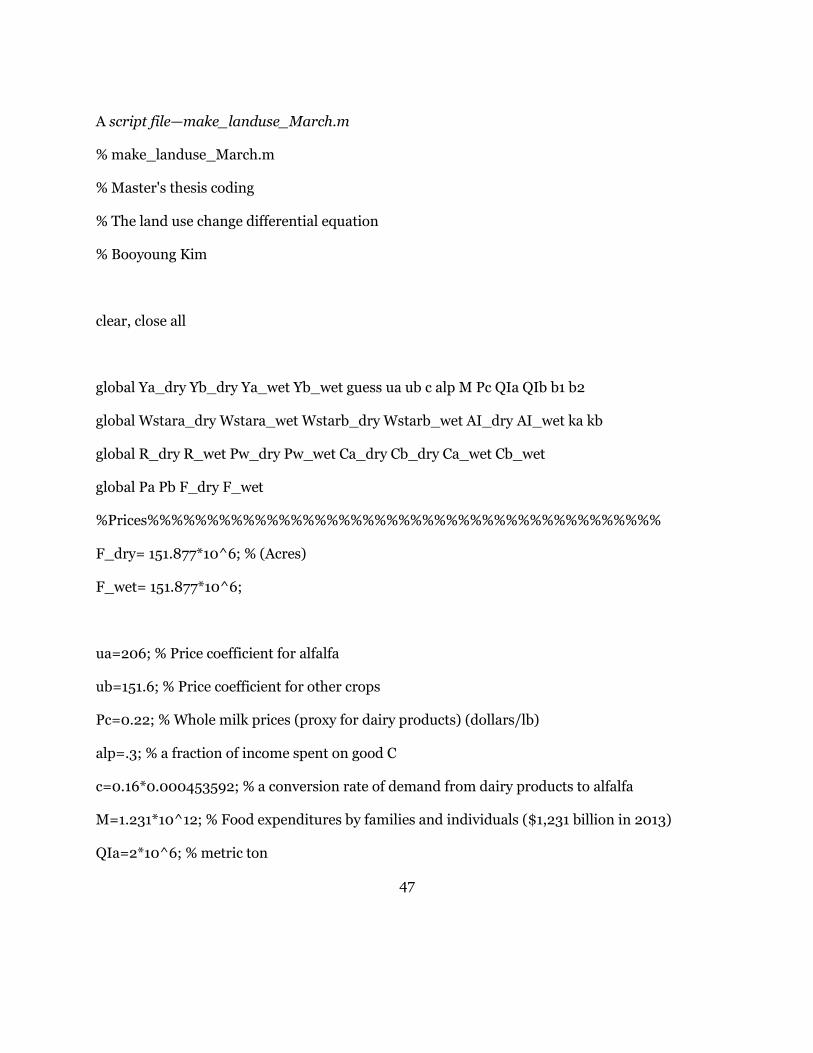
A script file—make_landuse_March.m
% make_landuse_March.m
% Master's thesis coding
% The land use change differential equation
% Booyoung Kim
clear, close all
global Ya_dry Yb_dry Ya_wet Yb_wet guess ua ub c alp M Pc QIa QIb b1 b2
global Wstara_dry Wstara_wet Wstarb_dry Wstarb_wet AI_dry AI_wet ka kb
global R_dry R_wet Pw_dry Pw_wet Ca_dry Cb_dry Ca_wet Cb_wet
global Pa Pb F_dry F_wet
%Prices%%%%%%%%%%%%%%%%%%%%%%%%%%%%%%%%%%%%%%%%%%%
F_dry= 151.877*10^6; % (Acres)
F_wet= 151.877*10^6;
ua=206; % Price coefficient for alfalfa
ub=151.6; % Price coefficient for other crops
Pc=0.22; % Whole milk prices (proxy for dairy products) (dollars/lb)
alp=.3; % a fraction of income spent on good C
c=0.16*0.000453592; % a conversion rate of demand from dairy products to alfalfa
M=1.231*10^12; % Food expenditures by families and individuals ($1,231 billion in 2013)
QIa=2*10^6; % metric ton
48
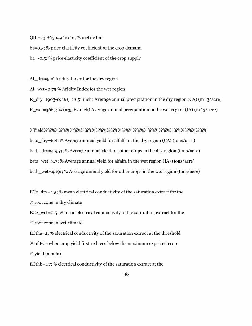
QIb=23.865049*10^6; % metric ton
b1=0.5; % price elasticity coefficient of the crop demand
b2=-0.5; % price elasticity coefficient of the crop supply
AI_dry=5 % Aridity Index for the dry region
AI_wet=0.75 % Aridity Index for the wet region
R_dry=1903-0; % (=18.51 inch) Average annual precipitation in the dry region (CA) (m^3/acre)
R_wet=3667; % (=35.67 inch) Average annual precipitation in the wet region (IA) (m^3/acre)
%Yield%%%%%%%%%%%%%%%%%%%%%%%%%%%%%%%%%%%%%%%%%%%%
beta_dry=6.8; % Average annual yield for alfalfa in the dry region (CA) (tons/acre)
betb_dry=4.953; % Average annual yield for other crops in the dry region (tons/acre)
beta_wet=3.3; % Average annual yield for alfalfa in the wet region (IA) (tons/acre)
betb_wet=4.191; % Average annual yield for other crops in the wet region (tons/acre)
ECe_dry=4.5; % mean electrical conductivity of the saturation extract for the
% root zone in dry climate
ECe_wet=0.5; % mean electrical conductivity of the saturation extract for the
% root zone in wet climate
ECtha=2; % electrical conductivity of the saturation extract at the threshold
% of ECe when crop yield first reduces below the maximum expected crop
% yield (alfalfa)
ECthb=1.7; % electrical conductivity of the saturation extract at the
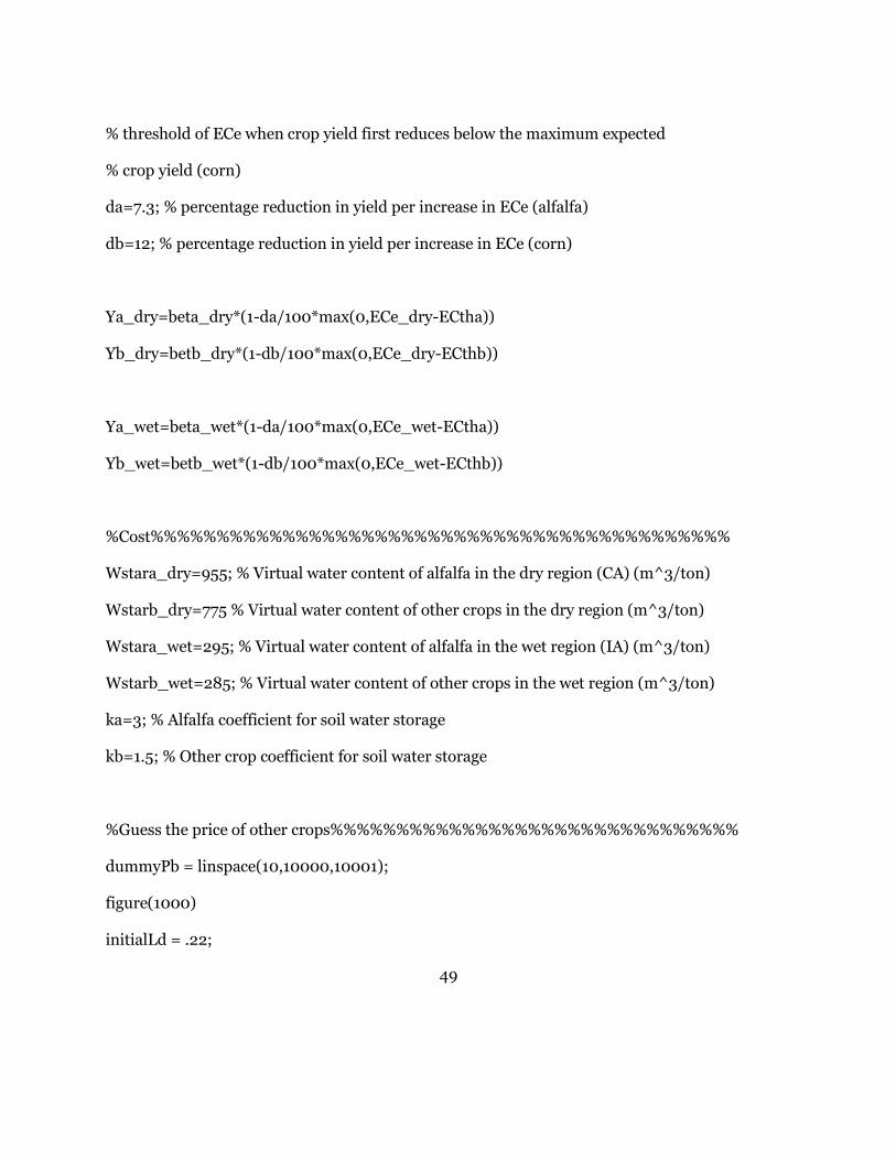
49
% threshold of ECe when crop yield first reduces below the maximum expected
% crop yield (corn)
da=7.3; % percentage reduction in yield per increase in ECe (alfalfa)
db=12; % percentage reduction in yield per increase in ECe (corn)
Ya_dry=beta_dry*(1-da/100*max(0,ECe_dry-ECtha))
Yb_dry=betb_dry*(1-db/100*max(0,ECe_dry-ECthb))
Ya_wet=beta_wet*(1-da/100*max(0,ECe_wet-ECtha))
Yb_wet=betb_wet*(1-db/100*max(0,ECe_wet-ECthb))
%Cost%%%%%%%%%%%%%%%%%%%%%%%%%%%%%%%%%%%%%%%%%%%%
Wstara_dry=955; % Virtual water content of alfalfa in the dry region (CA) (m^3/ton)
Wstarb_dry=775 % Virtual water content of other crops in the dry region (m^3/ton)
Wstara_wet=295; % Virtual water content of alfalfa in the wet region (IA) (m^3/ton)
Wstarb_wet=285; % Virtual water content of other crops in the wet region (m^3/ton)
ka=3; % Alfalfa coefficient for soil water storage
kb=1.5; % Other crop coefficient for soil water storage
%Guess the price of other crops%%%%%%%%%%%%%%%%%%%%%%%%%%%%%%%
dummyPb = linspace(10,10000,10001);
figure(1000)
initialLd = .22;
50
initialLw = .04;
plot(dummyPb,ub*[((1-alp)*M./dummyPb+QIb).^b1*(F_dry*(1-initialLd)*Yb_dry+F_wet*(1-
initialLw)*Yb_wet).^b2]-dummyPb)
hold on
plot([0 10000],[0 0],'--k')
ylim([-1 1])
guess = input('Booyoung, guess Pb!: ')
%%%%%%%%%%%%%%%%%%%%%%%%%%%%%%%%%%%%%%%%%%%%%%%%
[T,V]=ode45(@landuse,[0 100],[initialLd initialLw]);
%Plot%%%%%%%%%%%%%%%%%%%%%%%%%%%%%%%%%%%%%%%%%%%%
figure(1), plot(V(:,1),V(:,2),'k','linewidth',2); hold on
plot(V(1,1),V(1,2),'sqk')
plot(V(end,1),V(end,2),'pk','markersize',12)
% xlim([0 1]), ylim([0 1])
set(gca,'fontsize',16)
% axis equal
xlabel('L_d'), ylabel('L_w')
set(gcf,'position',[100 200 550 450])
figure(2), subplot(2,1,1)
plot(T,V(:,1),'--r','linewidth',2), hold on
plot(T,V(:,2),'b','linewidth',2)
51
set(gca,'fontsize',16)
xlabel('Time'), ylabel('L_d, L_w')
set(gcf,'position',[750 50 600 700])
subplot(2,1,2)
Ld = V(:,1);
Lw = V(:,2);
Pat=ua*[(c*alp*M/Pc+QIa)^b1].*(F_dry*Ld*Ya_dry+F_wet*Lw*Ya_wet).^b2;
for t = 1:length(T)
Pb=fzero(@(Pbx) ub*(((1-alp)*M./Pbx+QIb).^b1)*(F_dry*(1-Ld(t))*Yb_dry+F_wet*(1-
Lw(t))*Yb_wet).^b2-Pbx,guess);
Pbt(t) = Pb;
guess = Pb;
end
plot(T,Pat,'-.','color',[0 0.5 0],'linewidth',2), hold on % green
plot(T,Pbt,'color',[0.5 0 0.5],'linewidth',2), hold on % purple
set(gca,'fontsize',16)
xlabel('Time'), ylabel('Pa, Pb')
A function file—landuse.m
% landuse.m
function dVdt = landuse(t,V)
52
global Ya_dry Yb_dry Ya_wet Yb_wet guess ua ub c alp M Pc QIa QIb b1 b2
global Wstara_dry Wstara_wet Wstarb_dry Wstarb_wet AI_dry AI_wet ka kb
global R_dry R_wet Pw_dry Pw_wet Ca_dry Cb_dry Ca_wet Cb_wet
global Pa Pb F_dry F_wet
Ld = V(1);
Lw = V(2);
%Price%%%%%%%%%%%%%%%%%%%%%%%%%%%%%%%%%%%%%%%%%%%%
Pa=ua*[(c*alp*M/Pc+QIa)^b1]*(F_dry*Ld*Ya_dry+F_wet*Lw*Ya_wet)^b2
Pb=fzero(@(Pbx) ub*(((1-alp)*M./Pbx+QIb).^b1)*(F_dry*(1-Ld)*Yb_dry+F_wet*(1-
Lw)*Yb_wet).^b2-Pbx,guess)
guess = Pb;
Wd_dry=F_dry*Ld*(Ya_dry*Wstara_dry*(1+AI_dry^(-ka))^(1/ka)-R_dry)+F_dry*(1-
Ld)*(Yb_dry*Wstarb_dry*(1+AI_dry^(-kb))^(1/kb)-R_dry)
Wd_wet=F_wet*Lw*(Ya_wet*Wstara_wet*(1+AI_wet^(-ka))^(1/ka)-R_wet)+F_wet*(1-
Lw)*(Yb_wet*Wstarb_wet*(1+AI_wet^(-kb))^(1/kb)-R_wet)
Pw_dry=0.22*(1.001^(Wd_dry/((0.5^AI_dry)*10^10))-1); % the price of water in the dry
region (dollars/m^3)
Pw_wet=0.22*(1.001^(Wd_wet/((0.5^AI_wet)*10^10))-1); % the price of water in the wet
region (dollars/m^3)
Ea=720; % Extra lump sum cost for alfalfa
53
Eb=775.33; % Extra lump sum cost for other crops
Pv_dry=10; % hourly wage rate in the dry region
Pv_wet=13; % hourly wage rate in the wet region
Va=2.85; % labor hours per acre for alfalfa
Vb=2.3; % labor hours per acre for other crops
Ca_dry=Pw_dry*max(0,((Ya_dry*Wstara_dry-0)-R_dry*(1+AI_dry^(-ka))^(-
1/ka)))+Pv_dry*Va+Ea;
Cb_dry=Pw_dry*max(0,(Yb_dry*Wstarb_dry-R_dry*(1+AI_dry^(-kb))^(-
1/kb)))+Pv_dry*Vb+Eb;
Ca_wet=Pw_wet*max(0,(Ya_wet*Wstara_wet-R_wet*(1+AI_wet^(-ka))^(-
1/ka)))+Pv_wet*Va+Ea;
Cb_wet=Pw_wet*max(0,(Yb_wet*Wstarb_wet-R_wet*(1+AI_wet^(-kb))^(-
1/kb)))+Pv_wet*Vb+Eb;
dVdt = zeros(2,1);
dVdt(1) = 0.00005 * Ld*(1-Ld)*[(Pa*Ya_dry-Ca_dry)-(Pb*Yb_dry-Cb_dry)];
dVdt(2) = 0.00005 * Lw*(1-Lw)*((Pa*Ya_wet-Ca_wet)-(Pb*Yb_wet-Cb_wet))
end