Embed Size (px)
Citation preview
Analysis of freeform optical systems based on the
decomposition of the total wave aberration into Zernike
surface contributions
Dissertation
for the acquisition of the academic title
doctor rerum naturalium (Dr. rer. nat.)
submitted to the Council of the Faculty of Physics and Astronomy
of the Friedrich-Schiller-Universität Jena
by
MSc. Mateusz Oleszko
born in Opole, Poland on 10.07.1988

2
Supervisors:
Major Supervisor: Prof. Dr. Herbert Gross
Associate Supervisor: Prof. Dr. Norbert Lindlein
Associate Supervisor: Prof. Dr. Fabian Duerr
Day of the Disputation: 09.04.2019
3
Abstract
The increasing use of freeform optical surfaces raises the demand for optical design tools
developed for generalized systems. In the design process, surface-by-surface aberration
contributions are of special interest. The expansion of the wave aberration function into the
field- and pupil-dependent coefficients is an analytical method used for that purpose. An
alternative numerical approach utilizing data from the trace of multiple ray sets is proposed.
The optical system is divided into segments of the optical path measured along the chief ray.
Each segment covers one surface and the distance to the subsequent surface. Surface
contributions represent the change of the wavefront that occurs due to propagation through
individual segments. Further, the surface contributions are divided with respect to their
phenomenological origin into intrinsic induced and transfer components. Each component is
determined from a separate set of rays. The proposed method does not place any constraints on
the system geometry or the aperture shape. However, in this thesis only plane symmetric
systems with near-circular apertures are studied. This enabled characterization of the obtained
aberration components with Zernike fringe polynomials.
The application of the proposed method in the design process of the freeform systems is
demonstrated. The analysis of Zernike surface contributions provides valuable insights for
selecting the starting system with the best potential for correcting aberrations with freeform
surfaces. Further, it helps in determining the effective location of a freeform element in a
system. Consequently, it is possible to design systems corrected for Zernike aberrations of
order higher than the order of coefficients used for freeform sag contributions, described with
the same Zernike polynomial set.

4
This page is left blank intentionally.
5
Contents
Contents ..................................................................................................................................... 5
Chapter 1 Introduction ............................................................................................................ 8
Chapter 2 Theory .................................................................................................................. 11
2.1 Wave aberrations determined analytically ................................................................ 11
2.1.1 Ray aberrations .................................................................................................... 11
2.1.2 The total wave aberration..................................................................................... 12
2.1.3 The expansion of the wave aberration function ................................................... 13
2.1.4 Wave aberration coefficients in terms of Seidel sums ......................................... 15
2.1.5 Sixth-order wave aberration coefficients ............................................................. 16
2.1.5.1 Intrinsic aberrations .................................................................................... 17
2.1.5.2 Induced aberrations..................................................................................... 18
2.1.6 The wave aberration function in non-rotationally symmetric systems ................ 19
2.1.6.1 Nodal aberration theory .............................................................................. 19
2.1.6.2 Aberration fields of plane symmetric systems ........................................... 21
2.1.7 Pupil coordinates .................................................................................................. 22
2.2 Wave aberrations determined numerically ................................................................ 24
2.2.1 The optical path difference (OPD) formula ......................................................... 24
2.2.2 Alternative definition of surface contributions .................................................... 26
2.2.3 First-order ray tracing .......................................................................................... 27
2.2.3.1 Grid distortion............................................................................................. 28
2.2.3.2 Exit pupil shape .......................................................................................... 28
2.2.4 Pupil distortion – ray aiming................................................................................ 29
2.3 Decomposition of the total wave aberration into Zernike fringe coefficients ........... 30
2.4 Freeform optics ......................................................................................................... 34
2.5 Tolerance sensitivity analysis.................................................................................... 35
Chapter 3 Novel method for decomposition of the total wave aberration............................ 38
3.1 Intermediate references ............................................................................................. 38
3.1.1 Reference spheres ................................................................................................ 38
3.1.2 Intermediate images ............................................................................................. 39
6
3.2 Components of surface contributions determined from the trace of multiple
ray set . ……………………………………………………………………………...40
3.2.1 Boundary shape of reference spheres .................................................................. 45
3.2.2 Zernike surface contributions .............................................................................. 47
3.3 Comparison with analytical results ........................................................................... 47
3.4 Full field analysis ...................................................................................................... 51
3.4.1 Full field displays ................................................................................................. 51
3.4.2 Distortion grid ...................................................................................................... 53
3.5 Implementation.......................................................................................................... 54
3.5.1 User-defined parameters ...................................................................................... 55
3.5.2 Modification of the system .................................................................................. 56
3.5.3 Tracing multiple ray sets ...................................................................................... 58
3.5.4 Special aspects ..................................................................................................... 60
3.5.4.1 Propagation to the exit pupil ....................................................................... 60
3.5.4.2 Vignetting ................................................................................................... 60
3.5.4.3 Position of the entrance pupil ..................................................................... 61
Chapter 4 Application ........................................................................................................... 63
4.1 Relations between low- and higher-order Zernike aberrations ................................. 63
4.2 Selection of the initial system ................................................................................... 64
4.2.1 Geometry of the system ....................................................................................... 65
4.2.2 Zernike surface contributions analysis................................................................. 66
4.2.3 Performance comparison ..................................................................................... 75
4.3 Selection of the surface ............................................................................................. 76
4.4 Misalignment sensitivity analysis ............................................................................. 83
4.5 Analysis of systems with large FOV ......................................................................... 86
Chapter 5 Conclusions .......................................................................................................... 90
Appendix A Performance comparison of methods allowing for communication
between Matlab® and Zemax® ........................................................................... 92
A.1 Possible methods .................................................................................... 92
A.2 Computational speed evaluation ............................................................ 93
References ................................................................................................................................ 95

7
Acknowledgments……………………………………………………………………………99
Zusammenfassung…………………………………………………………………………..101
Curriculum vitae…………………………………………………………………………….103
Publications…………………………………………………………………………………105
Ehrenwörtliche Erklärung…………………………………………………………………..107
8
Chapter 1 Introduction
Before computers became available, lens designers were concentrated on developing tools to
design multi-lens optical systems using simple hand calculation. The introduction of Seidel
sums made the evaluation of primary aberrations of an optical system possible, based only on
construction parameters and a trace of two paraxial rays. That enabled Petzval to design the
first photographic lens corrected for all primary aberrations [1]. The Seidel sums method was
further extended for aberrations of higher orders by Buchdahl [2].
Since the advent of computers the computational power became less of an issue enabling a
trace of multiple real rays through a complete system. Thus, the evaluation of the total
aberration with no limitation to an expansion order has been possible [3]. The lens designers
have employed local optimization methods [4, 5] in the designing process obtaining well-
corrected complex lens systems. Further, in order to explore the complete solution space of a
design problem, different global optimization methods have been tested [6-9]. Nevertheless,
it is still not possible to replace the work of a trained lens designer. Thus in parallel, analytical
approach of expanding wave aberration function into field and pupil-dependent coefficients
has been developed, providing valuable insights into potentials and limitations of a particular
design solution. Currently, surface-by-surface aberration coefficients up to the sixth order are
derived in the literature [10] for axially symmetric systems. The functionality of the approach
has been further extended for the analysis of non-axially symmetric optical systems [11-13].
The analysis of aberration effects is of crucial importance in assessing the limitations and
possibilities of various configurations, guiding the optimization process towards the best „as-
built“ solution [14].
Development of ultraprecision diamond machining technologies enabled the manufacturing of
surfaces with a varying azimuthal profile, the so-called freeforms. This has opened the
possibility to build more compact systems with larger apertures and fields of view [15]. In
order to fully benefit from the application of freeform elements, new mathematical
representations to simulate freeform surfaces in the optical design software were introduced
[16]. In the design stage, typically a set of polynomials is used to describe the complete surface.
9
Global surface representations assure convergence during the optimization process. Thus, new
polynomial sets suitable for different aperture shapes and with different orthogonality
properties [17-19] were developed. After the design stage, it is necessary to assess the
performance of the „as-built“ freeform system. In this case local representations such as radial
basis functions (RBF) appeared to be appropriate to reproduce the manufacturing artifacts [20].
Application of freeform elements in multi-lens imaging system raises an issue of where to place
the freeform surface to be used most effectively. Strategies for placing freeforms to achieve
significant improvement in the performance of multi-lens systems were therefore investigated
by Liu in [21].
However, freeform surfaces appeared to be beneficial especially when applied in tilted mirror
systems. Mirror systems typically consist of only a few surfaces and are non-axially symmetric
in order to avoid central obscuration. Additionally, mirrors generate only monochromatic
aberrations and therefore the choice of glasses is of no concern. Thus, freeform surfaces can be
employed to develop compact tilted mirror systems with excellent imaging performance, large
field of view (FOV) and low F# [15]. However, it is non-trivial to determine which starting
system to choose and where to place the freeform element to obtain the best design. The
knowledge of aberration generated in the system is very helpful in answering these questions.
Thus, design strategies based on aberration theory have been developed in recent years.
One of the approaches presented in [22] is to iteratively identify the limiting aberration and to
apply the correct term in the description of the freeform sag contribution. This approach is
based on modifications to the aberration fields introduced by freeform surfaces derived from
nodal aberration theory (NAT) [23]. The final image performance is then checked in the exit
pupil using full field displays (FFDs) of Zernike aberrations obtained from ray-tracing data.
Another design procedure is to first design an appropriate axially symmetric starting system by
using Gaussian brackets and Seidel aberration coefficients. Next, to apply tilt angles and derive
the aberration coefficients of an unobscured system with NAT. In the last step freeform
elements are introduced to correct the large arising, field-constant aberrations [24].
The aim of this thesis was to develop a new numerical method for determining surface-by-
surface contributions to the total wave aberration that can be used to assist the design of
freeform optical systems. This thesis is divided into three parts. In chapter 2, an overview of
10
the field of wave aberration theory is given. Both analytical and ray-tracing methods to
determine wave aberrations are introduced. In chapter 3, the new numerical approach to
determine wave aberrations utilizing data from the trace of multiple ray sets is described. The
total wave aberration is divided into surface contributions and further decomposed into
intrinsic, induced and transfer components. Each component is determined from a separate set
of rays and characterized by Zernike fringe coefficients. In chapter 4, Zernike aberration
coefficients are used to analyze the aberrations of freeform optical systems. The design strategy
based on the proposed method for tilted three-mirror systems is introduced. The potentials to
determine the most effective initial system and the location of the freeform element are
demonstrated. Further, functionalities of the tool in assisting the design of multi-lens systems
are shown.
11
Chapter 2 Theory
2.1 Wave aberrations determined analytically
This section serves as a brief introduction to the theory of aberrations of optical systems with
circular apertures, based on the expansion of the wave aberration function. It is the established
method for classifying aberrations with respect to the symmetry of the optical system. Further,
the expansion of the wave aberration function allows distinguishing contributions from
individual surfaces to the total wave aberration. The total wave aberration quantifies the
deviation from first-order imagery, which can be modeled with respect to a selected convention
of references. Notation employed in this section corresponds to the one used by Sasian in [25].
2.1.1 Ray aberrations
On top of the diffraction effect resulting from a finite aperture, the resolution of an optical
system is limited due to the deviation from the ideal geometric imagery. The geometric
transformation of a point between object and image planes is typically described with the
Gaussian model. In this model each ray originating from the object plane passes through the
entrance and exit pupil planes, which represent the transformation performed by an optical
system, and intersects the image plane at the scaled coordinates. Thus, each ray can be
described using vectors in two planes, namely the field vector and the pupil vector. In this
approach, the normalized field vector (�⃗⃗� ) is located on the object plane and defines the point
source from which the ray set originates. The normalized pupil vector (𝜌 ) defines the
coordinates of the point in which a particular ray intersects the exit pupil. In the first-order
approximation, rays intersect the image plane and the entrance pupil plane at the equivalent
coordinates. However, the real imagery of an optical system deviates from ideal geometric
12
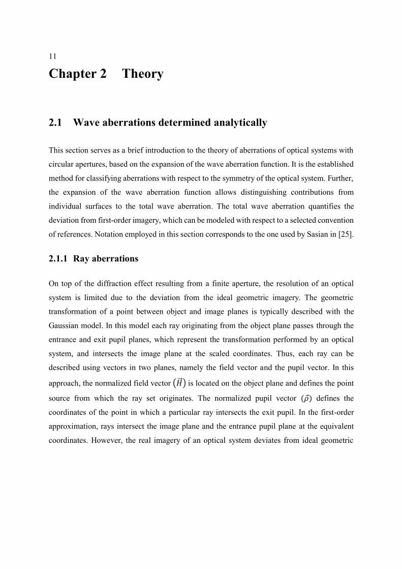
transformation. Consequently, transverse aberrations in the image (𝛥�⃗⃗� ) and the entrance pupil
(𝛥𝜌 ) planes occur; see Figure 2-1.
Figure 2-1. A first-order ray illustrated with the dotted line travels with no transverse error. A real ray, shown
with the solid line, usually travels on a path that deviates from the first-order ray [25].
Here only transverse aberrations of third and fifth order are considered.
2.1.2 The total wave aberration
In the approximation of the first order, each ray originating from a point in the object arrives
at a scaled point in the image, travelling an optical path of the same length measured in the exit
pupil. Nevertheless, if transverse aberrations are added, the optical path for each ray arriving
on the exit pupil differs. Thus, deviation from the ideal imagery can be also expressed in terms
of the error in optical path length (OPL). The OPL is given by integrating the trajectory of a
ray (s) traversing arbitrary points P0 and P1 in a medium with refractive index (n):
𝑂𝑃𝐿 = ∫ 𝑛𝑑𝑠𝑃1
𝑃0. (2-1)
The surface of equal OPL’s is a wavefront. Thus, to determine the wavefront, one needs to
trace an arbitrary set of rays originating from a single point in the object plane.
An ideal wavefront propagates along first-order rays and is a spherical or plane surface that
converges to a point or infinity in the image space. An aberrated wavefront deviates from the
ideal shape. The measure of this deviation in the image space is the total wave aberration.
Further, the wavefront can be well-defined only if the boundary of the beam is unambiguously
determined. This is possible in the mechanical aperture of the optical system. Analogously, the
boundary of the beam is also unblurred in the entrance pupil plane and the exit pupil plane,
13
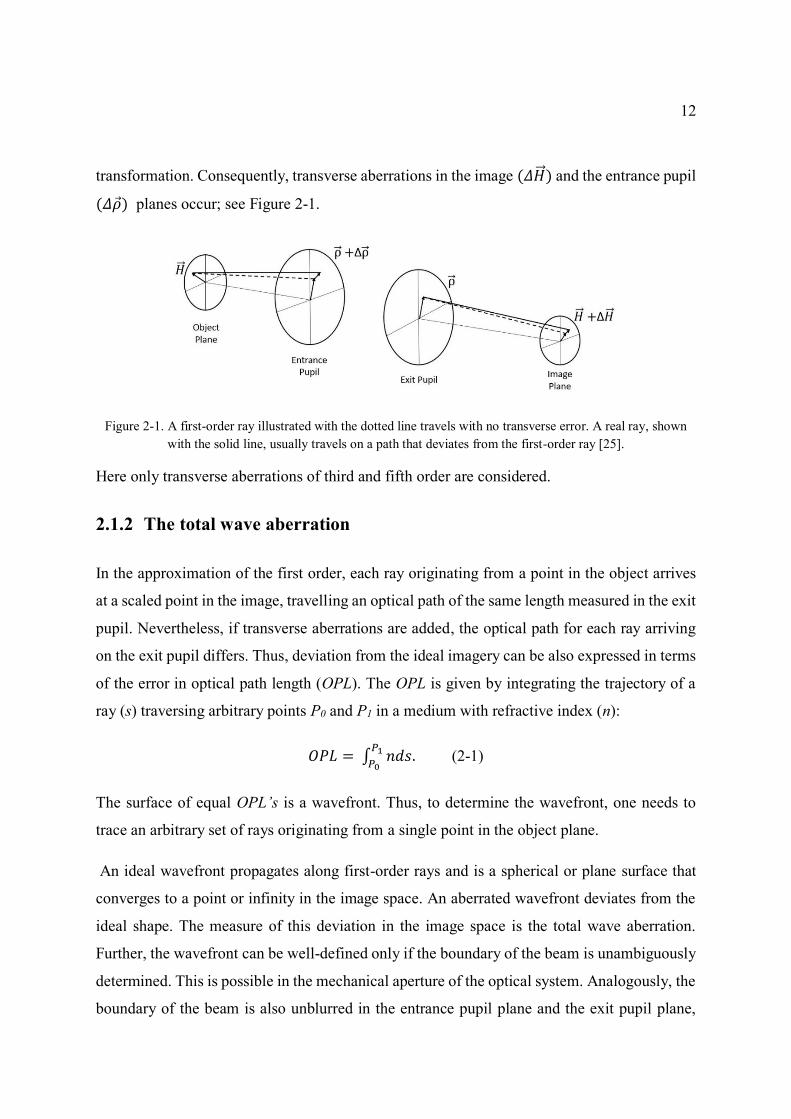
which are the images of the aperture in object and image space, respectively. Thus, the total
wave aberration is defined in the exit pupil as a function of the normalized field and pupil
vectors (𝑊(�⃗⃗� , 𝜌 )). It quantifies the difference in the shape of the real wavefront and the
corresponding ideal wavefront, represented by the reference sphere. This difference is
calculated from the reference sphere to the wavefront along a real ray; see Figure 2-2.
Figure 2-2. The total wave aberration function 𝑊(�⃗⃗� , 𝜌 ) defined as a difference in the shape of the real
wavefront and the corresponding ideal wavefront measured along the real ray in the exit pupil plane.
In analogy, the wave aberration can be defined after each surface in the intermediate exit pupil,
which is an image of the stop in intermediate image space. In this way an optical system is
divided into subsystems each bounded by an associated entrance and exit pupil. Thus,
contributions to the total wave aberration are defined in the exit pupils of individual surfaces.
2.1.3 The expansion of the wave aberration function
Any differentiable function can be approximated by series of coefficients assigned to power
combinations of its variables, known as Taylor series. In principle an unknown function defined
around a certain point in variable space is first approximated to be constant, then a linear
combination, then squared, and so on. For a function 𝑓 of a single variable 𝑥 expanded around
point 𝑥0, one can write:
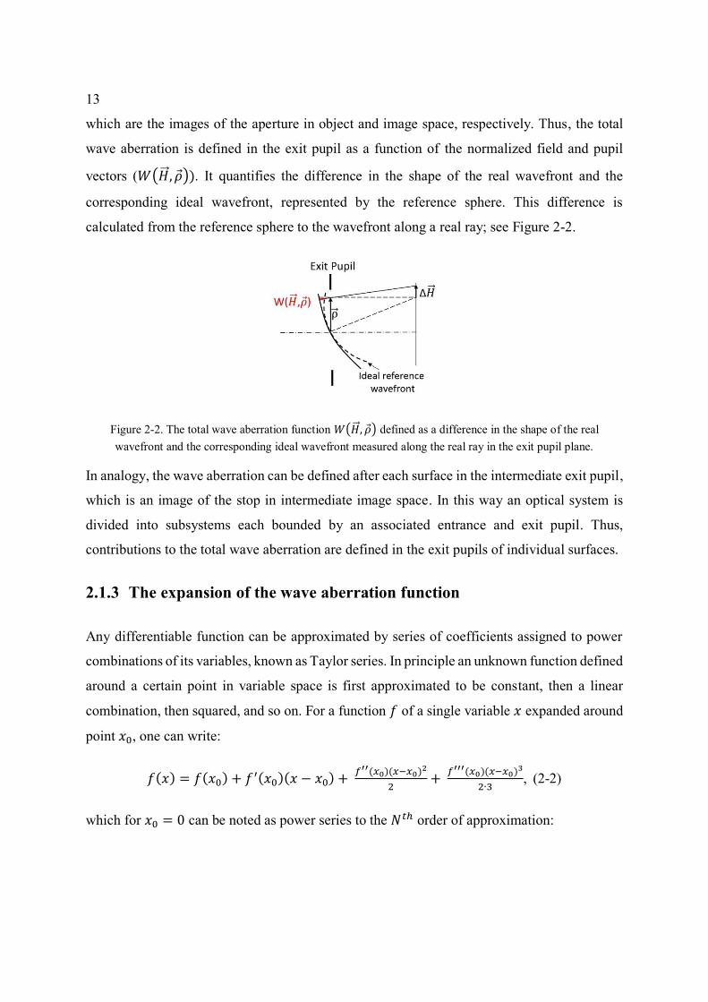
𝑓(𝑥) = 𝑓(𝑥0) + 𝑓′(𝑥0)(𝑥 − 𝑥0) + 𝑓′′(𝑥0)(𝑥−𝑥0)2
2+
𝑓′′′(𝑥0)(𝑥−𝑥0)3
2∙3, (2-2)
which for 𝑥0 = 0 can be noted as power series to the 𝑁𝑡ℎ order of approximation:
14
𝑓(𝑥) = ∑ 𝑎𝑛𝑥𝑛𝑁𝑛 . (2-3)
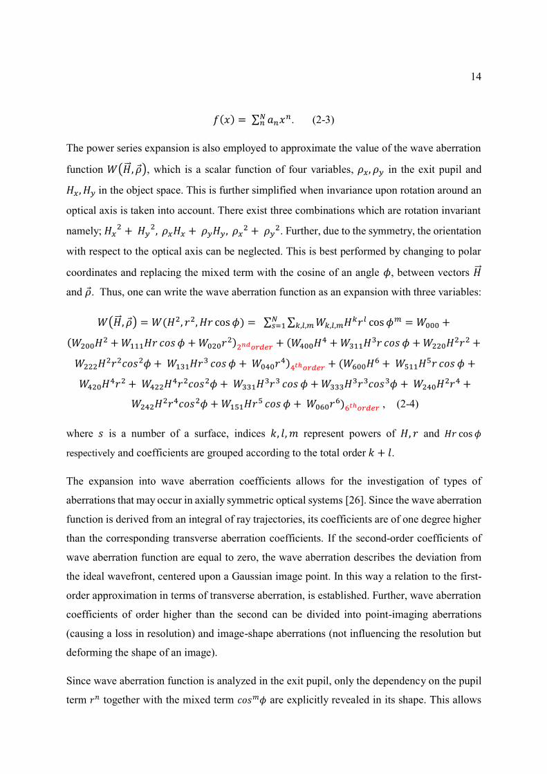
The power series expansion is also employed to approximate the value of the wave aberration
function 𝑊(�⃗⃗� , 𝜌 ), which is a scalar function of four variables, 𝜌𝑥, 𝜌𝑦 in the exit pupil and
𝐻𝑥, 𝐻𝑦 in the object space. This is further simplified when invariance upon rotation around an
optical axis is taken into account. There exist three combinations which are rotation invariant
namely; 𝐻𝑥2 + 𝐻𝑦
2, 𝜌𝑥𝐻𝑥 + 𝜌𝑦𝐻𝑦 , 𝜌𝑥2 + 𝜌𝑦
2. Further, due to the symmetry, the orientation
with respect to the optical axis can be neglected. This is best performed by changing to polar
coordinates and replacing the mixed term with the cosine of an angle 𝜙, between vectors �⃗⃗�
and 𝜌 . Thus, one can write the wave aberration function as an expansion with three variables:
𝑊(�⃗⃗� , 𝜌 ) = 𝑊(𝐻2, 𝑟2, 𝐻𝑟 cos 𝜙) = ∑ ∑ 𝑊𝑘,𝑙,𝑚𝐻𝑘𝑟𝑙 cos 𝜙𝑚𝑘,𝑙,𝑚
𝑁𝑠=1 = 𝑊000 +
(𝑊200𝐻2 + 𝑊111𝐻𝑟 𝑐𝑜𝑠𝜙 + 𝑊020𝑟
2)2𝑛𝑑𝑜𝑟𝑑𝑒𝑟 + (𝑊400𝐻4 + 𝑊311𝐻
3𝑟 𝑐𝑜𝑠 𝜙 + 𝑊220𝐻2𝑟2 +
𝑊222𝐻2𝑟2𝑐𝑜𝑠2𝜙 + 𝑊131𝐻𝑟3 𝑐𝑜𝑠𝜙 + 𝑊040𝑟
4)4𝑡ℎ𝑜𝑟𝑑𝑒𝑟 + (𝑊600𝐻6 + 𝑊511𝐻
5𝑟 𝑐𝑜𝑠 𝜙 +
𝑊420𝐻4𝑟2 + 𝑊422𝐻
4𝑟2𝑐𝑜𝑠2𝜙 + 𝑊331𝐻3𝑟3 𝑐𝑜𝑠 𝜙 + 𝑊333𝐻
3𝑟3𝑐𝑜𝑠3𝜙 + 𝑊240𝐻2𝑟4 +
𝑊242𝐻2𝑟4𝑐𝑜𝑠2𝜙 + 𝑊151𝐻𝑟5 𝑐𝑜𝑠 𝜙 + 𝑊060𝑟
6)6𝑡ℎ𝑜𝑟𝑑𝑒𝑟 , (2-4)
where 𝑠 is a number of a surface, indices 𝑘, 𝑙, 𝑚 represent powers of 𝐻, 𝑟 and 𝐻𝑟 cos𝜙
respectively and coefficients are grouped according to the total order 𝑘 + 𝑙.
The expansion into wave aberration coefficients allows for the investigation of types of
aberrations that may occur in axially symmetric optical systems [26]. Since the wave aberration
function is derived from an integral of ray trajectories, its coefficients are of one degree higher
than the corresponding transverse aberration coefficients. If the second-order coefficients of
wave aberration function are equal to zero, the wave aberration describes the deviation from
the ideal wavefront, centered upon a Gaussian image point. In this way a relation to the first-
order approximation in terms of transverse aberration, is established. Further, wave aberration
coefficients of order higher than the second can be divided into point-imaging aberrations
(causing a loss in resolution) and image-shape aberrations (not influencing the resolution but
deforming the shape of an image).
Since wave aberration function is analyzed in the exit pupil, only the dependency on the pupil
term 𝑟𝑛 together with the mixed term 𝑐𝑜𝑠𝑚𝜙 are explicitly revealed in its shape. This allows
15
for deliberate analysis of point-imaging aberrations, whereas image-shape aberrations are
expressed only through the tilt and decenter with respect to the reference sphere. If azimuthal
order (𝑚) of the pupil dependent coefficient is zero it represents the spherical-like aberration,
which is completely symmetrical about the center of the pupil. In case the index 𝑚 of the
coefficient is equal to one, the aberration has a symmetry about the tangential plane and is
called coma-like. If the aberration has two planes of symmetry (𝑚 is equal to two) it is
classified as astigmatic.
As mentioned, the total wave aberration is a function of two vectors and the sum of
contributions obtained in intermediate exit pupils after each surface. Thus, for sake of
simplicity of analytical derivations introduced in following sections, it is alternatively written
with vector notation:
𝑊(�⃗⃗� , 𝜌 ) = ∑ ∑ 𝑊𝑘,𝑙,𝑚(�⃗⃗� ∙ �⃗⃗� )𝑗∙ (�⃗⃗� ∙ 𝜌 )
𝑚∙ (𝜌 ∙ 𝜌 )𝑛𝑗,𝑚,𝑛
𝑁𝑠=1 , (2-5)
where 𝑠 is a number of a surface, indices 𝑗,𝑚, 𝑛 represent integer numbers related to indices
𝑘, 𝑙,𝑚 of Equation (2-4):
𝑗 = 𝑘−𝑚
2, 𝑚 = 𝑚, 𝑛 =
𝑙−𝑚
2 . (2-6)
This notation is attributed to Roland Shack.
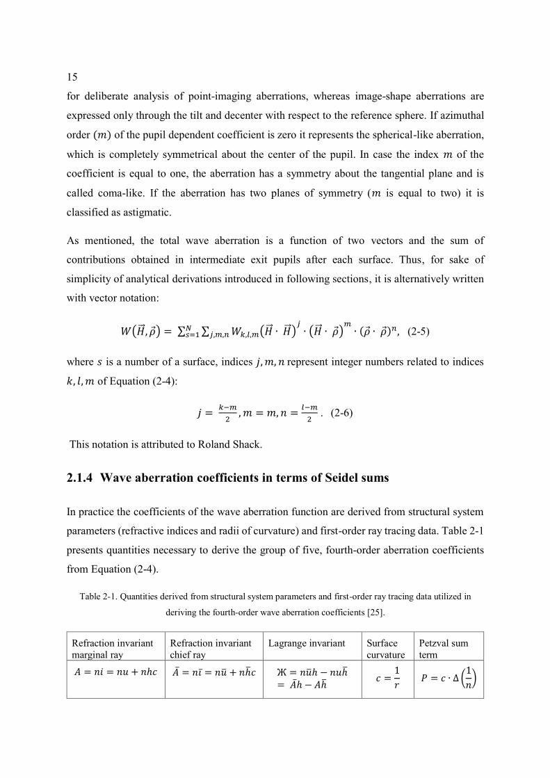
2.1.4 Wave aberration coefficients in terms of Seidel sums
In practice the coefficients of the wave aberration function are derived from structural system
parameters (refractive indices and radii of curvature) and first-order ray tracing data. Table 2-1
presents quantities necessary to derive the group of five, fourth-order aberration coefficients
from Equation (2-4).
Table 2-1. Quantities derived from structural system parameters and first-order ray tracing data utilized in
deriving the fourth-order wave aberration coefficients [25].
Refraction invariant
marginal ray
Refraction invariant
chief ray
Lagrange invariant Surface
curvature
Petzval sum
term
𝐴 = 𝑛𝑖 = 𝑛𝑢 + 𝑛ℎ𝑐 �̅� = 𝑛𝑖̅ = 𝑛�̅� + 𝑛ℎ̅𝑐 Ж = 𝑛�̅�ℎ − 𝑛𝑢ℎ̅= �̅�ℎ − 𝐴ℎ̅
𝑐 =1
𝑟 𝑃 = 𝑐 ∙ ∆ (
1
𝑛)
16
Where 𝑛 is a refractive index, 𝑟 is a radius of curvature, 𝑖 is an incidence angle, 𝑢 is a
convergence angle and ℎ is an incidence height at the surface. The dashed symbols refer to the
first-order chief ray and the ones without dash to the first-order marginal ray.
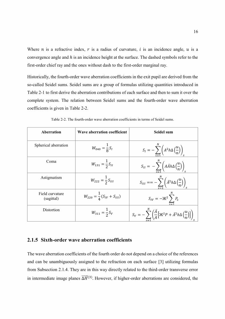
Historically, the fourth-order wave aberration coefficients in the exit pupil are derived from the
so-called Seidel sums. Seidel sums are a group of formulas utilizing quantities introduced in
Table 2-1 to first derive the aberration contributions of each surface and then to sum it over the
complete system. The relation between Seidel sums and the fourth-order wave aberration
coefficients is given in Table 2-2.
Table 2-2. The fourth-order wave aberration coefficients in terms of Seidel sums.
Aberration Wave aberration coefficient Seidel sum
Spherical aberration 𝑊040 =
1
8𝑆𝐼 𝑆𝐼 = −∑(𝐴2ℎ∆ (
𝑢
𝑛))
𝑠
𝑁
𝑠=1
Coma 𝑊131 =
1
2𝑆𝐼𝐼 𝑆𝐼𝐼 = −∑(𝐴�̅�ℎ∆(
𝑢
𝑛))
𝑠
𝑁
𝑠=1
Astigmatism 𝑊222 =
1
2𝑆𝐼𝐼𝐼 𝑆𝐼𝐼𝐼 == −∑ (�̅�2ℎ∆ (
𝑢
𝑛))
𝑠
𝑁
𝑠=1
Field curvature
(sagittal) 𝑊220 =
1
4(𝑆𝐼𝑉 + 𝑆𝐼𝐼𝐼)
𝑆𝐼𝑉 = −Ж2 ∑𝑃𝑠
𝑁
𝑠=1
Distortion 𝑊311 =
1
2𝑆𝑉
𝑆𝑉 = −∑(�̅�
𝐴[Ж2𝑃 + �̅�2ℎ∆ (
𝑢
𝑛)])
𝑠
𝑁
𝑠=1
2.1.5 Sixth-order wave aberration coefficients
The wave aberration coefficients of the fourth order do not depend on a choice of the references
and can be unambiguously assigned to the refraction on each surface [3] utilizing formulas
from Subsection 2.1.4. They are in this way directly related to the third-order transverse error
in intermediate image planes ∆𝐻⃗⃗ ⃗⃗ ⃗(3). However, if higher-order aberrations are considered, the
17
accuracy of the approximation is increased and the transverse error of the pupil vector has to
be taken into account.
In [27] Sasian discusses the strategy for correction of fourth- and sixth-order spherical
aberration introduced by a single element. He concludes, that the higher-order aberrations can
be controlled by a corrector lens system with a known ratio between intersection heights of the
first-order marginal ray and a real, refracted marginal ray, through selecting an appropriate
fourth-order contribution. This ratio is in other words a metric of the transverse pupil aberration
on the corrector lens system introduced by an element under correction.
Consequently, by adding the sixth-order wave aberration coefficients, the third-order
transverse pupil aberration ∆𝜌⃗⃗⃗⃗ ⃗(3) is included. The transverse pupil aberration provides the
mapping error between the entrance pupil and the exit pupil of each surface. This mapping
error arises due to two effects, the refraction on the surface and the incoming aberrated
wavefront.
If the transverse aberration is evaluated at the entrance pupil of each surface, it is possible to
distinguish between these two effects. Thus, the sixth-order aberration coefficients can be
divided into two categories namely, intrinsic and induced. This division was first mentioned
by Hoffman [28] and further developed in [29].
2.1.5.1 Intrinsic aberrations
The intrinsic wave aberration is a deformation of an ideal wavefront after refraction on a
surface evaluated independently on the rest of the system. In this way the sixth-order intrinsic
aberration coefficients are an extension to the fourth-order coefficients taking into account the
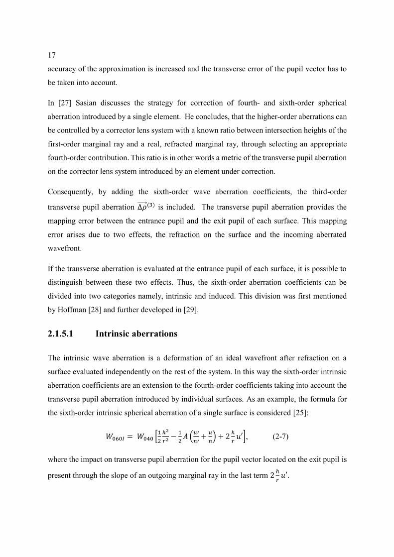
transverse pupil aberration introduced by individual surfaces. As an example, the formula for
the sixth-order intrinsic spherical aberration of a single surface is considered [25]:
𝑊060𝐼 = 𝑊040 [1
2
ℎ2
𝑟2 −1
2𝐴 (
𝑢′
𝑛′+
𝑢
𝑛) + 2
ℎ
𝑟𝑢′], (2-7)
where the impact on transverse pupil aberration for the pupil vector located on the exit pupil is
present through the slope of an outgoing marginal ray in the last term 2ℎ
𝑟𝑢′.
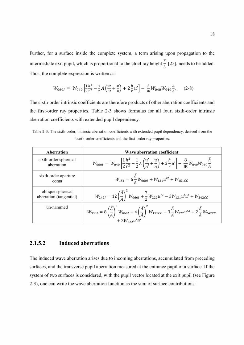
18
Further, for a surface inside the complete system, a term arising upon propagation to the
intermediate exit pupil, which is proportional to the chief ray height ℎ̅
ℎ [25], needs to be added.
Thus, the complete expression is written as:
𝑊060𝐼 = 𝑊040 [1
2
ℎ2
𝑟2 −1
2𝐴(
𝑢′
𝑛′+
𝑢
𝑛) + 2
ℎ
𝑟𝑢′] −
8
Ж𝑊040𝑊040
ℎ̅
ℎ. (2-8)
The sixth-order intrinsic coefficients are therefore products of other aberration coefficients and
the first-order ray properties. Table 2-3 shows formulas for all four, sixth-order intrinsic
aberration coefficients with extended pupil dependency.
Table 2-3. The sixth-order, intrinsic aberration coefficients with extended pupil dependency, derived from the
fourth-order coefficients and the first-order ray properties.
Aberration Wave aberration coefficient
sixth-order spherical
aberration 𝑊060𝐼 = 𝑊040 [1
2
ℎ2
𝑟2 −1
2𝐴 (
𝑢′
𝑛′+
𝑢
𝑛) + 2
ℎ
𝑟𝑢′] −
8
Ж𝑊040𝑊040
ℎ̅
ℎ
sixth-order aperture
coma 𝑊151 = 6�̅�
𝐴𝑊060𝐼 + 𝑊131𝑢
′2 + 𝑊151𝐶𝐶
oblique spherical
aberration (tangential) 𝑊242𝐼 = 12(�̅�
𝐴)
2
𝑊060𝐼 +7
2𝑊222𝑢
′2 − 3𝑊131𝑢′�̅�′ + 𝑊242𝐶𝐶
un-nammed 𝑊333𝐼 = 8(
�̅�
𝐴)
3
𝑊060𝐼 + 4(�̅�
𝐴)
2
𝑊151𝐶𝐶 + 3�̅�
𝐴𝑊222𝑢
′2 + 2�̅�
𝐴𝑊242𝐶𝐶
+ 2𝑊222𝑢′�̅�′
2.1.5.2 Induced aberrations
The induced wave aberration arises due to incoming aberrations, accumulated from preceding
surfaces, and the transverse pupil aberration measured at the entrance pupil of a surface. If the
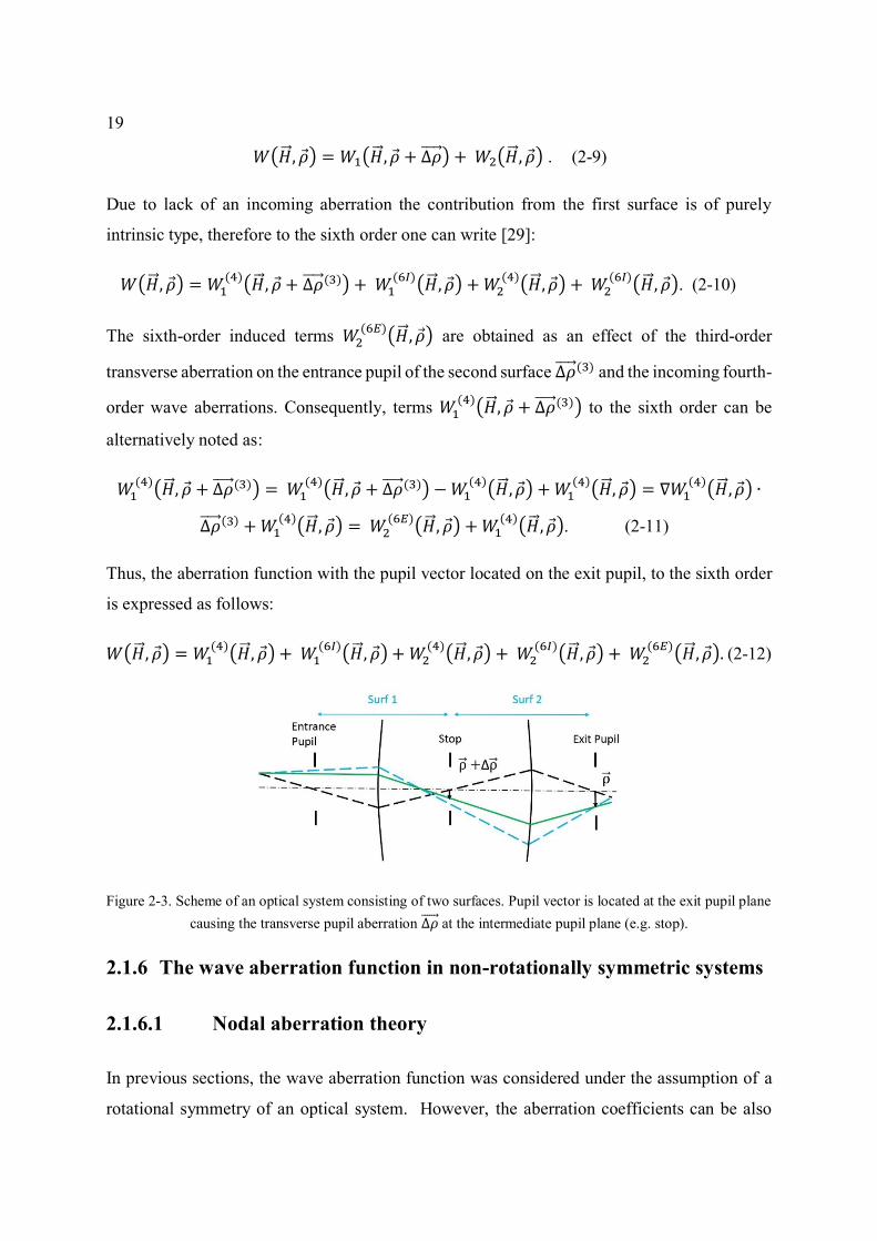
system of two surfaces is considered, with the pupil vector located at the exit pupil (see Figure
2-3), one can write the wave aberration function as the sum of surface contributions:
19
𝑊(�⃗⃗� , 𝜌 ) = 𝑊1(�⃗⃗� , 𝜌 + ∆𝜌⃗⃗⃗⃗ ⃗) + 𝑊2(�⃗⃗� , 𝜌 ) . (2-9)
Due to lack of an incoming aberration the contribution from the first surface is of purely
intrinsic type, therefore to the sixth order one can write [29]:
𝑊(�⃗⃗� , 𝜌 ) = 𝑊1(4)(�⃗⃗� , 𝜌 + ∆𝜌⃗⃗⃗⃗ ⃗(3)) + 𝑊1
(6𝐼)(�⃗⃗� , 𝜌 ) + 𝑊2(4)(�⃗⃗� , 𝜌 ) + 𝑊2
(6𝐼)(�⃗⃗� , 𝜌 ). (2-10)
The sixth-order induced terms 𝑊2(6𝐸)(�⃗⃗� , 𝜌 ) are obtained as an effect of the third-order
transverse aberration on the entrance pupil of the second surface ∆𝜌⃗⃗⃗⃗ ⃗(3) and the incoming fourth-
order wave aberrations. Consequently, terms 𝑊1(4)(�⃗⃗� , 𝜌 + ∆𝜌⃗⃗⃗⃗ ⃗(3)) to the sixth order can be
alternatively noted as:
𝑊1(4)(�⃗⃗� , 𝜌 + ∆𝜌⃗⃗⃗⃗ ⃗(3)) = 𝑊1
(4)(�⃗⃗� , 𝜌 + ∆𝜌⃗⃗⃗⃗ ⃗(3)) − 𝑊1(4)
(�⃗⃗� , 𝜌 ) + 𝑊1(4)
(�⃗⃗� , 𝜌 ) = ∇𝑊1(4)
(�⃗⃗� , 𝜌 ) ∙
∆𝜌⃗⃗⃗⃗ ⃗(3) + 𝑊1(4)
(�⃗⃗� , 𝜌 ) = 𝑊2(6𝐸)(�⃗⃗� , 𝜌 ) + 𝑊1
(4)(�⃗⃗� , 𝜌 ). (2-11)
Thus, the aberration function with the pupil vector located on the exit pupil, to the sixth order
is expressed as follows:
𝑊(�⃗⃗� , 𝜌 ) = 𝑊1(4)(�⃗⃗� , 𝜌 ) + 𝑊1
(6𝐼)(�⃗⃗� , 𝜌 ) + 𝑊2(4)(�⃗⃗� , 𝜌 ) + 𝑊2
(6𝐼)(�⃗⃗� , 𝜌 ) + 𝑊2(6𝐸)(�⃗⃗� , 𝜌 ). (2-12)
Figure 2-3. Scheme of an optical system consisting of two surfaces. Pupil vector is located at the exit pupil plane
causing the transverse pupil aberration ∆𝜌⃗⃗⃗⃗ ⃗ at the intermediate pupil plane (e.g. stop).
2.1.6 The wave aberration function in non-rotationally symmetric systems
2.1.6.1 Nodal aberration theory
In previous sections, the wave aberration function was considered under the assumption of a
rotational symmetry of an optical system. However, the aberration coefficients can be also
20
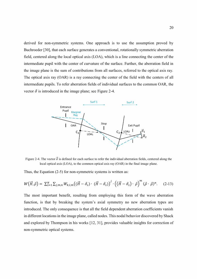
derived for non-symmetric systems. One approach is to use the assumption proved by
Buchroeder [30], that each surface generates a conventional, rotationally symmetric aberration
field, centered along the local optical axis (LOA), which is a line connecting the center of the
intermediate pupil with the center of curvature of the surface. Further, the aberration field in
the image plane is the sum of contributions from all surfaces, referred to the optical axis ray.
The optical axis ray (OAR) is a ray connecting the center of the field with the centers of all
intermediate pupils. To refer aberration fields of individual surfaces to the common OAR, the
vector 𝜎 is introduced in the image plane; see Figure 2-4.
Figure 2-4. The vector �⃗� is defined for each surface to refer the individual aberration fields, centered along the
local optical axis (LOA), to the common optical axis ray (OAR) in the final image plane.
Thus, the Equation (2-5) for non-symmetric systems is written as:
𝑊(�⃗⃗� , 𝜌 ) = ∑ ∑ 𝑊𝑘,𝑙,𝑚((�⃗⃗� − 𝜎 𝑠) ∙ (�⃗⃗� − 𝜎 𝑠))𝑗∙ ((�⃗⃗� − 𝜎 𝑠) ∙ 𝜌 )
𝑚(𝜌 ∙ 𝜌 )𝑛.𝑗,𝑚,𝑛
𝑁𝑠=1 (2-13)
The most important benefit, resulting from employing this form of the wave aberration
function, is that by breaking the system’s axial symmetry no new aberration types are
introduced. The only consequence is that all the field dependent aberration coefficients vanish
in different locations in the image plane, called nodes. This nodal behavior discovered by Shack
and explored by Thompson in his works [12, 31], provides valuable insights for correction of
non-symmetric optical systems.
21
2.1.6.2 Aberration fields of plane symmetric systems
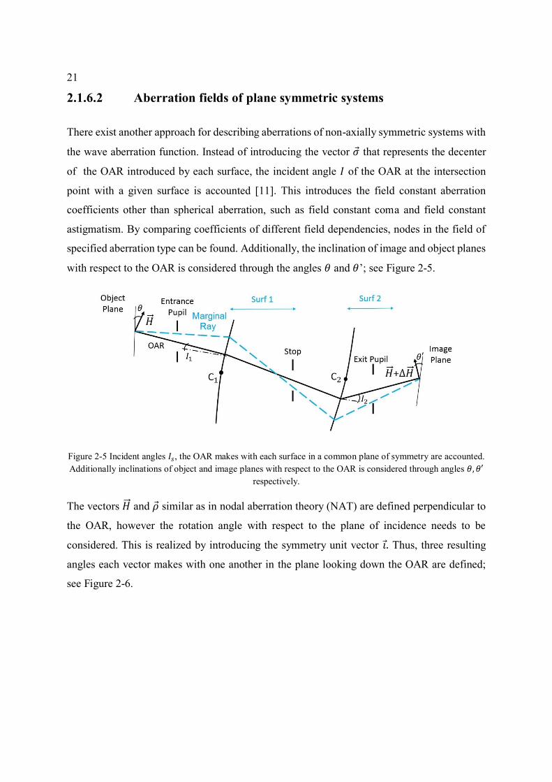
There exist another approach for describing aberrations of non-axially symmetric systems with
the wave aberration function. Instead of introducing the vector 𝜎 that represents the decenter
of the OAR introduced by each surface, the incident angle 𝐼 of the OAR at the intersection
point with a given surface is accounted [11]. This introduces the field constant aberration
coefficients other than spherical aberration, such as field constant coma and field constant
astigmatism. By comparing coefficients of different field dependencies, nodes in the field of
specified aberration type can be found. Additionally, the inclination of image and object planes
with respect to the OAR is considered through the angles 𝜃 and 𝜃’; see Figure 2-5.
Figure 2-5 Incident angles 𝐼𝑠, the OAR makes with each surface in a common plane of symmetry are accounted.
Additionally inclinations of object and image planes with respect to the OAR is considered through angles 𝜃, 𝜃′
respectively.
The vectors �⃗⃗� and 𝜌 similar as in nodal aberration theory (NAT) are defined perpendicular to
the OAR, however the rotation angle with respect to the plane of incidence needs to be
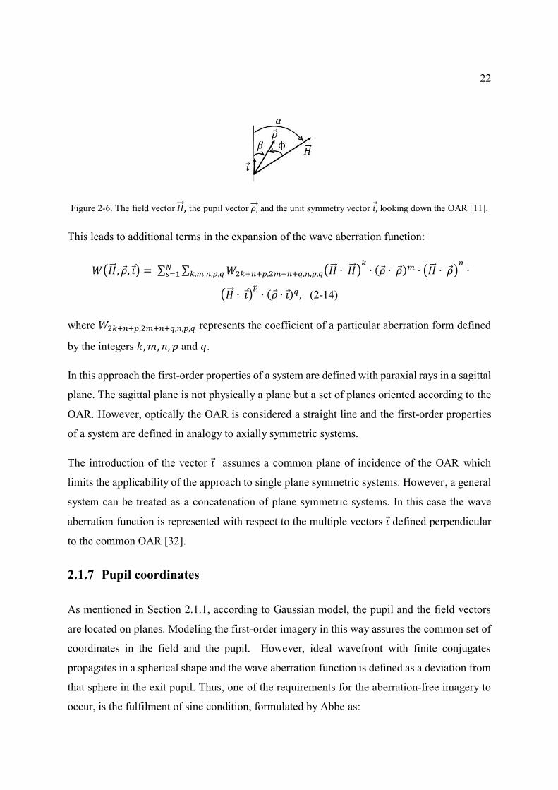
considered. This is realized by introducing the symmetry unit vector 𝑖 . Thus, three resulting
angles each vector makes with one another in the plane looking down the OAR are defined;
see Figure 2-6.
22
Figure 2-6. The field vector �⃗⃗� , the pupil vector 𝜌,⃗⃗ and the unit symmetry vector 𝑖, looking down the OAR [11].
This leads to additional terms in the expansion of the wave aberration function:
𝑊(�⃗⃗� , 𝜌 , 𝑖 ) = ∑ ∑ 𝑊2𝑘+𝑛+𝑝,2𝑚+𝑛+𝑞,𝑛,𝑝,𝑞(�⃗⃗� ∙ �⃗⃗� )𝑘∙ (𝜌 ∙ 𝜌 )𝑚 ∙ (�⃗⃗� ∙ 𝜌 )
𝑛
𝑘,𝑚,𝑛,𝑝,𝑞𝑁𝑠=1 ∙
(�⃗⃗� ∙ 𝑖 )𝑝∙ (𝜌 ∙ 𝑖 )𝑞, (2-14)
where 𝑊2𝑘+𝑛+𝑝,2𝑚+𝑛+𝑞,𝑛,𝑝,𝑞 represents the coefficient of a particular aberration form defined
by the integers 𝑘,𝑚, 𝑛, 𝑝 and 𝑞.
In this approach the first-order properties of a system are defined with paraxial rays in a sagittal
plane. The sagittal plane is not physically a plane but a set of planes oriented according to the
OAR. However, optically the OAR is considered a straight line and the first-order properties
of a system are defined in analogy to axially symmetric systems.
The introduction of the vector 𝑖 assumes a common plane of incidence of the OAR which
limits the applicability of the approach to single plane symmetric systems. However, a general
system can be treated as a concatenation of plane symmetric systems. In this case the wave
aberration function is represented with respect to the multiple vectors 𝑖 defined perpendicular
to the common OAR [32].
2.1.7 Pupil coordinates
As mentioned in Section 2.1.1, according to Gaussian model, the pupil and the field vectors
are located on planes. Modeling the first-order imagery in this way assures the common set of
coordinates in the field and the pupil. However, ideal wavefront with finite conjugates
propagates in a spherical shape and the wave aberration function is defined as a deviation from
that sphere in the exit pupil. Thus, one of the requirements for the aberration-free imagery to
occur, is the fulfilment of sine condition, formulated by Abbe as:
23
sin𝑈
𝑢=
sin𝑈′
𝑢′, (2-15)
where 𝑈 and 𝑈′ are slope angles of real rays before and after refraction, and 𝑢 and 𝑢′ are slopes
of paraxial rays [33]. Paraxial rays are rays close to the optical axis, so the law of refraction
can be approximated with the first-order term in Taylor expansion, which yields that sine
function is expressed as:
sin 𝑢 = 𝑢. (2-16)
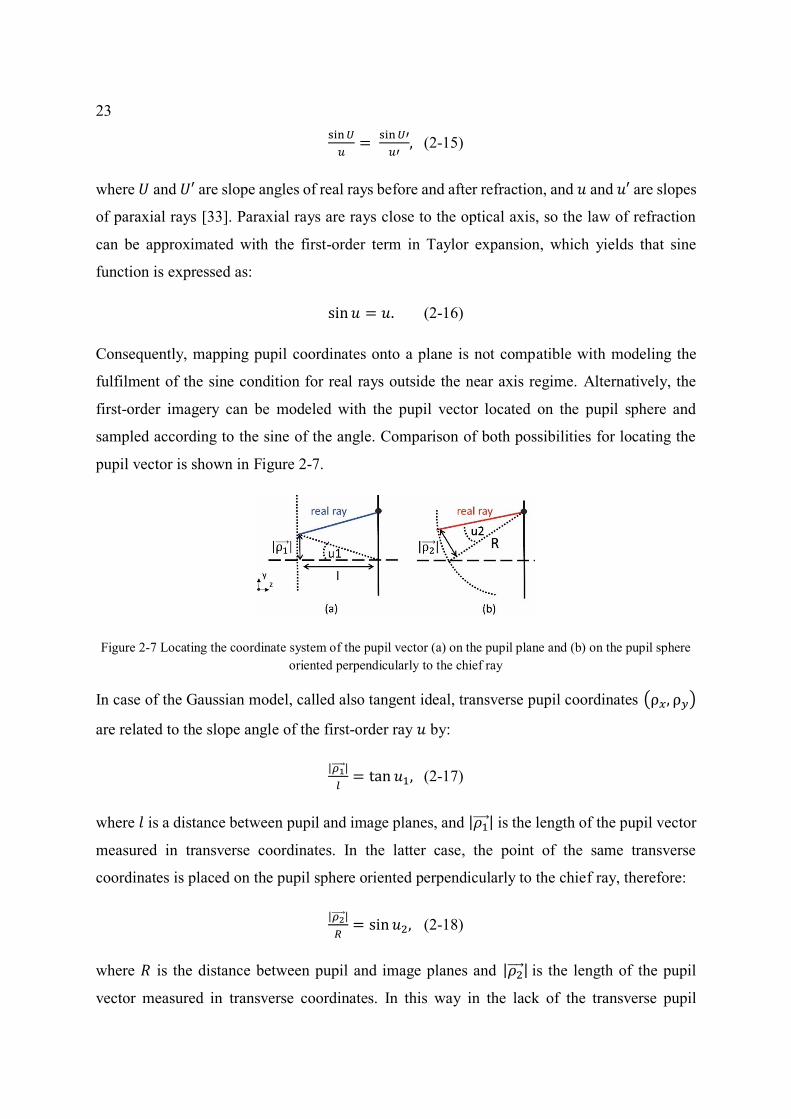
Consequently, mapping pupil coordinates onto a plane is not compatible with modeling the
fulfilment of the sine condition for real rays outside the near axis regime. Alternatively, the
first-order imagery can be modeled with the pupil vector located on the pupil sphere and
sampled according to the sine of the angle. Comparison of both possibilities for locating the
pupil vector is shown in Figure 2-7.
Figure 2-7 Locating the coordinate system of the pupil vector (a) on the pupil plane and (b) on the pupil sphere
oriented perpendicularly to the chief ray
In case of the Gaussian model, called also tangent ideal, transverse pupil coordinates (ρ𝑥, ρ𝑦)
are related to the slope angle of the first-order ray 𝑢 by:
|𝜌1⃗⃗ ⃗⃗ |
𝑙= tan 𝑢1, (2-17)
where 𝑙 is a distance between pupil and image planes, and |𝜌1⃗⃗⃗⃗ | is the length of the pupil vector
measured in transverse coordinates. In the latter case, the point of the same transverse
coordinates is placed on the pupil sphere oriented perpendicularly to the chief ray, therefore:
|𝜌2⃗⃗ ⃗⃗ |
𝑅= sin 𝑢2, (2-18)
where 𝑅 is the distance between pupil and image planes and |𝜌2⃗⃗⃗⃗ | is the length of the pupil
vector measured in transverse coordinates. In this way in the lack of the transverse pupil
24
aberrations 𝛥𝜌 the ideal imagery can be fulfilled also for real rays with large slope angles, if
this occurs optical system is called isoplanatic. Choosing pupil spheres as the reference for the
pupil transverse coordinates is also suitable for calculations of diffraction image theory [34].
However, mapping of an object plane onto an image plane by the way of pupil spheres
introduces ambiguity that each field point is assigned a reference sphere with a different radius
of curvature. This can be avoided by employing an ideal imagery model in which the field
vector is also located on a sphere in object and image spaces, termed the sine ideal [35]. Lens
designers are nevertheless more interested in properties of systems imaging onto plane sensor
surfaces. Thus, similarly as in [28] the “hybrid” model with object and image planes and pupil
spheres is selected further in this thesis.
2.2 Wave aberrations determined numerically
The wave aberration function can be also determined directly from the ray tracing data by
evaluating OPL values for each ray in the exit pupil. In contrary to the analytical approach
presented in the previous section, this approach does not employ any approximations. Thus, no
limitations are imposed on the level of accuracy of the obtained wave aberration, except for
discretization. Moreover, suitable references can be selected without complicated derivations
resulting from any discrepancy from a first-order imagery model.
2.2.1 The optical path difference (OPD) formula
A wavefront is defined as a surface of equal OPL’s measured along rays originating from a
single field point. In order to determine the direction of propagation, the reference ray is
needed. The wavefront error is then defined as a deviation from the shape of an ideal spherical
wavefront, centered along the reference ray. To evaluate the total wave aberration, first the
reference sphere is constructed in the exit pupil and the OPL for each ray is determined. Further
the optical path difference (OPD) with the OPL of the reference ray is calculated:
25
𝑂𝑃𝐷 = 𝑂𝑃𝐿𝑟𝑒𝑓 − 𝑂𝑃𝐿𝑟𝑎𝑦 (2-19)
The OPD map is created based on the intersection coordinates of each ray (𝜌 ) at the selected
pupil.
To establish a relation with the ideal imagery model, the first-order chief ray is selected as the
reference ray. It intersects the image plane and the object plane at the same normalized
coordinates, determined with the field vector �⃗⃗� . Thus, the field dependency is included in each
calculated OPD, and after scaling the OPD map with the wavelength, one can write:
𝑊𝑡𝑜𝑡(�⃗⃗� , 𝜌 ) = 𝑂𝑃𝐷(�⃗⃗� )
𝜆. (2-20)
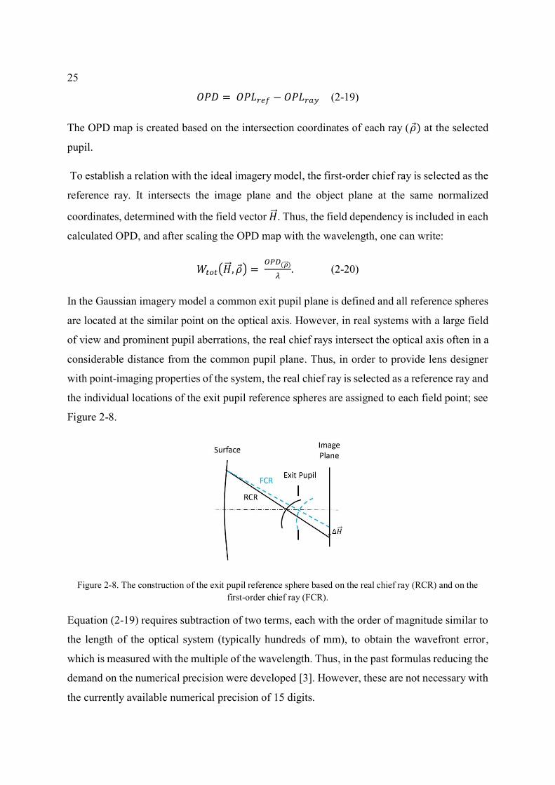
In the Gaussian imagery model a common exit pupil plane is defined and all reference spheres
are located at the similar point on the optical axis. However, in real systems with a large field
of view and prominent pupil aberrations, the real chief rays intersect the optical axis often in a
considerable distance from the common pupil plane. Thus, in order to provide lens designer
with point-imaging properties of the system, the real chief ray is selected as a reference ray and
the individual locations of the exit pupil reference spheres are assigned to each field point; see
Figure 2-8.
Figure 2-8. The construction of the exit pupil reference sphere based on the real chief ray (RCR) and on the
first-order chief ray (FCR).
Equation (2-19) requires subtraction of two terms, each with the order of magnitude similar to
the length of the optical system (typically hundreds of mm), to obtain the wavefront error,
which is measured with the multiple of the wavelength. Thus, in the past formulas reducing the
demand on the numerical precision were developed [3]. However, these are not necessary with
the currently available numerical precision of 15 digits.
26
2.2.2 Alternative definition of surface contributions
In the Gaussian model each surface has an associated entrance and exit pupil plane centered
upon the optical axis (OA). In this way the exit pupil of one surface is at the same time the
entrance pupil of the subsequent surface. Thus, surface contributions are defined as the change
of the wavefront resulting from refraction on the surface and propagation between the
corresponding pupil planes. This overlap is however only possible to define for axially
symmetric systems. As mentioned in Section 2.2.1, the real chief ray (RCR) typically intersects
the optical axis in a considerable distance from the first-order chief ray intersection point, so
the position of the common pupil plane cannot be unambiguously defined for all field points.
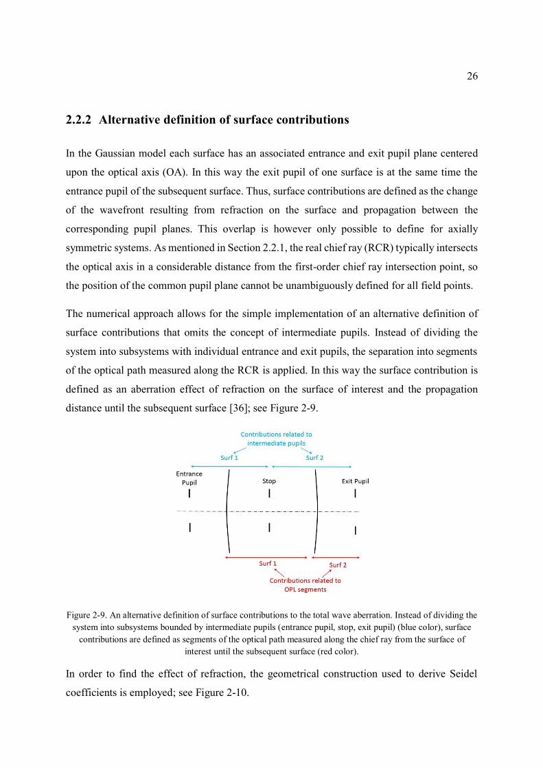
The numerical approach allows for the simple implementation of an alternative definition of
surface contributions that omits the concept of intermediate pupils. Instead of dividing the
system into subsystems with individual entrance and exit pupils, the separation into segments
of the optical path measured along the RCR is applied. In this way the surface contribution is
defined as an aberration effect of refraction on the surface of interest and the propagation
distance until the subsequent surface [36]; see Figure 2-9.
Figure 2-9. An alternative definition of surface contributions to the total wave aberration. Instead of dividing the
system into subsystems bounded by intermediate pupils (entrance pupil, stop, exit pupil) (blue color), surface
contributions are defined as segments of the optical path measured along the chief ray from the surface of
interest until the subsequent surface (red color).
In order to find the effect of refraction, the geometrical construction used to derive Seidel
coefficients is employed; see Figure 2-10.
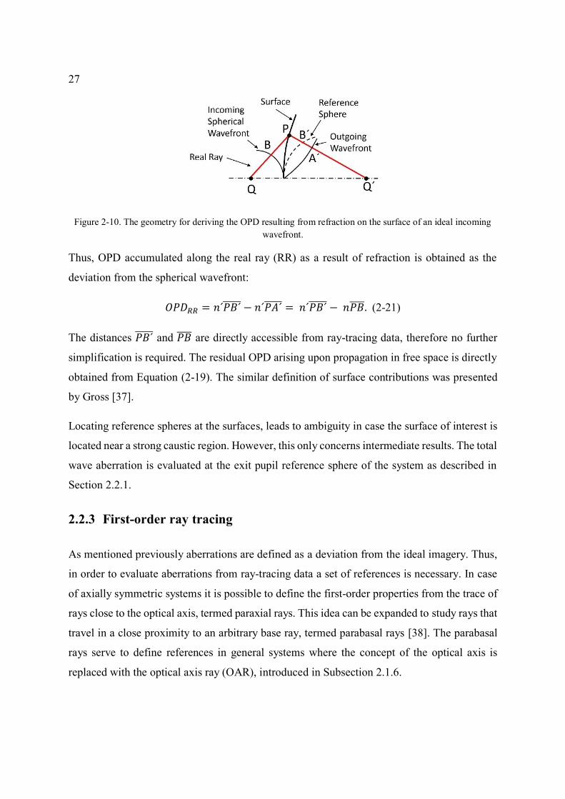
27
Figure 2-10. The geometry for deriving the OPD resulting from refraction on the surface of an ideal incoming
wavefront.
Thus, OPD accumulated along the real ray (RR) as a result of refraction is obtained as the
deviation from the spherical wavefront:
𝑂𝑃𝐷𝑅𝑅 = 𝑛´𝑃𝐵´̅̅ ̅̅ ̅ − 𝑛´𝑃𝐴´̅̅ ̅̅ ̅ = 𝑛´𝑃𝐵´̅̅ ̅̅ ̅ − 𝑛𝑃𝐵̅̅ ̅̅ . (2-21)
The distances 𝑃𝐵´̅̅ ̅̅ ̅ and 𝑃𝐵̅̅ ̅̅ are directly accessible from ray-tracing data, therefore no further
simplification is required. The residual OPD arising upon propagation in free space is directly
obtained from Equation (2-19). The similar definition of surface contributions was presented
by Gross [37].
Locating reference spheres at the surfaces, leads to ambiguity in case the surface of interest is
located near a strong caustic region. However, this only concerns intermediate results. The total
wave aberration is evaluated at the exit pupil reference sphere of the system as described in
Section 2.2.1.
2.2.3 First-order ray tracing
As mentioned previously aberrations are defined as a deviation from the ideal imagery. Thus,
in order to evaluate aberrations from ray-tracing data a set of references is necessary. In case
of axially symmetric systems it is possible to define the first-order properties from the trace of
rays close to the optical axis, termed paraxial rays. This idea can be expanded to study rays that
travel in a close proximity to an arbitrary base ray, termed parabasal rays [38]. The parabasal
rays serve to define references in general systems where the concept of the optical axis is
replaced with the optical axis ray (OAR), introduced in Subsection 2.1.6.
28
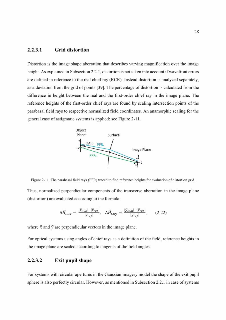
2.2.3.1 Grid distortion
Distortion is the image shape aberration that describes varying magnification over the image
height. As explained in Subsection 2.2.1, distortion is not taken into account if wavefront errors
are defined in reference to the real chief ray (RCR). Instead distortion is analyzed separately,
as a deviation from the grid of points [39]. The percentage of distortion is calculated from the
difference in height between the real and the first-order chief ray in the image plane. The
reference heights of the first-order chief rays are found by scaling intersection points of the
parabasal field rays to respective normalized field coordinates. An anamorphic scaling for the
general case of astigmatic systems is applied; see Figure 2-11.
Figure 2-11. The parabasal field rays (PFR) traced to find reference heights for evaluation of distortion grid.
Thus, normalized perpendicular components of the transverse aberration in the image plane
(distortion) are evaluated according to the formula:
∆�⃗⃗� 𝐶𝑅𝑥 = |𝑥 𝑅𝐶𝑅|−|𝑥 𝑟𝑒𝑓|
|𝑥 𝑟𝑒𝑓|, ∆�⃗⃗� 𝐶𝑅𝑦 =
|�⃗� 𝑅𝐶𝑅|−|�⃗� 𝑟𝑒𝑓|
|�⃗� 𝑟𝑒𝑓| , (2-22)
where 𝑥 and 𝑦 are perpendicular vectors in the image plane.
For optical systems using angles of chief rays as a definition of the field, reference heights in
the image plane are scaled according to tangents of the field angles.
2.2.3.2 Exit pupil shape
For systems with circular apertures in the Gaussian imagery model the shape of the exit pupil
sphere is also perfectly circular. However, as mentioned in Subsection 2.2.1 in case of systems
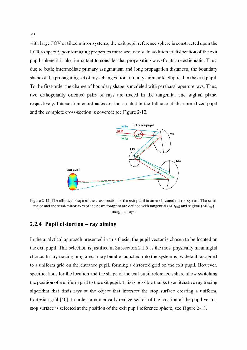
29
with large FOV or tilted mirror systems, the exit pupil reference sphere is constructed upon the
RCR to specify point-imaging properties more accurately. In addition to dislocation of the exit
pupil sphere it is also important to consider that propagating wavefronts are astigmatic. Thus,
due to both; intermediate primary astigmatism and long propagation distances, the boundary
shape of the propagating set of rays changes from initially circular to elliptical in the exit pupil.
To the first-order the change of boundary shape is modeled with parabasal aperture rays. Thus,
two orthogonally oriented pairs of rays are traced in the tangential and sagittal plane,
respectively. Intersection coordinates are then scaled to the full size of the normalized pupil
and the complete cross-section is covered; see Figure 2-12.
Figure 2-12. The elliptical shape of the cross-section of the exit pupil in an unobscured mirror system. The semi-
major and the semi-minor axes of the beam footprint are defined with tangential (MRtan) and sagittal (MRsag)
marginal rays.
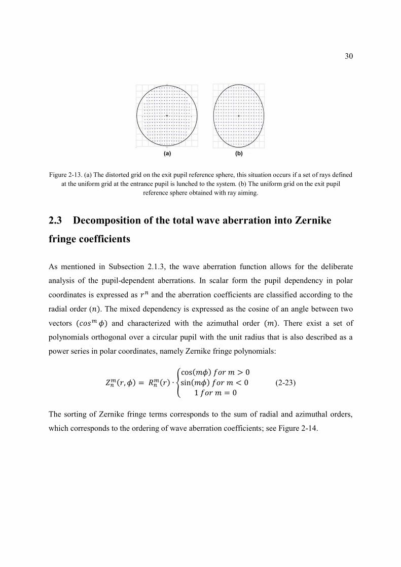
2.2.4 Pupil distortion – ray aiming
In the analytical approach presented in this thesis, the pupil vector is chosen to be located on
the exit pupil. This selection is justified in Subsection 2.1.5 as the most physically meaningful
choice. In ray-tracing programs, a ray bundle launched into the system is by default assigned
to a uniform grid on the entrance pupil, forming a distorted grid on the exit pupil. However,
specifications for the location and the shape of the exit pupil reference sphere allow switching
the position of a uniform grid to the exit pupil. This is possible thanks to an iterative ray tracing
algorithm that finds rays at the object that intersect the stop surface creating a uniform,
Cartesian grid [40]. In order to numerically realize switch of the location of the pupil vector,
stop surface is selected at the position of the exit pupil reference sphere; see Figure 2-13.
30
Figure 2-13. (a) The distorted grid on the exit pupil reference sphere, this situation occurs if a set of rays defined
at the uniform grid at the entrance pupil is lunched to the system. (b) The uniform grid on the exit pupil
reference sphere obtained with ray aiming.
2.3 Decomposition of the total wave aberration into Zernike
fringe coefficients
As mentioned in Subsection 2.1.3, the wave aberration function allows for the deliberate
analysis of the pupil-dependent aberrations. In scalar form the pupil dependency in polar
coordinates is expressed as 𝑟𝑛 and the aberration coefficients are classified according to the
radial order (𝑛). The mixed dependency is expressed as the cosine of an angle between two
vectors (𝑐𝑜𝑠𝑚 𝜙) and characterized with the azimuthal order (𝑚). There exist a set of
polynomials orthogonal over a circular pupil with the unit radius that is also described as a
power series in polar coordinates, namely Zernike fringe polynomials:
𝑍𝑛𝑚(𝑟, 𝜙) = 𝑅𝑛
𝑚(𝑟) ∙ {
cos(𝑚𝜙) 𝑓𝑜𝑟 𝑚 > 0
sin(𝑚𝜙) 𝑓𝑜𝑟 𝑚 < 0 1 𝑓𝑜𝑟 𝑚 = 0
(2-23)
The sorting of Zernike fringe terms corresponds to the sum of radial and azimuthal orders,
which corresponds to the ordering of wave aberration coefficients; see Figure 2-14.
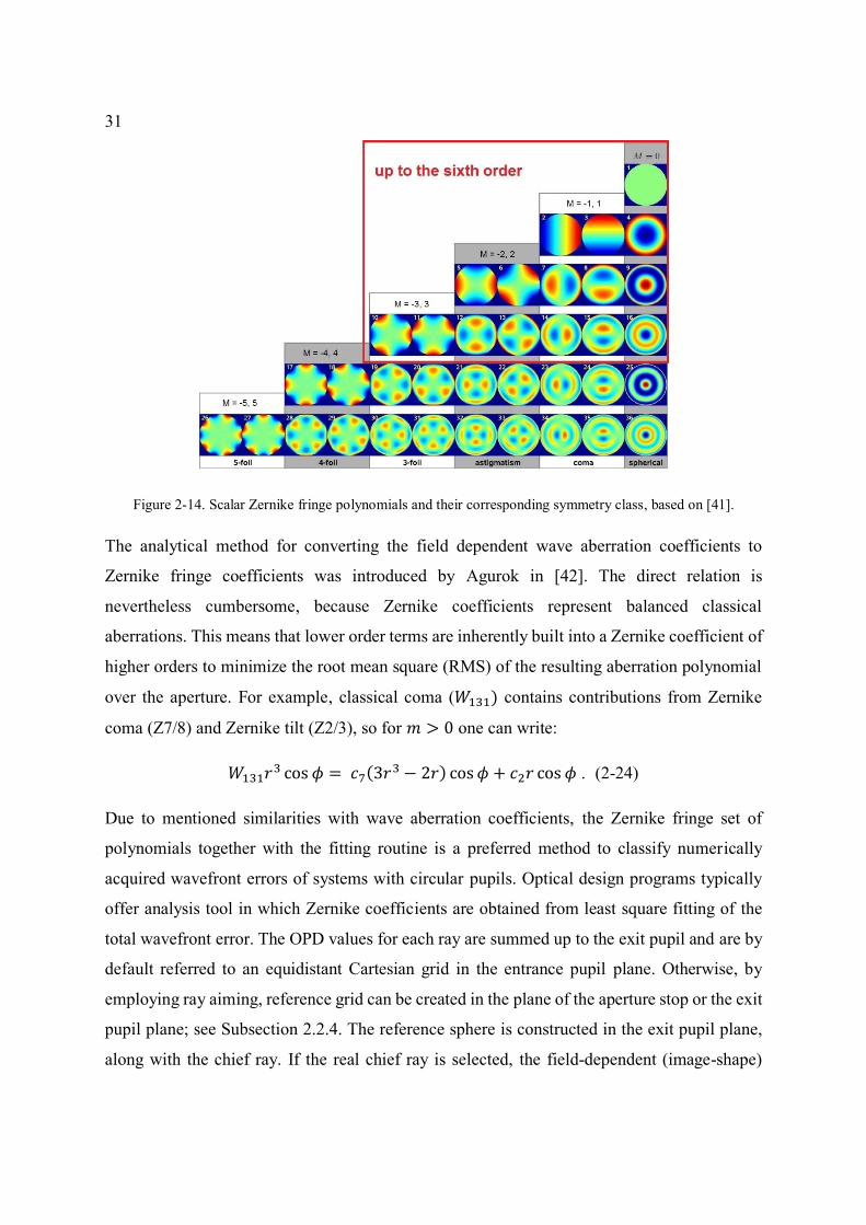
31
Figure 2-14. Scalar Zernike fringe polynomials and their corresponding symmetry class, based on [41].
The analytical method for converting the field dependent wave aberration coefficients to
Zernike fringe coefficients was introduced by Agurok in [42]. The direct relation is
nevertheless cumbersome, because Zernike coefficients represent balanced classical
aberrations. This means that lower order terms are inherently built into a Zernike coefficient of
higher orders to minimize the root mean square (RMS) of the resulting aberration polynomial
over the aperture. For example, classical coma (𝑊131) contains contributions from Zernike
coma (Z7/8) and Zernike tilt (Z2/3), so for 𝑚 > 0 one can write:
𝑊131𝑟3 cos 𝜙 = 𝑐7(3𝑟
3 − 2𝑟) cos 𝜙 + 𝑐2𝑟 cos 𝜙 . (2-24)
Due to mentioned similarities with wave aberration coefficients, the Zernike fringe set of
polynomials together with the fitting routine is a preferred method to classify numerically
acquired wavefront errors of systems with circular pupils. Optical design programs typically
offer analysis tool in which Zernike coefficients are obtained from least square fitting of the
total wavefront error. The OPD values for each ray are summed up to the exit pupil and are by
default referred to an equidistant Cartesian grid in the entrance pupil plane. Otherwise, by
employing ray aiming, reference grid can be created in the plane of the aperture stop or the exit
pupil plane; see Subsection 2.2.4. The reference sphere is constructed in the exit pupil plane,
along with the chief ray. If the real chief ray is selected, the field-dependent (image-shape)
32
aberrations are not included in the shape of the obtained wavefront error, therefore generally
one can write:
𝑊𝑡𝑜𝑡 (ρ𝑥, ρ𝑦) = ∑ 𝑐𝑖𝑍𝑖(ρ𝑥, ρ𝑦)𝑖 , (2-25)
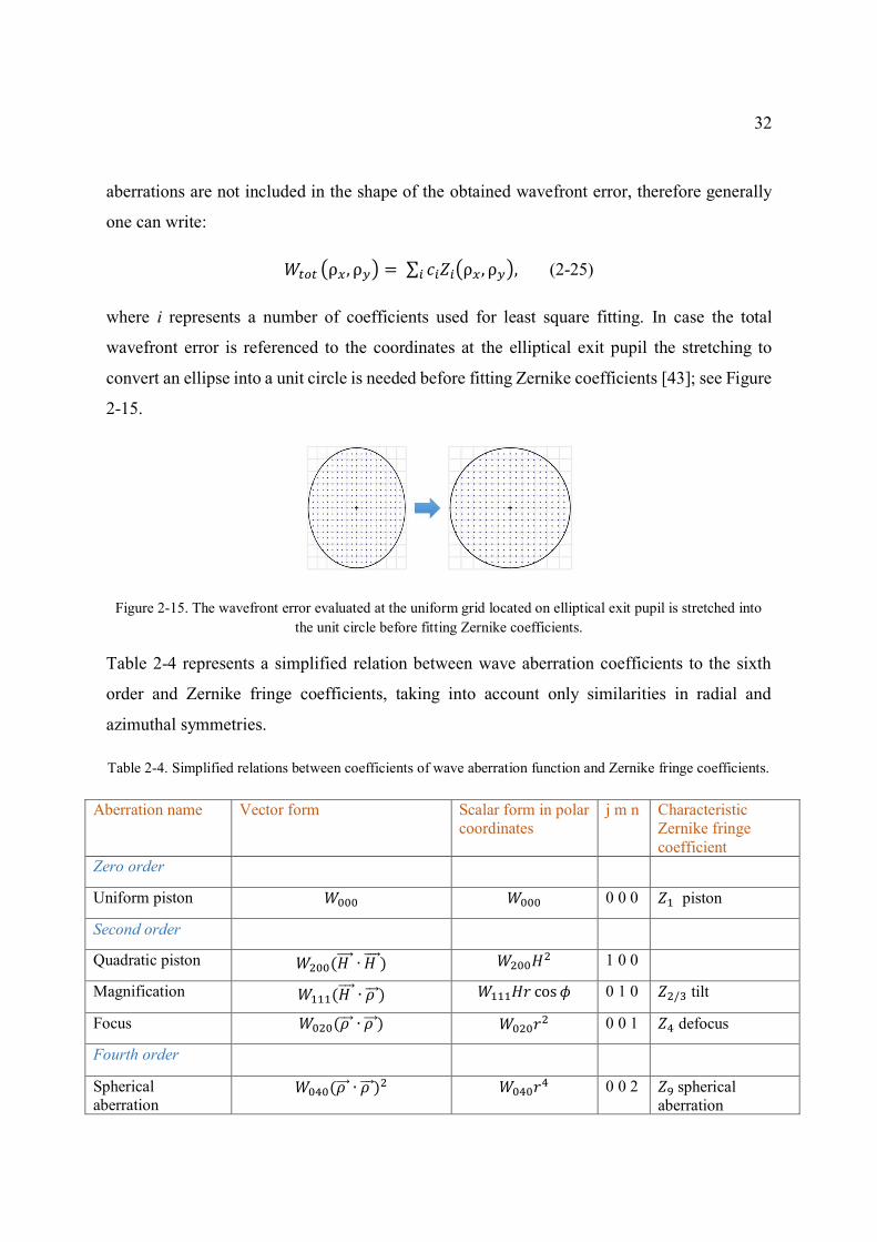
where i represents a number of coefficients used for least square fitting. In case the total
wavefront error is referenced to the coordinates at the elliptical exit pupil the stretching to
convert an ellipse into a unit circle is needed before fitting Zernike coefficients [43]; see Figure
2-15.
Figure 2-15. The wavefront error evaluated at the uniform grid located on elliptical exit pupil is stretched into
the unit circle before fitting Zernike coefficients.
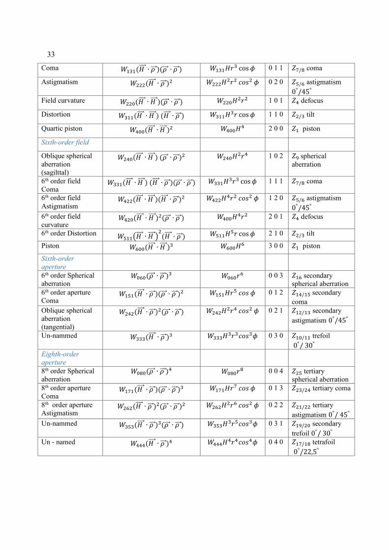
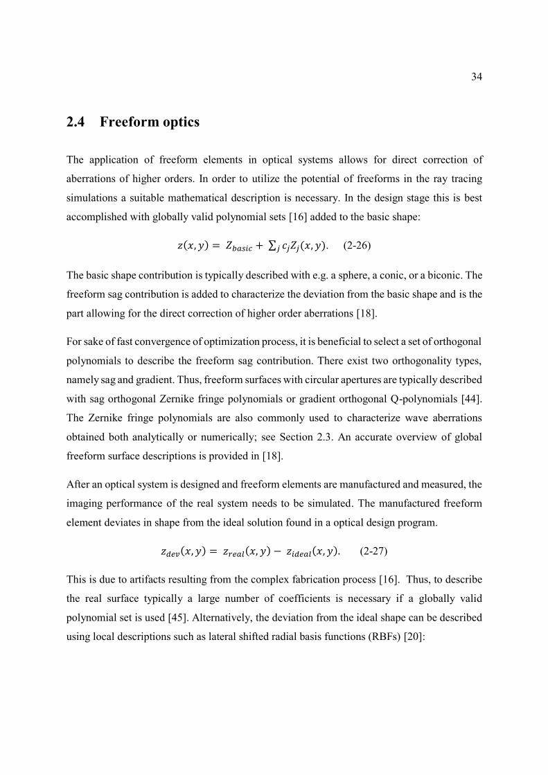
Table 2-4 represents a simplified relation between wave aberration coefficients to the sixth
order and Zernike fringe coefficients, taking into account only similarities in radial and
azimuthal symmetries.
Table 2-4. Simplified relations between coefficients of wave aberration function and Zernike fringe coefficients.
Aberration name Vector form Scalar form in polar
coordinates
j m n Characteristic
Zernike fringe
coefficient
Zero order
Uniform piston 𝑊000 𝑊000 0 0 0 𝑍1 piston
Second order
Quadratic piston 𝑊200(𝐻 ⃗⃗⃗⃗ ∙ 𝐻 ⃗⃗⃗⃗ ) 𝑊200𝐻2 1 0 0
Magnification 𝑊111(𝐻 ⃗⃗⃗⃗ ∙ 𝜌 ⃗⃗⃗ ) 𝑊111𝐻𝑟 cos𝜙 0 1 0 𝑍2/3 tilt
Focus 𝑊020(𝜌 ⃗⃗⃗ ∙ 𝜌 ⃗⃗⃗ ) 𝑊020𝑟2 0 0 1 𝑍4 defocus
Fourth order
Spherical
aberration 𝑊040(𝜌 ⃗⃗⃗ ∙ 𝜌 ⃗⃗⃗ )2 𝑊040𝑟
4 0 0 2 𝑍9 spherical
aberration
33
Coma 𝑊131(𝐻 ⃗⃗⃗⃗ ∙ 𝜌 ⃗⃗⃗ )(𝜌 ⃗⃗⃗ ∙ 𝜌 ⃗⃗⃗ ) 𝑊131𝐻𝑟3 cos𝜙 0 1 1 𝑍7/8 coma
Astigmatism 𝑊222(𝐻 ⃗⃗⃗⃗ ∙ 𝜌 ⃗⃗⃗ )2 𝑊222𝐻2𝑟2 𝑐𝑜𝑠2 𝜙 0 2 0 𝑍5/6 astigmatism
0°/45°
Field curvature 𝑊220(𝐻 ⃗⃗⃗⃗ ∙ 𝐻 ⃗⃗⃗⃗ )(𝜌 ⃗⃗⃗ ∙ 𝜌 ⃗⃗⃗ ) 𝑊220𝐻2𝑟2 1 0 1 𝑍4 defocus
Distortion 𝑊311(𝐻 ⃗⃗⃗⃗ ∙ 𝐻 ⃗⃗⃗⃗ ) (𝐻 ⃗⃗⃗⃗ ∙ 𝜌 ⃗⃗⃗ ) 𝑊311𝐻3𝑟 cos𝜙 1 1 0 𝑍2/3 tilt
Quartic piston 𝑊400(𝐻 ⃗⃗⃗⃗ ∙ 𝐻 ⃗⃗⃗⃗ )2 𝑊400𝐻4 2 0 0 𝑍1 piston
Sixth-order field
Oblique spherical
aberration
(sagilttal)
𝑊240(𝐻 ⃗⃗⃗⃗ ∙ 𝐻 ⃗⃗⃗⃗ ) (𝜌 ⃗⃗⃗ ∙ 𝜌 ⃗⃗⃗ )2 𝑊240𝐻2𝑟4 1 0 2 𝑍9 spherical
aberration
6th order field
Coma 𝑊331(𝐻 ⃗⃗⃗⃗ ∙ 𝐻 ⃗⃗⃗⃗ ) (𝐻 ⃗⃗⃗⃗ ∙ 𝜌 ⃗⃗⃗ )(𝜌 ⃗⃗⃗ ∙ 𝜌 ⃗⃗⃗ ) 𝑊331𝐻
3𝑟3 cos𝜙 1 1 1 𝑍7/8 coma
6th order field
Astigmatism 𝑊422(𝐻 ⃗⃗⃗⃗ ∙ 𝐻 ⃗⃗⃗⃗ )(𝐻 ⃗⃗⃗⃗ ∙ 𝜌 ⃗⃗⃗ )2 𝑊422𝐻
4𝑟2 𝑐𝑜𝑠2 𝜙 1 2 0 𝑍5/6 astigmatism
0°/45°
6th order field
curvature 𝑊420(𝐻 ⃗⃗⃗⃗ ∙ 𝐻 ⃗⃗⃗⃗ )2(𝜌 ⃗⃗⃗ ∙ 𝜌 ⃗⃗⃗ ) 𝑊400𝐻
4𝑟2 2 0 1 𝑍4 defocus
6th order Distortion 𝑊511(𝐻 ⃗⃗⃗⃗ ∙ 𝐻 ⃗⃗⃗⃗ )2(𝐻 ⃗⃗⃗⃗ ∙ 𝜌 ⃗⃗⃗ ) 𝑊511𝐻
5𝑟 cos𝜙 2 1 0 𝑍2/3 tilt
Piston 𝑊600(𝐻 ⃗⃗⃗⃗ ∙ 𝐻 ⃗⃗⃗⃗ )3 𝑊600𝐻6 3 0 0 𝑍1 piston
Sixth-order
aperture
6th order Spherical
aberration 𝑊060(𝜌 ⃗⃗⃗ ∙ 𝜌 ⃗⃗⃗ )3 𝑊060𝑟
6 0 0 3 𝑍16 secondary
spherical aberration
6th order aperture
Coma 𝑊151(𝐻 ⃗⃗⃗⃗ ∙ 𝜌 ⃗⃗⃗ )(𝜌 ⃗⃗⃗ ∙ 𝜌 ⃗⃗⃗ )2 𝑊151𝐻𝑟5 𝑐𝑜𝑠 𝜙 0 1 2 𝑍14/15 secondary
coma
Oblique spherical
aberration
(tangential)
𝑊242(𝐻 ⃗⃗⃗⃗ ∙ 𝜌 ⃗⃗⃗ )2(𝜌 ⃗⃗⃗ ∙ 𝜌 ⃗⃗⃗ ) 𝑊242𝐻2𝑟4 𝑐𝑜𝑠2 𝜙 0 2 1 𝑍12/13 secondary
astigmatism 0°/45°
Un-nammed 𝑊333(𝐻 ⃗⃗⃗⃗ ∙ 𝜌 ⃗⃗⃗ )3 𝑊333𝐻3𝑟3𝑐𝑜𝑠3𝜙 0 3 0 𝑍10/11 trefoil
0°/ 30°
Eighth-order
aperture
8th order Spherical
aberration 𝑊080(𝜌 ⃗⃗⃗ ∙ 𝜌 ⃗⃗⃗ )4 𝑊080𝑟
8 0 0 4 𝑍25 tertiary
spherical aberration
8th order aperture
Coma 𝑊171(𝐻 ⃗⃗⃗⃗ ∙ 𝜌 ⃗⃗⃗ )(𝜌 ⃗⃗⃗ ∙ 𝜌 ⃗⃗⃗ )3 𝑊171𝐻𝑟7 𝑐𝑜𝑠 𝜙 0 1 3 𝑍23/24 tertiary coma
8th order aperture
Astigmatism 𝑊262(𝐻 ⃗⃗⃗⃗ ∙ 𝜌 ⃗⃗⃗ )2(𝜌 ⃗⃗⃗ ∙ 𝜌 ⃗⃗⃗ )2 𝑊262𝐻
2𝑟6 𝑐𝑜𝑠2 𝜙 0 2 2 𝑍21/22 tertiary
astigmatism 0°/ 45°
Un-nammed 𝑊353(𝐻 ⃗⃗⃗⃗ ∙ 𝜌 ⃗⃗⃗ )3(𝜌 ⃗⃗⃗ ∙ 𝜌 ⃗⃗⃗ ) 𝑊353𝐻3𝑟5𝑐𝑜𝑠3𝜙 0 3 1 𝑍19/20 secondary
trefoil 0°/ 30°
Un - named 𝑊444(𝐻 ⃗⃗⃗⃗ ∙ 𝜌 ⃗⃗⃗ )4 𝑊444𝐻4𝑟4𝑐𝑜𝑠4𝜙 0 4 0 𝑍17/18 tetrafoil
0°/22,5°
34
2.4 Freeform optics
The application of freeform elements in optical systems allows for direct correction of
aberrations of higher orders. In order to utilize the potential of freeforms in the ray tracing
simulations a suitable mathematical description is necessary. In the design stage this is best
accomplished with globally valid polynomial sets [16] added to the basic shape:
𝑧(𝑥, 𝑦) = 𝑍𝑏𝑎𝑠𝑖𝑐 + ∑ 𝑐𝑗𝑍𝑗(𝑥, 𝑦)𝑗 . (2-26)
The basic shape contribution is typically described with e.g. a sphere, a conic, or a biconic. The
freeform sag contribution is added to characterize the deviation from the basic shape and is the
part allowing for the direct correction of higher order aberrations [18].
For sake of fast convergence of optimization process, it is beneficial to select a set of orthogonal
polynomials to describe the freeform sag contribution. There exist two orthogonality types,
namely sag and gradient. Thus, freeform surfaces with circular apertures are typically described
with sag orthogonal Zernike fringe polynomials or gradient orthogonal Q-polynomials [44].
The Zernike fringe polynomials are also commonly used to characterize wave aberrations
obtained both analytically or numerically; see Section 2.3. An accurate overview of global
freeform surface descriptions is provided in [18].
After an optical system is designed and freeform elements are manufactured and measured, the
imaging performance of the real system needs to be simulated. The manufactured freeform
element deviates in shape from the ideal solution found in a optical design program.
𝑧𝑑𝑒𝑣(𝑥, 𝑦) = 𝑧𝑟𝑒𝑎𝑙(𝑥, 𝑦) − 𝑧𝑖𝑑𝑒𝑎𝑙(𝑥, 𝑦). (2-27)
This is due to artifacts resulting from the complex fabrication process [16]. Thus, to describe
the real surface typically a large number of coefficients is necessary if a globally valid
polynomial set is used [45]. Alternatively, the deviation from the ideal shape can be described
using local descriptions such as lateral shifted radial basis functions (RBFs) [20]:
35
2.5 Tolerance sensitivity analysis
The imaging performance of a real system differs from that simulated in the optical design
program. Thus, for the real system to meet specifications tolerances need to be assigned after
the design stage. Tolerances are divided into two categories, namely manufacturing tolerances
and assembly tolerances. Further, with respect to system parameters the first group can be
divided into form and material tolerances and the later into decenter and tilt tolerances. To
determine values for each tolerance it is helpful to study the sensitivity of the system to changes
of these parameters. This is carried out by evaluating a change in a performance criterion 𝑏𝑗
with respect to a change of system parameter 𝑡𝑘 on surface 𝑘 [39]:
∆𝑏𝑗(𝑡𝑘) = 𝑏𝑗𝑖𝑑𝑒𝑎𝑙 − 𝑏𝑗(∆𝑡𝑘) . (2-28)
In this way only the effect of deviation of a single parameter is evaluated. However, during
manufacturing or assembling of a real system more than one parameter are typically perturbed.
Thus, to estimate the net effect the superposition of changes upon each perturbed system
parameter is used. There are three possible models:
𝑆𝑡𝑎𝑡𝑖𝑠𝑡𝑖𝑐𝑎𝑙 𝑠𝑢𝑝𝑒𝑟𝑝𝑜𝑠𝑖𝑡𝑖𝑜𝑛: ∆�̃�𝑗𝑠𝑡𝑎𝑡𝑖𝑠𝑡𝑖𝑐𝑎𝑙 = √∑ ∆𝑏𝑗(𝑡𝑘)2𝑘
𝐿𝑖𝑛𝑒𝑎𝑟 𝑠𝑢𝑝𝑒𝑟𝑝𝑜𝑠𝑖𝑡𝑖𝑜𝑛: ∆�̃�𝑗𝑙𝑖𝑛𝑒𝑎𝑟 = ∑ ∆𝑏𝑗(𝑡𝑘)𝑘 (2-29)
𝑊𝑜𝑟𝑠𝑡 − 𝑐𝑎𝑠𝑒 𝑠𝑢𝑝𝑒𝑟𝑝𝑜𝑠𝑖𝑡𝑖𝑜𝑛: ∆�̃�𝑗𝑤𝑜𝑟𝑠 𝑐𝑎𝑠𝑒 = ∑|∆𝑏𝑗(𝑡𝑘)|
𝑘
Further, in order to consider the varying azimuthal orientation of parameters the Räntsch
superposition model can be applied. This adjustment step is obtained with:
∆�̃�𝑗𝑅ä𝑛𝑡𝑠𝑐ℎ = √∆�̃�𝑗
𝑠𝑡𝑎𝑡𝑖𝑠𝑡𝑖𝑐𝑎𝑙 ∙ ∆�̃�𝑗𝑤𝑜𝑟𝑠 𝑐𝑎𝑠𝑒 . (2-30)
The sensitivity analysis is especially useful in estimating the assembly tolerances. The surface
with the most significant influence on the imaging performance can be identified and used as
a compensator in the alignment process of the system.
The sensitivity analysis based on the performance of perturbed systems is computationally
intensive and is carried out after the design stage. However, some insights about the “as-built”,
performance of a system can be gained priori, e.g. by studying aberrations generated in the
36
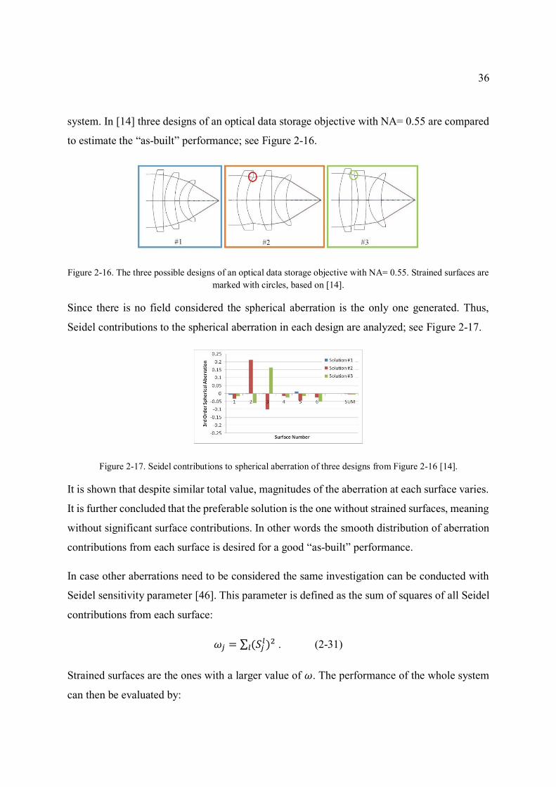
system. In [14] three designs of an optical data storage objective with NA= 0.55 are compared
to estimate the “as-built” performance; see Figure 2-16.
Figure 2-16. The three possible designs of an optical data storage objective with NA= 0.55. Strained surfaces are
marked with circles, based on [14].
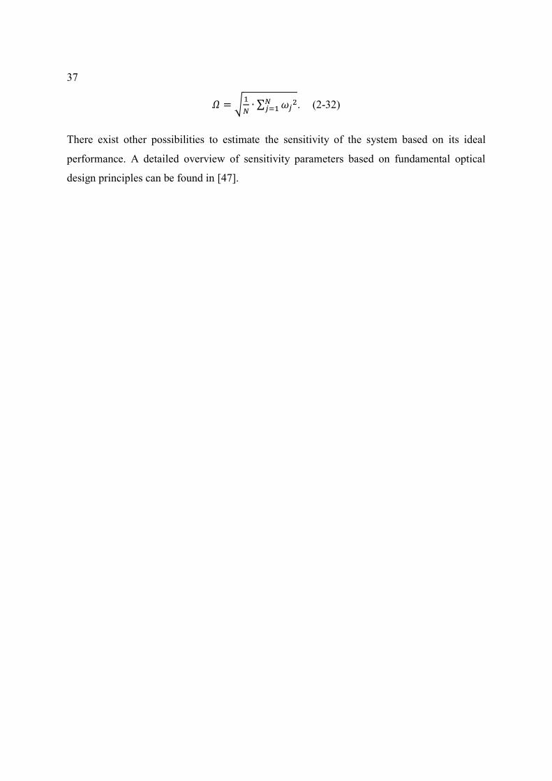
Since there is no field considered the spherical aberration is the only one generated. Thus,
Seidel contributions to the spherical aberration in each design are analyzed; see Figure 2-17.
Figure 2-17. Seidel contributions to spherical aberration of three designs from Figure 2-16 [14].
It is shown that despite similar total value, magnitudes of the aberration at each surface varies.
It is further concluded that the preferable solution is the one without strained surfaces, meaning
without significant surface contributions. In other words the smooth distribution of aberration
contributions from each surface is desired for a good “as-built” performance.
In case other aberrations need to be considered the same investigation can be conducted with
Seidel sensitivity parameter [46]. This parameter is defined as the sum of squares of all Seidel
contributions from each surface:
𝜔𝑗 = ∑ (𝑆𝑗𝑙)2𝑙 . (2-31)
Strained surfaces are the ones with a larger value of 𝜔. The performance of the whole system
can then be evaluated by:
37
𝛺 = √1
𝑁∙ ∑ 𝜔𝑗
2𝑁𝑗=1 . (2-32)
There exist other possibilities to estimate the sensitivity of the system based on its ideal
performance. A detailed overview of sensitivity parameters based on fundamental optical
design principles can be found in [47].
38
Chapter 3 Novel method for decomposition of
the total wave aberration
In the design process, surface-by-surface aberration contributions are of special interest. The
expansion of the wave aberration function into the field- and pupil-dependent coefficients is an
analytical method used for that purpose; see Section 2.1. In the following chapter, an alternative
numerical method utilizing data from the trace of multiple ray sets is described [48]. Surface
contributions are divided with respect to their phenomenological origin into intrinsic, induced
and transfer components. Each component is determined from a separate set of rays.
3.1 Intermediate references
As specified in the former chapter the convention chosen in this thesis is that the field vector
is placed at the object plane and the pupil vector is placed at the exit pupil reference sphere
defined individually for each field point. In the following section, a set of intermediate
references necessary to evaluate surface aberration contributions, is defined.
3.1.1 Reference spheres
The optical system is divided into segments of the optical path measured along the real chief
ray (RCR); see Subsection 2.2.2. Each segment covers one surface and a distance to a
subsequent surface. Surface contributions represent the change of a wavefront that occurs due
to propagation through individual segments. Thus, to evaluate surface contributions, reference
spheres are established directly at the intersection of the RCR with individual surfaces; see
Figure 3-1. Each segment is therefore bounded with an entrance sphere before a surface and an
exit sphere before a subsequent surface.
39
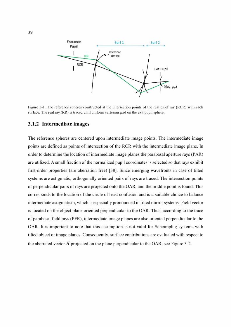
Figure 3-1. The reference spheres constructed at the intersection points of the real chief ray (RCR) with each
surface. The real ray (RR) is traced until uniform cartesian grid on the exit pupil sphere.
3.1.2 Intermediate images
The reference spheres are centered upon intermediate image points. The intermediate image
points are defined as points of intersection of the RCR with the intermediate image plane. In
order to determine the location of intermediate image planes the parabasal aperture rays (PAR)
are utilized. A small fraction of the normalized pupil coordinates is selected so that rays exhibit
first-order properties (are aberration free) [38]. Since emerging wavefronts in case of tilted
systems are astigmatic, orthogonally oriented pairs of rays are traced. The intersection points
of perpendicular pairs of rays are projected onto the OAR, and the middle point is found. This
corresponds to the location of the circle of least confusion and is a suitable choice to balance
intermediate astigmatism, which is especially pronounced in tilted mirror systems. Field vector
is located on the object plane oriented perpendicular to the OAR. Thus, according to the trace
of parabasal field rays (PFR), intermediate image planes are also oriented perpendicular to the
OAR. It is important to note that this assumption is not valid for Scheimplug systems with
tilted object or image planes. Consequently, surface contributions are evaluated with respect to
the aberrated vector �⃗⃗� projected on the plane perpendicular to the OAR; see Figure 3-2.
40
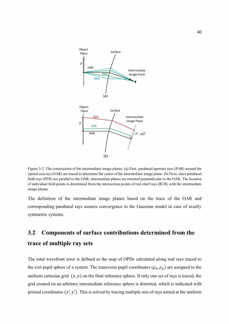
Figure 3-2. The construction of the intermediate image planes. (a) First, parabasal aperture rays (PAR) around the
optical axis ray (OAR) are traced to determine the center of the intermediate image plane. (b) Next, since parabasal
field rays (PFR) are parallel to the OAR, intermediate planes are oriented perpendicular to the OAR. The location
of individual field points is determined from the intersection points of real chief rays (RCR) with the intermediate
image planes.
The definition of the intermediate image planes based on the trace of the OAR and
corresponding parabasal rays assures convergence to the Gaussian model in case of axially
symmetric systems.
3.2 Components of surface contributions determined from the
trace of multiple ray sets
The total wavefront error is defined as the map of OPDs calculated along real rays traced to
the exit pupil sphere of a system. The transverse pupil coordinates (𝜌𝑥, 𝜌𝑦) are assigned to the
uniform cartesian grid (𝑥, 𝑦) on the final reference sphere. If only one set of rays is traced, the
grid created on an arbitrary intermediate reference sphere is distorted, which is indicated with
primed coordinates (𝑥′, 𝑦′). This is solved by tracing multiple sets of rays aimed at the uniform
41
grids (𝑥, 𝑦) of local coordinates on each reference sphere. Consequently, instead of measuring
the OPD along a single real ray up to the exit pupil sphere, multiple rays are used. This can be
thought of as evaluating wavefront errors after each surface at the similar undistorted set of
coordinates on reference spheres. Thus, wavefront errors can be subtracted from each other to
find the change caused by a particular segment of a system. This is explained for the single
OPD value in Figure 3-3.
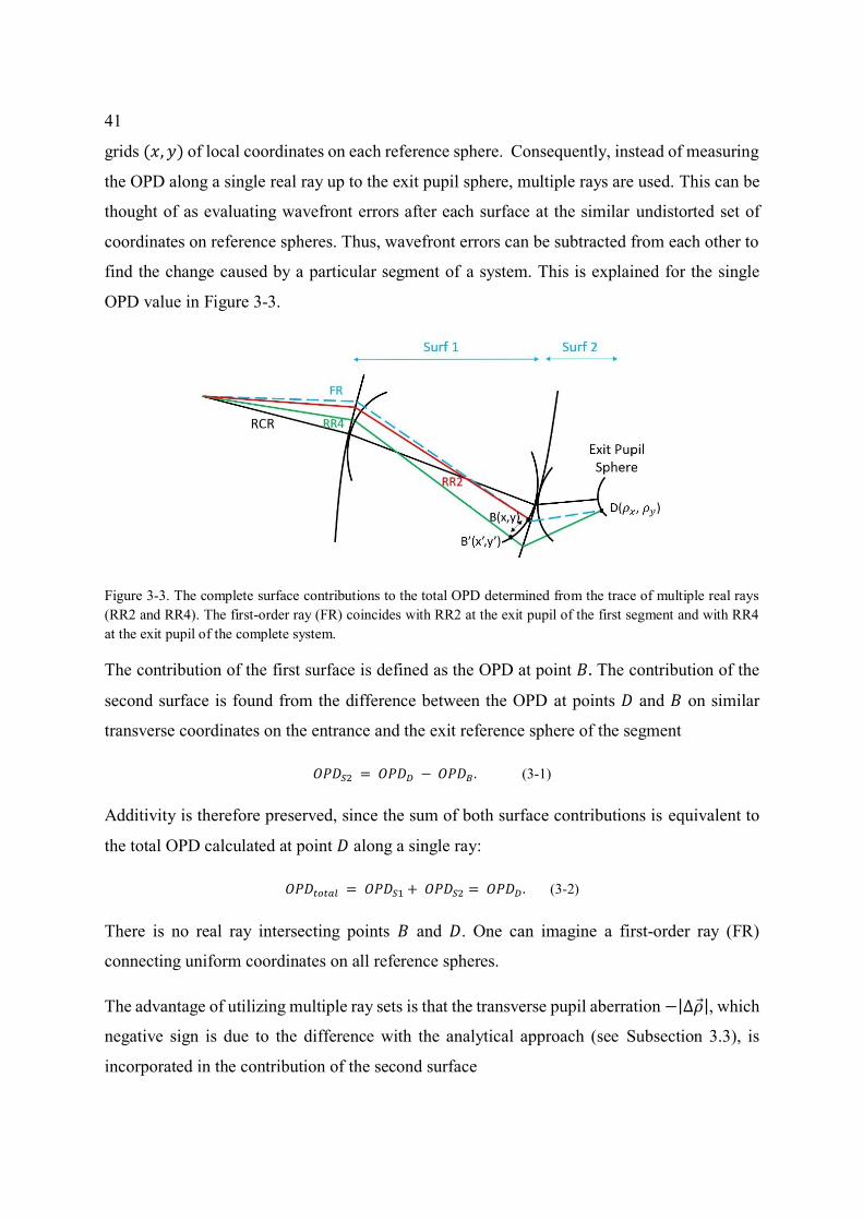
Figure 3-3. The complete surface contributions to the total OPD determined from the trace of multiple real rays
(RR2 and RR4). The first-order ray (FR) coincides with RR2 at the exit pupil of the first segment and with RR4
at the exit pupil of the complete system.
The contribution of the first surface is defined as the OPD at point 𝐵. The contribution of the
second surface is found from the difference between the OPD at points 𝐷 and 𝐵 on similar
transverse coordinates on the entrance and the exit reference sphere of the segment
𝑂𝑃𝐷𝑆2 = 𝑂𝑃𝐷𝐷 − 𝑂𝑃𝐷𝐵 . (3-1)
Additivity is therefore preserved, since the sum of both surface contributions is equivalent to
the total OPD calculated at point 𝐷 along a single ray:
𝑂𝑃𝐷𝑡𝑜𝑡𝑎𝑙 = 𝑂𝑃𝐷𝑆1 + 𝑂𝑃𝐷𝑆2 = 𝑂𝑃𝐷𝐷 . (3-2)
There is no real ray intersecting points 𝐵 and 𝐷. One can imagine a first-order ray (FR)
connecting uniform coordinates on all reference spheres.
The advantage of utilizing multiple ray sets is that the transverse pupil aberration −|∆𝜌 |, which
negative sign is due to the difference with the analytical approach (see Subsection 3.3), is
incorporated in the contribution of the second surface
42
−|∆𝜌 | = [(𝐵′𝑥 − 𝐵𝑥), (𝐵′𝑦 − 𝐵𝑦) ]. (3-3)
This allows for extraction of the induced effect defined here as a result of incoming aberrations
and the pupil distortion. Thus, the surface contribution is further divided into the intrinsic and
induced parts resulting from refraction on the surface and the transfer component, which is
present due to the propagation of the aberrated wavefront in free space.
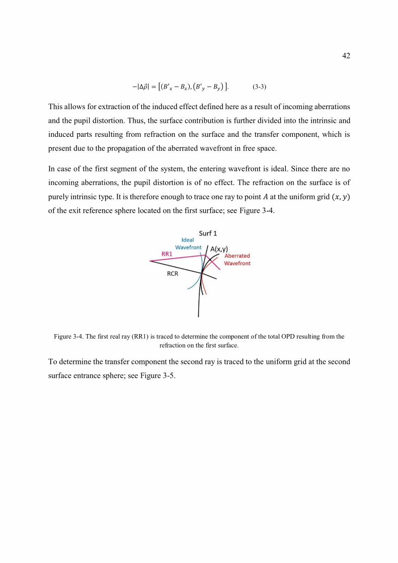
In case of the first segment of the system, the entering wavefront is ideal. Since there are no
incoming aberrations, the pupil distortion is of no effect. The refraction on the surface is of
purely intrinsic type. It is therefore enough to trace one ray to point 𝐴 at the uniform grid (𝑥, 𝑦)
of the exit reference sphere located on the first surface; see Figure 3-4.
Figure 3-4. The first real ray (RR1) is traced to determine the component of the total OPD resulting from the
refraction on the first surface.
To determine the transfer component the second ray is traced to the uniform grid at the second
surface entrance sphere; see Figure 3-5.
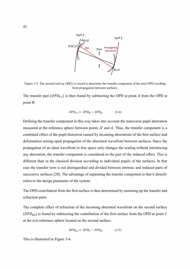
43
Figure 3-5. The second real ray (RR2) is traced to determine the transfer component of the total OPD resulting
from propagation between surfaces.
The transfer part (𝑂𝑃𝐷𝑇1) is then found by subtracting the OPD at point 𝐴 from the OPD at
point 𝐵:
𝑂𝑃𝐷𝑇1 = 𝑂𝑃𝐷𝐵 − 𝑂𝑃𝐷𝐴. (3-4)
Defining the transfer component in this way takes into account the transverse pupil aberration
measured at the reference sphere between points 𝐴′ and 𝐴. Thus, the transfer component is a
combined effect of the pupil distortion caused by incoming aberrations of the first surface and
deformation arising upon propagation of the aberrated wavefront between surfaces. Since the
propagation of an ideal wavefront in free space only changes the scaling without introducing
any aberration, the transfer component is considered as the part of the induced effect. This is
different than in the classical division according to individual pupils of the surfaces. In that
case the transfer term is not distinguished and divided between intrinsic and induced parts of
successive surfaces [28]. The advantage of separating the transfer component is that it directly
refers to the design parameter of the system.
The OPD contribution from the first surface is then determined by summing up the transfer and
refraction parts.
The complete effect of refraction of the incoming aberrated wavefront on the second surface
(𝑂𝑃𝐷𝑅2) is found by subtracting the contribution of the first surface from the OPD at point 𝐶
at the exit reference sphere located on the second surface:
𝑂𝑃𝐷𝑅2 = 𝑂𝑃𝐷𝐶 − 𝑂𝑃𝐷𝐵. (3-5)
This is illustrated in Figure 3-6.
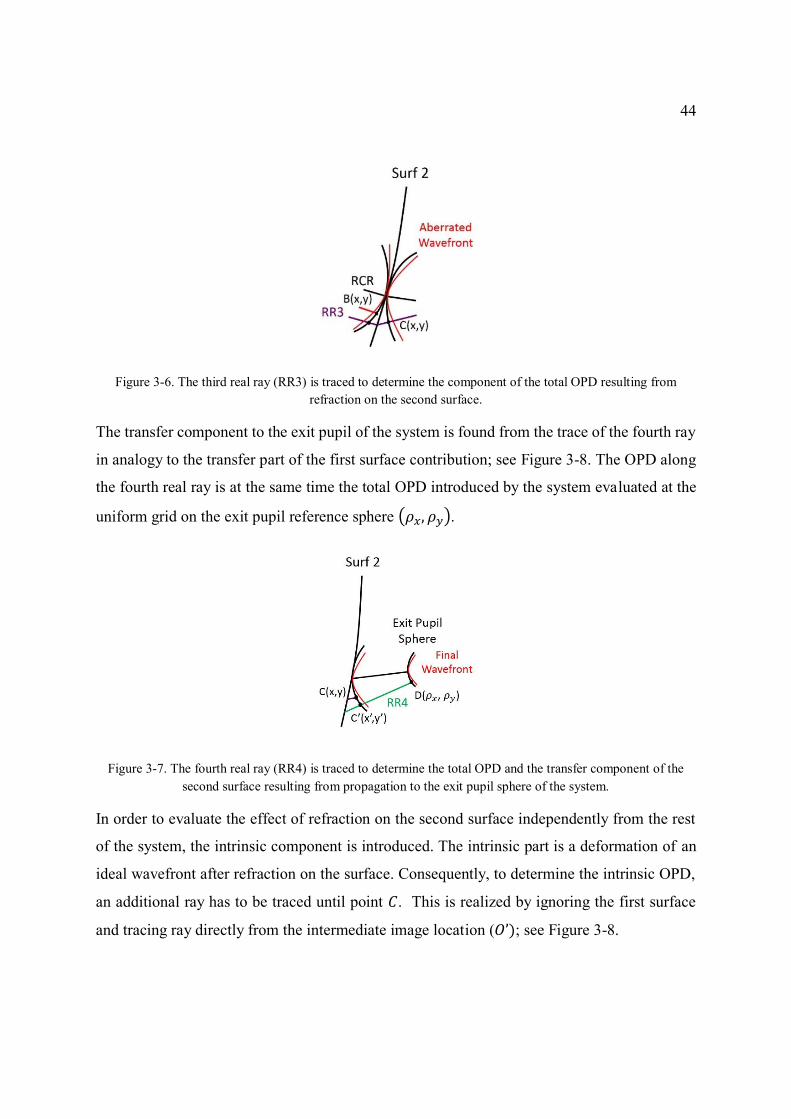
44
Figure 3-6. The third real ray (RR3) is traced to determine the component of the total OPD resulting from
refraction on the second surface.
The transfer component to the exit pupil of the system is found from the trace of the fourth ray
in analogy to the transfer part of the first surface contribution; see Figure 3-8. The OPD along
the fourth real ray is at the same time the total OPD introduced by the system evaluated at the
uniform grid on the exit pupil reference sphere (𝜌𝑥, 𝜌𝑦).
Figure 3-7. The fourth real ray (RR4) is traced to determine the total OPD and the transfer component of the
second surface resulting from propagation to the exit pupil sphere of the system.
In order to evaluate the effect of refraction on the second surface independently from the rest
of the system, the intrinsic component is introduced. The intrinsic part is a deformation of an
ideal wavefront after refraction on the surface. Consequently, to determine the intrinsic OPD,
an additional ray has to be traced until point 𝐶. This is realized by ignoring the first surface
and tracing ray directly from the intermediate image location (𝑂’); see Figure 3-8.
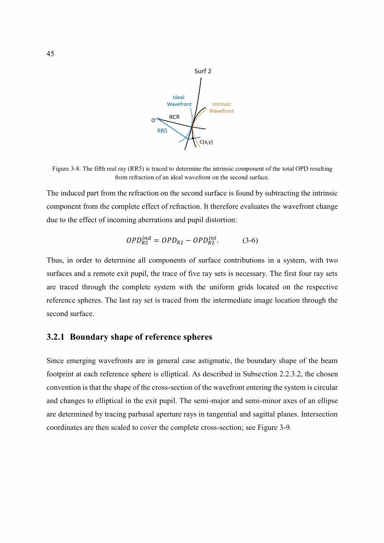
45
Figure 3-8. The fifth real ray (RR5) is traced to determine the intrinsic component of the total OPD resulting
from refraction of an ideal wavefront on the second surface.
The induced part from the refraction on the second surface is found by subtracting the intrinsic
component from the complete effect of refraction. It therefore evaluates the wavefront change
due to the effect of incoming aberrations and pupil distortion:
𝑂𝑃𝐷𝑅2𝑖𝑛𝑑 = 𝑂𝑃𝐷𝑅2 − 𝑂𝑃𝐷𝑅2
𝑖𝑛𝑡. (3-6)
Thus, in order to determine all components of surface contributions in a system, with two
surfaces and a remote exit pupil, the trace of five ray sets is necessary. The first four ray sets
are traced through the complete system with the uniform grids located on the respective
reference spheres. The last ray set is traced from the intermediate image location through the
second surface.
3.2.1 Boundary shape of reference spheres
Since emerging wavefronts are in general case astigmatic, the boundary shape of the beam
footprint at each reference sphere is elliptical. As described in Subsection 2.2.3.2, the chosen
convention is that the shape of the cross-section of the wavefront entering the system is circular
and changes to elliptical in the exit pupil. The semi-major and semi-minor axes of an ellipse
are determined by tracing parbasal aperture rays in tangential and sagittal planes. Intersection
coordinates are then scaled to cover the complete cross-section; see Figure 3-9.
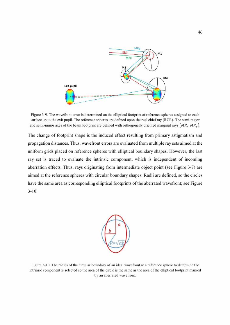
46
Figure 3-9. The wavefront error is determined on the elliptical footprint at reference spheres assigned to each
surface up to the exit pupil. The reference spheres are defined upon the real chief ray (RCR). The semi-major
and semi-minor axes of the beam footprint are defined with orthogonally oriented marginal rays (𝑀𝑅𝑥 ,𝑀𝑅𝑦).
The change of footprint shape is the induced effect resulting from primary astigmatism and
propagation distances. Thus, wavefront errors are evaluated from multiple ray sets aimed at the
uniform grids placed on reference spheres with elliptical boundary shapes. However, the last
ray set is traced to evaluate the intrinsic component, which is independent of incoming
aberration effects. Thus, rays originating from intermediate object point (see Figure 3-7) are
aimed at the reference spheres with circular boundary shapes. Radii are defined, so the circles
have the same area as corresponding elliptical footprints of the aberrated wavefront; see Figure
3-10.
Figure 3-10. The radius of the circular boundary of an ideal wavefront at a reference sphere to determine the
intrinsic component is selected so the area of the circle is the same as the area of the elliptical footprint marked
by an aberrated wavefront.
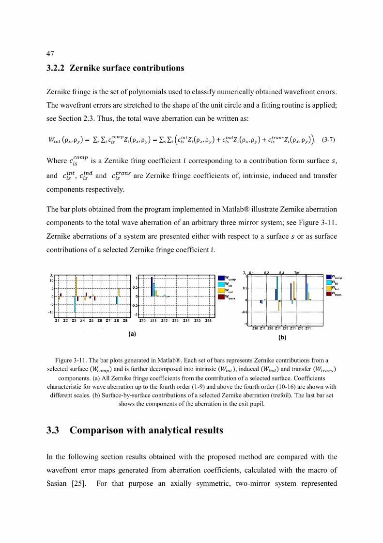
47
3.2.2 Zernike surface contributions
Zernike fringe is the set of polynomials used to classify numerically obtained wavefront errors.
The wavefront errors are stretched to the shape of the unit circle and a fitting routine is applied;
see Section 2.3. Thus, the total wave aberration can be written as:
𝑊𝑡𝑜𝑡 (ρ𝑥 , ρ𝑦) = ∑ ∑ 𝑐𝑖𝑠𝑐𝑜𝑚𝑝
𝑍𝑖(ρ𝑥 , ρ𝑦)𝑖𝑠 = ∑ ∑ (𝑐𝑖𝑠𝑖𝑛𝑡𝑍𝑖(ρ𝑥 , ρ𝑦) + 𝑐𝑖𝑠
𝑖𝑛𝑑𝑍𝑖(ρ𝑥 , ρ𝑦) + 𝑐𝑖𝑠𝑡𝑟𝑎𝑛𝑠𝑍𝑖(ρ𝑥 , ρ𝑦))𝑖𝑠 , (3-7)
Where 𝑐𝑖𝑠𝑐𝑜𝑚𝑝
is a Zernike fring coefficient 𝑖 corresponding to a contribution form surface 𝑠,
and 𝑐𝑖𝑠𝑖𝑛𝑡, 𝑐𝑖𝑠
𝑖𝑛𝑑 and 𝑐𝑖𝑠𝑡𝑟𝑎𝑛𝑠 are Zernike fringe coefficients of, intrinsic, induced and transfer
components respectively.
The bar plots obtained from the program implemented in Matlab® illustrate Zernike aberration
components to the total wave aberration of an arbitrary three mirror system; see Figure 3-11.
Zernike aberrations of a system are presented either with respect to a surface 𝑠 or as surface
contributions of a selected Zernike fringe coefficient 𝑖.
Figure 3-11. The bar plots generated in Matlab®. Each set of bars represents Zernike contributions from a
selected surface (𝑊𝑐𝑜𝑚𝑝) and is further decomposed into intrinsic (𝑊𝑖𝑛𝑡), induced (𝑊𝑖𝑛𝑑) and transfer (𝑊𝑡𝑟𝑎𝑛𝑠)
components. (a) All Zernike fringe coefficients from the contribution of a selected surface. Coefficients
characteristic for wave aberration up to the fourth order (1-9) and above the fourth order (10-16) are shown with
different scales. (b) Surface-by-surface contributions of a selected Zernike aberration (trefoil). The last bar set
shows the components of the aberration in the exit pupil.
3.3 Comparison with analytical results
In the following section results obtained with the proposed method are compared with the
wavefront error maps generated from aberration coefficients, calculated with the macro of
Sasian [25]. For that purpose an axially symmetric, two-mirror system represented
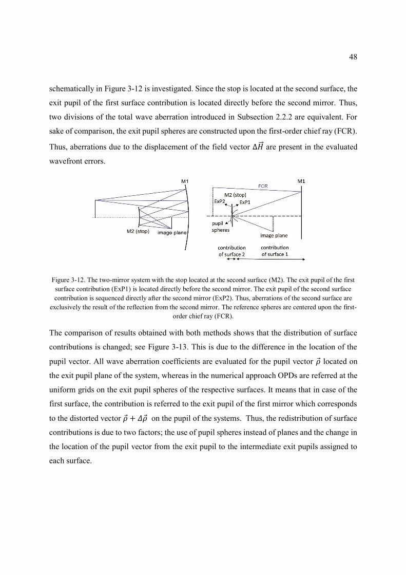
48
schematically in Figure 3-12 is investigated. Since the stop is located at the second surface, the
exit pupil of the first surface contribution is located directly before the second mirror. Thus,
two divisions of the total wave aberration introduced in Subsection 2.2.2 are equivalent. For
sake of comparison, the exit pupil spheres are constructed upon the first-order chief ray (FCR).
Thus, aberrations due to the displacement of the field vector ∆�⃗⃗� are present in the evaluated
wavefront errors.
Figure 3-12. The two-mirror system with the stop located at the second surface (M2). The exit pupil of the first
surface contribution (ExP1) is located directly before the second mirror. The exit pupil of the second surface
contribution is sequenced directly after the second mirror (ExP2). Thus, aberrations of the second surface are
exclusively the result of the reflection from the second mirror. The reference spheres are centered upon the first-
order chief ray (FCR).
The comparison of results obtained with both methods shows that the distribution of surface
contributions is changed; see Figure 3-13. This is due to the difference in the location of the
pupil vector. All wave aberration coefficients are evaluated for the pupil vector 𝜌 located on
the exit pupil plane of the system, whereas in the numerical approach OPDs are referred at the
uniform grids on the exit pupil spheres of the respective surfaces. It means that in case of the
first surface, the contribution is referred to the exit pupil of the first mirror which corresponds
to the distorted vector 𝜌 + 𝛥𝜌 on the pupil of the systems. Thus, the redistribution of surface
contributions is due to two factors; the use of pupil spheres instead of planes and the change in
the location of the pupil vector from the exit pupil to the intermediate exit pupils assigned to
each surface.
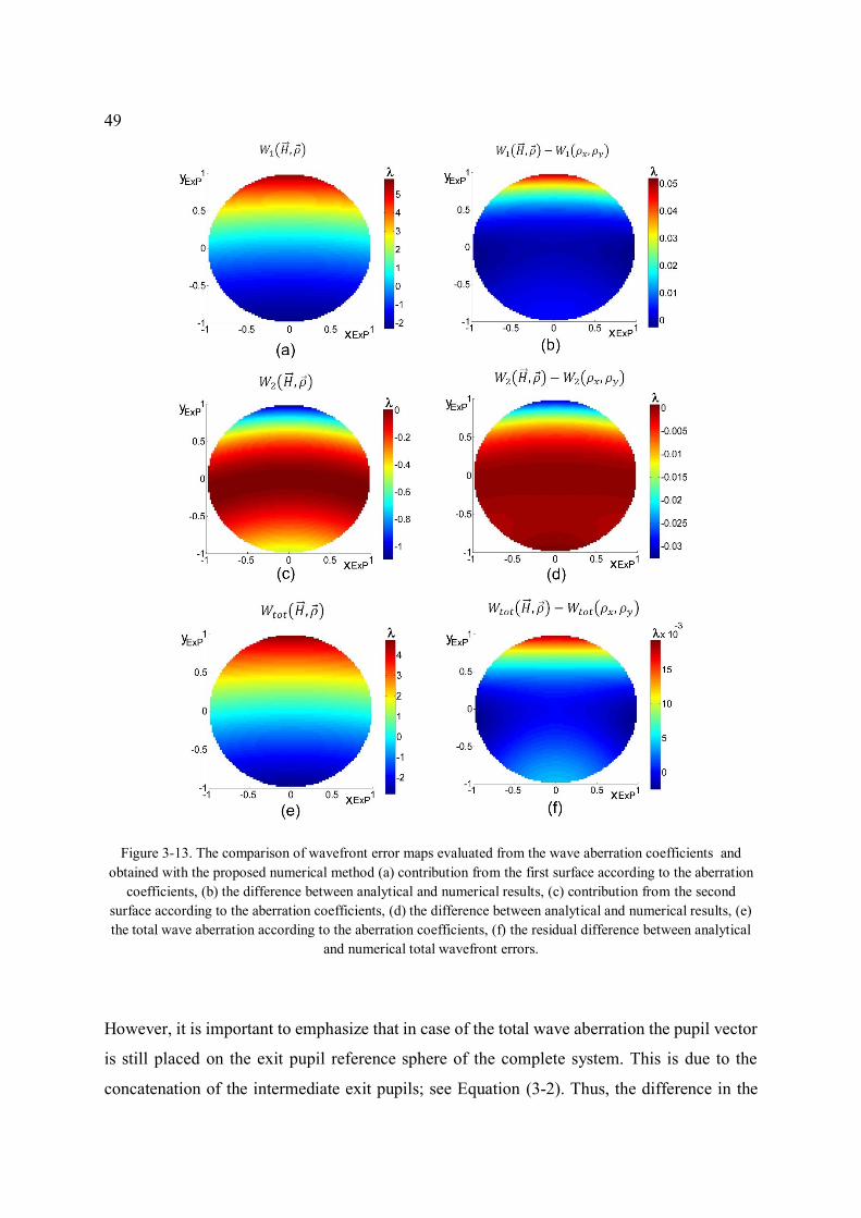
49
Figure 3-13. The comparison of wavefront error maps evaluated from the wave aberration coefficients and
obtained with the proposed numerical method (a) contribution from the first surface according to the aberration
coefficients, (b) the difference between analytical and numerical results, (c) contribution from the second
surface according to the aberration coefficients, (d) the difference between analytical and numerical results, (e)
the total wave aberration according to the aberration coefficients, (f) the residual difference between analytical
and numerical total wavefront errors.
However, it is important to emphasize that in case of the total wave aberration the pupil vector
is still placed on the exit pupil reference sphere of the complete system. This is due to the
concatenation of the intermediate exit pupils; see Equation (3-2). Thus, the difference in the
50
total wave aberration is only due to the change in the pupil shape, which is of less significance
as shown in Figure 3-13(f).
The redistribution of the surface contributions due to the different position of the equidistant
pupil grid, results in the sign difference of the induced component. As described in Subsection
2.1.5, in [29] the induced part of the second surface up to the sixth order depends on the fourth-
order incoming aberrations and the third-order transverse pupil aberration of the first surface,
measured with respect to the exit pupil of the system; see Equation (2-9).
Analogously, in case of the example system, for the numerical approach the induced part of
the second surface contribution with no restriction to the expansion order can be noted by:
𝑊2(𝑖𝑛𝑑)(�⃗⃗� , 𝜌 ) = (𝑊𝑡𝑜𝑡(�⃗⃗� , 𝜌 ) − 𝑊1(�⃗⃗� , 𝜌 + ∆𝜌 )) − 𝑊2
(𝑖𝑛𝑡)(�⃗⃗� , 𝜌 ). (3-8)
The term in the parenthesis is the complete contribution of the second surface defined as in the
Equation (3-1). The transverse pupil aberration is included with a different subtraction order
than in Equation (2-9). The same sign difference was indicated while deriving the transverse
pupil aberration in Equation (3-3). The further difference between both induced parts is due to
the transverse pupil aberration evaluated numerically on a sphere and analytically on a plane;
see Figure 3-14.
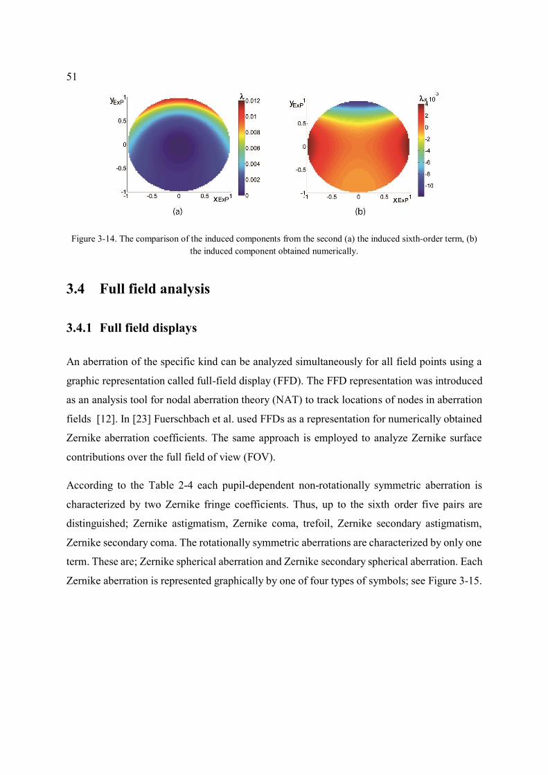
51
Figure 3-14. The comparison of the induced components from the second (a) the induced sixth-order term, (b)
the induced component obtained numerically.
3.4 Full field analysis
3.4.1 Full field displays
An aberration of the specific kind can be analyzed simultaneously for all field points using a
graphic representation called full-field display (FFD). The FFD representation was introduced
as an analysis tool for nodal aberration theory (NAT) to track locations of nodes in aberration
fields [12]. In [23] Fuerschbach et al. used FFDs as a representation for numerically obtained
Zernike aberration coefficients. The same approach is employed to analyze Zernike surface
contributions over the full field of view (FOV).
According to the Table 2-4 each pupil-dependent non-rotationally symmetric aberration is
characterized by two Zernike fringe coefficients. Thus, up to the sixth order five pairs are
distinguished; Zernike astigmatism, Zernike coma, trefoil, Zernike secondary astigmatism,
Zernike secondary coma. The rotationally symmetric aberrations are characterized by only one
term. These are; Zernike spherical aberration and Zernike secondary spherical aberration. Each
Zernike aberration is represented graphically by one of four types of symbols; see Figure 3-15.
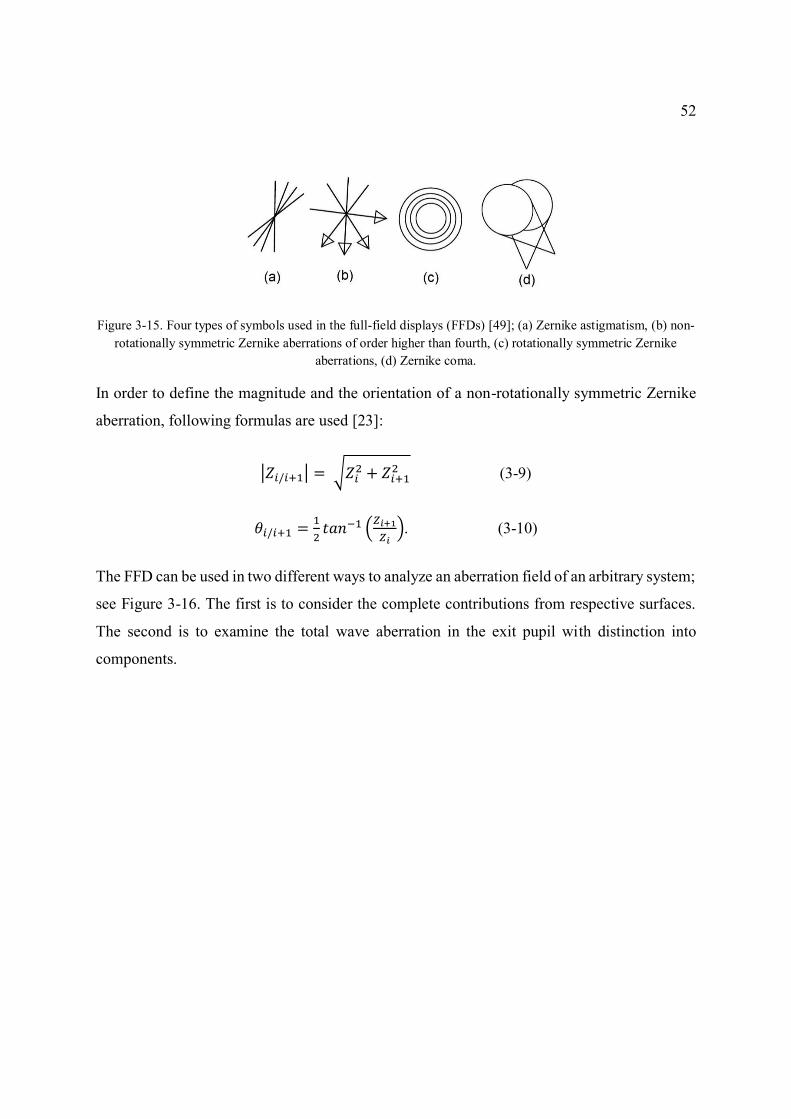
52
Figure 3-15. Four types of symbols used in the full-field displays (FFDs) [49]; (a) Zernike astigmatism, (b) non-
rotationally symmetric Zernike aberrations of order higher than fourth, (c) rotationally symmetric Zernike
aberrations, (d) Zernike coma.
In order to define the magnitude and the orientation of a non-rotationally symmetric Zernike
aberration, following formulas are used [23]:
|𝑍𝑖/𝑖+1| = √𝑍𝑖2 + 𝑍𝑖+1
2 (3-9)
𝜃𝑖/𝑖+1 =1
2𝑡𝑎𝑛−1 (
𝑍𝑖+1
𝑍𝑖). (3-10)
The FFD can be used in two different ways to analyze an aberration field of an arbitrary system;
see Figure 3-16. The first is to consider the complete contributions from respective surfaces.
The second is to examine the total wave aberration in the exit pupil with distinction into
components.
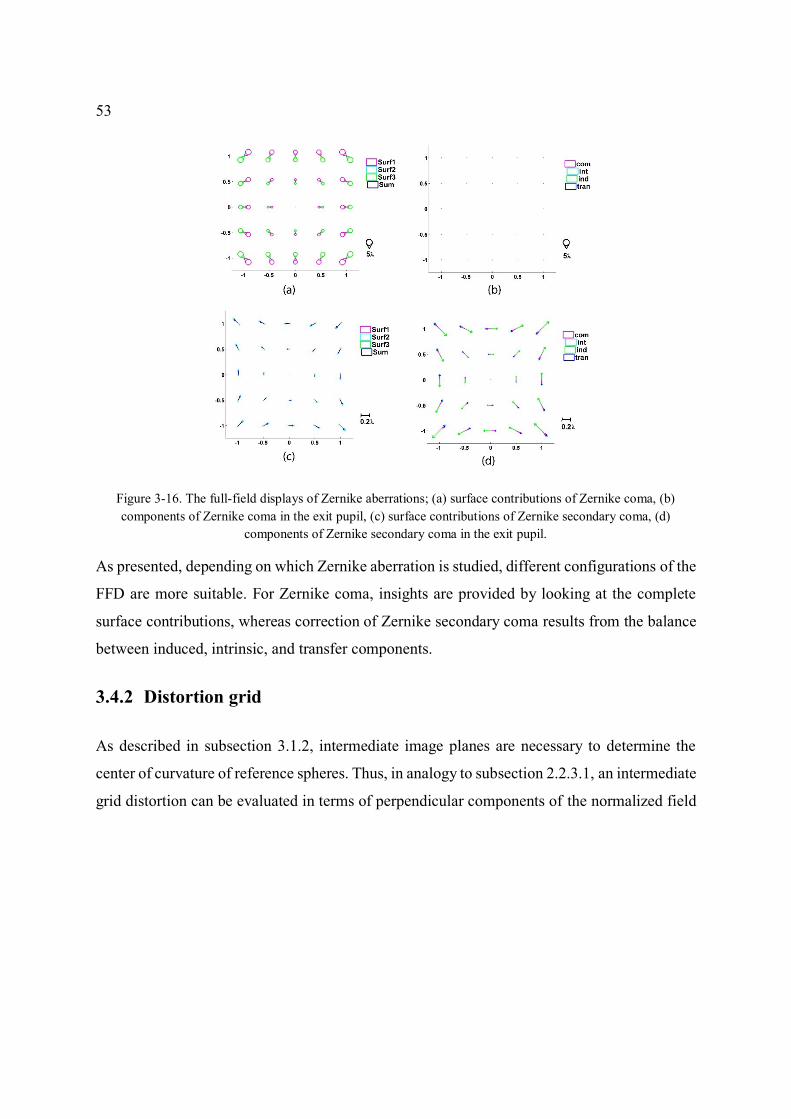
53
Figure 3-16. The full-field displays of Zernike aberrations; (a) surface contributions of Zernike coma, (b)
components of Zernike coma in the exit pupil, (c) surface contributions of Zernike secondary coma, (d)
components of Zernike secondary coma in the exit pupil.
As presented, depending on which Zernike aberration is studied, different configurations of the
FFD are more suitable. For Zernike coma, insights are provided by looking at the complete
surface contributions, whereas correction of Zernike secondary coma results from the balance
between induced, intrinsic, and transfer components.
3.4.2 Distortion grid
As described in subsection 3.1.2, intermediate image planes are necessary to determine the
center of curvature of reference spheres. Thus, in analogy to subsection 2.2.3.1, an intermediate
grid distortion can be evaluated in terms of perpendicular components of the normalized field
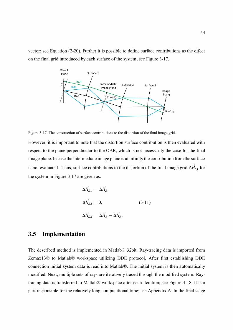
54
vector; see Equation (2-20). Further it is possible to define surface contributions as the effect
on the final grid introduced by each surface of the system; see Figure 3-17.
Figure 3-17. The construction of surface contributions to the distortion of the final image grid.
However, it is important to note that the distortion surface contribution is then evaluated with
respect to the plane perpendicular to the OAR, which is not necessarily the case for the final
image plane. In case the intermediate image plane is at infinity the contribution from the surface
is not evaluated. Thus, surface contributions to the distortion of the final image grid ∆�⃗⃗� 𝑆𝑗 for
the system in Figure 3-17 are given as:
∆�⃗⃗� 𝑆1 = ∆�⃗⃗� 𝐴,
∆�⃗⃗� 𝑆2 = 0, (3-11)
∆�⃗⃗� 𝑆3 = ∆�⃗⃗� 𝐵 − ∆�⃗⃗� 𝐴.
3.5 Implementation
The described method is implemented in Matlab® 32bit. Ray-tracing data is imported from
Zemax13® to Matlab® workspace utilizing DDE protocol. After first establishing DDE
connection initial system data is read into Matlab®. The initial system is then automatically
modified. Next, multiple sets of rays are iteratively traced through the modified system. Ray-
tracing data is transferred to Matlab® workspace after each iteration; see Figure 3-18. It is a
part responsible for the relatively long computational time; see Appendix A. In the final stage
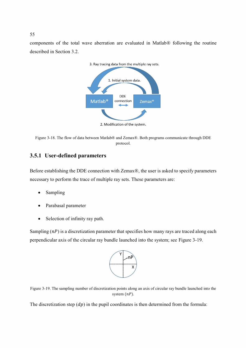
55
components of the total wave aberration are evaluated in Matlab® following the routine
described in Section 3.2.
Figure 3-18. The flow of data between Matlab® and Zemax®. Both programs communicate through DDE
protocol.
3.5.1 User-defined parameters
Before establishing the DDE connection with Zemax®, the user is asked to specify parameters
necessary to perform the trace of multiple ray sets. These parameters are:
• Sampling
• Parabasal parameter
• Selection of infinity ray path.
Sampling (𝑛𝑃) is a discretization parameter that specifies how many rays are traced along each
perpendicular axis of the circular ray bundle launched into the system; see Figure 3-19.
Figure 3-19. The sampling number of discretization points along an axis of circular ray bundle launched into the
system (𝑛𝑃).
The discretization step (𝑑𝑝) in the pupil coordinates is then determined from the formula:
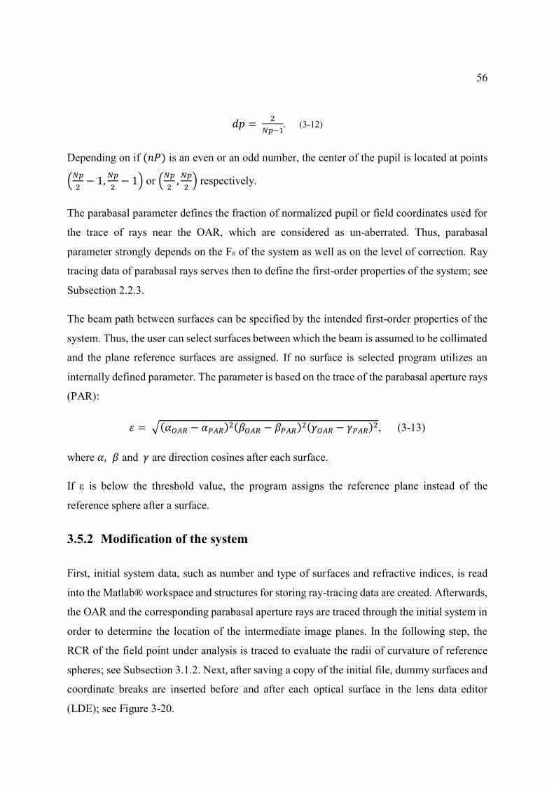
56
𝑑𝑝 = 2
𝑁𝑝−1. (3-12)
Depending on if (𝑛𝑃) is an even or an odd number, the center of the pupil is located at points
(𝑁𝑝
2− 1,
𝑁𝑝
2− 1) or (
𝑁𝑝
2,𝑁𝑝
2) respectively.
The parabasal parameter defines the fraction of normalized pupil or field coordinates used for
the trace of rays near the OAR, which are considered as un-aberrated. Thus, parabasal
parameter strongly depends on the F# of the system as well as on the level of correction. Ray
tracing data of parabasal rays serves then to define the first-order properties of the system; see
Subsection 2.2.3.
The beam path between surfaces can be specified by the intended first-order properties of the
system. Thus, the user can select surfaces between which the beam is assumed to be collimated
and the plane reference surfaces are assigned. If no surface is selected program utilizes an
internally defined parameter. The parameter is based on the trace of the parabasal aperture rays
(PAR):
𝜀 = √(𝛼𝑂𝐴𝑅 − 𝛼𝑃𝐴𝑅)2(𝛽𝑂𝐴𝑅 − 𝛽𝑃𝐴𝑅)2(𝛾𝑂𝐴𝑅 − 𝛾𝑃𝐴𝑅)2, (3-13)
where 𝛼, 𝛽 and 𝛾 are direction cosines after each surface.
If ε is below the threshold value, the program assigns the reference plane instead of the
reference sphere after a surface.
3.5.2 Modification of the system
First, initial system data, such as number and type of surfaces and refractive indices, is read
into the Matlab® workspace and structures for storing ray-tracing data are created. Afterwards,
the OAR and the corresponding parabasal aperture rays are traced through the initial system in
order to determine the location of the intermediate image planes. In the following step, the
RCR of the field point under analysis is traced to evaluate the radii of curvature of reference
spheres; see Subsection 3.1.2. Next, after saving a copy of the initial file, dummy surfaces and
coordinate breaks are inserted before and after each optical surface in the lens data editor
(LDE); see Figure 3-20.
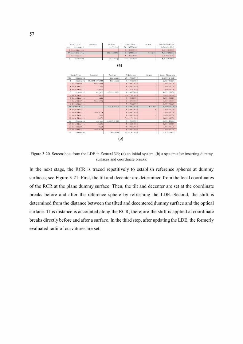
57
Figure 3-20. Screenshots from the LDE in Zemax13®; (a) an initial system, (b) a system after inserting dummy
surfaces and coordinate breaks.
In the next stage, the RCR is traced repetitively to establish reference spheres at dummy
surfaces; see Figure 3-21. First, the tilt and decenter are determined from the local coordinates
of the RCR at the plane dummy surface. Then, the tilt and decenter are set at the coordinate
breaks before and after the reference sphere by refreshing the LDE. Second, the shift is
determined from the distance between the tilted and decentered dummy surface and the optical
surface. This distance is accounted along the RCR, therefore the shift is applied at coordinate
breaks directly before and after a surface. In the third step, after updating the LDE, the formerly
evaluated radii of curvatures are set.
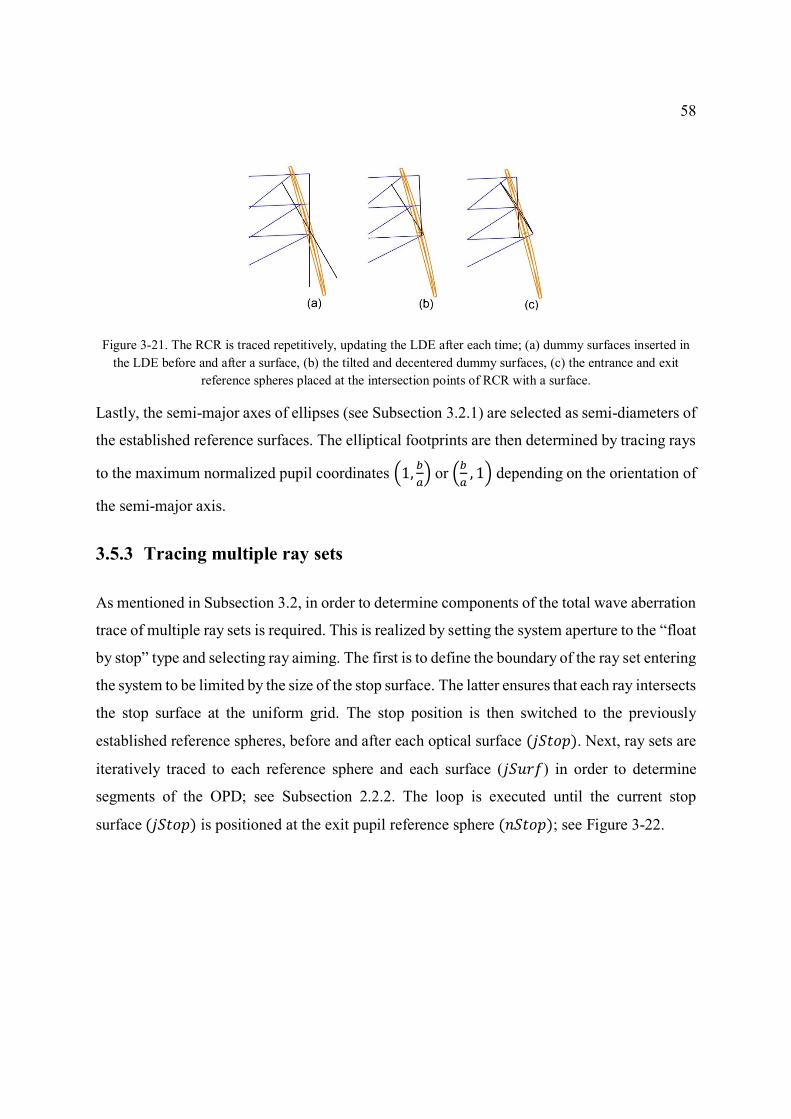
58
Figure 3-21. The RCR is traced repetitively, updating the LDE after each time; (a) dummy surfaces inserted in
the LDE before and after a surface, (b) the tilted and decentered dummy surfaces, (c) the entrance and exit
reference spheres placed at the intersection points of RCR with a surface.
Lastly, the semi-major axes of ellipses (see Subsection 3.2.1) are selected as semi-diameters of
the established reference surfaces. The elliptical footprints are then determined by tracing rays
to the maximum normalized pupil coordinates (1,𝑏
𝑎) or (
𝑏
𝑎, 1) depending on the orientation of
the semi-major axis.
3.5.3 Tracing multiple ray sets
As mentioned in Subsection 3.2, in order to determine components of the total wave aberration
trace of multiple ray sets is required. This is realized by setting the system aperture to the “float
by stop” type and selecting ray aiming. The first is to define the boundary of the ray set entering
the system to be limited by the size of the stop surface. The latter ensures that each ray intersects
the stop surface at the uniform grid. The stop position is then switched to the previously
established reference spheres, before and after each optical surface (𝑗𝑆𝑡𝑜𝑝). Next, ray sets are
iteratively traced to each reference sphere and each surface (𝑗𝑆𝑢𝑟𝑓) in order to determine
segments of the OPD; see Subsection 2.2.2. The loop is executed until the current stop
surface (𝑗𝑆𝑡𝑜𝑝) is positioned at the exit pupil reference sphere (𝑛𝑆𝑡𝑜𝑝); see Figure 3-22.
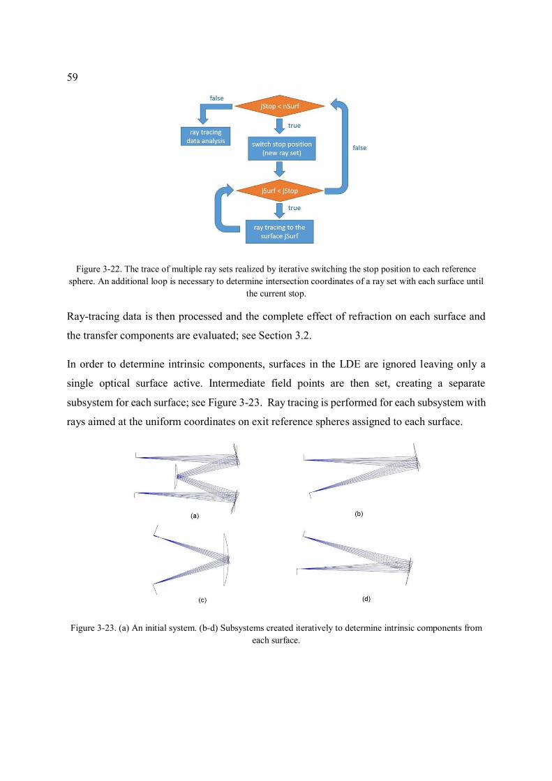
59
Figure 3-22. The trace of multiple ray sets realized by iterative switching the stop position to each reference
sphere. An additional loop is necessary to determine intersection coordinates of a ray set with each surface until
the current stop.
Ray-tracing data is then processed and the complete effect of refraction on each surface and
the transfer components are evaluated; see Section 3.2.
In order to determine intrinsic components, surfaces in the LDE are ignored leaving only a
single optical surface active. Intermediate field points are then set, creating a separate
subsystem for each surface; see Figure 3-23. Ray tracing is performed for each subsystem with
rays aimed at the uniform coordinates on exit reference spheres assigned to each surface.
Figure 3-23. (a) An initial system. (b-d) Subsystems created iteratively to determine intrinsic components from
each surface.
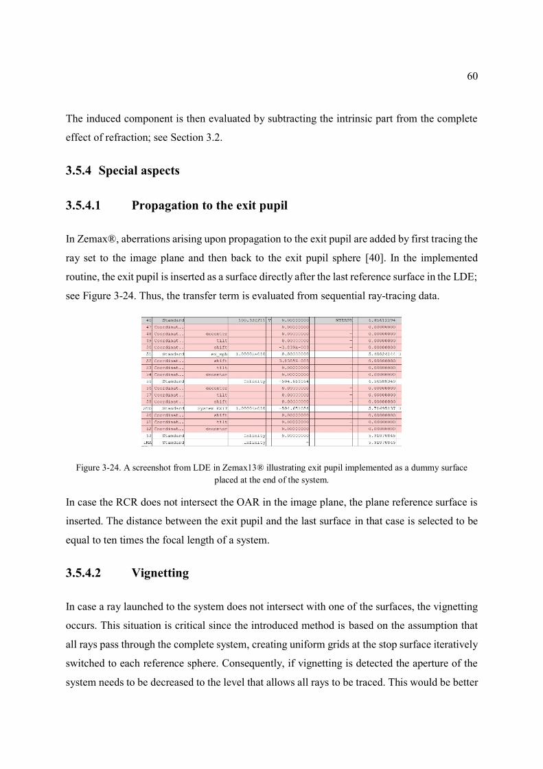
60
The induced component is then evaluated by subtracting the intrinsic part from the complete
effect of refraction; see Section 3.2.
3.5.4 Special aspects
3.5.4.1 Propagation to the exit pupil
In Zemax®, aberrations arising upon propagation to the exit pupil are added by first tracing the
ray set to the image plane and then back to the exit pupil sphere [40]. In the implemented
routine, the exit pupil is inserted as a surface directly after the last reference surface in the LDE;
see Figure 3-24. Thus, the transfer term is evaluated from sequential ray-tracing data.
Figure 3-24. A screenshot from LDE in Zemax13® illustrating exit pupil implemented as a dummy surface
placed at the end of the system.
In case the RCR does not intersect the OAR in the image plane, the plane reference surface is
inserted. The distance between the exit pupil and the last surface in that case is selected to be
equal to ten times the focal length of a system.
3.5.4.2 Vignetting
In case a ray launched to the system does not intersect with one of the surfaces, the vignetting
occurs. This situation is critical since the introduced method is based on the assumption that
all rays pass through the complete system, creating uniform grids at the stop surface iteratively
switched to each reference sphere. Consequently, if vignetting is detected the aperture of the
system needs to be decreased to the level that allows all rays to be traced. This would be better
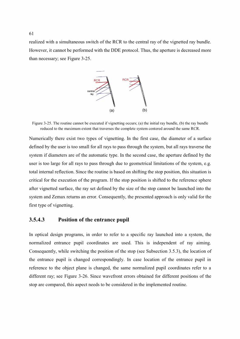
61
realized with a simultaneous switch of the RCR to the central ray of the vignetted ray bundle.
However, it cannot be performed with the DDE protocol. Thus, the aperture is decreased more
than necessary; see Figure 3-25.
Figure 3-25. The routine cannot be executed if vignetting occurs; (a) the initial ray bundle, (b) the ray bundle
reduced to the maximum extent that traverses the complete system centered around the same RCR.
Numerically there exist two types of vignetting. In the first case, the diameter of a surface
defined by the user is too small for all rays to pass through the system, but all rays traverse the
system if diameters are of the automatic type. In the second case, the aperture defined by the
user is too large for all rays to pass through due to geometrical limitations of the system, e.g.
total internal reflection. Since the routine is based on shifting the stop position, this situation is
critical for the execution of the program. If the stop position is shifted to the reference sphere
after vignetted surface, the ray set defined by the size of the stop cannot be launched into the
system and Zemax returns an error. Consequently, the presented approach is only valid for the
first type of vignetting.
3.5.4.3 Position of the entrance pupil
In optical design programs, in order to refer to a specific ray launched into a system, the
normalized entrance pupil coordinates are used. This is independent of ray aiming.
Consequently, while switching the position of the stop (see Subsection 3.5.3), the location of
the entrance pupil is changed correspondingly. In case location of the entrance pupil in
reference to the object plane is changed, the same normalized pupil coordinates refer to a
different ray; see Figure 3-26. Since wavefront errors obtained for different positions of the
stop are compared, this aspect needs to be considered in the implemented routine.
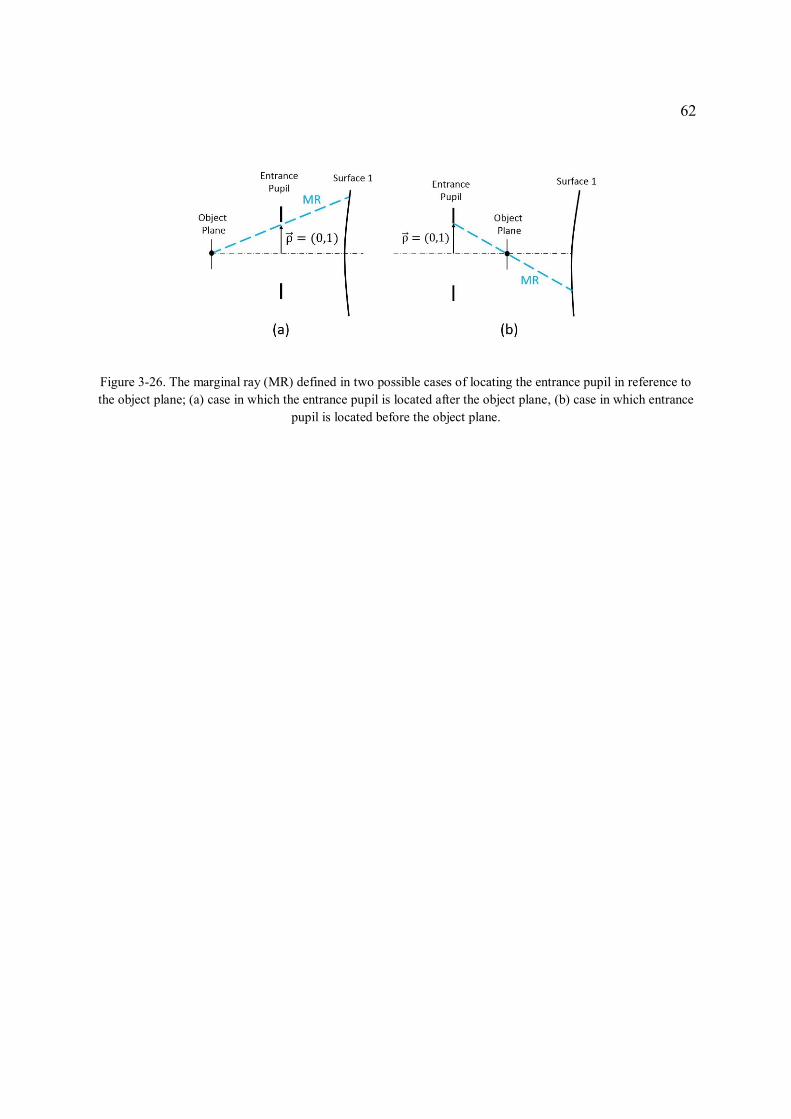
62
Figure 3-26. The marginal ray (MR) defined in two possible cases of locating the entrance pupil in reference to
the object plane; (a) case in which the entrance pupil is located after the object plane, (b) case in which entrance
pupil is located before the object plane.
63
Chapter 4 Application
In the design process of a freeform system, it is important to utilize additional design variables
in the most effective way [21]. The simple approach of adding freeform sag contribution to one
or more elements in the system may result in an “over-engineered” solution with an
unnecessarily large deviation of sag from the basic shape; see Section 2.4. Thus, analysis of
aberrations generated in the system utilizing the same description (Zernike fringe set) as the
one used for the freeform sag, is a valuable tool in designing freeform systems. In the following
chapter, it is presented how analysis of the Zernike surface contributions can assist in selecting
the most effective first-order configuration and a position of the freeform element in the system.
4.1 Relations between low- and higher-order Zernike
aberrations
Imaging performance of freeform mirror systems in the final design stage is typically limited
by higher-order Zernike aberrations. Thus, the knowledge of how higher-order aberrations are
generated is of crucial importance in the design process of such systems. As known from
aberration theory of axially symmetric systems, the higher-order aberration coefficients depend
on primary aberrations and the first-order ray properties; see Subsection 2.1.5. General
dependencies that occur in formulas for the sixth-order intrinsic wave aberration coefficients
(see Table 2-3) can provide valuable insights for the interpretation of numerically obtained
Zernike terms. Thus, taking into account these relations, following dependencies are
formulated for the intrinsic Zernike aberration components of a single field point:
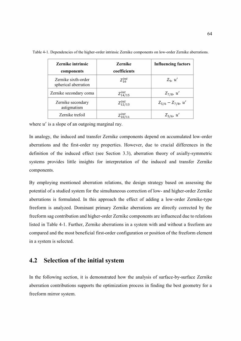
64
Table 4-1. Dependencies of the higher-order intrinsic Zernike components on low-order Zernike aberrations.
Zernike intrinsic
components
Zernike
coefficients
Influencing factors
Zernike sixth-order
spherical aberration 𝑍16
𝑖𝑛𝑡 𝑍9, 𝑢′
Zernike secondary coma 𝑍14/15𝑖𝑛𝑡 𝑍7/8, 𝑢
′
Zernike secondary
astigmatism 𝑍12/13
𝑖𝑛𝑡 𝑍5/6 − 𝑍7/8, 𝑢′
Zernike trefoil 𝑍10/11𝑖𝑛𝑡 𝑍5/6, 𝑢
′
where 𝑢′ is a slope of an outgoing marginal ray.
In analogy, the induced and transfer Zernike components depend on accumulated low-order
aberrations and the first-order ray properties. However, due to crucial differences in the
definition of the induced effect (see Section 3.3), aberration theory of axially-symmetric
systems provides little insights for interpretation of the induced and transfer Zernike
components.
By employing mentioned aberration relations, the design strategy based on assessing the
potential of a studied system for the simultaneous correction of low- and higher-order Zernike
aberrations is formulated. In this approach the effect of adding a low-order Zernike-type
freeform is analyzed. Dominant primary Zernike aberrations are directly corrected by the
freeform sag contribution and higher-order Zernike components are influenced due to relations
listed in Table 4-1. Further, Zernike aberrations in a system with and without a freeform are
compared and the most beneficial first-order configuration or position of the freeform element
in a system is selected.
4.2 Selection of the initial system
In the following section, it is demonstrated how the analysis of surface-by-surface Zernike
aberration contributions supports the optimization process in finding the best geometry for a
freeform mirror system.
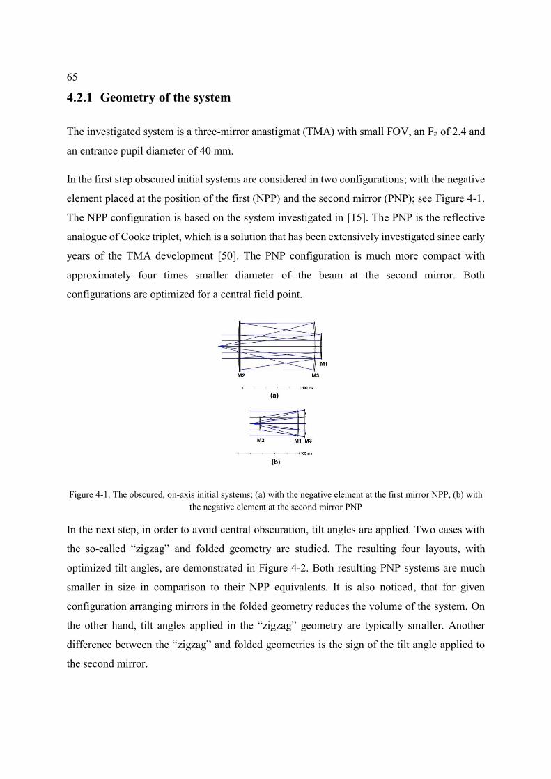
65
4.2.1 Geometry of the system
The investigated system is a three-mirror anastigmat (TMA) with small FOV, an F# of 2.4 and
an entrance pupil diameter of 40 mm.
In the first step obscured initial systems are considered in two configurations; with the negative
element placed at the position of the first (NPP) and the second mirror (PNP); see Figure 4-1.
The NPP configuration is based on the system investigated in [15]. The PNP is the reflective
analogue of Cooke triplet, which is a solution that has been extensively investigated since early
years of the TMA development [50]. The PNP configuration is much more compact with
approximately four times smaller diameter of the beam at the second mirror. Both
configurations are optimized for a central field point.
Figure 4-1. The obscured, on-axis initial systems; (a) with the negative element at the first mirror NPP, (b) with
the negative element at the second mirror PNP
In the next step, in order to avoid central obscuration, tilt angles are applied. Two cases with
the so-called “zigzag” and folded geometry are studied. The resulting four layouts, with
optimized tilt angles, are demonstrated in Figure 4-2. Both resulting PNP systems are much
smaller in size in comparison to their NPP equivalents. It is also noticed, that for given
configuration arranging mirrors in the folded geometry reduces the volume of the system. On
the other hand, tilt angles applied in the “zigzag” geometry are typically smaller. Another
difference between the “zigzag” and folded geometries is the sign of the tilt angle applied to
the second mirror.
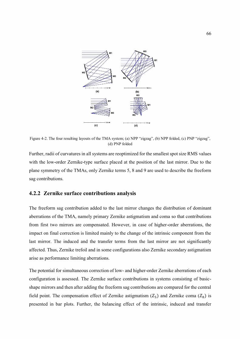
66
Figure 4-2. The four resulting layouts of the TMA system; (a) NPP “zigzag”, (b) NPP folded, (c) PNP “zigzag”,
(d) PNP folded
Further, radii of curvatures in all systems are reoptimized for the smallest spot size RMS values
with the low-order Zernike-type surface placed at the position of the last mirror. Due to the
plane symmetry of the TMAs, only Zernike terms 5, 8 and 9 are used to describe the freeform
sag contributions.
4.2.2 Zernike surface contributions analysis
The freeform sag contribution added to the last mirror changes the distribution of dominant
aberrations of the TMA, namely primary Zernike astigmatism and coma so that contributions
from first two mirrors are compensated. However, in case of higher-order aberrations, the
impact on final correction is limited mainly to the change of the intrinsic component from the
last mirror. The induced and the transfer terms from the last mirror are not significantly
affected. Thus, Zernike trefoil and in some configurations also Zernike secondary astigmatism
arise as performance limiting aberrations.
The potential for simultaneous correction of low- and higher-order Zernike aberrations of each
configuration is assessed. The Zernike surface contributions in systems consisting of basic-
shape mirrors and then after adding the freeform sag contributions are compared for the central
field point. The compensation effect of Zernike astigmatism (𝑍5) and Zernike coma (𝑍8) is
presented in bar plots. Further, the balancing effect of the intrinsic, induced and transfer
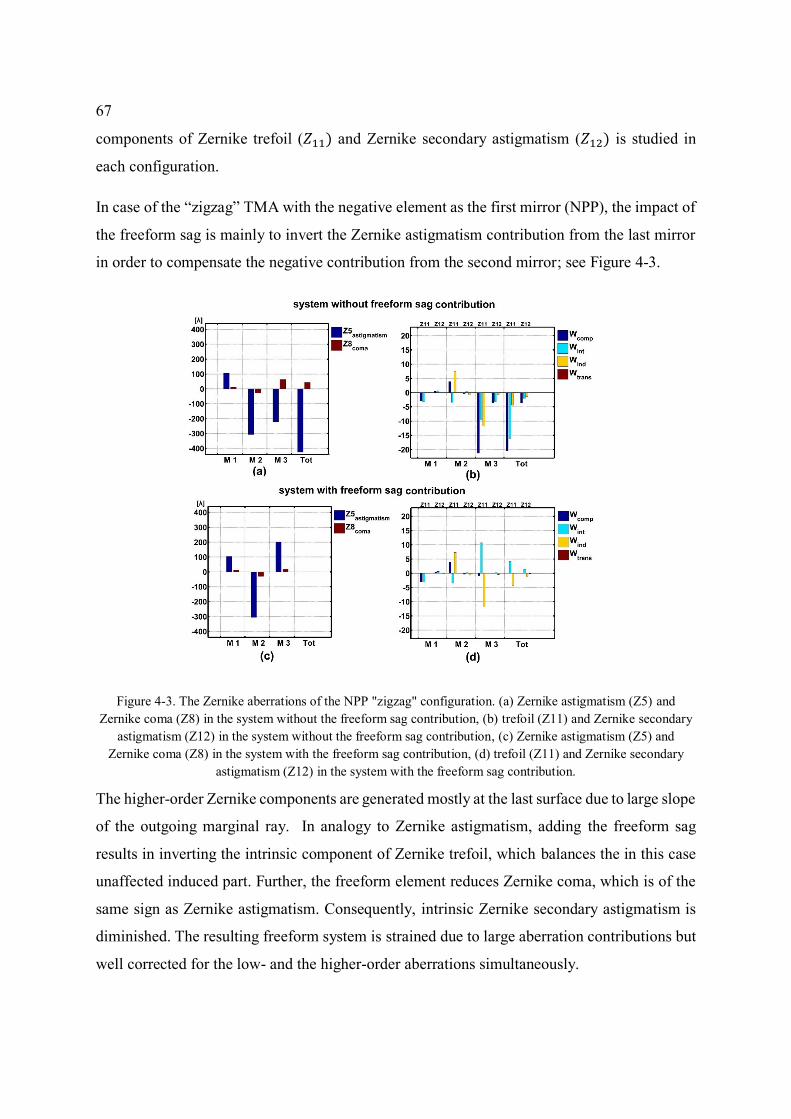
67
components of Zernike trefoil (𝑍11) and Zernike secondary astigmatism (𝑍12) is studied in
each configuration.
In case of the “zigzag” TMA with the negative element as the first mirror (NPP), the impact of
the freeform sag is mainly to invert the Zernike astigmatism contribution from the last mirror
in order to compensate the negative contribution from the second mirror; see Figure 4-3.
Figure 4-3. The Zernike aberrations of the NPP "zigzag" configuration. (a) Zernike astigmatism (Z5) and
Zernike coma (Z8) in the system without the freeform sag contribution, (b) trefoil (Z11) and Zernike secondary
astigmatism (Z12) in the system without the freeform sag contribution, (c) Zernike astigmatism (Z5) and
Zernike coma (Z8) in the system with the freeform sag contribution, (d) trefoil (Z11) and Zernike secondary
astigmatism (Z12) in the system with the freeform sag contribution.
The higher-order Zernike components are generated mostly at the last surface due to large slope
of the outgoing marginal ray. In analogy to Zernike astigmatism, adding the freeform sag
results in inverting the intrinsic component of Zernike trefoil, which balances the in this case
unaffected induced part. Further, the freeform element reduces Zernike coma, which is of the
same sign as Zernike astigmatism. Consequently, intrinsic Zernike secondary astigmatism is
diminished. The resulting freeform system is strained due to large aberration contributions but
well corrected for the low- and the higher-order aberrations simultaneously.
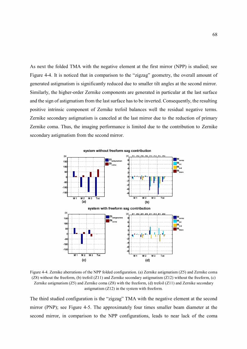
68
As next the folded TMA with the negative element at the first mirror (NPP) is studied; see
Figure 4-4. It is noticed that in comparison to the “zigzag” geometry, the overall amount of
generated astigmatism is significantly reduced due to smaller tilt angles at the second mirror.
Similarly, the higher-order Zernike components are generated in particular at the last surface
and the sign of astigmatism from the last surface has to be inverted. Consequently, the resulting
positive intrinsic component of Zernike trefoil balances well the residual negative terms.
Zernike secondary astigmatism is canceled at the last mirror due to the reduction of primary
Zernike coma. Thus, the imaging performance is limited due to the contribution to Zernike
secondary astigmatism from the second mirror.
Figure 4-4. Zernike aberrations of the NPP folded configuration. (a) Zernike astigmatism (Z5) and Zernike coma
(Z8) without the freeform, (b) trefoil (Z11) and Zernike secondary astigmatism (Z12) without the freeform, (c)
Zernike astigmatism (Z5) and Zernike coma (Z8) with the freeform, (d) trefoil (Z11) and Zernike secondary
astigmatism (Z12) in the system with freeform.
The third studied configuration is the “zigzag” TMA with the negative element at the second
mirror (PNP); see Figure 4-5. The approximately four times smaller beam diameter at the
second mirror, in comparison to the NPP configurations, leads to near lack of the coma
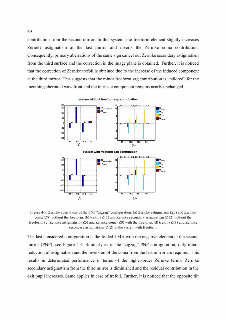
69
contribution from the second mirror. In this system, the freeform element slightly increases
Zernike astigmatism at the last mirror and inverts the Zernike coma contribution.
Consequently, primary aberrations of the same sign cancel out Zernike secondary astigmatism
from the third surface and the correction in the image plane is obtained. Further, it is noticed
that the correction of Zernike trefoil is obtained due to the increase of the induced component
at the third mirror. This suggests that the minor freeform sag contribution is “tailored” for the
incoming aberrated wavefront and the intrinsic component remains nearly unchanged.
Figure 4-5. Zernike aberrations of the PNP “zigzag” configuration. (a) Zernike astigmatism (Z5) and Zernike
coma (Z8) without the freeform, (b) trefoil (Z11) and Zernike secondary astigmatism (Z12) without the
freeform, (c) Zernike astigmatism (Z5) and Zernike coma (Z8) with the freeform, (d) trefoil (Z11) and Zernike
secondary astigmatism (Z12) in the system with freeform.
The last considered configuration is the folded TMA with the negative element at the second
mirror (PNP); see Figure 4-6. Similarly as in the “zigzag” PNP configuration, only minor
reduction of astigmatism and the inversion of the coma from the last mirror are required. This
results in deteriorated performance in terms of the higher-order Zernike terms. Zernike
secondary astigmatism from the third mirror is diminished and the residual contribution in the
exit pupil increases. Same applies in case of trefoil. Further, it is noticed that the opposite tilt
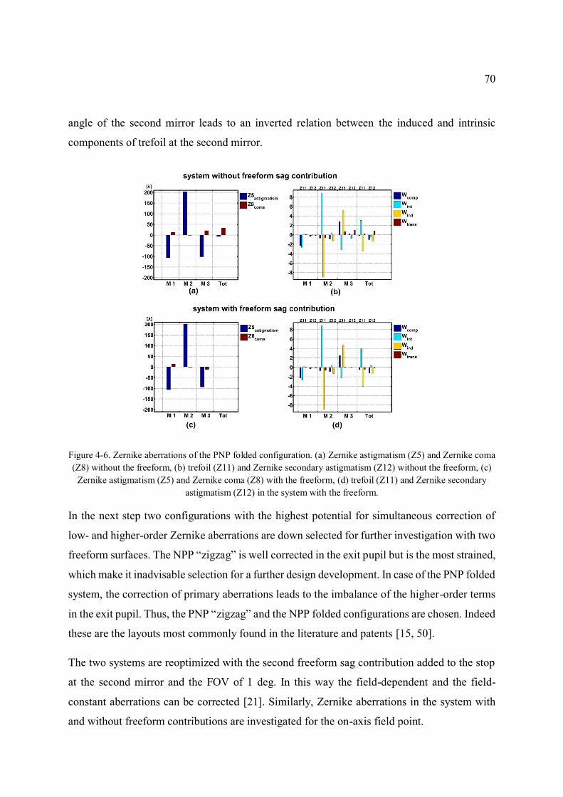
70
angle of the second mirror leads to an inverted relation between the induced and intrinsic
components of trefoil at the second mirror.
Figure 4-6. Zernike aberrations of the PNP folded configuration. (a) Zernike astigmatism (Z5) and Zernike coma
(Z8) without the freeform, (b) trefoil (Z11) and Zernike secondary astigmatism (Z12) without the freeform, (c)
Zernike astigmatism (Z5) and Zernike coma (Z8) with the freeform, (d) trefoil (Z11) and Zernike secondary
astigmatism (Z12) in the system with the freeform.
In the next step two configurations with the highest potential for simultaneous correction of
low- and higher-order Zernike aberrations are down selected for further investigation with two
freeform surfaces. The NPP “zigzag” is well corrected in the exit pupil but is the most strained,
which make it inadvisable selection for a further design development. In case of the PNP folded
system, the correction of primary aberrations leads to the imbalance of the higher-order terms
in the exit pupil. Thus, the PNP “zigzag” and the NPP folded configurations are chosen. Indeed
these are the layouts most commonly found in the literature and patents [15, 50].
The two systems are reoptimized with the second freeform sag contribution added to the stop
at the second mirror and the FOV of 1 deg. In this way the field-dependent and the field-
constant aberrations can be corrected [21]. Similarly, Zernike aberrations in the system with
and without freeform contributions are investigated for the on-axis field point.
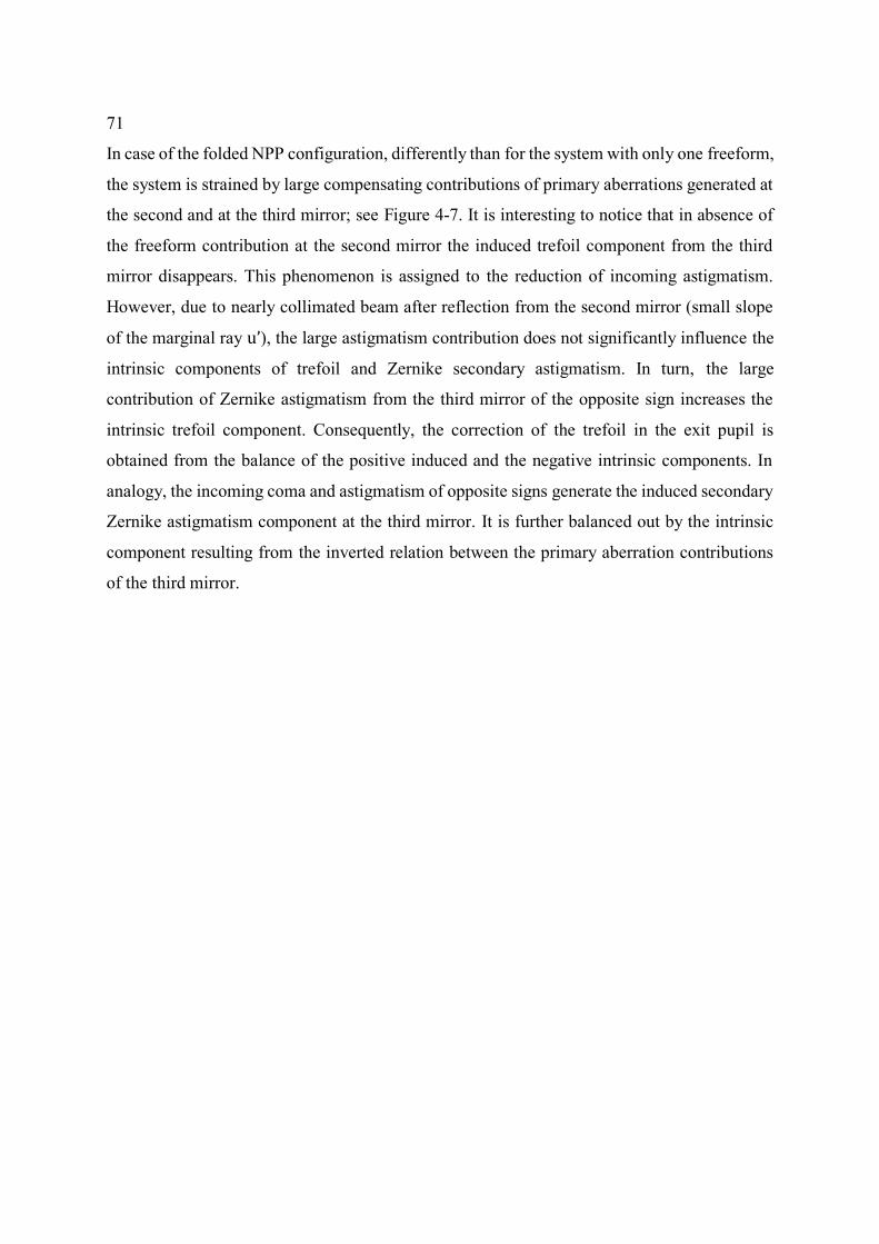
71
In case of the folded NPP configuration, differently than for the system with only one freeform,
the system is strained by large compensating contributions of primary aberrations generated at
the second and at the third mirror; see Figure 4-7. It is interesting to notice that in absence of
the freeform contribution at the second mirror the induced trefoil component from the third
mirror disappears. This phenomenon is assigned to the reduction of incoming astigmatism.
However, due to nearly collimated beam after reflection from the second mirror (small slope
of the marginal ray u’), the large astigmatism contribution does not significantly influence the
intrinsic components of trefoil and Zernike secondary astigmatism. In turn, the large
contribution of Zernike astigmatism from the third mirror of the opposite sign increases the
intrinsic trefoil component. Consequently, the correction of the trefoil in the exit pupil is
obtained from the balance of the positive induced and the negative intrinsic components. In
analogy, the incoming coma and astigmatism of opposite signs generate the induced secondary
Zernike astigmatism component at the third mirror. It is further balanced out by the intrinsic
component resulting from the inverted relation between the primary aberration contributions
of the third mirror.
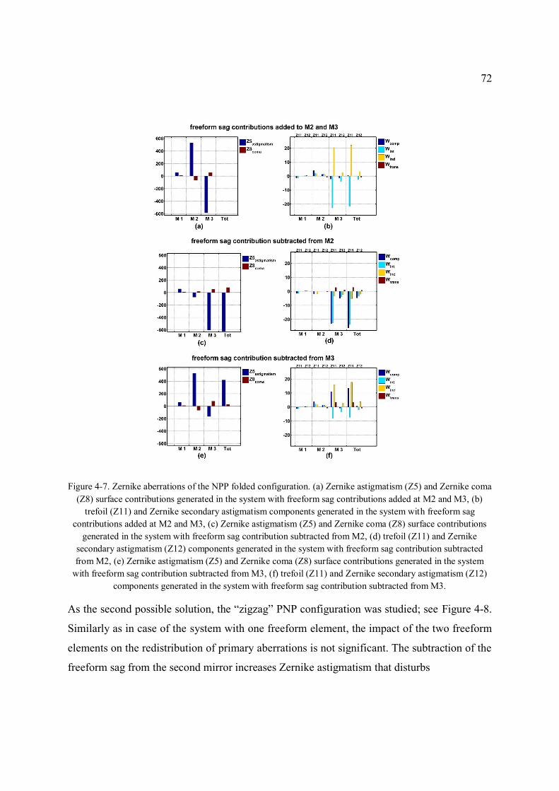
72
Figure 4-7. Zernike aberrations of the NPP folded configuration. (a) Zernike astigmatism (Z5) and Zernike coma
(Z8) surface contributions generated in the system with freeform sag contributions added at M2 and M3, (b)
trefoil (Z11) and Zernike secondary astigmatism components generated in the system with freeform sag
contributions added at M2 and M3, (c) Zernike astigmatism (Z5) and Zernike coma (Z8) surface contributions
generated in the system with freeform sag contribution subtracted from M2, (d) trefoil (Z11) and Zernike
secondary astigmatism (Z12) components generated in the system with freeform sag contribution subtracted
from M2, (e) Zernike astigmatism (Z5) and Zernike coma (Z8) surface contributions generated in the system
with freeform sag contribution subtracted from M3, (f) trefoil (Z11) and Zernike secondary astigmatism (Z12)
components generated in the system with freeform sag contribution subtracted from M3.
As the second possible solution, the “zigzag” PNP configuration was studied; see Figure 4-8.
Similarly as in case of the system with one freeform element, the impact of the two freeform
elements on the redistribution of primary aberrations is not significant. The subtraction of the
freeform sag from the second mirror increases Zernike astigmatism that disturbs
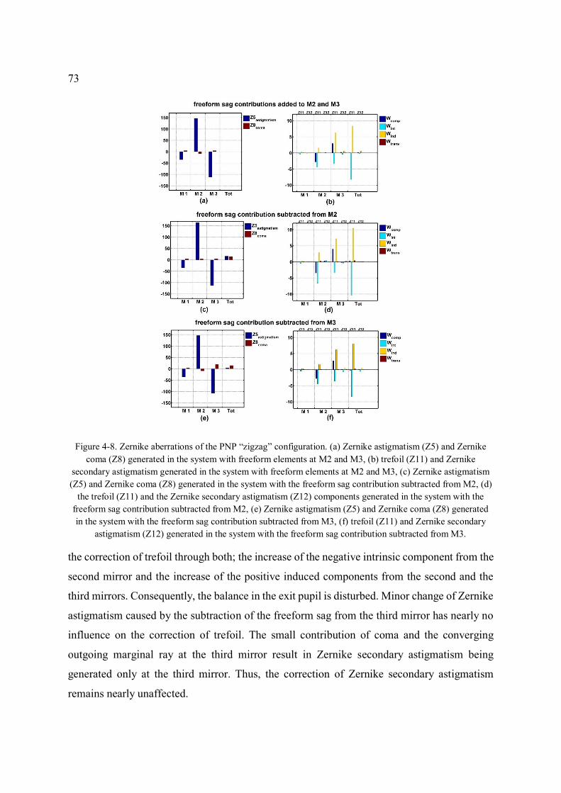
73
Figure 4-8. Zernike aberrations of the PNP “zigzag” configuration. (a) Zernike astigmatism (Z5) and Zernike
coma (Z8) generated in the system with freeform elements at M2 and M3, (b) trefoil (Z11) and Zernike
secondary astigmatism generated in the system with freeform elements at M2 and M3, (c) Zernike astigmatism
(Z5) and Zernike coma (Z8) generated in the system with the freeform sag contribution subtracted from M2, (d)
the trefoil (Z11) and the Zernike secondary astigmatism (Z12) components generated in the system with the
freeform sag contribution subtracted from M2, (e) Zernike astigmatism (Z5) and Zernike coma (Z8) generated
in the system with the freeform sag contribution subtracted from M3, (f) trefoil (Z11) and Zernike secondary
astigmatism (Z12) generated in the system with the freeform sag contribution subtracted from M3.
the correction of trefoil through both; the increase of the negative intrinsic component from the
second mirror and the increase of the positive induced components from the second and the
third mirrors. Consequently, the balance in the exit pupil is disturbed. Minor change of Zernike
astigmatism caused by the subtraction of the freeform sag from the third mirror has nearly no
influence on the correction of trefoil. The small contribution of coma and the converging
outgoing marginal ray at the third mirror result in Zernike secondary astigmatism being
generated only at the third mirror. Thus, the correction of Zernike secondary astigmatism
remains nearly unaffected.
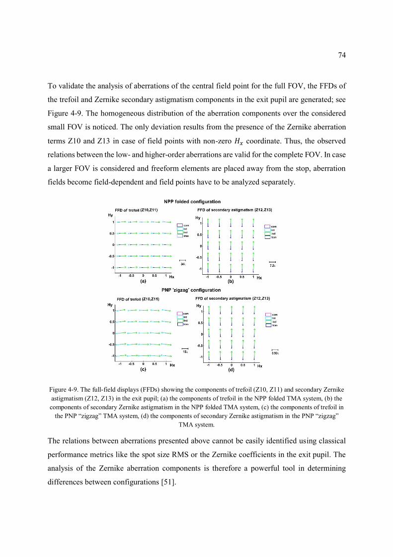
74
To validate the analysis of aberrations of the central field point for the full FOV, the FFDs of
the trefoil and Zernike secondary astigmatism components in the exit pupil are generated; see
Figure 4-9. The homogeneous distribution of the aberration components over the considered
small FOV is noticed. The only deviation results from the presence of the Zernike aberration
terms Z10 and Z13 in case of field points with non-zero 𝐻𝑥 coordinate. Thus, the observed
relations between the low- and higher-order aberrations are valid for the complete FOV. In case
a larger FOV is considered and freeform elements are placed away from the stop, aberration
fields become field-dependent and field points have to be analyzed separately.
Figure 4-9. The full-field displays (FFDs) showing the components of trefoil (Z10, Z11) and secondary Zernike
astigmatism (Z12, Z13) in the exit pupil; (a) the components of trefoil in the NPP folded TMA system, (b) the
components of secondary Zernike astigmatism in the NPP folded TMA system, (c) the components of trefoil in
the PNP “zigzag” TMA system, (d) the components of secondary Zernike astigmatism in the PNP “zigzag”
TMA system.
The relations between aberrations presented above cannot be easily identified using classical
performance metrics like the spot size RMS or the Zernike coefficients in the exit pupil. The
analysis of the Zernike aberration components is therefore a powerful tool in determining
differences between configurations [51].
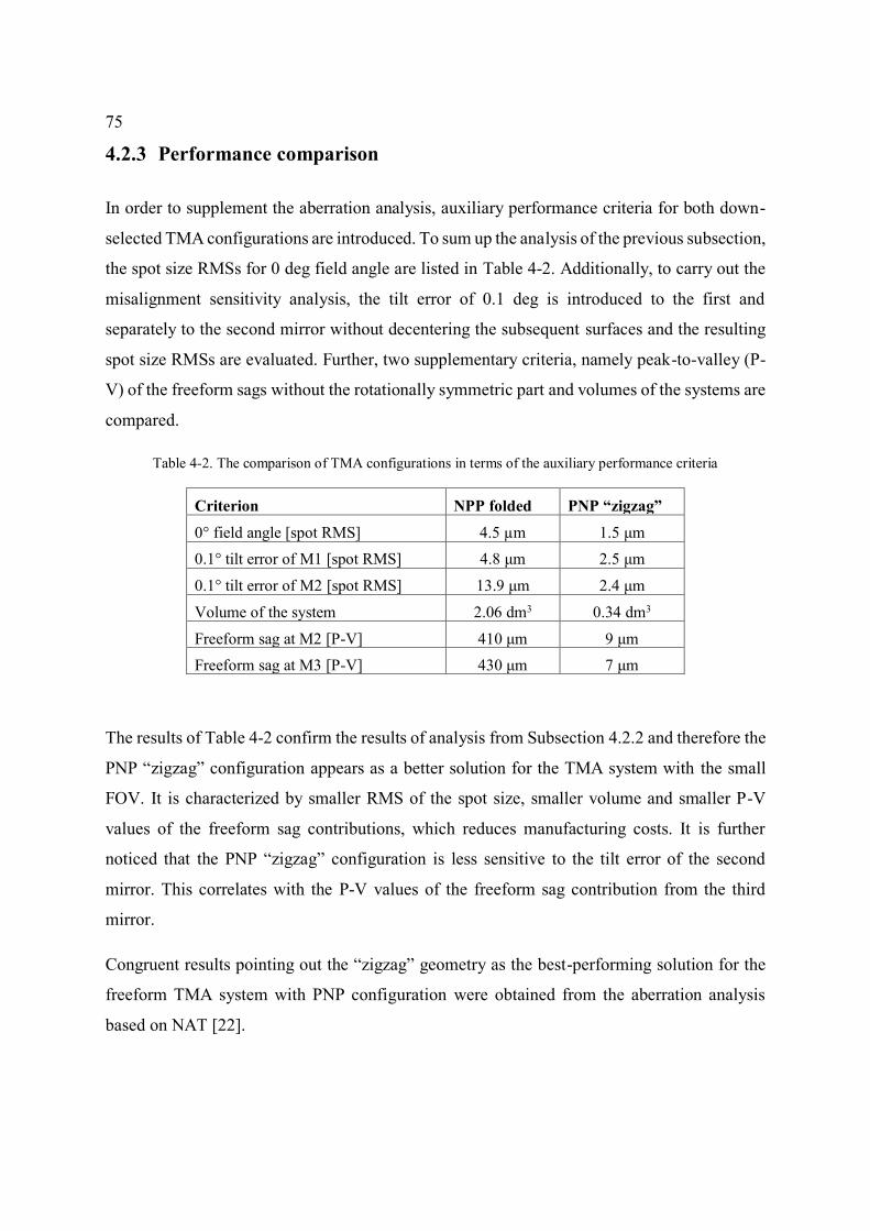
75
4.2.3 Performance comparison
In order to supplement the aberration analysis, auxiliary performance criteria for both down-
selected TMA configurations are introduced. To sum up the analysis of the previous subsection,
the spot size RMSs for 0 deg field angle are listed in Table 4-2. Additionally, to carry out the
misalignment sensitivity analysis, the tilt error of 0.1 deg is introduced to the first and
separately to the second mirror without decentering the subsequent surfaces and the resulting
spot size RMSs are evaluated. Further, two supplementary criteria, namely peak-to-valley (P-
V) of the freeform sags without the rotationally symmetric part and volumes of the systems are
compared.
Table 4-2. The comparison of TMA configurations in terms of the auxiliary performance criteria
Criterion NPP folded PNP “zigzag”
0° field angle [spot RMS] 4.5 µm 1.5 μm
0.1° tilt error of M1 [spot RMS] 4.8 μm 2.5 μm
0.1° tilt error of M2 [spot RMS] 13.9 μm 2.4 μm
Volume of the system 2.06 dm3 0.34 dm3
Freeform sag at M2 [P-V] 410 μm 9 μm
Freeform sag at M3 [P-V] 430 μm 7 μm
The results of Table 4-2 confirm the results of analysis from Subsection 4.2.2 and therefore the
PNP “zigzag” configuration appears as a better solution for the TMA system with the small
FOV. It is characterized by smaller RMS of the spot size, smaller volume and smaller P-V
values of the freeform sag contributions, which reduces manufacturing costs. It is further
noticed that the PNP “zigzag” configuration is less sensitive to the tilt error of the second
mirror. This correlates with the P-V values of the freeform sag contribution from the third
mirror.
Congruent results pointing out the “zigzag” geometry as the best-performing solution for the
freeform TMA system with PNP configuration were obtained from the aberration analysis
based on NAT [22].
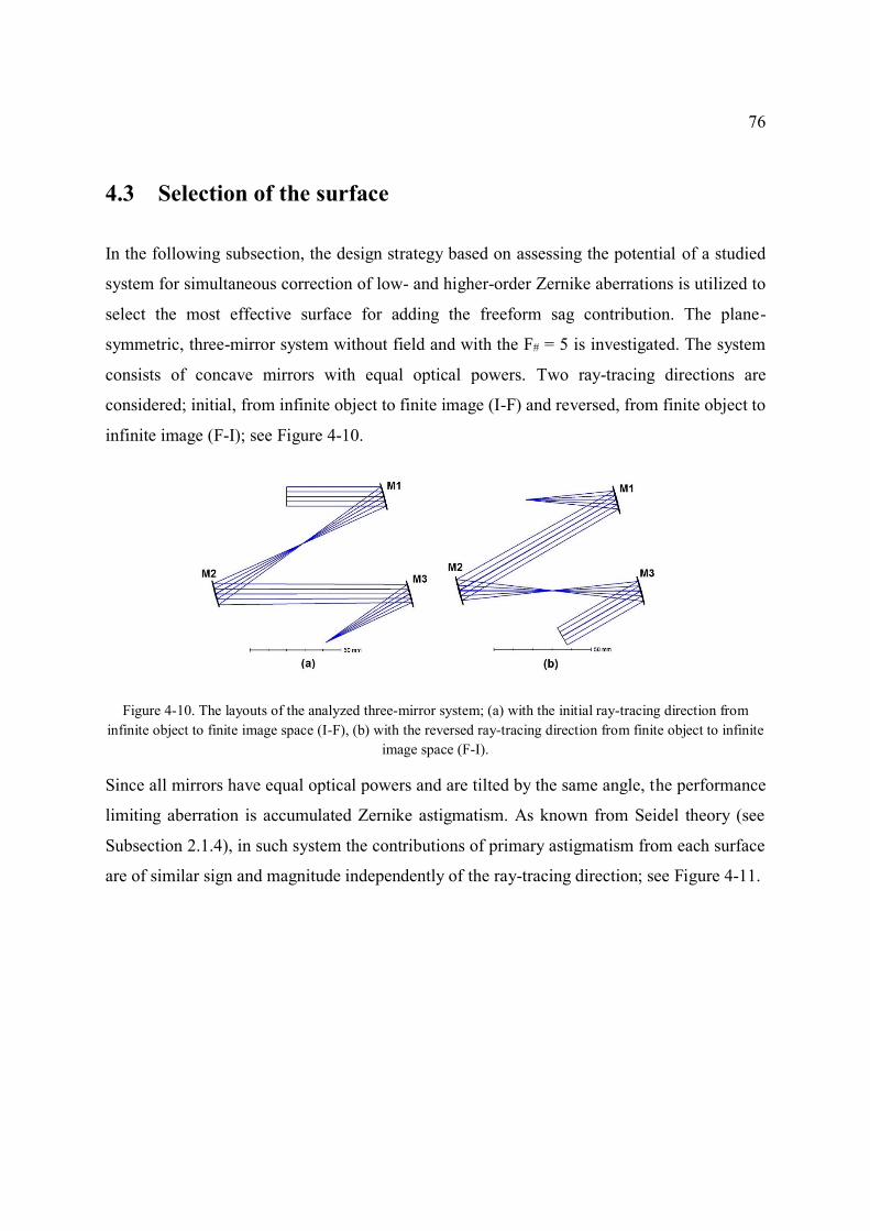
76
4.3 Selection of the surface
In the following subsection, the design strategy based on assessing the potential of a studied
system for simultaneous correction of low- and higher-order Zernike aberrations is utilized to
select the most effective surface for adding the freeform sag contribution. The plane-
symmetric, three-mirror system without field and with the F# = 5 is investigated. The system
consists of concave mirrors with equal optical powers. Two ray-tracing directions are
considered; initial, from infinite object to finite image (I-F) and reversed, from finite object to
infinite image (F-I); see Figure 4-10.
Figure 4-10. The layouts of the analyzed three-mirror system; (a) with the initial ray-tracing direction from
infinite object to finite image space (I-F), (b) with the reversed ray-tracing direction from finite object to infinite
image space (F-I).
Since all mirrors have equal optical powers and are tilted by the same angle, the performance
limiting aberration is accumulated Zernike astigmatism. As known from Seidel theory (see
Subsection 2.1.4), in such system the contributions of primary astigmatism from each surface
are of similar sign and magnitude independently of the ray-tracing direction; see Figure 4-11.
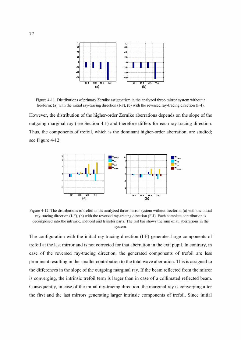
77
Figure 4-11. Distributions of primary Zernike astigmatism in the analyzed three-mirror system without a
freeform; (a) with the initial ray-tracing direction (I-F), (b) with the reversed ray-tracing direction (F-I).
However, the distribution of the higher-order Zernike aberrations depends on the slope of the
outgoing marginal ray (see Section 4.1) and therefore differs for each ray-tracing direction.
Thus, the components of trefoil, which is the dominant higher-order aberration, are studied;
see Figure 4-12.
Figure 4-12. The distributions of trefoil in the analyzed three-mirror system without freeform; (a) with the initial
ray-tracing direction (I-F), (b) with the reversed ray-tracing direction (F-I). Each complete contribution is
decomposed into the intrinsic, induced and transfer parts. The last bar shows the sum of all aberrations in the
system.
The configuration with the initial ray-tracing direction (I-F) generates large components of
trefoil at the last mirror and is not corrected for that aberration in the exit pupil. In contrary, in
case of the reversed ray-tracing direction, the generated components of trefoil are less
prominent resulting in the smaller contribution to the total wave aberration. This is assigned to
the differences in the slope of the outgoing marginal ray. If the beam reflected from the mirror
is converging, the intrinsic trefoil term is larger than in case of a collimated reflected beam.
Consequently, in case of the initial ray-tracing direction, the marginal ray is converging after
the first and the last mirrors generating larger intrinsic components of trefoil. Since initial
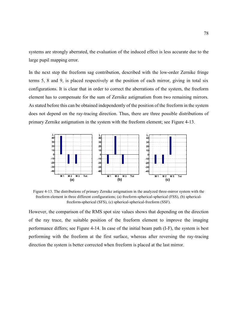
78
systems are strongly aberrated, the evaluation of the induced effect is less accurate due to the
large pupil mapping error.
In the next step the freeform sag contribution, described with the low-order Zernike fringe
terms 5, 8 and 9, is placed respectively at the position of each mirror, giving in total six
configurations. It is clear that in order to correct the aberrations of the system, the freeform
element has to compensate for the sum of Zernike astigmatism from two remaining mirrors.
As stated before this can be obtained independently of the position of the freeform in the system
does not depend on the ray-tracing direction. Thus, there are three possible distributions of
primary Zernike astigmatism in the system with the freeform element; see Figure 4-13.
Figure 4-13. The distributions of primary Zernike astigmatism in the analyzed three-mirror system with the
freeform element in three different configurations; (a) freeform-spherical-spherical (FSS), (b) spherical-
freeform-spherical (SFS), (c) spherical-spherical-freeform (SSF).
However, the comparison of the RMS spot size values shows that depending on the direction
of the ray trace, the suitable position of the freeform element to improve the imaging
performance differs; see Figure 4-14. In case of the initial beam path (I-F), the system is best
performing with the freeform at the first surface, whereas after reversing the ray-tracing
direction the system is better corrected when freeform is placed at the last mirror.
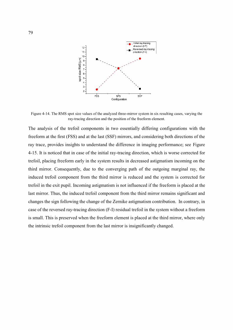
79
Figure 4-14. The RMS spot size values of the analyzed three-mirror system in six resulting cases, varying the
ray-tracing direction and the position of the freeform element.
The analysis of the trefoil components in two essentially differing configurations with the
freeform at the first (FSS) and at the last (SSF) mirrors, and considering both directions of the
ray trace, provides insights to understand the difference in imaging performance; see Figure
4-15. It is noticed that in case of the initial ray-tracing direction, which is worse corrected for
trefoil, placing freeform early in the system results in decreased astigmatism incoming on the
third mirror. Consequently, due to the converging path of the outgoing marginal ray, the
induced trefoil component from the third mirror is reduced and the system is corrected for
trefoil in the exit pupil. Incoming astigmatism is not influenced if the freeform is placed at the
last mirror. Thus, the induced trefoil component from the third mirror remains significant and
changes the sign following the change of the Zernike astigmatism contribution. In contrary, in
case of the reversed ray-tracing direction (F-I) residual trefoil in the system without a freeform
is small. This is preserved when the freeform element is placed at the third mirror, where only
the intrinsic trefoil component from the last mirror is insignificantly changed.
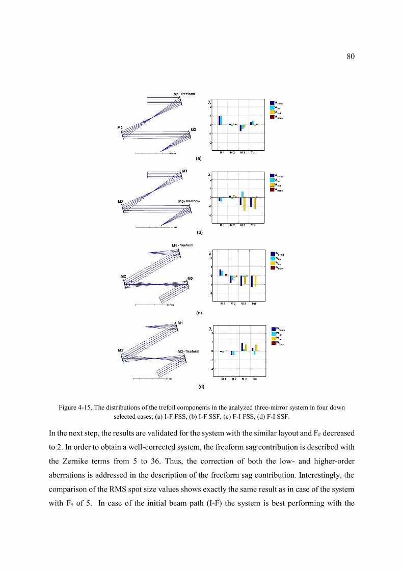
80
Figure 4-15. The distributions of the trefoil components in the analyzed three-mirror system in four down
selected cases; (a) I-F FSS, (b) I-F SSF, (c) F-I FSS, (d) F-I SSF.
In the next step, the results are validated for the system with the similar layout and F# decreased
to 2. In order to obtain a well-corrected system, the freeform sag contribution is described with
the Zernike terms from 5 to 36. Thus, the correction of both the low- and higher-order
aberrations is addressed in the description of the freeform sag contribution. Interestingly, the
comparison of the RMS spot size values shows exactly the same result as in case of the system
with F# of 5. In case of the initial beam path (I-F) the system is best performing with the
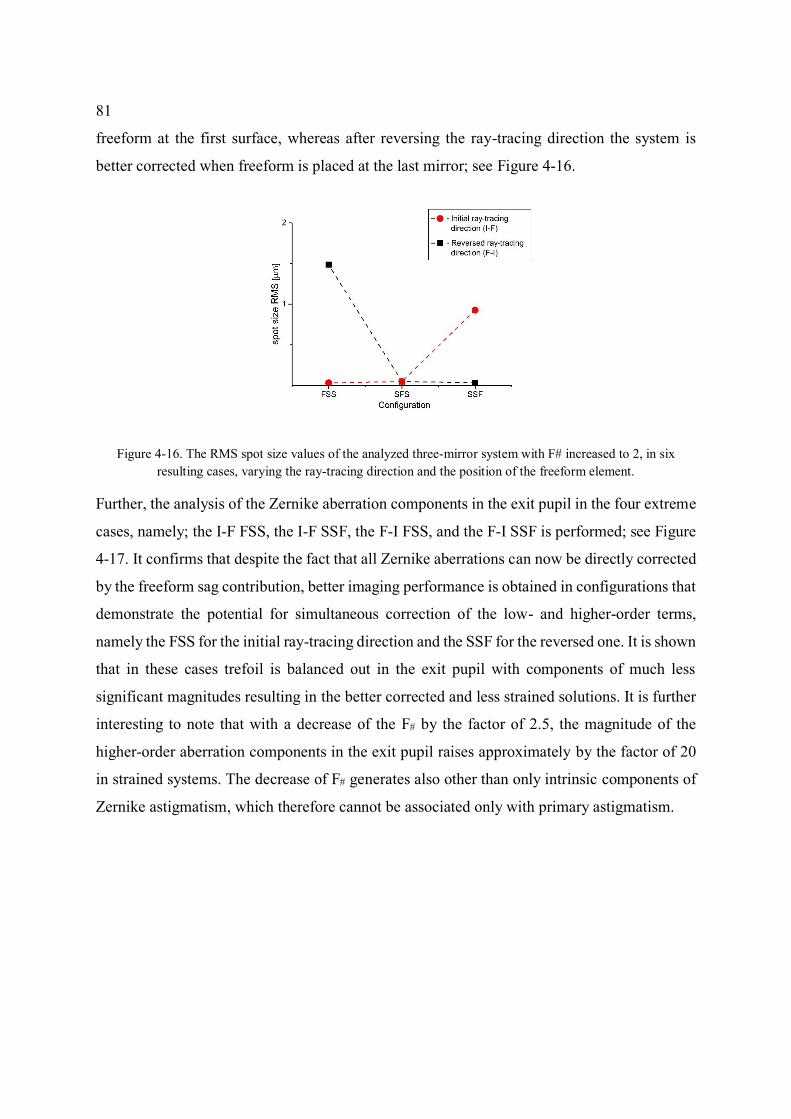
81
freeform at the first surface, whereas after reversing the ray-tracing direction the system is
better corrected when freeform is placed at the last mirror; see Figure 4-16.
Figure 4-16. The RMS spot size values of the analyzed three-mirror system with F# increased to 2, in six
resulting cases, varying the ray-tracing direction and the position of the freeform element.
Further, the analysis of the Zernike aberration components in the exit pupil in the four extreme
cases, namely; the I-F FSS, the I-F SSF, the F-I FSS, and the F-I SSF is performed; see Figure
4-17. It confirms that despite the fact that all Zernike aberrations can now be directly corrected
by the freeform sag contribution, better imaging performance is obtained in configurations that
demonstrate the potential for simultaneous correction of the low- and higher-order terms,
namely the FSS for the initial ray-tracing direction and the SSF for the reversed one. It is shown
that in these cases trefoil is balanced out in the exit pupil with components of much less
significant magnitudes resulting in the better corrected and less strained solutions. It is further
interesting to note that with a decrease of the F# by the factor of 2.5, the magnitude of the
higher-order aberration components in the exit pupil raises approximately by the factor of 20
in strained systems. The decrease of F# generates also other than only intrinsic components of
Zernike astigmatism, which therefore cannot be associated only with primary astigmatism.
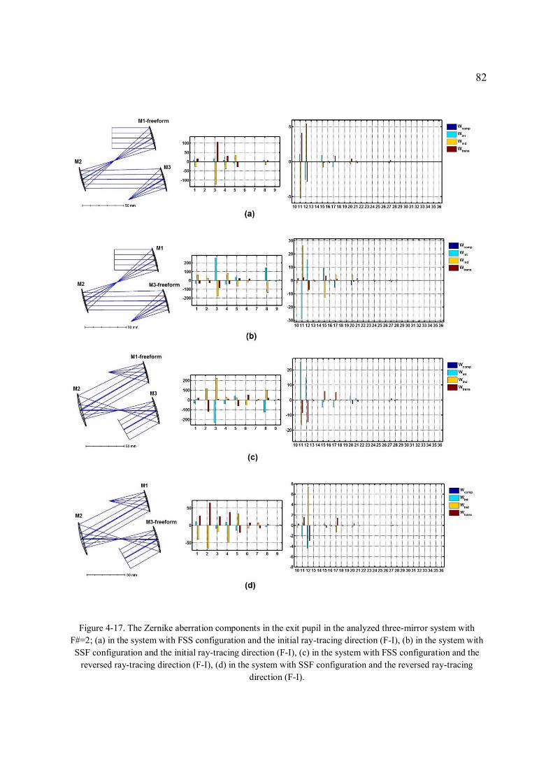
82
Figure 4-17. The Zernike aberration components in the exit pupil in the analyzed three-mirror system with
F#=2; (a) in the system with FSS configuration and the initial ray-tracing direction (F-I), (b) in the system with
SSF configuration and the initial ray-tracing direction (F-I), (c) in the system with FSS configuration and the
reversed ray-tracing direction (F-I), (d) in the system with SSF configuration and the reversed ray-tracing
direction (F-I).
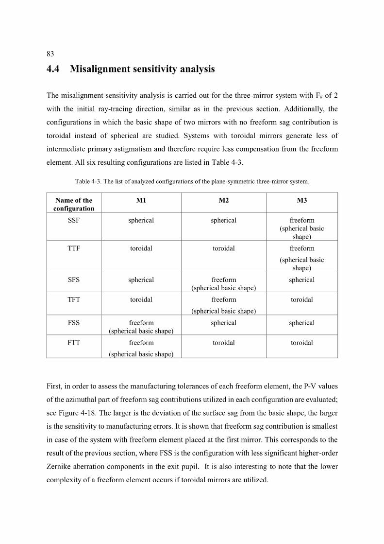
83
4.4 Misalignment sensitivity analysis
The misalignment sensitivity analysis is carried out for the three-mirror system with F# of 2
with the initial ray-tracing direction, similar as in the previous section. Additionally, the
configurations in which the basic shape of two mirrors with no freeform sag contribution is
toroidal instead of spherical are studied. Systems with toroidal mirrors generate less of
intermediate primary astigmatism and therefore require less compensation from the freeform
element. All six resulting configurations are listed in Table 4-3.
Table 4-3. The list of analyzed configurations of the plane-symmetric three-mirror system.
Name of the
configuration
M1 M2 M3
SSF spherical spherical freeform
(spherical basic
shape)
TTF toroidal toroidal freeform
(spherical basic
shape)
SFS spherical freeform
(spherical basic shape)
spherical
TFT toroidal freeform
(spherical basic shape)
toroidal
FSS freeform
(spherical basic shape)
spherical spherical
FTT freeform
(spherical basic shape)
toroidal toroidal
First, in order to assess the manufacturing tolerances of each freeform element, the P-V values
of the azimuthal part of freeform sag contributions utilized in each configuration are evaluated;
see Figure 4-18. The larger is the deviation of the surface sag from the basic shape, the larger
is the sensitivity to manufacturing errors. It is shown that freeform sag contribution is smallest
in case of the system with freeform element placed at the first mirror. This corresponds to the
result of the previous section, where FSS is the configuration with less significant higher-order
Zernike aberration components in the exit pupil. It is also interesting to note that the lower
complexity of a freeform element occurs if toroidal mirrors are utilized.
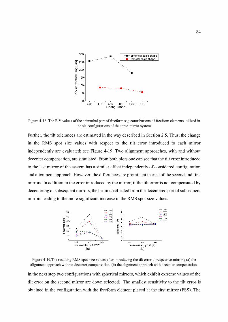
84
Figure 4-18. The P-V values of the azimuthal part of freeform sag contributions of freeform elements utilized in
the six configurations of the three-mirror system.
Further, the tilt tolerances are estimated in the way described in Section 2.5. Thus, the change
in the RMS spot size values with respect to the tilt error introduced to each mirror
independently are evaluated; see Figure 4-19. Two alignment approaches, with and without
decenter compensation, are simulated. From both plots one can see that the tilt error introduced
to the last mirror of the system has a similar effect independently of considered configuration
and alignment approach. However, the differences are prominent in case of the second and first
mirrors. In addition to the error introduced by the mirror, if the tilt error is not compensated by
decentering of subsequent mirrors, the beam is reflected from the decentered part of subsequent
mirrors leading to the more significant increase in the RMS spot size values.
Figure 4-19.The resulting RMS spot size values after introducing the tilt error to respective mirrors; (a) the
alignment approach without decenter compensation, (b) the alignment approach with decenter compensation.
In the next step two configurations with spherical mirrors, which exhibit extreme values of the
tilt error on the second mirror are down selected. The smallest sensitivity to the tilt error is
obtained in the configuration with the freeform element placed at the first mirror (FSS). The
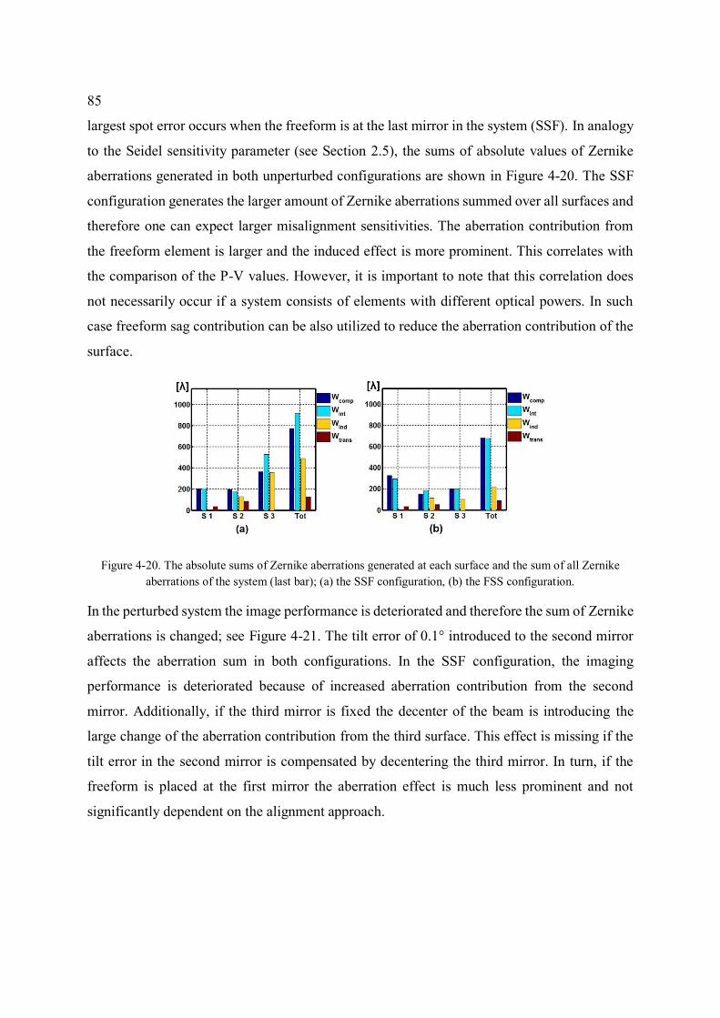
85
largest spot error occurs when the freeform is at the last mirror in the system (SSF). In analogy
to the Seidel sensitivity parameter (see Section 2.5), the sums of absolute values of Zernike
aberrations generated in both unperturbed configurations are shown in Figure 4-20. The SSF
configuration generates the larger amount of Zernike aberrations summed over all surfaces and
therefore one can expect larger misalignment sensitivities. The aberration contribution from
the freeform element is larger and the induced effect is more prominent. This correlates with
the comparison of the P-V values. However, it is important to note that this correlation does
not necessarily occur if a system consists of elements with different optical powers. In such
case freeform sag contribution can be also utilized to reduce the aberration contribution of the
surface.
Figure 4-20. The absolute sums of Zernike aberrations generated at each surface and the sum of all Zernike
aberrations of the system (last bar); (a) the SSF configuration, (b) the FSS configuration.
In the perturbed system the image performance is deteriorated and therefore the sum of Zernike
aberrations is changed; see Figure 4-21. The tilt error of 0.1° introduced to the second mirror
affects the aberration sum in both configurations. In the SSF configuration, the imaging
performance is deteriorated because of increased aberration contribution from the second
mirror. Additionally, if the third mirror is fixed the decenter of the beam is introducing the
large change of the aberration contribution from the third surface. This effect is missing if the
tilt error in the second mirror is compensated by decentering the third mirror. In turn, if the
freeform is placed at the first mirror the aberration effect is much less prominent and not
significantly dependent on the alignment approach.
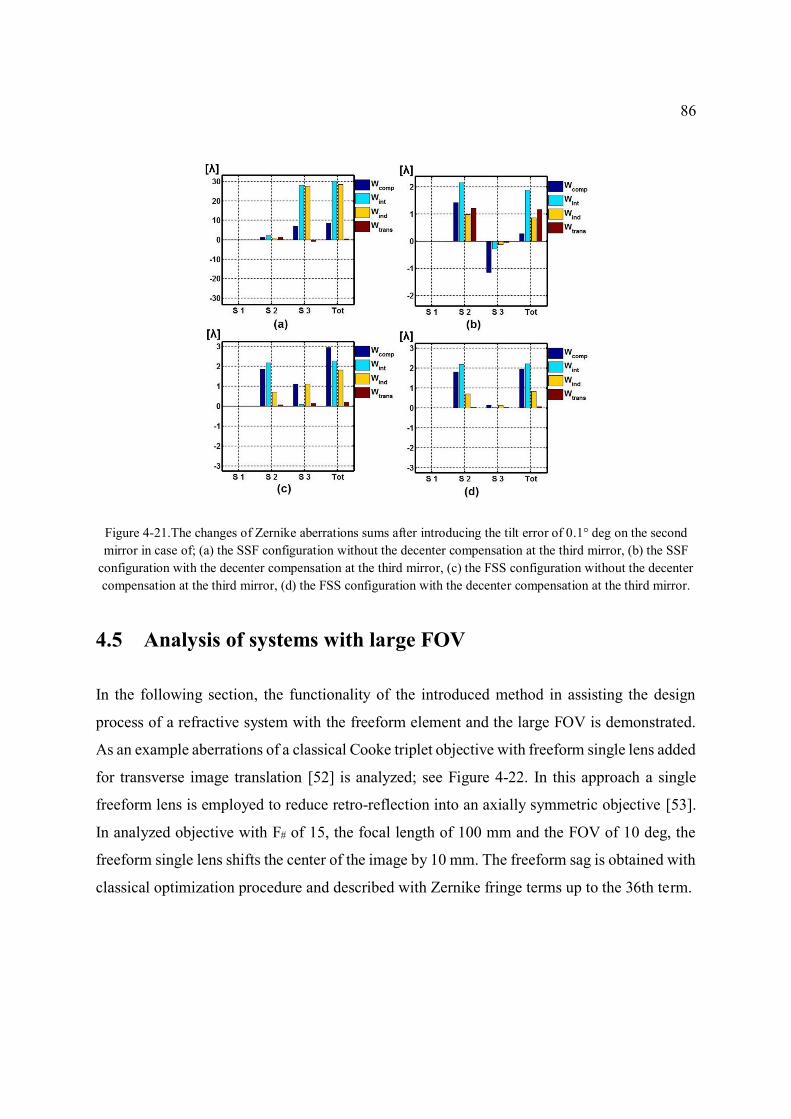
86
Figure 4-21.The changes of Zernike aberrations sums after introducing the tilt error of 0.1° deg on the second
mirror in case of; (a) the SSF configuration without the decenter compensation at the third mirror, (b) the SSF
configuration with the decenter compensation at the third mirror, (c) the FSS configuration without the decenter
compensation at the third mirror, (d) the FSS configuration with the decenter compensation at the third mirror.
4.5 Analysis of systems with large FOV
In the following section, the functionality of the introduced method in assisting the design
process of a refractive system with the freeform element and the large FOV is demonstrated.
As an example aberrations of a classical Cooke triplet objective with freeform single lens added
for transverse image translation [52] is analyzed; see Figure 4-22. In this approach a single
freeform lens is employed to reduce retro-reflection into an axially symmetric objective [53].
In analyzed objective with F# of 15, the focal length of 100 mm and the FOV of 10 deg, the
freeform single lens shifts the center of the image by 10 mm. The freeform sag is obtained with
classical optimization procedure and described with Zernike fringe terms up to the 36th term.
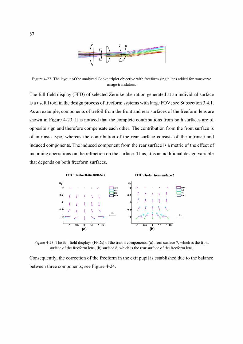
87
Figure 4-22. The layout of the analyzed Cooke triplet objective with freeform single lens added for transverse
image translation.
The full field display (FFD) of selected Zernike aberration generated at an individual surface
is a useful tool in the design process of freeform systems with large FOV; see Subsection 3.4.1.
As an example, components of trefoil from the front and rear surfaces of the freeform lens are
shown in Figure 4-23. It is noticed that the complete contributions from both surfaces are of
opposite sign and therefore compensate each other. The contribution from the front surface is
of intrinsic type, whereas the contribution of the rear surface consists of the intrinsic and
induced components. The induced component from the rear surface is a metric of the effect of
incoming aberrations on the refraction on the surface. Thus, it is an additional design variable
that depends on both freeform surfaces.
Figure 4-23. The full field displays (FFDs) of the trefoil components; (a) from surface 7, which is the front
surface of the freeform lens, (b) surface 8, which is the rear surface of the freeform lens.
Consequently, the correction of the freeform in the exit pupil is established due to the balance
between three components; see Figure 4-24.
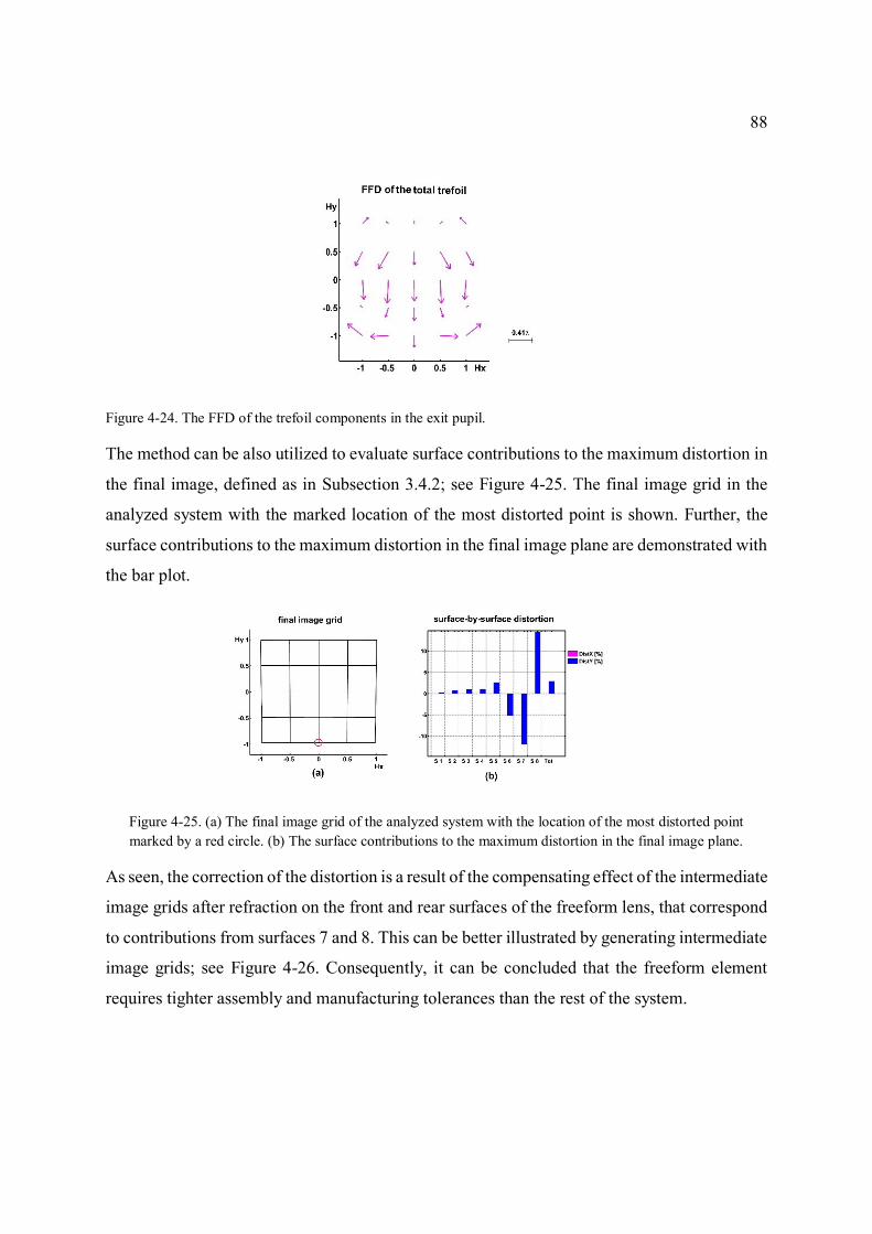
88
Figure 4-24. The FFD of the trefoil components in the exit pupil.
The method can be also utilized to evaluate surface contributions to the maximum distortion in
the final image, defined as in Subsection 3.4.2; see Figure 4-25. The final image grid in the
analyzed system with the marked location of the most distorted point is shown. Further, the
surface contributions to the maximum distortion in the final image plane are demonstrated with
the bar plot.
Figure 4-25. (a) The final image grid of the analyzed system with the location of the most distorted point
marked by a red circle. (b) The surface contributions to the maximum distortion in the final image plane.
As seen, the correction of the distortion is a result of the compensating effect of the intermediate
image grids after refraction on the front and rear surfaces of the freeform lens, that correspond
to contributions from surfaces 7 and 8. This can be better illustrated by generating intermediate
image grids; see Figure 4-26. Consequently, it can be concluded that the freeform element
requires tighter assembly and manufacturing tolerances than the rest of the system.
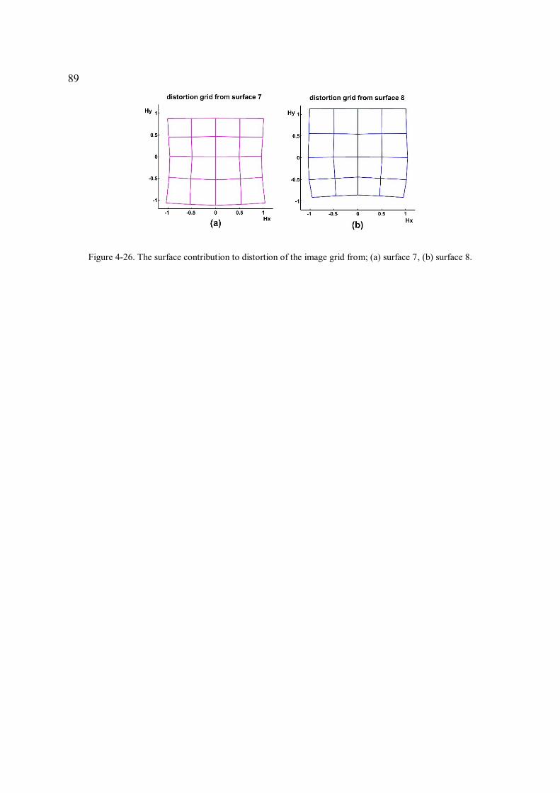
89
Figure 4-26. The surface contribution to distortion of the image grid from; (a) surface 7, (b) surface 8.
90
Chapter 5 Conclusions
In this thesis the novel numerical method for determining surface-by-surface contributions to
the total wave aberration was introduced. It utilizes data from tracing multiple ray sets to
determine surface contribution further divided with respect to phenomenological origin into
intrinsic, induced and transfer components. Each aberration component is determined from a
separate set of rays.
The method provides aberration coefficients derived for a single field point. The graphical
representation of field dependency is possible with full-field displays. In principle no
constraints are placed on the geometry of an analyzed system. However, in this thesis only
plane symmetric freeform systems were studied. Additionally, only systems with near-circular
apertures were considered. This allowed characterizing the obtained aberration components
with Zernike fringe polynomials.
Currently available analytical methods, typically used to analyze wave aberrations are;
coefficients derived from NAT for non-axially symmetric systems and coefficients of the wave
aberration function expanded to the sixth order. Additionally, optical design programs provide
a tool utilizing ray-tracing data to determine the Zernike aberration coefficients in the exit pupil
of the system. The presented approach introduces features supplementary to the existing tools,
summarized in Table 5-1.
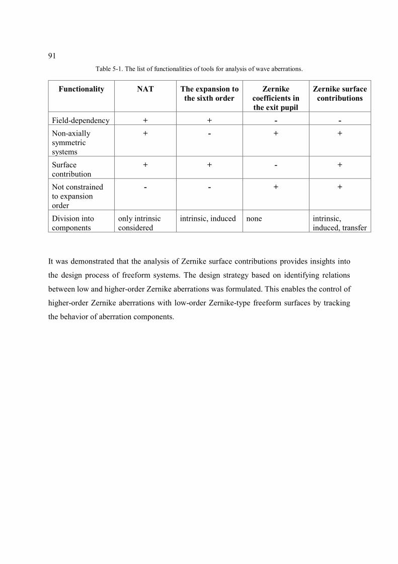
91
Table 5-1. The list of functionalities of tools for analysis of wave aberrations.
Functionality NAT The expansion to
the sixth order
Zernike
coefficients in
the exit pupil
Zernike surface
contributions
Field-dependency + + - -
Non-axially
symmetric
systems
+ - + +
Surface
contribution
+ + - +
Not constrained
to expansion
order
- - + +
Division into
components
only intrinsic
considered
intrinsic, induced none intrinsic,
induced, transfer
It was demonstrated that the analysis of Zernike surface contributions provides insights into
the design process of freeform systems. The design strategy based on identifying relations
between low and higher-order Zernike aberrations was formulated. This enables the control of
higher-order Zernike aberrations with low-order Zernike-type freeform surfaces by tracking
the behavior of aberration components.
92
Appendix A
Performance comparison of methods allowing for
communication between Matlab® and Zemax®
A.1 Possible methods
Presented is the performance comparison of COM and DDE protocols, which allow for two-
way communication between Matlab® and Zemax®. Both are applicable with the toolboxes
MZCOM (by Norman G. Worku) and MZDDE (by D.Griffith). First is introduced for versions
of Zemax® starting with OpticStudio15®, latter is supported for all professional Zemax®
versions. COM works only for 64 bit versions of Matlab® whereas DDE works uninterrupted
for 32 bit version experiencing connection breaks when used with 64 bit version. Additionally
two modes for utilizing COM protocol are compared. The interactive mode placing changes to
the currently opened copy of OpticStudio15® and standalone mode that creates the copy of the
file in Matlab® (occupies license key) and operates on it.
Firstly, methods are tested for time efficiency in modifying a lens file from Matlab®. Secondly,
to find the efficient way for transferring the ray-tracing data of larger number of rays into
Matlab® workspace, the COM routine BatchArrayTrace is compared against zArrayTrace
.mex file* based on DDE protocol. Finally, combined approaches for two-way communication
are tested. These are COM in standalone mode, COM in interactive mode together with .mex64
file and DDE with .mex32. All methods are tested for their speed in exchanging the data
between two programs.
* mex files are functions written in C, compiled to be compatible with MATLAB environment.
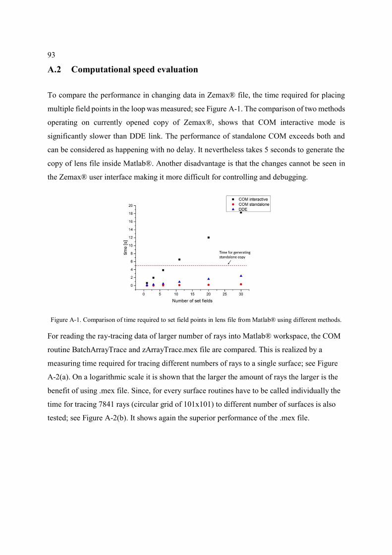
93
A.2 Computational speed evaluation
To compare the performance in changing data in Zemax® file, the time required for placing
multiple field points in the loop was measured; see Figure A-1. The comparison of two methods
operating on currently opened copy of Zemax®, shows that COM interactive mode is
significantly slower than DDE link. The performance of standalone COM exceeds both and
can be considered as happening with no delay. It nevertheless takes 5 seconds to generate the
copy of lens file inside Matlab®. Another disadvantage is that the changes cannot be seen in
the Zemax® user interface making it more difficult for controlling and debugging.
Figure A-1. Comparison of time required to set field points in lens file from Matlab® using different methods.
For reading the ray-tracing data of larger number of rays into Matlab® workspace, the COM
routine BatchArrayTrace and zArrayTrace.mex file are compared. This is realized by a
measuring time required for tracing different numbers of rays to a single surface; see Figure
A-2(a). On a logarithmic scale it is shown that the larger the amount of rays the larger is the
benefit of using .mex file. Since, for every surface routines have to be called individually the
time for tracing 7841 rays (circular grid of 101x101) to different number of surfaces is also
tested; see Figure A-2(b). It shows again the superior performance of the .mex file.
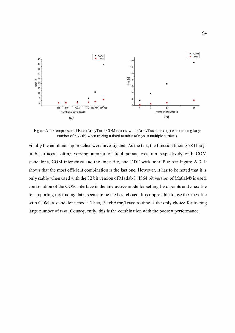
94
Figure A-2. Comparison of BatchArrayTrace COM routine with zArrayTrace.mex; (a) when tracing large
number of rays (b) when tracing a fixed number of rays to multiple surfaces.
Finally the combined approaches were investigated. As the test, the function tracing 7841 rays
to 6 surfaces, setting varying number of field points, was run respectively with COM
standalone, COM interactive and the .mex file, and DDE with .mex file; see Figure A-3. It
shows that the most efficient combination is the last one. However, it has to be noted that it is
only stable when used with the 32 bit version of Matlab®. If 64 bit version of Matlab® is used,
combination of the COM interface in the interactive mode for setting field points and .mex file
for importing ray tracing data, seems to be the best choice. It is impossible to use the .mex file
with COM in standalone mode. Thus, BatchArrayTrace routine is the only choice for tracing
large number of rays. Consequently, this is the combination with the poorest performance.
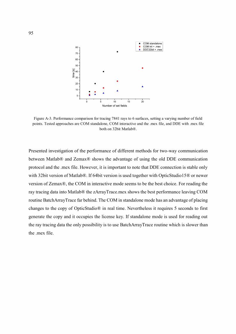
95
Figure A-3. Performance comparison for tracing 7841 rays to 6 surfaces, setting a varying number of field
points. Tested approaches are COM standalone, COM interactive and the .mex file, and DDE with .mex file
both on 32bit Matlab®.
Presented investigation of the performance of different methods for two-way communication
between Matlab® and Zemax® shows the advantage of using the old DDE communication
protocol and the .mex file. However, it is important to note that DDE connection is stable only
with 32bit version of Matlab®. If 64bit version is used together with OpticStudio15® or newer
version of Zemax®, the COM in interactive mode seems to be the best choice. For reading the
ray tracing data into Matlab® the zArrayTrace.mex shows the best performance leaving COM
routine BatchArrayTrace far behind. The COM in standalone mode has an advantage of placing
changes to the copy of OpticStudio® in real time. Nevertheless it requires 5 seconds to first
generate the copy and it occupies the license key. If standalone mode is used for reading out
the ray tracing data the only possibility is to use BatchArrayTrace routine which is slower than
the .mex file.

References
1. Gross, H., Blechinger, F., Achtner, B., Handbook of Optical Systems, Vol. 4, 2008: Wiley-
VCH.
2. Cruickshank, F.D. and G.A. Hills, Use of Optical Aberration Coefficients in Optical Design,
Journal of the Optical Society of America, 1960. 50(4): p. 379-387.
3. Welford, W.T., Aberrations in optical systems, 1986: Taylor & Francis.
4. Meiron, J., Damped Least-Squares Method for Automatic Lens Design, Journal of the Optical
Society of America, 1965. 55(9): p. 1105-1109.
5. Dilworth, D.C., Pseudo-second-derivative matrix and its application to automatic lens design,
Applied Optics, 1978. 17(21): p. 3372-3375.
6. Isshiki, M., Ono, H., Hiraga, K. et al., Lens Design: Global Optimization with Escape
Function, OPT REV, 1995. 2(6): p. 463-470.
7. Chen, X. and K. Yamamoto, An experiment in genetic optimization in lens design, Journal of
Modern Optics, 1997. 44(9): p. 1693-1702.
8. van Turnhout, M., et al., Obtaining new local minima in lens design by constructing saddle
points, Optics Express, 2015. 23(5): p. 6679-6691.
9. Menke, C., Application of particle swarm optimization to the automatic design of optical
systems, SPIE Proc., 2018. 10690: p.10.
10. Sasián, J., Theory of sixth-order wave aberrations, Applied Optics, 2010. 49(33): p. 6502-
6503.
11. Sasian, J., How to approach the design of a bilateral symmetric optical system, Optical
Engineering, 1994. 33(6): p. 2045-2061.
12. Thompson, K., Description of the third-order optical aberrations of near-circular pupil
optical systems without symmetry, Journal of the Optical Society of America A, 2005. 22(7):
p. 1389-1401.
13. Sasian, J., Extrinsic aberrations in optical imaging systems, Adv. Opt. Techn, 2013. 2(1):
p.75-80
14. Bentley, J.L., C. Olson, and R.N. Youngworth, In the era of global optimization, the
understanding of aberrations remains the key to designing superior optical systems, SPIE
Proc., 2010. 7849: p. 13.
15. Fuerschbach, K., J.P. Rolland, and K.P. Thompson, A new family of optical systems
employing φ-polynomial surfaces. Optics Express, 2011. 19(22): p. 21919-21928.
16. Gross, H., et al., Overview on surface representations for freeform surfaces, SPIE Poc., 2015.
9626: p. 14.
17. Forbes, G.W., Characterizing the shape of freeform optics, Optics Express, 2012. 20(3): p.
2483-2499.
18. Broemel, A., Lippmann, U., Gross, H., Freeform surface descriptions - part I: Mathematical
representations, Adv. Opt. Techn., 2017. 6(5): p. 327-336
19. Broemel, A., Liu, C., Zhang, Y., Zhang, Y., Gross, H., Freeform surface descriptions. Part II:
Application benchmark, Adv. Opt. Techn., 2017. 6(5): p.337-347.
20. Stock, J., et al., Description and reimplementation of real freeform surfaces, Applied Optics,
2017. 56(3): p. 391-396.
21. Liu, C. and H. Gross, Numerical optimization strategy for multi-lens imaging systems
containing freeform surfaces, Applied Optics, 2018. 57(20): p. 5758-5768.
22. Bauer, A., E.M. Schiesser, and J.P. Rolland, Starting geometry creation and design method
for freeform optics, Nature Communications, 2018. 9(1): p. 1756.
23. Fuerschbach, K., J.P. Rolland, and K.P. Thompson, Theory of aberration fields for general
optical systems with freeform surfaces, Optics Express, 2014. 22(22): p. 26585-26606.
24. Zhong, Y. and H. Gross, Initial system design method for non-rotationally symmetric systems
based on Gaussian brackets and Nodal aberration theory, Optics Express, 2017. 25(9): p.
10016-10030.
25. Sasián, J., Aberrations in optical imaging systems, 2013: Cambridge Press.
26. Hopkins, H.H., Wave Theory of Aberrations, 1950: Clarendon Press.
27. Sasian, J., Design Of Null Lens Correctors For The Testing Of Astronomical Optics, SPIE
Proc., 1988. 27: p. 6.
28. Hoffman, J.M., Induced aberrations in optical systems, Ph.D. Thesis, 1993, The University of
Arizona.
29. Sasián, J., Theory of sixth-order wave aberrations: errata, Applied Optics, 2010. 49(16): p.
D69-D95.
30. Buchroeder, R.A., Tilted component optical systems, Ph.D. Thesis, 1976, The University of
Arizona.
31. Thompson, K.P., et al., Using nodal aberration theory to understand the aberrations of
multiple unobscured three mirror anastigmatic (TMA) telescopes, SPIE Proc., 2009. 7433:
p.8.
32. Moore, L.B., A.M. Hvisc, and J. Sasian, Aberration fields of a combination of plane
symmetric systems, Optics Express, 2008. 16(20): p. 15655-15670.
33. Gross, H., Handbook of Optical Systems, Vol. 1, 2004: WILEY-VCH.
34. Hopkins, H.H., Canonical Pupil Coordinates in Geometrical and Diffraction Image Theory,
Japanese Journal of Applied Physics, 1964. 3(S1): p. 31.
35. Hopkins, G.W., Aberrational analysis of optical systems: a proximate ray trace approach,
1976, The University of Arizona.
36. Weinstein, W., Wave-front Aberrations of Oblique Pencils in a Symmetrical Optical System:
Refraction and Transfer Formulae, Proceedings of the Physical Society. Section B, 1949.
62(11): p. 726.
37. Gross, H. and C. Liu, Generalized Surface Aberration Contributions, Paper presented at
EOSAM. 2014: Berlin.
38. Walther, A., The Ray and Wave Theory of Lenses, 1995: Cambridge University Press.
39. Gross, H., Zügge, H., Peschka, M., Blechinger, F., Handbook of Optical Systems, Vol. 3,
2007: WILEY-VCH.
40. Zemax LLC, User's Manual. 2015.
41. Ruoff, J. and M. Totzeck, Orientation Zernike polynomials: a useful way to describe the
polarization effects of optical imaging systems, Journal of Micro/Nanolithography, MEMS,
and MOEMS, 2009. 8(3), 031404: p. 22.
42. Agurok, I.y.P., Double expansion of wavefront deformation in Zernike polynomials over the
pupil and the field of view of optical systems: lens design, testing, and alignment, SPIE Proc.,
1998. 3430: p. 8.
43. Lundström, L. and P. Unsbo, Transformation of Zernike coefficients: scaled, translated, and
rotated wavefronts with circular and elliptical pupils, Journal of the Optical Society of
America A, 2007. 24(3): p. 569-577.
44. Forbes, G.W., Shape specification for axially symmetric optical surfaces, Optics Express,
2007. 15(8): p. 5218-5226.
45. Forbes, G.W., Fitting freeform shapes with orthogonal bases, Optics Express, 2013. 21(16):
p. 19061-19081.
46. Dilworth, D.C., New tools for the lens designer, SPIE Proc., 2008. 7060, p. 10.
47. Musick, D.J., Investigation of Desensitization Methods for High-Resolution Endoscopes,
2016, Master Thesis, Friedrich-Schiller-Universität Jena.
48. Oleszko, M., R. Hambach, and H. Gross, Decomposition of the total wave aberration in
generalized optical systems, Journal of the Optical Society of America A, 2017. 34(10): p.
1856-1864.
49. Zhu, S., Full field aberration representation, 2016, Internal Report, Friedrich-Schiller-
Universität Jena.
50. Rodgers, J.M., Unobscured mirror designs, SPIE Proc., 2002. 4832: p. 28.
51. Oleszko, M. and H. Gross, Analysis of freeform mirror systems based on the decomposition of
the total wave aberration into Zernike surface contributions, Applied Optics, 2018. 57(9): p.
1998-2006.
52. Wu, X., et al., Transverse image translation using an optical freeform single lens, Applied
Optics, 2015. 54(28): p. E55-E62.
53. He, S., Y. Meng, and M. Gong, Freeform lens design to eliminate retroreflection for optical
systems, Applied Optics, 2018. 57(5): p. 1218-1224.

Acknowledgements
This research was partially founded by the German Federal Ministry of Education and Research
with the project fo+ (FKZ: 03WKCK1D).
I would like to thank Prof. Herbert Gross for giving me the opportunity to work on the topic of
wave aberrations to which I was keen to contribute and for the possibility to participate in
international conferences.
I also acknowledge again my supervisor Prof. Herbert Gross and Dr. Ralf Hambach for help in
formulating the ideas of this thesis through many scientific discussions.
Thanks to my great officemate Christoph Bösel. I have appreciated all of our discussions and
companionship throughout the years. I am grateful to my group members for creating a pleasant
working atmosphere occasionally distracted by sharing a piece of cake.
I would like to thank my classmates from Master in Photonics Program who were the people I
first met after coming to Jena, especially; Can Boran Akdal, Dr. Lorenz von Grafenstein,
Franck Gounou, Dr. Samuel Serna.
I would also like to thank numerous fellow scientists scattered around the Beutenberg campus
for their friendship; Dr. Pol Ribes, Sophie Sauva, Dr. Lilia Espada, Dr. Pol Alonso, Lorena
Halty, Dr. Oscar Gutierrez, Dr. Ilona Koebsch, Dr. Rossa Mac Ciarnain, Marta Kazimierska,
Tobias Tieß, Agnieszka Litomska, Asya Martirosyan, Sean Garnsey, Marta Gilaberte, Dr. Shu
Zhe, Florencia Campetella, Aoife Brady and many others who I met during the time of my Phd
work. In particular, I would like to thank Laura Keys for her companionship and understanding.
And lastly, I am grateful to; my parents, sister Dorota and cousin Lukasz, with his wife Asia,
and to my oldest niece Lena for their unconditional support that has contributed to the
completion of this thesis.

This page is left blank intentionally.
Zusammenfassung
Die zunehmende Verwendung von optischen Freiformflächen erhöht die Forderung nach
optischen Designwerkzeugen die für allgemeine Systeme entwickelt wurden. Im Design-
Prozess sind oberflächenbedingte Aberrationsbeiträge von besonderem Interesse. Die
Erweiterung der Wellenaberrationsfunktion in feld- und pupillen-abhängige Koeffizienten ist
eine zu diesem Zweck verwendete analytische Methode. Ein alternativer numerischer Ansatz,
der Daten aus der Verlauf von mehreren Strahlenbündeln verwendet, wird vorgeschlagen. Das
optische System ist in Segmente des optischen Weges unterteilt, die entlang des Hauptstrahls
gemessen werden. Oberflächenbeiträge repräsentieren die Änderung der Wellenfront, die
aufgrund der Propagation durch einzelne Segmente auftritt. Ferner sind die
Oberflächenbeiträge hinsichtlich ihres phänomenologischen Ursprungs in intrinsische
induzierte und transferierende Komponenten unterteilt. Jede Komponente wird aus einem
separaten Strahlenbündel bestimmt. Die vorgeschlagene Methode stellt keine Beschränkungen
für die Systemgeometrie oder die Apertur bereit. In dieser Arbeit werden jedoch nur ebene
symmetrische Systeme mit nahezu kreisförmigen Aperturen untersucht. Dies ermöglichte eine
Charakterisierung der erhaltenen Aberrationskomponenten mit Zernike-Randpolynomen.
Die Anwendung der vorgeschlagenen Methode im Designprozess der Freiformsysteme wird
demonstriert. Die Analyse der Zernike-Oberflächenbeiträge liefert wertvolle Erkenntnisse für
die Auswahl des Startsystems mit dem besten Potenzial zur Korrektur von Aberrationen mit
Freiformflächen. Außerdem hilft es beim Bestimmen der effektiven Position eines
Freiformelements in einem System. Folglich ist es möglich, Systeme zu entwerfen, die für
Zernike-Aberrationen höherer Ordnung korrigiert sind als die für die Freiform-Sag Beiträge
verwendeten Koeffizienten, die mit demselben Zernike-Polynomsatz beschrieben sind.

This page is left blank intentionally.
Curriculum Vitae
Oleszko, Mateusz
Date of birth: 10.07.1988
Location of birth: Opole, Poland
09.1995 – 07.2001 Public Primary School No. 14, Opole, Poland
09.2001 – 07.2004 Public Middle School No. 9, Opole, Poland
09.2004 – 04.2007 Secondary Education Public High School No. 3, Opole, Poland
10.2007 – 01.2011 Bachelor of Engineering Politechnika Wroclawska, Wroclaw, Poland
in Applied Physics
02.2010 – 07.2010 Erasmus Exchange Vrije Universiteit Brussel, Brussels, Belgium
10.2011 – 04.2014 Master of Science Friedrich-Schiller-Univerität, Jena, Germany
in Photonics
07.2014 – 08.2018 Ph.D. Candidate Institut für Angewandte Physik, Friedrich-Schiller-
Univerität, Jena, Germany
Jena, 05.11.2018
Signature

This page is left blank intentionally.
Publications
Journal articles
• M. Oleszko and H. Gross, Analysis of freeform mirror systems based on the
decomposition of the total wave aberration into Zernike surface contributions,
Applied Optics, 2018. 57(9): p. 1998-2006.
• M. Oleszko, R. Hambach, and H. Gross, Decomposition of the total wave aberration
in generalized optical systems, Journal of the Optical Society of America A, 2017.
34(10): p. 1856-1864.
Conference proceedings
• M. Oleszko and H. Gross, Zernike surface contributions as an assisting tool for
designing freeform optical systems, SPIE Proc., 2018. 10690: p.9
• M. Oleszko and H. Gross, Generalized surface contributions for misalignment
sensitivity analysis, SPIE Proc., 2017. 10377: p.8
• H. Gross, A. Brömel, M. Beier, R. Steinkopf, J. Hartung, M. Oleszko, D. Ochse,
Overview on surface representations for freeform surfaces, SPIE Proc., 2015. 9626:
p.14
• A. Brömel, H. Gross, D. Ochse, U. Lippmann, C. Ma, Y. Zhong, M. Oleszko,
Performance comparison of polynomial representations for optimizing optical
freeform systems, SPIE Proc., 2015. 9626: p.12

This page is left blank intentionally.
Ehrenwörtliche Erklärung
Ich erkläre hiermit ehrenwörtlich, dass ich die vorliegende Arbeit selbständig, ohne unzulässige Hilfe Dritter
und ohne Benutzung anderer als der angegebenen Hilfsmittel und Literatur angefertigt habe. Die aus anderen
Quellen direkt oder indirekt übernommenen Daten und Konzepte sind unter Angabe der Quelle gekennzeichnet.
Bei der Auswahl und Auswertung folgenden Materials haben mir die nachstehend aufgeführten Personen in der
jeweils beschriebenen Weise unentgeltlich geholfen:
• Herbert Gross, Betreuer.
Weitere Personen waren an der inhaltlich-materiellen Erstellung der vorliegenden Arbeit nicht beteiligt.
Insbesondere habe ich hierfür nicht die entgeltliche Hilfe von Vermittlungs- bzw. Beratungsdiensten
(Promotionsberater oder andere Personen) in Anspruch genommen. Niemand hat von mir unmittelbar oder
mittelbar geldwerte Leistungen für Arbeiten erhalten, die im Zusammenhang mit dem Inhalt der vorgelegten
Dissertation stehen.
Die Arbeit wurde bisher weder im In- noch im Ausland in gleicher oder ähnlicher Form einer anderen
Prüfungsbehörde vorgelegt.
Die geltende Promotionsordnung der Physikalisch-Astronomischen Fakultät ist mir bekannt.
Ich versichere ehrenwörtlich, dass ich nach bestem Wissen die reine Wahrheit gesagt und nichts verschwiegen
habe.
Jena, 05.11.2018
Unterschrift d. Verfassers