Analysis of Government Spending on Agriculture Sector and

“Analysis of Government Spending on Agriculture Sector and its

Effects on Economic Growth in Rwanda”

By Bernard HARERIMANA

College of Business and Economics; (CBE)

School of Economics

MSc. of Science in Economics

Academic Year: 2014-2016

Kigali, June 2016

ii

College of Business and Economics; (CBE)

P.O BOX 1514 KIGALI, RWANDA

GIKONDO Campus

Analysis of Government Spending on Agriculture Sector andits Effects on

Economic Growth in Rwanda

Bernard HARERIMANA

Registration Number: 215033336

A Thesis submitted to the University of Rwanda-College of Business and Economics (CBE) in partial

fulfilment of the academic requirements for the award of Degree of

MASTERS OF SCIENCE IN ECONOMICS

In the college of College of Business and Economics; (CBE)

MASTERS PROGRAM (BATCH V)

Academic Year: 2014-2016

Tutor: Professor Almas Heshmati;

Kigali, June 2016

iii

DEDICATIONS

Allow me to extend my dedications:

To Almighty God,

My Mum

To my Supervisor,

And finally special dedications to all my family and relatives, Brothers and Sisters, to whom I

owe opportunities to attain the MSc. Education level.

iv

DECLARATION

v

AUTHORIZATION FOR SUBMISSION

vi

AKNOWLEDGEMENTS

The Author of the present work would like to accord thanks to the institutions provided data

during the conduct of this research namely NISR, MINECOFIN and MINAGRI

Special thanks to all those who worked tersely and contributed to the success of this work. We

appreciate, wise counsels by the tutor of the thesis Prof. Almas HESHMATI, from the Jӧnkӧping

International Business School (JBIS) of theJӧnkӧping University.

I acknowledge the inputs provided by panellists namely Dr. NDEMEZO Etienne and Dr.

MUTEMBEREZI Fidele during the defending of this thesis held on 24th

June 2016. The advice

was duly noted for future conduct or research activities and comments were gratefully received

and integrated into this document.

I acknowledge efforts from the Planning departments that assisted for over four months to get

required data to accomplish thework, hereby recognizing the Director General of Strategic

Planning in MINAGRI, Dr. Octave SEMWAGA, the Planning and Budget Specialist in

MINAGRI; Mr. Sosthene NDIKUMANA, and Monitoring and Evaluation Specialist Mr. Joas

TUGIZIMANA in the same Ministry. Mr. BIZIMANA Claude, Coordinator of the Rwanda

SAKSS, a Strategic Analysis and Knowledge Support System (SAKSS) node for monitoring and

evaluation of CAADP investment programs. Mr. RUGAJU Theophile and Mr.

NTAKIRUTIMANA Corneille who works in RAB and NAEB respectively as the directors of

Planning.

Staff in the National Budget and National Development Planning departments in MINECOFIN

includingMr. Eric HAKIZIMANA and Mr. John Bosco MUTABAZI and entire team of staff

workmates at the Ministry of Finance and Economic Planning (MINECOFIN-Rwanda)

I am thankful also to my family represented by my Mum NYIRAMBABARIYE Léocadie, my

Sister KWIZERA Solange and my girlfriend DUSHIMIYIMANA JeannetteKAGENZA for their

encouragements and valuable support, without whose unfailing support and best wishes to me

along the Masters studies, I would not have completed the work.

vii

ABSTRACT

The purpose of this of this study is to investigate the effect of government spending on

agriculture (GEA) sector and its contribution to Rwanda’s economic growth. Rwanda has

achieved strong and sustained growth since 2000s, its economy has changed gradually over the

past years and has expanded at an average annual growth rate of more than 7% and on average of

8.2%, from 2008 to 2012. Large agricultural output, although Agriculture contribution to GDP

has declined, agriculture sector remains the core contributor of the economy, with one-third of

the GDP, the production of food crops have been identified as one important contributing factor

led to tremendous socio-economic achievements, in addition to robust exports and strong

domestic demand. This study intends to analyze the effect of government expenditure on

agriculture sector towards boosting economic growth. Using panel data analysis tools EViews

for Rwanda country from 1997 to 2014 sourced from the Ministry of Finance and Economic

Planning (MINECOFIN) and the National Institute of Statistic of Rwanda (NISR), a model and

expanded equation was estimated seeking to quantify the effect of government expenditures for

agricultural development and impact to GDP. The results indicated that government expenditure

on agriculture sector has significant and positive effect where the results show that in the long

run, government expenditures on agriculture explains GDP growth. Ordinary Least Squares,

(OLS) estimates shown that the coefficient for Government Spending on Agriculture (GEA) was

estimated that it is statistically significant. In sum, a 1 unit increase in government spending on

agriculture was found associated with almost 3% effect (2.5%) increase in GDP.

Keywords: Agriculture, Agricultural growth, government spending, Economic growth, OLS,

Rwanda.

JEL Classification Codes:O13; Q14; Q18; C23.

viii

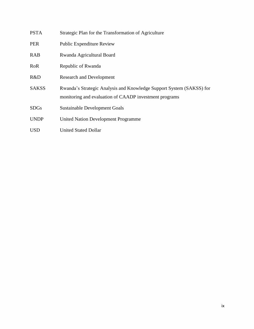
LIST OF SYMBOLS AND ABBREVIATIONS

AgGDP Agricultural Gross Domestic Product

AfDB African Development Bank

ASIP Rwanda’s Agriculture Sector Investment Plan

CAADP Comprehensive Africa Agriculture Development Programme

CIP Crop Intensification Programme

COFOG Classification of Functions of Government

EICV Rwanda Integrated Household Living Conditions Survey

EDPRS Economic Development and Poverty Reduction Strategy

EAC East African Community

Frw Rwandan Franc

GEA Government Expenditure on Agriculture

GMM General Method of Moments

GoR Government of Rwanda

IFPRI International Food Policy Research Institute

IMF International Monetary Fund

MINAGRI Rwanda’s Ministry of Agriculture and Animal Resources

MINECOFIN Rwanda’s Ministry of Finance and Economic Planning

NAEB National Agricultural Export Board

NEPAD The New Partnership for Africa’s Development, A Program of the Africa

NISR National Institute of Statistics of Rwanda

OLS Ordinary Least Squares

ICT Information and Communications Technology

ix

PSTA Strategic Plan for the Transformation of Agriculture

PER Public Expenditure Review

RAB Rwanda Agricultural Board

RoR Republic of Rwanda

R&D Research and Development

SAKSS Rwanda’s Strategic Analysis and Knowledge Support System (SAKSS) for

monitoring and evaluation of CAADP investment programs

SDGs Sustainable Development Goals

UNDP United Nation Development Programme

USD United Stated Dollar

x

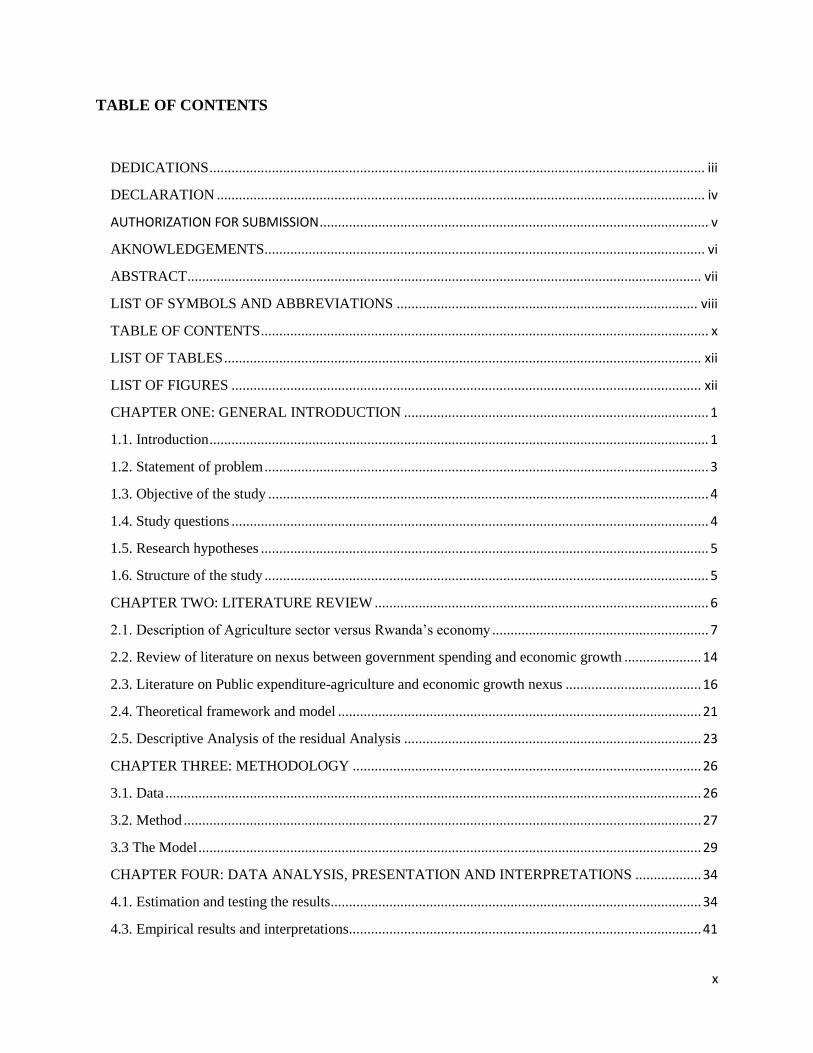
TABLE OF CONTENTS

DEDICATIONS ....................................................................................................................................... iii

DECLARATION ..................................................................................................................................... iv

AUTHORIZATION FOR SUBMISSION .......................................................................................................... v

AKNOWLEDGEMENTS ........................................................................................................................ vi

ABSTRACT ............................................................................................................................................ vii

LIST OF SYMBOLS AND ABBREVIATIONS .................................................................................. viii

TABLE OF CONTENTS .......................................................................................................................... x

LIST OF TABLES .................................................................................................................................. xii

LIST OF FIGURES ................................................................................................................................ xii

CHAPTER ONE: GENERAL INTRODUCTION ................................................................................... 1

1.1. Introduction ........................................................................................................................................ 1

1.2. Statement of problem ......................................................................................................................... 3

1.3. Objective of the study ........................................................................................................................ 4

1.4. Study questions .................................................................................................................................. 4

1.5. Research hypotheses .......................................................................................................................... 5

1.6. Structure of the study ......................................................................................................................... 5

CHAPTER TWO: LITERATURE REVIEW ........................................................................................... 6

2.1. Description of Agriculture sector versus Rwanda’s economy ........................................................... 7

2.2. Review of literature on nexus between government spending and economic growth ..................... 14

2.3. Literature on Public expenditure-agriculture and economic growth nexus ..................................... 16

2.4. Theoretical framework and model ................................................................................................... 21

2.5. Descriptive Analysis of the residual Analysis ................................................................................. 23

CHAPTER THREE: METHODOLOGY ............................................................................................... 26

3.1. Data .................................................................................................................................................. 26

3.2. Method ............................................................................................................................................. 27

3.3 The Model ......................................................................................................................................... 29

CHAPTER FOUR: DATA ANALYSIS, PRESENTATION AND INTERPRETATIONS .................. 34

4.1. Estimation and testing the results ..................................................................................................... 34

4.3. Empirical results and interpretations ................................................................................................ 41

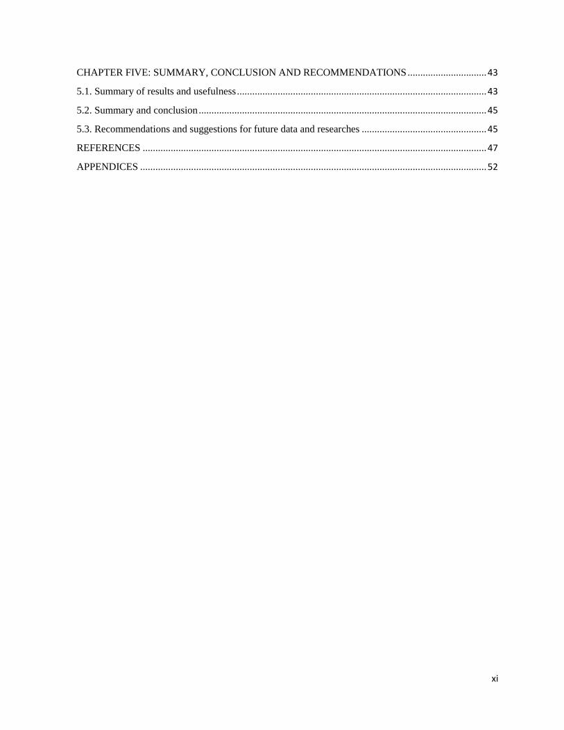
xi

CHAPTER FIVE: SUMMARY, CONCLUSION AND RECOMMENDATIONS ............................... 43

5.1. Summary of results and usefulness .................................................................................................. 43

5.2. Summary and conclusion ................................................................................................................. 45

5.3. Recommendations and suggestions for future data and researches ................................................. 45

REFERENCES ....................................................................................................................................... 47

APPENDICES ........................................................................................................................................ 52

xii

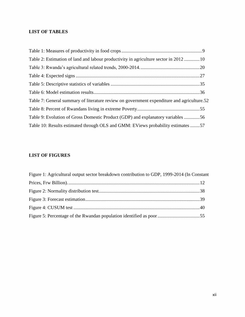
LIST OF TABLES

Table 1: Measures of productivity in food crops ................................................................... 9

Table 2: Estimation of land and labour productivity in agriculture sector in 2012 ............. 10

Table 3: Rwanda’s agricultural related trends, 2000-2014. ................................................. 20

Table 4: Expected signs ....................................................................................................... 27

Table 5: Descriptive statistics of variables .......................................................................... 35

Table 6: Model estimation results ........................................................................................ 36

Table 7: General summary of literature review on government expenditure and agriculture.52

Table 8: Percent of Rwandans living in extreme Poverty .................................................... 55

Table 9: Evolution of Gross Domestic Product (GDP) and explanatory variables ............. 56

Table 10: Results estimated through OLS and GMM: EViews probability estimates ........ 57

LIST OF FIGURES

Figure 1: Agricultural output sector breakdown contribution to GDP, 1999-2014 (In Constant

Prices, Frw Billion). ............................................................................................................. 12

Figure 2: Normality distribution test.................................................................................... 38

Figure 3: Forecast estimation ............................................................................................... 39

Figure 4: CUSUM test ......................................................................................................... 40

Figure 5: Percentage of the Rwandan population identified as poor ................................... 55

1

CHAPTER ONE: GENERAL INTRODUCTION

1.1. Introduction

Rwanda’s economy suffered heavily during the genocide against Tutsi in 1994, but has since

strengthened. The structure of the economy has gradually changed mostly drawing much of

Gross Domestic Product (GDP) contributions from the agriculture sector and most recently from

service sector which is dominated by tourism. Agricultural sector has significant role to play

while examining the impact of contribution of sectors on economic growth given it provides

enough food for ever increasing population, the employment to generations and raw material for

secondary and tertiary sectors; improving the welfare of the rural people, wealth accumulation

and exports (World Bank 1998, Johnston and Mellor (1961 and Roetter et al. (2007).

The large share of Rwandan population became food secure as result of enough production of

food crops namely cereals: maize, paddy rice, wheat, tubers and roots: Irish potatoes and

cassava, and pulses such as beans, soybeans and legumes. Also policies on developing the

livestock and significant increase of animal production and export of animal products such as

meat, hides and skins and milk (MINAGRI 2009).

From this perspective, agrarian sector has been important to Rwanda like in many African

countries as it forms the backbone of their economies. The efforts were made by the Rwandan

government in policy formulation to diversify the economy into sectors starting with agriculture,

manufacturing and tourism. Agricultural sector targets were outlined in four key strategic

documents, the vision 2020, the National Agricultural Policy (2008-2012), ASIP-Rwanda (2013-

2018), Development and Poverty Reduction Strategy (EDPRS 2: 2013/14-2018)1 and PSTA III

(2013-2018), aiming at translating the vision 2020 objectives including aspiration of

transforming the country from subsistence into a knowledge-based economy.

Rwanda has scaled-up public investments to support agriculture interventions through Crop

Intensification Programme (CIP) focusing to improve agriculture infrastructures through the

1This Second Economic Development and Poverty Reduction Strategy (EDPRS 2) is a five year plan designed to

accelerate the progress already achieved and to shape the country’s development in the future. It will build on those

policies from EDPRS 1 which have been effective in accelerating growth, creating employment and generating

exports.

2

development of terraces and feeder roads to facilitate easy access to markets by farmers.

Government increased its public financing to agriculture sector and the development

expenditures in agriculture increased from USD 46.6 billion in 2010 to USD 81.5 billion in 2013

(MINAGRI 2015) and agriculture sector has been a major source of growth, accounting for 34%

of GDP (NISR 2014).

However, there have been challenges slackening agricultural growth and GDP growth. Those

have been attributed to reduced expansion of output in agriculture being constrained by several

factors. That is that land is scarce (IFPRI 2014) that is has not been fair in that there was absence

of land administration system and poor settlements patterns in rural areas, characterized by small

farming, small land holding and poorly developed farming, (World Bank1998 and 2007). 50% of

households have difficulties in accessing food, mostly due to small average farm size. Although,

the farm size is essential to raise the economic productivity of farm land IFPRI (2014) reported

that in Rwanda that lies less than 0.7ha. Factors affecting intensity of cultivation (ability of

producer to make a proper combination of factors of production), quantity of production,

agriculture prices for which fluctuations occur frequently, variation in a capital costs, variation in

wages, pitch of rent, and stage of economic growth.

Like in any other developing country, agriculture sector is a more complex sector and measuring

the impact of that sector to the overall performance of economic growth is narrow. For instance,

much of literature on Rwanda focus on whether agriculture-led growth was among the ways for

increasing the national output and yielded results toward the reduction of poverty in rural areas

(MINECOFIN 2007,IFPRI 2014 and MINAGRI 2009). The problem regarding the role of the

public sector, particularly the government in the development of agriculture sector in particular

gained attention.Comprehensive Africa Agriculture Development Programme (CAADP)

initiatives (AU/NEPAD 2003) and (Mogues, Fan and Benin 2015).

Being inspired by the literature on Rwanda, that the country has achieved substantial progress in

many aspects after the 1994 genocide,including that the economy has grown faster (IMF

2013)2at an average of 8.2% annually and achieved significant poverty reduction under EDPRS1

(MINECOFIN 2013), this study is intended to analyze the relationship between the government

2Despite being a low-income and non-resource-dependent country Rwanda’s progress toward the MDGs has

accelerated and was classified among the best performers.

3

expenditure on agriculture and economic growth, through assessing impact of the expenditures in

agriculture sector (if any) and estimating whether that effect has been significant or insignificant

over the period 1997 to 2014.

1.2. Statement of problem

The GDP growth levels are always attributed to the growth of the three economic service sectors

(Fan, Hazell and Thorat (2000): Agriculture, services and industry. Much of literature sought to

examine the relationship between public investments in agriculture sector and the effects on the

economy as whole. A number of researchers found that government expenditure in agriculture

sector has a direct significant relationship with the economic growth. That is measured through

government revenue from taxes, its share to GDP, productivity growth, standard of living,

infrastructure developments, employment generations, and manpower developments.

They acknowledge the fact that the agrarian sector3 in spite of its neglect (Mogues et al. 2015), it

still remains the source of economic vibrancy in the developed and developing economies,

mainly Africa (IMF 2013, Thirtle et al. 2003 and de Janvry et al.2010). Moreover, it has been

difficult to isolate contribution of agriculture areas mainly government spending to drive the core

agriculture growth and insufficient to break down its contribution to bring about a significant

increase of growth and reduction in poverty.

Given that todate, Rwanda’s agricultural growth remains at 5% per annum which is below the

targeted growth of 8.5% by the Government (MINAGRI 2013) and 6% in CAADP and despite

the laudable efforts, Rwanda’s agricultural sector is still characterized by low yields, attributable

to the use of crude machinery, declining soil fertility due to population pressure, low level of

inputs, World Bank (1998) and limited areas under cultivation among others.

Most of literature of agricultural impact in Rwanda, however focus on explaining linkages

between agriculture and the poverty reduction (GoR, 2012; MINECOFIN, 2007;Mackinnon et

3Although structural transformation remains limited, agriculture was a contributing force in some countries, and

offers much future potential (IMF 2013). Although, it has been argued that the role of agriculture in growth “…is

likely to be very different in different settings, depending on whether a country can take advantage of manufacturing

opportunities, whether it is dependent on others for its natural resources, or whether it is landlocked and with few

natural resources of its own”.

4

al., 2003 and IMF, 2013). Also findings on agricultural inputs use, Kelly et al. (2001), IFPRI.

(2014) and GoR (2015). Yet more public commitments on funding the agriculture initiatives and

suggestions every time on leveraging private investment have been made.

These studiesare limited in knowledge of the impact of government expenditure, in Rwanda in

inducing the growth of agricultural output and effecting the economic growth. For instance,

critical issues on the rationale for agricultural public expenditure, complementarity with other

expenditures, real effect of government expenditure into the sector have been rarely studied and

insufficiently addressed. Also the effect of government spending at different levels of the public

sector and the effects of economic growth and development, have not been broadly investigated.

The study attempts to fill gap of insufficiency empirics on whether government expendituresin

agriculture(GEA) sector have been significant to the growth of economy in Rwanda and drawing

implications addressing uncertainties on whether government should continue prioritizing

investments in agriculture.

1.3. Objective of the study

The general objective of the study is to investigate the effect of government expenditure on

agriculture sector on Rwanda’s economic growth and specific objectives are:

To analyse the extent to which Rwanda has invested in agriculture sector over the period

under study

To estimate the impact of government expenditure on agriculture on economic growth

1.4. Study questions

The study tries to respond the following questions:

To what extent does the Government of Rwanda supported the productivity growth of

agricultural sector from 1997 to 2014?

Were the public investments inagriculture sector significant to affect the national output

growth (GDP)?

5

Whether agriculture sector holds the role of being an engine for economic growth in

Rwanda

1.5. Research hypotheses

By assuming 5% level of significance, we hypothesize the following:

0 : 0 Government expenditure on agriculture sector have no effect on economic growth in

Rwanda.

1 : 0 Government expenditures on agriculture have positive effect on economic growth in

Rwanda.

The assumption of the study is that government expenditure on agriculture sector in Rwanda has

significant and positive impact on economic growth.

1.6. Structure of the study

The report is outlined in five (8) chapters. Chapter 1) Introduction, 2) Literature review, 3)

methodology, 4) Data analysis and interpretations, and chapter 5) Summary, Conclusion and

suggestions for future academia undertaking the researches of similar nature.

6

CHAPTER TWO: LITERATURE REVIEW

Agriculture sector corresponds to ISIC4 divisions 1-5 and includes cultivation of crops and

livestock production, forestry, hunting and fishing (World Bank 2016). Agriculture, also called

farming or husbandry, is the cultivation of plants, animals, fungi, and other life forms for food,

fiber, biofuel, medicinal and other products used to sustain and enhance human life.

Agriculture5 was the key development in the rise of sedentaryhuman civilization, whereby

farming of domesticated species created food that nurtured the development of civilization.The

role of governments is essential in promoting agricultural production and growth of the

economy.

Agriculture makes a market contribution to economic growth, Kuznets (1961). He identifies two

major role of agriculture to economic growth, first by purchasing some production items from

other sectors and second selling its products to other sectors and makes them emerge and grow.

In achieving socio-economic commitments as well as targets for poverty reduction and food

security. IMF (2013), World Bank (2014) and Fan, Hazell and Thorat (2000) found that

agricultural productivity growth give high rates of returns and has a substantial impact on

poverty, which was reducing considerably (by 27 million of people per annum) in Africa and

Asia (Thirtle et al., 2003).AU/NEPAD through CAADP and IFPRI found that African countries

should ensure investments in agriculture to ensure that the economic benefits and welfare

impacts reach the poorest and the agricultural output growth influence the economic growth.

Agriculture output also referred to as crop yield, refers to the measure of yield of crop per unit

area of land cultivation. Value of agricultural production is defined as output of agricultural

activity (c.f. ISIC) expressed in monetary term of aggregated production (in quantity term)' and

'price per unit of quantity' (World Bank 2016).

Total government Expenditure is divided into non-development and development spending.

Development spending is subdivided into spending on social and economic services (e.g.

Agriculture, Transportation, Trade and industry) (Danladi et al. (2015).

4International Standard Industrial Classification

5Covers microeconomic and macroeconomic issues related to public agricultural finance. Includes studies related

agricultural investment at the sectoral level.

http://en.wikipedia.org/wiki/Plant

http://en.wikipedia.org/wiki/Animal

http://en.wikipedia.org/wiki/Fungus

http://en.wikipedia.org/wiki/Food

http://en.wikipedia.org/wiki/Fiber

http://en.wikipedia.org/wiki/Biofuel

http://en.wikipedia.org/wiki/Medicinal

http://en.wikipedia.org/wiki/Sedentism



http://en.wikipedia.org/wiki/Domestication

http://en.wikipedia.org/wiki/Civilization

7

2.1. Description of Agriculture sector versus Rwanda’s economy

Rwanda is a rural country with about 70% of the population engaged in (mainly subsistence)

agriculture6. It is the most densely populated country, population density was 414 inhabitants per

square km (in mid-year 2012), already one of the highest in Africa (NISR 2014) and is

landlocked; and has few natural resources and minimal industry. Primary exports are coffee and

tea. By 2014, the farm size on average, was less than one hectare (IFPRI2014).

The Rwandan economy is based on the largely rain-fed agricultural production with small land,

semi-subsistence farming. It has few natural resources to exploit and a small, non-competitive

industrial sector. While the production of coffee and tea is well-suited to the small farms, steep

slopes, and cool climates of Rwanda and has ensured access to foreign exchange over the years,

farm size continues to decrease.

Situation of agriculture sector before the civil war and the 1994 Genocide: in the 1960s and

1970s, Rwanda's prudent financial policies, coupled with generous external aid and relatively

favourable terms of trade, resulted in sustained growth in per capita income and low inflation

rates. However, when world coffee prices fell sharply in the 1980s, growth became erratic.

Compared to an annual GDP growth rate of 6.5% from 1973 to 1980, growth slowed to an

average of 2.9% a year from 1980 through 1985 and was stagnant from 1986 to 1990.

Rwanda has made significant progress in stabilizing and rehabilitating its economy. In June

1998, Rwanda signed an Enhanced Structural Adjustment Facility with the International

Monetary Fund. Rwanda has also embarked upon ambitious privatization program with the

World Bank. The United States, Belgium, Germany, the Netherlands, France, the People's

Republic of China, World Bank, IMF, African Development Bank (AfDB),Development

Programme and the European Development Fund assisted in the recovery of the economy and

have continued to account for the substantial aid. Rehabilitation of government infrastructure, in

particular the justice system, was an international priority, as well as the continued repair and

expansion of infrastructure, rural development and agricultural transformation, expansion of

health facilities and schools; (World Bank, 2014 and MINECOFIN 2007).

6Agricultural employment is measured as the percentage of total population, employed in agriculture. Data for

2010/11 and 2013/14 are reported by the NISR, and the remaining by World Bank.

https://en.wikipedia.org/wiki/Enhanced_Structural_Adjustment_Facility

https://en.wikipedia.org/wiki/International_Monetary_Fund



https://en.wikipedia.org/wiki/World_Bank

https://en.wikipedia.org/wiki/United_States

https://en.wikipedia.org/wiki/Belgium

https://en.wikipedia.org/wiki/Germany

https://en.wikipedia.org/wiki/Netherlands

https://en.wikipedia.org/wiki/France

https://en.wikipedia.org/wiki/People%27s_Republic_of_China



https://en.wikipedia.org/wiki/UN_Development_Programme



https://en.wikipedia.org/wiki/European_Development_Fund


8

Aspects of agriculture sector activities to the economic growth of Rwanda: In the last four

decades, agriculture in Rwanda has gone through three distinct and contrasting periods: i) A

twenty year period (1960-1980) characterised by high growth; ii) a period of stagnation followed

by a serious repression (1980-1994) and iii) period of reconstruction and economic recovery

(after 1994).

These periods were characterized by three different approaches in the formulation of agricultural

policies:five or ten year plans 1950 and 1990 with a period of not activity from 1960-1967,

planning based on the adoption an economic policy and financial framework and an elaboration

of Public Investment Programmes (1991-2002) and the new form of planning based on a long-

term vision, a national strategy for poverty reduction and sector strategies (MINAGRI2009).

The government has recommended agricultural policy measures, the rural area sometimes do not

associate being concerned with programmes and projects put in place in order to contribute to

improvement of the living conditions of the rural population. At certain times especially in 1989-

90, some developments were introduced in the name of agricultural policy7. Hence the concept

of food security replaced the concept of self-sufficiency in food, which helped in adjusting the

objectives and programmes. Also the concept of development of commodity chains equally

developed at the time, leading to the necessity to streamline all operations of production,

transformation and communication in an integrated manner.

In sum, the evolution of agricultural exploitation system in Rwanda was characterized by two

factors: the demographic factor on one hand and the institutional factors connected to the

interests of the colonial administration and the development of export crops on the other. The

duality (food crops, cash crops) which appeared in the colonial agricultural policy system

continued and amplified by the post-colonial effects from the above mentioned two types of

factors (MINAGRI 2009).

Agricultural sector toward specific characteristics for development of Rwanda and poverty

reduction in rural areas:the general overview of poverty in Rwanda reveals very low

achievements if development indicators such as: i) nominal GDP per capita income is about USD

250 and USD 225.1 in 1995 and 2000 respectively (MINECOFIN2013), ii) The real GDP per

7Rwanda implemented strategies among others, crop intensification programme, Strategic Plan for the

Transformation of Agriculture in Rwanda phase II& III and Agriculture Sector Investments (ASIP)


9

capita rose up to USD 740 in 2014. Population below poverty line in 2000 was 64% (iii) estimate

household under the poverty line in rural areas is higher (68 %) than urban areas 23 %; (iv)

levels of agricultural yields are very low and on decline and 66 % of the production is for

subsistence and 34% commercial, (v) export revenues represent about USD16 per capita (Sub-

Sahara Africa’s average is USD 100) (vi) quantity of utilized fertilizers per hectare are low

(MINAGRI2015).

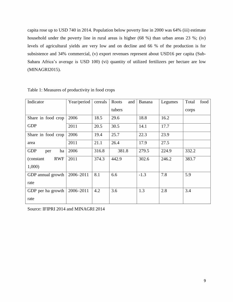
Table 1: Measures of productivity in food crops

Indicator Year/period cereals Roots and

tubers

Banana Legumes Total food

corps

Share in food crop

GDP

2006 18.5 29.6 18.8 16.2

2011 20.5 30.5 14.1 17.7

Share in food crop

area

2006 19.4 25.7 22.3 23.9

2011 21.1 26.4 17.9 27.5

GDP per ha

(constant RWF

1,000)

2006 316.8 381.8 279.5 224.9 332.2

2011 374.3 442.9 302.6 246.2 383.7

GDP annual growth

rate

2006–2011 8.1 6.6 -1.3 7.8 5.9

GDP per ha growth

rate

2006–2011 4.2 3.6 1.3 2.8 3.4

Source: IFIPRI 2014 and MINAGRI 2014

10

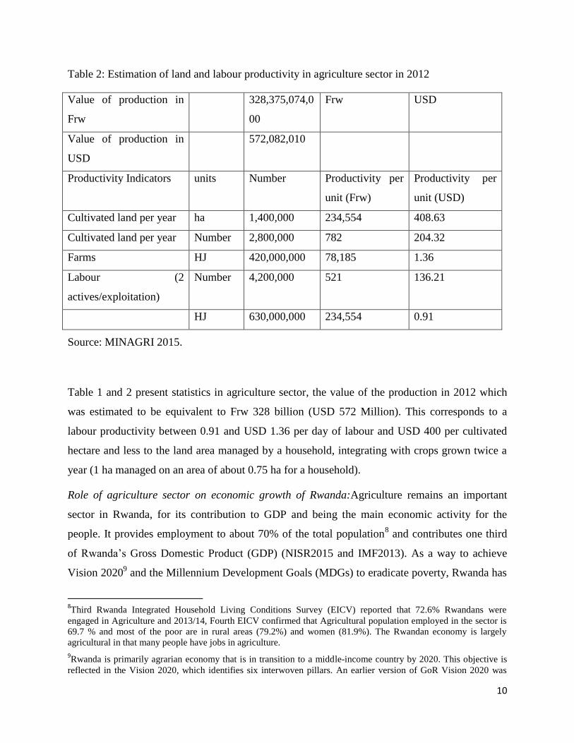
Table 2: Estimation of land and labour productivity in agriculture sector in 2012

Value of production in

Frw

328,375,074,0

00

Frw USD

Value of production in

USD

572,082,010

Productivity Indicators units Number Productivity per

unit (Frw)

Productivity per

unit (USD)

Cultivated land per year ha 1,400,000 234,554 408.63

Cultivated land per year Number 2,800,000 782 204.32

Farms HJ 420,000,000 78,185 1.36

Labour (2

actives/exploitation)

Number 4,200,000 521 136.21

HJ 630,000,000 234,554 0.91

Source: MINAGRI 2015.

Table 1 and 2 present statistics in agriculture sector, the value of the production in 2012 which

was estimated to be equivalent to Frw 328 billion (USD 572 Million). This corresponds to a

labour productivity between 0.91 and USD 1.36 per day of labour and USD 400 per cultivated

hectare and less to the land area managed by a household, integrating with crops grown twice a

year (1 ha managed on an area of about 0.75 ha for a household).

Role of agriculture sector on economic growth of Rwanda:Agriculture remains an important

sector in Rwanda, for its contribution to GDP and being the main economic activity for the

people. It provides employment to about 70% of the total population8 and contributes one third

of Rwanda’s Gross Domestic Product (GDP) (NISR2015 and IMF2013). As a way to achieve

Vision 20209 and the Millennium Development Goals (MDGs) to eradicate poverty, Rwanda has

8Third Rwanda Integrated Household Living Conditions Survey (EICV) reported that 72.6% Rwandans were

engaged in Agriculture and 2013/14, Fourth EICV confirmed that Agricultural population employed in the sector is

69.7 % and most of the poor are in rural areas (79.2%) and women (81.9%). The Rwandan economy is largely

agricultural in that many people have jobs in agriculture.

9Rwanda is primarily agrarian economy that is in transition to a middle-income country by 2020. This objective is

reflected in the Vision 2020, which identifies six interwoven pillars. An earlier version of GoR Vision 2020 was

11

improved the agricultural sector by sensitizing its citizens about farming techniques to increase

productivity. That will help do wipe out poverty and improve the standards of living for

everyone. Rwanda’s real economic growth for instance over the period 2008-2012 averaged

8.2% annually and thus translated into GDP per capita growth of 5.1% per year (MINECOFIN

2013).

In1996 it was estimated that 34 % of households were female-headed, out of which 21 % were

widows. The proportion of households headed by widows varies from Province to Province 13 %

in South province and 28 % in North province. Participation of the Rwandese women in

production and notably in agricultural production is something so common that any anomalies or

challenges in that field usually go unnoticed. A glimpse at their activities shows that: (i) rural

women work almost all the time without rest except for some hours of sleep and second (ii)

Women take part in all forms of activity whereas men do not do certain types of work reserved

for women by nature (breastfeeding, childcare) or by tradition (grinding on the traditional

grinding stone).Women play an important role in agricultural production activities.

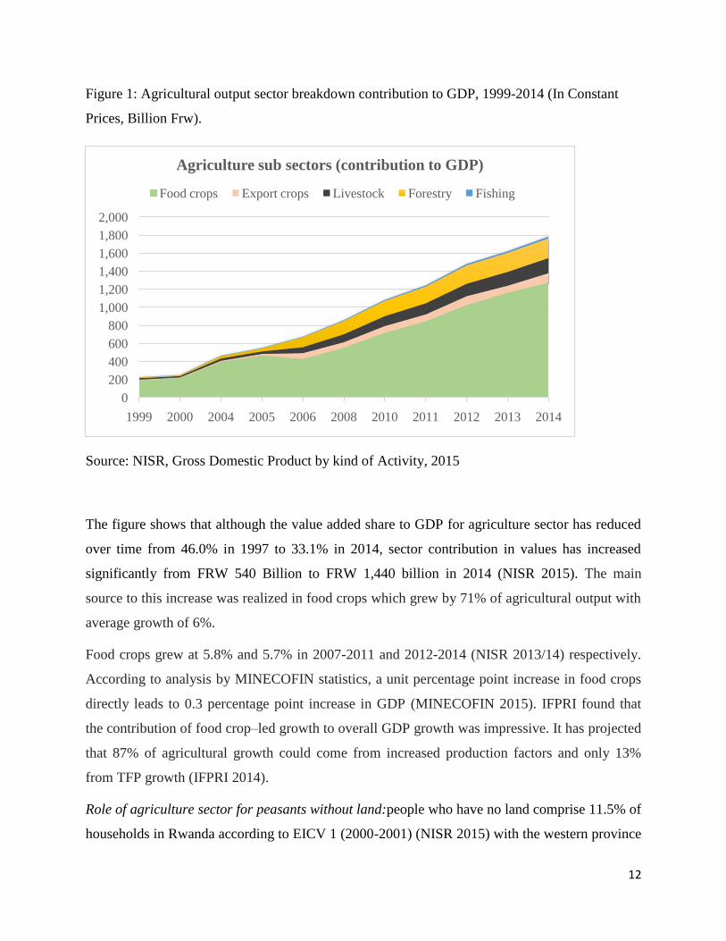
The economic activity was driven by a large increase in agricultural output, robust exports, and

strong domestic demand. The figure 1 below, shows trend broken-down of Agriculture

subsectors and evolution of their contribution to GDP from 1999 to 2014.

published in 2000 and has as objective: of transforming Rwanda from an agrarian subsistence economy into a

sophisticated knowledge based society.”

12

Figure 1: Agricultural output sector breakdown contribution to GDP, 1999-2014 (In Constant

Prices, Billion Frw).

Source: NISR, Gross Domestic Product by kind of Activity, 2015

The figure shows that although the value added share to GDP for agriculture sector has reduced

over time from 46.0% in 1997 to 33.1% in 2014, sector contribution in values has increased

significantly from FRW 540 Billion to FRW 1,440 billion in 2014 (NISR 2015). The main

source to this increase was realized in food crops which grew by 71% of agricultural output with

average growth of 6%.

Food crops grew at 5.8% and 5.7% in 2007-2011 and 2012-2014 (NISR 2013/14) respectively.

According to analysis by MINECOFIN statistics, a unit percentage point increase in food crops

directly leads to 0.3 percentage point increase in GDP (MINECOFIN 2015). IFPRI found that

the contribution of food crop–led growth to overall GDP growth was impressive. It has projected

that 87% of agricultural growth could come from increased production factors and only 13%

from TFP growth (IFPRI 2014).

Role of agriculture sector for peasants without land:people who have no land comprise 11.5% of

households in Rwanda according to EICV 1 (2000-2001) (NISR 2015) with the western province

0

200

400

600

800

1,000

1,200

1,400

1,600

1,800

2,000

1999 2000 2004 2005 2006 2008 2010 2011 2012 2013 2014

Agriculture sub sectors (contribution to GDP)

Food crops Export crops Livestock Forestry Fishing

13

(13%), North province (7.8%) and Eastern province (7.2%) on top of the list. Those households

without land and who have to rent it often get bad quality land. These families are often poor

with no means to acquire farm inputs, which would help to produce enough food for them. They

depend essentially on their productions for their livelihood and have no other source of income

apart from farming for others or renting land. Therefore any shock on their production (e.g.

climatic) throws them into a food insecurity situation.

Agriculture performance, especially during PSTA II was effective depending on the contribution

of the support sectors described below.

Governance and local development: decentralization process has transferred responsibility to

local governments and has created a situation of reducing the direct relationship between

MINAGRI and producers. Mechanisms and modalities adapted to the new situation has been

established so that requests from producers and grassroots receive the support contained in the

action plan of the ministry. The beneficiaries` needs collected in participatory workshops and

stored in a data base will serve as a mirror to all stakeholders to facilitate use of that information

in identification, funding and monitoring of agricultural micro projects initiated by grassroots

communities in a decentralized way.

Environment, water and land security: given that all environmental problems draw the interest of

all agriculture sub-sectors, attention to this issue will be integrated as crosscutting in all actions.

Anti-erosion fight, promotion of corridor cultivations, rational management of pastures and

intensive cattle raising systems, promotion of organic manure, biological methods of cultivation

and agro-forestry. (MINAGRI2014).

Commerce, industry and handicrafts: improvement and institutional capacity building will be

achieved through revision of the legal and regulatory framework. The latter must first create

conditions for food products safety. A study is to be conducted to establish an agency or another

institution in charge of food security and food safety standards. Such a structure should be

responsible for the coordination of activities, setting and controlling standards in matters of

national food safety, certification of food industries, programs of education on good cultivation

practices, danger control for food, implementing activities related to food products like the

National Bureau of Standards, reinforce national capacity namely of the National Office of

Standardization, develop national laboratories to carry out specific tasks. Promotion of agro


14

business is seeking improvement of added value of specific networks in order to serve internal

and external markets. Quality starts with production; good farming practices should be

introduced during production to avoid taking late corrective measures, after having suffered

losses. (MINAGRI 2014).

These considerations, indicate that the sector of commerce, industry and handicrafts is expected

to play a key role to foster the implementation of PSTA. Further to what is indicated, the

following complementary actions are expected: 1) promoting services for access to information,

access to training and local, regional and international markets; 2). develop, though appropriate

institutions, new transformation technologies, communication and marketing techniques, 3) set

international standards in matters of food safety and food hygiene, 4) foster networks and

associations of agribusiness with other regional and international organizations, 5) promote

initiatives and activities for the development of handicrafts and industry. (MINAGRI2014).

Infrastructure of transport and communication (ICT): cooperation is needed between

MININFRA in order: 1) to rehabilitate roads, 2) for promotion of transport of goods, easing

administrative constraints and diversification of routes and corridors for regional and

international trade, 3) dissemination of new information and communication technologies in

rural areas and to the professionals of the sector.

2.2. Review of literature on nexus between government spending and economic growth

Wagner Law (1835-1917) and Keynes 1936) saw that growth of public expenditure was a

consequence of economic growth in one way or another. Wagner introduced a model posterior

results) that public expenditures are endogenous to economic development.The basic Wagnerian

assumption is that public expenditure growths continuously associated with the continuing

growth in community output in developing countries. (Wagner 1883)

The Wagner’s work on impact of public expenditure on growth inspired a large number of

researchers in many ways. Recently a big number of researchers have been interested in studying

the law of increasing expansion of public expenditure, others the aspect of government spending

and government expenditure e.g. Barro (1990) and Yilgӧr, Ertuğrul and Celepcioğlu (2012).Also

investigating effects of those expenditures on economic growth (Hung Mo, 2007;Muhammad,



15

Xu and Karim, 2015; Al-Fawwaz, 2016; Danladi, Akomolafe, Olarinde and Anyadiegwu, 2015;

Okafor and Eiya, 2011) and further studies on the government expenditures/budget allocations

on agriculture sector, economic growth as well as the role of agriculture to economic

development of economies, Kareem, Bakare et al. (2015), Kuznets (1961) and Lawal (2011) and

Johnston and Mellor (1961).

According to Danladi et al. (2015) government expenditures are classified into three main types

depending to their purposes. Government purchases of goods and services for current use, also

referred to as government consumption, capital investments (intended for future benefits) and

transfers payments (investments that are not directly purchases of goods and services).

From the literature by above researchers, there are relatively large variation in their empirical

findings on the magnitude of the impacts and to some extent on the direction of impacts, due to

methodologies and data that have been employed. Many of those literature are clear on the

expected impacts of different types of public investment programs in many sectors on economic

growth and the poverty reduction.

Literature revealed that investments in core public goods have high payoffs, in the form of

economic growth and reduced poverty (World Bank 2014)10

. Findings by Danladi, Akomolafe,

Olarinde and Anyadiegwu (2015) and Fan et al. (2000) support that raising of the government

expenditure contribute to resilience of different sectors of economy. Danladi et al. (2015) found a

significant positive relationship between both capital expenditure and recurrent expenditures on

economic growth. Furceri (2007) examined the relationship between public expenditure and

economic growth, using cross-country panel data from 1970 to 2000, he found that countries

with higher government expenditure business cycle volatility have lower growth. Mogues, Fan

and Benin (2015) found that with increasing attention to investment in agriculture, is seen as

essential for achieving development goals.These studies have recommended that the

governments should give priority to investments in areas such as the infrastructure investments

and research: rural roads, agriculture, R&D and education.

However, there are also researchers whose studies revealed contrasting situations about the effect

of government expenditure.Egbetunde and Fasanya (2013) findings shown that impact of public

10

Agriculture is a crucial sector for realizing the MDGs of gender equality and environmental sustainability.

According to World Bank, increased productivity and commercialization of the agricultural sector was also directly

responsible for 45% of the 12 point poverty reduction under EDPRS I (2008-2012).

16

spending on growth is negative except the recurrent expenditure. Yilgӧr, Ertuğrul and

Celepcioğlu (2012) observed, in contrast to current and transfer expenditure no causal

relationship between investment expenditures and economic growth. Landau (1986) through his

study on government expenditure in 96 Less Developed Countries and developed countries,

found a negative relationship between the government expenditure in GDP and the growth of per

capita GDP. They found a very weak impact of government capital expenditures on economic

growth.Okafor et al. (2011) identified determinants which hinders the government expenditure to

grow and effect negatively the economic growth such as inflation and budget deficits.

Unidirectional relationship between government expenditure and GDP was found by

Muhammadet al. (2015) and in their study on impacts of increase in public expenditure on

poverty in Rwanda, Mackinnon et al. (2003) indicated that there was a negative and significant

correlation between what was defined as productive government consumption expenditure and

real per capita GDP.

2.3. Literature on Public expenditure-agriculture and economic growth nexus

Roetter et al. (2007)highlighted three specific roles of agricultural in rural development

strategies: i) basis for changing livelihoods, ii) provider of high quality affordable food and iii)

provider of environmental services and Johnston and Mellor (1961) have listed five contribution

the agriculture to economic growth among others are i) increased transfer of labor resources, ii)

increased capital formation and iii) increased purchasing power. They emphasizedthat

agricultural development often stimulate growth that extends well beyond rural areas over the

past decades, higher incomes from agriculture and access to cheaper food.

World Bank (2014), IMF (2013), IFIPRI (2014), Fan et al. (2000) and de Janvry and Sadoulet

(2010) revealed that agriculture-led development is fundamental to reducing poverty, generating

economic growth, reducing the burden of food imports and facilitating an expansion of exports.

Accordingly, agriculture was deemed to be given a more prominent as part of the development

agenda. Also the AU/NEPAD (2003) argued that most countries achieve rapid economic growth

only when it is accompanied by growth in agriculture. According to IMF, agricultural growth has

strongly supported the country’s growth and led to successfulness of the national recovery

strategy in Rwanda.

17

Johnston and Mellor (1961) concluded that capital accumulation which plays the vital role. The

capital accumulation depends upon the creation of surplus, as in an industry, the surplus is

created through profits of the industrialists etc. In the same way, the economists are of the view

that the surplus can also be created through agriculture. Chang, Chen and Hsu (2006), Kuznets

(1961), Johnson (1960), and Todaro and Smith (2014) that the creation of agriculture surplus

becomes possible by: increasing agriculture production, utilizing the surplus labour in agri.

Sector, supply of employment to non-agricultural sectors, imposing tax on agriculture. Sector

and keeping terms of trade against agriculture sector. Also the contribution of food crops studied

by IFPRI, in its results shown that are important to total agricultural and overall economy due to

its linkages effects to the rest of economy.

Mellor (1986),Chang et al. (2006), and Ademola et al. (2013) in their studies found that

agricultural sector has a significant role to encourage economic growth (in other words, it is a

variable) when examining the impact of economic growth. Oyakhilomenetal. (2013), Ebere et al.

(2012) and Chand et al. (2004) examined the government allocation to the agriculture sector and

economic growth in countries like Nigeria and Pakistan. From an econometric perspective, the

results of their analysis shown that the relationship between agricultural budgetary allocation and

economic growth is positive, however the sector still encountersproblems of inadequate

financing, poor infrastructures, farm fragmentation(Sandford1984).

Kareem, et al. (2015) and Ademola et al. (2013) found that government expenditures in

agricultural sector have significant impact on economic growth. While Ele et al. (2014), Benin et

al. (2009) and Iganiga et al. (2011) studying on impact of agricultural types of expenditure on

agricultural output growth in Nigeria and Ghana, found that government expenditures in

agricultural sector have significant positive impact on agricultural productivity, which led them

to conclude that if agriculture is properly funded it could bring about sustainable economic

growth.

Nevertheless in contrast to these above, Kumar, Kamble and Chaudhary (2014) andLooney

(1994) in his study found that deficiencies in several types of infrastructure psychical or soft for

agriculture i.e. irrigation, mechanization, cropping, public finance, investment in R&D among

others, may lead to moderate constraint on agricultural productivity.Johnson (1960), identified

problem of subsistence farming and Lawal (2011), IFPRI (2014), Sandford (1984) and Mogues,

18

Fan and Benin (2015), that government are inconsistent in financing it which justify

insignificance of contribution of thesector to the economic growth. Dholakia (2007) when he was

comparing contribution of various sectors in the Gujarat state, concluded that agriculture and

fishing among other areas were the weaker sectors in Gujarat economy due to inefficiencies in

implementing the policies of those sectors.

Mogues et al. (2015) revealed that in developing economies, agriculture sector was somehow

challenged by government policies and development paradigms towards the 1960s to the early

2000s. That was seen in declining or inappropriate public investments in agriculture. In addition,

(Kumar et al., 2014) and Fan et al. (2000) alsoinadequacy in use of fertilizers, public finance,

and small-landholding, cropping intensity, agricultural research and education, among others

factors for causing conditional convergence. Fan et al. (2000) indicated serious under-investment

in research on agricultural productivity, as evidenced by very high cost rates of return on

government investments11

.Inexistence of good accessible road networks; no accessible markets;

no power generations, no incentives, rather burdensome taxation on the side of the public finance

(World Bank 2007), limited provision of fertilizers, insecticides and pesticides; no provision of

irrigational facilities, better tools, and implements (tractors, etc. ); there was no means of

communication and transportations.

In their study on four countries, England, USA, South Korea and China, by Tsakok and Gardner

(2007) found little well-identified evidence on causal relationship between agriculture

developmental investments and economic growth. They controverted views that agriculture

development is necessary for overall economic transformation of economies, and revealed that

adverse supply shocks in agriculture sector could influence adversely the economy.Whereas

Kuznets (1961) expressed complexity of isolating the role of each of economic sector, including

agriculture to aspect of growth due to interdependence of the sectors. Chand and Kumar (2004),

observed an asymmetry in the effect of public investment on private investment by confirming

that increase in public investment induces a rise in private investment, whereas a decline has

adverse impact on the latter.

11

See IFPRI (2012) budgetary expenditures lead to capital formation in the agricultural sector. Capital formation

included physical and human capital.

http://www.agbioforum.org/v13n4/v13n4a03-ivanic.htm#R1

http://www.agbioforum.org/v13n4/v13n4a03-ivanic.htm#R1

19

Challenges limiting potential of agricultural productivity and growth and GDP growth has

merely attributed to reduced expansion of output in Agriculture being constrained by several

factors. Kumar et al. (2014) and AU/NEPAD (2003) viewed those limitations to agriculture

leading to low productivity. For the latter low productivity in agriculture is the result of low

investment in all the factors that contribute to agricultural productivity12

whereas for Kumar, it is

the nature which put limits on agricultural potentials. Therefore required that the profitability of

agricultural investments should be increased and made more attractive. Mogues et al. (2015) in

their study focusing on policy environment of greater attention needed for agriculture

investment, identified gaps in relation to that effect of government expenditure at different levels

of financing and effectiveness of investments were not receiving much attention.A general

summary of the literature on government expenditure and economic growth nexus and effect of

the government expenditure on agriculture is presented in Appendix A.

In addition, it was found by many scholars that agricultural growth has special powers in

reducing poverty across all country types. Cross-country estimates show that GDP growth

originating in agriculture is at least twice as effective in reducing poverty13

as GDP growth

originating outside agriculture. Similar importance have been highlighted by Thirtle et al. (2003)

and IFPRI (2014) whorevealed that agricultural growth brought by agricultural technology can

help to reduce poverty through lowering food prices, etc. . For Thirtle et al. (2003), every 1%

increase in yield brought about by investments in agricultural R&D, 2 million Africans can be

lifted out of poverty.

Although the rates of poverty14

reduction have been modest, in Rwanda between 2000 and

2007and have been not so fast enough to meet the global MDG targets, whereby the total number

of poor people was up to five million and over 90% of poor people were living in rural areas, the

pace accelerated both in rural and urban areas since the EDPRS 1 period (2008-2012) as result of

the government efforts seeking to transform the agriculture and the prioritization of the

12

Africa’s share of total world agricultural trade fell from 8 percent in 1965 to 3 percent in 1996. Low productivity is

the result of low investment in all the factors that contribute to agricultural productivity and effective use of

available resources. To correct the problem will require Africa to significantly increase investment in agriculture.

This in turn requires that the profitability of agricultural investments be increased and so made more attractive. 13

According to the World Bank increased productivity and commercialization of the agricultural sector was also

directly responsible for 45% of the 12 point poverty reduction under EDPRS I, 2008-2012. 14

Poverty levels overtime are presented in table 8 of appendix B

20

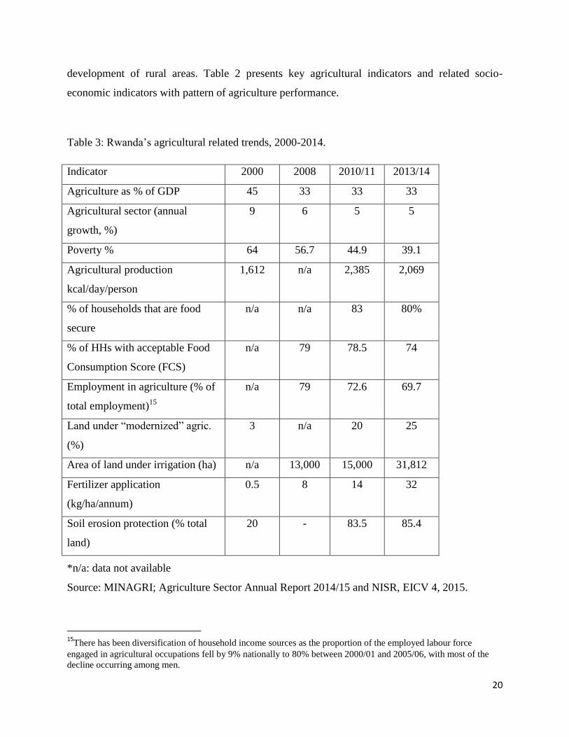
development of rural areas. Table 2 presents key agricultural indicators and related socio-

economic indicators with pattern of agriculture performance.

Table 3: Rwanda’s agricultural related trends, 2000-2014.

Indicator 2000 2008 2010/11 2013/14

Agriculture as % of GDP 45 33 33 33

Agricultural sector (annual

growth, %)

9 6 5 5

Poverty % 64 56.7 44.9 39.1

Agricultural production

kcal/day/person

1,612 n/a 2,385 2,069

% of households that are food

secure

n/a n/a 83 80%

% of HHs with acceptable Food

Consumption Score (FCS)

n/a 79 78.5 74

Employment in agriculture (% of

total employment)15

n/a 79 72.6 69.7

Land under “modernized” agric.

(%)

3 n/a 20 25

Area of land under irrigation (ha) n/a 13,000 15,000 31,812

Fertilizer application

(kg/ha/annum)

0.5 8 14 32

Soil erosion protection (% total

land)

20 - 83.5 85.4

*n/a: data not available

Source: MINAGRI; Agriculture Sector Annual Report 2014/15 and NISR, EICV 4, 2015.

15

There has been diversification of household income sources as the proportion of the employed labour force

engaged in agricultural occupations fell by 9% nationally to 80% between 2000/01 and 2005/06, with most of the

decline occurring among men.

21

Table 3 shows indicators on the performance of the sector. Poverty in Rwanda has been reducing

over time both in rural and urban areas. Population living under poverty line are now at 39.1%.

In 2014, studies by World Bank and IFPRI revealed that government expenditure on agriculture

did not only contributed toward the growth of agricultural output, but also indirectly to poverty

reduction. Over the last two decades, poverty had two peaks in 1980s and in the 1990s. The

proportion of poor households was 53 % in 1993. It sharply rose to 78% in 1994 and declined to

settle at 60 % in 2001 and 39.1% in 2013/14 (NISR 2015). Although, poverty was more rampant

in rural areas (68 %) than in towns (23 %) and further accompanied by other hardships such as

insufficient means of production or lack of access to land, as the average size of farming land

was 0.76 ha in 2000; (GoR 2015).

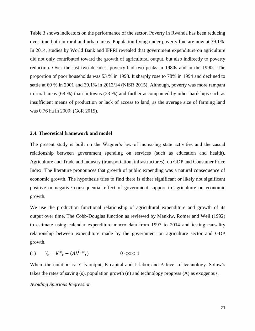
2.4. Theoretical framework and model

The present study is built on the Wagner’s law of increasing state activities and the casual

relationship between government spending on services (such as education and health),

Agriculture and Trade and industry (transportation, infrastructures), on GDP and Consumer Price

Index. The literature pronounces that growth of public expending was a natural consequence of

economic growth. The hypothesis tries to find there is either significant or likely not significant

positive or negative consequential effect of government support in agriculture on economic

growth.

We use the production functional relationship of agricultural expenditure and growth of its

output over time. The Cobb-Douglas function as reviewed by Mankiw, Romer and Weil (1992)

to estimate using calendar expenditure macro data from 1997 to 2014 and testing causality

relationship between expenditure made by the government on agriculture sector and GDP

growth.

(1) 𝑌𝑡 = 𝐾∝𝑡 + (𝐴𝐿

1−∝𝑡) 0 <∝< 1

Where the notation is: Y is output, K capital and L labor and A level of technology. Solow’s

takes the rates of saving (s), population growth (n) and technology progress (A) as exogenous.

Avoiding Spurious Regression


22

Spurious regression is misleading due to its ability to reflect false relationships between

variables; where aspurious regressionrefers to aregressionthat provides statistical evidence of a

linear relationship between independent non-stationary variables (Gujarati, 2003).

Before any empirical estimation is conducted it is necessary to conduct pre-unit root tests to

understand the underlying data generating process for application of suitable methodology.

Various parametric and non-parametric pre-testing methods are discussed in this subsection

before their pros and cons are highlighted.

Confirmatory Analysis

Results of the usual unit root tests can be confirmed using tests with stationarity as null

hypothesis.

These tests of confirmatory unit root testing with stationarity as null TEST 1 ( Usual test) can be

in the form as given by: 0H :tY non stationarity ( unit root) and 0H :

tY non stationarity ( unit

root),Maddala and Kim (1998).

These tests are conducted in either order and both reject the null hypothesis, then the presence of

unit roots cannot be confirmed. In his conclusion, he deduced that the 5% level of significance

gives better results than the 10% significance level. Joint non-rejections are far more common

than joint rejections.

However false confirmations are equally likely. If the true model is trend stationary, chances are

between 50-60% that confirmatory results are congruent with other pre-test results and half of

these are correct, when the true model is difference stationary, the proportion of confirmation is

60-65% of which about 82% are correct. Overall, many scholars are of the notion that unit root

tests are of some substance than using confirmatory analysis due to its defectiveness.

Model Diagnostic Inspection Analysis

After model specification, a battery of diagnostic instruments is applied to check if the model is

statistically adequate and the fitness of fit.

Most of them are more focused on diagnosing regression pathologies through regression

residuals. The presence of regression pathologies such as serial correlation, multi collinearity and

heteroscedasticity violates the classical assumptions of the Ordinary Least Squares, OLS and

23

hence invalidate statistical validity of parameter estimates. Application of co-integration test and

an establishment of linkage and direction of causality among the variables of interest was

followed to determine whether those are present and measure fitness of estimation using single

expanded equation (6).

2.5. Descriptive Analysis of the residual Analysis

The deficiency of a model can be detected by plotting the residuals. Outliers, in homogeneous

variances or structural breaks can be detected in the residual series. They are standardized before

plotting them to spot unusual residuals. To standardize them, their mean is calculated and

divided by their standard deviation to obtain the standardized residuals. If the residuals are

normally distributed with a mean of zero, roughly 95% of the standardized residuals should

deviate by a factor of 2 along the zero line. Autocorrelations and partial autocorrelations of the

residuals may be worth looking at because these quantities contain information on possible

remaining serial dependence in the residuals. The presence of serial autocorrelation in the

squared residuals is indicative of conditional heteroscedasticity in the model.

Examination of residuals through formal tests analysis

There are numerous diagnostic tests that can be applied to measure statistical adequacy of

models.

Serial correlation: the Breusch-Godfrey test (Verbeek 2000) is used extensively to detect for

higher order serial correlation in the residuals. There is a Lagrange Multiplier (LM) version as

well as the F-statistic version. Notably, the two versions are asymptotically equivalent. The LM

statistic for the null of interest can be obtained easily from the coefficient of determination R2 of

the auxiliary regression model. The null hypothesis of no serial correlation is rejected, both in the

LM and F-version testing approaches, if the probability value (p-value) is smaller than the level

of significance which can be at most 0.1 and at least 0.01 or 0.05.

Non-normality tests:the Jarque-Bera test of the normality of is used to detect violation of the

OLS assumption of normally distributed residuals in a model. This is against the assumption of

the classical regression model that residuals ought to be normally distributed with a mean of 0

and constant variance. The implication of violations of this assumption is that inferential

24

statistics of a model, such as the t-test and the F-test, are rendered invalid. The Jarque-Bera test is

based on the skewness and kurtosis of a distribution.

Heteroscedasticity:the statistical implication of heteroscedasticity is that the variance of residuals

is no longer constant. Although coefficients of estimated parameters are still unbiased and

consistent, their efficiency is lost. In fact the presence of heteroscedasticity causes the OLS

method to underestimate variances and standard errors, hence leading to overestimated and

misleading t-statistics and F-statistics (Asteriou and Hall 2007). The Breusch-Pagan and the

White tests are applied to check for heteroscedasticity in models (Gujarati 2003).

The LM and F versions are complementary and the null hypothesis of no heteroscedasticity

cannot be rejected if the p-value of the Breusch Pagan statistic is greater than the specified levels

of significance.

Autocorrelation LM test:autocorrelation can be defined as relation between members of a series

of observations ordered in time. It arises in cases where the data have a time dimension and

where two or more consecutive error terms are related. In this case, the error term is subject to

autocorrelation or serial correlation. It arises as a result of either excluded variables or the use of

incorrect functional form. The consequences of autocorrelation are that the OLS remains

unbiased, but becomes inefficient and its standardized errors are estimated in the wrong way

Gujarati (2003) and Verbeek (2000).

Residual normality test: the assumptions of the Classical Linear Regression Model (CLRM)

require that the residuals are normally distributed with zero mean and a constant variance and

violation of this restriction will result in t-and F-statistics being not valid. One way of detecting

misspecification problems is through observing the regression residuals. Usually the normality

test checks for skewness (third moment) and excess kurtosis. Jarque-Bera normality test

compares the third and fourth moments of the residuals to those from the normal distribution

under the null hypothesis that residuals are normally distributed.

Stability Analysis:It is tradition in modern empirical analysis to check for model stability over

time. As such parameter instability and structural change are inspected if there is a reason to

suspect structural breaks in the underlying data generating process. To this the CUSUM tests:also

the cumulative sum of recursive residuals (CUSUM) tests are to be applied. The CUSUM and

CUSUMQ are quite general tests of structural change in that they do not require prior

25

determination of where the structural break takes place. To check for impacts from suspected

simultaneous or synchronous shifts in parameters of the model, the CUSUM-of-squares

(CUSUM-SQ) plots are observed based on the formula below may be more informative.The null

hypothesis of structural stability is rejected if the plots cross the critical lines at 5% significance

level.

26

CHAPTER THREE: METHODOLOGY

3.1. Data

This section describes the methodology of the study and the data used. The research

methodology is the process used to collect data and other types of information for use in making

business decisions. Examples of this type of methodology include documentation surveys, and

research of publications. This part is about the overall approach to the research process, from the

rationale underpinning of the study to the collection and analysis of the data.

The study collected secondary data on macroeconomic variables for the period 1997-2014. In the

due course the researcher collected relevant data needed to test the research hypotheses. In this

study the researcher has adopted a case study approach, whereby Rwandan economy was

particularly chosen. A case study is an intensive description, analysis and interpretation of

economic correlation results between variables16

of Gross Domestic Product; Government

Expenditure on Agriculture; Agriculture Value Added; Purchases of Goods and Services; Gross

savings and Wages and Salaries in Rwanda during the period of the study based on information

obtained from the sources.

Data for these variables were presented in billion francs values (in Local Currency Unit,

LCU)17

at current prices on annual basis, however for the purpose of our analysis variables were

first transformed into logarithm to avoid problem of different time intervals between

observations.

The data were collected by using the secondary data in the study; the primary data has been

collectedby National Institute of Statistic of Rwanda (NISR), then the researcher has collected

the data of from MINECOFIN.Secondary sources of data for this study will include

macroeconomic statements, financial reports, government publications, library books and

internet sources.

16

Selected data are drawn are for macroeconomic indicators drawn from official reports by MINECOFIN retrieved

http://www.minecofin.gov.rw-MINECOFIN,MacroFramework_Public_Dataset-June_2015. These were

complemented by NISR publications and those downloaded from World Development Indicators Database (World

Bank, WID 2016). For example, data on GDP for 2 years before 1999 were not available from MINECOFIN and

NISR, but found on World Bank. Note. Data are presented in table 7 in appendix. 17

All variables were collected in Billions Franc, which is the LCU for Rwanda.

http://www.minecofin.gov.rw-minecofin,macroframework_public_dataset-june_2015./

27

Definitions of variables and parameter values inthe model: the variable to be explained in this

study is the gross domestic product (GDP which was defined in its value terms, In billion francs

(FRW). The GDP which was referred in the model as LGDP, according to NISR defines the sum

of gross value added by all resident producers in the economy measured as the difference

between production and intermediate consumption plus any product taxes and minus any

subsidies not included in the value of the products. Whereas the independent variable of our

interest was GEA: government expenditure on agriculture was taken in billion Frw as reported in

budget execution reports by MINECOFIN and MINAGRI.

AGVA: Agriculture value added (in Billion Frw of GDP), Forestry & Fishing, PGS: purchases of

goods and services as reported by MINECOFIN as component of the government expenditure,

WS: Government expenditure on Wages and Salaries in billion franc and GS: Gross savings

The expected signs (effect) of the explanatory variables on GDP consistent with the theories

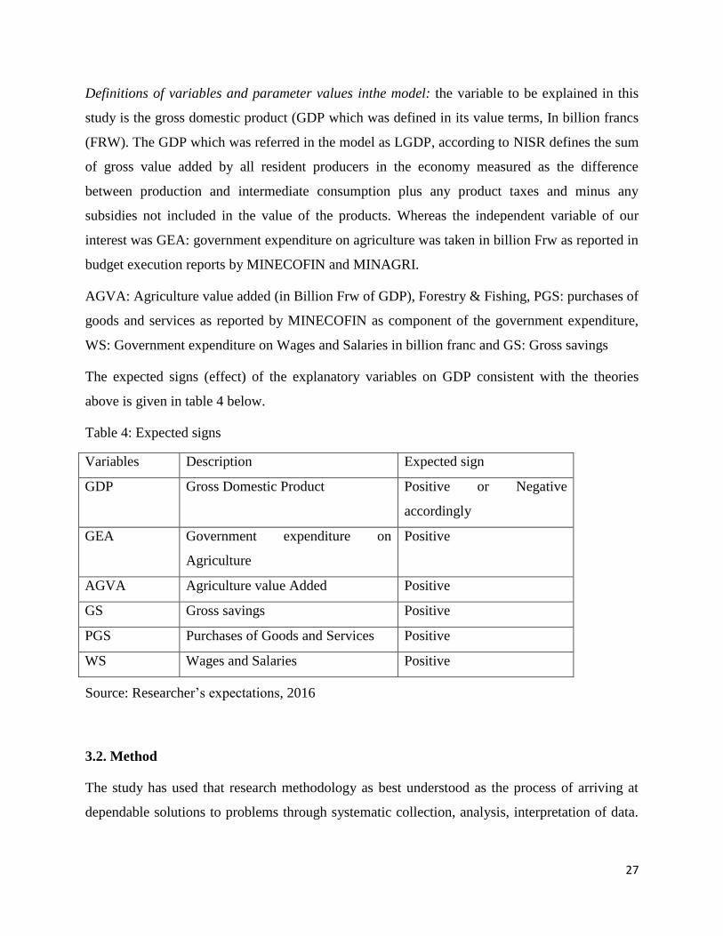
above is given in table 4 below.

Table 4: Expected signs

Variables Description Expected sign

GDP Gross Domestic Product Positive or Negative

accordingly

GEA Government expenditure on

Agriculture

Positive

AGVA Agriculture value Added Positive

GS Gross savings Positive

PGS Purchases of Goods and Services Positive

WS Wages and Salaries Positive

Source: Researcher’s expectations, 2016

3.2. Method

The study has used that research methodology as best understood as the process of arriving at

dependable solutions to problems through systematic collection, analysis, interpretation of data.

28

It is important to decide on the sources of data that would give most appropriate responses to the

questions and which methods and tools most appropriate to collect the relevant data.

The researcher has used quantitative as an approach that believes in quantifying responses in

different levels, it uses mathematical conclusions such as mean, percentages, standard deviation

etc. To show the degree of correlation of responses from different respondents, in this research

data was analysed through the sample tabulation of the targeted population and percentages was

calculated to describe the degree or level of correlation of the results collected from different

respondents. Measurement of the GDP and the relationship with the government spending on

agriculture used empirical analysis and model variable estimation referring to panel data. Panel

data due to the measure of time and place variations of growth as well as comparing trends and

performances across variables into considerations.

Macroeconomic research sample data:a sample was taken by the researcher as the process of

selecting people to be included in the research study. The immediate purpose of a sample is to

increase the ability of generalizing the outcome of the population and to ensure that the

population includes all units of interest to the study. The sample must always be viewed as an

approximation of the whole rather than as a whole in itself. Because of availability of different

variables which are presented in an economy, the researcher has chosen to analyse with the

macroeconomic and the econometric interpretation about Gross Domestic Product; government

expenditure on agriculture; agriculture value added; purchases of Goods and Services; Gross

savings and Wages and salariesin Rwanda for the period of 1997 to 2014.

Documentary sources, observation, (library and internet search) were used by the researcher to

collect secondary data while primary data was obtained through structure and unstructured of

research guide of National Institute of Statistic of Rwanda (NISR).Documentation have been

used by which contain the information about a phenomenon that researchers wish to study. In

this study the documents that will be targeted are number of documents available in the library,

on the internet web and the annual reports of the MINECOFIN, were consulted for the purpose

of obtaining secondary information relevant to the subject matter.

Key informant interviews: Key informant interviews are qualitative in-depth interviews with

people who know what is going on in a specific area of study. For the purpose of our study we

collected data from a wide range of people involved in agriculture including officials in

29

MINAGRI, NAEB, MINECOFIN, and NISR, experts in the sector and consultants who worked

in the field. Both telephone interviews and face to face interviews are applied here.

Econometrics modelling:the econometrics technique was used by the researcher for analysing

and interpreting the data from the results of all econometric tests which are presented in model

specification, estimation and results, where the econometrics approach as technique is the

application of mathematics, statistical methods, to economic data and is described as the branch

of economics that aims to give empirical content to economic relations.

Literally, the word “economics” means “measurement in economy”. Econometrics is a branch of

economic sciences which provides the result of a certain outlook on the role of economics,

consists of the application of mathematical statistics to economic data to lend empirical support

to the models constructed by mathematical economics and to obtain numerical results. The first

task of econometrics is to formulate an economic model.

3.3 The Model

As this chapter is based on the study of the effect of GEA on GDP in Rwanda, we can’t ignore

that the growth is explained by many variables, but here we are going to analyse this effect in

supply function by using GDP as endogenous variable and of GEA as exogenous variable.

As stated, our hypothesis is built on basic Wagnerian assumption that the government

expenditure growth is associated with the economic growth (Gemmell 1993:104). Wagner’s

suggestion had led to different literature including the study by Islam (1995) who examined

whether or not the results of the augmented Solow model obtained by MRW using cross-section

regressions change by using different techniques, namely panel data. Barro (1990), in turn, found

the government may affect the production function. For this study, since we are interested to

study the effect of government expenditure on agriculture to the GDP (as measure of economic

growth), and we refer our regression model on Wagner’s law.

http://en.wikipedia.org/wiki/Mathematics

http://en.wikipedia.org/wiki/Statistical_methods

http://en.wikipedia.org/wiki/Economics

http://en.wikipedia.org/wiki/Empirical

30

We begin with the Solow’s growth model18

that is reviewed by Mankiw, Romer and Weil (1992)

analyzed through the Cobb-Douglas production function and specify our model with variables of

interest in our study.

Further, Solow assumes factors governing evolutions in capital stock:

(2) 𝑘∗(𝑡) = 𝑠𝑓[(𝑘(𝑡)]− (𝑛 + 𝑔 + 𝛿)𝑘(𝑡)

Alternatively 𝑘∗𝑡 = [𝑠 (𝑛 + 𝑔 + 𝛿)]1 (1−∝)

Where n and g are exogenous parameters and where a dot over a variable denotes a derivative

with respect to time. 𝑠𝑓[(𝑘(𝑡), actual investment per unit of effective labor, Capital stock per

unit of effective labor, k, n+g, growth rate of effective labor, and 𝛿 is the capital depreciation

Since the central predictions of the Solow model concerned the impact of saving and population

on real income (this study derives its only model predicting the effect of government expenditure

on economic growth) and also depending on data under the study.

(3) 𝑌 = 𝛽𝑒𝜌𝑡𝐿𝛼𝐾1−𝛼

Where Y represents economic growth te is technical change which takes place at constant rate

in time t , L is labour force in the sector and K is public inputs in agriculture sector.

Our model is therefore formulated to measure the impact on growth considering different items

of government expenditures. A standard growth accounting model for this study, allows to

present different types of expenditures by government as determinants of growth, the model in

which variables are specified in linear log forms shown in equation (6).

(4) 𝑌𝑖𝑡 = 𝛽𝐺𝑖𝑡 + 𝛾𝑋𝑖𝑡 + 𝜇𝑖𝑡 + 𝑣𝑖𝑡 + 휀𝑖𝑡

Where itY - is the dependent variable (economic growth).

G is the government expenditure on agriculture and X is the vector of set of control variables,

identified as important variables for country expenditure-growth model, i indicates the

observations over time period, t from 1997 to 2014.

18

Equation (2) is the key equation of the Solow model. It states that the rate of change in the capital stock per unit of

effective labor is the difference between two terms.

31

is the parameter of interest capturing the effect of government expenditure on agriculture on

GDP.

it – Country fixed effects vector, it – Time fixed effects vector,

it – is the random error term

vector.

The error term is composed of two components휀𝑡 = 𝑣 + 𝜇, where v ~ N (0, 𝛿2) captures the

effects of the statistical noise and the second error component 𝜇≥ 0 is intended to capture the

effects of technical inefficiency. The it component represents things that cannot be controlled by

the farms like pests, insects and so on making the stochastic frontier allowing for variation across

farms. The i component represents the effects that can be controlled. Thus the producer

operates on or beneath stochastic production frontier according to whether i = 0 or i > 0. )

which is assumed to satisfy the usual properties of mean zero and constant variance and the

error term or disturbance term with normal distribution with mean zero and a constant variance

allowing to estimate the vector for the standard error; i =1, ..., nand t = 1, ..., T. Therefore, our

econometric model is expressed as the follows:

(5) 𝐺𝐷𝑃 =∝0+∝1 𝐺𝐸𝐴𝑖𝑡 +∝2 𝐴𝐺𝑉𝐴𝑖𝑡+∝3 𝑃𝐺𝑆𝑖𝑡 +∝4 𝐺𝑆𝑖𝑡 +∝5 𝑊𝑆𝑖𝑡 + 휀𝑖𝑡

In regards to test the hypothesis of relationship between GEA and GDP we apply a modified

version of the above specification (equation 2) which is often used by recent researchers and

referred to as advanced versions19

of the regression Model on Wagner’s Law. Variables in our

analysis were first transformed into logarithm to avoid problem of different time intervals

between observations:

(6) 𝐿𝐺𝐷𝑃 = 𝛽0 + 𝛽1𝐿𝐺𝐸𝐴𝑡 + 𝛽2𝐿𝐴𝐺𝑉𝐴𝑡 + 𝛽3𝐿𝑃𝐺𝑆𝑡 + 𝛽4𝐿𝐺𝑆𝑡 + 𝛽5𝐿𝑊𝑆𝑡 + 휀𝑡

Where, L is Natural Logarithm for variables, GDP is of Gross Domestic Product at period t,

GEA: Government Expenditure on Agriculture at period, AGVA: Agriculture value added, PGS:

Purchases of goods and services at period t, GS: Gross savings, WS: government expenditure on

wages and salaries, : Error term, i and t variable observations and time period from 1997 to

2014.

19

Literature detail six versions of the regression model on Wagner’s law.

32

𝛽0: is Intercept and 𝛽1,𝛽2,𝛽3,𝛽4,𝛽5 are Parameters of model. The null hypothesis of simple

linear specification is obtained: 𝐻0:𝛽1,𝛽2,𝛽3,𝛽4,𝛽5 = 0

Test of data

In order to measure all economic relationship between the presented variables of a model, the

researcher has to use time panels require the econometric tests. The theory of agricultural

growth, considered as an engine for overall growth for developing countries, has dominated

growth literature over the past half century. After demonstrating the expected signs in the

following section, the following point emphasizes those tests in order to get econometric results

which allow the researcher to make economic discussions, analysis and interpretations.

Using Ordinary Least Squares one calculates the restricted residual sum of squares ESSR

associated with model. Where휀𝑡 = 𝑣 + 𝜇𝑡 ; ν is the two-sided noise component, and μ is the

technical inefficiency component. The second method to apply is the GMM, to the regression

equation (1) discussed.

𝛽1,𝛽2,𝛽3,𝛽4,𝛽5 > 0: this means that the explanatory variables such as GEA, PGS, GS, AGVA,

WS are positively related to GDP, that is to say that when there is an increase of those

explanatory variables, we experience an increase in overall GDP.

𝛽1,𝛽2,𝛽3,𝛽4,𝛽5 < 0: this means that the explanatory variables GEA, PGS, GS, AGVA, WS are

negative related to GDP, that is to say that when there is a decrease of those explanatory

variables, we experience a decrease in overall GDP.

The study of the effect of GEA on GDP in Rwandacan’t ignore that the growth is explained by

many variables, but here we are going to analyse this effect in supply function by using GDP as

endogenous variable and GEA as exogenous variable. With adjustments incorporated into the

model in (4), it can therefore be specified in the form expressed decomposition of GDP growth

linked to variables of interest which was formulated in the following relation:

(7) 𝐺𝐷𝑃 = 𝑓(𝐺𝐸𝐴,𝐴𝐺𝑉𝐴,𝑃𝐺𝑆,𝐺𝑆,𝑊𝑆)

33

Equation (7) models the selected determinants of economic growth (GDP). These are

government expenditure on agriculture, Agricultural output, the purchase of good and services,

expenditure on wages and salaries and the gross savings.

In regards to test the hypothesis of relationship between GEA and GDP we apply a modified

version of the above specification (equation 4) which is often used by recent researchers and

referred to as advanced versions of the regression Model on Wagner’s Law. Therefore under this

study, the effect of GEA on economic growth which is measured as GDP, is estimated with help

of statistical software (EViews 7) with OLS equation expanded as follows.

(8) 𝐿𝐺𝐷𝑃 = 𝛽0 + 𝛽1𝐿𝐺𝐸𝐴𝑖𝑡 + 𝛽2𝐿𝐴𝐺𝑉𝐴𝑖𝑡 + 𝛽3𝐿𝑃𝐺𝑆𝑖𝑡 + 𝛽4𝐿𝐺𝑆𝑖𝑡 + 𝛽5𝐿𝑊𝑆𝑖𝑡 + 휀𝑖𝑡

Where, tLGDP : Logarithm of Gross Domestic Product in period t,

tLGEA : Logarithm of

Government Expenditure on Agriculture in period t, tLAGVA : Logarithm Agriculture Value

Added in period t, tLPGS : Logarithm Purchases of Goods and Services in period t,

tLGS : Logarithm Gross savings in period t; tLWS : Logarithm Wages and Salaries in period t, and

t : Error term in period t, Number of observations and t time periods from 1997 to 2014. 0 : is

Intercept and𝛽1,𝛽2,𝛽3,𝛽4,𝛽5 > 0: parameters of model.

Equation (6), is adopted because data are specific over period 1997 to 2014 and many are often

reported as subsets of the GDP. Thus, to examine effect of government expenditure to national

output. Also given that literature was interested to relationship between the economic growth and

the share of government expenditure had to influence its movement. The model assume that

government expenditure on agriculture sector increases the production of food, expansion of

export of cash crops as well as catalyze the manufacturing by agro-industries, increases farmers

savings and the purchase of goods and services such as machinery. Also according to Barro

(1990) and Kuzinets (1961), taken variables such as the size government expenditure, wages and

savings form determinants of Growth (GDP).

34

CHAPTER FOUR: DATA ANALYSIS, PRESENTATION AND INTERPRETATIONS

In this section, the researcher used to apply the econometric method in order to verify the

hypotheses of the study. To reach on goal, the researcher has developed different points like:

introduction to econometrics, specification of the model, expected signs, data processing, model

estimation and diagnostic tests by using the data of Rwandan economy from 1997 to 2014.

4.1. Estimation and testing the results

To estimate the parameters, we applied the panel data method and different types of panel

analytic models; which fit our model. Estimation techniques referred to are: OLS, Two stage

Least Squares (2SLS) and GMM. Followed steps are:

Data transformation or first-stage estimation into natural logarithm forms

Estimation of the variables by using Ordinary Least Squares method

Two stage LS with constant instruments: 1997-2014

Estimation of the variables by using GMM method

And testing stability diagnosis.

Table 5 and 6 report findings of estimationusing EViews regression applying Ordinary Least

Squares and 2 Stage LS results. Additional information and the GMM method findings are

shown in Table 10 in appendixD.20

20

Zhang and Fan (2004) used a dynamic GMM approach to estimate the effectsof infrastructure on agricultural

productivity using the Indian district level.The general methods of moment (GMM) has been introduced to

reducethe potential endogeneity of many independent variables when panel data are available. There is an appendix

table with all results obtained using also GMM.

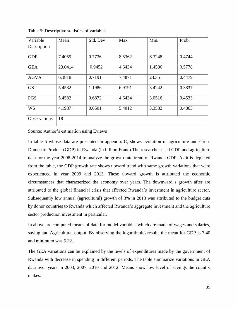
35

Table 5: Descriptive statistics of variables

Variable

Description

Mean Std. Dev Max Min. Prob.

GDP 7.4059 0.7736 8.5362 6.3248 0.4744

GEA 23.0414 0.9452 4.6434 1.4586 0.5778

AGVA 6.3818 0.7191 7.4871 23.35 0.4479

GS 5.4582 1.1986 6.9191 3.4242 0.3837

PGS 5.4582 0.6872 4.6434 3.0516 0.4533

WS 4.1987 0.6501 5.4012 3.3582 0.4863

Observations 18

Source: Author’s estimation using Eviews

In table 5 whose data are presented in appendix C, shows evolution of agriculture and Gross

Domestic Product (GDP) in Rwanda (in billion Franc).The researcher used GDP and agriculture

data for the year 2008-2014 to analyze the growth rate trend of Rwanda GDP. As it is depicted

from the table, the GDP growth rate shows upward trend with same growth variations that were

experienced in year 2009 and 2013. These upward growth is attributed the economic

circumstances that characterized the economy over years. The downward s growth after are

attributed to the global financial crisis that affected Rwanda’s investment in agriculture sector.

Subsequently low annual (agricultural) growth of 3% in 2013 was attributed to the budget cuts

by donor countries to Rwanda which affected Rwanda’s aggregate investment and the agriculture

sector production investment in particular.

In above are computed means of data for model variables which are made of wages and salaries,

saving and Agricultural output. By observing the logarithmic\ results the mean for GDP is 7.40

and minimum was 6.32.

The GEA variations can be explained by the levels of expenditures made by the government of

Rwanda with decrease in spending in different periods. The table summarize variations in GEA

data over years in 2003, 2007, 2010 and 2012. Means show low level of savings the country

makes.

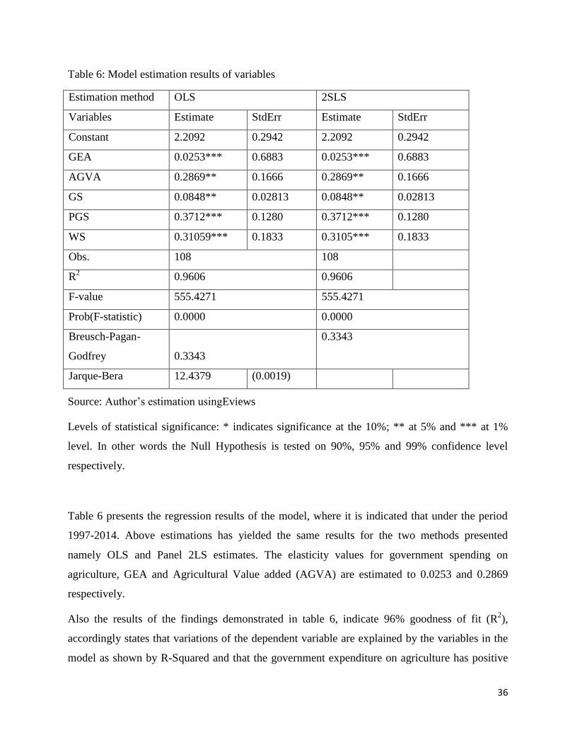
36

Table 6: Model estimation results of variables

Estimation method OLS 2SLS

Variables Estimate StdErr Estimate StdErr

Constant 2.2092 0.2942 2.2092 0.2942

GEA 0.0253*** 0.6883 0.0253*** 0.6883

AGVA 0.2869** 0.1666 0.2869** 0.1666

GS 0.0848** 0.02813 0.0848** 0.02813

PGS 0.3712*** 0.1280 0.3712*** 0.1280

WS 0.31059*** 0.1833 0.3105*** 0.1833

Obs. 108 108

R2 0.9606 0.9606

F-value 555.4271 555.4271

Prob(F-statistic) 0.0000 0.0000

Breusch-Pagan-

Godfrey 0.3343

0.3343

Jarque-Bera 12.4379 (0.0019)

Source: Author’s estimation usingEviews

Levels of statistical significance: * indicates significance at the 10%; ** at 5% and *** at 1%

level. In other words the Null Hypothesis is tested on 90%, 95% and 99% confidence level

respectively.

Table 6 presents the regression results of the model, where it is indicated that under the period

1997-2014. Above estimations has yielded the same results for the two methods presented

namely OLS and Panel 2LS estimates. The elasticity values for government spending on

agriculture, GEA and Agricultural Value added (AGVA) are estimated to 0.0253 and 0.2869

respectively.

Also the results of the findings demonstrated in table 6, indicate 96% goodness of fit (R2),

accordingly states that variations of the dependent variable are explained by the variables in the

model as shown by R-Squared and that the government expenditure on agriculture has positive

37

effect on GDP. The estimated results summarized in Table 6 show that an increase of one unit in

government expenditure on agriculture could have around 3% positive impact on economic

growth. Also the GMM results (reported in Table 10 in appendix D) indicate that coefficient for

GEA is significant at 1% level of significance, as 1 percent change in expenditure on agriculture

induce 8% increase of GDP. Therefore, effect of government expenditure on agriculture sector

on GDP in Rwanda cannot be ignored. From the results also, it is reflected that the growth is

explained positively by all variables selected for our model. However, here were interested to

analyse the effect of GEA in supply function (as defined in earlier part) by using GDP as

endogenous variable and of GEA as exogenous variable.

The results show that in long run, GEA explains GDP at 1% at level of significant as the

probability and T-statistic values are 0.7191 and 0.3682 respectively and the R squared=0.96.

Basing on economic theories, GEA does explain GDP in long run, 1 unit increase in government

expenditure on agriculture is reflected by 2.5% increase in GDP.

Alternatively other variables, selected to understand the role of government on growth such as

AGVA, GS, PGS, and WS and based on that performance of the model is good (R2

values for all

methods are greater to 80%) all have positive effect on Growth.The 96 goodness of fit (R2)

indicated that explanatory variables could explain the 96% variations in the dependent variable.

Accordingly Wages as current government expenditure that are wages and non-agricultural

employment are important sources of incomes to farmers and the incomes from wages them

contribute to the growth.

The results show that government spending on agriculture as well as other non- agriculture

spending for productivity-enhancing investments contribute positively to growth. However, for

GS and PGS, the impact has not been significant based on their probabilities.

Government spending on wages and Salaries contribute 0.31 at every 1 unit increase whereas

GEA effects 0.025 the GDP at each unit increase.

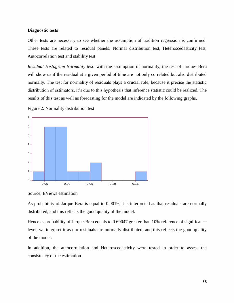
38

Diagnostic tests

Other tests are necessary to see whether the assumption of tradition regression is confirmed.

These tests are related to residual panels: Normal distribution test, Heteroscedasticity test,

Autocorrelation test and stability test

Residual Histogram Normality test: with the assumption of normality, the test of Jarque- Bera

will show us if the residual at a given period of time are not only correlated but also distributed

normally. The test for normality of residuals plays a crucial role, because it precise the statistic

distribution of estimators. It’s due to this hypothesis that inference statistic could be realized. The

results of this test as well as forecasting for the model are indicated by the following graphs.

Figure 2: Normality distribution test

Source: EViews estimation

As probability of Jarque-Bera is equal to 0.0019, it is interpreted as that residuals are normally

distributed, and this reflects the good quality of the model.

Hence as probability of Jarque-Bera equals to 0.69047 greater than 10% reference of significance

level, we interpret it as our residuals are normally distributed, and this reflects the good quality

of the model.

In addition, the autocorrelation and Heteroscedasticity were tested in order to assess the

consistency of the estimation.

0

1

2

3

4

5

6

7

-0.05 0.00 0.05 0.10 0.15

Series: ResidualsSample 1997 2014Observations 18

Mean 9.88e-16Median -0.020407Maximum 0.150047Minimum -0.054165Std. Dev. 0.050748Skewness 1.676515Kurtosis 5.311076

Jarque-Bera 12.43791Probability 0.001991

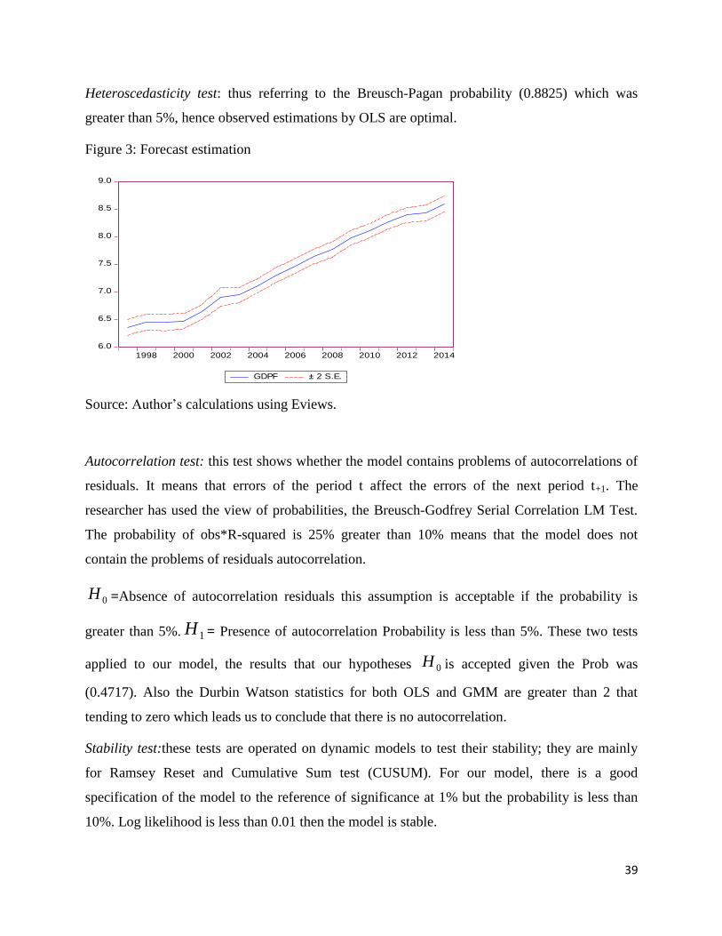
39

Heteroscedasticity test: thus referring to the Breusch-Pagan probability (0.8825) which was

greater than 5%, hence observed estimations by OLS are optimal.

Figure 3: Forecast estimation

Source: Author’s calculations using Eviews.

Autocorrelation test: this test shows whether the model contains problems of autocorrelations of

residuals. It means that errors of the period t affect the errors of the next period t+1. The

researcher has used the view of probabilities, the Breusch-Godfrey Serial Correlation LM Test.

The probability of obs*R-squared is 25% greater than 10% means that the model does not

contain the problems of residuals autocorrelation.

0H =Absence of autocorrelation residuals this assumption is acceptable if the probability is

greater than 5%. 1H = Presence of autocorrelation Probability is less than 5%. These two tests

applied to our model, the results that our hypotheses 0H is accepted given the Prob was

(0.4717). Also the Durbin Watson statistics for both OLS and GMM are greater than 2 that

tending to zero which leads us to conclude that there is no autocorrelation.

Stability test:these tests are operated on dynamic models to test their stability; they are mainly

for Ramsey Reset and Cumulative Sum test (CUSUM). For our model, there is a good

specification of the model to the reference of significance at 1% but the probability is less than

10%. Log likelihood is less than 0.01 then the model is stable.

6.0

6.5

7.0

7.5

8.0

8.5

9.0

1998 2000 2002 2004 2006 2008 2010 2012 2014

GDPF ± 2 S.E.

Forecast: GDPF

Actual: GDP

Forecast sample: 1997 2014

Included observations: 18

Root Mean Squared Error 0.049319

Mean Absolute Error 0.036868

Mean Abs. Percent Error 0.505719

Theil Inequality Coefficient 0.003313

Bias Proportion 0.000000

Variance Proportion 0.001078

Covariance Proportion 0.998922

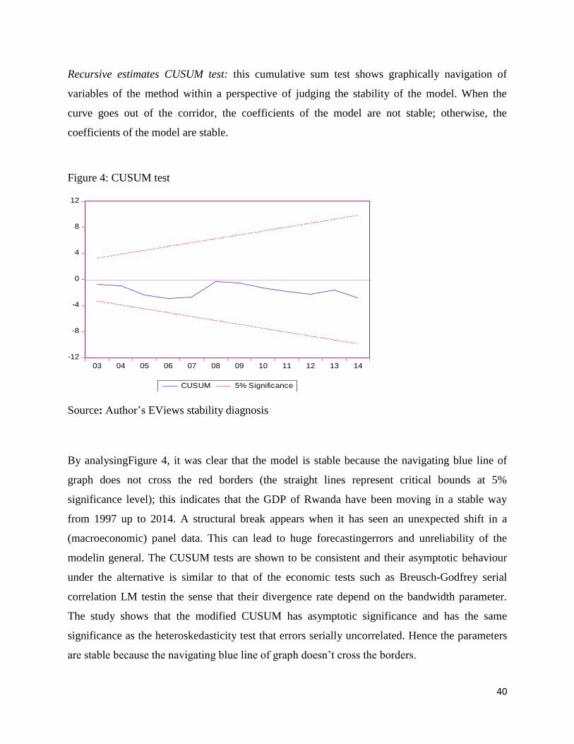
40

Recursive estimates CUSUM test: this cumulative sum test shows graphically navigation of

variables of the method within a perspective of judging the stability of the model. When the

curve goes out of the corridor, the coefficients of the model are not stable; otherwise, the

coefficients of the model are stable.

Figure 4: CUSUM test

-12

-8

-4

0

4

8

12

03 04 05 06 07 08 09 10 11 12 13 14

CUSUM 5% Significance

Source: Author’s EViews stability diagnosis

By analysingFigure 4, it was clear that the model is stable because the navigating blue line of

graph does not cross the red borders (the straight lines represent critical bounds at 5%

significance level); this indicates that the GDP of Rwanda have been moving in a stable way

from 1997 up to 2014. A structural break appears when it has seen an unexpected shift in a

(macroeconomic) panel data. This can lead to huge forecastingerrors and unreliability of the

modelin general. The CUSUM tests are shown to be consistent and their asymptotic behaviour

under the alternative is similar to that of the economic tests such as Breusch-Godfrey serial

correlation LM testin the sense that their divergence rate depend on the bandwidth parameter.

The study shows that the modified CUSUM has asymptotic significance and has the same

significance as the heteroskedasticity test that errors serially uncorrelated. Hence the parameters

are stable because the navigating blue line of graph doesn’t cross the borders.

https://en.wikipedia.org/wiki/Time_series

https://en.wikipedia.org/wiki/Forecasting

https://en.wikipedia.org/wiki/Economic_model

41

4.3. Empirical results and interpretations

The results are in consonant with discussions literature, Thirtle et al. (2003), Benin et al. (2009)

and Ebere and Osundina (2012), that public investment in agriculture has impact on agricultural

productivity and hence on economic growth. For instance, Ele et al. (2014), Shuaib et al. (2015)

and Ademola et al. (2013),found that government expenditure on agriculture and GDP are

positively related in Nigeria. Most specifically according to Oyakhilomen, Abdulsalam and

Rekwot (2013) when they analysed the link between agricultural budgetary allocations and

economic growth, arrive to conclude that there is positive relationship which was significant in

the long-run.

The impact of government support in agriculture and its impact on growth was studied by Lawal

(2011) in Nigeria, Looney (1994) and Johnston and Mellor (1961). All these found that

supporting agriculture was significantly related to the GDP growth.For Lawal, although

government expenditure on agriculture did not follow regular pattern, there was observed a direct

relationship between funding and the GDP growth. Looney and Mellor stated similar findings of

contribution of agriculture to GDP growth in that five classes as it: (a) meet a rapidly growing

demand for agricultural products associated with economic development (essentially a wage

goods argument); (b) increase foreign exchange earnings by expanding agricultural exports; (c)

supply Labour to the non-agricultural sector; (d) supply capital, particularly for its own growth,

for overheads and for secondary industry; and (e) serves as a market for industrial output.

The results presented are consistent with discussions that agricultural growth in Rwanda is

dependent to what government does, the public investments, much more on the production of

food crops, and the promotion of exports crops as well as seeking to reduce poverty.

(MINECOFIN, 2013; IMF, 2013; and Fan et al., 2000).

Given the model has other variables, selected to understand the role of government on growth

such as AGVA, GS, PGS, and WS and based on that performance of the model is good (R2

values for all methods are greater to 80%) all have positive effect on Growth, but for GS and

PGS, the impact is not significant.The estimated results on agricultural output, savings and

wages support different studies by previous researchers, e.g.on agricultural growth by (Ademola

et al., 2013; Iganiga and Unemhilin, 2011; IMF 2013 and Mogues, Fan and Benin, 2015).In that,

agricultural capital expenditure had a positive impact on agricultural output and economic

42

growth as well, (Ele, Okon, Ibok and Brown 2014, Iganiga and Unemhilin 2011 and Ebere and

Osundina 2012).

Wages as current government expenditure by Egbetunde and Fasanya (2013), Yilgӧr, Ertuğrul

and Celepcioğlu (2012), Danladi et al. (2015)and Fan et al. (2000), as for the latter, wages and

non-agricultural employment are important sources of incomes to farmers and the incomes from

them contribute to growth and poverty reduction. Whereas for savings and physical capital

expenditures by literature according Barro (1990) and Mankiw, Romer and Weil (1992). Higher

savings could lead to higher income, raise the total factor productivity, hence growth (Mankiw et

al.,1992). Also Mankiw et al. are conclusive on the importance of current expenditures (in

human capital) and capital (physical capital) as determinants of per capita growth.

43

CHAPTER FIVE: SUMMARY, CONCLUSION AND RECOMMENDATIONS

5.1. Summary of results and usefulness

Agriculture accounts one third of Rwanda’s economic activity and the sector has gained

government attention over the last two decades. Beyond of being among most populous country,

Rwanda accelerated growth of the economy by actively investing in Agriculture to ensure it

achieves food security and its economic recovery after 1994 genocide. Because of the great

importance of agriculture sector, it was deemed important to conduct this study with aim to

examine significance of impact of government expenditure on the sector toward boosting the

economic growth and the effects of these investments on the high growth progress realized by

since 2000s to 2014. Also effects of other variables of growth such as agriculture value added in

period; expenditure on purchase of goods and services in period; wages and Salaries and national

savings were estimated.

The findings indicated the extent to which support to agriculture has played in the sector’s

growth. The findings inform the government which component of expenditureshave been

significant in enhancing the performance of the GDP and encourage economic restructuring to

shift to growth oriented financing. Also enhance to stimulate and supplement the process of

agricultural productivity growth.This contributes to clarifying and correcting what has been for

long time prevailed as conventional wisdom regarding the support to agriculture and poverty

alleviation linkages. Also add to existing knowledge to assisting policy analysts and their

policymaker clientele in their considerations for related policies.

Findings are so important to the government to improve coordination of its programmes and

expenditures it makes, to improve the targeting of funds to the most productive areas and

encouraging activities that increase productivity. The results presented are consistent with the

idea that agricultural growth in Rwanda is dependent to the public investment of the government,

much more on the production of food crops, advancements that the government has been

implementing in agriculture regarding land consolidation, soil conservation and irrigation, etc.

Such findings may prove useful to policy analysts and planners concerned with development

agenda and design of agricultural policies and programs as well as resource mobilization.

44

However, there was an issue of data that limited the study to estimating agricultural growth

models in-depth and the importance of availing ready to use, consistent international and

disaggregated central and decentralized level data has been raised. Thus, if resolved that will

facilitate future researchers’ ability to analyse and explain with full evidence agricultural sector

the support and role of government to agriculture and toward growing economies of nations

around the world.

The study resorts to economic theory to recommend for increased expenditures in this sector

which is important pillar of the economy. Rationalization of the expenditure, streamlining of

roles and responsibilities for a clearer division of the budget across sectors and a more effective

means of targeting outcomes.

Rwanda could improve the effectiveness of investment especially in agricultural R&D and

should continue to do as these investment can have high payoffs in achieving multiple wins

increasing productivity and improving resilience and resource-use efficiency. However, climate

change reduced returns from investments and population which is high where majority of

farmers occupy less 0.5ha and recent studies shown that boosting agricultural growth through

induced innovations can exacerbate landlessness and inequality for the poorer rural inhabitants.

To reduce the large donor dependence in the agriculture sector and increase public financing

within the agriculture sector that empowers and benefit smallholders’ women farmers.

Fair sharing concept of public private partnership, government should widen incentives to the

private sector to increase mechanization with other-yield increasing types of inputs. Additional

relevant expenditure which contribute directly to increased agricultural development. These

include: applied agricultural research; multi-purpose development projects with agricultural

benefits; effective food and nutrition security interventions; and agricultural climate change

adaptations.

45

5.2. Summary and conclusion

As the aim of this study was to examine the effect of government support on agriculture to the

economic growth in Rwanda for the period of 1997-2014, using variable data in local currency

units (current prices) modelled after logs transformation. The analysis shown a general

significance of government expenditure to agricultural sector and significant impact on economic

growth.

Although, the performance of agricultural has been increasing, the share to national budget

fluctuated time to time due to changes in government fiscal policies and sometimes to

international factors or crisis. Agricultural support shown positive effect in accelerating the GDP.

The effect was explained by that the R squared scored 96%, and the sign for coefficient of

parameter (0.0253; OLS estimation) is positive, which means, a one increase in government

expenditure on agriculture is associated with a 2.5% increase in GDP. In summary, despite data

limitations to extend the period under the study, findings support the assumption that effect of

government expenditure on agriculture on GDP was significant over the period 1997 to 2014.

Rwanda has made progress in increasing the production form agriculture and since 1994,

initiatives for increasing public support in the agriculture sector and the upward trend in this

direction is required to continue. The faster rate of GDP growth realized in 2008 has fallen since

afterward, due falling agricultural growth which became unpredictable. The upward trend could

again happen if the country remains open to capturing investments in agriculture, R&D,

infrastructure and remain consistent in funding agriculture.

Recently, works to examine the size of the support of government, the levels and quality of

government expenditures in the agriculture sector in light of the commitment of the 10%

expenditure target and enhanced quality of government expenditure on agriculture (GEA) has

gained much attention.

5.3. Recommendations and suggestions for future data and researches

Although the study revealed the significant of government expenditure to stimulate the national

growth, that could not be probably unique to agriculture sector, we suggest areas of investigation

that could provide wide perspective about the role of government across other sectors to promote

economic growth. These are proposed to see the efficacy of public expenditure within sectors

46

like education, ICT and communication and infrastructure sectors (Energy and Transport) as well

as their role in fast growing the economy. These with regards to provide empirical evidence to

inform policies and programmes leading to successful implementation of the SDGs and Vision

2050 for which Rwanda has adopted to shape its long-term agendas to realize full economic

transformation and achieve free poverty.

Finally, limitations encountered that need to be addressed to allow better findings in the next,

e.g. limitations of data availability and their reliability. Along the study, data on expenditure in

agriculture, agriculture production were not enough disaggregated to agricultural zones nor at

district levels yet. It is also difficult to allow regional analysis due to that data on expenditure in

agriculture are not found to the World Bank source, but only found collected in local

documentations.

In many cases, data were not consistent and difficult to find for the very early years such as

before 1995 e.g. the necessary data on government expenditure on agriculture to include more

years for the study were not available. Also data on decentralized, detailed budget executions,

data of crop production structured by crops and by region though currently are being improved

by NISR through its agricultural surveys with help of UNDP, were not enough and not available

for lot of years for the period studied in order to be considered in the regression. The researcher

was forced to use national data when examining relationship between government expenditure in

agriculture and the economic impact on GDP growth.

The GoR should increase public spending on agriculture sector-which is important pillar

of the economy.

Rwanda should remain open regarding the capturing of investments in agriculture, R&D,

infrastructure.

Government should ensure consistency while financing the sector (due to that share of

spending fluctuated time to time)

Impact of spending in other sectors like education, ICT and Communication and

infrastructure sectors (Energy and Transport) should be examined too.

The financing for agricultural development through applied agricultural research, food

and nutrition security interventions and agricultural climate change adaptations.

47

REFERENCES

Ademola, S. I.; S.O Olaleye; A. E. Olusuyi and F. Edun (2013). Government Expenditure on

Agricultural Sector and Economic Growth in Nigeria (1981-2010). Journal of Humanities

and Social Science (IOSR-JHSS), 8(4): 62-67.

Al-Fawwaz, M. T. (2016). The Impact of Government Expenditures on Economic Growth in

Jordan (1980-2013). International Business Research; 9(1): 99-105.

Asteriou, D., and S. G. Hall (2007). Applied econometrics: A modern approach using EViews

and Microfit (Rev. ed.). Palgrave Macmillan. New York.

AU/NEPAD, (Africa Union/New Partnership for Africa Development) (2003). Comprehensive

Africa Agriculture Development Programme (CAADP).NEPAD, Midrand, 1-116.

Barro, J., R. (1990). Government Spending in a Simple Model of Endogenous Growth. Journal

of Political Economy, 98 (5): 103-125.

Benin, S.; T. Mogues, G. Cudjoe, and J. Randriamamonjy (2009). Expenditures and agricultural

productivity growth in Ghana. International Food Policy Research Institute, 1-32.

Chand, R. and P. Kumar (2004). Determinants of Capital Formation and Agriculture Growth:

Some new explorations. Economic and Political Weekly, 39(52): 5611-5616.

Chang, J., J.; B., L. Chen and M., Hsu (2006). Agricultural productivity and economic growth:

role of tax revenues and infrastructures. Southern Economic Journal, 72(4): 891-914.

Danladi J. D.; K., J. Akomolafe; O., S. Olarinde and N., L. Anyadiegwu (2015). Governement

expenditure and its implications for economic growth: Evidence from Nigeria. Journal of

Economics and Sustainable Development. 6(18):142-150.

de Janvry, A. and E. Sadoulet (2010). Agricultural growth and poverty reduction: Additional

Evidence. The World Bank Research Observer, 25(1):1-20.

Dholakia, H. R (2007). Sources of economic growth and acceleration in Gujarat. Economic and

Political Weekly, 42 (9):770-778.

Ebere, C. and K. C. Osundina (2012). Government Expenditure on Agriculture and Economic

Growth in Nigeria, International Journal of Science and Research (IJSR), 3(9): 188-193.

48

Egbetunde, T. and I. O. Fasanya (2013). Public Expenditure and Economic Growth in Nigeria:

Evidence from Auto-Regressive Distributed Lag Specification. Zagreb International Review

of Economics & Business, 16(1): 79-92.

Ele, I., E.; E. Okon; O. W. Ibok and I. N. Brown (2014). Analysis of agricultural public capital

expenditure and agricultural economic growth in Nigeria 1961-2010, American Journal of

Experimental Agriculture, 4(4): 443-456.

Fan, S., P. Hazell and S. Thorat (2000). Government spending, Growth and poverty in India,

American Journal of AgriculturalEconomics, 82(4): 1038-1051.

Furceri, D. (2007). Is Government Expenditure volatility harmful for growth? A cross-country

Analysis. Institute for fiscal studies, 28(1): 103-120.

Gemmell, N. (1993). The growth of the Public sector: theories and international evidence.

Victoria University of Wellington, New Zealand. 103-104.

Government of Rwanda (2015). Rwanda nutrition, Market and Gender analysis 2015: An

integrated approach towards alleviating malnutrition among vulnerable population in

Rwanda. International Center for Tropical Agriculture (CIAT): 33-224.

Gujarati, N., D. (2003). Basic econometrics, 4.ed. McGraw-Hill, New York.

IFPRI (Diao, X., G. Bahiigwa and A. Pradesha) (2014). The Role of Agriculture in the fast-

growing of Rwandan economy: Assessing Growth Alternatives. International Food policy

Research Institute (IFPRI), Discussion paper 1363, Washington, DC:

http://ebray.ifpri.org/cdm/ref/collection/p15738coll2/id/128243.

Iganiga, B., O. and D., O. Unemhilin (2011). The Impact of Federal Government Agricultural

Expenditure on Agricultural Output in Nigeria. Journal of Economics, 2(2): 81-88.

IMF (2013) World Economic and Financial surveys 2013: Regional Economic Outlook (REO):

Sub-Saharan Africa keeping the pace, IMF, 1-48.

Johnson, E., S. (1960). Potential Contribution of Agriculture to Economic Growth in Less-

Developed Countries. The Annals of the American Academy of Political and Social Science,

33(1): 52-57.

http://ebray.ifpri.org/cdm/ref/collection/p15738coll2/id/128243

49

Johnston, B., F. and J. W. Mellor (1961). The role of agriculture in economic development.

American Economic Review, 51(4): 566-593.

Kareem, R. O.; H. A. Bakare; G. R. Ademoyewa; S. E. Ologunla and A. R. Arije (2015). Nexus

between federal Government spending on Agriculture, agricultural output response and

economic Growth of Nigeria (1979-2013). American Journal of Business, Economics and

Management, 3(6):359-366.

Kelly, A. V., E. Mpyisi, A. Murekezi and D. Neven (2001). Fertilizer Consumption in Rwanda:

Past Trends, Future Potential, and Determinants. Paper presented in the Fertilizer Use and

Marketing Policy Workshop: 1-15.

Kumar, S.; A.; L., Kamble and K., R., Chaudhary (2014). Agricultural Growth and Economics

Convergence in Indian Agriculture. Indian Journal of agriculture Economics, 69(2): 211-

228.

Kuznets, S. (1961). The role of Agriculture in Economic development.International Journal of

Agrarian affairs, 3 (2), 56-75.

Landau,D. (1986). Government and Economic Growth in the Less Developed countries: An

Empirical Study for 1960-1980. Economic Development and Cultural Change, 35(1): 35-75.

Lawal, A., A. W. (2011). An analysis of government spending on agricultural sector and its

contribution to GDP in Nigeria. International Journal of Business and Social Science; 2(20):

244-250.

Looney, E., R. (1994). The impact of infrastructure on Pakistan’s Agricultural Sector. The

Journal of Developing Areas, 28(4): 469-486.

Mackinnon, J., A. Thomas, I. Hakizinka and L. Rugwabiza (2003).The impact of increases in

Public expenditure on poverty reduction in Rwanda, Oxford Policy Management for DFID:

1-34.

Maddala, S., G.and I. M. Kim (1998). Unit Roots, Cointegration and Structural Change.

Cambridge University Press, Cambridge.

Mankiw N. G.; D. Romer and D. N. Weil (1992). A contribution to the empirics of economic

growth. Quarterly Journal of Economics, 107(2): 407-437.

50

Mellor J. W (1973). Accelerated growth in agricultural production and the intersectoral transfer

of resources, Economic Development and Cultural Change, 22(1): 1-16

Ministry of Agriculture and Animal Resources (2006, 2007, 2008, 2009/10, 2010/11, 2011/12,

2012/13 and 2013/2014). Agricultural Sector Annual Reports, MINAGRI.

Ministry of Agriculture and Animal Resources (2009). Strategic Plan for the Transformation of

Agriculture in Rwanda phase II (PSTA II 2009-2012), MINAGRI, 1-128.

Mogues T., S. Fan and S. Benin (2015). Impact of public investments in and for Agriculture.

European Journal of Development Research, 27(3), 337–352.

Muhammad, F.; T. Xu and R. Karim (2015). Impact of government expenditure on economic

growth in Pakistan. International Journal of Academic Research in Business and Social

Sciences, 5(2):231-236.

National Institute of Statistics of Rwanda (2015). Fourth Rwanda Integrated Household Living

Conditions Survey (EICV 4, 2013/2014) Main indicators, NISR, 1-170.

National Institute of Statistics of Rwanda (NISR 2014). Fourth Population and Housing Census,

Rwanda 2012. 1-257.

Okafor, C. and O. Eiya (2011). Determinants of growth in government expenditure: an empirical

analysis of Nigeria. Research Journal of Business Management, 5(1): 44-50.

Oyakhilomen, O.; A., Z. Abdulsalam and G. Z. Rekwot (2013). Agricultural Budgetary

Allocations and Economic Growth in Nigeria: Implications for Agricultural Transformation

in Nigeria. The Journal of Sustainable Development, 10(1): 16-27.

Republic of Rwanda (2007 and 2013). Economic Development and Poverty Reduction Strategy,

EDPRS 1 (2008-2012) and EDPRS 2 (2013-2018), MINECOFIN.

Roetter, R. P.; H. van Keulen, M. Kuiper, J. Verhagen and H. H. van Laar (2007). Science for

agriculture and rural development in low-income countries. Springer, 3300 AA Dordrecht,

the Netherlands.

Sandford C.(1984). Economics of Public finance: an economic analysis of government

Expenditure and revenue in the United Kingdom. 3rd

Edition, Pergamon Press, Headington

Hill Hall, U.K.

51

Shuaib, I. M., F.E. Igbinosun and A. E. Ahmed (2015). Impact of government Agricultural

Expenditure on the growth of the Nigeria Economy. Asian Journal of Agricultural

Extension, Economics & Sociology, 6(1): 23-33.

Thirtle, C., L.,Lin and J. Piesse (2003). The impact of research led agricultural productivity

growth on poverty reduction in Africa, Asia and Latin America.World Development, 31(12):

1959-1975.

Todaro, M. and P., S. C. Smith. (2014). Economic Development in the World, 12th Edition,

England.Pearson Educations Limited, 437-458.

Tsakok, I. and B. Gardner (2007). Agriculture in Economic Development: Primary Engine of

Growth or Chicken and Egg? Journal of Agricultural Economics, 89(5): 1145-1151.

Verbeek, M. (2000). A Guide to Modern Econometrics.John Wiley & Sons, New York. 2000.

Wagner, A (1883), “Three extracts on public finance”, translated and reprinted in R.A.Masgrave

and A.T. Peacock (eds), classics in the theory of public finance, London: McMillan, 1958.

World Bank (2007) Fertilizer use in African agriculture: lessons learned and good practice

guidelines, WB Washington DC, Agricultural Policy Note 20433-RW.

World Bank (2014). Promoting Agricultural Growth in Rwanda: Recent Performance,

Challenges and Opportunities. WB Washington, DC, Rwanda Agricultural Policy Note

86399-RW.

World Bank (1998). Rebuilding an equitable society: Poverty and poverty reduction after

genocide, Macroeconomics, Rwanda Poverty Note., 17792-RW, Washington D.C

Yilgӧr, M.; C. Ertuğrul; and M. E., Celepcioğlu (2012).The effect of Public Expenditure on

economic growth: Turkey Example”. Investment Management and Financial Innovation,

9(2), 193-202.

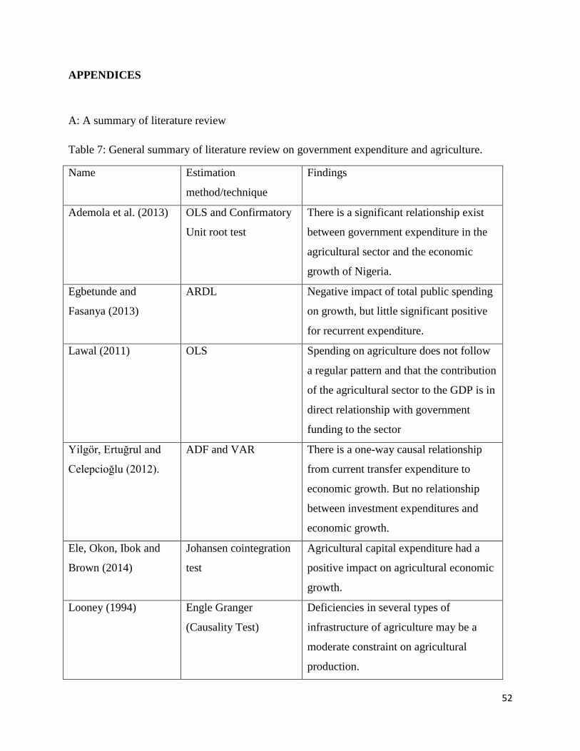
52

APPENDICES

A: A summary of literature review

Table 7: General summary of literature review on government expenditure and agriculture.

Name Estimation

method/technique

Findings

Ademola et al. (2013) OLS and Confirmatory

Unit root test

There is a significant relationship exist

between government expenditure in the

agricultural sector and the economic

growth of Nigeria.

Egbetunde and

Fasanya (2013)

ARDL Negative impact of total public spending

on growth, but little significant positive

for recurrent expenditure.

Lawal (2011) OLS

Spending on agriculture does not follow

a regular pattern and that the contribution

of the agricultural sector to the GDP is in

direct relationship with government

funding to the sector

Yilgӧr, Ertuğrul and

Celepcioğlu (2012).

ADF and VAR There is a one-way causal relationship

from current transfer expenditure to

economic growth. But no relationship

between investment expenditures and

economic growth.

Ele, Okon, Ibok and

Brown (2014)

Johansen cointegration

test

Agricultural capital expenditure had a

positive impact on agricultural economic

growth.

Looney (1994) Engle Granger

(Causality Test)

Deficiencies in several types of

infrastructure of agriculture may be a

moderate constraint on agricultural

production.

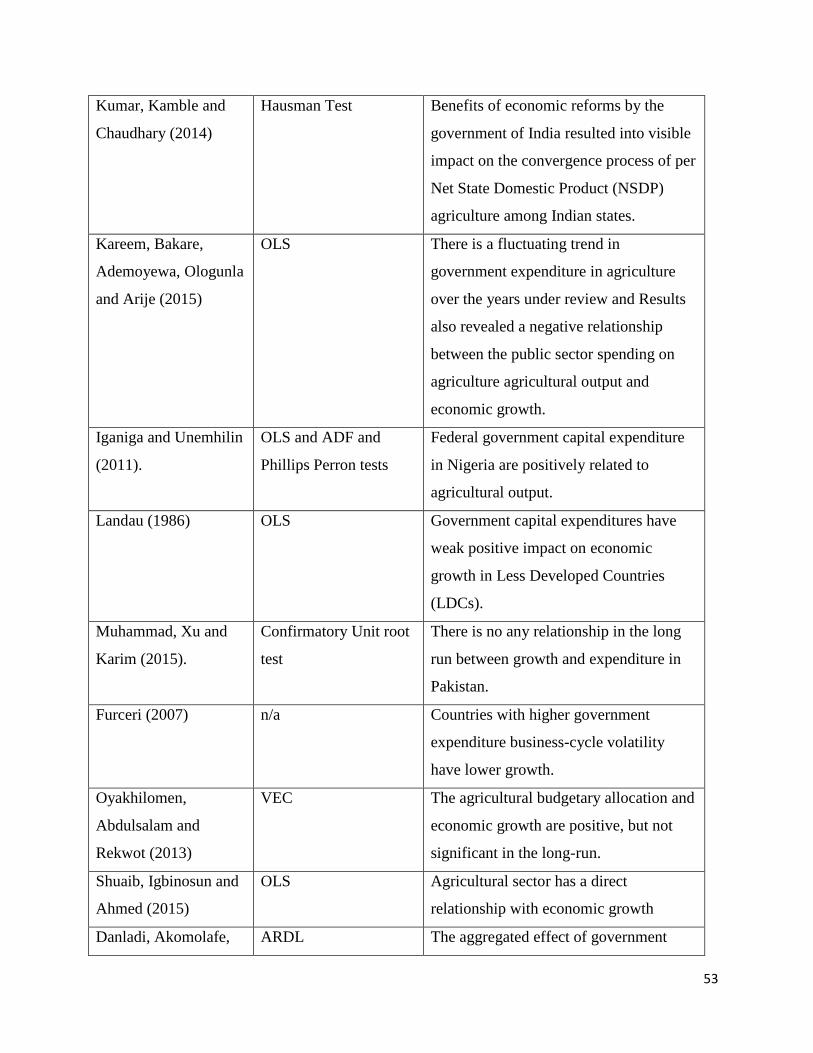
53

Kumar, Kamble and

Chaudhary (2014)

Hausman Test Benefits of economic reforms by the

government of India resulted into visible

impact on the convergence process of per

Net State Domestic Product (NSDP)

agriculture among Indian states.

Kareem, Bakare,

Ademoyewa, Ologunla

and Arije (2015)

OLS

There is a fluctuating trend in

government expenditure in agriculture

over the years under review and Results

also revealed a negative relationship

between the public sector spending on

agriculture agricultural output and

economic growth.

Iganiga and Unemhilin

(2011).

OLS and ADF and

Phillips Perron tests

Federal government capital expenditure

in Nigeria are positively related to

agricultural output.

Landau (1986) OLS Government capital expenditures have

weak positive impact on economic

growth in Less Developed Countries

(LDCs).

Muhammad, Xu and

Karim (2015).

Confirmatory Unit root

test

There is no any relationship in the long

run between growth and expenditure in

Pakistan.

Furceri (2007) n/a Countries with higher government

expenditure business-cycle volatility

have lower growth.

Oyakhilomen,

Abdulsalam and

Rekwot (2013)

VEC The agricultural budgetary allocation and

economic growth are positive, but not

significant in the long-run.

Shuaib, Igbinosun and

Ahmed (2015)

OLS Agricultural sector has a direct

relationship with economic growth

Danladi, Akomolafe, ARDL The aggregated effect of government

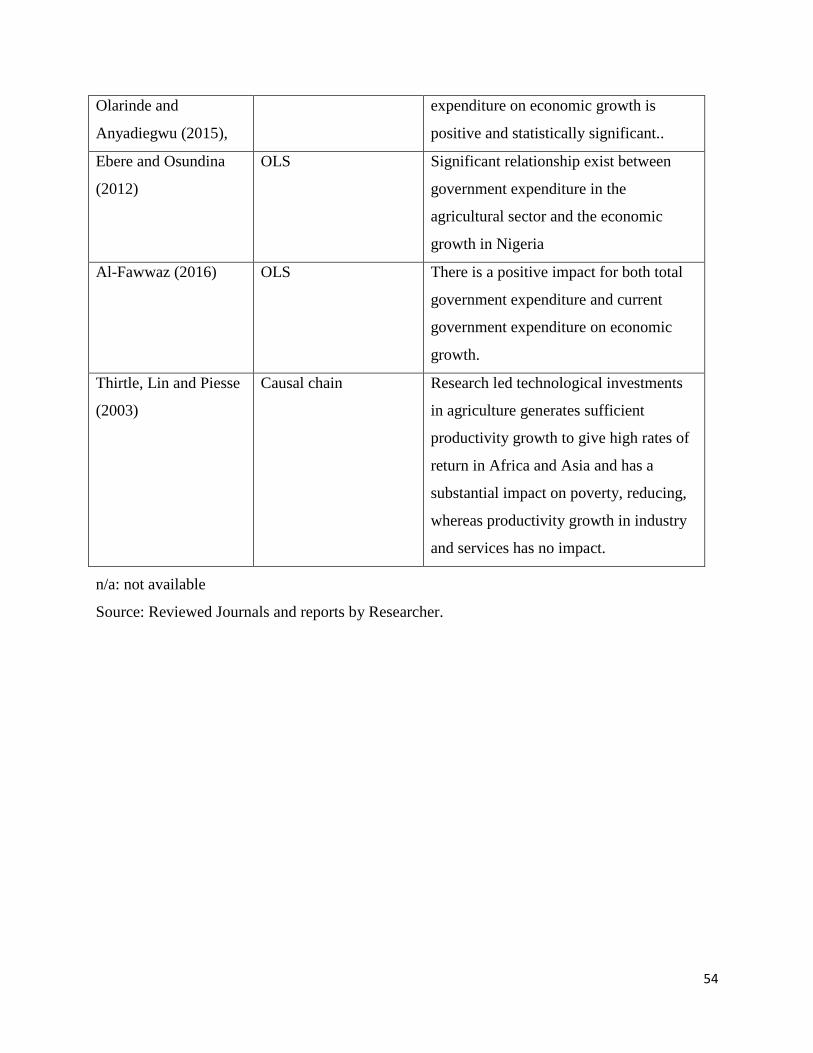
54

Olarinde and

Anyadiegwu (2015),

expenditure on economic growth is

positive and statistically significant..

Ebere and Osundina

(2012)

OLS Significant relationship exist between

government expenditure in the

agricultural sector and the economic

growth in Nigeria

Al-Fawwaz (2016) OLS There is a positive impact for both total

government expenditure and current

government expenditure on economic

growth.

Thirtle, Lin and Piesse

(2003)

Causal chain

Research led technological investments

in agriculture generates sufficient

productivity growth to give high rates of

return in Africa and Asia and has a

substantial impact on poverty, reducing,

whereas productivity growth in industry

and services has no impact.

n/a: not available

Source: Reviewed Journals and reports by Researcher.

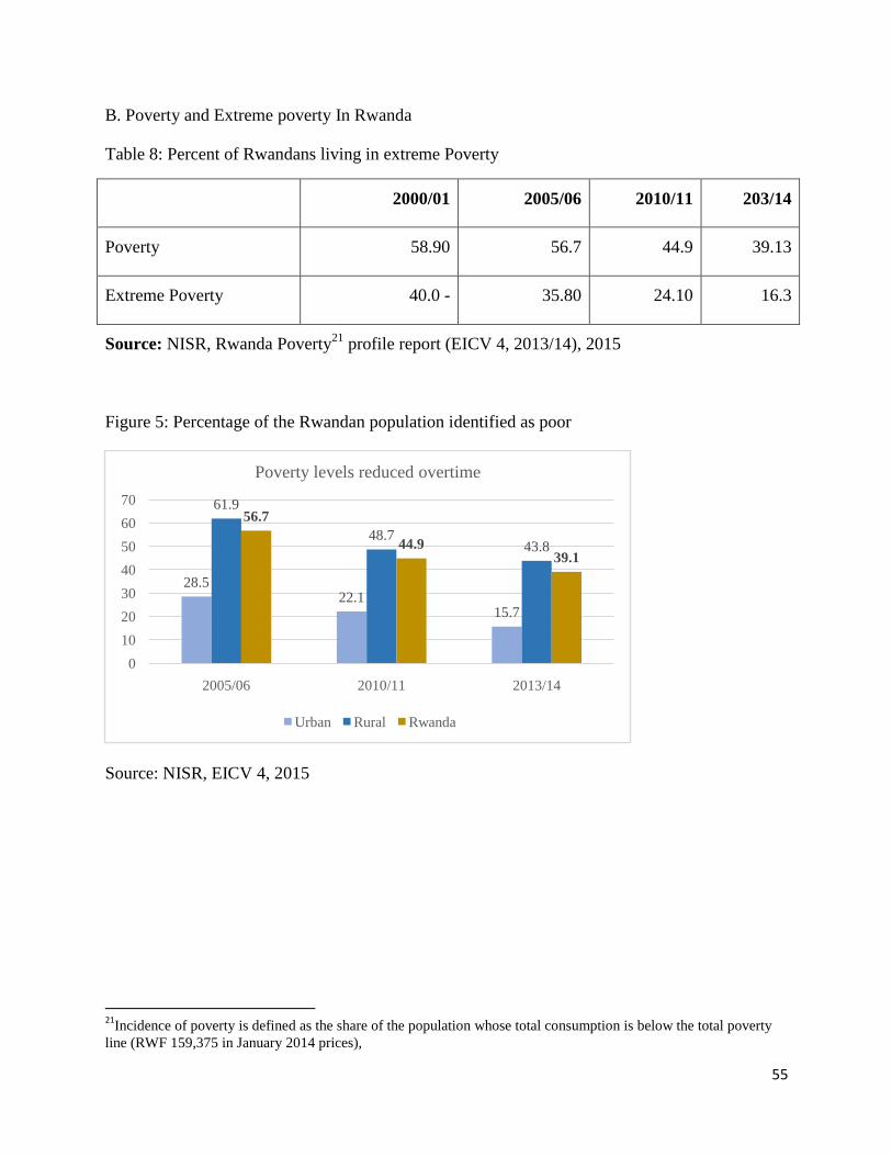
55

B. Poverty and Extreme poverty In Rwanda

Table 8: Percent of Rwandans living in extreme Poverty

2000/01 2005/06 2010/11 203/14

Poverty 58.90 56.7 44.9 39.13

Extreme Poverty 40.0 - 35.80 24.10 16.3

Source: NISR, Rwanda Poverty21

profile report (EICV 4, 2013/14), 2015

Figure 5: Percentage of the Rwandan population identified as poor

Source: NISR, EICV 4, 2015

21

Incidence of poverty is defined as the share of the population whose total consumption is below the total poverty

line (RWF 159,375 in January 2014 prices),

28.522.1

15.7

61.9

48.743.8

56.7

44.939.1

0

10

20

30

40

50

60

70

2005/06 2010/11 2013/14

Poverty levels reduced overtime

Urban Rural Rwanda

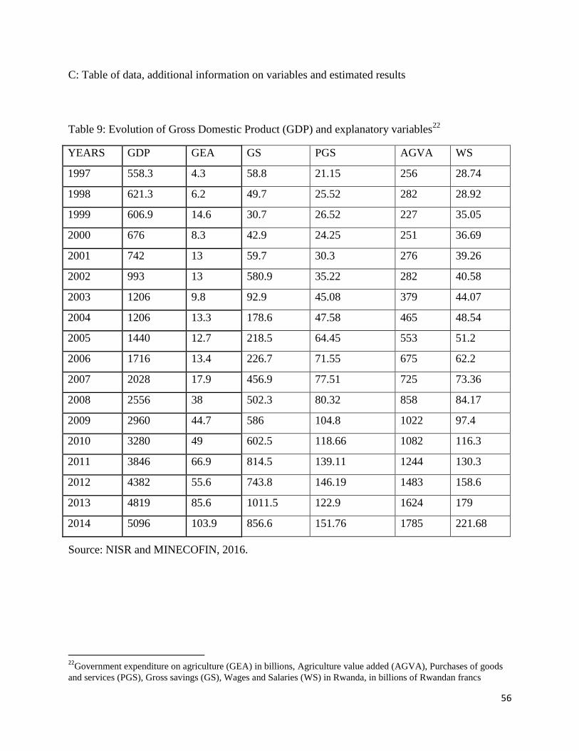
56

C: Table of data, additional information on variables and estimated results

Table 9: Evolution of Gross Domestic Product (GDP) and explanatory variables22

YEARS GDP GEA GS PGS AGVA WS

1997 558.3 4.3 58.8 21.15 256 28.74

1998 621.3 6.2 49.7 25.52 282 28.92

1999 606.9 14.6 30.7 26.52 227 35.05

2000 676 8.3 42.9 24.25 251 36.69

2001 742 13 59.7 30.3 276 39.26

2002 993 13 580.9 35.22 282 40.58

2003 1206 9.8 92.9 45.08 379 44.07

2004 1206 13.3 178.6 47.58 465 48.54

2005 1440 12.7 218.5 64.45 553 51.2

2006 1716 13.4 226.7 71.55 675 62.2

2007 2028 17.9 456.9 77.51 725 73.36

2008 2556 38 502.3 80.32 858 84.17

2009 2960 44.7 586 104.8 1022 97.4

2010 3280 49 602.5 118.66 1082 116.3

2011 3846 66.9 814.5 139.11 1244 130.3

2012 4382 55.6 743.8 146.19 1483 158.6

2013 4819 85.6 1011.5 122.9 1624 179

2014 5096 103.9 856.6 151.76 1785 221.68

Source: NISR and MINECOFIN, 2016.

22

Government expenditure on agriculture (GEA) in billions, Agriculture value added (AGVA), Purchases of goods

and services (PGS), Gross savings (GS), Wages and Salaries (WS) in Rwanda, in billions of Rwandan francs

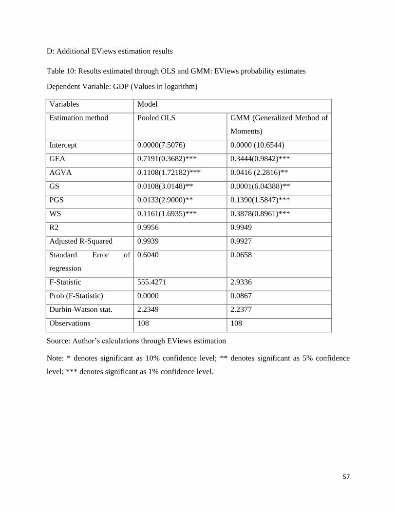
57

D: Additional EViews estimation results

Table 10: Results estimated through OLS and GMM: EViews probability estimates

Dependent Variable: GDP (Values in logarithm)

Variables Model

Estimation method Pooled OLS GMM (Generalized Method of

Moments)

Intercept 0.0000(7.5076) 0.0000 (10.6544)

GEA 0.7191(0.3682)*** 0.3444(0.9842)***

AGVA 0.1108(1.72182)*** 0.0416 (2.2816)**

GS 0.0108(3.0148)** 0.0001(6.04388)**

PGS 0.0133(2.9000)** 0.1390(1.5847)***

WS 0.1161(1.6935)*** 0.3878(0.8961)***

R2 0.9956 0.9949

Adjusted R-Squared 0.9939 0.9927

Standard Error of

regression

0.6040 0.0658

F-Statistic 555.4271 2.9336

Prob (F-Statistic) 0.0000 0.0867

Durbin-Watson stat. 2.2349 2.2377

Observations 108 108

Source: Author’s calculations through EViews estimation

Note: * denotes significant as 10% confidence level; ** denotes significant as 5% confidence

level; *** denotes significant as 1% confidence level.

Documents

Analysis of Government Spending on Agriculture Sector and