Analysis of Mesocyclone Detection Algorithm Attributes to Increase Tornado Detection

Christina M. Nestlerode1,2,3

and

Michael B. Richman4

Research Experience for Undergraduates Final Project

Last Revised: July 31, 2003

1OWC REU Program Norman, Oklahoma

2OU School of Meteorology

Norman, Oklahoma

3Lycoming College Department of Physics and Astronomy

700 College Place Box #1014

Williamsport, PA 17701 neschri@lycoming.edu

4The University of Oklahoma School of Meteorology 100 East Boyd Street Norman, OK 73019 mrichman@ou.edu

Abstract

The Mesocyclone Detection Algorithm (MDA) is used in the Weather Surveillance Radar

–1988 Doppler (WSR-88D) to detect rotation associated with tornadoes and other severe

weather. The MDA analyzes Doppler radar radial velocity volume scans to compose a number of

attributes thought to be related to mesocyclone formation. The 23 attributes of the MDA are

compared to truthed tornado data in exploratory and diagnostic analyses to examine the

underlying structure of the MDA.

Results of these analyses indicate that the MDA is a highly correlated system with a wide

variety of complexity in those correlations. This multicollinearity can hinder statistical

prediction. Measured associations between the attributes vary from near zero correlation to

complex correlations with values greater than 0.8, binding up to nine MDA attributes. In

diagnostic analyses, linear and logistic regressions are performed on various sets of MDA

attributes in an attempt to distinguish tornado events from non-tornado events. Logistic

regression is found to be the most successful model due to its parsimony and ability to classify

correctly tornado versus non-tornado cases.

This research has shown that the number of attributes in the MDA can be decreased by

projecting the 23 correlated attributes on a number of uncorrelated dimensions. Using principal

component analysis (PCA), multivariate exploration of the data determines that 9 dimensions are

needed to describe 85% of the variability of the MDA attributes. While the MDA is currently an

improvement over older algorithms, this research shows that it is advantageous to reduce the

redundancy of the MDA to make it a more useful tool.

1. Introduction

2

With the advent of a national network of Doppler radar capable of sensing small

circulation scales undiscovered until the last decade, the detection of mesocyclones has received

considerable attention in recent years. A mesocyclone can take on various definitions, one of

which is a storm-scale region of rotation, typically around 2-6 miles in diameter and often found

in the right rear flank of a supercell (Branick 2003). Alternatively, the term mesocyclone, as used

in Doppler radar studies, is defined as a rotation signature with measurable magnitude, vertical

depth, and duration (Branick 2003). Mesocyclones are of particular interest since tornadoes,

large hail, and damaging winds are collocated with the rotation area. These hazards lead to

unnecessary loss of life and destruction of property if people are not adequately warned of the

threat. Therefore, a significant proportion of mesocyclone studies (e.g. Desrochers and

Donaldson 1992, Lee and White 1998, Tipton et al. 1998, and Jones 2002) have addressed the

development of radar algorithms that can assist forecasters in predicting tornadoes and warning

people of imminent danger. Improvements in radar and algorithm technology have increased

lead time (time between the forecast of a tornado and its appearance) from a few minutes a

decade ago to eleven minutes in the past few years (Trafalis et al. 2003). Despite this, tornados

still kill and injure people due to insufficient warning time, misdetection, and complacency of

the public ignoring repeated false alarms (the number of tornadoes that an algorithm predicts that

fail to materialize). Additional lives will be saved if computer algorithms that identify

mesocyclones are improved; the goal of our project is to investigate the efficiency of the current

radar Mesocyclone Detection Algorithm. If the algorithm can be improved or simplified, that

should result in increased lead times and lower false alarm rates.

Detection algorithms exist within the Weather Surveillance Radar-1988 Doppler (WSR-

88D) system to find areas of rotation in severe thunderstorms. One of the algorithms, the

3

Mesocyclone Detection Algorithm (MDA), described by Stumpf et al. (1998), is in use to

replace the WSR-88D Build 9.0 Mesocyclone Algorithm (Zrnić et al. 1985). The older

algorithm, WSR-88D Build 9.0 Mesocyclone Algorithm (WSR-88D B9MA), has been found to

be incapable of detecting a number of mesocyclones because they are weaker than the threshold

strength of the algorithm, even though such rotations can produce tornadoes. Also, the WSR-

88D B9MA misclassifies many strong non-tornadic rotations by deducing tornado existence

within the rotation and hence, producing high false alarm rates in the range of 73.9 to 96.6

percent (Stumpf et al. 1998). The older algorithm looks for specific rotations as potentially

tornadic, whereas the MDA offers a new approach.

Stumpf et al. (1998) recognized that a new algorithm should detect storm rotations from

1-10 km in diameter to catch even seemingly insignificant rotation. Moreover, instead of instant

analysis of rotation, the MDA output scrutinizes each case for tornado development potential.

Other enhancements include new threshold definitions, improved vertical association, and the

introduction of association to features detected on radar volume scans.

Despite numerous improvements to the old algorithm, the MDA is not perfect. Trafalis et

al. (2003) state that the MDA has problems with the underdetection of tornadoes as well as the

high false alarm rate. Stumpf et al. (1998) calculate a false alarm rate for the MDA ranging from

67.7 to 75.7 percent. Furthermore, the MDA attributes have an unknown degree of redundancy,

since there are a large number of variables that comprise the MDA and many of them are

connected through Doppler velocity. It may be possible to reduce the number of attributes while

maintaining the accuracy of the MDA. By accomplishing such a goal, it will be easier for a

forecaster, who is under critical time constraint, to use the MDA more effectively in predicting

tornado formation.

4

Section 2 of this paper describes the data sets used. Section 3 discusses the variety of

methodologies that were applied in the research, Section 4 illustrates the results of the research,

and Section 5 presents the discussion of the results. The paper ends with Section 6, which is

conclusions from the research and suggestions for future lines of investigation.

2. Data

Two primary data sets are used in this research. The first is truthed tornado data collected

and verified by the National Severe Storms Laboratory (NSSL) through ground damage reports

(Stumpf et al. 1998). Twenty-three out of 24 MDA attributes measured for 2259 truthed tornado

cases are selected for the study. A second data set contains non-tornado data of the same 23

MDA attributes for 63,116 cases. The MDA attributes, defined by Stumpf et al. (1998), are

derived from Doppler radar radial velocity volume scans. Before the data are processed, artifacts

such as noise or incorrectly dealiased velocities in the volume scans are removed. All velocities

with reflectivity values below 20 dBZ are deleted and then an existing scheme within the WSR-

88D removes improperly dealiased velocities according to the threshold of the program (Eilts

and Smith 1990). The first step of the MDA creates shear segments by looking at cyclonic shear

patterns in the Doppler volume scans. Then, velocity difference and maximum gate-to-gate

velocity difference are calculated from the shear segments. The next step moves into 2-

dimensional (2D) analyses, and feature core extraction (Stumpf et al. 1998) is used to define

shear features horizontally. From these data, the rotational velocity of the detected vorticity

(rotation about a vertical axis) is computed. Then, a new vertical association technique is applied

to the 2D features to view the vortex in a 3-dimensional (3D) form. In the last step, a time

dimension is added to the 3D components if a feature appears on more than one consecutive

5

volume scan. From the MDA analyses, data used in this study contain 23 attributes, listed in

Table 1 (adapted from Trafalis et al. 2003) and described in Appendix A.

3. Methodology

The primary goals of the project are exploratory data analysis of the MDA as well as

diagnosis of tornado versus non-tornado events. Accordingly, it is important to compare directly

tornado cases and non-tornado cases. From the non-tornado data, 2259 cases are randomly

selected to have the same number of observations as the tornado data set. By creating a data set

with as many tornadoes as non-tornadoes, the techniques applied to these data have the

opportunity to be unbiased.

Exploratory data analysis is carried out at the univariate, bivariate, and multivariate

levels. All analyses are performed using S-Plus 2000. For univariate analyses, histograms of the

tornado and non-tornado cases are created. For comparison purposes, each attribute is plotted on

the same scale for both data sets, making it possible to overlay and compare the histograms for

tornado and non-tornado cases. Bivariate data analysis of the MDA attributes is carried out by

visual inspection of scatterplots and through calculation of Pearson correlations. Multivariate

analysis makes use of principal components (PC) to discover the underlying number of

dimensions of the MDA and the correlation structure of these dimensions. The fundamental

equation of principal component analysis (PCA) is Z = FAT where Z is a matrix of the

standardized MDA data of order n x m where n is the number of cases and m is the number of

attributes, F is the matrix of the PC score time series of order n x p where p is the number of PCs

retained, and A is the matrix of the PC loadings that portray which attributes cluster together on

each dimension. The matrix A is of order m x p (Richman 1986). PCA is performed in multiple

steps. The first step involves relating the data. Since the MDA data are measured on different

6

metrics, they are standardized implicitly by forming a 23 x 23 correlation matrix, R. The

correlation matrix is decomposed into eigenvectors, V, and eigenvalues, D, according to the

following equation R = AAT where A = VD½. Since the goal is the compact description of the

MDA’s correlation structure, a Varimax orthogonal rotation is applied to determine which

attributes cluster on specific dimensions. The second step involves determining the optimal

number of PC dimensions (p) to rotate based on minimizing the number of misclassifications of

the clustering of attributes as depicted in R. A plausible range of solutions is identified for

p = 4,5,…,10 and each solution is tested for the number of misclassified attributes. The

classification process is defined by binarizing the rotated PC loadings where a loading with an

absolute value ≥0.5 is considered “in the cluster” and coded as 1. Those loadings with an

absolute value < 0.5 are considered “out of the cluster” and coded as 0. The philosophy behind

this approach is given in Richman and Gong (1999). Similarly, those values in R with an

absolute value 0.5 are considered in the cluster and those correlations with an absolute value <

0.5 are considered out of the cluster and coded as 1 and 0, respectively. In cases where a 0 in the

loadings are matched to a 1 in the correlations or vice versa, these are coded as

misclassifications. The dimension number associated with the lowest number of

misclassifications is selected as the optimal p.

≥

Another way of assessing misclassification is through the use of regression. Linear and

logistic regressions are applied to the 23 MDA attributes. Linear regression is used as a baseline

to determine the amount of linear relation between the attributes in discriminating tornadoes

from non-tornadoes, whereas, logistic regression is a non-linear type of regression where the

dependant variable is a dummy variable labeled 0 or 1. If the event occurs, the variable is one

number, if it does not, the variable is the other number. In this way, data with only two outcomes

7

can be analyzed easily (Wilks 1995). A stepwise process is used to preprocess the linear

regression by eliminating those attributes that do not provide significant residual sum of squares

(RSS) to the variance explained. Those attributes with significant RSS, as tested by an t-statistic,

are retained and inserted into the linear regression model. A similar process is used to reduce the

number of MDA attributes in the logistic regression based on the amount of deviance explained.

Those attributes with significant deviance are retained and inserted into the logistic regression

model that is analyzed physically. Another measure of regression model performance is R2

(Wilks 1995). The counterpart to R2 for logistic regression is called the pseudo R2, defined as

1-(Residual Deviance/Null Deviance). A standardization preprocessing is performed on the data

before the logistic regression. The data are scaled by shifting each attributes mean to zero, the

variance to be one, and the skew to be close to zero. After the standardization procedure, Box-

Cox transformations are performed on the data to remove skewness and help meet the

distributional assumptions of the regression. For testing purposes, the tornado data was split into

two parts. The first half is used as training data to select a model to predict the second half using

both linear and logistic regressions. Likewise, the second half is used as training data to predict

the first half. By doing so, the stability of the model coefficients can be examined.

Misclassification analysis is applied to the regressions in the following process. The

predictions of the regressions are binarized (1,0) where a 1 represents a tornado prediction and a

0 represents a non-tornado prediction. These are compared directly to the truthed data and

tallied.

8

4. Results

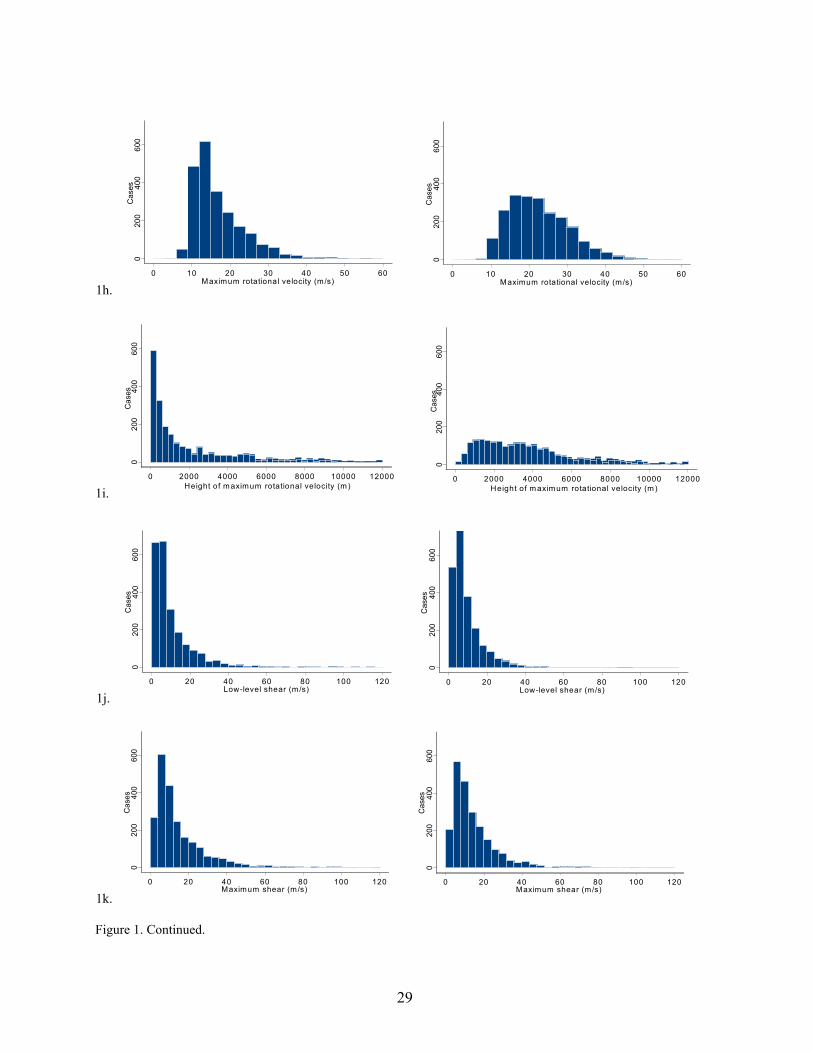
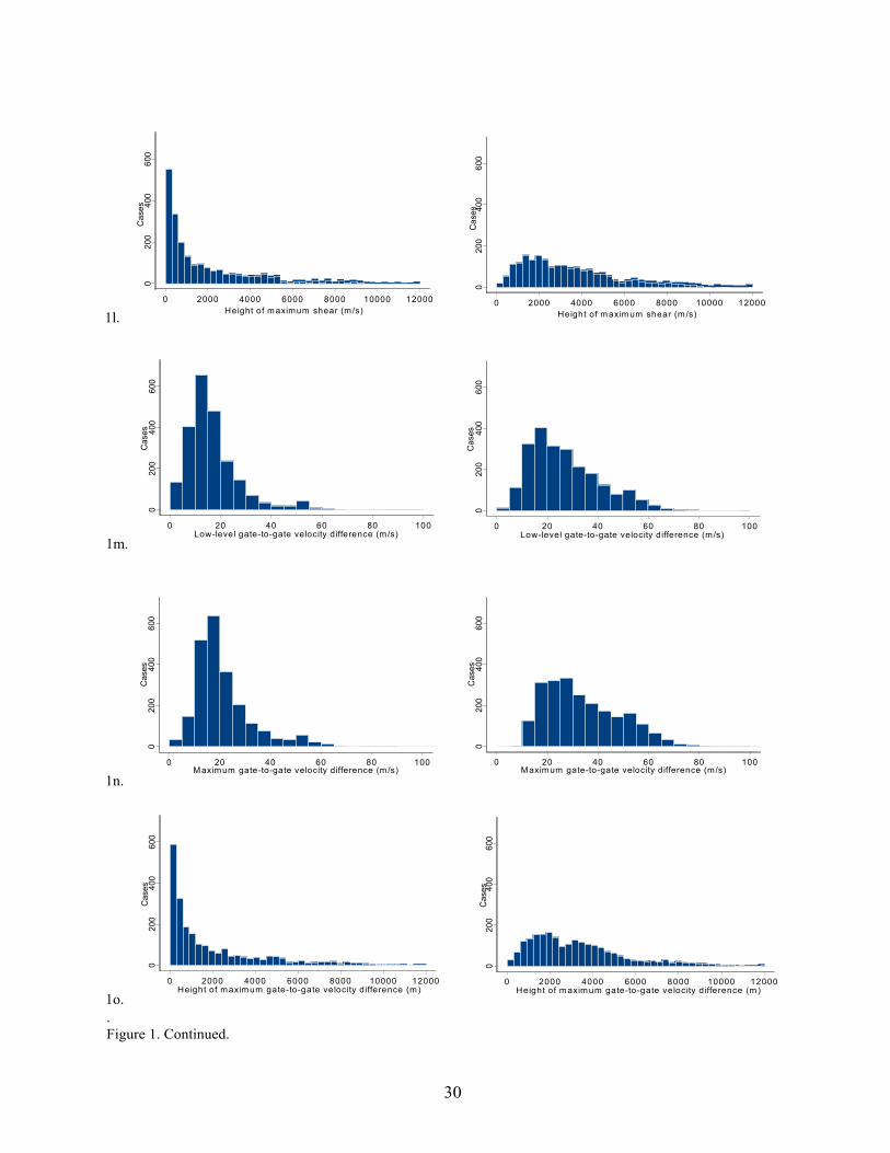
Histograms provide basic information on the shape of the distributions for the tornado

and non-tornado data sets (Figure 1). When visually assessing histograms showing the radar

detected mesocyclone base, there is a striking difference between the two data sets (Figure 1a).

The non-tornado cases (left column) are dominated by bases at 400 m or less whereas tornado

cases have a more even distribution of base heights, with a maximum around 1000 m. There is a

considerable amount of overlap between the distributions for the two sets. Comparison of the

depth (Figure 1b) show most of the non-tornado cases at depths less than 2000 m, as opposed to

the tornado cases that exist in the range of approximately 2000 to 12000 m. When looking at

strength rank (Figure 1c), there is considerable overlap between the two sets from ranks 1 to 6.

The zero rank is mainly comprised of non-tornadoes while ranks above 5 are generally tornado

cases. In low-level diameter (Figure 1d), there is a large amount of overlap between the two sets.

There is a greater number of non-tornadoes at small low-level diameters than tornadoes. At least

half of the distribution overlaps in maximum diameter (Figure 1e). Despite the overlap in the

right tails of the two sets, many of the non-tornado cases heights of maximum diameter (Figure

1f) occur at below 2000 m. There is less low-level rotational velocity in the non-tornado cases,

but there is a large overlap between the distributions of the two sets (Figure 1g). Similar results

can be seen for maximum rotational velocity (Figure 1h). Histograms of the height of maximum

rotational velocity (Figure 1i), show a broad maximum in the tornado cases between 1000 and

4000 m. In low-level shear and maximum shear, the two distributions are almost identical

(Figures 1j and 1k). Similar to Figure 1i, height of maximum shear (Figure 1l) shows a spike in

the non-tornado cases at values lower than 2000 m, and a broad maximum for tornado cases

from 500 to 4000 m. Low-level gate-to-gate velocity difference (Figure 1m) indicates less

9

overlap than shear, and the non-tornado cases seem to decrease after 30 ms-1, while the tornado

cases are evident until 55 ms-1. Maximum gate-to-gate velocity difference (Figure 1n) shows that

the two distributions are offset more than in the low-level gate-to-gate velocity difference

distributions. Non-tornado cases are scarce after 40 ms-1 whereas tornado cases appear until 65

ms-1. Height of maximum gate-to-gate velocity difference (Figure 1o) shows a peak in non-

tornado cases below 2000 m. Core base histograms (Figure 1p) illustrate similarities to previous

height parameters, but there are fewer non-tornado cases in the mid levels. Core depth (Figure

1q) is striking as no tornado cases occur below 3000 m, while a majority of the non-tornado

cases are at less than 2000 m. The shape of the distribution of tornado cases and non-tornado

cases is similar when looking at age (Figure 1r), but non-tornadoes decrease rapidly in number

after 30 min while some tornado cases exist up to 100 min. Strength index is an attribute that

shows overlap between the two data sets with some separation below 2000 m and above 4000 m

(Figure 1s). Strength index “rank” has considerable overlap in ranks from 0 to 3, however, there

are many more tornado cases with ranks greater than 4 (Figure 1t). Figure 1u depicts that tornado

cases have significant relative depth when compared with non-tornado cases. There is some

overlap in the middle of the distributions, but the left part of the distribution illustrates a striking

peak in non-tornado cases. Low-level and mid-level convergence are unique attributes because

they are both bimodal. However, low-level convergence (Figure 1v) shows a peak in non-

tornadoes at lower values if the zeros are ignored, whereas mid-level convergence shows an

overlap between the two sets (Figure 1w).

Bivariate analysis though scatterplots indicated a large range of associations between the

pairs of MDA variables (not shown). Many of the 23 MDA attributes are highly correlated

within the tornado and non-tornado data sets. In the tornado data set (Table 2), Pearson

10

correlation calculations establish strong relationships (defined as absolute correlations exceeding

0.75), especially between the three strength parameters (attributes 3, 19, 20), rotational velocities

(attributes 7 and 8), and gate-to-gate velocity differences (attributes 13 and 14). In the non-

tornado cases (Table 3), a greater number of high correlations occur with emphasis on height

parameters (attributes 6, 9, 12, 15, and 16). There are inherent differences in the correlation

structures of the tornado and non-tornado data. For example, the tornado data shows correlations

between base, core base, and a negative relationship with low-level convergence, while in the

non-tornado cases, base is related to depth, strength rank, height of maximum diameter, height of

maximum rotational velocity, height of maximum shear, height of maximum gate-to-gate

velocity difference, core depth, relative depth and low-level divergence.

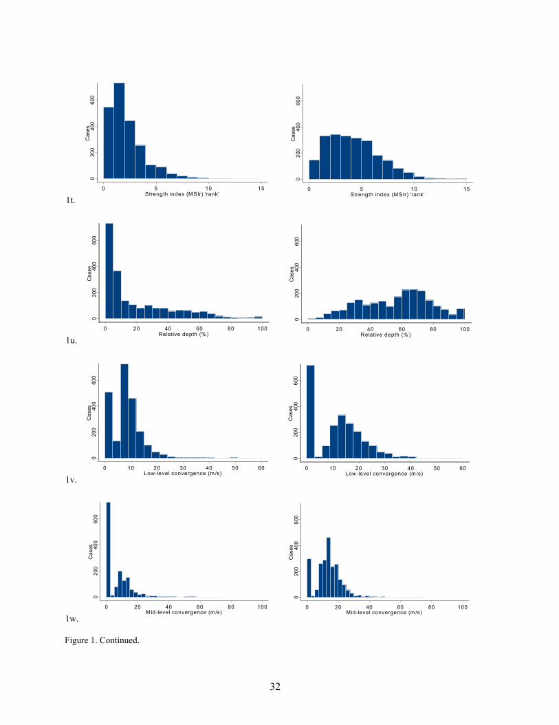
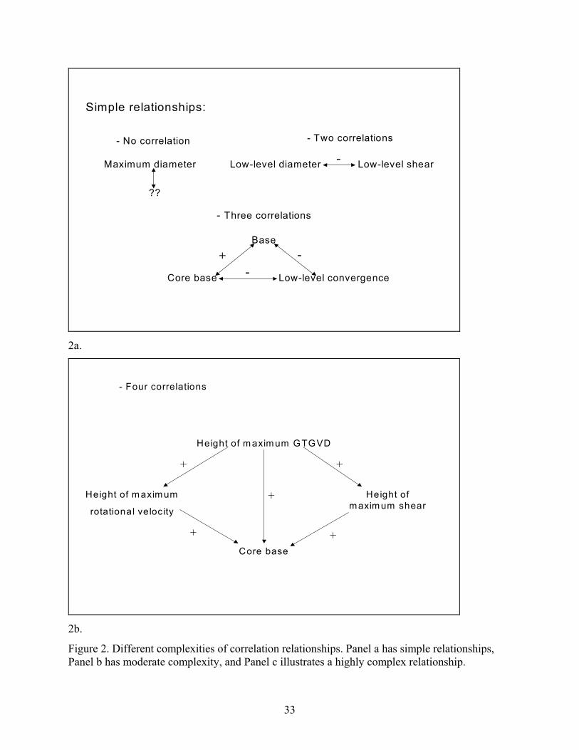
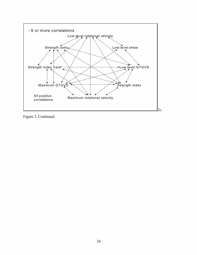
There is a range in complexity of the underlying correlation structure of the data. As seen

in Figure 2a, some attributes are not correlated with any others. The complexity then increases,

as some attributes are correlated with one other, some are associated with two others, and some

are related to four other attributes (Figure 2b). The most complex case involves more than eight

variables where most are associated with all other attributes (Figure 2c).

Multivariate analysis using PCA determines how many underlying attributes are needed

to account for a substantial proportion of the variability of the MDA attributes and to summarize

the correlation structure of the attributes. For the tornado cases, the optimal p is found to be 9

with one misclassification (Table 4). With 9 dimensions, 85 percent of the total MDA variance is

represented using only 39 percent of the data. The variables that cluster together for PC 1

through 9 are shown (Table 6). On the first PC are strength rank, low-level rotational velocity,

maximum rotational velocity, low-level shear, maximum shear, low-level gate-to-gate velocity

difference, maximum gate-to-gate velocity difference, strength index and strength index “rank”.

11

Since some of the velocity parameters are used to define the strength indices and ranks (see

Appendix A), this PC is loading the attributes related to “circulation strength”. The second PC

accounts for “circulation base characteristics” as it contains base, core base, and negative low-

level convergence. The third PC is depth, height of maximum diameter, and relative depth, so it

is a measure of “circulation volume”. Low-level shear and negative low-level diameter comprise

the fourth PC and represent the “low-level circulation” characteristics of the storm. The fifth PC

is a “circulation height” measure as it contains height of maximum rotational velocity, height of

maximum shear, height of maximum gate-to-gate velocity difference, and core base. PCs 6

through 9 are associated with single attributes and can be named accordingly. The sixth PC

loads only age. Core depth comprises the seventh PC, mid-level convergence is on the eighth

PC, and maximum diameter loads on the ninth PC. Each of the nine PCs have an associated PC

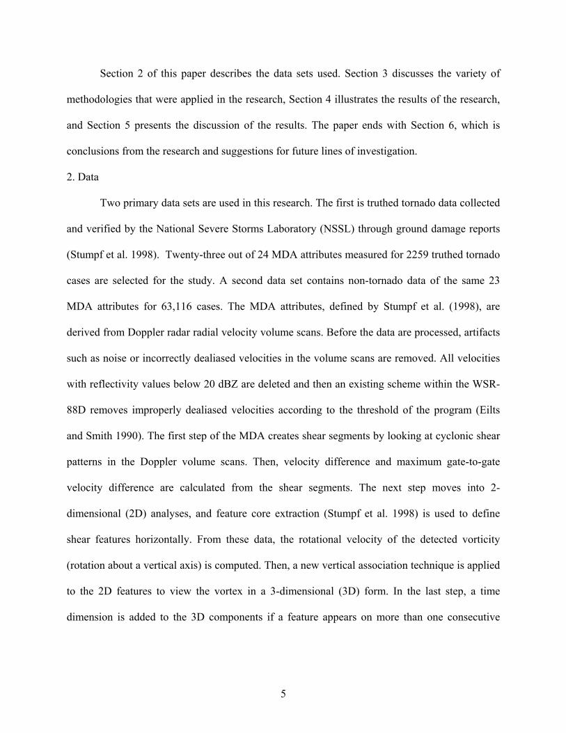
score that described the time behavior of each cluster of attributes (PCs 1 – 5) or single attributes

(PCs 6 -9). Any individual tornado can therefore be profiled by examining the PC scores for that

case. By doing so, it is possible to distinguish tornadoes with greater than average low level

circulation from those with large circulation volume (Figure 3).

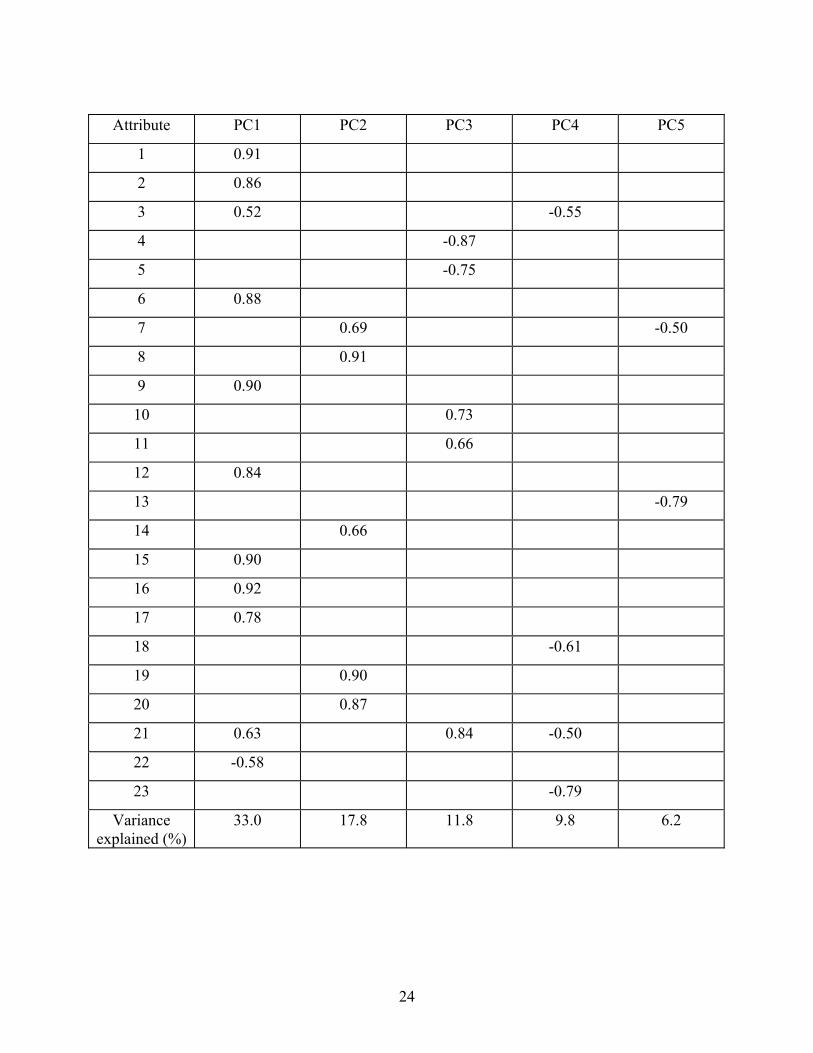
The optimal p for the non-tornado cases is 5 and that is associated with 6

misclassifications. Five dimensions account for 78.5 percent of the variance of the MDA

attributes and only 21.7 percent of the data. Other dimensions are analyzed, but they have more

misclassification as seen in Table 5. The first PC is a representation of “depth and height” of the

non-tornado cases since it contains base, depth, strength rank, height of maximum diameter,

height of maximum rotational velocity, height of maximum shear, height of maximum gate-to-

gate velocity difference, core base, core depth, relative depth, and low-level convergence (Table

7). The second PC is composed of low-level rotational velocity, maximum rotational velocity,

12

maximum gate-to-gate velocity difference, strength index, and strength index “rank”, so it

represents strength. Negative low-level diameter and maximum diameter load with low-level

shear and maximum shear on the third PC, making it a glimpse of low-level characteristics of the

storm. The fourth PC has strength rank, age, relative depth, and mid-level convergence, so it

shows the weakness of the mesocyclone. The fifth PC is a velocity parameter, since it loads low-

level rotational velocity and low-level gate-to-gate velocity difference.

The regression analyses combine the tornado and non-tornado data to diagnose which

attributes (known as predictors) are best suited to distinguishing between the two. Twelve

significant linear regression attributes are determined using the t-test (Table 8). The most

significant attribute according the t-statistic is strength rank. Age, core depth, and relative depth

also predict the variance well, with high t-values. In linear regression, the R2 of the first half of

the data predicting the second half is 0.5666. Using the second half to predict the first half, the

R2 value is 0.5456. In logistic regression, the nine most important attributes are determined

through explained deviance. Table 9 shows that the most significant attributes are strength rank,

age and base, all with t-values above 5 (highly significant). The pseudo R2 for the first half of the

data predicting the second half is 0.5306 and 0.5105 for the second half of the data predicting

the first. All of the attributes in logistic regression also appear in linear regression, but linear

includes maximum rotational velocity, height of maximum rotational velocity, and height of

maximum gate-to-gate velocity difference. In the ability to distinguish correctly tornadoes from

non-tornadoes, logistic regression has better results than linear regression by .6 percent (Table

10). Logistic regression is considered the superior technique because it is a more accurate

classifier and uses fewer predictors to achieve that level of classification.

13

5. Discussion

The histogram results show a number of important features of the MDA, especially

concerning attributes whose distributions between tornado and non-tornado cases do not separate

well. Low-level diameter is not a good discriminator because there is a extensive overlap

between the two data sets. Similarly, low-level rotational velocity, maximum rotational velocity,

low-level shear, maximum shear, low-level gate-to-gate velocity difference, maximum gate-to-

gate velocity difference, and strength index have significant overlap in the distributions of the

two cases. Interestingly, low-level shear and maximum shear histograms are almost identical,

meaning that there is no need for two separate discriminators of shear. Another intriguing feature

of the MDA attributes are the height parameters. There are prominent peaks in the non-tornado

cases of base, height of maximum diameter, height of maximum rotational velocity, height of

maximum shear, height of maximum gate-to-gate velocity difference, core base, and relative

depth. Tornadoes tend to occur with higher bases, maximum diameters, and core bases; they also

tend to have velocity components higher in the storm. There is also a broader range of heights in

tornado cases. Another promising discriminator is core depth because there is a striking lack of

overlap in the histograms of the two data sets. In tornado cases, core depth is almost always

above 3000 m while non-tornado storms have core depths below 2000 m. Age has almost a

complete overlap between the two sets, but tornado cases to tend to last longer because they may

survive for up to 100 minutes while non-tornado features last no longer than 30 minutes.

Strength rank and strength index “rank” histograms are similar because tornadoes have strengths

much higher than non-tornadoes do.

The PCA results are consistent with the correlation matrix since the same variables are

correlated as those that are grouped on a PC. For example, the correlation matrix shows that

14

height of maximum rotational velocity, height of maximum shear, height of maximum GTGVD,

and core base are all highly positively associated and the same group of attributes represents the

second PC. Also, the regression results pull out the same significant variables as the correlation

matrix and the PCA. The two sets of regression results are stable; therefore, this leads credence

to the models being stable.

6. Conclusions

The correlation results suggest that the MDA is overdetermined and complex in that most

of the attributes are associated strongly with each other. The PCA has the ability to draw the

meaningful structures out of the complicated correlation matrix. Twenty three attributes are

replaced by 9 orthogonal dimensions resulting in a more compact conceptual model of the MDA.

Interestingly, the number of dimensions given by the PCA is same as the number of predictors

given by the logistic regression. Each rotated PC is interpreted as a physically meaningful

structure that relates well to the clusters of variables in the parent correlation matrix. These, in

turn, relate to rotation of the atmosphere. Furthermore, the PC model provides a time series of

each of these new dimensions. Individual tornado profiles are a unique classification tool,

showing the tornado’s strengths and weaknesses in the range of each PC. The combination of PC

loadings, identifying clusters of highly correlated MDA attributes for physical interpretation and

PC scores that express the time behavior of the new uncorrelated variables, offers an exciting

line of investigation in profiling tornadic events based on which types of atmospheric behavior

are associated with different types of storms. Based on the consistency among several types of

statistical investigations, the results suggest that the MDA can be simplified without loss of

accuracy.

15

Acknowledgements: This work was funded by National Science Foundation grant NSF 0097651.

A portion of Dr. Richman’s time was supported by NSF Grant EIA-0205628. The lead author

would like to thank Daphne Zaras and the REU selection committee, Greg Stumpf at NSSL for

his support and patience, Philip Bothwell and Kim Elmore for help with S-Plus, Becca Mazur for

her support with Quality Control, Mark Laufersweiler for help and advice, and all of the

REU/ORISE/SCEP students who made the summer as extreme as possible.

Appendix A

The 23 MDA attributes are measurements gleaned from Doppler radial velocity data.

Base is the height above radar level (ARL) of the lowest 2D elevation scan. By adding half-

power beamwitdth to the top and bottom of the final 3D feature, depth is calculated. Strength

rank is a dimensionless number ranging from 1 to 25 that is first applied to the 1D shear

segments, and later adjusted after the 2D elevation scans are analyzed. The strength of the

vortex is determined by preset thresholds in velocity difference and shear, or gate-to-gate

velocity difference based on Philips Laboratory and early MDA criteria. Low-level diameter (D)

is the distance between the maximum outbound velocity (Vmax) and maximum inbound velocity

(Vmin) at the lowest 2D elevation scan. Maximum diameter is the distance between Vmax and

Vmin at the greatest diameter from all features below 12 km. Height of maximum diameter is the

altitude at which the maximum diameter is measured. Low-level rotational velocity (Vr) is (Vmax-

Vmin)/2 at the lowest altitude 2D elevation scan. Maximum rotational velocity is the highest

value of (Vmax- Vmin)/2 through all volume scans. Height of maximum rotational velocity is the

altitude at which the maximum rotational is found. Low-level shear is Vr /D at the lowest 2D

feature. Maximum shear is the highest value of Vr /D. Height of maximum shear is the altitude at

which maximum shear is measured. Low-level gate-to-gate velocity difference (GTGVD) is the

16

lowest elevation scan measure of greatest velocity difference between adjacent velocity values in

the original shear segment. The greatest GTGVD in the whole storm is the maximum GTGVD.

Where maximum GTGVD is measured is the height of maximum GTGVD. Core base and core

depth are the measures of the lowest elevation scan ARL and the depth at the determined vertical

core, which is defined by its strength rank. Age is the fourth dimension of the MDA output; it is

a measure of the amount of time that the rotation exists. Mesocyclone Strength Index (MSI) is a

strength index that is measured by integrating the previously determined strength ranks and

multiplying by 1000. Each strength rank is weighted based on air density so that more emphasis

is given to 2D features at lower heights. The MSI is normalized by dividing it by the total depth

of the 3D feature. Strength index (MSIr) “rank” is a non-dimensional number ranging from 1 to

25 to correct to the strength index for range sampling limitations. Relative depth is an attribute

taken from the NSSL SCIT algorithm (Johnson et al. 1998) or sounding data and it is the

percentage of the depth of the storm cell. Low-level and mid-level convergence are measured

from the average of the radial convergence shear segment velocity differences in the 2D features

(adapted from Stumpf et al. 1998).

17

References

Branick, M., cited 2003: A Comprehensive Glossary of Weather Terms for Storm Spotters. [Available online at http://www.srh.noaa.gov/oun/severewx/glossary.php.] Desrochers, P. R. and R. J. Donaldson, 1992: Automatic Tornado Prediction with an Improved Mesocyclone-Detection Algorithm. Weather and Forecasting, 7, 373–388. Eilts, M. D., and S. D. Smith, 1990: Efficient Dealiasing of Doppler Velocities Using Local Environment Constraints. Journal of Atmospheric and Oceanic Technology, 7, 118-128. Johnson, J. T., P. L. MacKeen, A. Witt, E. D. Mitchell, G. J. Stumpf, M. D. Eilts, K. W. Thomas, 1998: The Storm Cell Identification and Tracking Algorithm: An Enhanced WSR-88D Algorithm. Weather and Forecasting, 13, 263–276. Jones, T. A., 2002: Verification of the NSSL Mesocyclone Detection Algorithm: A Climatological Perspective. Unpublished MS Thesis, University of Oklahoma, Norman, OK, 235pp. Lee, R. R., and A. White, 1998: Improvement of the WSR-88D Mesocyclone Algorithm. Weather and Forecasting, 2, 341–351. Richman, M. B., 1986: Rotation of Principal Components. Journal of Climatology, 6, 293-335. Richman, M.B, and X. Gong, 1999: Relationships between the Definition of the Hyperplane Width to the Fidelity of Principal Component Loading Patterns. Journal of Climate, 12, 1557-1576. Stumpf, G. J., A. Witt, E. D. Mitchell, P. L. Spencer, J. T. Johnson, M. D. Eilts, K. W. Thomas, and D. W. Burgess, 1998: The National Severe Storms Laboratory Mesocyclone Detection Algorithm for the WSR-88D. Weather and Forecasting, 13, 304-326. Tipton, G. A., E. D. Howieson, J. A. Margraf, and R. R. Lee, 1998: Optimizing the WSR-88D Mesocyclone/Tornadic Vortex Signature Algorithm using WATADS—A case study*. Weather and Forecasting, 3, 367–376. Trafalis, T.B., B. Santosa and M.B. Richman, 2003: Tornado detection with kernel-based methods. Intelligent Engineering Systems Through Artificial Neural Networks, ASME Press, 13, in press. Wilks, D. S., 1995: Statistical Methods in the Atmospheric Sciences. R. Dmowska and J. R. Holton, Academic Press, 160-181. Zrnić, D. S., D. W. Burgess, and L. D. Hennington, 1985: Automatic detection of mesocyclonic shear with Doppler radar. Journal of Atmospheric and Oceanic Technology, 2, 425-438. Table 1. List of 23 Mesocyclone Detection Algorithm attributes.

18

1. base (m) [0-12000] 13. low-level gate-to-gate velocity difference (m/s) [0-130]

2. depth (m) [0-13000] 14. maximum gate-to-gate velocity difference (m/s) [0-130]

3. strength rank [0-25] 15. height of maximum gate-to-gate velocity difference (m) [0-12000]

4. low-level diameter (m) [0-15000] 16. core base (m) [0-12000] 5. maximum diameter (m) [0-15000] 17. core depth (m) [0-9000] 6. height of maximum diameter (m) [0-12000] 18. age (min) [0-200] 7. low-level rotational velocity (m/s) [0-65] 19. strength index (MSI) weighted by average

density of integrated layer [0-13000] 8. maximum rotational velocity (m/s) [0-65] 20. strength index (MSIr) “rank” [0-25] 9. height of maximum rotational velocity (m) [0-12000]

21. relative depth (%) [0-100]

10. low-level shear (m/s/km) [0-175] 22. low-level convergence (m/s) [0-70] 11. maximum shear (m/s/km) [0-175] 23. mid-level convergence (m/s) [0-70] 12. height of maximum shear (m) [0-12000]

19

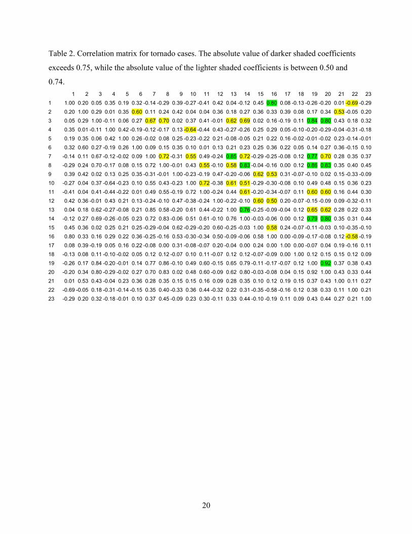
Table 2. Correlation matrix for tornado cases. The absolute value of darker shaded coefficients

exceeds 0.75, while the absolute value of the lighter shaded coefficients is between 0.50 and

0.74. 1 2 3 4 5 6 7 8 9 10 11 12 13 14 15 16 17 18 19 20 21 22 231 1.00 0.20 0.05 0.35 0.19 0.32 -0.14 -0.29 0.39 -0.27 -0.41 0.42 0.04 -0.12 0.45 0.80 0.08 -0.13 -0.26 -0.20 0.01 -0.69 -0.292 0.20 1.00 0.29 0.01 0.35 0.60 0.11 0.24 0.42 0.04 0.04 0.36 0.18 0.27 0.36 0.33 0.39 0.08 0.17 0.34 0.53 -0.05 0.203 0.05 0.29 1.00 -0.11 0.06 0.27 0.67 0.70 0.02 0.37 0.41 -0.01 0.62 0.69 0.02 0.16 -0.19 0.11 0.84 0.80 0.43 0.18 0.324 0.35 0.01 -0.11 1.00 0.42 -0.19 -0.12 -0.17 0.13 -0.64 -0.44 0.43 -0.27 -0.26 0.25 0.29 0.05 -0.10 -0.20 -0.29 -0.04 -0.31 -0.185 0.19 0.35 0.06 0.42 1.00 0.26 -0.02 0.08 0.25 -0.23 -0.22 0.21 -0.08 -0.05 0.21 0.22 0.16 -0.02 -0.01 -0.02 0.23 -0.14 -0.016 0.32 0.60 0.27 -0.19 0.26 1.00 0.09 0.15 0.35 0.10 0.01 0.13 0.21 0.23 0.25 0.36 0.22 0.05 0.14 0.27 0.36 -0.15 0.107 -0.14 0.11 0.67 -0.12 -0.02 0.09 1.00 0.72 -0.31 0.55 0.49 -0.24 0.85 0.72 -0.29 -0.25 -0.08 0.12 0.77 0.70 0.28 0.35 0.378 -0.29 0.24 0.70 -0.17 0.08 0.15 0.72 1.00 -0.01 0.43 0.55 -0.10 0.58 0.83 -0.04 -0.16 0.00 0.12 0.86 0.83 0.35 0.40 0.459 0.39 0.42 0.02 0.13 0.25 0.35 -0.31 -0.01 1.00 -0.23 -0.19 0.47 -0.20 -0.06 0.62 0.53 0.31 -0.07 -0.10 0.02 0.15 -0.33 -0.0910 -0.27 0.04 0.37 -0.64 -0.23 0.10 0.55 0.43 -0.23 1.00 0.72 -0.38 0.61 0.51 -0.29 -0.30 -0.08 0.10 0.49 0.48 0.15 0.36 0.2311 -0.41 0.04 0.41 -0.44 -0.22 0.01 0.49 0.55 -0.19 0.72 1.00 -0.24 0.44 0.61 -0.20 -0.34 -0.07 0.11 0.60 0.60 0.16 0.44 0.3012 0.42 0.36 -0.01 0.43 0.21 0.13 -0.24 -0.10 0.47 -0.38 -0.24 1.00 -0.22 -0.10 0.60 0.50 0.20 -0.07 -0.15 -0.09 0.09 -0.32 -0.1113 0.04 0.18 0.62 -0.27 -0.08 0.21 0.85 0.58 -0.20 0.61 0.44 -0.22 1.00 0.76 -0.25 -0.09 -0.04 0.12 0.65 0.62 0.28 0.22 0.3314 -0.12 0.27 0.69 -0.26 -0.05 0.23 0.72 0.83 -0.06 0.51 0.61 -0.10 0.76 1.00 -0.03 -0.06 0.00 0.12 0.79 0.80 0.35 0.31 0.4415 0.45 0.36 0.02 0.25 0.21 0.25 -0.29 -0.04 0.62 -0.29 -0.20 0.60 -0.25 -0.03 1.00 0.58 0.24 -0.07 -0.11 -0.03 0.10 -0.35 -0.1016 0.80 0.33 0.16 0.29 0.22 0.36 -0.25 -0.16 0.53 -0.30 -0.34 0.50 -0.09 -0.06 0.58 1.00 0.00 -0.09 -0.17 -0.08 0.12 -0.58 -0.1917 0.08 0.39 -0.19 0.05 0.16 0.22 -0.08 0.00 0.31 -0.08 -0.07 0.20 -0.04 0.00 0.24 0.00 1.00 0.00 -0.07 0.04 0.19 -0.16 0.1118 -0.13 0.08 0.11 -0.10 -0.02 0.05 0.12 0.12 -0.07 0.10 0.11 -0.07 0.12 0.12 -0.07 -0.09 0.00 1.00 0.12 0.15 0.15 0.12 0.0919 -0.26 0.17 0.84 -0.20 -0.01 0.14 0.77 0.86 -0.10 0.49 0.60 -0.15 0.65 0.79 -0.11 -0.17 -0.07 0.12 1.00 0.92 0.37 0.38 0.4320 -0.20 0.34 0.80 -0.29 -0.02 0.27 0.70 0.83 0.02 0.48 0.60 -0.09 0.62 0.80 -0.03 -0.08 0.04 0.15 0.92 1.00 0.43 0.33 0.4421 0.01 0.53 0.43 -0.04 0.23 0.36 0.28 0.35 0.15 0.15 0.16 0.09 0.28 0.35 0.10 0.12 0.19 0.15 0.37 0.43 1.00 0.11 0.2722 -0.69 -0.05 0.18 -0.31 -0.14 -0.15 0.35 0.40 -0.33 0.36 0.44 -0.32 0.22 0.31 -0.35 -0.58 -0.16 0.12 0.38 0.33 0.11 1.00 0.2123 -0.29 0.20 0.32 -0.18 -0.01 0.10 0.37 0.45 -0.09 0.23 0.30 -0.11 0.33 0.44 -0.10 -0.19 0.11 0.09 0.43 0.44 0.27 0.21 1.00

20

Table 3. Correlation matrix for non-tornado cases. The absolute value of darker shaded

coefficients exceeds 0.75, while the absolute value of the lighter shaded coefficients is between

0.50 and 0.74. 1 2 3 4 5 6 7 8 9 10 11 12 13 14 15 16 17 18 19 20 21 22 231 1.00 0.78 0.50 0.38 0.38 0.81 -0.19 -0.22 0.81 -0.33 -0.39 0.81 0.10 0.08 0.83 0.97 0.73 0.25 -0.24 -0.07 0.63 -0.51 0.232 0.78 1.00 0.66 0.34 0.46 0.86 -0.19 -0.13 0.84 -0.34 -0.37 0.82 0.10 0.13 0.82 0.82 0.90 0.43 -0.21 0.03 0.76 -0.37 0.443 0.50 0.66 1.00 0.24 0.30 0.56 0.15 0.13 0.48 -0.15 -0.19 0.48 0.39 0.37 0.48 0.55 0.60 0.40 0.15 0.32 0.76 -0.10 0.544 0.38 0.34 0.24 1.00 0.66 0.20 0.11 0.00 0.28 -0.59 -0.46 0.43 -0.06 -0.09 0.33 0.37 0.33 0.16 -0.03 -0.14 0.32 -0.15 0.165 0.38 0.46 0.30 0.66 1.00 0.40 0.02 0.08 0.40 -0.44 -0.43 0.38 -0.05 -0.04 0.38 0.39 0.42 0.19 -0.01 -0.06 0.36 -0.14 0.216 0.81 0.86 0.56 0.20 0.40 1.00 -0.20 -0.13 0.83 -0.28 -0.33 0.70 0.10 0.14 0.78 0.84 0.78 0.32 -0.19 0.02 0.65 -0.40 0.317 -0.19 -0.19 0.15 0.11 0.02 -0.20 1.00 0.70 -0.29 0.39 0.31 -0.25 0.66 0.49 -0.27 -0.22 -0.21 -0.03 0.64 0.55 0.01 0.34 0.088 -0.22 -0.13 0.13 0.00 0.08 -0.13 0.70 1.00 -0.14 0.33 0.43 -0.18 0.43 0.63 -0.15 -0.20 -0.17 -0.03 0.76 0.70 -0.01 0.34 0.099 0.81 0.84 0.48 0.28 0.40 0.83 -0.29 -0.14 1.00 -0.33 -0.34 0.82 -0.01 0.08 0.89 0.84 0.78 0.30 -0.24 -0.04 0.58 -0.40 0.3110 -0.33 -0.34 -0.15 -0.59 -0.44 -0.28 0.39 0.33 -0.33 1.00 0.75 -0.38 0.37 0.31 -0.34 -0.35 -0.36 -0.15 0.31 0.31 -0.25 0.24 -0.1411 -0.39 -0.37 -0.19 -0.46 -0.43 -0.33 0.31 0.43 -0.34 0.75 1.00 -0.36 0.26 0.37 -0.35 -0.39 -0.38 -0.15 0.39 0.41 -0.28 0.29 -0.1212 0.81 0.82 0.48 0.43 0.38 0.70 -0.25 -0.18 0.82 -0.38 -0.36 1.00 -0.02 0.06 0.85 0.82 0.77 0.33 -0.24 -0.08 0.60 -0.40 0.3213 0.10 0.10 0.39 -0.06 -0.05 0.10 0.66 0.43 -0.01 0.37 0.26 -0.02 1.00 0.76 -0.04 0.07 0.08 0.06 0.46 0.52 0.25 0.20 0.2514 0.08 0.13 0.37 -0.09 -0.04 0.14 0.49 0.63 0.08 0.31 0.37 0.06 0.76 1.00 0.08 0.09 0.11 0.06 0.54 0.64 0.23 0.19 0.2615 0.83 0.82 0.48 0.33 0.38 0.78 -0.27 -0.15 0.89 -0.34 -0.35 0.85 -0.04 0.08 1.00 0.85 0.77 0.30 -0.24 -0.05 0.59 -0.42 0.2916 0.97 0.82 0.55 0.37 0.39 0.84 -0.22 -0.20 0.84 -0.35 -0.39 0.82 0.07 0.09 0.85 1.00 0.75 0.29 -0.24 -0.05 0.67 -0.48 0.2717 0.73 0.90 0.60 0.33 0.42 0.78 -0.21 -0.17 0.78 -0.36 -0.38 0.77 0.08 0.11 0.77 0.75 1.00 0.41 -0.24 -0.03 0.73 -0.33 0.5118 0.25 0.43 0.40 0.16 0.19 0.32 -0.03 -0.03 0.30 -0.15 -0.15 0.33 0.06 0.06 0.30 0.29 0.41 1.00 -0.05 0.06 0.40 -0.07 0.2919 -0.24 -0.21 0.15 -0.03 -0.01 -0.19 0.64 0.76 -0.24 0.31 0.39 -0.24 0.46 0.54 -0.24 -0.24 -0.24 -0.05 1.00 0.85 0.01 0.35 0.0720 -0.07 0.03 0.32 -0.14 -0.06 0.02 0.55 0.70 -0.04 0.31 0.41 -0.08 0.52 0.64 -0.05 -0.05 -0.03 0.06 0.85 1.00 0.19 0.26 0.2021 0.63 0.76 0.76 0.32 0.36 0.65 0.01 -0.01 0.58 -0.25 -0.28 0.60 0.25 0.23 0.59 0.67 0.73 0.40 0.01 0.19 1.00 -0.20 0.5122 -0.51 -0.37 -0.10 -0.15 -0.14 -0.40 0.34 0.34 -0.40 0.24 0.29 -0.40 0.20 0.19 -0.42 -0.48 -0.33 -0.07 0.35 0.26 -0.20 1.00 0.2023 0.23 0.44 0.54 0.16 0.21 0.31 0.08 0.09 0.31 -0.14 -0.12 0.32 0.25 0.26 0.29 0.27 0.51 0.29 0.07 0.20 0.51 0.20 1.00

Table 4. PCA misclassification and percent variance explained for tornado cases.

21

Number of

dimensions

Number of

misclassifications

Percent variance Percent of data

4 4 65.5 17.4

5 3 70.6 21.7

6 3 74.9 26.1

7 3 78.7 30.4

8 4 82.0 34.8

9 1 85.0 39.1

10 7 87.2 43.5

Table 5. PCA misclassifications and percent variance explained for non-tornado cases.

Number of

dimensions

Number of

misclassifications

Percent variance Percent of data

4 8 74.9 17.4

5 6 78.5 21.7

6 8 81.9 26.1

7 8 84.9 30.4

8 9 87.1 34.8

9 13 89.2 39.1

10 10 91.0 43.5

Table 6. Coefficients of the highly loaded attributes on each dimension of tornado PC loadings.

22

Attribute PC1 PC2 PC3 PC4 PC5 PC6 PC7 PC8 PC9

1 0.89

2 0.70

3 0.83

4 -0.86

5 -0.87

6 0.52

7 0.86

8 0.87

9 0.78

10 0.55 0.61

11 0.62

12 0.65

13 0.80

14 0.89

15 0.82

16 0.72 0.50

17 0.90

18 -0.99

19 0.91

20 0.87

21 0.84

22 -0.78

23 0.83

Variance explained

(%)

27.4 11.5 5.2 8.1 11.6 4.3 5.0 4.1 4.7

Table 7. Coefficients of highly loaded attributes on each dimension of non-tornado PC loadings.

23

Attribute PC1 PC2 PC3 PC4 PC5

1 0.91

2 0.86

3 0.52 -0.55

4 -0.87

5 -0.75

6 0.88

7 0.69 -0.50

8 0.91

9 0.90

10 0.73

11 0.66

12 0.84

13 -0.79

14 0.66

15 0.90

16 0.92

17 0.78

18 -0.61

19 0.90

20 0.87

21 0.63 0.84 -0.50

22 -0.58

23 -0.79

Variance explained (%)

33.0 17.8 11.8 9.8 6.2

24

Table 8. Twelve most highly weighted attributes and their significance as determined by stepwise procedures in linear modeling. Attribute Value t-value P-value

1. strength rank 0.0624 13.2720 0.0000

2. age (min) 0.0030 8.8781 0.0000

3. core depth (m) 0.0000 7.4595 0.0000

4. relative depth (%) 0.0031 6.4183 0.0000

5. strength index (MSI) weighted by average density of

integrated layer

0.0000

-5.4124 0.0000

6. low-level convergence (m/s) 0.0045 3.8674 0.0001

7. height of maximum gate-to-gate velocity difference (m) 0.0000 -3.8175 0.0001

8. maximum rotational velocity (m/s) 0.0069 3.6759 0.0002

9. base (m) 0.0000 -2.6967 0.0071

10. low-level diameter (m) 0.0000 2.6220 0.0088

11. depth (m) 0.0000 2.5289 0.0115

12. height of maximum rotational velocity (m/s) 0.0000 -2.0230 0.0432

Table 9. Nine most highly weighted attributes and their t-values determined by deviance in logistic modeling. Attribute Value t-value

1. strength rank 0.4924404139 9.726077

2. age (min) 0.0280589433 7.593679

3. base (m) -0.00037453005 -4.801720

4. core depth (m) 0.00024986112 4.657541

5. depth (m) 0.00012817021 3.696870

6. relative depth (%) 0.01355801282 3.375609

7. low-level diameter (m) 0.00007311782 2.778578

8. strength index (MSI) weighted by average density of

integrated layer

-0.00020253292 -2.706315

9. low-level convergence (m/s) 0.02499769788 2.409429

25

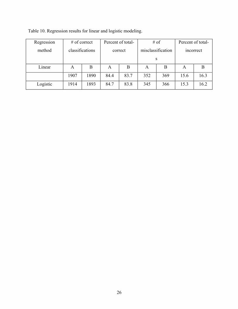
Table 10. Regression results for linear and logistic modeling.

Regression

method

# of correct

classifications

Percent of total-

correct

# of

misclassification

s

Percent of total-

incorrect

Linear A B A B A B A B

1907 1890 84.4 83.7 352 369 15.6 16.3

Logistic 1914 1893 84.7 83.8 345 366 15.3 16.2

26

1a.

0 1000 2000 3000 4000 5000 6000

020

040

060

0

Base (m)

Cas

esNon-tornado

0 1000 2000 3000 4000 5000 6000

020

040

060

0

Base (m)

Cas

es

Tornado

1b. 0 2000 4000 6000 8000 10000 12000

020

040

060

0

Depth (m)

Cas

es

0 2000 4000 6000 8000 10000 12000

020

040

060

0

Depth (m)

Cas

es

1c. 0 5 10 15 20 25

020

040

060

0

S trength rank

Cas

es

0 5 10 15 20 25

020

040

060

0

S trength rank

Cas

es

Figure 1. Histograms of tornado events (panels in left column) versus non-tornado events

(panels in right column) for each of the 23 MDA attributes.

27

1d. 0 5000 10000 15000

020

040

060

0

Low-level diameter (m)

Cas

es

0 5000 10000 15000

020

040

060

0

Low-level diameter (m)

Cas

es

1e. 0 5000 10000 15000

020

040

060

0

Maximum diameter (m)

Cas

es

0 5000 10000 15000

020

040

060

0

Maximum diameter (m)

Cas

es

1f. 0 2000 4000 6000 8000 10000 12000

020

040

060

0

Height of maximum diameter (m)

Cas

es

0 2000 4000 6000 8000 10000 12000

020

040

060

0

Height of maximum diameter (m)

Cas

es

1g. 0 10 20 30 40 50 60

020

040

060

0

Low-level rotational velocity (m/s)

Cas

es

0 10 20 30 40 50 60

020

040

060

0

Low-level rotational velocity (m/s)

Cas

es

Figure 1. Continued.

28

1h. 0 10 20 30 40 50 60

020

040

060

0

Maximum rotational velocity (m/s)

Cas

es

0 10 20 30 40 50 60

020

040

060

0

Maximum rotational velocity (m/s)

Cas

es

1i. 0 2000 4000 6000 8000 10000 12000

020

040

060

0

Height of maximum rotational velocity (m)

Cas

es

0 2000 4000 6000 8000 10000 12000

020

040

060

0

Height of maximum rotational velocity (m)

Cas

es

1j. 0 20 40 60 80 100 120

020

040

060

0

Low-level shear (m/s)

Cas

es

0 20 40 60 80 100 120

020

040

060

0

Low-level shear (m/s)

Cas

es

1k.0 20 40 60 80 100 120

020

040

060

0

Maximum shear (m/s)

Cas

es

0 20 40 60 80 100 120

020

040

060

0

Maximum shear (m/s)

Cas

es

Figure 1. Continued.

29

1l. 0 2000 4000 6000 8000 10000 12000

020

040

060

0

Height of maximum shear (m/s)

Cas

es

0 2000 4000 6000 8000 10000 12000

020

040

060

0

Height of maximum shear (m/s)

Cas

es

1m.0 20 40 60 80 100

020

040

060

0

Low-level gate-to-gate velocity difference (m/s)

Cas

es

0 20 40 60 80 100

020

040

060

0

Low-level gate-to-gate velocity difference (m/s)

Cas

es

1n. 0 20 40 60 80 100

020

040

060

0

Maximum gate-to-gate velocity difference (m/s)

Cas

es

0 20 40 60 80 100

020

040

060

0

Maximum gate-to-gate velocity difference (m/s)

Cas

es

1o. 0 2000 4000 6000 8000 10000 12000

020

040

060

0

Height of maximum gate-to-gate velocity difference (m)

Cas

es

0 2000 4000 6000 8000 10000 12000

020

040

060

0

Height of maximum gate-to-gate velocity difference (m)

Cas

es

. Figure 1. Continued.

30

1p. 0 1000 2000 3000 4000 5000 6000

020

040

060

0

Core base (m)

Cas

es

0 1000 2000 3000 4000 5000 6000

020

040

060

0

Core base (m)

Cas

es

1q. 0 2000 4000 6000 8000

020

040

060

0

Core depth (m)

Cas

es

0 2000 4000 6000 8000

020

040

060

0

Core depth (m)

Cas

es

1r. 0 50 100 150

020

040

060

0

Age (min)

Cas

es

0 50 100 150

020

040

060

0

Age (min)

Cas

es

1s. 0 2000 4000 6000 8000 10000 12000

020

040

060

0

S trength index (M SI) we ighted by average density o f in tegra ted layer

Cas

es

0 2000 4000 6000 8000 10000 12000

020

040

060

0

S trength index (M SI) we ighted by average density o f in tegra ted layer

Cas

es

Figure 1. Continued

31

1t. 0 5 10 15

020

040

060

0

Strength index (MSIr) 'rank'

Cas

es

0 5 10 15

020

040

060

0

Strength index (MSIr) 'rank'

Cas

es

1u. 0 20 40 60 80 100

020

040

060

0

Relative depth (%)

Cas

es

0 20 40 60 80 100

020

040

060

0

Relative depth (%)

Cas

es

1v. 0 10 20 30 40 50 60

020

040

060

0

Low-level convergence (m/s)

Cas

es

0 10 20 30 40 50 60

020

040

060

0

Low-level convergence (m/s)

Cas

es

1w. 0 20 40 60 80 100

020

040

060

0

M id-level convergence (m/s)

Cas

es

0 20 40 60 80 100

020

040

060

0

M id-level convergence (m/s)

Cas

es

Figure 1. Continued.

32

Simple relationships:

Maximum diameter

??

- No correlation

- Three correlations

Base

Low-level convergenceCore base

--

+

- Two correlations

Low-level diameter Low-level shear-

2a.

Height of m aximum GTGVD

Height of m aximum

rotational velocity

Core base

Height of maxim um shear

+

+

+

+

+

- Four correlations

2b.

Figure 2. Different complexities of correlation relationships. Panel a has simple relationships, Panel b has moderate complexity, and Panel c illustrates a highly complex relationship.

33

Low-level rotational velocity

Strength rank Low-level shear

Maximum GTGVD

Strength index “rank”

Strength index

Low-level GTGVD

Maximum rotational velocityAll positive correlations

- 6 or m ore correlations

2c.

Figure 2. Continued.

34

1 2 3 4 5 6 7 8 9 PCs

-1

0

1

2

Scores

Case 38

1 2 3 4 5 6 7 8 9 PCs

-1.0

-0.5

0.0

0.5

1.0

1.5

Scores

Case 59

Figure 3. Individual tornado profiles showing the score on each PC.

35