Analysis of Optimization Experiments

V. ROSHAN JOSEPH∗

Georgia Institute of Technology, Atlanta, GA 30332-0205

and

JAMES DILLON DELANEY†

Carnegie Mellon University, Pittsburgh, PA 15213-3890

Abstract

The typical practice for analyzing industrial experiments is to identify statistically

significant effects with a 5% level of significance and then to optimize the model con-

taining only those effects. In this article, we illustrate the danger in utilizing this

approach. We propose methodology using the practical significance level, which is a

quantity that a practitioner can easily specify. We also propose utilizing empirical

Bayes estimation which gives shrinkage estimates of the effects. Interestingly, the me-

chanics of statistical testing can be viewed as an approximation to empirical Bayes

estimation, but with a significance level in the range of 15-40%. We also establish the

connections that our approach has with a less known but intriguing technique proposed

by Taguchi, known as the beta coefficient method. A real example and simulations are

used to demonstrate the advantages of the proposed methodology.

Key Words: Empirical Bayes method; Practical significance level; Shrinkage estimation;

Variable selection.∗Dr. Joseph is an Assistant Professor in the H. Milton Stewart School of Industrial and Systems Engi-

neering at Georgia Tech. He is a Member of ASQ. His email address is roshan@isye.gatech.edu.†Dr. Delaney is a Visiting Assistant Professor in the Department of Statistics at Carnegie Mellon Uni-

versity. His email address is jdelaney@stat.cmu.edu.

1

Introduction

Experiments are used for many purposes such as for optimizing a process, for developing

a prediction model, for identifying important factors, and for validating a scientific theory.

Among these, optimization is perhaps the most important objective in industrial experiments

(Taguchi 1987, Wu and Hamada 2000, Myers and Montgomery 2002, Montgomery 2004).

However, the same type of data analysis is used irrespective of the underlying objective.

Here we argue that the analysis of optimization experiments should be done in a different

way.

The existing approach to data analysis is to first identify the statistically significant effects

affecting the response. Analysis of variance, t-tests, half-normal plots, step-wise regression,

and other variable selection techniques are used for this purpose. Once the significant effects

are identified, a model is built involving only those effects. The model is then optimized

to find the best settings of the factors. The factors that are not statistically significant are

allowed to take any values in the experimental range. Their settings are left at the discretion

of the experimenter. The usual recommendation is to choose levels that minimize the total

cost. The foregoing might be adequate, but it is in the step of identifying the significant

factors where something can go wrong.

The basic flaw in the methodology is that the objective of optimization cannot be easily

translated into meaningful quantities used in a significance test. An α level of 5% is usually

used for identifying the significant effects. But what is this significance level’s connection to

the optimization of a machining process in order to reduce dimensional variation or the opti-

mization of a chemical process in order to improve yield? Using a quantity in a methodology

that has no direct connection to the objective of the experiment can be misleading.

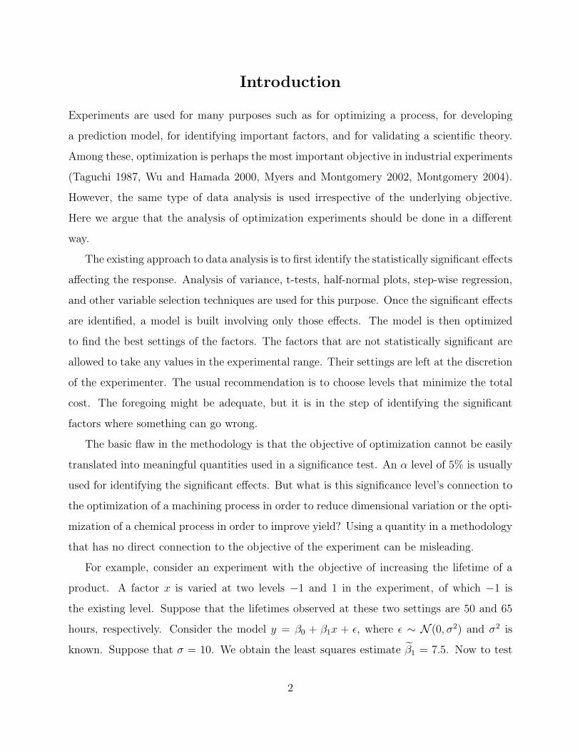
For example, consider an experiment with the objective of increasing the lifetime of a

product. A factor x is varied at two levels −1 and 1 in the experiment, of which −1 is

the existing level. Suppose that the lifetimes observed at these two settings are 50 and 65

hours, respectively. Consider the model y = β0 + β1x + ε, where ε ∼ N (0, σ2) and σ2 is

known. Suppose that σ = 10. We obtain the least squares estimate β1 = 7.5. Now to test

2

the hypothesis H0 : β1 = 0 against H1 : β1 6= 0, we obtain

p-value = 2Φ

(− |β1|

σ/√

2

)= .2888,

where Φ is the standard normal distribution function. This level is much higher than α = .05,

hence we would not reject H0 and might conclude that the factor is not significant.

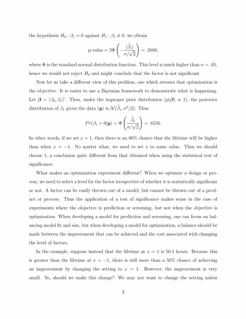
Now let us take a different view of this problem, one which stresses that optimization is

the objective. It is easier to use a Bayesian framework to demonstrate what is happening.

Let β = (β0, β1)′. Then, under the improper prior distribution (p(β) ∝ 1), the posterior

distribution of β1 given the data (y) is N (β1, σ2/2). Thus

Pr(β1 > 0|y) = Φ

(β1

σ/√

2

)= .8556.

In other words, if we set x = 1, then there is an 86% chance that the lifetime will be higher

than when x = −1. No matter what, we need to set x to some value. Thus we should

choose 1, a conclusion quite different from that obtained when using the statistical test of

significance.

What makes an optimization experiment different? When we optimize a design or pro-

cess, we need to select a level for the factor irrespective of whether it is statistically significant

or not. A factor can be easily thrown out of a model, but cannot be thrown out of a prod-

uct or process. Thus the application of a test of significance makes sense in the case of

experiments where the objective is prediction or screening, but not when the objective is

optimization. When developing a model for prediction and screening, one can focus on bal-

ancing model fit and size, but when developing a model for optimization, a balance should be

made between the improvement that can be achieved and the cost associated with changing

the level of factors.

In the example, suppose instead that the lifetime at x = 1 is 50.1 hours. Because this

is greater than the lifetime at x = −1, there is still more than a 50% chance of achieving

an improvement by changing the setting to x = 1. However, the improvement is very

small. So, should we make this change? We may not want to change the setting unless

3

the improvement of .1 hours is worth more to us than the increase in cost of producing the

product with x = 1. Thus if the improvement is practically insignificant, then we may decide

not to make any change. Let ∆ denote the practical significance level. Then a change will

be made if |2β1| > ∆, where β1 is the posterior mean of β1, which in this case is the same as

β1 (note that when x is changed from −1 to 1, the predicted mean response is changed by

2β1). For example, ∆ could be taken to be 5% of the existing lifetime. Thus we will make a

change if the improvement is more than 2.5 hours. Note that here, the use of the 5% level

is much more meaningful than the 5% level used in the test of significance. It is much easier

to say “make a change if it can result in at least a 5% improvement” than to say “make a

change if the factor is statistically significant at the 5% level”. We should note that practical

significance is not a new concept (see, e.g., Montgomery 2004), however, we have not seen

it being used as part of any rigorous methodology.

An objection to this methodology as it is described so far, could be that it does not

consider the randomness in the response (i.e., β1 does not depend on σ2). One approach

to overcome this problem is to compute the probability Pr(|2β1| > ∆|y) and declare x1 as

practically significant when this probability is high enough. However, when more than one

factor is involved in the experiment, the computation of such probabilities becomes difficult.

Therefore, we propose a different approach. We show that empirical Bayes (EB) estimation,

assuming a proper prior distribution for β1, gives an estimate that shrinks as σ increases.

Thus when σ is large enough, the expected improvement is less than ∆, suggesting no change

should be made for that factor setting.

Many authors have advocated using a Bayesian approach for the analysis of experiments.

Box and Meyer (1993) proposed a Bayesian approach to identify active effects from a screen-

ing experiment. See also the follow-up papers by Meyer et al. (1996) and Chipman et al.

(1997). Even though model selection is made less ambiguous than what is encountered in the

usual statistical testing approach, this work does not account for the optimization objective

of an experiment. Peterson (2004) proposed a Bayesian approach when the objective of the

experiment is optimization. His approach is to find the settings of the factors that maximize

the probability that the predicted response is within some desirable range. This approach

4

incorporates the uncertainty in the model parameters through the calculation of the poste-

rior predictive density of the response (see also Miro-Quesada et al. 2004). Rajagopal and

Del Castillo (2005) proposed an extension of this approach that also takes into account the

uncertainty of the model form. This is achieved by obtaining the posterior predictive distri-

bution averaged over a candidate class of models. One major difference between their work

and what we propose here is that we try to balance the optimization objective with the cost

of implementing particular factor settings through the introduction of practical significance

levels. However, whereas Rajagopal and Del Castillo (2005) does, we do not incorporate the

model uncertainty. Moreover, because we use an empirical Bayes approach the uncertainty

associated with hyper-parameters is also lost. Nevertheless, our approach leads to a proce-

dure that is very close to the statistical testing procedure, which should readily appeal to

practitioners. In fact, we show that the model selection in a version of our approach can be

approximated by a statistical testing procedure with a higher than typically used significance

level in the range of 15-40%.

The details of the proposed methodology for optimization experiments are described in

the following sections. As discussed before, it differs from the existing approach mainly in

the use of two concepts: practical significance level and EB estimation. First, we present a

real experiment to serve as motivation for adoption of this methodology.

An Example

Consider the experiment reported by Hellstrand (1989) with the objective of reducing the

failure rate of deep groove ball bearings (see also Box et al. 2005, pp. 209–211). A two-

level full factorial design over three factors: osculation (x1), heat treatment (x2), and cage

design (x3), was used for the experiment. The osculation refers to the ratio between the ball

diameter and the radius of the outer ring of the bearing. The response is failure rate (y),

which is defined as the reciprocal of the average time to failure (in hours) × 100. The design

and the data are given in Table 1.

The estimates of the seven effects are given in Table 2. Because this is an unreplicated

5

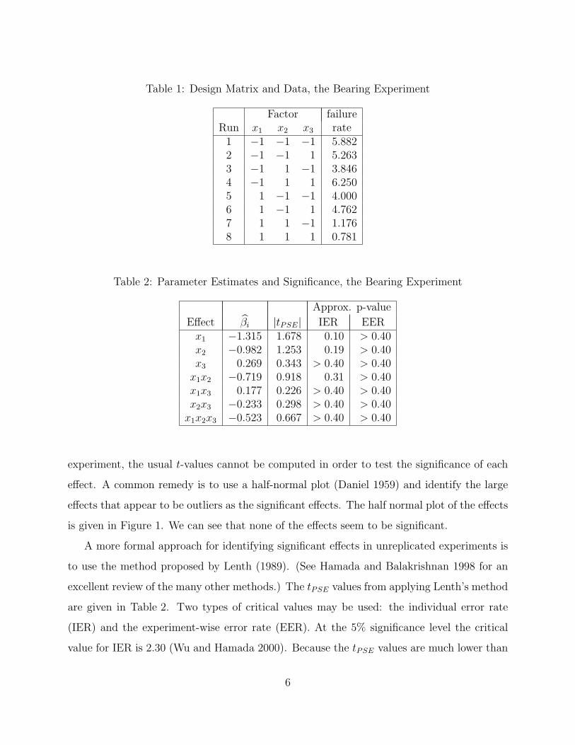
Table 1: Design Matrix and Data, the Bearing Experiment

Factor failureRun x1 x2 x3 rate

1 −1 −1 −1 5.8822 −1 −1 1 5.2633 −1 1 −1 3.8464 −1 1 1 6.2505 1 −1 −1 4.0006 1 −1 1 4.7627 1 1 −1 1.1768 1 1 1 0.781

Table 2: Parameter Estimates and Significance, the Bearing Experiment

Approx. p-value

Effect βi |tPSE| IER EERx1 −1.315 1.678 0.10 > 0.40x2 −0.982 1.253 0.19 > 0.40x3 0.269 0.343 > 0.40 > 0.40

x1x2 −0.719 0.918 0.31 > 0.40x1x3 0.177 0.226 > 0.40 > 0.40x2x3 −0.233 0.298 > 0.40 > 0.40

x1x2x3 −0.523 0.667 > 0.40 > 0.40

experiment, the usual t-values cannot be computed in order to test the significance of each

effect. A common remedy is to use a half-normal plot (Daniel 1959) and identify the large

effects that appear to be outliers as the significant effects. The half normal plot of the effects

is given in Figure 1. We can see that none of the effects seem to be significant.

A more formal approach for identifying significant effects in unreplicated experiments is

to use the method proposed by Lenth (1989). (See Hamada and Balakrishnan 1998 for an

excellent review of the many other methods.) The tPSE values from applying Lenth’s method

are given in Table 2. Two types of critical values may be used: the individual error rate

(IER) and the experiment-wise error rate (EER). At the 5% significance level the critical

value for IER is 2.30 (Wu and Hamada 2000). Because the tPSE values are much lower than

6

0.0 0.5 1.0 1.5

0.2

0.4

0.6

0.8

1.0

1.2

half−normal quantiles

| ββ |

x3

x2x3x1x2

x1x3

x1x2x3

x2

x1

Figure 1: Half Normal Plot for the Bearing Experiment

this value, none of the effects are found to be significant. The EER critical value is 4.87,

which is much larger than the IER critical value, and thus the same conclusion would be

obtained. We can also compute the p-values for each effect based on IER and EER. They

are also shown in Table 2. We can see that the p-values are large enough to conclude that

none of the effects are significant.

By examining the data in Table 1, we can see that run numbers 7 and 8 produce failure

rates that are much lower than those of the other runs. It appears that keeping osculation

and temperature both at their high values is beneficial. Hellstrand (1989) identified this

setting using simple interaction plots. He confirmed this choice of factor settings through

observing vastly improved bearing performance in its subsequent use. These settings yielded

a substantial improvement in failure rate that would have been missed if we were to rely

upon only the statistical test of significance.

7

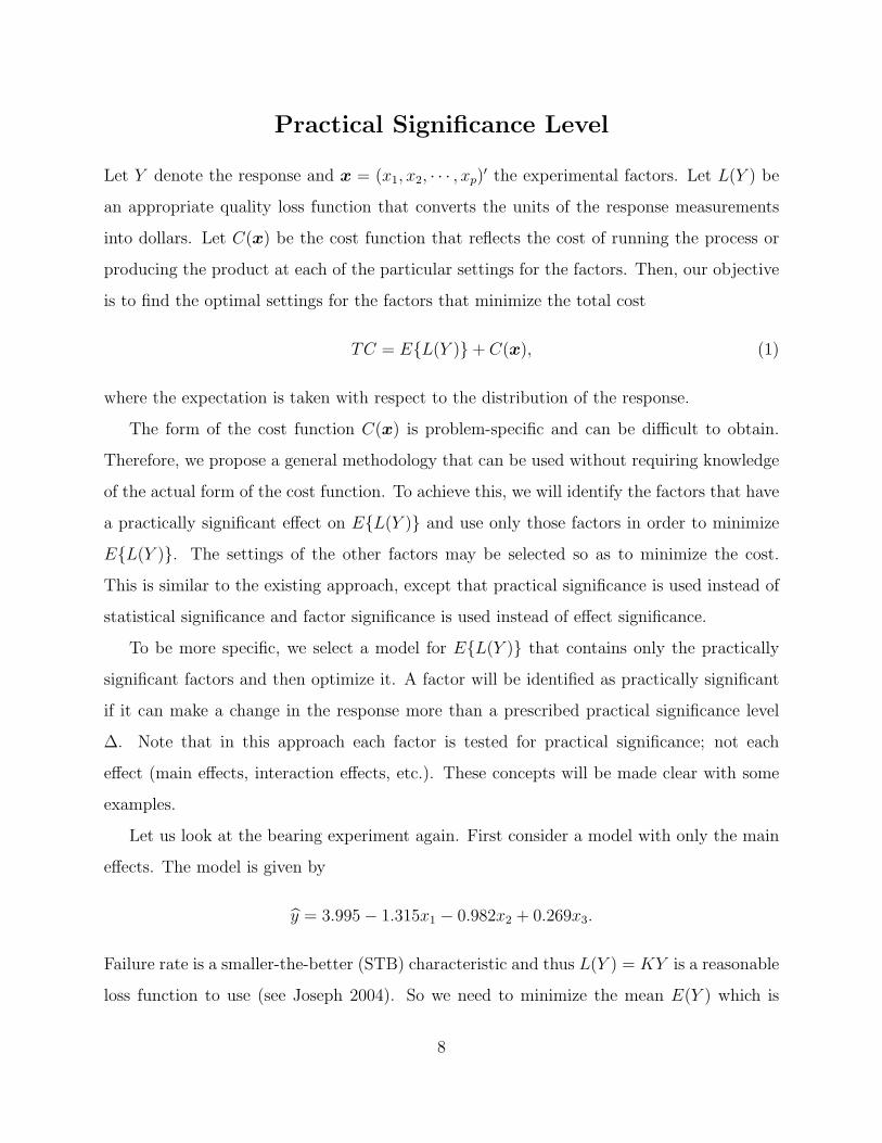
Practical Significance Level

Let Y denote the response and x = (x1, x2, · · · , xp)′ the experimental factors. Let L(Y ) be

an appropriate quality loss function that converts the units of the response measurements

into dollars. Let C(x) be the cost function that reflects the cost of running the process or

producing the product at each of the particular settings for the factors. Then, our objective

is to find the optimal settings for the factors that minimize the total cost

TC = E{L(Y )}+ C(x), (1)

where the expectation is taken with respect to the distribution of the response.

The form of the cost function C(x) is problem-specific and can be difficult to obtain.

Therefore, we propose a general methodology that can be used without requiring knowledge

of the actual form of the cost function. To achieve this, we will identify the factors that have

a practically significant effect on E{L(Y )} and use only those factors in order to minimize

E{L(Y )}. The settings of the other factors may be selected so as to minimize the cost.

This is similar to the existing approach, except that practical significance is used instead of

statistical significance and factor significance is used instead of effect significance.

To be more specific, we select a model for E{L(Y )} that contains only the practically

significant factors and then optimize it. A factor will be identified as practically significant

if it can make a change in the response more than a prescribed practical significance level

∆. Note that in this approach each factor is tested for practical significance; not each

effect (main effects, interaction effects, etc.). These concepts will be made clear with some

examples.

Let us look at the bearing experiment again. First consider a model with only the main

effects. The model is given by

y = 3.995− 1.315x1 − 0.982x2 + 0.269x3.

Failure rate is a smaller-the-better (STB) characteristic and thus L(Y ) = KY is a reasonable

loss function to use (see Joseph 2004). So we need to minimize the mean E(Y ) which is

8

estimated by y. Suppose that the existing level of failure rate is 5 and a 5% decrease is

considered to be a significant improvement, then we can take ∆ = .05×5 = .25. Each of the

factors can independently make a change of two times its coefficient estimate (because they

vary from −1 to 1). All of these are more than .25 and so all of the factors are identified as

practically significant, a very different conclusion from that arrived at from the application

of the statistical significance level.

We note that the expected loss function in the foregoing formulation should be replaced

with other measures of interest, if they are more meaningful to the problem at hand. For

example, if the quality characteristic is of the nominal-the-best variety, we may perform the

analysis on the mean and variance separately; if the quality characteristic is of the larger-

the-better variety, we may perform the analysis on the mean; and so on. It is important

to choose a measure that is readily understandable by the experimenter, so that ∆ can be

easily chosen.

Now consider the full linear model with interactions,

y = 3.995−1.315x1−0.982x2+0.269x3−0.719x1x2−0.177x1x3+0.233x2x3−0.523x1x2x3. (2)

In statistical hypothesis testing, the magnitudes of all seven effects are tested for their

significance. In that setting, there is a penalty associated with including each effect in the

model. In the proposed methodology only the significance of a factor is considered. There

is no penalty for including an interaction effect when their parent effects are already in the

model, because we only consider the cost associated with each factor, not with each effect.

This is more reasonable when optimization is the objective.

To apply the practical significance level to each factor, we would need to know the effect

of each factor. But then since interactions are present, the effect of a factor changes with the

settings of the other factors. When there are factors present that have more than two levels,

we might consider their quadratic, cubic, etc. effects. Therefore, we need a more general

concept than “effects”. To address this issue and alleviate any confusion with the definition

of factorial effects, we introduce the concept of the impact of a factor with respect to the

optimal setting of x.

9

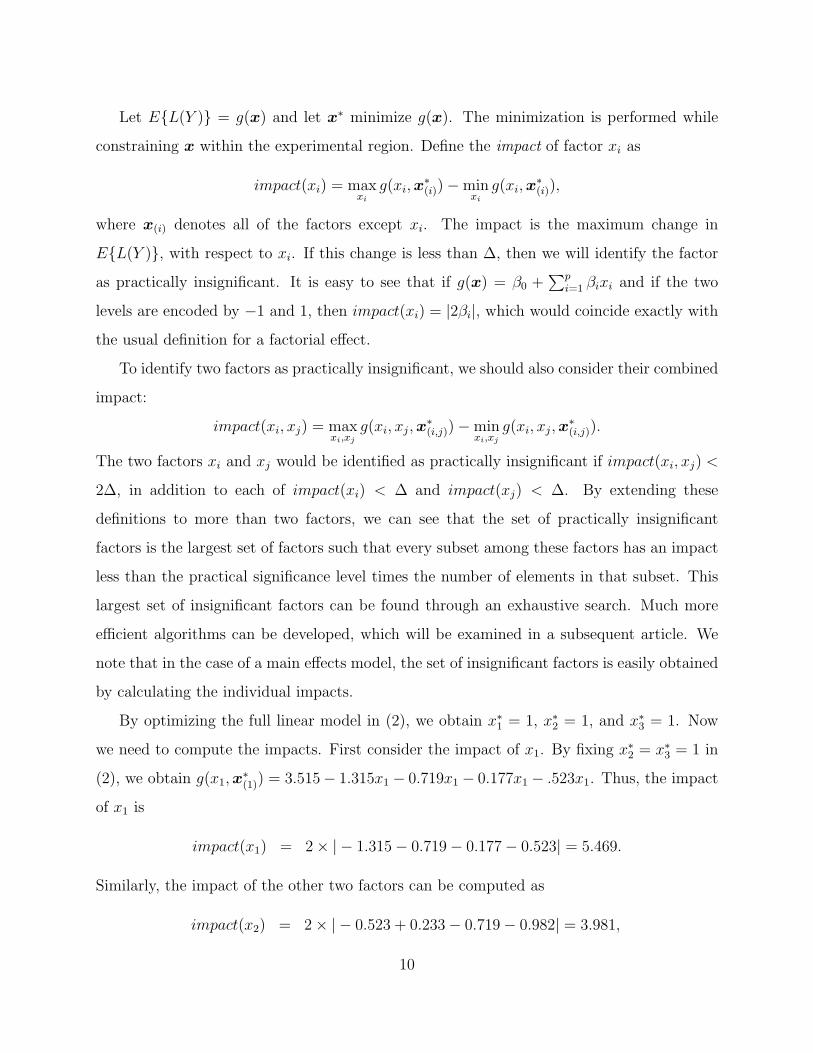
Let E{L(Y )} = g(x) and let x∗ minimize g(x). The minimization is performed while

constraining x within the experimental region. Define the impact of factor xi as

impact(xi) = maxxi

g(xi, x∗(i))−min

xi

g(xi, x∗(i)),

where x(i) denotes all of the factors except xi. The impact is the maximum change in

E{L(Y )}, with respect to xi. If this change is less than ∆, then we will identify the factor

as practically insignificant. It is easy to see that if g(x) = β0 +∑p

i=1 βixi and if the two

levels are encoded by −1 and 1, then impact(xi) = |2βi|, which would coincide exactly with

the usual definition for a factorial effect.

To identify two factors as practically insignificant, we should also consider their combined

impact:

impact(xi, xj) = maxxi,xj

g(xi, xj, x∗(i,j))−min

xi,xj

g(xi, xj, x∗(i,j)).

The two factors xi and xj would be identified as practically insignificant if impact(xi, xj) <

2∆, in addition to each of impact(xi) < ∆ and impact(xj) < ∆. By extending these

definitions to more than two factors, we can see that the set of practically insignificant

factors is the largest set of factors such that every subset among these factors has an impact

less than the practical significance level times the number of elements in that subset. This

largest set of insignificant factors can be found through an exhaustive search. Much more

efficient algorithms can be developed, which will be examined in a subsequent article. We

note that in the case of a main effects model, the set of insignificant factors is easily obtained

by calculating the individual impacts.

By optimizing the full linear model in (2), we obtain x∗1 = 1, x∗2 = 1, and x∗3 = 1. Now

we need to compute the impacts. First consider the impact of x1. By fixing x∗2 = x∗3 = 1 in

(2), we obtain g(x1, x∗(1)) = 3.515− 1.315x1 − 0.719x1 − 0.177x1 − .523x1. Thus, the impact

of x1 is

impact(x1) = 2× | − 1.315− 0.719− 0.177− 0.523| = 5.469.

Similarly, the impact of the other two factors can be computed as

impact(x2) = 2× | − 0.523 + 0.233− 0.719− 0.982| = 3.981,

10

impact(x3) = 2× | − 0.523 + 0.233 + 0.269− 0.177| = 0.395.

Because all of these impacts are more than .25, they are all identified as practically significant.

Thus all three factors should be changed to their higher levels so as to minimize the failure

rate. This is a much different conclusion than what we obtain using the statistical significance

tests.

This result is consistent with the conclusion of Hellstrand (1989), except therein the

factor cage design (x3) was not considered significant. Can the observed effect of x3 be due

merely to random error? Are we unnecessarily incurring a potential cost by forcing the cage

design to its higher level? We will answer these questions in the next section.

Empirical Bayes Estimation

Suppose that the response is related to the factors through the model Y = β0 +∑

i βiui + ε,

where ε ∼ N (0, σ2) and ui’s are functions of the factors. For example, in a 23 design we can

take u1 = x1, u2 = x2, u3 = x3, u4 = x1x2, u5 = x1x3, u6 = x2x3, and u7 = x1x2x3. Assume

that σ2 is known. If unknown, it can be estimated from replicates. Let u = (1, u1, u2, · · ·)′ and

β = (β0, β1, β2, · · ·)′. Then Y = u′β+ε. In a Bayesian framework, we would need to specify a

prior distribution for β. For notational simplicity, rewrite the model as Y = µ+u′β+ε, where

µ denotes the prior mean for β0. We assume the multivariate normal prior: β ∼ N (0,Σ).

Let the design have n runs and let U be the corresponding model matrix. Let y denote

the data obtained from the experiment. Assuming the ε’s are independent, we have the

Bayesian model

y|β ∼ N (µ1 + Uβ, σ2I) and β ∼ N (0,Σ),

where 1 is a vector of 1’s having length n and I is the n-dimensional identity matrix. Then

the posterior mean of β given the data is

β = ΣU ′(UΣU ′ + σ2I)−1(y − µ1). (3)

The unknown hyper-parameters (i.e., parameters in the prior distribution) can be estimated

using empirical Bayes (EB) methods (see e.g. Carlin and Louis 2000). One common approach

11

to implementing the EB method is to use maximum likelihood estimation of the hyper-

parameters using the marginal distribution of the response. The marginal distribution of

y can be obtained by integrating out β. We obtain y ∼ N (µ1, UΣU ′ + σ2I). Thus, the

log-likelihood of the marginal distribution of y is given by

l = constant− 1

2log det(UΣU ′ + σ2I)− 1

2(y − µ1)′(UΣU ′ + σ2I)−1(y − µ1).

The log-likelihood can be maximized with respect to µ, and the parameters in Σ to obtain

their estimates.

The approach is very general. It can be applied to any type of designs: regular, nonreg-

ular, orthogonal, nonorthogonal, and mixed-level designs. The only condition required for

the existence of EB estimates is that the matrix UΣU ′ + σ2I be nonsingular.

When U is orthogonal and Σ is diagonal some simplifications can be observed. Below

we consider three special structures for Σ. They are presented in the order of increasing

complexity. The last covariance structure is the most preferred, however the discussion of

the first two is provided because it reveals interesting insights into the overall approach.

Before proceeding further, we should mention a disadvantage of using EB methods. In

the EB method the uncertainty due to the hyper-parameter estimation is not accounted for

(see Berger 1985). We can overcome this problem by using a hierarchical Bayes approach,

where a second stage prior is postulated for the hyper-parameters. However, this comes at

the expense of increased computation. In this article we focus on EB methods and leave

further comparisons with the hierarchical Bayes methods for future research.

Identical Variances Prior

Consider the bearing experiment again. Assume that Σ = τ 2I. Because Table 1 reflects a

full factorial design, the columns of U are orthogonal. Thus UΣU ′ = 8τ 2I. From (3), we

obtain

β =U ′(y − µ1)

8 + σ2/τ 2.

12

The least squares estimate of β is given by

β = (U ′U )−1U ′(y − µ1) =1

8U ′(y − µ1).

Thus

β =8

8 + σ2/τ 2β,

which illustrates that the EB estimate shrinks the least squares estimate by the factor 8/(8+

σ2/τ 2).

The marginal log-likelihood simplifies to

l = constant− 8

2log(8τ 2 + σ2)− (y − µ1)′(y − µ1)

2(8τ 2 + σ2).

Differentiating with respect to µ and τ 2 and equating to 0, we obtain the familiar solutions

µ = y

and

8τ 2 + σ2 =1

8

8∑i=1

(yi − y)2.

Denote the right side of this equation, the sample variance of Y , by s2. Then, because τ 2

cannot be negative, we obtain

τ 2 =1

8

(s2 − σ2

)+

,

where (x)+ = x if x > 0 and 0 otherwise. Thus

β =

(1− σ2

s2

)+

β. (4)

Thus the EB estimate of β decreases as σ2 increases and becomes 0 when σ2 exceeds the

observed variance of Y . The above estimator may be recognized as the well-known positive-

part James-Stein estimator (see Lehmann and Casella 1998, pg. 275). The connection

between James-Stein estimation and EB estimation is well-known in the statistical literature.

However, we have not seen it advanced as an alternative to statistical testing in the analysis

of experiments. Note that if replicates are available, then σ2 can be estimated based on the

13

0 1 2 3 4 5

−1.

5−

1.0

−0.

50.

00.

5(a)

σσ2

ββ ββ1

ββ2

ββ3

ββ12

ββ13

ββ23

ββ123

0 1 2 3 4 5

01

23

45

6

(b)

σσ2

Impa

ct

x1

x2

x3

Figure 2: Bearing Experiment With Equal Prior Variances: (a) Coefficients (b) Impacts

sample variance of the replicates. If replicates are not available, then a reasonable guess

value should be used.

The coefficients β1, β2, · · · , β7 are plotted in Figure 2(a) against σ2 (note that β0 = 0).

We can see that as σ2 increases, the β’s decrease to 0. The impacts of the three factors

can be calculated as before and are plotted in Figure 2(b). We can see that the impact of

x3 is practically insignificant at the 5% level (∆ = .25) when σ2 > 1.4. Therefore, if σ2 is

as large as 1.4, then x3 can be set to minimize the cost. This is exactly the same result

obtained by Hellstrand (1989) with his subsequent experiments. The analysis shows that

even in the presence of large random error, the two factors, osculation and heat treatment,

have significant effects and can be adjusted to improve the failure rate substantially. This is

a conclusion completely different from that obtained using the statistical tests of significance.

14

Unequal Variances Prior

Now consider a more general form for Σ. As before, let the βi’s be independent but with

possibly different prior variances: τ 2i . Then Σ = diag(τ 2

0 , τ 21 , · · · , τ 2

7 ). From (3), we obtain

βi =8τ 2

i

8τ 2i + σ2

βi,

and the marginal log-likelihood becomes

l = constant− 1

2

7∑i=0

log(8τ 2i + σ2)− 1

2

7∑i=0

8βi

2

8τ 2i + σ2

. (5)

Minimizing l, we obtain τ 2i = (βi

2− σ2/8)+. Let

zi =βi

σβi

,

which is the usual test statistic for testing H0 : βi = 0 where σβidenotes the standard error

of βi. Because σβi= σ/

√8, we obtain

βi =

(1− 1

z2i

)+

βi. (6)

This shows that βi shrinks completely to 0 if |zi| ≤ 1. This threshold is equivalent to using

α = 31.73% in statistical testing. That is, when |zi| > 1, the ith coefficient is identified as

statistically significant at the 31.73% level and βi is used in the model. Whereas with EB

estimation, a value smaller than βi is used and as |zi| decreases, βi decreases continuously

from βi to zero.

The estimates of the coefficients are plotted in Figure 3(a). In addition, the impacts for

the three factors at their optimal settings are plotted in Figure 3(b). We can see that the

coefficients shrink to 0 at a slower rate. The impact of x3 is practically insignificant at the

5% level (∆ = .25) when σ2 > 1.7. The impacts of x1 and x2 are practically significant,

provided σ2 < 12.5 and σ2 < 6.7, respectively. Note that in this example, we do not have

an estimate of σ2. An engineer working in the deep groove ball bearing process can possibly

give a reasonable estimate. But we can argue that σ2 should be much less than 6.7, because

15

the sample variance of the observed failure rates is only 3.6. Thus our analysis strongly

supports the conclusion that at least x1 and x2 are practically significant.

Although we used the 23 design to derive (6), the result is much more general. It can be

applied to fractional factorial designs (regular and nonregular) and to designs with factors

having more than two levels. The only restriction is that the model matrix corresponding to

the effects that we are trying to estimate should be orthogonal. The proposition is formally

stated below and is proved in the Appendix.

Proposition 1. Let

y = µ1n + Uβ + ε, ε ∼ N (0, σ2In)

and

β ∼ N (0,Σ), where Σ = diag(τ 20 , . . . , τ 2

s−1).

U is an n× s matrix such that U ′U = nIs. Then the EB estimate is

βi = (1− 1

z2i

)+βi,

where β = (U ′U )−1U ′y, the ordinary least squares estimate of β and zi is the test statistic

for testing H0 : βi = 0 vs. H1 : βi 6= 0 with σ2 known, that is zi = βi

σ/√

n.

The methodology can easily be extended to the case of an unknown σ. If an estimate of

σ can be obtained from replicates, then

ti = βi/σβi(7)

has a t distribution with the appropriate degrees of freedom. Thus, the EB estimate in (6)

becomes

βi =

(1− 1

t2i

)+

βi. (8)

Similarly, the estimator in (4) is approximately β = (1 − 1/F )+β, where F is the usual

F -statistic for the overall test of significance (i.e., testing none of the effects are significant

against at least one of them is significant). Thus, when the identical variances prior is

16

0 5 10 15 20

−1.

5−

1.0

−0.

50.

00.

5(a)

σσ2

ββ ββ1

ββ2

ββ3

ββ12

ββ13

ββ23

ββ123

0 5 10 15 20

01

23

45

6

(b)

σσ2

Impa

ct

x1

x2

x3

Figure 3: Bearing Experiment With Unequal Prior Variances: (a) Coefficients (b) Impacts

used, the shrinkage factor depends on the overall F -test statistic, whereas when the unequal

variances prior is used, there are many shrinkage factors, each depending on the individual

t-test statistics.

Heredity Prior

As it is described so far, the methodology does not incorporate the principles of effect

hierarchy and effect heredity (Hamada and Wu 1992). Because the main effects, two-factor

interactions, and the three-factor interaction are all treated the same way, effect hierarchy

is not reflected in the methodology. Because an interaction term can appear in the model

without any of its parent factors, effect heredity is also not reflected in the methodology. We

can remedy this. Joseph (2006) and Joseph and Delaney (2007) show that these principles

can easily be incorporated into the analysis through the prior specification. Let Σ = τ 2R,

where R = diag(1, r1, r2, r3, r1r2, r1r3, r2r3, r1r2r3), and ri ∈ [0, 1] for all i. Then, from (3),

17

0 2 4 6 8 10

−1.

5−

1.0

−0.

50.

00.

5(a)

σσ2

ββ ββ1

ββ2

ββ3

ββ12

ββ13

ββ23

ββ123

0 2 4 6 8 10

01

23

45

6

(b)

σσ2

Impa

ct

x1

x2

x3

Figure 4: Bearing Experiment With Heredity Prior: (a) Coefficients (b) Impacts

we obtain

βi =8τ 2Rii

8τ 2Rii + σ2βi,

where Rii represents the (i + 1)th diagonal element of R. Furthermore, the marginal log-

likelihood becomes

l = constant− 1

2

7∑i=0

log(8τ 2Rii + σ2

)− 1

2

7∑i=0

8βi

2

8τ 2Rii + σ2. (9)

We may numerically maximize this log-likelihood in order to find the EB estimates for the

hyper-parameters µ, r1, r2, r3, and τ 2.

The consequence of assuming the heredity prior can readily be discerned from the plot of

the coefficients that is given in Figure 4(a). Coefficients are zeroed in groups as σ2 increases.

For instance, both β2 and the interaction β1,2 are zero for all σ2 > 6. The separation

between the significant factors and insignificant factors is quite discernable. For σ2 < 6.3,

x1 is practically significant, for σ2 < 5.5, x2 is practically significant, and for σ2 < 0.3, x3 is

practically significant. That is, the factor x3, cage design, is practically insignificant under

18

virtually all assumptions for the error variance. The impacts in Figure 4(b) are once again

consistent with the conclusion of Hellstrand (1989).

Shrinkage Estimation Methods

Taguchi (1987, chapter 19) criticized the use of statistical testing in experiments and pro-

posed an intriguing method which he named the beta coefficient method. He notes on page

566 of his book that “when results obtained by experiment are actually applied, it is rare

that an effect greater than the experimental results is obtained, and that in most cases less

than the expected effect is obtained.” Therefore, he suggested that the effects obtained from

an experiment should be shrunk towards 0 before making the prediction. Taguchi denoted

the shrinkage factor by the parameter β and so he named the method the beta coefficient

method. But because the variable β is more commonly used for denoting the linear model

parameters, we introduce different notation, λ.

Taguchi developed his method using an analysis of variance model and the sum of squares

calculations, but for the consistency of exposition, we explain his method using the regression

model set up that is used throughout this article. Let λi denote the shrinkage factor applied

to the least squares estimate βi. The objective is to find the λi that minimizes the mean

squared error E{(λiβi − βi)2}. Because E(βi) = βi, we obtain

E{(λiβi − βi)2} = λ2

i var(βi) + (1− λi)2β2

i .

Differentiating with respect to λi and equating to 0, we obtain

λi =β2

i

β2i + var(βi)

= 1− var(βi)

β2i + var(βi)

.

If the columns in the model matrix are orthogonal, then var(βi) = σ2/n. An unbiased

estimate of β2i + σ2/n is β2

i . Thus λi can be estimated by

λi = 1− σ2/n

β2i

= 1− 1

t2i. (10)

19

Because λi must be nonnegative, modifying the estimate to λi = (1 − 1/t2i )+ is required.

This produces the shrinkage coefficient suggested by Taguchi. This is exactly the same as

the EB estimate in (8).

Although the EB approach (with unequal variances prior) leads to the same approach

suggested by Taguchi, we note that the EB perspective admits an even more general proce-

dure that can be used with any type of design (it need not be orthogonal) and that easily

incorporates effect hierarchy and heredity. This should lead to better models and better

decision making.

The value of using shrinkage estimation for improving efficiency is evident from its pres-

ence in the statistical literature (Gruber 1998). Recently, there has been a surge of interest in

developing methods that are a combination of shrinkage and subset selection. These meth-

ods include the nonnegative (nn) garrote by Breiman (1995), the least absolute shrinkage

and selection operator (lasso) by Tibshirani (1996), and least angle regression (LARS) by

Efron et al. (2004). EB estimation has connections to the nn-garrote, which can be seen

by considering orthogonal designs. Breiman (1995) showed that the estimate of βi in the

nn-garrote scheme is given by

βi =

(1− c

β2i

)+

βi,

where βi is the least squares estimate and c is estimated from the data using cross validation

methods. If we replace c with σ2/n, then the nn-garrote estimator is exactly the same as

the one we obtained in (8). However, the EB estimate is more general than the nn-garrote

estimate. This is because, in fractional factorial designs the number of effects to estimate

is more than the number of runs, in which case least squares estimates do not exist. Thus,

the nn-garrote estimates also do not exist, whereas the EB estimates can still be found (see

Joseph 2006 and Joseph and Delaney 2007).

20

Statistical Testing as an Approximation

For the EB estimate in (6), the value of βi in the estimated model can be expressed: λiβi,

where λi = (1− 1/z2i )+. In statistical hypothesis testing, λi = 0 when |zi| ≤ zα/2 and λi = 1

otherwise. As discussed in the introduction, it is difficult to find a meaningful statistical

significance level, α, for a given problem. However, the similarity of this testing procedure

with the EB estimation reveals that statistical testing can be used as an approximation.

A simple approximation is to take zα/2 = 1, which yields α = 31.73%. But because the

EB estimates shrink towards 0 when zi > 1, we may prefer to search for an even closer

approximate statistical test.

A plot of λ as a function of z is provided in Figure 5(a). The objective is to find the zα/2

that minimizes the absolute difference between the EB estimate and the estimate implicit in

statistical testing. Under the null hypothesis, z ∼ N (0, 1). Thus, we minimize∫ zα/2

1

{(1− 1

z2)− 0}φ(z) dz +

∫ ∞

zα/2

{1− (1− 1

z2)}φ(z) dz,

where φ(z) is the standard normal density function. By differentiating with respect to zα/2

and equating to 0, we obtain

(1− 1

z2α/2

)φ(zα/2)−1

z2α/2

φ(zα/2) = 0.

Solving, we obtain zα/2 =√

2. This corresponds to α = 15.73%. At this level, the EB

estimate of βi is one half of the least squares estimate.

Because of the popularity of statistical testing and its primacy in the analysis techniques

described in many textbooks on the design and analysis of experiments, we envision that

it will continue to be used for many more years to come. Moreover, the procedure using

statistical testing is easier to implement than EB estimation. So if an investigator prefers

to apply statistical testing, we recommend using α = 15%. Taguchi (1987) also noted that

statistical testing is acceptable as a procedure as long as it is viewed as an approximation

to his beta coefficient method. However, he did not suggest any optimal value for α as we

did here.

21

−3 −2 −1 0 1 2 3

0.0

0.2

0.4

0.6

0.8

1.0

(a)

z

λλ

−− 2 2 0 5 10 15 20 25 30

0.0

0.1

0.2

0.3

0.4

0.5

(b)

νν

αα

Figure 5: Testing as an Approximation: (a) Shrinkage as a Function of Critical Values:

Hypothesis Testing (dashed), EB Estimation (solid), (b) Optimal significance levels for t-

tests

Note that the significance level α is the probability of mistakenly declaring a given effect

as nonzero. When many effects are tested simultaneously, the probability of mistakenly

declaring at least one effect as nonzero will be larger than α. To overcome this problem,

multiple testing methods such as the Bonferronni correction method and the studentized

maximum modulus method are recommended in the literature (see, e.g. Wu and Hamada

2000). However, our derivation demonstrates that α = .15 should be used irrespective of the

number of effects being examined. Therefore, in optimization experiments, we recommend

against using multiple testing procedures.

If σ can be estimated, then a t-statistic could be used for testing H0: βi = 0. Note

that the optimal critical value is still√

2, irrespective of the distribution of the test statistic.

Therefore, the optimal significance level in a t-test can be obtained by solving for α in

tα/2,ν =√

2, where ν represents the degrees of freedom for the error. For ν = 1, we obtain

α = .3918. This approaches .1573 as ν →∞ (see Figure 5(b)).

22

It is a common practice to use a higher significance level when stepwise regression meth-

ods are applied for variable selection. In this setting, Kennedy and Bancroft (1971) offer

simulation results to suggest using a statistical significance level in the range of .10 to .25.

Our theoretical results provide further justification for this choice. Moreover, a different level

of α would be associated with different degrees of freedom. In fact, it is better to fix the

t-critical value at√

2 instead of specifying any particular α-level. Most statistical software

use an F -critical value for entering or removing a variable from the model. This critical

value should be set at (√

2)2 = 2.

Simulation

We use simulation to investigate the properties of the proposed methodology for optimization

experiments. Below, we consider the estimation of the main effects from a design that is a

12-run orthogonal array over 11 factors, with the model matrix (see, e.g. Wu and Hamada

2000):

U =

1 1 1 −1 1 1 1 −1 −1 −1 1 −11 −1 1 1 −1 1 1 1 −1 −1 −1 11 1 −1 1 1 −1 1 1 1 −1 −1 −11 −1 1 −1 1 1 −1 1 1 1 −1 −11 −1 −1 1 −1 1 1 −1 1 1 1 −11 −1 −1 −1 1 −1 1 1 −1 1 1 11 1 −1 −1 −1 1 −1 1 1 −1 1 11 1 1 −1 −1 −1 1 −1 1 1 −1 11 1 1 1 −1 −1 −1 1 −1 1 1 −11 −1 1 1 1 −1 −1 −1 1 −1 1 11 1 −1 1 1 1 −1 −1 −1 1 −1 11 −1 −1 −1 −1 −1 −1 −1 −1 −1 −1 −1

.

Models were simulated with the following mechanism:

f(βi|ηi) = ηiN (0, τ 2) + (1− ηi)N (0, 1) i = 0, . . . , 11

ηi =

1 with probability 1− γ

0 with probability γ.

23

Y = µ + Uβ + ε ε ∼ N (0, σ2).

Similar models are widely used in the analysis of experiments (see, e.g., Chipman et al.

1997). ηi is an indicator variable that controls whether effect i is active or inactive. This

happens with probability γ and 1 − γ respectively. When the effect is active (ηi = 0), the

coefficient is drawn from N (0, 1) and when it is inactive (ηi = 1), the coefficient is drawn

from N (0, τ 2), where τ 2 << 1. By making τ 2 small, we ensure that the inactive effects are

small.

Without loss of generality, we assume µ = 0. First consider the case when σ2 is known.

Then, for each of these models we carry out estimation and variable selection in the tra-

ditional frequentist manner, using statistical hypothesis testing. The significance levels of

α = .0045, α = .0500, and α = .1573 respectively correspond to: the Bonferroni adjustment

to α = .05 to properly account for simultaneous testing, the α-level required for declaring

significance in many publications, and the level we recommend as an approximation to the

EB procedure as discussed above, respectively. The hypothesis test corresponding to these

levels will be applied to the standard least squares parameter estimates. For EB estimation,

we use (6) or (8) depending on whether σ2 is known or unknown. In addition, results are

presented for a variety of levels of the practical significance level (∆) applied to the EB es-

timates, so as to identify up to 11 factor impacts. N=10,000 random models were generated

for many different values for σ2, τ 2, and γ.

We assume that Y is a larger-the-better quality characteristic. For each simulation j, we

have a true model for the response yj(x). Let x† represent the true optimal factor settings.

Then yj(x†) =

∑11i=1 |β

(j)i |, where β

(j)i is the coefficient of xi in the jth model. For simplicity,

assume that the existing setting is 0 for all of the factors. Thus yj(0) = 0. Therefore yj(x†)

can be viewed as the improvement obtained in an experiment with the jth true model.

Thus the average improvement is 1/N∑N

i=1 yj(x†). Let x∗ denotes the factor settings we

would choose when employing an estimation and thresholding methodology. The average

improvement with that methodology is 1/N∑N

i=1 yj(x∗). Thus the percent improvement can

24

be calculated by

% Improvement =

∑Nj=1 yj(x

∗)∑Nj=1 yj(x†)

× 100.

Because our objective in an optimization experiment is to balance quality with cost, we need

a metric to asses the cost. In a main effects model, the cost might be considered to be

proportional to the number of active effects. Therefore, we use the average number of active

effects as a second metric to evaluate the performance of different techniques. Therefore, a

good methodology should yield high values for the % Improvement and low values for the

Number of Active Effects.

Table 3: Simulation results (γ = 0.5, τ 2 = 0.001, σ2 known)

% ImprovementStatistical Significance (α) Practical Significance (∆)

σ2 0.0045 0.0500 0.1573 0.0 0.1 0.2 0.3 0.4 0.50.0 100 100 100 100 98 96 96 95 940.5 81 88 91 93 93 92 91 90 891.0 68 80 86 90 89 88 87 87 852.0 51 68 78 84 83 82 81 80 795.0 25 47 61 70 70 69 68 67 6610.0 11 30 46 57 57 56 55 54 53

Number of Active EffectsStatistical Significance (α) Practical Significance (∆)

σ2 0.0045 0.0500 0.1573 0.0 0.1 0.2 0.3 0.4 0.50.0 11.00 11.00 11.00 11.00 5.88 5.05 4.82 4.60 4.390.5 3.16 4.09 5.14 6.36 5.93 5.51 5.10 4.71 4.371.0 2.39 3.50 4.68 6.02 5.69 5.36 5.03 4.71 4.412.0 1.60 2.78 4.12 5.60 5.35 5.09 4.83 4.57 4.325.0 0.71 1.87 3.29 4.94 4.77 4.59 4.40 4.22 4.0410.0 0.33 1.31 2.74 4.47 4.34 4.20 4.06 3.92 3.79

Table 3 displays the two metrics for comparing the proposed methodology with existing

hypothesis testing techniques for scenarios that could easily characterize some real experi-

ments. Here we use γ = .5 and τ 2 = .001. From this table, it is quite clear that the settings

25

selected when using EB estimation, in particular when ∆ = 0, yield superior results with

respect to the optimization experiment objective of improving the response that would in-

deed be realized. For example when σ2 = 1, the % Improvement with our methodology is

90, whereas if an α = .05 statistical testing procedure is applied, then the % Improvement

is only 80. The situation is far less favorable for statistical testing with the Bonferroni ad-

justment, which results in an improvement of only 68%. The approximate statistical test

using α = .1573 is actually quite good with an average % Improvement of 86. This is still

uniformly worse than EB estimation. As σ2 increases, the improvement obtained by the EB

procedure is much higher than the other procedures.

The second panel of Table 3 reveals that the average Number of Active Effects is larger

for our methodology. With γ = .5, the average Number of Active Effects should be close to

5.5. We can see that this number is only achieved in our methodology when ∆ is positive.

As ∆ increases, the Number of Active Effects is reduced, however, the % Improvement is

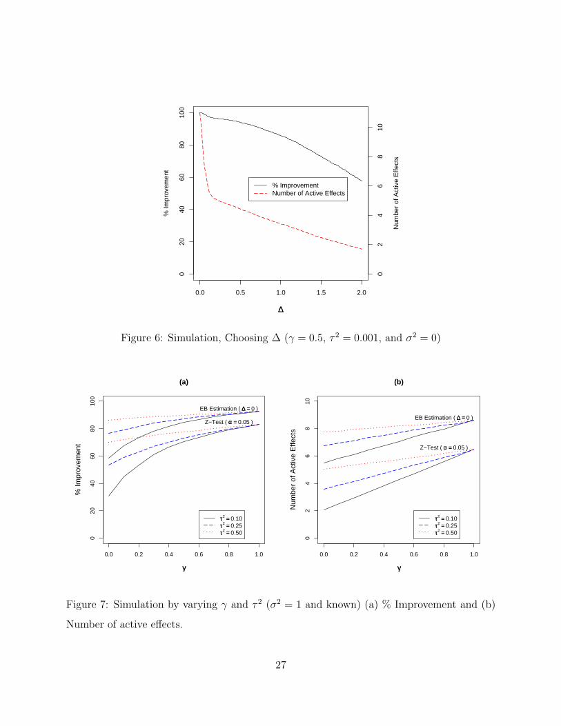
also reduced. Figure 6 shows the plot of these two metrics over ∆ when σ2 = 0. This figure

suggests that using a small value for ∆, a large reduction in the average Number of Active

Effects can be achieved while sacrificing only a small amount in % Improvement.

That the same patterns so far revealed in this section are reproducible for different

combinations of γ and τ 2 is illustrated in Figure 7. In this figure, the two metrics are

plotted as a function of γ. Each line represents a different value for τ 2, for either the usual

statistical test of significance procedure or EB estimation . In these plots, we fix σ2 = 1.

Also, the statistical significance level of α = .05 and practical significance level of ∆ = 0 are

used. Notice that for virtually any values of γ and τ 2, the % Improvement using the settings

suggested by EB estimation is superior to that when using the statistical z-test.

We also checked to see how the EB response estimates, after applying a practical sig-

nificance rule, compare with the least squares response estimates after applying statistical

testing. Table 4 provides mean squared error calculations from these simulations. We can

see that for these small values of ∆, the mean squared errors are generally much smaller

after using EB and these practical significance levels than with the models based on least

squares and statistical testing.

26

0.0 0.5 1.0 1.5 2.0

020

4060

8010

0

∆∆

% ImprovementNumber of Active Effects

02

46

810

% Im

prov

emen

t

Num

ber

of A

ctiv

e E

ffect

s

Figure 6: Simulation, Choosing ∆ (γ = 0.5, τ 2 = 0.001, and σ2 = 0)

0.0 0.2 0.4 0.6 0.8 1.0

020

4060

8010

0

(a)

γγ

% Im

prov

emen

t

EB Estimation ( ∆∆ == 0 )

Z−Test ( αα == 0.05 )

ττ2 == 0.10ττ2 == 0.25ττ2 == 0.50

0.0 0.2 0.4 0.6 0.8 1.0

02

46

810

(b)

γγ

Num

ber

of A

ctiv

e E

ffect

s

EB Estimation ( ∆∆ == 0 )

Z−Test ( αα == 0.05 )

ττ2 == 0.10ττ2 == 0.25ττ2 == 0.50

Figure 7: Simulation by varying γ and τ 2 (σ2 = 1 and known) (a) % Improvement and (b)

Number of active effects.

27

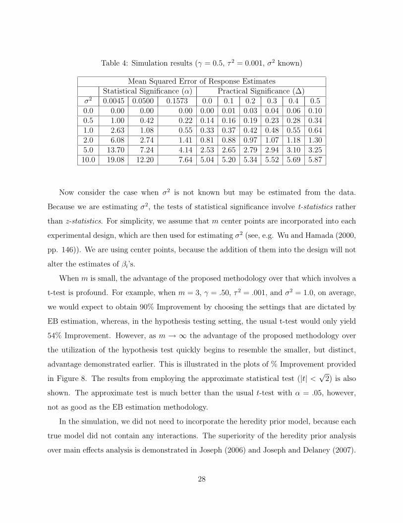
Table 4: Simulation results (γ = 0.5, τ 2 = 0.001, σ2 known)

Mean Squared Error of Response EstimatesStatistical Significance (α) Practical Significance (∆)

σ2 0.0045 0.0500 0.1573 0.0 0.1 0.2 0.3 0.4 0.50.0 0.00 0.00 0.00 0.00 0.01 0.03 0.04 0.06 0.100.5 1.00 0.42 0.22 0.14 0.16 0.19 0.23 0.28 0.341.0 2.63 1.08 0.55 0.33 0.37 0.42 0.48 0.55 0.642.0 6.08 2.74 1.41 0.81 0.88 0.97 1.07 1.18 1.305.0 13.70 7.24 4.14 2.53 2.65 2.79 2.94 3.10 3.2510.0 19.08 12.20 7.64 5.04 5.20 5.34 5.52 5.69 5.87

Now consider the case when σ2 is not known but may be estimated from the data.

Because we are estimating σ2, the tests of statistical significance involve t-statistics rather

than z-statistics. For simplicity, we assume that m center points are incorporated into each

experimental design, which are then used for estimating σ2 (see, e.g. Wu and Hamada (2000,

pp. 146)). We are using center points, because the addition of them into the design will not

alter the estimates of βi’s.

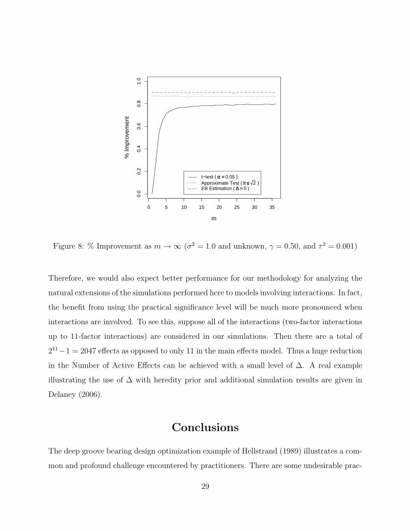
When m is small, the advantage of the proposed methodology over that which involves a

t-test is profound. For example, when m = 3, γ = .50, τ 2 = .001, and σ2 = 1.0, on average,

we would expect to obtain 90% Improvement by choosing the settings that are dictated by

EB estimation, whereas, in the hypothesis testing setting, the usual t-test would only yield

54% Improvement. However, as m → ∞ the advantage of the proposed methodology over

the utilization of the hypothesis test quickly begins to resemble the smaller, but distinct,

advantage demonstrated earlier. This is illustrated in the plots of % Improvement provided

in Figure 8. The results from employing the approximate statistical test (|t| <√

2) is also

shown. The approximate test is much better than the usual t-test with α = .05, however,

not as good as the EB estimation methodology.

In the simulation, we did not need to incorporate the heredity prior model, because each

true model did not contain any interactions. The superiority of the heredity prior analysis

over main effects analysis is demonstrated in Joseph (2006) and Joseph and Delaney (2007).

28

0 5 10 15 20 25 30 35

0.0

0.2

0.4

0.6

0.8

1.0

m

% Im

prov

emen

t

t−test ( αα == 0.05 )Approximate Test ( t ≤≤ 2 )EB Estimation ( ∆∆ == 0 )

Figure 8: % Improvement as m →∞ (σ2 = 1.0 and unknown, γ = 0.50, and τ 2 = 0.001)

Therefore, we would also expect better performance for our methodology for analyzing the

natural extensions of the simulations performed here to models involving interactions. In fact,

the benefit from using the practical significance level will be much more pronounced when

interactions are involved. To see this, suppose all of the interactions (two-factor interactions

up to 11-factor interactions) are considered in our simulations. Then there are a total of

211−1 = 2047 effects as opposed to only 11 in the main effects model. Thus a huge reduction

in the Number of Active Effects can be achieved with a small level of ∆. A real example

illustrating the use of ∆ with heredity prior and additional simulation results are given in

Delaney (2006).

Conclusions

The deep groove bearing design optimization example of Hellstrand (1989) illustrates a com-

mon and profound challenge encountered by practitioners. There are some undesirable prac-

29

tical consequences associated with the rigorous application of statistical hypothesis testing

procedures, in that it can prevent the gathering of sufficient guidance for the design process.

As is often the case, cost constraints keep the run size of an experiment quite small. In this

particular example, a small run size may be to blame for not being able to conclude from a

standard statistical test that two of the three factors are indeed significant. Unfortunately,

the usual recommendation to just “collect more data” is usually not a practical solution.

The engineer may have to make decisions with just the data that is presently available.

Another difficulty with statistical testing is the use of an α = .05 significance level, with-

out much reflection on what this actually means and whether it has any practical connection

with the problem at hand. In fact, if we are to rigorously adhere to the meaning of a test

of significance at the α = .05 level, then we would have to apply the correct simultaneous

testing procedure when we examine the size of multiple factorial effects; thereby magnifying

the probability we will be unable to identify any effects as significant.

In an optimization experiment, the sole objective is determining the particular factor

settings that will yield a desired response. In such a situation, we should be able to identify

an amount of improvement in the response that is not large enough to be of practical signifi-

cance. Thus, practical significance provides a much more meaningful criteria for determining

whether changing a factor’s setting is “worth it” than does a statistical significance level.

Further, when we focus on the objective of determining optimal factor settings, we might be

able to ignore other metrics for evaluating our estimation and model selection procedure.

The methodology we recommend for the analysis of optimization experiments centers

around an overall objective function which balances quality and cost. We suggest the EB

estimator presented in Joseph (2006) and Joseph and Delaney (2007) because of its many

desirable properties. It shrinks the coefficients and incorporates the effect hierarchy and

heredity principles. Based on these estimates, we may find the optimal settings for the

factors. Further, we may calculate the impact that a factor level change can have near this

optimal setting and determine whether this is large enough to be of practical interest.

We have demonstrated EB estimation using three different prior specifications. This

choice of prior has an effect on the final results. Our recommendation is to use the heredity

30

prior. However, the amount of computation involved in obtaining the estimates is much more

than for the other priors. When only a main effects model is considered, the use of either

the heredity or unequal variances prior leads to the same result. But when interaction and

polynomial terms are present in the model, the heredity prior should offer a more reasonable

and interpretable model. We have shown that when the unequal variances prior is used, the

EB estimator is the same as the beta coefficient method of Taguchi.

We found that statistical testing can be viewed as an approximation to the proposed

EB procedure. This is a very interesting and useful result because statistical testing in

general is much easier to implement than the EB procedure. We showed that using a z-

critical or t-critical value of√

2 in statistical testing approximates the EB procedure (with

the unequal variances prior). This leads to a statistical significance level that ranges from

15 to 40% depending on the error degrees of freedom. That this statistical significance

level is more liberal than the one that is universally used, and much more liberal than the

typical implementation for the simultaneous testing of multiple parameters, should come

as no surprise to practitioners experienced with analyzing engineering process optimization

experiments.

The simulation results provide support for the conclusion that the recommended method-

ology is superior to statistical hypothesis testing for identifying factor settings that, on av-

erage, yield response values closer to our objective without unduly increasing the cost. This

is the goal of optimization experiments.

Acknowledgments

The authors thank the Editor and a referee for their valuable comments and suggestions.

This research was supported by the U.S. National Science Foundation grant CMMI-0448774.

31

APPENDIX: Proof of Proposition 1

Proof: In order for the n × s matrix U to yield U ′U = nIs, it must be that s ≤ n.

When s < n, there exist orthogonal columns that can be appended to U , say V , such

that: W = [U , V ], where W is n × n and W ′W = nIn. Since we are not particularly

interested in the “effects” represented by the columns of V and as we demonstrate below,

the optimization problem is separable, we can extend the matrix Σ in an arbitrary way. Let

S = diag(τ 20 , . . . , τ 2

s−1, τ2s , . . . τ 2

n−1) represent the n × n prior covariance matrix for these n

orthogonal effects. In terms of these matrices, the marginal log-likelihood is

l = constant− 1

2log det

(WSW ′ + σ2In

)+ (y − µ01n)′(WSW ′ + σ2In)−1(y − µ01n).

Now, since W is orthogonal,

det(WSW ′ + σ2In

)=

n−1∏i=0

(nτ 2

i + σ2), (11)

and,

(WSW ′ + σ2In)−1 =1

n2WΛW ′,

where

Λ = diag

(n

nτ 20 + σ2

,n

nτ 21 + σ2

, . . . ,n

nτ 2n−1 + σ2

).

Let β = (W ′W )−1W ′y. So that,

(y − µ1n)′(WSW ′ + σ2In)−1(y − µ1n) =n−1∑i=0

n

nτ 2i + σ2

βi

2. (12)

Thus, from (11) and (12), we see that the finding of τ 2 that maximizes the integrated

likelihood is equivalent to solving the convenient separable optimization problem:

τ 2 = argminτ 2≥0

n−1∑i=0

[log(nτ 2

i + σ2) +n

nτ 2i + σ2

βi

2]

.

Differentiating with respect to τ 2i , we obtain the partial derivatives:

∂l

∂τ 2i

=n

nτ 2i + σ2

− n2

(nτ 2i + σ2)2

βi

2, for all i = 1, . . . , n− 1.

32

Setting the partial derivatives to zero and solving for τ 2i , yields n(nτ 2

i +σ2) = n2βi

2. So that

τ 2i =

(βi

2− σ2

n

)+

is feasible.

Plugging in the EB estimators τ 2i , for all i = 0, . . . n− 1, into (3) yields:

β = SW ′(WSW ′ + σ2In

)−1

(y − µ01n)

= diag

(nτ 2

0

nτ 20 + σ2

,nτ 2

1

nτ 21 + σ2

, . . . ,nτ 2

n−1

nτ 2n−1 + σ2

)β.

Note that when nβi

2> σ2, we have nτ 2

i /(nτ 2i + σ2) = 1 − 1/z2

i , and when nβi

2< σ2, we

have nτ 2i /(nτ 2

i + σ2) = 0. Therefore,

βi = (1− 1

z2i

)+βi for all i = 0, . . . , n− 1.

And if the effects βs, . . . , βn−1 are not of interest, then they can simply be ignored. ♦

References

Berger, J. O. (1985). Statistical Decision Theory and Bayesian Analysis. Springer, New

York, NY.

Box, G. E. P.; Hunter, J. S.; and Hunter, W. G. (2005). Statistics for Experimenters.

Wiley, New York, NY, 2nd edition.

Box, G. E. P. and Meyer, R. D. (1993). “Finding the Active Factors in Fractionated

Screening Experiments”. Journal of Quality Technology, 25, pp. 94–105.

Breiman, L. (1995). “Better Subset Regression Using the Nonnegative Garrote”. Techno-

metrics, 37, pp. 373–384.

Carlin, B. P. and Louis, T. A. (2000). Bayes and Empirical Bayes Methods for Data

Analysis. Chapman and Hall/CRC, Boca Raton, FL.

Chipman, H.; Hamada, M.; and Wu, C. F. J. (1997). “A Bayesian Variable-Selection

Approach for Analyzing Designed Experiments With Complex Aliasing”. Technometrics,

39, pp. 372–381.

33

Daniel, C. (1959). “Use of Half-Normal Plots in Interpreting Factorial Two-Level Experi-

ments”. Technometrics, 1, pp. 311–341.

Delaney, J. D. (2006). Contributions to the Analysis of Experiments Using Empirical

Bayes Techniques. PhD thesis, Georgia Institute of Technology, Atlanta, GA.

Efron, B.; Johnstone, I.; Hastie, T.; and Tibshirani, R. (2004). “Least Angle

Regression”. Annals of Statistics, 32, pp. 407–499.

Gruber, M. (1998). Improving Efficiency By Shrinkage. Marcel Dekker, New York, NY.

Hamada, M. and Balakrishnan, N. (1998). “Analyzing Unreplicated Factorial Exper-

iments: A Review With Some New Proposals”. Statistica Sinica, 8(11), pp. 1–41.

Hamada, M. and Wu, C. F. J. (1992). “Analysis of Designed Experiments With Complex

Aliasing”. Journal of Quality Technology, 24, pp. 130–137.

Hellstrand, C. (1989). “The Necessity of Modern Quality Improvement and Some Expe-

rience With its Implementation in the Manufacture of Rolling Bearings [and Discussion]”.

Philosophical Transactions of the Royal Society of London, Series A, Mathematical and

Physical Sciences, 327(1596), pp. 529–537.

Joseph, V. R. (2004). “Quality Loss Functions for Nonnegative Variables and Their Ap-

plications”. Journal of Quality Technology, 32, pp. 129–138.

Joseph, V. R. (2006). “A Bayesian Approach to the Design and Analysis of Fractionated

Experiments”. Technometrics, 48, pp. 219–229.

Joseph, V. R. and Delaney, J. D. (2007). “Functionally Induced Priors for the Analysis

of Experiments”. Technometrics, 49, pp. 1–11.

Kennedy, W. J. and Bancroft, T. A. (1971). “Model Building For Prediction in

Regression Based Upon Repeated Significance Tests”. Annals of Mathematical Statistics,

42, pp. 1273–1284.

34

Lehmann, E. and Casella, G. (1998). Theory of Point Estimation. Springer, New York,

NY, 2nd edition.

Lenth, R. V. (1989). “Quick and Easy Analysis of Unreplicated Factorials”. Technometrics,

31, pp. 469–473.

Meyer, R. D.; Steinberg, D. M.; and Box, G. (1996). “Follow-up Designs to Resolve

Confounding in Multifactor Experiments, (with discussion)”. Technometrics, 38, pp. 303–

332.

Miro-Quesada, G.; Del Castillo, E.; and Peterson, J. J. (2004). “A Bayesian

Approach for Multiple Response Surface Optimization in the Presence of Noise Variables”.

Journal of Applied Statistics, 31(3), pp. 251–270.

Montgomery, D. C. (2004). Design and Analysis of Experiments. Wiley, New York, NY.

Myers, R. H. and Montgomery, D. C. (2002). Response Surface Methodology. New

York: Wiley, 2nd edition.

Peterson, J. J. (2004). “A Posterior Predictive Approach to Multiple Response Surface

Optimization”. Journal of Quality Technology, 36(2), pp. 139–153.

Rajagopal, R. and Del Castillo, E. (2005). “Model-Robust Process Optimization

Using Bayesian Model Averaging”. Technometrics, 47, pp. 152–163.

Taguchi, G. (1987). System of Experimental Design, Vol. 1 & Vol. 2. Unipub/Kraus

International, White Plains, NY.

Tibshirani, R. (1996). “Regression Shrinkage and Selection via the LASSO”. Journal of

the Royal Statistical Society, Sec. B, 58, pp. 267–288.

Wu, C. F. J. and Hamada, M. (2000). Experiments: Planning, Analysis, and Parameter

Design Optimization. Wiley, New York, NY.

35