Analysis of Record and Playback Errors of GPS Signals Caused by the USRP

by

Andrew Hennigar

A thesis submitted to the Graduate Faculty ofAuburn University

in partial ful�llment of therequirements for the Degree of

Master of Science

Auburn, AlabamaDecember 13 ,2014

Keywords: USRP Error, Clock Synchronization, Software Receiver, IF

Copyright 2014 by Andrew Hennigar

Approved by:

David M. Bevly, Chair, Professor of Mechanical EngineeringLloyd Riggs, Professor of Electrical and Computer EngineeringShiwen Mao, Professor of Electrical and Computer Engineering

Abstract

In this thesis, the errors created by the USRP (Universal Software Receiver Platform)

during record and playback are analyzed. The USRP is used for jamming, spoo�ng, and

GPS processing, and has recently become widely used for capturing GPS signals for record

and playback. However, there has been little research into how the USRP e�ects signal

quality during record and playback.

This thesis is based on the live capture of L1 GPS signals. Data is captured for multiple

scenarios in both static and dynamic situations. The signal is split and sent to multiple

receivers and the USRP. The data is gathered, parsed, and quanti�ed using statistical analysis

for comparison over a broad range of tests.

From the captured signals, statistical analysis is used for a more comprehensive overview

of the USRP. Results show that statistical data from playback of GPS signals is reliable in

multiple scenarios, thus validation the USRP as an accurate means by which data can be

recorded and played back.

ii

Acknowledgments

I want to start of by giving God all the glory for this paper. Every opportunity given

to me was through Him and I am so thankful. I want to thank my wife for love support and

understanding. Without the support of my better half I would not have completed this in

a timely fashion. I want to thank Dr. Bevly for his support, always willing to allow me to

bounce ideas o� of him and for the opportunities he has given to me. I also want to give a

shout out to Scott, Jordan, and the rest of the lab for helping me over the mental blocks I

have had along the way.

iii

Contents

Abstract . . . . . . . . . . . . . . . . . . . . . . . . . . . . . . . . . . . . . . . . . . . ii

Acknowledgments . . . . . . . . . . . . . . . . . . . . . . . . . . . . . . . . . . . . . . iii

List of Figures . . . . . . . . . . . . . . . . . . . . . . . . . . . . . . . . . . . . . . . vii

List of Tables . . . . . . . . . . . . . . . . . . . . . . . . . . . . . . . . . . . . . . . . x

1 Introduction/Terms . . . . . . . . . . . . . . . . . . . . . . . . . . . . . . . . . . 1

1.1 Motivation . . . . . . . . . . . . . . . . . . . . . . . . . . . . . . . . . . . . . 1

1.2 Key Terms . . . . . . . . . . . . . . . . . . . . . . . . . . . . . . . . . . . . . 1

1.3 Previous Work . . . . . . . . . . . . . . . . . . . . . . . . . . . . . . . . . . 4

1.4 GPS Background Information . . . . . . . . . . . . . . . . . . . . . . . . . . 8

1.4.1 GPS Position Calculation . . . . . . . . . . . . . . . . . . . . . . . . 9

1.4.2 GPS Signal Structure . . . . . . . . . . . . . . . . . . . . . . . . . . . 11

1.5 Contributions . . . . . . . . . . . . . . . . . . . . . . . . . . . . . . . . . . . 13

1.6 Thesis Outline . . . . . . . . . . . . . . . . . . . . . . . . . . . . . . . . . . 13

2 USRP Background . . . . . . . . . . . . . . . . . . . . . . . . . . . . . . . . . . 14

2.1 USRP Hardware . . . . . . . . . . . . . . . . . . . . . . . . . . . . . . . . . 14

2.2 USRP Software Interface . . . . . . . . . . . . . . . . . . . . . . . . . . . . . 16

2.3 External Hardware/Software . . . . . . . . . . . . . . . . . . . . . . . . . . . 18

3 USRP and GPS Receiver Static Data Research . . . . . . . . . . . . . . . . . . 20

3.1 Static Testing Comparison Between GPSDO and Internal USRP Clock . . . 20

3.1.1 Static Setup . . . . . . . . . . . . . . . . . . . . . . . . . . . . . . . . 20

3.1.2 Static Results without GPSDO . . . . . . . . . . . . . . . . . . . . . 22

3.1.3 Static Results with GPSDO . . . . . . . . . . . . . . . . . . . . . . . 26

3.1.4 Statistics with GPSDO . . . . . . . . . . . . . . . . . . . . . . . . . . 29

iv

3.1.5 Static Conclusions with and without GPSDO . . . . . . . . . . . . . 30

3.2 CSAC Timing . . . . . . . . . . . . . . . . . . . . . . . . . . . . . . . . . . . 31

3.2.1 Background . . . . . . . . . . . . . . . . . . . . . . . . . . . . . . . . 31

3.2.2 Hardware Setup . . . . . . . . . . . . . . . . . . . . . . . . . . . . . . 31

3.2.3 Results . . . . . . . . . . . . . . . . . . . . . . . . . . . . . . . . . . . 32

3.2.4 Statistics . . . . . . . . . . . . . . . . . . . . . . . . . . . . . . . . . . 35

3.2.5 Conclusions . . . . . . . . . . . . . . . . . . . . . . . . . . . . . . . . 35

3.3 Repeatability of Record and Playback with the USRP N210 . . . . . . . . . 36

3.3.1 GPSDO GPS vs Non-GPS . . . . . . . . . . . . . . . . . . . . . . . . 36

3.3.2 Repeatability Di�erences . . . . . . . . . . . . . . . . . . . . . . . . . 37

3.3.3 Statistics . . . . . . . . . . . . . . . . . . . . . . . . . . . . . . . . . . 38

3.3.4 Repeatability Between Receivers . . . . . . . . . . . . . . . . . . . . . 39

3.3.4.1 Results . . . . . . . . . . . . . . . . . . . . . . . . . . . . . 39

3.3.5 Conclusions . . . . . . . . . . . . . . . . . . . . . . . . . . . . . . . . 40

3.4 Pseudorange and Lower Level Measurements . . . . . . . . . . . . . . . . . . 40

3.4.1 Background Work . . . . . . . . . . . . . . . . . . . . . . . . . . . . . 41

3.4.2 Results . . . . . . . . . . . . . . . . . . . . . . . . . . . . . . . . . . . 41

3.4.3 Statistics . . . . . . . . . . . . . . . . . . . . . . . . . . . . . . . . . . 47

3.4.4 Conclusions . . . . . . . . . . . . . . . . . . . . . . . . . . . . . . . . 47

4 Dynamic Testing . . . . . . . . . . . . . . . . . . . . . . . . . . . . . . . . . . . 48

4.1 Data gathered . . . . . . . . . . . . . . . . . . . . . . . . . . . . . . . . . . . 48

4.1.1 Dynamic Data Analysis Using internal USRP clock . . . . . . . . . . 50

4.1.2 Dynamic Data Analysis Using GPSDO . . . . . . . . . . . . . . . . . 53

4.1.2.1 High Dynamic Testing . . . . . . . . . . . . . . . . . . . . . 56

4.1.3 Statistics . . . . . . . . . . . . . . . . . . . . . . . . . . . . . . . . . . 59

4.2 Dynamic Conclusions . . . . . . . . . . . . . . . . . . . . . . . . . . . . . . . 60

5 Analysis of USRP Record and Playback Using a Software Receiver . . . . . . . 62

v

5.1 GPS Software Receiver Background . . . . . . . . . . . . . . . . . . . . . . . 62

5.1.1 How receivers work in general . . . . . . . . . . . . . . . . . . . . . . 62

5.2 Software Receiver Selection . . . . . . . . . . . . . . . . . . . . . . . . . . . 65

5.3 Drawbacks . . . . . . . . . . . . . . . . . . . . . . . . . . . . . . . . . . . . . 66

5.4 Software Receiver Uses . . . . . . . . . . . . . . . . . . . . . . . . . . . . . . 67

5.5 Results From the Software Receivers . . . . . . . . . . . . . . . . . . . . . . 67

5.6 Conclusions . . . . . . . . . . . . . . . . . . . . . . . . . . . . . . . . . . . . 69

6 Conclusions and Future Work . . . . . . . . . . . . . . . . . . . . . . . . . . . . 70

6.1 Observations and Conclusions . . . . . . . . . . . . . . . . . . . . . . . . . . 70

6.1.1 Limitations of USRP Evaluation . . . . . . . . . . . . . . . . . . . . . 70

6.1.2 Conclusions . . . . . . . . . . . . . . . . . . . . . . . . . . . . . . . . 71

6.2 Future Work . . . . . . . . . . . . . . . . . . . . . . . . . . . . . . . . . . . . 73

6.2.1 Measuring Di�erence Between Clocks . . . . . . . . . . . . . . . . . . 73

6.2.2 From IF to Pseudorange . . . . . . . . . . . . . . . . . . . . . . . . . 73

6.2.3 GPS Simulator . . . . . . . . . . . . . . . . . . . . . . . . . . . . . . 73

6.2.4 Mitigating Error . . . . . . . . . . . . . . . . . . . . . . . . . . . . . 73

Bibliography . . . . . . . . . . . . . . . . . . . . . . . . . . . . . . . . . . . . . . . . 74

Bibliography . . . . . . . . . . . . . . . . . . . . . . . . . . . . . . . . . . . . . . . . 75

vi

List of Figures

1.1 Graphical Example of the Three GPS Signals . . . . . . . . . . . . . . . . . 11

2.1 USRP Circuit Diagram . . . . . . . . . . . . . . . . . . . . . . . . . . . . . . 15

2.2 GNU Radio Companion . . . . . . . . . . . . . . . . . . . . . . . . . . . . . 17

3.1 Static GPS Hardware Setup . . . . . . . . . . . . . . . . . . . . . . . . . . . 21

3.2 Data Collection Point for Static Position Analysis . . . . . . . . . . . . . . . 22

3.3 Position Di�erenced From Actual Position With Internal USRP Clock . . . . 24

3.4 Di�erence Between Live and Playback Position With Internal USRP Clock . 25

3.5 Static Test With GPSDO . . . . . . . . . . . . . . . . . . . . . . . . . . . . 26

3.6 Position Di�erenced From Actual Position With GPSDO . . . . . . . . . . . 27

3.7 Di�erence Between Live and Playback Position With GPSDO . . . . . . . . 28

3.8 Static Live vs Playback PSD of Position . . . . . . . . . . . . . . . . . . . . 28

3.9 Comparison of C/No with GPSDO with GPS . . . . . . . . . . . . . . . . . 29

3.10 Di�erenced of C/No with GPSDO with GPS . . . . . . . . . . . . . . . . . . 29

3.11 Static Hardware Setup with CSAC . . . . . . . . . . . . . . . . . . . . . . . 32

3.12 North and East Position with CSAC . . . . . . . . . . . . . . . . . . . . . . 32

3.13 First 500 Seconds of Playback with CSAC . . . . . . . . . . . . . . . . . . . 33

3.14 After First 500 Seconds of Playback with CSAC . . . . . . . . . . . . . . . . 34

3.15 Live and Playback Di�erenced with CSAC . . . . . . . . . . . . . . . . . . . 34

3.16 Live vs Playback PSD of Position with CSAC . . . . . . . . . . . . . . . . . 35

3.17 Repeatability Test With and Without GPS Aided GPSDO Timing . . . . . . 37

vii

3.18 Repeatability Test Di�erenced . . . . . . . . . . . . . . . . . . . . . . . . . . 38

3.19 Repeatability Test Di�erenced . . . . . . . . . . . . . . . . . . . . . . . . . . 39

3.20 Pseudorange Measurements Live and Playback . . . . . . . . . . . . . . . . . 42

3.21 All Pseudoranges Di�erenced 13SVs . . . . . . . . . . . . . . . . . . . . . . . 43

3.22 Enhanced Di�erence Between Pseudorange Measurements 13SVs . . . . . . . 43

3.23 Pseudorange to Live Vs Playback . . . . . . . . . . . . . . . . . . . . . . . . 44

3.24 Raw Doppler Measurements . . . . . . . . . . . . . . . . . . . . . . . . . . . 44

3.25 All Di�erenced Doppler Measurements . . . . . . . . . . . . . . . . . . . . . 45

3.26 Clock Drift Observed from Di�erencing . . . . . . . . . . . . . . . . . . . . . 46

3.27 Carrier to Noise Doppler Measurements . . . . . . . . . . . . . . . . . . . . . 46

4.1 Dynamic Path . . . . . . . . . . . . . . . . . . . . . . . . . . . . . . . . . . . 49

4.2 Vehicle Used for Dynamic Test Data collection . . . . . . . . . . . . . . . . . 50

4.3 Dynamic Position Di�erenced From Actual Position With Internal USRP Clock 51

4.4 Dynamic Di�erence Between Live and Playback Position With Internal USRPClock . . . . . . . . . . . . . . . . . . . . . . . . . . . . . . . . . . . . . . . . 52

4.5 Dynamic Comparison of C/No without GPSDO . . . . . . . . . . . . . . . . 53

4.6 Dynamic Di�erenced of C/No without GPSDO . . . . . . . . . . . . . . . . 53

4.7 Dynamic Test With GPSDO . . . . . . . . . . . . . . . . . . . . . . . . . . . 54

4.8 Dynamic Position Di�erenced From Actual Position With GPSDO . . . . . . 54

4.9 Dynamic Di�erence Between Live and Playback Position With GPSDO . . . 55

4.10 Dynamic Live vs Playback PSD of Position . . . . . . . . . . . . . . . . . . . 55

4.11 Dynamic Comparison of C/No with GPSDO . . . . . . . . . . . . . . . . . . 56

4.12 Dynamic Di�erenced of C/No with GPSDO . . . . . . . . . . . . . . . . . . 56

4.13 High Dynamic Path . . . . . . . . . . . . . . . . . . . . . . . . . . . . . . . . 57

4.14 High Dynamic 2D Position with All 3 . . . . . . . . . . . . . . . . . . . . . . 58

viii

4.15 High Dynamic Ublox Live vs Ublox Playback . . . . . . . . . . . . . . . . . 59

5.1 Series Acquisition . . . . . . . . . . . . . . . . . . . . . . . . . . . . . . . . . 63

5.2 Series Acquisition 10Ms . . . . . . . . . . . . . . . . . . . . . . . . . . . . . 63

5.3 Sub Frames of GPS Ephemeris Message[2] . . . . . . . . . . . . . . . . . . . 65

5.4 Live Software Receiver Data with and Without ampli�er . . . . . . . . . . . 67

5.5 Live Software Receiver Data Without ampli�er . . . . . . . . . . . . . . . . . 68

ix

List of Tables

1.1 Error Model Statistics for Paper Markov Processes . . . . . . . . . . . . . . 5

1.2 Averaged Frequency O�set and Drift Rate . . . . . . . . . . . . . . . . . . . 7

3.1 2D GPS Statistics for Static Data With Internal USRP Clock . . . . . . . . 25

3.2 Latitude and Longitude GPS Statistics for Static Data with GPSDO . . . . 30

3.3 2D GPS Statistics for Static Data with GPSDO . . . . . . . . . . . . . . . . 30

3.4 CSAC Record and Playback Data . . . . . . . . . . . . . . . . . . . . . . . . 35

3.5 CSAC Compared to Static with GPSDO . . . . . . . . . . . . . . . . . . . . 36

3.6 Error Statistics for Repeatability . . . . . . . . . . . . . . . . . . . . . . . . 38

3.7 2D GPS Statistics for Static Data with GPSDO . . . . . . . . . . . . . . . . 40

3.8 Pseudorange Statistics . . . . . . . . . . . . . . . . . . . . . . . . . . . . . . 47

3.9 Doppler Di�erence Statistics . . . . . . . . . . . . . . . . . . . . . . . . . . . 47

4.1 2D GPS Statistics for Data with no GPSDO . . . . . . . . . . . . . . . . . . 52

4.2 Maximum Error Spikes Caused by USRP without GPSDO . . . . . . . . . . 52

4.3 Latitude and Longitude GPS Statistics for Dynamic Data with GPSDO . . . 59

4.4 2D GPS Statistics for Dynamic Data with GPSDO . . . . . . . . . . . . . . 60

4.5 High Dynamic Statistics . . . . . . . . . . . . . . . . . . . . . . . . . . . . . 60

5.1 Software Receiver vs. Static Data . . . . . . . . . . . . . . . . . . . . . . . . 69

x

Chapter 1

Introduction/Terms

This thesis will begin by explaining the USRP (Universal Software Radio Peripheral)

in depth. Previous research that has in�uenced this work and vital terms will be de�ned.

This section is concluded with a discussion about the hardware and software to give a better

understanding of the equipment used for data collection.

1.1 Motivation

The USRP is used for record and playback of signals in many projects. It is very useful

when working with unique signals. Though some noise statistics are known about the USRP,

no study has been done on the repercussions of recording and playing back GPS signals. This

thesis focuses on live IF (Intermediate Frequency) data and the error or changes the USRP

makes to this data during record and playback. The validity of recording and playing back

data is veri�ed with this real data.

Because of the many applications in which the USRP is used, there is also a need for an

understanding of how di�erent scenarios change the results from the USRP di�erently. The

multiple scenarios used in this thesis represent a subset of data that can be collected by the

USRP. Most of these scenarios are changes in hardware during record and playback. In an

attempt to keep the experimentation to a level used by most people, this thesis will focus

on L1 GPS signals for record and playback.

1.2 Key Terms

In this section important terms used in this thesis are de�ned and their uses are dis-

cussed. There are many components to the USRP that need to be known before using the

1

equipment; this section will break down and de�ne the components of the USRP and their

purposes.

The USRP is a widely known, highly used �software radio�, meaning it is software

programmable. The USRP has a motherboard with an FPGA (Field Program Gate Array)

which can be reprogrammed and has fast computation capabilities. The USRP also requires

a daughterboard, which is the customizable front end for this receiver. The motherboard and

daughterboard are combined as a completed USRP, which is then connected to a computer in

order to record data at high speed via a gigabit ethernet cable. The recording can be sent to

the onboard hard drive or external drive via USB 3.0 to be used at a later date. The WBX

daughterboard is a broadband front end that can accept frequencies between 50Mhz and

2.2Ghz. It can receive and transmit from the same board and has a bandwidth of 40Mhz.

This makes it ideal for GPS because it can cover all GPS frequencies and bandwidths. With

multiple USRPs, all GPS frequencies can be captured and played back to create a live sky

scenario. This has to be done with multiple USRP's because the bandwidth does not allow

for L1, L2 and L5 to be received simultaneously on one daughterboard.

The FPGA on the motherboard is one of the most important components of the USRP.

The FPGA is a reprogrammable hardware chip which can be used many times and in multiple

ways. It is a series of silicon gates that can be either opened or closed depending on what is

needed. The FPGA is a vital for capturing data at the high sample rate required for GPS.

The clock on the motherboard is used to sample data. The standard USRP clock is a

100 Hz TCXO (Temperature Controlled Crystal Oscillator), and the TCXO measures the

oscillation of an open crystal that changes with temperature. The TCXO is one of the least

accurate clocks available, and when working with GPS another clock may be needed. The

frequency accuracy of the TCXO on the USRP is 2.5 ppm (Parts Per Million) ,which is a

measurement of the variation in the clock over time.

The GPSDO is an option that can be added to the USRP. The GPSDO (GPS Disciplined

Oscillator) is an OCXO (Oven Controlled Crystal Oscillator) with a GPS receiver to give

2

GPS time corrections. The OCXO is 100 times more accurate than the TCXO at about

.025 ppm for the OCXO by itself. The OCXO outputs a 10 MHz signal which will discipline

the TCXO on the motherboard. The GPSDO has a Ublox receiver onboard that GPS time

updates; these time updates are used to discipline the onboard OCXO, making it accurate

to .01 ppm. The GPSDO is used in experiments for this thesis, and shows a great deal more

accuracy for position measurements.

A completely external clock called the CSAC (Chip Scaled Atomic Clock) is also inves-

tigated. The CSAC is much more accurate than the OCXO. This clock uses cesium atoms

to keep time instead of an oscillating crystal. This clock, though much more accurate than

the GPSDO, may not change the position accuracy from the USRP. This clock will also be

tested and compared to the TCXO and GPSDO.

There are many designations of time when working with GPS. The two used in this

work are GPS time and UTC time. The GPS time is of the format week number and week

seconds. This gives the number of weeks since the beginning of GPS time and the number of

seconds from midnight Sunday of a new week. UTC (Coordinated Universal Time) or GMT

(Greenwich Mean Time) is the worldwide standard time. This time is based on a 24 hour

clock and is much easier to keep track of than GPS time. Both types of time are important

in this project to keep track of the data being captured to make sure everything is taken at

the same time.

When calculating GPS positions multiple lower level measurements are used. In this

thesis, some of these measurements are explored to get a more comprehensive overview of

the error created by the USRP. The �rst measurements discussed are pseudoranges. The

pseudoranges are used to calculate the position of the GPS receiver. The pseudorange is

a range between the satellite and receiver plus errors that will be discussed in Section 1.4.

These measurements are used in most receivers, but the Ublox does not automatically output

these measurements. To record the pseudoranges a software package called Go-GPS is used

in congruence with Matlab.

3

Another measurement used in this thesis is the doppler measurement. The doppler

measurement is the quanti�cation of doppler shift from the motion of the satellites. The

doppler measurements are explored in this thesis because they are much noisier than the

pseudorange measurements. The doppler measurements are measurements used to calculate

the velocity of the receiver. The �nal measurement used is the carrier to noise measurement.

This is the ratio of the signal power to the noise power. This measurement can show a broad

spectrum of the noise and how the USRP increases the noise during record and playback.

1.3 Previous Work

The USRP is a simplistic piece of hardware that is inexpensive to purchase. Because of

this, it has been used by many people for many di�erent applications. The papers discussed

in this section provide concepts for testing and for future work.

As is well known, GPS signals have error associated with them. Many of the errors are

modeled while others are incapable of being modeled. To understand the errors created by

the USRP it is �rst imperative to get a basic understanding of the errors on the GPS signals.

One paper that discusses this is [16], which goes into details about the error statistics and

types on the pseudoranges and how the error changes with di�erent types of receivers. The

paper also gives statistics of the Markov processes they use to model the error. The errors

have been tabulated in Table 1.1 from [16]. Each statistic shown in Table 1.1 corresponds

to error in the pseudoranges caused by the individual sources mentioned. Looking at the

pseudoranges can show other sources of error when the known errors can be accounted for.

4

Table 1.1: Error Model Statistics for Paper Markov ProcessesError Parameter Std. Dev. (meters) Time(s)

Ephemeris 3.0 1800Ionosphere 5.0 1800Troposphere 2.0 3600

Multipath, C/A Standard 5.0 600Multipath, C/A Narrow 0.25 600

Multipath, P 1.0 600Multipath, L1 carrier 0.048 600Selective Availability 30.0 180

To start the work with the USRP, a proper setup was required. Because the USRP

is inexpensive and not explicitly designed to record GPS, some modi�cations were required

to the USRP. First, a daughterboard was chosen based on bandwidth and record and play-

back capability. The WBX daughterboard was chosen and validated in [6],which also shows

Matlab as a usable software package and useful when trying to simulate GPS signals in the

future.

In the past, before the availability of the USRP N210, the standard USRP was used. To

get a signal that is viable the author in [19] required the use of an external down converter

for the signal. The work converted the signal from the 1.5 GHz to the IF frequency 915

MHz. Their daughterboard takes in a frequency ranged of 750-1050 MHz and mixes it

down to baseband. They up convert the base band data in Matlab to an IF of 1 MHz as

shown in Equation (1.1) where fm = 1MHz and fs = 4MHz the up conversion allows the

multiplication coe�cients to be zeroes and ±1.

y = Icos(2πnfmfs

)−Qsin(2πnfmfs

) (1.1)

As noted, the USRP signal needs to be slightly modi�ed for it to be useful when recorded.

Many di�erent methods are used, most of which involve ampli�cation and �ltering as noted

in [11]. A method similar to [11] with a 30dB low noise ampli�er and a band pass �lter

5

was initially used. Through experimental means an alternative method used with one active

antenna was devised.

Some of the error created by the USRP is created in the following ways: the sampling

procedure, the process noise in the USRP, and the clock noise of the USRP. When looking

into these various errors, research was initially conducted on the e�ect of clock noise; this

was chosen as the �rst study for noise because of its signi�cance in GPS solutions. Many

papers discuss the error created by the USRP clock during sampling. One such paper, [18],

discusses a study done on L1 and L2 from one satellite that compares measurements capture

from the TCXO and OCXO. Building on this with this in [10] discusses a software receiver

and the di�erences between external clock options. The frequency instability of an oscillator

in terms of instantaneous, normalized frequency deviation y(t) is in Equation 1.2, where f(t)

is the instantaneous frequency and f0 is the nominal frequency. In [10] they discuss where

errors occur in a software receiver.

y(t) =f(t)− f0

f0, (1.2)

∆fIF = fIF − ˆfIF = r∆fS + δ (1.3)

In Equation 1.3 the δ is error due to imperfection of the frequency synthesizer, which is

basically error caused by the clock. The research in [10] uses a simulator, so any error in the

wave is synthesized and can be set to zero. Therefore the main error is the clock error from

the simulator and receiver. The clock error can be modeled in discrete time using the �rst

order Taylor series (Equation 1.4 ) where y0 is the initial fractional frequency error, z0 is the

initial linear frequency drift rate, τ is the time interval of the frequency error measurements,

wn is the frequency process noise. the fractional frequency deviation measurement sn is the

sum of yn the frequency deviation and the zero mean measurement noise vn.

yn = y0 + z0τn+ wn (1.4)

6

yn =N−1∑i=0

h1isn−i (1.5)

From this the clock mode estimation (Equation 1.5) is derived, and from the tests run, the

statistics for all three types of clocks used is shown in Table 1.2.

Table 1.2: Averaged Frequency O�set and Drift RateOscillator Rb OCXO TCXO

Mean (yn) -4.08e-10 -4.48e-8 6.63e-7Mean (zn) 1.0363e-15 -2.6299e-14 6.9867e-13

This table shows the average error from the clock. As can be seen, the TCXO is about

10 times worse than the OCXO. This will translate to error in position calculations because

of the need for accurate timing when doing GPS calculations.

Although in [10] the writers discussed a rubidium oscillator as the atomic clock, this

thesis uses a CSAC (Chip Scale Atomic Clock). For the statistics and background on the

CSAC, the Symmetricon paper [12] was studied. The idea behind the CSAC clock was to get

a small very accurate clock that does not use a signi�cant amount of power. The CSAC has

a low power TCXO that outputs a signal to the microwave synthesizer that keeps the time

with cesium atoms. For a short time span the CSAC has an Alan variance with distribution

medians for a time constant of 10 seconds of 2.4X10−11. This is comparable to the required

timing accuracy of GPS of nanosecond level.

There is always a need for low cost GPS simulators. Because this thesis focuses on

the noise created by the USRP, one of the goal uses for this thesis will be with a GPS

simulator using the USRP. Navsys has software and hardware packages that can be used

for recording, playing back, jamming, spoo�ng and simulating GPS with the USRP. The

paper focuses on the uses of Matlab in [7], [5], and [4]. Each paper discussed advancements

in the area of simulation and recording. In [5] the paper focuses on the simulation of more

complicated signals including scintillation, but the drawback is the information has to be

dealt with digitally. This hardware package cannot playback, on the other hand in [4] a

hybrid simulator/receiver is discussed which can playback recorded data but not simulated

7

data. From these papers a need for simplistic simulators that can playback data to a hardware

receiver is discovered.

Other papers focus on methods to interfere with the GPS signal. There is always needs

for a low cost, portable, and �exible GNSS signal and interference signal generator. The

main receiver used to verify the ability of the interference signal generator is a Novatel. In

the paper [8] many signals were simulated to show that there are a number of possibilities

for simulations.

Jamming is not only an issue with GPS, it also is an issue in standard radio. The

methods in [15] use a spread spectrum technique to make the signal more robust. The

USRP is used to place the code on the broadband signal because of its ability to process

data at such a fast pace. This paper concluded that the USRP is a good multiuse platform.

The USRP is also being used for mitigating RF interferences. In the system presented

in [13] a USRP1 with a WBX daughterboard is used to identify the interference signals and

remove it. These experiments were done on the GPS frequency but at a much higher power

than GPS. A BPSK (Binary Phase Shift Keying) signal is created and transmitted with a

second signal attempting to corrupt it. The algorithm used has a reference signal vector,

which the cost function is based o� of. The main disadvantage of this is that the pro�le

required for the USRP to recognize the proper signal will knock out more powerful signals.

All GPS signals are encoded with Pseudorandom noise, in the paper [14] they discuss

the errors caused by I/Q imbalances created by the USRP. In this paper the errors discussed

are caused by encoded messages over multiple frequencies. This is important when dealing

with Dual Frequency (L1/L2) messages and shows another method of USRP error creation.

1.4 GPS Background Information

As mentioned earlier this thesis details how the USRP works with GPS record and

playback. To understand how this works, some basic GPS needs to be discussed.

8

1.4.1 GPS Position Calculation

To get a GPS position solution, a method called trilateralization is used. For a position

solution from the signals, four GPS satellites are required. These satellite positions are

calculated from the ephemeris that they transmit. Knowing the position of the satellites,

clock bias of the satellites, and the pseudoranges between each satellite and receiver, a

position solution can be calculated. The general way to solve for the position solutions is

shown in formula in Equations (1.6 - 1.13). The actual range between the receiver and the

satellite positions is seen in (1.6). This range is calculated from the satellite positions and

an estimate of the receiver position.

range =√

(x− satpositionx)2 + (y − satpositiony)2 + (z − satpositionz)2 (1.6)

From this range calculated in (1.6) and the positions of the satellites and receiver the

unit vectors to each satellite are calculated. The unit vectors seen in (1.7) are used in the

least squares calculations to estimate the receiver positions.

ux

uy

uz

=

(x− satpositionx)/range

(y − satpositiony)/range

(z − satpositionz)/range

(1.7)

The H matrix (1.8) is a matrix of the unit vectors to each satellite and a row of ones

for estimation of the clock bias.

H =

ux1 uy1 uz1 1

......

......

uxn uyn uzn 1

(1.8)

9

The position vector in Equation (1.9) plus the clock term is estimated each iteration.

With the least squares method the position solution is generally acceptable within �ve iter-

ation.

ˆpos =

x

y

z

cdt

(1.9)

The estimated pseudoranges are calculated in Equation (1.10) where the cdt is the �nal

part of the vector in Equation (1.9).

ρ =√

(x− satpositionx)2 + (y − satpositiony)2 + (z − satpositionz)2 + cdt (1.10)

The change in pseudorange shown in Equation (1.11) is used with the H matrix as seen

in Equation (1.12) to calculate the change in receiver position.

∇ρ = ρ− (ρ+ (svn clock ∗ c)) (1.11)

∇pos = ((HTH)−1HT )∇ρ (1.12)

The new position is then calculated as seen in Equation (1.13).

ˆpos = ˆpos−∇pos (1.13)

Where range is the change in position between a satellite and the receiver,

ux

uy

uz

arethe unit vectors from the receiver to the visible satellites, H is the geometry matrix, ˆpos is

the estimated receiver position and receiver clock bias, ρ is the estimated pseudorange with

10

the clock bias ,∇ρ is the di�erence between the estimated and measured pseudoranges, and

∇pos is a change of receiver position for updating the new estimated receiver position. The

Equations (1.6 - 1.13) are calculated in a iterative loop calculating the position within a few

meters. This simple method of calculating a position is based on iterative least squares, which

will give an accurate position solution in approximately 10 iterations if the initial position is

the center of the earth. Other methods are available that handle errors di�erently, but this

method is the simplest.

1.4.2 GPS Signal Structure

The GPS signal is transmitted by a satellite that is in orbit. Each satellite transmits

a signal that has unique data and code on it. Each satellite sends a signal out, for this

thesis only L1 will be discussed, which is 1.575 GHz. This carrier signal wave contains a

digital code and data signals. The other two signals are placed on the carrier signal by phase

modulation. This means that the signal will �ip 180 degrees when a bit is present. The three

signals are shown in Figure 1.1 but are not to scale.

Figure 1.1: Graphical Example of the Three GPS Signals

The pseudorandom code is created using a gold code that multiplies an 8 bit binary

signal in a speci�c sequence giving a unique random looking code. This code 1023 bits long

11

and is transmitted at 1.023 MHz causing it to cycle every millisecond. The range calculated

using this signal signal is called the pseudorange. The pseudorange measurement is used to

calculate the receiver position to an accuracy of ~3 meters.

The pseudorange must be calculated using the navigation message. The navigation

message is transmitted even slower than the code and one bit of the navigation method is

received every two milliseconds. The navigation message consists of �ve subframes seen in

Figure 5.3 . Each subframe contains di�erent information; the �rst three give ephemeris data

with which the user can calculate satellite positions. Subframes four and �ve contain the

almanac, which take 12 minutes to receive. The ephemeris takes between 18 and 30 seconds

of constant reception to receive. Only the ephemeris is needed to calculate the position but

the almanac gives vital information for a better position solution. The subframe structure

is seen in Figure 5.3 later in this thesis.

The signal structure is seen in Equations (1.14 - 1.16). These equations show the

complete signals for RF and IF signals.

sRF (t) =√

2PRF (t)D[t− τg,RF (t)]C[t− τg,RF (t)].cos{2πfL[t− τp,RF (t)] + φ0,RF} (1.14)

sIF (t) =√

2PIF (t)D[t− τg,IF (t)]C[t− τg,IF (t)].cos{2πˆfIF (t)dt− 2πfLτp,IF (t) + φ0,IF}

(1.15)

sIF (t) =√

2PIF (t)D[t−τg,IF (t)]C[t−τg,IF (t)].cos{2π[ ˆfIF t+

ˆ∆fIF (t)dt−fLτp,IF (t)+φ0,IF}

(1.16)

In this signal structure, t is simulated receiving time, PRF (t) is the received RF signal

power for the sv, D(t) is the navigation digital signal, C(t) is the spreading code signal,

τg,RF (t) is the delay of the base band signal (group delay), τp,RF (t) is the delay of the carrier

(phase delay), fL is the carrier frequency, and φ0,RF is the initial carrier phase.

12

1.5 Contributions

This thesis proves the viability of the USRP. Using experimental data and methods

previously mentioned, a better understanding of the error caused by the USRP is obtained.

This thesis also shows how the USRP responds to di�erent clock disciplines including

TCXO, OCXO, and CSAC. Di�erent acquisition scenarios including static, dynamic and

high dynamic errors are also examined. Finally the repeatability of the USRP is validated

so one data �le can be used multiple ways.

1.6 Thesis Outline

Because of the versatility of the USRP many tests were executed to look at the errors

caused by the USRP in many ways. In this thesis, the USRP will be discussed in both

static and dynamic scenarios. The majority of the data is collected statically because of

the stability and controllability of static environments. The �rst two chapters discuss the

background of the USRP and how it was speci�cally set up for this thesis. The third

chapter introduces the static data collected. Multiple clocking options will be discussed

including: using the onboard TCXO(Temperature Controlled Crystal Oscillator), then using

the increased accuracy of the GPSDO(GPS Disciplined Oscillator), and the most accurate

CSAC(Chip Scale Atomic Clock). After doing these tests the USRP repeatability will be

discussed along with observations made of measurements the pseudorange level.

Chapter four discusses the errors created by the USRP from dynamic data. The dynamic

testing is split up into two sections; �rst is the slower dynamic testing and second is the high

dynamic where higher speeds and turns are executed. Finally, data collected with a software

receiver is discussed in which the workings of the receiver and discoveries during the testing

process are explained. After the results are discussed, conclusions are drawn in chapter �ve

with future work in chapter six.

13

Chapter 2

USRP Background

In this chapter the hardware of the USRP and the software to interface to the device is

explained. The USRP uses a simplistic design so it can be used over many di�erent spectrum.

The use of a daughterboard slot makes it con�gurable to most signals. It also has software

designed with the USRP in mind called GNU Radio. This software, in addition to UHD

(USRP Hardware Driver), allows for the simplistic interface and use of the USRP.

2.1 USRP Hardware

The USRP is based o� the design of the FPGA, which is a reprogrammable piece of

hardware. The FPGA used in the USRP is Spartan 3A-DSP 3400 FPGA as seen on the

data sheet [17]. The FPGA on the USRP is �ashed with UHD because of its use in GNU

Radio. Along with the FPGA, each USRP requires a daughterboard as an instrument to

narrow down the bandwidth of the signal.

The daughterboard used in this thesis is the WBX board. The WBX daughterboard is

chosen for two separate reasons. First is its ability to cover both L1 and L2 frequencies within

its bandwidth, and second is its ability to record and playback from one daughterboard. An

alternate board, the DBSRX2 daughterboard, has been used in many GPS recording circum-

stances. The WBX is chosen over the DBSRX2 daughterboard because the DBSRX2 board

allows for recording only. However the DBSRX2 board, does have has a larger bandwidth

and powers the antenna. The WBX has a usable bandwidth of 40MHz that can be sampled

and a range from 50MHz to 2.2GHz, which gives the capability to capture L1, L2 and L5 at

separate times.

14

Additionally, a GPSDO is connected to the USRP motherboard as an option to increase

clock accuracy. As mentioned earlier, the clock on the USRP motherboard is a standard

TCXO which is vastly improved upon by the OCXO on the GPSDO board. In addition to

having a more accurate clock, the GPSDO also has an Ublox receiver that calculates GPS

time corrections. These time corrections are used to discipline its OCXO, which disciplines

the TCXO on the USRP. As shown later, the best results are seen when using the GPSDO

as a time source and clock source. The time source is an input for a 10MHz signal and the

clock source is a pulse per second used to synchronize multiple USRP's if required.

Figure 2.1: USRP Circuit Diagram

15

Figure 2.1 shows a high level layout of the USRP N210. Two main things are shown

in this �gure. The �rst is the �ow inside the USRP which magni�es the importance of the

FPGA showing most signals going through it. The second piece of information from Figure

2.1 is the �ow of timing which is vital to know when making changes to the mother and

daughterboards.

The USRP mixes the GPS signal from the 1.5 GHz down to a base band, meaning the

IF signal that is recorded is actually 0. The USRP then samples the ~1 MHz bandwidth

which is required to receive the whole signal. The baseband which is rounded to 2 MHz is

sampled at a rate of 5 Ms/s to satisfy the Nyquist criteria , and deal with the USRP clock

sampling rate. This method is intended to collect all the data needed. The data is then sent

via gigabit ethernet cable as jumbo packages and recorded as pure binary data �les.

In this thesis the noise created by the USRP is observed and analyzed with respect to

GPS signals. Statistically the USRP has a higher noise �oor than other more expensive

recording devices. The noise �oor of the USRP is accounted for in [11] by connecting to

an active (i.e. powered) antenna. Other researchers who have worked with the USRP have

used extra ampli�ers to get better data[11]. For the experiments done for this thesis, it

was not necessary to have ampli�cation past the initial active antenna ampli�cation. This

ampli�cation is enough to raise the signal strength above the noise �oor of the USRP.

2.2 USRP Software Interface

The software package used for this thesis is GNU Radio Companion. GNU Radio

Companion's use of UHD blocks make integration with the USRP simple. An example setup

of record and playback in GNU Radio Companion seen in Figure 2.2 shows the simplicity of

this speci�c GUI.

16

Figure 2.2: GNU Radio Companion

GNU Radio software is C++ code that is wrapped in Python to make it more easily

accessible. Each block in Figure 2.2 is C++ code wrapped in python and the lines between

blocks are pure python. The python is used for simplicity and the C++ code is needed to

run at the faster speed. This can be run in multiple ways; it can be run in a bash script, in

terminal, and in GNU Radio Companion which is the method used in this thesis.

The center frequency variable in Figure 2.2 was chosen as L1(1.57543 GHz) because it is

the frequency most used with the commercial receivers. Note that the bandwidth captured

is not high enough to capture both L1 and L2 simultaneously. Therefore an array of USRPs

is required to record and playback L1 and L2 simultaneously. The bandwidth variable is not

needed, because the WBX board does not have a band pass �lter on board.

The sample rate was chosen for a variety of reasons. The baseband chosen is approx-

imately 2 MHz to capture the entire signal. A sample rate of 4 MHz minimum is used to

satisfy Nyquist. The onboard TCXO oscillates at 100 MHz and so 5 Ms/s is the sample rate

chosen for simplicity. Lower sample rates are desired for a smaller �le sizes and less dropped

packets.

GNU Radio has many options for using the USRP. In Figure 2.2, the UHD : USRP

Source block has multiple settings in it: one of the settings is a timing choice. Some of the

17

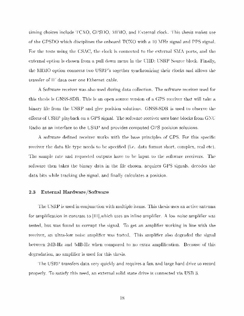
timing choices include TCXO, GPSDO, MIMO, and External clock. This thesis makes use

of the GPSDO which disciplines the onboard TCXO with a 10 MHz signal and PPS signal.

For the tests using the CSAC, the clock is connected to the external SMA ports, and the

external option is chosen from a pull down menu in the UHD: USRP Source block. Finally,

the MIMO option connects two USRP's together synchronizing their clocks and allows the

transfer of IF data over one Ethernet cable.

A Software receiver was also used during data collection. The software receiver used for

this thesis is GNSS-SDR. This is an open source version of a GPS receiver that will take a

binary �le from the USRP and give position solutions. GNSS-SDR is used to observe the

e�ects of USRP playback on a GPS signal. The software receiver uses base blocks from GNU

Radio as an interface to the USRP and provides computed GPS position solutions.

A software de�ned receiver works with the base principles of GPS. For this speci�c

receiver the data �le type needs to be speci�ed (i.e. data format short, complex, real etc).

The sample rate and requested outputs have to be input to the software receivers. The

software then takes the binary data in the �le chosen, acquires GPS signals, decodes the

data bits while tracking the signal, and �nally calculates a position.

2.3 External Hardware/Software

The USRP is used in conjunction with multiple items. This thesis uses an active antenna

for ampli�cation in contrast to [11],which uses an inline ampli�er. A low noise ampli�er was

tested, but was found to corrupt the signal. To get an ampli�er working in line with the

receiver, an ultra-low noise ampli�er was tested. This ampli�er also degraded the signal

between 2dB-Hz and 5dB-Hz when compared to no extra ampli�cation. Because of this

degradation, no ampli�er is used for this thesis.

The USRP transfers data very quickly and requires a fast and large hard drive to record

properly. To satisfy this need, an external solid state drive is connected via USB 3.

18

This thesis relies on the synchronized capture of data. To ensure this, a powered four

way splitter is used. In conjunction with this splitter, a standard Ublox 6 series and a

Novatel Propak v3 are used. The Novatel is chosen because of its ability to capture data

and use information from NTRIP to calculate Narrow Integer RTK solutions. These RTK

solutions are to be used as truth when compared to standard GPS data. A diagram of the

hardware setup is shown in Figure 3.1. The software used for the data collection for the

Novatel is its proprietary software, Novatel Connect. This is a simple GUI that allows one

to see the statistical data real time and capture many di�erent outputs of the receiver. Some

of the outputs include the bestpos option and GPGGA: two of the most highly used data

components in this thesis. The Ublox data on the other hand uses a secondary terminal

software recorder called Putty to capture its data. This allows for the capture of the NMEA

(National Marine Electronics Association) messages naturally output by the Ublox receiver.

For some of the testing with the Ublox the pseudoranges are recorded. This is done with

GoGPS, a free piece of software that will record and output some NMEA messages as well

as raw pseudorange measurements and navigation data in rinex �les.

19

Chapter 3

USRP and GPS Receiver Static Data Research

Chapter three describes how to record and playback static data. All the static data is

captured using the antennas on the roof of the Woltosz Engineering Research Laboratory

at Auburn University. This chapter begins with timing solutions and how clock accuracy

a�ects the GPS position solution. The three clock solutions that are discussed in this section

are mentioned in chapter two. After comparing clocking solutions, the validity of playback

repetition is con�rmed in section three. Finally, lower level measurements are analyzed to

narrow down where the extra error may be coming from.

3.1 Static Testing Comparison Between GPSDO and Internal USRP Clock

The �rst section of chapter three compares two of the three timing options. The two

timing options in this section are TCXO and GPSDO. In this section, the static setup will

be discussed, and the GPSDO is shown to be vastly superior to TCXO timing options.

3.1.1 Static Setup

When designing the static setup, as mentioned in chapter two, the signal has to be split

three or four ways. The signal comes from a Novatel pinwheel down a 90' LMR 400 coax

cable to the powered splitter. The diagram of the setup used for the multiple static datasets

are shown in Figure 3.1. The Novatel, Ublox, USRP, and GPSDO(if used) are connected to

each of the ports. Taking all the data from a single antenna reduces the number of variables

to account for. The Novatel is used to gather the truth position by averaging a narrow integer

solution captured at the same time as the other data sets. This is used in later calculations

and observations.

20

Figure 3.1: Static GPS Hardware Setup

For playback, the GPSDO has to be connected to a GPS antenna (if used) for accurate

timing. The signal that is played back is then run through two 30 dBm attenuators into a

Ublox receiver. Most of the data is captured with the GPSDO excluding one static test and

one dynamic test section. The more accurate clocking changed the errors from 100 meters

to single digit meters of error. Therefor the accurate timing was necessary to make accurate

conclusions about the data that is played back.

All the static data gathered for this thesis was taken at the location shown below

in Figure 3.2. The position averaged from the data is 32.605363880466456 North and -

85.486936035232276 East which is used as truth.

21

Figure 3.2: Data Collection Point for Static Position Analysis

Because the data is gathered by hand, the start time of each data run is di�erent. For

a proper comparison, the data needed to be synchronized. All the �les have UTC time

recorded along with the positions and therefore are parsed according to the UTC time. Each

�le is trimmed to start and end at the same time by hand in post process. Then a script

that is written is used to make sure each iteration matches in time and position, dropping

data points that do not match to keep the time synchronized. Because the static data is

captured at 1Hz, there is no bridge between data rate and actual time.

3.1.2 Static Results without GPSDO

Testing without the GPSDO is done for a complete comparison of position error due to

USRP clock error. While testing, it was observed that the GPS signal dropped quite often.

When processing and plotting the data, seen in Figure 3.3 , the amount of error is notable.

The maximum error in the north direction is 86.4 m error and the error in the east direction

is 92.2 m, but the GPS receiver does not allow continuous drift away from truth. When

recording without the onboard clock disciplined to the OCXO, the error is much worse.

22

With GPS, time is a critical component of the solutions as the di�erence between received

and transmitted signal is vital to the position calculation.

For this static test position data is captured at 1 Hz with the Ublox receiver. Because of

the inaccuracy of Ublox the clock, the played back signal may be o�set slightly from the live

signal. For this, USRP clock accuracy of nanoseconds is necessary. When a TCXO (that is

only accurate to 2.5 ppm) is used, accurate positions will not be collected. Since GPS needs

an accuracy of 0.1 ppm at minimum, the drift of the TCXO causes playback to be o�set

slightly from the true time. This causes the error that is seen in Figure 3.3.

The record and playback is sampled with a lower accuracy clock, but the messages on

the L1 carrier are given with respect to the more accurate GPS time. The positions become

askew during the record and playback functions. With the record and playback seen in

Figure 3.3, part of the problem is possibly due to clock drift in the signal sampling. Now

as the GPS receiver records its positions, it gets time updates, but the time updates do not

take into account the massive USRP clock error.

Figure 3.3 is a graphical representation of the North and East positions, respectively.

The positions from the played back data and the live data have both been subtracted from

truth de�ned earlier; the movement away from the point at each iteration is considered the

error of the receiver.

23

Figure 3.3: Position Di�erenced From Actual Position With Internal USRP Clock

In Figure 3.4 the playback and live data are di�erenced. The data in Figure 3.4 shows

a much more accurate representation of the error caused by the USRP. There is a change in

clock bias for each power cycle of the GPS receiver. The clock bias is assumed to be minimal

in this thesis, so the live and played back GPS signals are handled similarly. Because the

receiver handles live and played back data the same, the position solution should be the

same. This assumes constant clock drift of the GPS receiver used, and therefore the clock

error is di�erenced out.

24

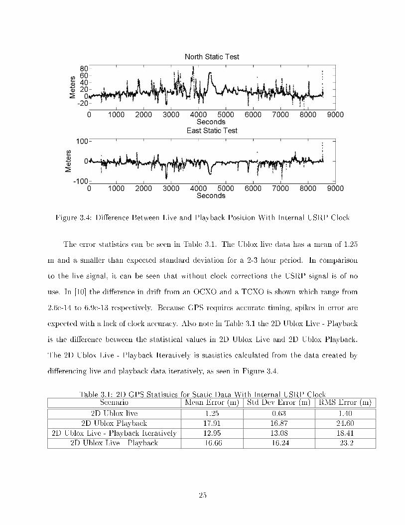
Figure 3.4: Di�erence Between Live and Playback Position With Internal USRP Clock

The error statistics can be seen in Table 3.1. The Ublox live data has a mean of 1.25

m and a smaller than expected standard deviation for a 2-3 hour period. In comparison

to the live signal, it can be seen that without clock corrections the USRP signal is of no

use. In [10] the di�erence in drift from an OCXO and a TCXO is shown which range from

2.6e-14 to 6.9e-13 respectively. Because GPS requires accurate timing, spikes in error are

expected with a lack of clock accuracy. Also note in Table 3.1 the 2D Ublox Live - Playback

is the di�erence between the statistical values in 2D Ublox Live and 2D Ublox Playback.

The 2D Ublox Live - Playback Iteratively is statistics calculated from the data created by

di�erencing live and playback data iteratively, as seen in Figure 3.4.

Table 3.1: 2D GPS Statistics for Static Data With Internal USRP ClockScenario Mean Error (m) Std Dev Error (m) RMS Error (m)

2D Ublox live 1.25 0.63 1.402D Ublox Playback 17.91 16.87 24.60

2D Ublox Live - Playback Iteratively 12.95 13.08 18.412D Ublox Live - Playback -16.66 -16.24 -23.2

25

In this section, it was shown that the USRP onboard TCXO is not accurate enough to

allow for correct record and playback scenarios. Also note that not all the error comes from

the USRP, but it is a culmination of errors that create large error statistics.

3.1.3 Static Results with GPSDO

In this section, the addition of a GPSDO is used. As mentioned earlier, the GPSDO is

GPS disciplined and much more accurate than the TCXO. The GPSDO is approximately

100 times more accurate than the onboard TCXO. Because of this di�erence, the USRP

works much better with the more accurate clock, as shown below in Figure 3.5. Though the

dynamic data is revisited later without the GPSDO, one can see the increase of accuracy is

needed to accurately portray the position data.

Figure 3.5: Static Test With GPSDO

The RTK position is di�erenced from the Ublox position and the position is converted

from degrees into meters to get Figure 3.6. This conversion into meters from degrees is done

with the following parameter: 1degree = 60arc/min 1arc/min = 1852meters. Seen below,

there is a small bias in the north and east direction. In Table 3.1, the mean error gives a

good idea of how much bias there is. This bias is not purely caused by the USRP, but may

include the GPS receiver clock bias.

26

Figure 3.6: Position Di�erenced From Actual Position With GPSDO

The model comparison starts here with the static di�erence of the Ublox position and

the played back Ublox position. As seen in Figure 3.7, there is approximately 6 meters of

total error over all the data which is less that the Ublox or USRP separately. In the north

direction, the max error is 1.6483 m and the minimum is -4.2596 m, making the overall

maximum distance error of 5.9079 m. For the East, the maximum error is 3.1854 m and the

minimum is -1.2408 m making the other over all distance for total maximum error 4.4263 m.

As is shown by geometry, the total maximum error can be calculated using the Equation 3.1

and gives a normalized maximum error of 7.3821 m for the latitude and longitude directions

added by the USRP.

∆xy =√

∆x2 + ∆y2 (3.1)

27

Figure 3.7: Di�erence Between Live and Playback Position With GPSDO

In an attempt to look for speci�c frequencies and other patterns in the error, the spectral

density was taken of the data. One thing that is observable between the recorded and played

back data, is the drop in power during playback of approximately 4dB/rad/s. There were

no other di�erences noticed in the spectral content are the errors as shown in Figure 3.8.

Figure 3.8: Static Live vs Playback PSD of Position

During the test with the GPSDO, the carrier to noise ratio measurements were cap-

tured. These measurements are a good guide for the strength of GPS signal from individual

satellites. The lower the carrier to noise ratio is, the worse the signal is overall. The carrier

28

to noise is slightly di�erent between live and playback, seen in Figure 3.9. To get a better

look at the changes caused by the USRP, the live and played back carrier to noise signals

are di�erenced and shown in Figure 3.10. These tables show that when clocking is accurate

enough the signal is not heavily degraded.

Figure 3.9: Comparison of C/No with GPSDO with GPS

Figure 3.10: Di�erenced of C/No with GPSDO with GPS

3.1.4 Statistics with GPSDO

In this section, the statistics of the data collected and played back using the GPSDO

will be discussed. The main statistics calculated from this data are shown in the two tables

below. Table 3.2 is a table of the statistics calculated on latitude and longitude individually.

Altitude is not used in this thesis, because the height error is least important when dealing

29

with ground vehicles. As can be seen, the USRP does add error to the position solutions,

but it is at a magnitude that does not invalidate the data that is played back.

Table 3.2: Latitude and Longitude GPS Statistics for Static Data with GPSDOScenario Mean Error (m) Std Dev Error (m) RMS Error (m)

Lat Ublox live 1.16 .61 1.32Lat Ublox Playback 2.12 1.07 2.37

Lat Ublox Live-Playback Iteratively -0.96 0.88 1.30Long Ublox live .56 .76 .95

Long Ublox Playback -.38 1.05 1.08Long Ublox Live-Playback Iteratively 0.94 0.70 1.18

Because latitude and longitude are considered the most important measurement in this

study, below is a table of this 2D statistical analysis. When looking at the two dimensional

statistics it is easier to get a more cumulative idea of the errors. In Table 3.3 it can be seen

that the mean is not zero for the Ublox and USRP di�erence. The standard deviation and

RMS error does increase, but both increase less than 1 meter. This is less than 1/3 of the

overall error of GPS.

Table 3.3: 2D GPS Statistics for Static Data with GPSDO2D Scenario Mean Error (m) Std Dev Error (m) RMS Error (m)

Ublox live 1.53 0.54 1.62Ublox Playback 2.39 1.05 2.61

Ublox Live-Playback Iteratively 1.05 0.77 1.30Ublox Live-Playback -.86 -.51 -.99

3.1.5 Static Conclusions with and without GPSDO

It is clear from the static data that a GPSDO is required to get acceptable data for

USRP playback. The error itself comes from two di�erent sources between the live and

played back data. The error comes from both the USRP and the Ublox receiver for the

played back data. The USRP inserts noise during the process of record and playback from

its high noise �oor and the clock error. In addition to the USRP adding error during record,

it does the same during playback. There is also error from the Ublox receiver clock, and

30

even though it is the same data processed the same way by the same receiver, the clock drift

still exists and changes the position error.

3.2 CSAC Timing

3.2.1 Background

In Section 3.1 the basic need of accurate timing for the USRP was discussed. Thus far,

two methods of timing have been used. The �rst method was using a TCXO, this is very

inaccurate and the error was shown to be unacceptable. The GPSDO was then used, and the

standard deviations decreased from 20m to 2m. The third method, timing with the CSAC,

will be discussed in this section.

3.2.2 Hardware Setup

When setting up the CSAC, a few changes are needed. First, the USRP cannot have a

GPSDO attached to it internally; if it does the GPSDO will take precedence and the USRP

will not use the external clock reference. Second, the CSAC needs to output both a 10 MHz

clock signal and a 1 PPS signal. The 10 MHz signal disciplines the on board TCXO and

the PPS tells the USRP when to start the data collection. The CSAC requires about 15

minutes to stabilize [1], so for this test the CSAC is turned on 15 minutes prior to any data

recording. The whole USRP setup can be seen in Figure 3.11.

31

Figure 3.11: Static Hardware Setup with CSAC

3.2.3 Results

Because the USRP with the GPSDO has timing that is disciplined by GPS, the CSAC

playback is expected to perform about the same as the data taken with the GPSDO. As is

seen in Figure 3.12, the playback data of the Live and playback Ublox and Novatel RTK,

looks much closer to the live Ublox than in Figure 3.5. After the �rst 500 seconds, the

positions settle and are almost plotted right on top of each other.

Figure 3.12: North and East Position with CSAC

32

Because of the position change seen in Figure 3.12, the data run is split into a start

and �nish section. During the live data set, the Ublox is running approximately 10 minutes

before the data collection was started. On the other hand the GPS receiver starts providing

position solutions as soon as playback starts creating the settling period seen in Figure 3.13.

This settling period was visually determined to be �nished at 500 seconds as seen in Figure

3.13. Because the receiver is starting from a cold start, the �lters have to converge to the

best position possible, and this happens around second 500. Because of the time the position

takes to settle, the USRP should not be used for extremely short datasets.

Figure 3.13: First 500 Seconds of Playback with CSAC

The position di�erenced from the known position continues in Figure 3.14 and shows

how close the two data sets are. The separation between both data sets is much smaller than

in Figure 3.6, graphically showing the improvement caused by the CSAC.

33

Figure 3.14: After First 500 Seconds of Playback with CSAC

The live and played back datasets are di�erenced again in Figure 3.15. In this �gure,

the bias is quite more signi�cant than the noise. This error would not be characterized as a

random walk, but is instead closer to a bias with white noise.

Figure 3.15: Live and Playback Di�erenced with CSAC

The PSD of the CSAC data is not much di�erent from the static data with the GPSDO.

Again in Figure 3.16, there are no additional frequencies added just like in the static data

with the GPSDO.

34

Figure 3.16: Live vs Playback PSD of Position with CSAC

3.2.4 Statistics

The statistics of the CSAC data are given in Table 3.4. There is still a bias, but the

standard deviation is relatively small when looking at the di�erence between live and play-

back data. The statistics using the CSAC are better than the statistics using the GPSDO.

The increased accuracy caused by the CSAC was not expected because the accuracy of

the GPSDO is GPS disciplined. The CSAC is most likely more accurate because of the

compounding of clock errors with record and playback.

Table 3.4: CSAC Record and Playback DataScenario (2D) Mean Error (m) Std Dev Error (m) RMS Error (m)

Ublox live 1.60 .65 1.73Ublox Playback 2.02 .72 2.14

Ublox Live-Playback Iteratively -.42 0.72 .83Ublox Live-Playback -.42 -.07 -.41

3.2.5 Conclusions

As can be seen from the data after an initial settling period; the live and playback data

are similar. In Table 3.5, the CSAC and standard GPSDO error are compared.

35

Table 3.5: CSAC Compared to Static with GPSDOScenario Mean Error (m) Std Dev Error (m) RMS Error (m)

2D Ublox Live-Playback CSAC -.42 -.07 -.412D Ublox Live-Playback GPSDO -.86 -.51 -.99

CSAC-GPSDO .44 .44 .58

The standard deviation and RMS errors show that the CSAC recorded positions have

signi�cantly better position solutions. These statistics both show the CSAC to be far superior

when logging data. The CSAC has much lower clock drift and is more accurate than the

GPSDO with the GPS time updates. The CSAC is more di�cult to use, but from these

tests it is worth it to use the CSAC over other clocking methods.

3.3 Repeatability of Record and Playback with the USRP N210

3.3.1 GPSDO GPS vs Non-GPS

Repeatability is an important consideration when using the USRP to record and play-

back. If the USRP is not repeatable the testing of multiple receivers would not be a viable

option. The testing plan includes playing back one data set 11 times. This was done over

multiple days as the individual data sets were two hours long.

For the data run that is shown in Figure 3.17 seven out of the eleven data runs were

done with the aid of GPS for the GPSDO. The other four runs were done without the aid of

GPS. The four runs without GPS were done to see the signi�cance of GPS disciplined clock.

In Figure 3.17 the left top and bottom data runs are the ones recorded with the aid of GPS,

while on the right top and bottom are the data runs without GPS aided timing. As can be

seen the data without the GPS aided timing drifted signi�cantly.

36

Figure 3.17: Repeatability Test With and Without GPS Aided GPSDO Timing

3.3.2 Repeatability Di�erences

After recording the �rst data sets more evaluation was required. In this section a better

comparison is made between each playback cycle. For this di�erencing test, the �rst four

runs of the previous test were used. Figure 3.18 show plots di�erencing the �rst four runs

from Figure 3.17. This is to see the di�erence in error between each playback dataset. In

Figure 3.18 the two plots on the left are the �rst Ublox data structure di�erenced from the

other three. The plots on the right are the rest of the data di�erenced from each other. From

these graphs the di�erence between each run can be observed, but a clearer picture can be

seen with the calculated statistics.

37

Figure 3.18: Repeatability Test Di�erenced

3.3.3 Statistics

The statistics from the repeatability test in Figure 3.18 are shown below in Table 3.6.

These calculations are of the normalized latitude and longitude, and therefore are the two

dimensional data from the di�erence between the runs.

Table 3.6: Error Statistics for RepeatabilityScenario Mean Error (m) Std Dev Error (m) RMS Error (m)

Live 1.18 0.61 1.33Playback 1 1.63 0.94 1.88Playback 2 1.59 0.94 1.84Playback 3 1.60 0.95 1.86Playback 4 1.59 0.93 1.85Playback 1-2 0.041 0.003 0.037Playback 1-3 0.030 -0.002 0.025Playback 1-4 0.036 0.010 0.036Playback 2-3 -0.011 -0.006 -0.012Playback 2-4 -0.005 0.007 -0.001Playback 3-4 0.006 0.011 0.011

Playback 1-2 Iteratively 0.33 0.18 0.38Playback 1-3 Iteratively 0.31 0.18 0.36Playback 1-4 Iteratively 0.24 0.15 0.28Playback 2-3 Iteratively 0.14 0.08 0.16Playback 2-4 Iteratively 0.22 0.13 0.26Playback 3-4 Iteratively 0.20 0.12 0.23

38

3.3.4 Repeatability Between Receivers

One of the goals of writing this thesis is to show how the data from the USRP can be

used to evaluate di�erent receivers. To do this, two completely di�erent types of receivers are

compared in both live and playback scenarios to show whether the testing is repeatable in

comparing receivers. The two receivers chosen for their separate methods of signal processing,

were the Ublox EVK 6T and the Novatel OEM V3. While running this test a higher sample

rate of 10Ms/s was required compared to the 5Ms/s used in the rest of the paper. This was

to satisfy the Novatel receiver requiring a higher quality signal.

3.3.4.1 Results

The played back signal is run from the USRP through a splitter to both Ublox and

Novatel receivers. The Novatel GPGGA measurements are compared to the Ublox data in

Figure 3.19. Di�erent receivers react di�erently to errors and this test will show how these

two receivers react to the errors created by the USRP. It can be seen in Figure 3.19, that the

Novatel �lters the data much more than the Ublox receiver, and this shows that the errors

created by the USRP do not have the same e�ect on the Novatel as on the Ublox.

Figure 3.19: Repeatability Test Di�erenced

39

From this data the statistics below in Table 3.7 is extracted. With this speci�c data

set, the Novatel did not calculate a better position than the Ublox. However, the USRP

playback signal did e�ect both receivers in approximately the same way.

Table 3.7: 2D GPS Statistics for Static Data with GPSDO2D Scenario Mean Error (m) Std Dev Error (m) RMS Error (m)

Ublox live 1.09 .33 1.1Ublox Playback 1.39 .68 1.55Novatel Live 1.65 .49 1.72

Novatel Playback 1.58 .96 1.85

3.3.5 Conclusions

In this section the repeatability of the USRP was discussed with a standard GPSDO,

which can be purchased with the USRP. For this testing a few conclusions can be made.

First, the USRP must have GPS data sent to the GPSDO for accurate playback. Record

and playback can be accomplished without GPS-aided GPSDO, but the data is slightly more

accurate when using GPS aided timing. The di�erence between the playback data sets are

quite small, making them very repeatable. Overall, this test shows the viability of the USRP

for playing back the same data multiple times. While testing the cross platform uses of the

USRP, the data shows that the extra errors created by the USRP a�ects di�erent receivers

in approximately the same way with slight di�erences. This means that di�erent receivers

can be tested from one data set using the USRP.

3.4 Pseudorange and Lower Level Measurements

In this section, the pseudorange measurements are analyzed. Errors on these measure-

ments have a direct correlation to the error in position. This section will statistically analyze

the errors on pseudorange, doppler, and C/No measurements.

40

3.4.1 Background Work

The pseudorange is the range between satellite and with additional errors. In the pseu-

doranges, there are inherent errors shown in Equation (3.2).

ρ = r + cdtr + +eA + cdtUSRP + σUSRP + σ (3.2)

In this equation, r is the absolute range between satellite and user, eA is the atmospheric

error including troposphere and ionosphere, cdte is the receiver clock error, σUSRP is the

thermal noise error caused by the USRP, cdtUSRP is the clock error created by the USRP,

and σ is the rest of the errors including the satellite clock error, white noise and other small

errors.

The GoGPS software mentioned earlier, takes raw messages from the Ublox receiver and

outputs multiple rinex �les which can be processed later to gather pseudoranges, doppler,

C/No, ephemeris, and more.

This section seeks to discover if during the two runs the same pseudorange data is being

received during record and playback. Because the USRP records IF data at such a high

rate, theoretically there should be minimal changes in the pseudoranges from record and

playback through the USRP. Therefore only a minimal amount of error is expected between

pseudorange lengths. According to the results, however, this is not the case.

3.4.2 Results

The �rst measurement type observed is the pseudorange. In Figure 3.20 the pseudor-

anges from live data are compared to playback. This �gure veri�es that good pseudorange

data has been recorded for this data set (by showing there are no extreme measurement

changes).

41

Figure 3.20: Pseudorange Measurements Live and Playback

To start looking at the changes between the recorded and played back data the time

vectors are synchronized and the ranges are di�erenced. Each live satellite is di�erenced from

its respective playback satellite. This is done and the result are shown in Figure 3.21, where

the overall change in meters is extremely large. The error for each pseudorange measurement

is extremely large expressing a possible large clock error term in the calculations. When

observing the data points at one speci�c time; the measurements do not have a large change

between pseudoranges. The error between pseudoranges at one time stamp can be seen in

Figure 3.22 showing the measurement for each satellite at this time stamp. Figure 3.22 is

the same plot as 3.21 zoomed into one speci�c point with a legend. The maximum di�erence

between these measurements is two meters.

42

Figure 3.21: All Pseudoranges Di�erenced 13SVs

Figure 3.22: Enhanced Di�erence Between Pseudorange Measurements 13SVs

Figure 3.23 is a comparison of two satellites chosen for their longevity. These two

satellites are both in the complete data set. Looking at the two satellites separately gives a

much better idea of what error is being created by the USRP. The ranges are di�erenced with

respect to time in the graphs on the right of Figure 3.23. This is done to see the change in

pseudorange between each measurement which shows the position change of the individual

satellite. In both di�erenced pseudorange �les, the pseudoranges have a constant change in

position from the live data. On the other hand, the playback data always starts o�set and

43

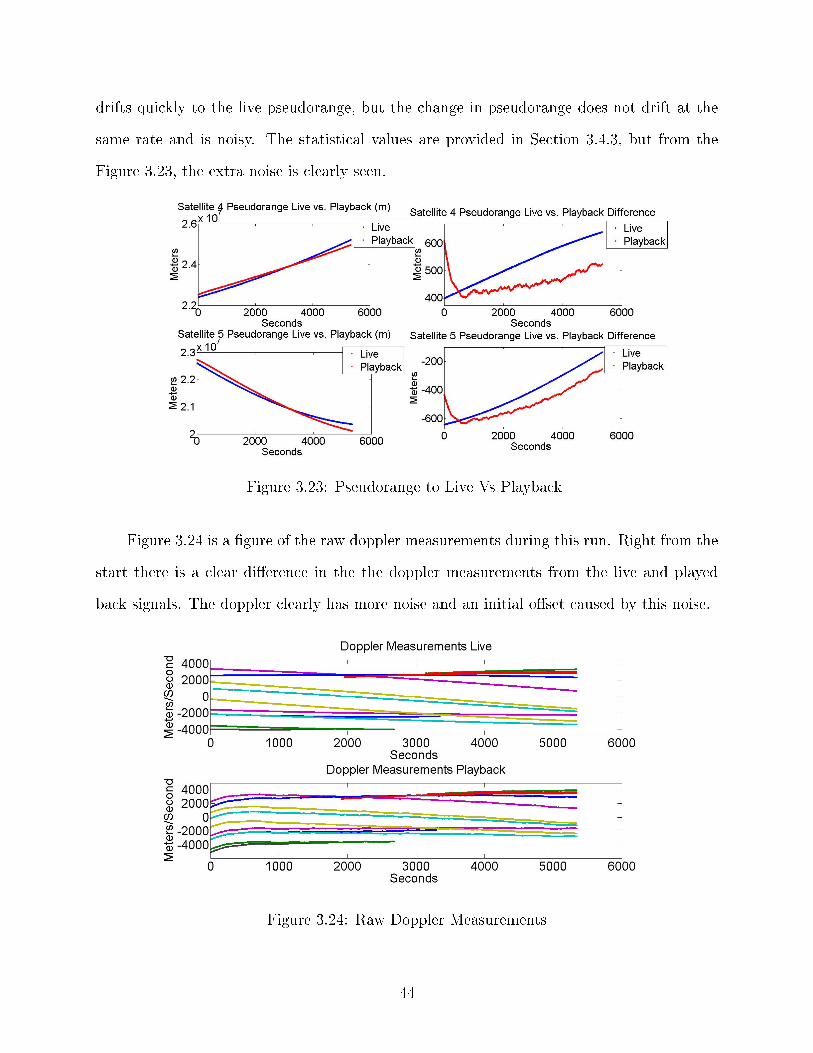
drifts quickly to the live pseudorange, but the change in pseudorange does not drift at the

same rate and is noisy. The statistical values are provided in Section 3.4.3, but from the

Figure 3.23, the extra noise is clearly seen.

Figure 3.23: Pseudorange to Live Vs Playback

Figure 3.24 is a �gure of the raw doppler measurements during this run. Right from the

start there is a clear di�erence in the the doppler measurements from the live and played

back signals. The doppler clearly has more noise and an initial o�set caused by this noise.

Figure 3.24: Raw Doppler Measurements

44

The doppler is then di�erenced, and just like the pseudoranges. The doppler shows

a large change in magnitude of meters per second. Figure 3.25 uses the same di�erencing

method used for the pseudorange measurements. As can be seen, there is a large error at the

start, and the measurements are very noisy. This demonstrates that the same error source

e�ects in the pseudoranges is also e�ect the doppler.

Figure 3.25: All Di�erenced Doppler Measurements

As shown earlier in the pseudorange section, satellites four and �ve are singled out for

their continuous data. The doppler measurements on satellites four and �ve are signi�cantly

di�erent between the live and playback data. The noise and drift of the playback data

is signi�cantly di�erent between the two measurements seen in Figure 3.26. When the

measurements are di�erenced in time, observe that the noise during playback is signi�cantly

higher. From what is seen in Figure 3.25 and 3.26, it can be concluded that the error here

is clock noise. This is not quanti�ed, but it is obvious that the error on the doppler is

signi�cantly large.

45

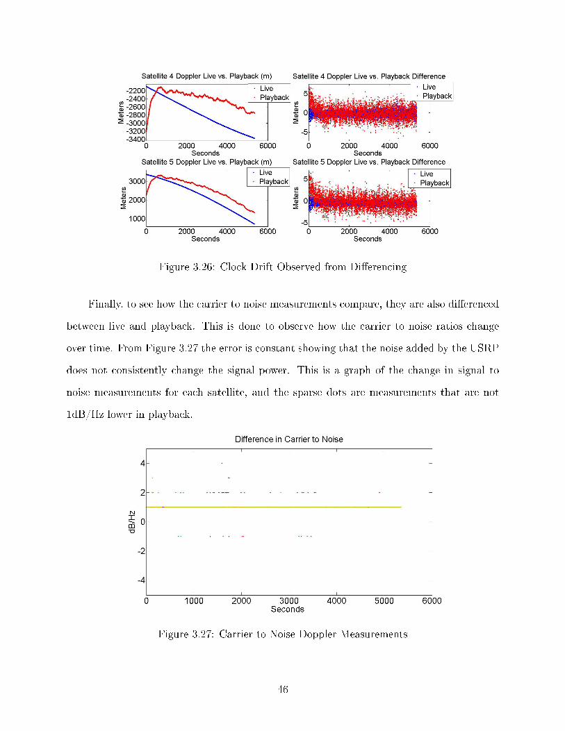
Figure 3.26: Clock Drift Observed from Di�erencing

Finally, to see how the carrier to noise measurements compare, they are also di�erenced

between live and playback. This is done to observe how the carrier to noise ratios change

over time. From Figure 3.27 the error is constant showing that the noise added by the USRP

does not consistently change the signal power. This is a graph of the change in signal to

noise measurements for each satellite, and the sparse dots are measurements that are not

1dB/Hz lower in playback.

Figure 3.27: Carrier to Noise Doppler Measurements

46

3.4.3 Statistics

To get a more comprehensive overview of statistics, satellites four and �ve are used for

their length and continuity. The time di�erenced data is used to see how the measurements

change statistically over time. From Tables 3.4.3 and 3.4.3 it is easily observed, that there

is a signi�cant amount of extra error on both the pseudoranges and the doppler created by

the USRP.

Table 3.8: Pseudorange StatisticsScenario Mean Error (m) Std Dev Error (m) RMS Error (m)

Satellite 4 Live 527.20 71.53 532.03Satellite 4 Playback -421.75 149.80 447.56Satellite 5 Live 457.87 36.63 459.33

Satellite 5 Playback -491.08 108.62 502.95

Table 3.9: Doppler Di�erence StatisticsScenario Mean Error (m) Std Dev Error (m) RMS Error (m)

Satellite 4 Live -.24 .68 .72Satellite 4 Playback -.50 .43 .66Satellite 5 Live .08 1.69 1.70

Satellite 5 Playback -.17 1.61 1.62

3.4.4 Conclusions

From this section the errors from the USRP have been further investigated. The USRP

adds large error in position due to the low quality clock. The error seen in the pseudoranges

and doppler due to the USRP recording was also seen to be very large. However the extra

error seen is similar along each satellite such that good positions are calculated by the GPS

receiver in playback.

47

Chapter 4

Dynamic Testing

In this chapter, dynamic data is gathered and discussed. This is split into three data

sets: Dynamic without GPSDO, Dynamic with GPSDO, and High Dynamic with GPSDO.

Both standard dynamic sets are recorded around a large circular road to keep the data as

smooth as possible. The High Dynamic data set is taken on a much smaller track so that

speed can be regulated allowing for much faster speeds which show higher dynamic properties

of the USRP.

4.1 Data gathered

When recording the dynamic data, the hardware setup is similar to the static data. One

di�erence between static setup and dynamic setup is the use of a mobile wireless connection

for NTRIP corrections, and a stable power source. NTRIP is a piece of software that uses

data from a local base station via the internet for RTK corrections. The dynamic tests also

use a coax cable that is approximately 80' shorter than used for the static testing. The

vehicle used for the dynamic data gathering was an In�nity G35 seen in Figure 4.2. This

vehicle has no such power stability problems. The data taken for the dynamic testing is

taken around the path shown in Figure 4.1.

48

Figure 4.1: Dynamic Path

As can be seen in Figure 4.1, the data is taken on a road, and therefore standard

driving practices were observed. To keep the data as uniform as possible, acceleration and

deceleration is kept to a minimum.

49

Figure 4.2: Vehicle Used for Dynamic Test Data collection

4.1.1 Dynamic Data Analysis Using internal USRP clock

To compare to the static data, the �rst set of analysis for dynamic testing uses the

internal USRP clock (i.e no GPSDO). This section shows the comparison of statistics between

static and dynamic data using the USRP. It is observed in Figure 4.3, that the error spikes

are much larger than the static data seen in Figure 3.3.

50

Figure 4.3: Dynamic Position Di�erenced From Actual Position With Internal USRP Clock

Figure 4.4 shows the amount of error the USRP adds to the dynamic signal in playback.

There are multiple position spikes that are much greater than the static set. To compare

static and dynamic statistics most accurately, the data is tabulated together in Table 4.1.

The largest of these spikes are in Table 4.2 to quantify the magnitude of the error spikes. As

seen in this table the GPS receiver reacts to dynamic and static playback data di�erently.

51

Figure 4.4: Dynamic Di�erence Between Live and Playback Position With Internal USRPClock

Table 4.1: 2D GPS Statistics for Data with no GPSDOScenario Mean Error (m) Std Dev Error (m) RMS Error (m)

2D Static Ublox live 1.53 0.54 1.622D Static Ublox Playback 2.39 1.05 2.61

2D Static Ublox Live-Playback -.86 -.51 -.992D Dynamic Ublox live 4.87 28.04 28.46

2D Dynamic Ublox Playback 27.28 39.00 47.592D Dynamic Ublox Live-Playback 18.61 24.99 31.16

Table 4.2: Maximum Error Spikes Caused by USRP without GPSDOScenario Position Error North (m) Position Error East (m)

Static Data 86.4 92.2Dynamic Data 268 631

A better understanding of the carrier to noise error can be found with the dynamic

data. In the �gures below the carrier to noise is averaged for each satellite shown. Figure

4.5 shows the comparison of record and playback. Figure 4.6 shows the change in C/No

measurements. The carrier to noise ration changes 5.5 dB-Hz maximum and is compared to

data with the GPSDO in Section 4.1.2.

52

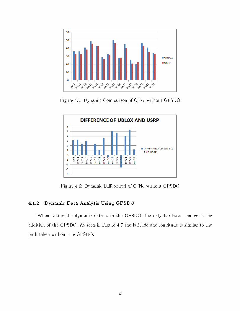
Figure 4.5: Dynamic Comparison of C/No without GPSDO

Figure 4.6: Dynamic Di�erenced of C/No without GPSDO

4.1.2 Dynamic Data Analysis Using GPSDO

When taking the dynamic data with the GPSDO, the only hardware change is the

addition of the GPSDO. As seen in Figure 4.7 the latitude and longitude is similar to the

path taken without the GPSDO.

53

Figure 4.7: Dynamic Test With GPSDO

To get the error of the Ublox receiver the RTK position is needed for each time stamp.

To run statistics on this error the Ublox data is di�erenced from the Novatel data seen in

Figure 4.8. When the data was originally taken, the dynamic data with use of the GPSDO

had large errors due to corrupted internet connection for the Novatel. Therefore these data

points were removed as seen in Figure 4.8.

Figure 4.8: Dynamic Position Di�erenced From Actual Position With GPSDO

Figure 4.9 is a result of di�erencing live and playback for the dynamic data with the

GPSDO. With a simple visual comparison between Figures 4.9 and 3.7 it can be seen that

54

dynamics add extra error to the playback. The error statistics are provided later in Section

4.1.3.

Figure 4.9: Dynamic Di�erence Between Live and Playback Position With GPSDO

Additionally, the PSD (Power Spectral Density) pro�le of the position solutions are

di�erent between live and playback data. As seen in Figure 4.10, the USRP has a smoothing

a�ect to the error frequency. This smoothing is a result of the sampling process.

Figure 4.10: Dynamic Live vs Playback PSD of Position

55

In the �gures below, the carrier to noise is provided for the dynamic data using the

GPSDO. In this section an actual comparison between carrier to noise measurements taken

with and without the GPSDO can be made. In Figure 4.6 the maximum carrier loss is around

5.5dB-Hz, while the measurements seen in Figure 4.12 has a max loss around 1.75dB-Hz.

This comparison shows the magnitude of noise added to the GPS signal with and without

the GPSDO.

Figure 4.11: Dynamic Comparison of C/No with GPSDO

Figure 4.12: Dynamic Di�erenced of C/No with GPSDO

4.1.2.1 High Dynamic Testing

After observing how the dynamic runs di�ered from the static runs, the following ques-

tion was proposed: How is dynamics correlated to error in Record and Playback created by

56

the USRP? In this section, higher dynamic data will be compared to lower dynamics for any

correlation between speed and accuracy of USRP.

High Dynamic Setup The high dynamic data set starts with one one minute of stationary

data for a baseline. Then the vehicle drives along the path shown in Figure 4.13. This

location is chosen because it is a nice controlled path that multiple tests can be conducted.

This data is also calculated at 5 Hz because it is a much shorter data set.

Figure 4.13: High Dynamic Path

The data is taken in three di�erent ways. First run was recorded at at 65 mph, this

data was taken while driving 2-3 times around the track. The second test was recorded at

45 mph, which was also driven 2-3 times around the track. The �nal test was a high speed

J turn to observe the sudden drift of the Ublox receiver.

High Dynamic Results The 2D plot of the path taken is shown in Figure 4.14.

This shows the high dynamic path as well as, where the data was taken on the skid pad and

demonstrates the controlled environment used for the J turn.

57

Figure 4.14: High Dynamic 2D Position with All 3

The data from the high dynamic tests will be split into statistical analysis for each

of the three scenarios mentioned in setup. This will also only be done for the di�erence

between record and playback. Figure 4.15 is the graphical representation of live and playback

di�erenced. There are clear patterns derived from this speci�c data set and easily seen in

the Figure 4.15. When running the statistics on the high dynamic data, the data was run

individually by the three separate tests. As mentioned earlier the data set starts stationary

and then goes to 65 mph for 430 seconds around the track. The vehicle then slows to 45

mph from second 431 to 900, and after getting in position multiple J turns were conducted

between seconds 1140 till the end. Each part of the run can be seen here in Figure 4.15.

These are separated in Figure 4.15 by dashed lines and tabulated in Table 4.5 in the statistics

section below.

58

Figure 4.15: High Dynamic Ublox Live vs Ublox Playback

4.1.3 Statistics

The statistics in this section are gathered from dynamic data with the use of a GPSDO.

Table 4.4 shows how the USRP performs with dynamic data. This can be compared to

static data, and it is concluded that the USRP corrupts the dynamic data more than static.

However this data does not quantify how e�ective the USRP is with all dynamic data.

When looking at the statistics for the data captured with the GPSDO, the data is split

into two tables seen below. Table 4.3 shows the individual latitude and longitude errors.

The data in 4.3 and 3.2 can be compared showing an error increase with dynamic data with

the USRP. Table 4.4 shows the overall error for the 2D position solution.

Table 4.3: Latitude and Longitude GPS Statistics for Dynamic Data with GPSDOScenario Mean Error (m) Std Dev Error (m) RMS Error (m)

Lat Ublox live .93 1.39 1.67Lat Ublox Playback .98 2.22 2.42

Lat Ublox Live-Playback -.05 -.82 -.75Long Ublox live .8 1.55 1.74

Long Ublox Playback .69 2.45 2.55Long Ublox Live-Playback .1 -.91 -.81

59

Table 4.4: 2D GPS Statistics for Dynamic Data with GPSDOScenario Mean Error (m) Std Dev Error (m) RMS Error (m)

2D Ublox live 2.02 1.32 2.412D Ublox Playback 2.97 1.86 3.52

2D Ublox Live-Playback -.96 -.54 -1.12D Ublox Live-Playback Iterative .99 .75 1.24

In Table 4.5 the statistics of the high dynamic data sets are separated out into their

individual sections. This table shows how dynamics a�ect the USRP during record and

playback. As can be seen from this table the USRP error is correlated to the speed of the

vehicle. The data in the �rst two rows of Table 4.5 is fairly conclusive because it represents

many types of data. However conclusive the data from the J turns is not because the short

amount of data taken.

Table 4.5: High Dynamic StatisticsScenario Mean Error (m) Std Dev Error (m) RMS Error (m)

Data Run at 65 MPH 1.87 .74 2.01Data Run at 45 MPH .90 .66 1.12

J turns 2.01 1.12 .94

4.2 Dynamic Conclusions

The dynamic data started with data taken with the internal USRP clock. This data

again con�rmed the need for the GPSDO and shows how much of a change dynamic situations

create for record and playback with the USRP. The GPSDO is then used to give a better

USRP performance. This data is comparable to the static data taken with the GPSDO. The

carrier to noise ratio is also compared with and without the GPSDO, showing signi�cant

noise is added to the signal due to the USRP clock. The RMS error increases by over 30%

changing from static to dynamic data.

High dynamic data is taken to see if there is a correlation between speed and error from

the USRP. From the high dynamic data, the faster the USRP moves when recording data

the more noise speci�cally created by the USRP. This characteristic can be seen in Figure

60

4.15 and Table 4.5. Both show that there is a correlation, although the correlation is not

quanti�ed in this thesis.

61

Chapter 5

Analysis of USRP Record and Playback Using a Software Receiver

This chapter covers the general workings of a software receiver and how the GNSS-SDR

receiver [9] is used to collect data. The error added by the USRP record and playback to

the position using the GNSS-SDR software receiver is discussed. It will also cover many of

the issues of using a software receiver, instead of a hardware receiver. Two software receivers

were considered for this thesis, and the �nal decision of using the GNSS-SDR over the Akos

receiver will be explained.

5.1 GPS Software Receiver Background

5.1.1 How receivers work in general

The software receiver takes a binary IF �le, parses the data, and extracts the data bits

from the IF data. To extract bits out of the IF �le certain information must be known includ-

ing: the sampling frequency, IF frequency, data type, etc. Once this and other information is

known, the IF data is multiplied by the gold code for each satellite to acquire the signal. The

bits are originally placed on the carrier by BPSK which phase modulates the carrier. This

means if a data bit is transmitted the carrier phase is �ipped. For instance, if the phase was

90 it would switch to -90 showing a bit transition. This method is used instead of frequency

or amplitude modulation so that one frequency can carry all the satellites data. The entire

1023 bits of the gold code are placed in 1 ms of data, and one bit of the data message comes

across about every 20 Ms. This is all done on the L1 carrier signal. To acquire a satellite,

the signal needs to be multiplied by the gold code for each satellite and each chip; while the

Doppler is simultaneously scanned for the best Doppler frequency. This is shown in Figure

5.1 where this �spike� denotes what Doppler and what bit of the gold code the signal is on.

62

Figure 5.1 is a graphical representation of acquisition. There are two methods of acquisition,

series and parallel. This thesis shows the series method in Figure 5.1.

Figure 5.1: Series Acquisition

As can be seen in Figure 5.1 there is some noise around the spike. Depending on the

location and signal strength, there may be enough noise to make the �spike� indistinguishable

by the code. If the satellite is indistinguishable from the noise the satellite will not be

acquired. If this is an issue due to RF noise or other external circumstances, the integration

time can be increased to make the �spike� more prominent. This is done in Figure 5.2 using

a 10ms integration period to show the di�erence.

Figure 5.2: Series Acquisition 10Ms

63

Serial acquisition is a time consuming method of acquisition. A faster method is the

parallel search method. Using a parallel method, the entire constellation can be acquired in

about half the time that one satellite can be done in serial acquisition. The parallel method

is however used by the GNSS-SDR for acquisition.

Once a satellite is acquired, the data bits can be extracted for information about the

satellites. The message is transmitted at a much slower rate than the PRN code, so after the

signal is acquired the preamble (start) navigation message is searched for, and each subframe

starts with the string of bits called the preamble. Figure 5.3 from [2] is a representation of

the 5 subframes for the GPS Navigation Data message. The �rst three subframes contain

the ephemeris data and the last two contain the almanac. The almanac is transmitted in

24 separate frames in subframe 4 and 5. This takes approximately 12.5 minutes because

of the amount of data received. It takes between 18 and 30 seconds to acquire a satellite,

because it takes 6 seconds to receive each subframe. If the receiver does not start tracking

the satellite at the start of the �rst subframe it will take the full 30 seconds. Each receiver

can also lose signal, but store the individual subframes making tracking faster when the

signal is reacquired. The only data required to start decoding satellite information comes in

the ephemeris subframes. A complete GPS position can be calculated with ephemeris and

pseudoranges of four satellites .

64

Figure 5.3: Sub Frames of GPS Ephemeris Message[2]

5.2 Software Receiver Selection

There were two software receivers considered for use in this thesis. The �rst one dis-

cussed, which is not used, is a receiver based o� the software receiver in the book [3]. The

Akos receiver code is written in Matlab with a large source of the code derived from code

provided in the Akos book [3]. It is set up to take binary data in Matlab chip by chip to

acquire and track GPS signal using a standard PLL loop. This receiver was modi�ed to use

the receiver to track satellites with USRP data. The modi�ed version parses the code slightly

di�erent and can be tuned for better tracking. This receiver can acquire many satellites with

high C/No measurements, but only 2 satellites were tracked with data used for this thesis.

With the Akos receiver, it is simple to make changes at any point in the receiver.

65

The receiver chosen for the work in this thesis is the GNSS-SDR. The GNSS-SDR

receiver is an open source receiver created to work with GNU Radio. It was not designed

speci�cally for use with the USRP, but GNSS-SDR is used often with the USRP interface.

With this receiver the writers of the code advise to make changes only to the con�guration

�les. This does not give complete control over the receiver but is acceptable for this thesis.

Because the code is written in C++ and designed to use GNU Radio manipulating the base

code was not advised by the code writers. This receiver outputs positions, time, carrier to

noise and more if requested.

GNSS-SDR is chosen to test the record vs playback abilities of the USRP for its interface

simplicity. Though the Akos receiver is simpler to change, there were issues with parsing the

data properly making it less desirable. The GNSS-SDR was made to work with the USRP

and was therefore chosen.

5.3 Drawbacks

There are some drawbacks to using software receivers. Though the software receiver may

have the capability to be tuned for speci�c scenarios quickly; to receive multiple data types

major changes need to be made. While using the GNSS-SDR receiver, two di�erent �les are

used. One is data captured as 2 bit binary and the other is 32 bit complex �oat solutions.

Because the receiver is programmed for 32 bit complex �oat solutions the receiver could not

use the 2 bit data. Another issue is the software receiver �lter. A software �lter does not run

as fast as a hardware �lter that is in most hardware receivers. Finally, one large issue with

the software receiver is slight o�sets in timing. This receiver can not use data captured with

a GPSDO because of the increased clocking accuracy. GNSS-SDR was designed to work

with GNU radio, but does not have a clocking type choice in the con�guration �le. This

forced the data to be capture and used without the increased accuracy of the GPSDO.

66

5.4 Software Receiver Uses

This thesis focuses on the USRP's ability to record and playback GPS data. Even

when dealing with the pseudoranges, the GPS signal was played back into the Ublox. In

this section, the error from the recording process are isolated during the recording process,

and eliminating the errors induced through the playback. The intention is to get position

solutions from the IF data and compare those to the known position. The data recorded and

shown in the results were recorded without a GPSDO and therefore can only be compared

to data without the GPSDO. The position is compared to the truth position of the antenna

on the roof of the Advanced Research Lab mentioned in Section 3.1.1.

5.5 Results From the Software Receivers

This data shows how the GNSS-SDR receiver deals with the error caused by the USRP.

During testing many issues were discovered. While debugging these issues the inline ampli�er

was revisited. Figure 5.4 con�rms the ampli�cation does not need to be used by showing

the magnitude of extra noise added by an inline ampli�er in this test setup.

Figure 5.4: Live Software Receiver Data with and Without ampli�er

67

The software receiver has multiple large spikes in position error without ampli�cation.

These spikes are short in duration and create havoc in the statistics. Because of this, there

are three comparisons made here when looking at this data. These statistics are shown

in Table 5.1, in which the static data without the GPSDO is compared to the software

receiver statistics with position spikes and without position spikes. When removing these

large position spikes from the data, as seen in Figure 5.5, the statistics are much more

reasonable.

Figure 5.5: Live Software Receiver Data Without ampli�er

Table 5.1 compares the software receiver appropriately with the static data taken with-

out GPSDO. Each statistic is calculated from the position di�erence from truth. In the

2D Software Receiver Modulated row of Table 5.1, all position changes over 15 meters were

discarded. The discarded data points numbered 186, which is approximately one percent of

the data. The comparison between the modulated software receiver and the static playback

from the USRP is valid because the low percentage of data discarded. Otherwise there would

be no comparison between the record and playback and using a software receiver.

68

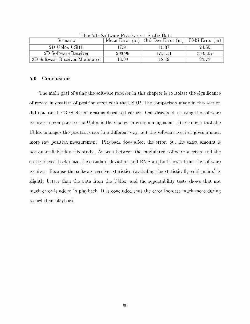
Table 5.1: Software Receiver vs. Static DataScenario Mean Error (m) Std Dev Error (m) RMS Error (m)

2D Ublox USRP 17.91 16.87 24.602D Software Receiver 208.96 1754.51 3533.67

2D Software Receiver Modulated 18.98 12.49 22.72

5.6 Conclusions

The main goal of using the software receiver in this chapter is to isolate the signi�cance

of record in creation of position error with the USRP. The comparison made in this section

did not use the GPSDO for reasons discussed earlier. One drawback of using the software

receiver to compare to the Ublox is the change in error management. It is known that the

Ublox manages the position error in a di�erent way, but the software receiver gives a much

more raw position measurement. Playback does a�ect the error, but the exact amount is

not quanti�able for this study. As seen between the modulated software receiver and the

static played back data, the standard deviation and RMS are both lower from the software

receiver. Because the software receiver statistics (excluding the statistically void points) is

slightly better than the data from the Ublox, and the repeatability tests shows that not

much error is added in playback. It is concluded that the error increase much more during

record than playback.

69

Chapter 6

Conclusions and Future Work

6.1 Observations and Conclusions

6.1.1 Limitations of USRP Evaluation

Limitations and shortcomings of the software and hardware are discussed in this section.

This section provides important segway into further work as a way to save time and improve

results. Some mistakes made during testing are discussed, while others limitations with the

USRP itself are discussed.

While gathering pseudorange data, there were multiple limitations. The �rst issue was

the software used for taking the data. The software Go-GPS requires Matlab and a constant

internet connection to work. Some errors occurred when compiling the data at the end which

was found late in post processing. When looking at these lower level measurements, certain

data points were dropped from individual satellites at di�erent points. Some were not seen

in the live data and others in the playback. This could not be explained from the research

done in this thesis.

With the dynamic testing, the �rst part of �normal� dynamic data was taken around

a standard street. The speed ranged from 25-55 mph but all of it was smooth driving with

gradual acceleration. The main signal errors were caused by degraded internet connectivity

which created spikes in the RTK position. There was a lot of drift from the high dynamic

data collected at the track. Both clock drift and position drift were observed. The only

problem with the CSAC data set, was the large amount of movement seen at the beginning

of the data set. This seems to be due to the second data set being recorded from a cold

start of the receiver. During all the tests with the Ublox, the starting method was taken

70

into account for post process reasons. It was noted if the receiver started from a cold start,

warm start, or hot start.

Because the software receiver is designed to work with a TCXO, it did not get a position

solution when using the GPSDO. Because of this, the data was recorded without the aid

of the GPSDO for timing. During the software receiver testing, a test is derived to see the

e�ects of recording and playing back with di�erent clock disciplines. When conducting this

test, if the clock was not the same during record and playback there would be no acquisition

of GPS signals.

6.1.2 Conclusions

The initial static result that compares the GPSDO and NON-GPSDO results shows the

need for accurate timing. Section 3.1.3 also shows the validity of record and playback for

static data when using more accurate timing. In Section 3.2 the CSAC was tested to see if

an even more accurate clock would give a more accurate position solution. The CSAC does

improve the position solution with a RMS error approximately 50 percent better than data

with a GPSDO. Because of this increase, it is concluded that the more accurate the clock

the better the record and playback results.

When testing for the validity of playing one data set back multiple times, the change

in position error is quite small. This validates the playback ability of the USRP and the

consistency of results. From the repeatability testing the results show errors between test

are approximately 1% of the overall error created by the USRP. In addition to playing the

signal back multiple times to one receiver, an attempt is made to play same data to di�erent

receivers. Each receiver reacts to the error created by the USRP in a similar way. Because

the statistics look proportionally correct the data recorded by the USRP can be tested across

receiver platforms.

The conclusions that were drawn form the result of the pseudorange testing were inter-

esting. The �rst noticeable result was the di�erence in availability of pseudoranges between

71

record and playback. The pseudorange measurements were not always captured at the same

time; some times there were measurements captured in the live data only and other times

the measurements were captured in the playback data only. This small piece of evidence

shows the amount of signal that is changed by recording and playing back the IF. The lack of

pseudoranges can be caused by any number of the following: dropped bit while recording to

the hard drive, o�set of the sample rate, spike in the noise and loss of signal, and degradation

through the USRP at certain times. These can be examined in the future in more detail.

Also during the pseudorange test a large change in doppler was seen. When looking at the

data it seems to mimic of an over damped system moving to steady state. This can account

for some of the issues when recording and playing back when an initial o�set is seen. Though

the changes are large in the beginning for longer data sets the USRP works adequately and

gives accurate position data.

The dynamic data shows a weakness of the USRP, the error increases signi�cantly when

used in a dynamic situation. The USRP can be used for dynamic situations but it is not as

accurate as static scenarios. The higher the dynamics, the larger the position error created

by the USRP. This can be seen graphically in Figure 4.15, which shows the higher speed

causing more error between the live and played back data. Because of this, it is suggested

that the USRP is used more for static and low velocity testing.

Finally, from the software receiver testing, it is concluded that both record and playback

add error to the position. The error from the clock is compounded in record and then

playback. It was determined that recording adds much more error than playback. Also it

was discovered during this test that the same clock has to be used for record and playback

or there will be no position solution.

72

6.2 Future Work

6.2.1 Measuring Di�erence Between Clocks

This thesis discovered the importance of timing for the USRP. Some e�ects of the clocks

were explored, but more correlation may be found with di�erent ways to collect data. Many

of the sources used for this thesis explored some clock drift over time, but they have not

been correlated to accuracy of GPS record and playback position. The error created by the

USRP clock needs to be correlated to position accuracy.

6.2.2 From IF to Pseudorange

In Section 3.4, conclusions are drawn about the error on the pseudoranges. The noise

creating the error is not introduced at the pseudorange level. Because of this, the error needs

to be traced back further to the source of the error at the IF level. A possible way to do this

could start by recording IF multiple ways and looking at the changes in error between them.

To do this a software receiver can be developed to see the errors from multiple IF recorders.

6.2.3 GPS Simulator

To more completely characterize the error on the USRP during record and playback of

GPS data, a simulator can be used. The simulator can output an RF signal that does not

have any errors on it. This can be used to see what errors the USRP adds by itself. The

simulator can also add speci�c types of errors, this method can pinpoint types of errors that

the USRP enhances. Using a simulator to pinpoint speci�c error modes will allow for better

use of the USRP in the future.

6.2.4 Mitigating Error

If the error created by the USRP can be predicted by an equation, the error can be

predicted and controlled in certain scenarios. With a completed model of the error created

73

by the USRP record an playback can be used to test speci�c qualities of GPS receivers.

Errors can be added and subtracted to simulate di�erent error.

74

Bibliography

[1] Microsemi Quantum SA.45s CSAC Chip-Scale Atomic Clock Data Sheet, 2014.

[2] A Annex. Global positioning system standard positioning service signal speci�cation,1995.

[3] Kai Borre, Dennis M Akos, Nicolaj Bertelsen, Peter Rinder, and Søren Holdt Jensen. Asoftware-de�ned GPS and Galileo receiver: a single-frequency approach. Springer, 2007.

[4] Alison Brown and Neil Gerein. Advanced gps hybrid simulator architecture. In Pro-ceedings of ION 57th Annual Meeting, volume 571. Albuquerque: New Mexico, 2001.

[5] Alison Brown, Neil Gerein, and Keith Taylor. Modeling and simulation of gps usingsoftware signal generation and digital signal reconstruction. In Proceedings of IONTechnical Meeting, 2000.

[6] Alison Brown and Bruce Johnson. Gps m-code and p-code signal simulation using anopen source radio platform. In Proceedings of the 24th International Technical Meetingof The Satellite Division of the Institute of Navigation (ION GNSS 2011), page 1494,2001.

[7] Alison Brown, Reece Tredway, and Robert Taylor. Gps signal simulation using opensource gps receiver platform. 2011.

[8] Ruihui Di, Senlin Peng, Steve Taylor, and Yu Morton. A usrp-based gnss and inter-ference signal generator and playback system. In Position Location and NavigationSymposium (PLANS), 2012 IEEE/ION, pages 470�478. IEEE, 2012.

[9] Carles Fernandez-Prades, Javier Arribas, Pau Closas, Carlos Aviles, and Luis Esteve.Gnss-sdr: an open source tool for researchers and developers. In Proceedings of the 24thInternational Technical Meeting of The Satellite Division of the Institute of Navigation(ION GNSS 2011), pages 780�0, 2001.

[10] Yanhong Kou, Yue Jiao, and YJ Morton. A unique software gps receiver and simulatorplatform for clock error measurement and simulation. In Proc. ION GNSS, pages 2923�2930, 2011.

[11] M Liso Nicolas, Ivan Artamonov, and T Kurner. Low-cost usrp sdr receiver for theinvestigation of multipath in�uence on gnss systems. In Antennas and Propagation(EuCAP), 2013 7th European Conference on, pages 2300�2304. IEEE, 2013.

75

[12] Robert Lutwak. The sa. 45s chip-scale atomic clock�early production statistics. PreciseTime and Time Interval, 2011.

[13] Lay Teen Ong. An usrp-based interference canceller. In Communication Systems(ICCS), 2012 IEEE International Conference on, pages 95�99. IEEE, 2012.

[14] Ozgur Ozdemir, Ridha Hamila, and Naofal Al-Dhahir. A usrp-based experimentaltestbed for ofdm systems impaired by i/q imbalance. In GCC Conference and Exhibition(GCC), 2013 7th IEEE, pages 98�102. IEEE, 2013.

[15] Christina Popper, Mario Strasser, and Srdjan Capkun. Anti-jamming broadcast com-munication using uncoordinated spread spectrum techniques. Selected Areas in Com-munications, IEEE Journal on, 28(5):703�715, 2010.

[16] James Rankin. Gps and di�erential gps: an error model for sensor simulation. InPosition Location and Navigation Symposium, pages 260�260. INSTITUTE OF ELEC-TRICAL & ELECTRONICS ENGINEERS INC, 1994.

[17] Ettus Research. Usrp n200/n210 networked series, September 2012.

[18] Eric Vinande Ruihui Di, Yu Morton. Performance analysis of a usrp based gps andglonass signal recording and playback system. 2013.

[19] Elizabeth A Thompson, Nathan Clem, Isaac Renninger, and Timothy Loos. Software-de�ned gps receiver on usrp-platform. Journal of Network and Computer Applications,35(4):1352�1360, 2012.

76