applied sciences

Article

Analysis of the Actual Power and EMF Exposure fromBase Stations in a Commercial 5G Network

Davide Colombi *, Paramananda Joshi, Bo Xu , Fatemeh Ghasemifard , Vignesh Narasarajuand Christer Törnevik

Ericsson Research, 164 83 Stockholm, Sweden; paramananda.joshi@ericsson.com (P.J.);bo.xu@ericsson.com (B.X.); fatemeh.ghasemifard@ericsson.com (F.G.); vignesh.narasaraju@ericsson.com (V.N.);christer.tornevik@ericsson.com (C.T.)* Correspondence: davide.colombi@ericsson.com; Tel.: +46-76-760-20-89

Received: 10 July 2020; Accepted: 29 July 2020; Published: 30 July 2020�����������������

Abstract: In this work, monitoring of the transmit power for several base stations operating in a live5G network (Telstra, Australia) was conducted with the purpose of analyzing the radio frequency(RF) electromagnetic field (EMF) exposure levels. The base stations made use of state-of-the-artmassive MIMO antennas utilizing beamforming in order to optimize the signal strength at the user’sdevice. In order to characterize the actual EMF exposure from 5G base stations, knowledge of theamount of power dynamically allocated to each beam is therefore of importance. Experimentaldata on the spatial distribution of the base stations’ transmit power were gathered directly fromthe network by extracting information on the radio and baseband operations. Out of more than13 million samples collected over 24 h, the maximum time-averaged power per beam direction wasfound to be well-below the theoretical maximum and lower than what was predicted by the existingstatistical models. The results show that assuming constant peak power transmission in a fixed beamdirection leads to an unrealistic EMF exposure assessment. This work provides insights relevant forthe standardization of EMF compliance assessment methodologies applicable for 5G base stations.

Keywords: mobile communication; EMF exposure; 5G; base stations; RF EMF compliance; massiveMIMO; antenna arrays; beamforming

1. Introduction

The first 5G NR (new radio) commercial networks were launched in 2019, and the number of5G subscriptions globally reached 13 million by the end of 2019 [1]. Like any other radio accesstechnology, 5G base stations (BSs) have to comply with radiofrequency (RF) electromagnetic field (EMF)exposure limits, such as those specified by the International Commission on Non-Ionizing RadiationProtection [2]. EMF measurement surveys of 5G BSs have been conducted in some countries [3,4],and typical exposure levels in areas accessible by the general public were found to be thousands oftimes below the limit values and similar to those of other existing mobile technologies (2G, 3G, and 4G).

5G makes use of beamforming and beam steering to adapt the antenna radiation pattern to thetime-varying traffic and the radio propagation conditions. This allows it to efficiently direct the energywhere needed, providing enhanced performance to the users. To be able to steer the beams over a rangeof angles, BS products make use of array antennas characterized by many elements, generally knownas massive MIMO antennas. Compared with conventional non-beamformed systems, massive MIMOBSs are characterized by a larger variability of transmitted signals in time and space. In order to takethis into account, specific measurement techniques to assess the exposure levels in proximity of 5Gmassive MIMO BSs have been developed [5–7].

Appl. Sci. 2020, 10, 5280; doi:10.3390/app10155280 www.mdpi.com/journal/applsci

Appl. Sci. 2020, 10, 5280 2 of 10

The effects of beamforming and traffic variation on the EMF exposure levels have been studiedby means of numerical simulations and statistical models [8,9]. Based on conservative assumptionson the data traffic and on the user distributions, these studies estimate the BS maximum power levelcontributing to EMF exposure in any beam direction. Since the beams are steered in order to provideservice to the connected users, the time-averaged power in each beam direction was found to bewell below the instantaneous peak (or theoretical maximum). According to [8], the 95th percentileof the transmitted power per beam would range between 7% and 22% of the theoretical maximum.These results have been verified by measurements conducted on massive MIMO BSs [10,11] of 4GLTE-Advanced networks. While a substantial amount of research available to date already shows thatmassive MIMO BSs do not constantly operate at the maximum power, experimental data specific for5G live networks are yet not available.

In this study, a large amount of experimental data of relevance for EMF exposure was collectedfrom a 5G NR commercial network. The dynamic of the spatial distribution of the transmit powerserving 5G users was continuously monitored for 25 massive MIMO BSs over 24 h. Data were extractedfrom network counters and events, which directly provide information on the BS baseband operations.In addition to the time-averaged transmit power, information on the beams scheduled by the BSs whenserving the connected users is obtained and processed. By this knowledge, the spatial distribution ofthe transmit power was determined. The method is developed in Section 2 and results on the actualpower are given in Section 3. A discussion, including implications of the results on EMF exposurefrom massive MIMO BSs is provided in Section 4 and some conclusions are drawn in Section 5.

This work is of interest to support the ongoing revision of IEC 62232 [5], which provides methodsto conduct EMF compliance assessment of massive MIMO BSs by taking the effects of beamforminginto consideration. The availability of 5G experimental data can be relevant to regulators when definingguiding principles on the usage of the actual maximum power to avoid unrealistic estimates of theEMF exposure levels.

2. Method

Measurement data were collected from 25 NR BSs of the Telstra commercial network in Australia.Telstra was among the first operators to launch 5G, and in January 2020, more than 100,000 5G-enabledmobile devices were connected to its network [12]. The massive MIMO BSs selected for this studywere located in dense urban areas, typically characterized by higher traffic than rural areas. The BSsoperated within the NR band 78 (3300–3800 MHz) with a channel bandwidth varying among the sitesand ranging from 40 to 80 MHz. The time division duplexing (TDD) downlink duty cycle, which isdefined as the fraction of the time available for downlink transmission to the total transmission time,was about 75%.

Ericsson Network Manager (ENM) was used to access information on the 5G BSs operation for24 h over a weekday at the end of January 2020. By means of gathering data directly through the ENM,it was possible to simultaneously collect information and statistics for many sites over a relativelylong period. Moreover, it allowed us to analyze the spatial distribution of the BS transmit powerin a three-dimensional space within the scan range of the antenna rather than having to conductmeasurements at a fixed location.

The transmit power per direction or more specifically the equivalent isotropic radiated power(EIRP) in azimuth and elevation (ϕ,θ) was determined as a function of time by continuously loggingtwo metrics:

• The total (cell-wide) time-averaged transmit power, Pavg;• The time-averaged gain, Gavg(ϕ,θ).

While the recently updated exposure guidelines, ICNIRP [2], have extended the averaging timeapplicable to whole-body exposure to thirty minutes, six minutes was applied in this study accordingto the previous version of the ICNIRP guidelines [13]. This choice was made in order to allow a direct

Appl. Sci. 2020, 10, 5280 3 of 10

comparison with what was predicted by the statistical models, e.g., [8], published when [2] was notyet available. Moreover, it might take some time until the updated ICNIRP guidelines are adopted innational regulations. Since the time-averaged power over thirty minutes is equal or less than what isobtained by averaging over six minutes, the results presented in this paper are also conservative withrespect to the latest ICNIRP guidelines.

2.1. Six-Minute Total (Cell-Wide) Time-Averaged Power (Pavg)

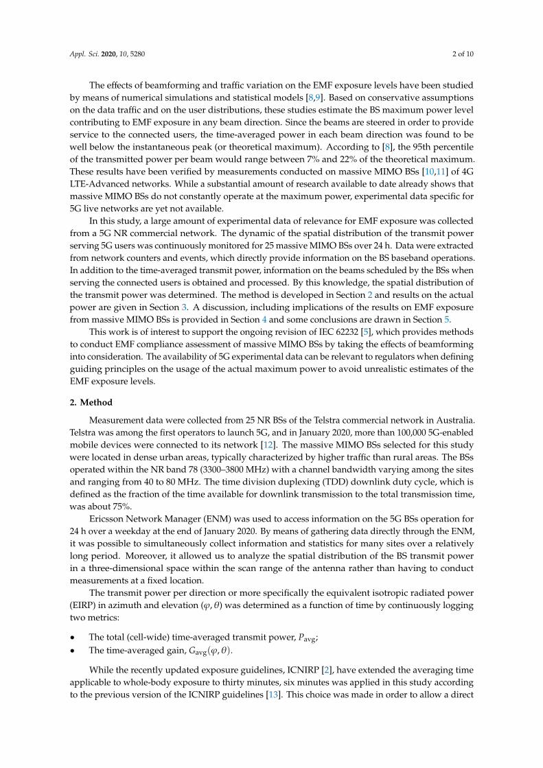
Pavg was assessed in the baseband based on the amount of physical resource blocks (PRBs)scheduled by the BS for downlink transmission. By summing up the power over all transmission timeintervals, a sample of the six-minute time-averaged transmit power was generated every 600 ms andthe distribution of the time-averaged power was then reported through the ENM every fifteen minutes(a typical reporting interval for network counters). The reported values of the time-averaged powerwere organized into bins characterized by a width of 2.5% with respect to the maximum available power(i.e., corresponding to 100% of the PRB usage). Therefore, a total of 1500 six-minute time-averagedtransmit power samples collected over 15 min were distributed over a total of 40 bins (ranging from0% to 100%). It is worth noticing that each sample was determined by applying a rolling average andthe reported distribution is therefore representative of any six-minute interval within fifteen minutes.Figure 1 provides an illustrative example of the data as collected through the network counter.

Appl. Sci. 2020, 10, x FOR PEER REVIEW 3 of 10

to the previous version of the ICNIRP guidelines [13]. This choice was made in order to allow a direct

comparison with what was predicted by the statistical models, e.g., [8], published when [2] was not

yet available. Moreover, it might take some time until the updated ICNIRP guidelines are adopted in

national regulations. Since the time-averaged power over thirty minutes is equal or less than what is

obtained by averaging over six minutes, the results presented in this paper are also conservative with

respect to the latest ICNIRP guidelines.

2.1. Six-Minute Total (Cell-Wide) Time-Averaged Power (𝑃𝑎𝑣𝑔)

𝑃avg was assessed in the baseband based on the amount of physical resource blocks (PRBs)

scheduled by the BS for downlink transmission. By summing up the power over all transmission time

intervals, a sample of the six-minute time-averaged transmit power was generated every 600 ms and

the distribution of the time-averaged power was then reported through the ENM every fifteen

minutes (a typical reporting interval for network counters). The reported values of the time-averaged

power were organized into bins characterized by a width of 2.5% with respect to the maximum

available power (i.e., corresponding to 100% of the PRB usage). Therefore, a total of 1500 six-minute

time-averaged transmit power samples collected over 15 min were distributed over a total of 40 bins

(ranging from 0% to 100%). It is worth noticing that each sample was determined by applying a

rolling average and the reported distribution is therefore representative of any six-minute interval

within fifteen minutes. Figure 1 provides an illustrative example of the data as collected through the

network counter.

Figure 1. Example of a six-minute time-averaged transmit power distribution (normalized) for a BS

over a fifteen-minute interval. Each bar shows the number of samples falling into a specific range of

values (100% would correspond to the BS operating at the maximum available power continuously

for 6 minutes). The overlaying text represents the raw data as collected from the ENM, i.e., indicating

that 966 samples of 𝑃avg belonged to the 0–2.5% interval, 30 to 2.5–5%, 32 to 5–7.5%...304 to 22.5–25%.

No samples in the example were obtained above the 22.5–25% interval.

2.2. Six-Minute Time-Averaged Gain (𝐺𝑎𝑣𝑔)

𝑃avg provides a measure of the total cell-wide time-averaged transmit power, but it does not

provide information on its spatial distribution, which for a massive MIMO BS will vary over time

depending on the beam selected for transmission. This was addressed by monitoring the BS antenna

radiation patterns during operation. While 3GPP allows for different beamforming schemes [14], the

software running on the selected BSs at the time of the investigation supported single-user MIMO

codebook-based beamforming with 8 CSI-RS ports. In this configuration, user equipment (UE) makes

use of channel state information (CSI) reference signals (RS) transmitted from the BS to measure the

radio channel quality. Based on this, the UE sends the CSI report, which contains a precoder matrix

indicator (PMI), a rank indicator (RI), and some other indicators, to the BS. Then, the BS selects the

corresponding beam(s) for downlink transmission of traffic data using the reported PMI and RI. The

Figure 1. Example of a six-minute time-averaged transmit power distribution (normalized) for a BSover a fifteen-minute interval. Each bar shows the number of samples falling into a specific range ofvalues (100% would correspond to the BS operating at the maximum available power continuouslyfor 6 minutes). The overlaying text represents the raw data as collected from the ENM, i.e., indicatingthat 966 samples of Pavg belonged to the 0–2.5% interval, 30 to 2.5–5%, 32 to 5–7.5%...304 to 22.5–25%.No samples in the example were obtained above the 22.5–25% interval.

2.2. Six-Minute Time-Averaged Gain (Gavg)

Pavg provides a measure of the total cell-wide time-averaged transmit power, but it does notprovide information on its spatial distribution, which for a massive MIMO BS will vary over timedepending on the beam selected for transmission. This was addressed by monitoring the BS antennaradiation patterns during operation. While 3GPP allows for different beamforming schemes [14],the software running on the selected BSs at the time of the investigation supported single-user MIMOcodebook-based beamforming with 8 CSI-RS ports. In this configuration, user equipment (UE) makesuse of channel state information (CSI) reference signals (RS) transmitted from the BS to measurethe radio channel quality. Based on this, the UE sends the CSI report, which contains a precodermatrix indicator (PMI), a rank indicator (RI), and some other indicators, to the BS. Then, the BS selectsthe corresponding beam(s) for downlink transmission of traffic data using the reported PMI and RI.The PMI and RI can be seen as a reference into a codebook of antenna precoding matrix (known

Appl. Sci. 2020, 10, 5280 4 of 10

by both the BS and the UE) corresponding to a certain beam shape. The dynamic of the antennaradiation patterns was therefore studied by logging PMI and RI reported periodically to the BS bythe UEs. As long as a UE is ‘active’ (i.e., receiving data from the BS), the BS will request PMI andRI reporting from it. Therefore, the time interval between consecutive reports collected in this studyvaried depending on the number of connected UEs with non-empty downlink transmit buffer (with amedian value of 70 ms). For this study, a total number of about 13 million PMI and RI samples werecollected in the 24 h.

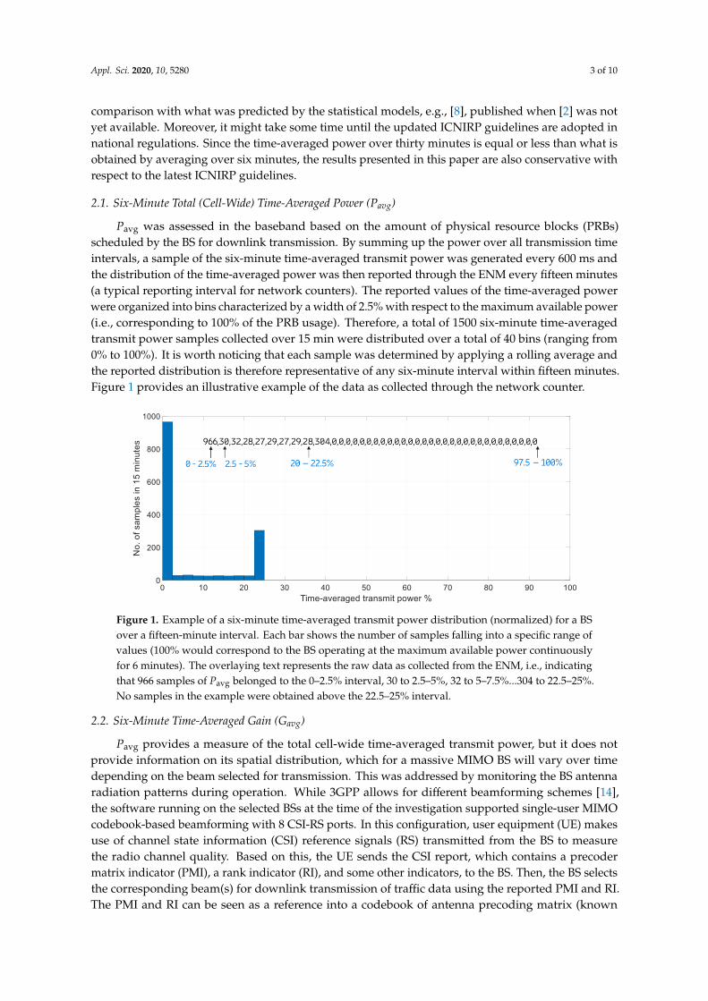
In Figure 2, antenna radiation patterns are shown as a function of the azimuth angle fora small subset of the available beam configurations (four out of sixteen patterns available for rank1 transmission are displayed; transmission up to rank 4 was supported by the BSs [14]). For the8 CSI-RS port codebook-based beamforming that was configured on the selected sites, only beamsteering in the azimuth plane was supported (no vertical beam steering). A discussion about theeffects of different beamforming implementations on the evaluation of the actual maximum exposureis provided in Section 4.

The time-averaged gain, Gavg (ϕ,θ), was obtained by averaging the antenna radiation patternscorresponding to all PMI and RI reported by all ‘active’ UEs to the BS within every six-minute interval(a moving average was applied) over the 24 h. Gavg was calculated at any time when a new CSI reportwas received. Those time intervals, for which no PMI and RI were reported, meaning that no datatraffic was served by the BS or that the data logging had failed, were excluded from the analysis.

Appl. Sci. 2020, 10, x FOR PEER REVIEW 4 of 10

PMI and RI can be seen as a reference into a codebook of antenna precoding matrix (known by both

the BS and the UE) corresponding to a certain beam shape. The dynamic of the antenna radiation

patterns was therefore studied by logging PMI and RI reported periodically to the BS by the UEs. As

long as a UE is ‘active’ (i.e., receiving data from the BS), the BS will request PMI and RI reporting

from it. Therefore, the time interval between consecutive reports collected in this study varied

depending on the number of connected UEs with non-empty downlink transmit buffer (with a

median value of 70 ms). For this study, a total number of about 13 million PMI and RI samples were

collected in the 24 h.

In Figure 2, antenna radiation patterns are shown as a function of the azimuth angle for a small

subset of the available beam configurations (four out of sixteen patterns available for rank 1

transmission are displayed; transmission up to rank 4 was supported by the BSs [14]). For the 8 CSI-

RS port codebook-based beamforming that was configured on the selected sites, only beam steering

in the azimuth plane was supported (no vertical beam steering). A discussion about the effects of

different beamforming implementations on the evaluation of the actual maximum exposure is

provided in Section 4.

The time-averaged gain, 𝐺avg (𝜑, 𝜃), was obtained by averaging the antenna radiation patterns

corresponding to all PMI and RI reported by all ‘active’ UEs to the BS within every six-minute interval

(a moving average was applied) over the 24 h. 𝐺avg was calculated at any time when a new CSI report

was received. Those time intervals, for which no PMI and RI were reported, meaning that no data

traffic was served by the BS or that the data logging had failed, were excluded from the analysis.

(a) (b)

Figure 2. (a) Antenna radiation patterns for four beam configurations (in different colors) in the

azimuth plane (𝜃 = 90°). The values in the polar plot are normalized to the peak gain of the broadside

beam and presented in a logarithmic scale in dB. Only a subset of the available BS beams is shown.

(b) Reference system with respect to the antenna.

2.3. Six-Minute Time-Averaged EIRP (𝐸𝐼𝑅𝑃𝑎𝑐𝑡)

By combining knowledge of the time-averaged transmit power, 𝑃avg, with the average gain,

𝐺avg(𝜑, 𝜃), the six-minute time-averaged actual EIRP was determined according to:

𝐸𝐼𝑅𝑃act(𝜑, 𝜃, 𝑡) = 𝐺avg (𝜑, 𝜃, 𝑡)× 𝑃avg (𝑡) (1)

𝐸𝐼𝑅𝑃act provides a measure of the spatial distribution of the time-averaged transmit power, and

it is therefore directly related to EMF exposure. Equation (1) implicitly assumes the time-averaged

power 𝑃avg to be equally distributed among the beam configurations reported within the same six-

minute interval. In addition, while 𝑃avg provides a measure of the total transmit power, including

the broadcast channel, 𝐺avg is determined based on the antenna pattern only used for data traffic.

Figure 2. (a) Antenna radiation patterns for four beam configurations (in different colors) in the azimuthplane (θ = 90◦). The values in the polar plot are normalized to the peak gain of the broadside beam andpresented in a logarithmic scale in dB. Only a subset of the available BS beams is shown. (b) Referencesystem with respect to the antenna.

2.3. Six-Minute Time-Averaged EIRP (EIRPact)

By combining knowledge of the time-averaged transmit power, Pavg, with the average gain,Gavg(ϕ,θ), the six-minute time-averaged actual EIRP was determined according to:

EIRPact(ϕ,θ, t) = Gavg (ϕ,θ, t ) × Pavg(t) (1)

EIRPact provides a measure of the spatial distribution of the time-averaged transmit power, and itis therefore directly related to EMF exposure. Equation (1) implicitly assumes the time-averaged powerPavg to be equally distributed among the beam configurations reported within the same six-minuteinterval. In addition, while Pavg provides a measure of the total transmit power, including the broadcastchannel, Gavg is determined based on the antenna pattern only used for data traffic. Since the antennagain for the broadcast signals is several dB lower than the peak antenna gain for the traffic beams,

Appl. Sci. 2020, 10, 5280 5 of 10

EIRPact provides a conservative estimate of the time-averaged EIRP. In any case, the broadcast signal in5G NR only counts for a very small amount of the BS maximum transmit power (the resource elementsallocated for transmission of the synchronization signal block are typically lower than 0.1% of the totalavailable [6]).

The value of Pavg at time t was approximated by the largest six-minute averaged power samplereported in the corresponding fifteen-minute interval as extracted from the network. With reference tothe fifteen-minute interval in Figure 1, the selected Pavg would be 23.75% (i.e., the center value of thelargest bin, for which at least one sample was observed). This is a conservative assumption, since formany instances of t within the fifteen minutes, the six-minute time-averaged transmit power could belower (e.g., in Figure 1 most of the samples belong to the bin corresponding to a power of 0 to 2.5%).As shown in Section 3, this assumption might lead to a large overestimate of EIRPact.

3. Results

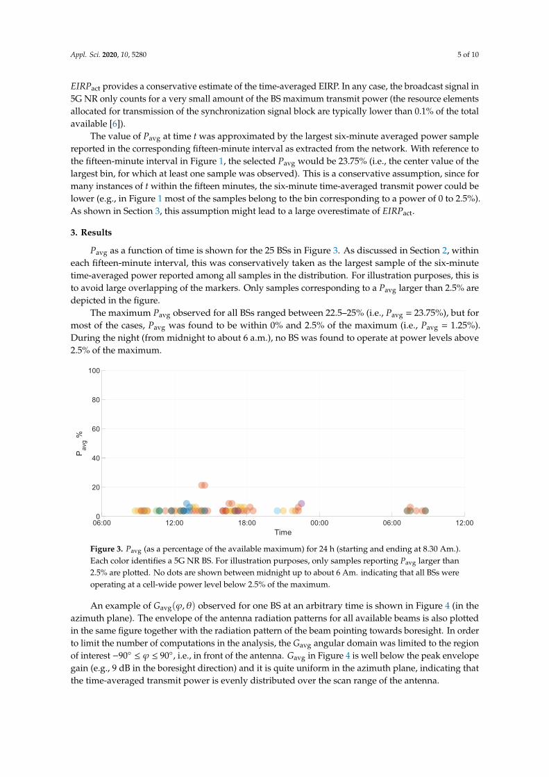
Pavg as a function of time is shown for the 25 BSs in Figure 3. As discussed in Section 2, withineach fifteen-minute interval, this was conservatively taken as the largest sample of the six-minutetime-averaged power reported among all samples in the distribution. For illustration purposes, this isto avoid large overlapping of the markers. Only samples corresponding to a Pavg larger than 2.5% aredepicted in the figure.

The maximum Pavg observed for all BSs ranged between 22.5–25% (i.e., Pavg = 23.75%), but formost of the cases, Pavg was found to be within 0% and 2.5% of the maximum (i.e., Pavg = 1.25%).During the night (from midnight to about 6 a.m.), no BS was found to operate at power levels above2.5% of the maximum.

Appl. Sci. 2020, 10, x FOR PEER REVIEW 5 of 10

Since the antenna gain for the broadcast signals is several dB lower than the peak antenna gain for

the traffic beams, 𝐸𝐼𝑅𝑃act provides a conservative estimate of the time-averaged EIRP. In any case,

the broadcast signal in 5G NR only counts for a very small amount of the BS maximum transmit

power (the resource elements allocated for transmission of the synchronization signal block are

typically lower than 0.1% of the total available [6]).

The value of 𝑃avg at time 𝑡 was approximated by the largest six-minute averaged power sample

reported in the corresponding fifteen-minute interval as extracted from the network. With reference

to the fifteen-minute interval in Figure 1, the selected 𝑃avg would be 23.75% (i.e., the center value of

the largest bin, for which at least one sample was observed). This is a conservative assumption, since

for many instances of 𝑡 within the fifteen minutes, the six-minute time-averaged transmit power

could be lower (e.g., in Figure 1 most of the samples belong to the bin corresponding to a power of 0

to 2.5%). As shown in Section 3, this assumption might lead to a large overestimate of 𝐸𝐼𝑅𝑃act.

3. Results

𝑃avg as a function of time is shown for the 25 BSs in Figure 3. As discussed in Section 2, within

each fifteen-minute interval, this was conservatively taken as the largest sample of the six-minute

time-averaged power reported among all samples in the distribution. For illustration purposes, this

is to avoid large overlapping of the markers. Only samples corresponding to a 𝑃avg larger than 2.5%

are depicted in the figure.

The maximum 𝑃avg observed for all BSs ranged between 22.5–25% (i.e., 𝑃avg = 23.75%), but for

most of the cases, 𝑃avg was found to be within 0% and 2.5% of the maximum (i.e., 𝑃avg = 1.25%).

During the night (from midnight to about 6 a.m.), no BS was found to operate at power levels above

2.5% of the maximum.

Figure 3. 𝑃avg (as a percentage of the available maximum) for 24 h (starting and ending at 8.30 Am.).

Each color identifies a 5G NR BS. For illustration purposes, only samples reporting 𝑃avg larger than

2.5% are plotted. No dots are shown between midnight up to about 6 Am. indicating that all BSs were

operating at a cell-wide power level below 2.5% of the maximum.

An example of 𝐺avg(𝜑, 𝜃) observed for one BS at an arbitrary time is shown in Figure 4 (in the

azimuth plane). The envelope of the antenna radiation patterns for all available beams is also plotted

in the same figure together with the radiation pattern of the beam pointing towards boresight. In

order to limit the number of computations in the analysis, the 𝐺avg angular domain was limited to

the region of interest −90° ≤ 𝜑 ≤ 90°, i.e., in front of the antenna. 𝐺avg in Figure 4 is well below the

peak envelope gain (e.g., 9 dB in the boresight direction) and it is quite uniform in the azimuth plane,

indicating that the time-averaged transmit power is evenly distributed over the scan range of the

antenna.

Figure 3. Pavg (as a percentage of the available maximum) for 24 h (starting and ending at 8.30 Am.).Each color identifies a 5G NR BS. For illustration purposes, only samples reporting Pavg larger than2.5% are plotted. No dots are shown between midnight up to about 6 Am. indicating that all BSs wereoperating at a cell-wide power level below 2.5% of the maximum.

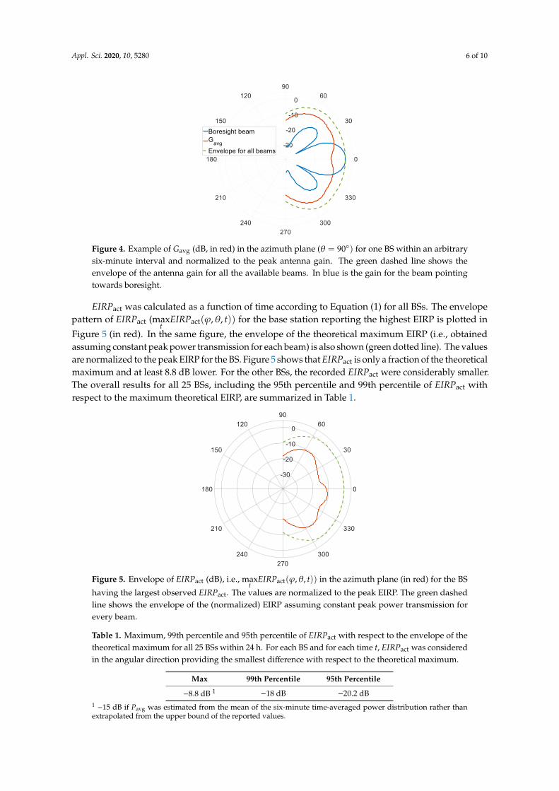
An example of Gavg(ϕ,θ) observed for one BS at an arbitrary time is shown in Figure 4 (in theazimuth plane). The envelope of the antenna radiation patterns for all available beams is also plottedin the same figure together with the radiation pattern of the beam pointing towards boresight. In orderto limit the number of computations in the analysis, the Gavg angular domain was limited to the regionof interest −90◦ ≤ ϕ ≤ 90◦, i.e., in front of the antenna. Gavg in Figure 4 is well below the peak envelopegain (e.g., 9 dB in the boresight direction) and it is quite uniform in the azimuth plane, indicating thatthe time-averaged transmit power is evenly distributed over the scan range of the antenna.

Appl. Sci. 2020, 10, 5280 6 of 10Appl. Sci. 2020, 10, x FOR PEER REVIEW 6 of 10

Figure 4. Example of 𝐺avg (dB, in red) in the azimuth plane (𝜃 = 90°) for one BS within an arbitrary

six-minute interval and normalized to the peak antenna gain. The green dashed line shows the

envelope of the antenna gain for all the available beams. In blue is the gain for the beam pointing

towards boresight.

𝐸𝐼𝑅𝑃act was calculated as a function of time according to Equation (1) for all BSs. The envelope

pattern of 𝐸𝐼𝑅𝑃act (max𝑡

𝐸𝐼𝑅𝑃act(𝜑, 𝜃, 𝑡)) for the base station reporting the highest EIRP is plotted in

Figure 5 (in red). In the same figure, the envelope of the theoretical maximum EIRP (i.e., obtained

assuming constant peak power transmission for each beam) is also shown (green dotted line). The

values are normalized to the peak EIRP for the BS. Figure 5 shows that 𝐸𝐼𝑅𝑃act is only a fraction of

the theoretical maximum and at least 8.8 dB lower. For the other BSs, the recorded 𝐸𝐼𝑅𝑃act were

considerably smaller. The overall results for all 25 BSs, including the 95th percentile and 99th

percentile of 𝐸𝐼𝑅𝑃act with respect to the maximum theoretical EIRP, are summarized in Table 1.

Figure 5. Envelope of 𝐸𝐼𝑅𝑃act (dB), i.e., max𝑡

𝐸𝐼𝑅𝑃act(𝜑, 𝜃, 𝑡)) in the azimuth plane (in red) for the BS

having the largest observed 𝐸𝐼𝑅𝑃act. The values are normalized to the peak EIRP. The green dashed

line shows the envelope of the (normalized) EIRP assuming constant peak power transmission for

every beam.

Table 1. Maximum, 99th percentile and 95th percentile of 𝐸𝐼𝑅𝑃act with respect to the envelope of the

theoretical maximum for all 25 BSs within 24 h. For each BS and for each time t, 𝐸𝐼𝑅𝑃act was

Figure 4. Example of Gavg (dB, in red) in the azimuth plane (θ = 90◦) for one BS within an arbitrarysix-minute interval and normalized to the peak antenna gain. The green dashed line shows theenvelope of the antenna gain for all the available beams. In blue is the gain for the beam pointingtowards boresight.

EIRPact was calculated as a function of time according to Equation (1) for all BSs. The envelopepattern of EIRPact (max

tEIRPact(ϕ,θ, t)) for the base station reporting the highest EIRP is plotted in

Figure 5 (in red). In the same figure, the envelope of the theoretical maximum EIRP (i.e., obtainedassuming constant peak power transmission for each beam) is also shown (green dotted line). The valuesare normalized to the peak EIRP for the BS. Figure 5 shows that EIRPact is only a fraction of the theoreticalmaximum and at least 8.8 dB lower. For the other BSs, the recorded EIRPact were considerably smaller.The overall results for all 25 BSs, including the 95th percentile and 99th percentile of EIRPact withrespect to the maximum theoretical EIRP, are summarized in Table 1.

Appl. Sci. 2020, 10, x FOR PEER REVIEW 6 of 10

Figure 4. Example of 𝐺avg (dB, in red) in the azimuth plane (𝜃 = 90°) for one BS within an arbitrary

six-minute interval and normalized to the peak antenna gain. The green dashed line shows the

envelope of the antenna gain for all the available beams. In blue is the gain for the beam pointing

towards boresight.

𝐸𝐼𝑅𝑃act was calculated as a function of time according to Equation (1) for all BSs. The envelope

pattern of 𝐸𝐼𝑅𝑃act (max𝑡

𝐸𝐼𝑅𝑃act(𝜑, 𝜃, 𝑡)) for the base station reporting the highest EIRP is plotted in

Figure 5 (in red). In the same figure, the envelope of the theoretical maximum EIRP (i.e., obtained

assuming constant peak power transmission for each beam) is also shown (green dotted line). The

values are normalized to the peak EIRP for the BS. Figure 5 shows that 𝐸𝐼𝑅𝑃act is only a fraction of

the theoretical maximum and at least 8.8 dB lower. For the other BSs, the recorded 𝐸𝐼𝑅𝑃act were

considerably smaller. The overall results for all 25 BSs, including the 95th percentile and 99th

percentile of 𝐸𝐼𝑅𝑃act with respect to the maximum theoretical EIRP, are summarized in Table 1.

Figure 5. Envelope of 𝐸𝐼𝑅𝑃act (dB), i.e., max𝑡

𝐸𝐼𝑅𝑃act(𝜑, 𝜃, 𝑡)) in the azimuth plane (in red) for the BS

having the largest observed 𝐸𝐼𝑅𝑃act. The values are normalized to the peak EIRP. The green dashed

line shows the envelope of the (normalized) EIRP assuming constant peak power transmission for

every beam.

Table 1. Maximum, 99th percentile and 95th percentile of 𝐸𝐼𝑅𝑃act with respect to the envelope of the

theoretical maximum for all 25 BSs within 24 h. For each BS and for each time t, 𝐸𝐼𝑅𝑃act was

Figure 5. Envelope of EIRPact (dB), i.e., maxt

EIRPact(ϕ,θ, t)) in the azimuth plane (in red) for the BS

having the largest observed EIRPact. The values are normalized to the peak EIRP. The green dashedline shows the envelope of the (normalized) EIRP assuming constant peak power transmission forevery beam.

Table 1. Maximum, 99th percentile and 95th percentile of EIRPact with respect to the envelope of thetheoretical maximum for all 25 BSs within 24 h. For each BS and for each time t, EIRPact was consideredin the angular direction providing the smallest difference with respect to the theoretical maximum.

Max 99th Percentile 95th Percentile

−8.8 dB 1 −18 dB −20.2 dB1−15 dB if Pavg was estimated from the mean of the six-minute time-averaged power distribution rather than

extrapolated from the upper bound of the reported values.

Appl. Sci. 2020, 10, 5280 7 of 10

The values in Figure 5 and Table 1 provide a conservative estimate of EIRPact. In fact, as describedin Section 2, Pavg used in Equation (1) was overestimated from the reported distribution of thesix-minute time-averaged power by selecting the sample with the highest transmit power in thefifteen-minute interval even though most of the six-minute time-averaged samples reported weremuch lower (see Figure 1). By using the mean of the distribution rather than the maximum value forPavg, the resulting EIRPact would be at least 15 dB (rather than 8.8 dB) below the theoretical maximum.

4. Discussion

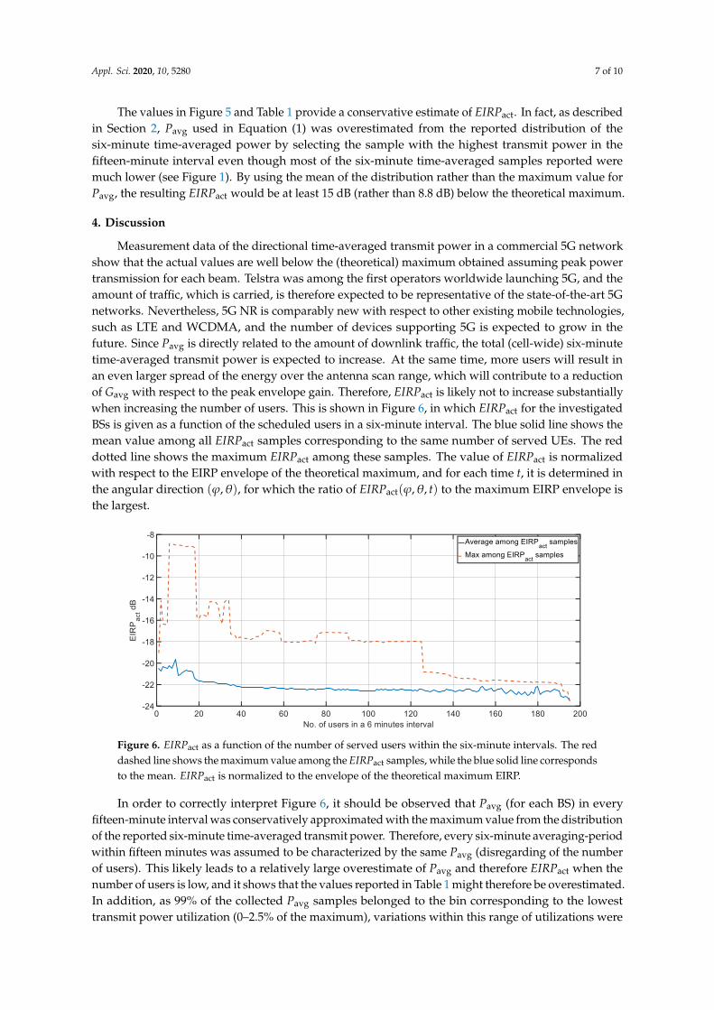
Measurement data of the directional time-averaged transmit power in a commercial 5G networkshow that the actual values are well below the (theoretical) maximum obtained assuming peak powertransmission for each beam. Telstra was among the first operators worldwide launching 5G, and theamount of traffic, which is carried, is therefore expected to be representative of the state-of-the-art 5Gnetworks. Nevertheless, 5G NR is comparably new with respect to other existing mobile technologies,such as LTE and WCDMA, and the number of devices supporting 5G is expected to grow in thefuture. Since Pavg is directly related to the amount of downlink traffic, the total (cell-wide) six-minutetime-averaged transmit power is expected to increase. At the same time, more users will result inan even larger spread of the energy over the antenna scan range, which will contribute to a reductionof Gavg with respect to the peak envelope gain. Therefore, EIRPact is likely not to increase substantiallywhen increasing the number of users. This is shown in Figure 6, in which EIRPact for the investigatedBSs is given as a function of the scheduled users in a six-minute interval. The blue solid line shows themean value among all EIRPact samples corresponding to the same number of served UEs. The reddotted line shows the maximum EIRPact among these samples. The value of EIRPact is normalizedwith respect to the EIRP envelope of the theoretical maximum, and for each time t, it is determined inthe angular direction (ϕ,θ), for which the ratio of EIRPact(ϕ,θ, t) to the maximum EIRP envelope isthe largest.

Appl. Sci. 2020, 10, x FOR PEER REVIEW 7 of 10

considered in the angular direction providing the smallest difference with respect to the theoretical

maximum.

Max 99th Percentile 95th Percentile

−8.8 dB 1 −18 dB −20.2 dB 1 −15 dB if 𝑃avg was estimated from the mean of the six-minute time-averaged power distribution

rather than extrapolated from the upper bound of the reported values.

The values in Figure 5 and Table 1 provide a conservative estimate of 𝐸𝐼𝑅𝑃act . In fact, as

described in Section 2, 𝑃avg used in Equation (1) was overestimated from the reported distribution

of the six-minute time-averaged power by selecting the sample with the highest transmit power in

the fifteen-minute interval even though most of the six-minute time-averaged samples reported were

much lower (see Figure 1). By using the mean of the distribution rather than the maximum value for

𝑃avg , the resulting 𝐸𝐼𝑅𝑃act would be at least 15 dB (rather than 8.8 dB) below the theoretical

maximum.

4. Discussion

Measurement data of the directional time-averaged transmit power in a commercial 5G network

show that the actual values are well below the (theoretical) maximum obtained assuming peak power

transmission for each beam. Telstra was among the first operators worldwide launching 5G, and the

amount of traffic, which is carried, is therefore expected to be representative of the state-of-the-art 5G

networks. Nevertheless, 5G NR is comparably new with respect to other existing mobile technologies,

such as LTE and WCDMA, and the number of devices supporting 5G is expected to grow in the

future. Since 𝑃avg is directly related to the amount of downlink traffic, the total (cell-wide) six-minute

time-averaged transmit power is expected to increase. At the same time, more users will result in an

even larger spread of the energy over the antenna scan range, which will contribute to a reduction of

𝐺avg with respect to the peak envelope gain. Therefore, 𝐸𝐼𝑅𝑃act is likely not to increase substantially

when increasing the number of users. This is shown in Figure 6, in which 𝐸𝐼𝑅𝑃act for the investigated

BSs is given as a function of the scheduled users in a six-minute interval. The blue solid line shows

the mean value among all 𝐸𝐼𝑅𝑃act samples corresponding to the same number of served UEs. The

red dotted line shows the maximum 𝐸𝐼𝑅𝑃act among these samples. The value of 𝐸𝐼𝑅𝑃act is

normalized with respect to the EIRP envelope of the theoretical maximum, and for each time t, it is

determined in the angular direction (𝜑, 𝜃), for which the ratio of 𝐸𝐼𝑅𝑃act(𝜑, 𝜃, 𝑡) to the maximum

EIRP envelope is the largest.

Figure 6. 𝐸𝐼𝑅𝑃act as a function of the number of served users within the six-minute intervals. The red

dashed line shows the maximum value among the 𝐸𝐼𝑅𝑃act samples, while the blue solid line

corresponds to the mean. 𝐸𝐼𝑅𝑃act is normalized to the envelope of the theoretical maximum EIRP.

Figure 6. EIRPact as a function of the number of served users within the six-minute intervals. The reddashed line shows the maximum value among the EIRPact samples, while the blue solid line correspondsto the mean. EIRPact is normalized to the envelope of the theoretical maximum EIRP.

In order to correctly interpret Figure 6, it should be observed that Pavg (for each BS) in everyfifteen-minute interval was conservatively approximated with the maximum value from the distributionof the reported six-minute time-averaged transmit power. Therefore, every six-minute averaging-periodwithin fifteen minutes was assumed to be characterized by the same Pavg (disregarding of the numberof users). This likely leads to a relatively large overestimate of Pavg and therefore EIRPact when thenumber of users is low, and it shows that the values reported in Table 1 might therefore be overestimated.In addition, as 99% of the collected Pavg samples belonged to the bin corresponding to the lowesttransmit power utilization (0–2.5% of the maximum), variations within this range of utilizations were

Appl. Sci. 2020, 10, 5280 8 of 10

not detected. As a result, while Pavg as used in Equation (1) is substantially constant, the spatial spreadof energy (represented by Gavg) will increase with increasing the number of users leading to a reductionof EIRPact.

5G NR massive MIMO BSs can also support a larger number of beams compared with the 8 CSI-RSports codebook-based beamforming software, which was running on the investigated sites (e.g., basedon 16 CSI-RS or 32 CSI-RS [14]). In addition to narrower beams, such configurations might also supportsteering of energy in elevation and not just within the azimuth plane. Moreover, if reciprocity-basedbeamforming (i.e., non-codebook) is supported, sounding reference signals transmitted by the UEs willbe used by the BS to estimate the radio channel, allowing energy to be transmitted in several differentpaths rather than in specific directions. By means of reciprocity-based beamforming, BSs mightalso simultaneously send different layers in separate beams to different users using the same timeand frequency resource (multi-user MIMO). For such solutions, an even larger spread of the BStransmit power over different propagation paths is to be expected. The experimental data obtainedfor 8 CSI-RS ports codebook-based beamforming are therefore expected to provide a conservativeestimate of the actual transmit power of relevance for EMF assessments compared with other (existingor upcoming) implementations.

Although the spreading of energy is deemed to increase when traffic increases, the results inSection 3 show that EIRPact is also well below the theoretical maximum for a limited number of activeusers. Out of about 13 million samples, including instances for which only one user was active withina six-minute interval, not a single case was found when any of the BSs would constantly schedulethe same beam with the maximum power. Mobile networks are in fact deployed to provide servicesto a myriad of UEs, with enough margins to address occasional traffic peaks without reaching trafficcongestion. When only a few users are served, the amount of traffic, and therefore the BS time-averagedtransmit power, will account for a small fraction of the available maximum. Moreover, even the sameUE might be served by different beams over time as a consequence of the changes in the propagationconditions or due to simultaneous transmission of parallel data streams (when two or more layers aretransmitted to the same UE, the allocated power will be simultaneously spread among different beams).

Network measurements provide an efficient tool to gather comprehensive information on theactual EMF levels of live network for several BSs and long periods. This is even more relevant for BSimplementing beamforming, as the gathering of data directly from the network manager allows one tostudy the distribution of the transmitted signal in the spatial domain rather than at a fixed location.At the same time, measurements conducted in-situ are complementary and equally important, as theyprovide a direct measure of the typical EMF exposure levels in areas accessible by the general public.Although results from in-situ measurement campaigns addressing EMF exposure for massive MIMOare already available (e.g., [10,11]), including 5G (e.g., [3,4,6]), additional data are desirable while 5Gservices become widely spread.

The maximum EIRPact reported in Section 3, obtained from an overestimate of Pavg was found tobe 8.8 dB below the theoretical maximum. This value would drop to −15 dB if Pavg was estimated fromthe mean of the six-minute time-averaged transmit power distribution reported for every fifteen-minuteinterval. EIRPact was determined with respect to the peak instantaneous EIRP including the effect ofthe TDD downlink duty cycle (TDC). This allows for a direct comparison with other studies availablein the literature for which the TDC factor was also included when evaluating the actual power ofmassive MIMO BSs.

The experimental values of EIRPact observed in this work are below the maximum actual powerlevels previously estimated by statistical and numerical models (e.g., [8,9]). According to a technicalreport from the International Electrotechnical Commission [15], the actual maximum transmit powerpredicted for a massive MIMO site with horizontal beam scanning would only correspond to about 25%(−6 dB) of the theoretical maximum (including the effect of 75% TDD downlink duty cycle). Such valuesare consistent with measurements previously conducted on massive MIMO BSs of commercial 4Gnetworks [10,11]. In [10], the actual maximum exposure was found to be about 8.5 dB lower than

Appl. Sci. 2020, 10, 5280 9 of 10

the theoretical maximum by using network counters like those utilized in this paper. In [11], fieldmeasurements conducted in front of a massive MIMO LTE antenna, led to exposure values (whenscaled for the maximum BS utilization) ranging from 10 dB to 7 dB below the theoretical maximum.

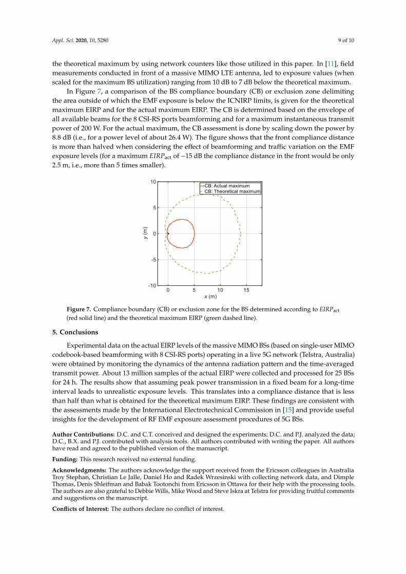
In Figure 7, a comparison of the BS compliance boundary (CB) or exclusion zone delimitingthe area outside of which the EMF exposure is below the ICNIRP limits, is given for the theoreticalmaximum EIRP and for the actual maximum EIRP. The CB is determined based on the envelope ofall available beams for the 8 CSI-RS ports beamforming and for a maximum instantaneous transmitpower of 200 W. For the actual maximum, the CB assessment is done by scaling down the power by8.8 dB (i.e., for a power level of about 26.4 W). The figure shows that the front compliance distanceis more than halved when considering the effect of beamforming and traffic variation on the EMFexposure levels (for a maximum EIRPact of −15 dB the compliance distance in the front would be only2.5 m, i.e., more than 5 times smaller).

Appl. Sci. 2020, 10, x FOR PEER REVIEW 9 of 10

The experimental values of 𝐸𝐼𝑅𝑃act observed in this work are below the maximum actual power

levels previously estimated by statistical and numerical models (e.g., [8,9]). According to a technical

report from the International Electrotechnical Commission [15], the actual maximum transmit power

predicted for a massive MIMO site with horizontal beam scanning would only correspond to about

25% (−6 dB) of the theoretical maximum (including the effect of 75% TDD downlink duty cycle). Such

values are consistent with measurements previously conducted on massive MIMO BSs of commercial

4G networks [10,11]. In [10], the actual maximum exposure was found to be about 8.5 dB lower than

the theoretical maximum by using network counters like those utilized in this paper. In [11], field

measurements conducted in front of a massive MIMO LTE antenna, led to exposure values (when

scaled for the maximum BS utilization) ranging from 10 dB to 7 dB below the theoretical maximum.

In Figure 7, a comparison of the BS compliance boundary (CB) or exclusion zone delimiting the

area outside of which the EMF exposure is below the ICNIRP limits, is given for the theoretical

maximum EIRP and for the actual maximum EIRP. The CB is determined based on the envelope of

all available beams for the 8 CSI-RS ports beamforming and for a maximum instantaneous transmit

power of 200 W. For the actual maximum, the CB assessment is done by scaling down the power by

8.8 dB (i.e., for a power level of about 26.4 W). The figure shows that the front compliance distance is

more than halved when considering the effect of beamforming and traffic variation on the EMF

exposure levels (for a maximum 𝐸𝐼𝑅𝑃act of −15 dB the compliance distance in the front would be

only 2.5 m, i.e., more than 5 times smaller).

Figure 7. Compliance boundary (CB) or exclusion zone for the BS determined according to 𝐸𝐼𝑅𝑃act

(red solid line) and the theoretical maximum EIRP (green dashed line).

5. Conclusions

Experimental data on the actual EIRP levels of the massive MIMO BSs (based on single-user

MIMO codebook-based beamforming with 8 CSI-RS ports) operating in a live 5G network (Telstra,

Australia) were obtained by monitoring the dynamics of the antenna radiation pattern and the time-

averaged transmit power. About 13 million samples of the actual EIRP were collected and processed

for 25 BSs for 24 h. The results show that assuming peak power transmission in a fixed beam for a

long-time interval leads to unrealistic exposure levels. This translates into a compliance distance that

is less than half than what is obtained for the theoretical maximum EIRP. These findings are

consistent with the assessments made by the International Electrotechnical Commission in [15] and

provide useful insights for the development of RF EMF exposure assessment procedures of 5G BSs.

Author Contributions: D.C. and C.T. conceived and designed the experiments; D.C. and P.J. analyzed the data;

D.C., B.X. and P.J. contributed with analysis tools. All authors contributed with writing the paper. All authors

have read and agreed to the published version of the manuscript.

Funding: This research received no external funding.

Figure 7. Compliance boundary (CB) or exclusion zone for the BS determined according to EIRPact

(red solid line) and the theoretical maximum EIRP (green dashed line).

5. Conclusions

Experimental data on the actual EIRP levels of the massive MIMO BSs (based on single-user MIMOcodebook-based beamforming with 8 CSI-RS ports) operating in a live 5G network (Telstra, Australia)were obtained by monitoring the dynamics of the antenna radiation pattern and the time-averagedtransmit power. About 13 million samples of the actual EIRP were collected and processed for 25 BSsfor 24 h. The results show that assuming peak power transmission in a fixed beam for a long-timeinterval leads to unrealistic exposure levels. This translates into a compliance distance that is lessthan half than what is obtained for the theoretical maximum EIRP. These findings are consistent withthe assessments made by the International Electrotechnical Commission in [15] and provide usefulinsights for the development of RF EMF exposure assessment procedures of 5G BSs.

Author Contributions: D.C. and C.T. conceived and designed the experiments; D.C. and P.J. analyzed the data;D.C., B.X. and P.J. contributed with analysis tools. All authors contributed with writing the paper. All authorshave read and agreed to the published version of the manuscript.

Funding: This research received no external funding.

Acknowledgments: The authors acknowledge the support received from the Ericsson colleagues in AustraliaTroy Stephan, Christian Le Jalle, Daniel Ho and Radek Wrzesinski with collecting network data, and DimpleThomas, Denis Shleifman and Babak Tootonchi from Ericsson in Ottawa for their help with the processing tools.The authors are also grateful to Debbie Wills, Mike Wood and Steve Iskra at Telstra for providing fruitful commentsand suggestions on the manuscript.

Conflicts of Interest: The authors declare no conflict of interest.

Appl. Sci. 2020, 10, 5280 10 of 10

References

1. Ericsson Mobility Report. Available online: https://www.ericsson.com/4acd7e/assets/local/mobility-report/documents/2019/emr-november-2019.pdf (accessed on 11 May 2020).

2. ICNIRP. Guidelines for limiting exposure to electromagnetic fields (100 kHz to 300 GHz). Health Phys. 2020.[CrossRef]

3. Ofcom. Electromagnetic Field (EMF) Measurements near 5G Mobile Phone Base Stations. Available online: https://www.ofcom.org.uk/__data/assets/pdf_file/0015/190005/emf-test-summary.pdf (accessed on 11 May 2020).

4. Telstra. 5 Surveys of 5G. Available online: http://1u0b5867gsn1ez16a1p2vcj1-wpengine.netdna-ssl.com/wp-content/uploads/2019/07/5-Surveys-of-5G-flyer-A4.pdf (accessed on 11 May 2020).

5. IEC TC106. IEC 62232: Determination of RF Field Strength, Power Density and SAR in the Vicinity ofRadiocommunication Base Stations for the Purpose of Evaluating Human Exposure (Committee Draft); IEC:Geneva, Switzerland, 2020.

6. Aerts, S.; Verloock, L.; Van Den Bossche, M.; Colombi, D.; Martens, L.; Törnevik, C.; Joseph, W. In-situmeasurement methodology for the assessment of 5G NR massive MIMO base station exposure at sub-6 GHzfrequencies. IEEE Access 2020, 7, 184658–184667. [CrossRef]

7. Keller, H. On the assessment of human exposure to electromagnetic fields transmitted by 5G NR base stations.Health Phys. 2019, 117, 541–545. [CrossRef] [PubMed]

8. Thors, B.; Furuskär, A.; Colombi, D.; Törnevik, C. Time-averaged realistic maximum power levels for theassessment of radio frequency exposure for 5G radio base stations using massive MIMO. IEEE Access 2017, 5,19711–19719. [CrossRef]

9. Baracca, P.; Weber, A.; Wild, T.; Grangeat, C. A statistical approach for RF exposure compliance boundaryassessment in massive MIMO systems. In Proceedings of the 22nd International ITG Workshop SmartAntennas (WSA), Bochum, Germany, 14–16 March 2018; pp. 1–6.

10. Colombi, D.; Joshi, P.; Pereira, R.; Thomas, D.; Shleifman, D.; Tootoonchi, B.; Xu, B.; Törnevik, C. Assessmentof actual maximum RF EMF exposure from radio base stations with massive MIMO antennas. In Proceedingsof the 2019 Photonics & Electromagnetics Research Symposium-Spring (PIERS-Spring), Rome, Italy,17–20 June 2019. [CrossRef]

11. Werner, R.; Knipe, P.; Iskra, S. A comparison between measured and computed assessments of the RFexposure compliance boundary of an in-situ radio base station massive MIMO antenna. IEEE Access 2019, 7,170682–170689. [CrossRef]

12. Telstra. What You Need to Know about Our 2020 Half-Year Financial Results. Available online: https://exchange.telstra.com.au/what-you-need-to-know-about-our-2020-half-year-financial-results/ (accessed on13 May 2020).

13. ICNIRP. Guidelines for limiting exposure to time-varying electric magnetic and electromagnetic fields (up300 GHz). Health Phys. 1998, 74, 494–522.

14. 3GPP. 5G; NR; Physical Layer Procedures for Data (3GPP TS 38.214 version 15.9.0 Release 15). Available online:https://www.etsi.org/deliver/etsi_ts/138200_138299/138214/15.09.00_60/ts_138214v150900p.pdf (accessed on14 May 2020).

15. IEC TC106. IEC 62669 Ed.2: Case Studies Supporting IEC 62232—Determination of RF Field Strength, PowerDensity and SAR in the Vicinity of Radiocommunication Base Stations for the Purpose of Evaluating Human Exposure;IEC: Geneva, Switzerland, 2020.

© 2020 by the authors. Licensee MDPI, Basel, Switzerland. This article is an open accessarticle distributed under the terms and conditions of the Creative Commons Attribution(CC BY) license (http://creativecommons.org/licenses/by/4.0/).